Q-Theory and Real Business Cycle Analytics 1

Miles S. KIMBALLUniversity of Michigan

September 2, 2003

1I would like to thank Philippe Weil, Matthew Shapiro and Kenneth West fortheir encouragement in writing this paper and many cohorts of students who gavereactions to the initial, rough versions of this material.

Abstract

A mathematical and graphical treatment of the Q-theory extension of theBasic Real Business Cycle model of Prescott indicates that several key re-sults are robust to both investment adjustment costs and to variation in theshape of the utility function and the production function while other custom-ary results are fragile. It also demonstrates some of the richness of generalequilibrium analysis. One key result relevant to recent debates about the em-pirical effects of technology is that an immediate, permanent improvementin technology unavoidably raises output, investment and the real interestrate, given uncontroversial assumptions such as normality of consumptionand leisure and constant returns to scale in production. A permanent in-crease in government purchases financed by an increase in lump-sum taxes isalso shown to unambiguously raise output, investment and the real interestrate.

1 Introduction

Since the eclipse of the purely literary approach to economics, the three pri-mary modes of economic analysis have been mathematical analysis, computersimulation, and statistical analysis of empirical data. Research projects tendto combine these three modes in varying shares. Because Real Business CycleTheory arose at a time of cheap computing power, computer simulation hasbeen the dominant mode of analysis in studying Real Business Cycle models.Theory in the sense of a thorough mathematical analysis has remained rela-tively underdeveloped compared to the rich development of a computationalunderstanding of themes and variations on Real Business Cycle models. Adiminishing marginal productivity argument suggests the value of further de-velopment of the mathematical analysis of Real Business Cycle models. Thispaper explores what can be gained from pushing further the mathematicalanalysis of stripped-down Real Business Cycle models by a thorough appli-cation of standard tools in the economist’s toolkit: control theory, duality,and the even more basic tool of graphical analysis.

One strength of a theoretical analysis is that it allows one to look atgeneral functional forms and a wide range of parameter values to distinguishwhich results are general and which ones are special to particular functionalforms.1 The approach in this paper will be to start with very general func-tional forms and then narrow the focus with assumptions on the key functionsthat have a transparent economic meaning.

Substantively, this paper analyzes the Basic Real Business Cycle Modelfamiliar from Prescott (1986) and the extension of this model that incor-porates Hayashi’s (1982) Neoclassical interpretation of Tobin’s Q-theory.Equivalently, it analyzes the extension of Abel and Blanchard’s () generalequilibrium Q-theory model that allows for variable labor supply. The styleof analysis is inspired by papers such as Cass (), Abel and Blanchard ()and Mankiw ()—a style emphasizing graphical analysis centered around thephase diagram.2

1For example, motivated by the arguments in Basu and Kimball (2002) and the empiri-cal evidence cited there that consumption and labor are unlikely to be additively separablein the utility function, one of the key dimensions of generality I allow for in this paper isnonseparability between consumption and labor.

2Because this style of analysis has pedagogical as well as substantive value, this paper iswritten with several audiences in mind, not least of which is the audience of graduate stu-

1

Although in relative terms, the amount of theory on Real Business Cyclemodels pales in comparison to the amount of computational work, in absoluteterms, there is a large quantity of theoretical papers on Real Business Cyclemodels. Some of the more obvious examples are Barro and King (),King,Plosser and Rebelo (1988), Rogerson (), Benhabib, Rogerson and Wright(1991), and Campbell (1994). But each of these papers and others in theliterature has other objectives and does not have this focus on the graphicalanalysis of the Prescott’s (1986) Basic Real Business Cycle Models or it Q-theory extension. In general, two factors that may have excessively inhibitedthe literature from pursuing such a graphical treatment are (1) a preferencefor formulating business models in discrete time, which makes phase diagramsless natural and (2) a belief that uncertainty makes the use of perfect foresightmodels inappropriate. It is worth dealing with each of these concerns upfront.

The modest language barrier between discrete and continuous time is un-fortunate, since with few exceptions continuous and discrete-time models getat the very same economics. As a formal matter, continuous time is particu-larly convenient when working with phase diagrams and often simplifies for-mulas, while side-stepping having to specify inconsequential details of timing;discrete time is easier to work with computationally and when using recursivetechniques in proofs. But as long as the length of the period in discrete timemodels is allowed to vary parametrically, discrete-time models are essentiallyequivalent in their economics to the corresponding continuous-time models.3

For example, computational power is now sufficient that it is a trivial mat-ter to implement discrete-time business cycle models with time periods of

dents in economics. I hope that more experienced economists will forgive my explanationsof certain things that may seem obvious.

3When the length of a period is routinely fixed at one quarter or one year, ratherthan being varied parametrically, certain dangers and temptations arise. For one thing,there are issues like those discussed in Hall (1988) with handling time-averaged data thatwould be easy to miss when thinking in terms of just one time unit. The issues with timeaveraging illustrate why the fact that data often comes with a quarterly frequency is nota sufficient reason for fixing a model’s time interval unalterably at one quarter. Second,when the period is routinely fixed at a quarter, it is easy to fall into the implicit and oftenundefended calibration of key parameters by the arbitrary length of the period. It is noaccident that models often assume that prices are fixed for three months, that the velocityof money is four times per year, or in an oligopolistic supergame that the length of timea firm can get away with undercutting its rivals is three months.

2

one hundredth of a year or less to make the gap between discrete-time andcontinuous-time models negligible. Even a quarter is a short enough lengthof time that the difference between one quarter and Thus, the continuous-time and discrete-time versions of a business cycle model, each convenientfor certain purposes, should both be part of the dialogue about that model.

As for uncertainty, it is true that uncertainty can cause departures fromcertainty equivalence, but in representative agent macro models, these depar-tures are typically small. This is for the simple reason that macroeconomicannual standard deviations are typically on the order of, say, 3% or .03, whichimplies a variance of only about .0009 per year to interact with any relevantcurvature of the functional forms. The products of small variances with mod-est curvatures are often reasonable to neglect, as is done routinely when doinglog-linear computations such as those implemented by the AIM program. Ifone is making a certainty-equivalence approximation for computational pur-poses, a log-linearized perfect foresight model will deliver exactly the sameimpulse responses. In other words, in representative agent macro models,the certainty equivalence approximation is typically good enough that un-certainty, while a major force ex post, is only a minor force ex ante. In theearly days of phase diagram analysis, some authors were a bit embarrassedat the seeming need to discuss the effects of shocks that were completelyunforeseen, but the justification for the analytical procedure in question ismuch stronger. It is simply the use of the certainty-equivalence approxima-tion ex ante with the ex post analysis of the effects of the realization of ashock that had the potential to go in either direction. In principal, the im-pulse responses deduced from a perfect foresight model could be combinedwith variances and covariance of shocks to get the variances and covariancesof macroeconomic variables that Prescott (1986) recommends focusing on tosee how well a model is doing, but in recent years, macroeconomists havegradually been coming around to the view that the simulated impulse re-sponses themselves are often more transparently informative of a model’sworkings than variance-covariance matrices.

After all such programmatic statements, the proof of the pudding is stillin the eating. To advertise the menu of what follows from studying the BasicRBC model and the QRBC model, here are some of the most interestingresults established and discussed in what follows.

• In both the Basic RBC Model and in the QRBC model, regardless of

3

functional forms, if the utility function has normal consumption andleisure, an immediate, permanent improvement in technology cannotcause output or investment to fall on impact. Moreover, a phased-inimprovement in technology can only cause output or investment to fallif consumption rises.

• In both models, a positive permanent technology shock or separablegovernment purchases shock raises investment and Q, and unambigu-ously raises the real interest rate on impact. Thus, in general equilib-rium, interest rate effects on investment are necessarily overwhelmedby changes in the demand for capital services reflected by the rentalrate of capital in reaction to permanent technology and fiscal shocks.

• Regardless of the complexity of the driving shock processes, the be-havior of the model economy at any point in time can be reduced to afew dimensions: the capital stock is a sufficient statistic for the past,the marginal value of capital is a sufficient statistic for the future, andthese plus the current values of the exogenous variables are enough todetermine the current values of all of the endogenous variables.

Following the advice of Polya (1957) for tackling math problems, the firstfew sections do a fair bit of pre-processing of the elements of the model,so that the hard core of the problem of characterizing the QRBC model isrevealed.

One element of pre-processing that should be done before doing anythingelse is detrending. In terms of understanding the real world, it makes senseto think in terms of a model with steady-state growth. For this application,think of the steady-state growth as coming from exogenous trend growth intechnology and population. The model can then be detrended by dividingquantities through by their trend values and adjusting interest rates, rentalrates, utility discount rates and depreciation rates (or the equivalent) appro-priately. This transformation is standard, so I do not do it explicitly. Think-ing of an ostensibly static model as a detrended version of a model withexogenously-driven trend growth does affect the appropriate calibration ofthe model because of the adjustments to rates just mentioned, but does notaffect the analysis itself—the tools for analyzing a static model are perfectlygood for analyzing the departures from trend of a model with exogenously-

4

driven trend growth.4 The consistency of labor augmenting technologicalprogress with trend growth motivates the interest in labor-augmenting tech-nology shocks below. (Technology has an upward trend, but may improvein fits and starts.) In the absence of trend improvement in the home pro-duction technology at exactly the same rate as the market technology, onecan also argue that consistency with a model that has steady-state growthshould also impose an extra constraint on the utility function, a la King,Plosser and Rebelo (), but since this constraint on the utility function willbe discussed as an optional extra assumption since it is not central to theanalysis.

2 The Social Planner’s Problem

The QRBC Model is the solution to the following social planner’s problem:

V (K0) = maxC,N

∫ ∞

0e−ρtU(C,N) dt (1)

subject to

K = KJ

(F (K,N, Z)− C −G

K

)(2)

and

K(0) = K0.

Time zero is the moment when information about the realization of ashock arrives. K is the capital stock. V (K0) is the optimized value giveninitial capital stock K0. C and N are the consumption and the labor hoursof the infinitely-lived representative consumer, ρ is the impatience parameter(the utility discount rate), K is the capital stock, Z is the level of labor-augmenting technology and G is exogenously given government purchasesthat may add to utility in an additively separable way that is not explic-itly represented, but does not have any direct interaction with U(C,N) orF (K, N). Many other exogenous government policy, technology and prefer-ence shifters could be considered after appropriate modifications of the model

4Of course, to analyze the effects of changes in the trend growth rate of technology orpopulation, it would be better to use a model that represents growth explicitly.

5

(including shocks to home production technology that are observationallyequivalent to preference shifters), but it is enough here to concentrate onlabor-augmenting technology and government purchases that have benefitsthat are additively separable from what is happening in the private economy.

The assumptions on the three functions U , F and J are given in thefollowing subsections because they require some discussion.

2.1 Felicity

Felicity (the instantaneous utility function) U is monotonic, with UC > 0and UN < 0 (consumption is a good, labor is a bad); concave, with UCC < 0,UNN < 0, and UCCUNN − [UCN ]2 > 0; normal in consumption, with

∂ ln(−UN

UC

)

∂N=

UNN

UN

− UCN

UC

> 0 (3)

and normal in leisure, or equivalently, inferior in labor, with

∂ ln(−UN

UC

)

∂C=

UCN

UN

− UCC

UC

> 0. (4)

Figure 1 shows how having the slope of the indifference curves increasingin both C and N guarantees that consumption will increase and labor willdecrease as one moves to a higher indifference curve to a point with the sameslope. This implies that the expenditure expansion path or Engel curve slopesdown.

2.2 The Production Function

The production function F (K, N,Z) is positive and increasing in each argu-ment, with FK > 0, FN > 0 and FZ > 0. It is concave in K and N , withFKK < 0, FNN < 0 and FKKFNN − [FKN ]2 > 0. The production functionhas constant returns to scale in K and N : F (ζK, ζN,Z) = ζF (K,N, Z).Also, the formal statement of Z being labor- augmenting technology is thatF (K, ζ−1N, ζZ) = F (K, Z, N). Finally, I assume that F is supermodular inZ and N—that is FNZ > 0, so that an improvement in technology will raiselabor demand. Other than the last condition, of supermodularity betweentechnology and labor, all of these conditions combined are equivalent to

6

F (K, Z, N) = ZNf(

K

ZN

), (5)

where f(Γ) > 0, f ′(Γ) > 0 and f ′′(Γ) < 0 where Γ = KZN

is the effectivecapital/labor ratio.

Substituting from (5) into the supermodularity condition FNZ > 0 yields

∂2

∂Z∂NZNf

(K

ZN

)= f

(K

ZN

)−

(K

ZN

)f ′

(K

ZN

)+

(K

ZN

)2

f ′′(

K

ZN

)

= f(Γ)− Γf ′(Γ) + Γ2f ′′(Γ) > 0. (6)

The condition (6) is equivalent to the elasticity of substitution betweencapital and labor being greater than capital’s share. To see this, I antici-pate a bit by identifying f ′(Γ) with the (real) rental rate of capital R andZ[f(Γ) − Γf ′(Γ)] with the (real) wage W . Then if σ is the elasticity ofsubstitution between capital and labor,

1

σ=

∂ ln(

WR

)

∂ ln(

KZN

)

=∂[ln(Z) + ln(f(Γ)− Γf ′(Γ))− ln(f ′(Γ))]

∂ ln(Γ)

=−Γ2f ′′(Γ)

f(Γ)− Γf ′(Γ)− Γf ′′(Γ)

f ′(Γ)

=−Γf ′′(Γ)f(Γ)

f ′(Γ)[f(Γ)− Γf ′(Γ)(7)

For comparison, capital’s share α is the elasticity of gross output with respectto capital:

α =∂ ln(ZNf

(K

ZN

)

∂ ln K=

∂ ln f(Γ)

ln Γ=

Γf ′(Γ)

f(Γ). (8)

Thus, the elasticity of capital/labor substitution is greater than capital’sshare iff

7

f ′(Γ)[f(Γ)− Γf ′(Γ)

−Γf ′′(Γ)f(Γ)>

Γf ′(Γ)

f(Γ). (9)

Multiplying both sides by the positive magnitude −Γf ′′(Γ)f(Γ)f ′(Γ)

, (9) is equivalentto

f(Γ)− Γf ′(Γ) > −Γ2f ′′(Γ)

or f(Γ) − Γf ′(Γ) + Γ2f ′′(Γ) > 0. The condition that the elasticity of capi-tal/labor substitution be greater than capital’s share is automatically guar-anteed with Cobb-Douglas technology, and is satisfied by any technology thatis not too close to being Leontieff.

2.3 The Capital Accumulation Function

The capital accumulation function J satisfies J ′ > 0 and J ′′ ≤ 0. The caseJ ′′ = 0 corresponds to the Basic RBC model, while J ′′ < 0 corresponds tothe QRBC model proper.

To aid in the discussion of J , label gross output Y ,

Y = F (K,Z, N) = ZNf(

K

ZN

)(10)

and label gross investment expenditure I:

I = Y − C −G = ZNf(

K

ZN

)− C −G. (11)

Then (2) becomes

K = KJ(I/K). (12)

Note that I is implicitly investment expenditure inclusive of adjustmentcosts, as in Hayashi (). Substantively, this is equivalent to Abel and Blan-chard’s () alternative convention of bestowing a letter on investment ex-penditure exclusive of adjustment costs, but investment expenditure inclu-sive of adjustment costs plays a key role in the material balance conditionY = C + I + G, so the Hayashi convention is quite convenient. Finally, it isgood to have a label for the gross investment rate:

8

X = I/K =F (K,N,Z)− C −G

K(13)

I assume there exists a value δ for which J(δ) = 0 (J ′ > 0 implies thatthis value is unique). This value δ plays the role of the depreciation rateeven when the capital accumulation function is nonlinear since K = 0 whenI = δK.

One can normalize so that J ′(δ) = 1. To show that this is only a normal-ization, suppose that J ′(δ) = D 6= 1. Then one can define a new variable K,new function J and new crossing point δ by

K = K/D,

J(X) = J(X/D),

and

δ = Dδ.

Then

˙K = KJ(I/K),

J(δ) = 0 and

J ′(δ) =J ′(δ)D

= 1.

The optimization problem with K in place of K is then identical in formto the original problem, except that J ′(δ) = 1. Suppressing the bars inthe notation yields the same result as if J ′(δ) = 1 were stipulated from thebeginning.

The normalization J ′(δ) = 1 is convenient because the first- order Taylorexpansion of KJ(I/K) around any point (K∗, I∗) where I∗ = δK∗ is

KJ(I/K) ≈ K∗J(δ) + J ′(δ)[I − I∗] + [J(δ)− δJ ′(δ)](K −K∗)

= I − I∗ − δ(K −K∗)

= I − δK. (14)

9

Among other things, the fact that the first-order Taylor approximation forJ is identical to the usual case without investment adjustment costs meansthat the units used to measure K match as closely as possible the usualempirical procedure of measuring the capital stock by cumulating the amountof resources spent on producing capital and depreciating those expendituresat rate δ.

2.4 The Canonical Equations

Using (5), and Λ for the marginal value of capital, the current value Hamil-tonian for the social planner’s problem (1) is

H = U(C,N) + ΛKJ

ZNf

(K

ZN

)− C −G

K

.

The first order conditions for optimal consumption and labor are HC = 0and HN = 0, or

UC(C,N) = ΛJ ′ZNf

(K

ZN

)− C −G

K

(15)

and

−UN(C, N) = ΛJ ′ZNf

(K

ZN

)− C −G

K

Z

[f

(K

ZN

)−

(K

ZN

)f ′

(K

ZN

)].

(16)The Euler equation, divided through by Λ, is

Λ

Λ= ρ− HK

Λ(17)

= ρ− J

ZNf

(K

ZN

)− C −G

K

−J ′ZNf

(K

ZN

)− C −G

K

f ′

(K

ZN

)−

ZNf

(K

ZN

)− C −G

K

.

10

Following the traditional simplification, the transversality condition can begiven as

limt→∞ e−ρtΛ(t)K(t) = 0. (18)

The only role of the transversality condition in the analysis is to help justifythe approach of focusing on paths in the phase diagram that lead eventuallyto the steady state.

3 Decentralizing the Social Planner’s Prob-

lem

Since there are no distortions, the solution to the social planner’s problem isequivalent to competitive equilibrium. This can be seen directly. Viewing themodel through the lens of the decentralized competitive equilibrium bringsimportant insights that help to interpret the general equilibrium solution tothe social planner’s problem.

The key actors for the decentralized economy are the representative house-hold, the representative production firm and the representative capital-owningand leasing firm. There is also a government budget constraint:

B0 +∫ ∞

0e−

∫ t

0<(τ) dτGdt =

∫ ∞

0e−

∫ t

0<(τ) dτT dt (19)

where B0 is the initial government debt, < is the instantaneous real interestrate, and T is the instantaneous flow of lump-sum taxes.

In terms of quantities that do not appear directly in the statement ofthe social planner’s problem, output Y and gross investment expenditureI are defined above in a natural way. To justify identification of variousmagnitudes with prices, we need to show that those magnitudes fit into thehousehold and firm problems in the appropriate way.

3.1 The Production Firm

The representative production firm is the easiest to analyze. It rents capi-tal and hires labor on the spot market, so its optimization problem has nointertemporal aspect. At each point in time the production firm solves theunconstrained maximization

11

max ZNf(

K

ZN

)−WN −RK, (20)

where W is the (real) wage and R is the (real) rental rate. The first-orderconditions are

W = Z[f

(K

ZN

)−

(K

ZN

)f ′

(K

ZN

)](21)

and

R = f ′(

K

ZN

). (22)

Constant returns to scale implies that paying the factors exhausts the pro-duction firms revenue, so there are no profits to account for.

3.2 The Household

The representative household faces a familiar problem:

maxC,N

∫ ∞

0e−ρtU(C, N) dt (23)

subject to∫ ∞

0e−

∫ t

0<(τ) dτC dt = A0 +

∫ ∞

0e−

∫ t

0<(τ) dτ [WN − T ] dt (24)

or equivalently

A = <A + WN − C − T, (25)

A(0) = A0

and

limt→∞ e−

∫ t

0<(τ) dτA(t) = 0,

where A represents the household’s assets. The capital-owning and leasingfirm is owned by the household, but the present value of its dividends iscapitalized into the value of its stock and included in A. To distinguish the

12

marginal value of wealth from the marginal value of capital in the socialplanner’s problem, let Θ be the marginal value of wealth for the household.The current-value Hamiltonian for the household is then

H = U(C, N) + Θ[<A + WN − C − T ].

The first order conditions are

UC(C,N) = Θ (26)

and

−UN(C,N) = WΘ. (27)

Given the first-order condition (26), I will often refer to Θ as the marginalutility of consumption, even though its more fundamental meaning is themarginal value of wealth.

The household’s Euler equation is

Θ

Θ= ρ−<. (28)

Integrating Equation (28) yields

ln Θ(t) = ln Θ(∞) +∫ ∞

t[<(τ)− ρ] dτ. (29)

where

Θ(∞) = limτ→∞Θ(τ).

Equation (29) decomposes the log marginal utility of consumption into thesum of a very long-term real interest rate,

∫∞0 [<(τ) − ρ] dτ , and a marginal

utility indicator of the household’s long-run wealth position, ln(Θ(∞)).

3.3 The Leasing Firm

The capital-owning and leasing firm faces the least familiar problem:

maxI

∫ ∞

0e−

∫ t

0<(τ) dτ [RK − I] dt (30)

13

subject toK = KJ(I/K) (31)

and

K(0) = K0.

Denote the costate variable by Q. The current value Hamiltonian is then

H = RK − I + QKJ(I/K).

In the social planner’s problem and in the household’s problem, the objectiveis in utils and both the marginal value of capital Λ, the marginal value ofwealth Θ are measured in utils per real dollar, and discounting is at the rateρ. In the leasing firm’s problem, the objective is in real dollars, Q is a purenumber, and discounting is at the rate r.

The first order condition is

QJ ′(I/K) = 1. (32)

Since J is concave, J ′ is decreasing and (32) makes the investment rate I/Kan increasing function of Q. Moreover, Q is a sufficient statistic for everythingaffecting the investment rate I/K, justifying its identification with Tobin’sQ.

The Euler equation is

Q = Q[<+ (I/K)J ′(I/K)− J(I/K)]−R. (33)

Using the (32) and (31), this can be rewritten as

< =RK − I

QK+

Q

Q+

K

K(34)

Hayashi shows that the value of the firm (in real dollars) is equal to QK.Thus, equation (34) can be stated in words as “The required rate of returnmust equal the cash-flow to value ratio plus the rate of growth of the firm’svalue.”

The leasing firm’s Euler equation (34), together with the leasing firm’stransversality condition

14

limt→∞ e−

∫ t

0<(τ) dτQ(t)K(t) = 0, (35)

can be integrated to get the asset equation

QK =∫ ∞

0e−

∫ t

0<(τ) dτ [R(t)K(t)− I(t)]dt. (36)

In words, the value of the leasing firm is equal to the present discounted valueof its rental income minus its investment.

3.4 Equivalence Between the Social Planner’s Problemand Competitive Equilibrium

It is time to do an inventory of key variables. One can think of the state andcostate variables K and Λ, the exogenous variables Z and G, the value ofthe objective function U , and the endogenous control variables C and N asthe primitives of the social planner’s problem.

Other variables can be defined in terms of the primitives of the socialplanner’s problem. Output Y is defined by (10), gross investment I is definedby (11) and the gross investment rate X by (13), the real wage W is definedby (88), the real rental rate R is defined by (22) and the marginal utility ofconsumption Θ is defined by (26). Tobin’s Q can be defined by

Q =1

J ′(I/K)(37)

Finally, using the household’s Euler equation (28), the real interest rate <can be defined by

< = ρ− Θ

Θ= ρ− UCC(C, N)C + UCNN

UC(C, N). (38)

In the QRBC model, the real interest rate is different in character from theother key variables since its definition requires the derivative of primitives ofthe QRBC model.

Substituting in the definitions of Θ and Q in the first order condition forconsumption in the social planner’s problem (15) establishes the relationshipbetween these two variables and Λ

15

Θ =Λ

Q. (39)

Equivalently,

Q =Λ

Θ. (40)

In words, Q is equal to the ratio of the marginal value of capital to themarginal utility of consumption. Taking the time derivative of the log ofboth sides,

Q

Q=

Λ

Λ− Θ

Θ. (41)

The first order condition for labor in the social planner’s problem (16) isequivalent to a combination of (39), (27) and (88). The capital accumulationequation for the social planner’s problem (2) is equivalent to a combinationof the capital accumulation equation for the leasing firm (31) combined with(10) and (11). The Euler equation for the social planner’s problem (17) isequivalent to a combination of (41), (28), (2), (11), (37) and (22).

Given all of the equations discussed already, the balance sheet relation-ships are redundant, but still interesting. Because of factor exhaustion, whichcan be seen from (88) and (22), WN + RK = Y , so

C + I + G = WN + RK,

or after rearranging,

C + T −WN = (T −G) + (RK − I). (42)

By (24), the present value of C + T −WN is A; by (19) the present value ofT − G is B; by (36) the present value of RK − I is QK. Therefore, takingthe present values of both sides of (42) reveals that

A = B + QK. (43)

The model exhibits Ricardian equivalence. For a given path of govern-ment purchases, a higher level of government debt B matched by a higherpresent-value of lump-sum taxes has no effect on most of the other variables

16

of the model. Thus, in trying to understand general equilibrium it does notmake much sense to focus on total household wealth A = B + QK, but onlyon Q and K. To put things another way, B and A have no counterpart inthe social planner’s problem.

4 The Steady State

In the steady state, K = Λ = Θ = Q = 0. Given the equation J(δ) = 0 thatdefines δ, the steady-state version of Equation (12) (equivalent to Equation(2)) is

X∗ =I∗

K∗ = δ. (44)

Equation (44), together with J ′(δ) = 1, implies that the steady-state versionof Equation (32) is

Q∗ = 1. (45)

All of these facts combined imply that the steady state version of (17) is

R∗ = <∗ + δ. (46)

Finally, the steady-state version of Equation (28) is

<∗ = ρ. (47)

Because (24) tells the dynamics of A, which is so peripheral to the modelthat A = 0 is not necessary for the model to be in all important respects insteady state,5 and (31) is equivalent to Equation (12), this exhausts the newfacts implied by being at a steady state.

Given the steady-state equations (44), (45), (46) and (47), one can solverecursively for all of the key variables in terms of steady-state labor hoursN∗. In order, the steady-state equations are

R∗ = ρ + δ, (48)

5The kinds of tax reschedulings contemplated in a discussion of Ricardian equivalencechange the path of A and B but have few other effects.

17

Γ∗ =K∗

ZN∗ = f ′−1(ρ + δ), (49)

W ∗ = Z[f(Γ∗)− (ρ + δ)Γ∗], (50)

K∗ = ZN∗Γ∗, (51)

I∗ = ZN∗δΓ∗, (52)

Y ∗ = ZN∗f(Γ∗), (53)

C∗ = Y ∗ − I∗ −G = ZN∗[f(Γ∗)− δΓ∗]−G, (54)

U∗ = U(C∗, N∗), (55)

and

Λ∗ = Θ∗ = UC(C∗, N∗). (56)

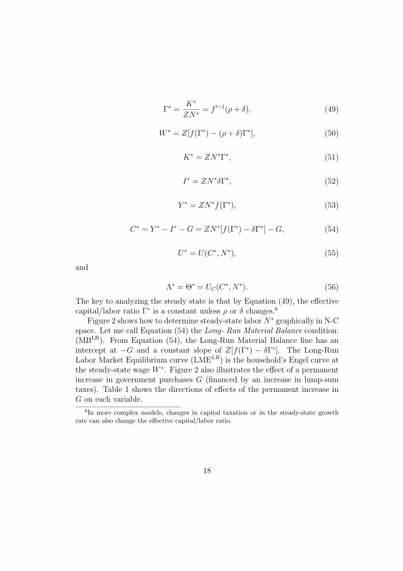
The key to analyzing the steady state is that by Equation (49), the effectivecapital/labor ratio Γ∗ is a constant unless ρ or δ changes.6

Figure 2 shows how to determine steady-state labor N∗ graphically in N-Cspace. Let me call Equation (54) the Long- Run Material Balance condition:(MBLR). From Equation (54), the Long-Run Material Balance line has anintercept at −G and a constant slope of Z[f(Γ∗) − δΓ∗]. The Long-RunLabor Market Equilibrium curve (LMELR) is the household’s Engel curve atthe steady-state wage W ∗. Figure 2 also illustrates the effect of a permanentincrease in government purchases G (financed by an increase in lump-sumtaxes). Table 1 shows the directions of effects of the permanent increase inG on each variable.

6In more complex models, changes in capital taxation or in the steady-state growthrate can also change the effective capital/labor ratio.

18

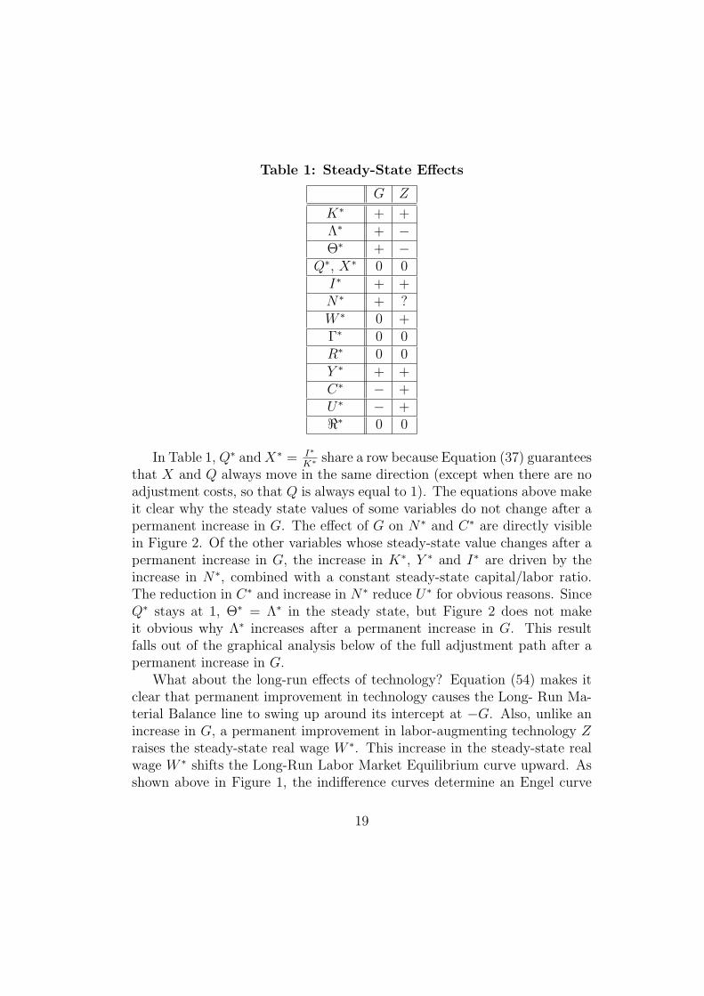
Table 1: Steady-State Effects

G Z

K∗ + +Λ∗ + −Θ∗ + −

Q∗, X∗ 0 0I∗ + +N∗ + ?W ∗ 0 +Γ∗ 0 0R∗ 0 0Y ∗ + +C∗ − +U∗ − +<∗ 0 0

In Table 1, Q∗ and X∗ = I∗K∗ share a row because Equation (37) guarantees

that X and Q always move in the same direction (except when there are noadjustment costs, so that Q is always equal to 1). The equations above makeit clear why the steady state values of some variables do not change after apermanent increase in G. The effect of G on N∗ and C∗ are directly visiblein Figure 2. Of the other variables whose steady-state value changes after apermanent increase in G, the increase in K∗, Y ∗ and I∗ are driven by theincrease in N∗, combined with a constant steady-state capital/labor ratio.The reduction in C∗ and increase in N∗ reduce U∗ for obvious reasons. SinceQ∗ stays at 1, Θ∗ = Λ∗ in the steady state, but Figure 2 does not makeit obvious why Λ∗ increases after a permanent increase in G. This resultfalls out of the graphical analysis below of the full adjustment path after apermanent increase in G.

What about the long-run effects of technology? Equation (54) makes itclear that permanent improvement in technology causes the Long- Run Ma-terial Balance line to swing up around its intercept at −G. Also, unlike anincrease in G, a permanent improvement in labor-augmenting technology Zraises the steady-state real wage W ∗. This increase in the steady-state realwage W ∗ shifts the Long-Run Labor Market Equilibrium curve upward. Asshown above in Figure 1, the indifference curves determine an Engel curve

19

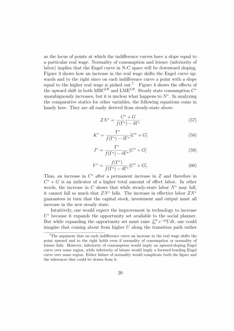
as the locus of points at which the indifference curves have a slope equal toa particular real wage. Normality of consumption and leisure (inferiority oflabor) implies that the Engel curve in N-C space will be downward sloping.Figure 3 shows how an increase in the real wage shifts the Engel curve up-wards and to the right since on each indifference curve a point with a slopeequal to the higher real wage is picked out.7 Figure 4 shows the effects ofthe upward shift in both MBCLR and LMELR. Steady state consumption C∗

unambiguously increases, but it is unclear what happens to N∗. In analyzingthe comparative statics for other variables, the following equations come inhandy here. They are all easily derived from steady-state above.

ZN∗ =C∗ + G

f(Γ∗)− δΓ∗(57)

K∗ =Γ∗

f(Γ∗)− δΓ∗[C∗ + G] (58)

I∗ =Γ∗

f(Γ∗)− δΓ∗[C∗ + G] (59)

Y ∗ =f(Γ∗)

f(Γ∗)− δΓ∗[C∗ + G]. (60)

Thus, an increase in C∗ after a permanent increase in Z and therefore inC∗ + G is an indicator of a higher total amount of effect labor. In otherwords, the increase in C shows that while steady-state labor N∗ may fall,it cannot fall so much that ZN∗ falls. The increase in effective labor ZN∗

guarantees in turn that the capital stock, investment and output must allincrease in the new steady state.

Intuitively, one would expect the improvement in technology to increaseU∗ because it expands the opportunity set available to the social planner.But while expanding the opportunity set must raise

∫∞0 e−ρtUdt, one could

imagine that coming about from higher U along the transition path rather

7The argument that on each indifference curve an increase in the real wage shifts thepoint upward and to the right holds even if normality of consumption or normality ofleisure fails. However, inferiority of consumption would imply an upward-sloping Engelcurve over some region, while inferiority of leisure would imply a forward-bending Engelcurve over some region. Either failure of normality would complicate both the figure andthe inferences that could be drawn from it.

20

than from a higher steady-state U∗. To show that U∗ does increase as onewould expect, decompose the change in N∗ and C∗ into the movement outalong the original Engel curve, which clearly increases U∗, and the movementalong the new Material Balance line. The slope of the Long-Run MaterialBalance line, Z[f(Γ∗)− δΓ∗] is greater than the slope W ∗ = Z[f(Γ∗)− (ρ +δ)Γ∗] of the indifference curves along the corresponding Engel curve. Theslope of the new, steeper, Material Balance line is higher than the slope ofall the indifference curves it intersects in the segment between the two Engelcurves. Therefore, the movement out along the new Material Balance linealso increases U∗.

The effect of a permanent improvement in Z on Λ∗ = Θ∗ is, again, mosteasily seen from the graphical analysis below of the full adjustment path.

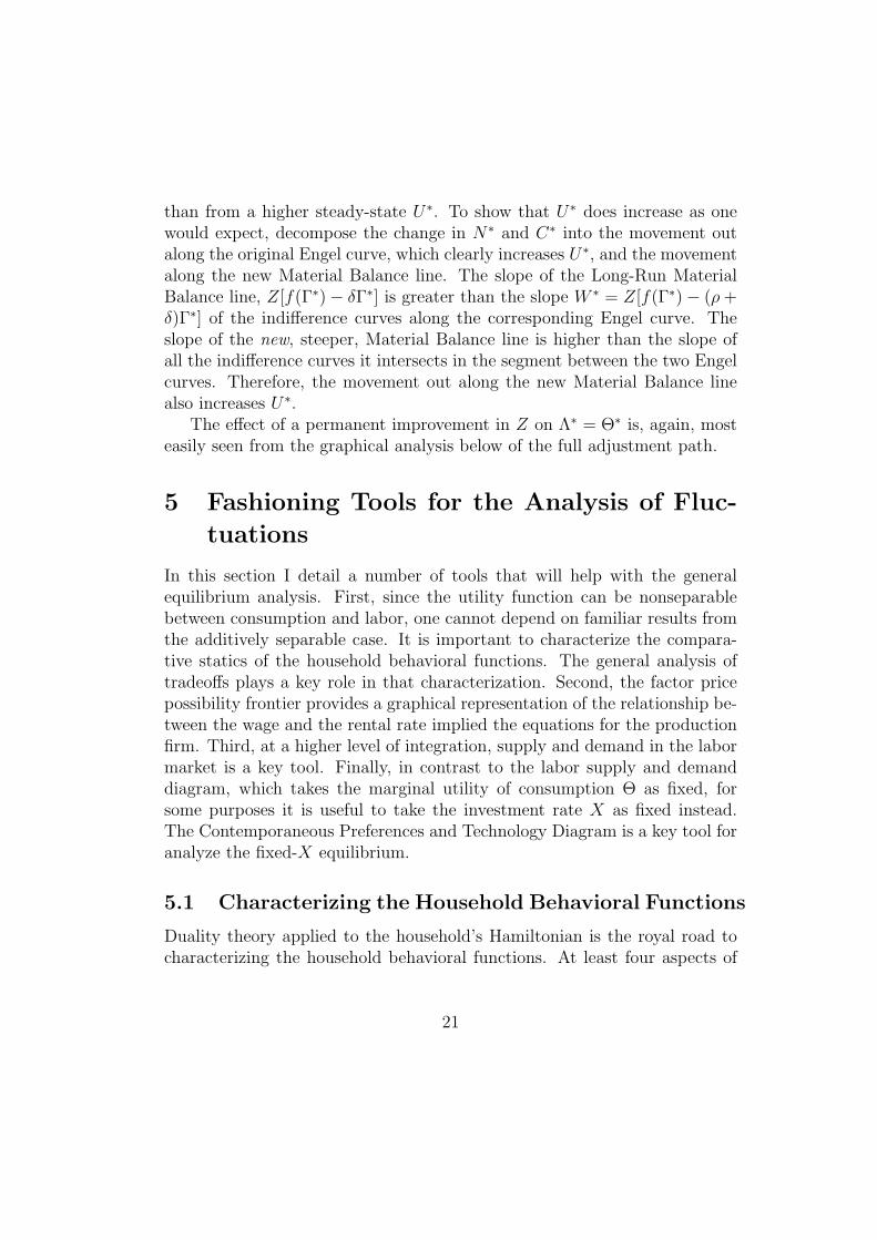
5 Fashioning Tools for the Analysis of Fluc-

tuations

In this section I detail a number of tools that will help with the generalequilibrium analysis. First, since the utility function can be nonseparablebetween consumption and labor, one cannot depend on familiar results fromthe additively separable case. It is important to characterize the compara-tive statics of the household behavioral functions. The general analysis oftradeoffs plays a key role in that characterization. Second, the factor pricepossibility frontier provides a graphical representation of the relationship be-tween the wage and the rental rate implied the equations for the productionfirm. Third, at a higher level of integration, supply and demand in the labormarket is a key tool. Finally, in contrast to the labor supply and demanddiagram, which takes the marginal utility of consumption Θ as fixed, forsome purposes it is useful to take the investment rate X as fixed instead.The Contemporaneous Preferences and Technology Diagram is a key tool foranalyze the fixed-X equilibrium.

5.1 Characterizing the Household Behavioral Functions

Duality theory applied to the household’s Hamiltonian is the royal road tocharacterizing the household behavioral functions. At least four aspects of

21

the household’s behavior are of interest: consumption C, labor hours N ,felicity U , and the household’s primary saving S, defined by

S = WN − C − T. (61)

Define the maximized Hamiltonian H(Θ,W, T ) for the household by

H(Θ, W, T ) = maxC,N

U(C, N) + Θ[WN − C − T ] (62)

Also define the money-metric indicator M by

M = ΥU(C, N) + WN − C − T.

where Υ is the value of a util, and the maximized money- metric indicatorM by

M(Υ,W, T ) = maxC,N

ΥU(C,N) + WN − C − T. (63)

Clearly, when Υ = 1Θ

> 0, the values of C and N that maximize the money-metric indicator M are the same as the values of C and N that maximizethe Hamiltonian H. Clearly, these maximizing values of C and N do notdepend on the lump-sum tax T . Let

(C(Θ,W ), N(Θ,W )) = arg maxC,N

U(C,N) + Θ[WN − C − T ]

= arg maxC,N

Θ−1U(C, N) + WN − C − T. (64)

Also, define

U(Θ,W ) = U(C(Θ,W ), N(Θ,W )) (65)

and

S(Θ,W, T ) = WN(Θ,W )− C(Θ,W )− T (66)

By the envelope theorem,

HΘ(Θ,W, T ) = S(Θ,W, T ), (67)

22

HW (Θ, W, T ) = ΘN(Θ,W ), (68)

and

HT (Θ,W, T ) = −Θ, (69)

MΥ(Υ,W, T ) = U(Υ−1, W ), (70)

MW (Υ,W, T ) = N(Υ−1,W ), (71)

and

MT (Υ,W, T ) = 0. (72)

Thus, the first derivatives of H and M represent the main behavioral out-comes for the household. The second derivatives of H and M convey a greatdeal of information about the determinants of these behavioral outcomes.

Two results allow one to characterize the comparative statics of C, N , Uand S. The first is Young’s Theorem that the order of differentiation doesnot matter for mixed cross-partial derivatives.8 The second is the followinglemma.

Lemma 1 Let F be the real-valued function of the three vectors ξ, β and ζ.If F(ξ, β, ζ) is linear or convex in β, then

F(β, ζ) = maxξF(ξ, β, ζ)

is linear or convex in β. Furthermore, F is strictly convex in β if any changein β forces a change in the optimizing value of ξ, or if F is strictly convexin β. Conversely, F(ξ, β, ζ) is linear in β and a change in β never requiresa change in the optimizing value of ξ, then F is linear in β.

8The limitations on Young’s Theorem that are sometimes emphasized in Calculuscourses are purely technical and have no economic content. In particular, the discretecross-partial of a function φ(x, y) is φ(x+∆x, y+∆y)−φ(x+∆x, y)−φ(x, y+∆y)+φ(x, y),which is symmetric in x and y. The discrete cross-partial carries virtually all the economicmeaning (as has been demonstrated in the literature on monotone comparative statics andsupermodularity), and raises no technical issues.

23

Proof: Given any values for β0 and ζ, let ξ(β0, ζ) maximize F(ξ, β0, ζ).Then for any β1

F(β1, ζ) = maxξF(ξ, β1, ζ)

≥ F(ξ(β0, ζ), β1, ζ)

≥ F(ξ(β0, ζ), β0, ζ) + Fβ(ξ(β0, ζ), β0, ζ)[β1 − β0]

= F(β0, ζ) + Fβ(β0, ζ)[β1 − β0]. (73)

Overall, (73) shows that F is always above its tangent planes in thedimensions represented by β, which guarantees that F is convex in β. Theequalities at the beginning and end are the definition of F . The first inequal-ity follows from the nature of maximization. It is strict if ξ(β0, ζ) does notmaximize F(ξ, β1, ζ). The second inequality is a consequence of F(ξ, β, ζ)being linear or convex in β. It is strict if F is strictly convex in β. If a changein β never requires a change in the optimizing value of ξ and F(ξ, β, ζ) islinear in β, every line of (73) holds with equality.

Figure 5 illustrates the basic idea behind Lemma (1). It shows a casewhere F(ξ, β, ζ) is linear in β and ξ can is chosen from one of three values.F is the convex upper envelope of the three lines.

5.1.1 Applying Lemma 1

Though it is unnecessary for the economic substance, for heuristic purposes,the applications of Lemma (1) below assume that F is twice-differentiable.Typically, such convenient differentiability would require that ξ be chosenfrom a continuum of values, unlike the case in Figure 5.

Applying Lemma 1 to the main diagonals of the Hessians of H and Myields

HΘΘ(Θ,W, T ) = SΘ(Θ,W, T ) ≥ 0, (74)

HWW (Θ,W, T ) = ΘNW (Θ,W, T ) ≥ 0, (75)

24

MΥ,Υ = −Υ−2UΘ(Υ−1, W ) ≥ 0, (76)

and

MWW = NW (Υ−1,W ) ≥ 0. (77)

Looking at HTT or MTT only yields 0 ≥ 0. The meaning of (74) is clear.Both (75) and (77) say that labor supply is increasing in the real wage:NW (Θ,W ) ≥ 0. There is no possibility of a backward-bending labor supplycurve this is a Frisch labor supply curve; holding the marginal utility ofwealth Θ constant blocks most of the power of income effects.

Inequality (76) implies that

UΘ(Θ,W ) ≤ 0. (78)

The intuition for (74) and (78) is made clearer by a simple tradeoff diagram—in this case the felicity-saving possibility frontier shown in Figure 6.

As can be seen from (62) and (61), at any moment the household ismaximizing U + ΘS by choosing the point on the felicity-saving possibilityfrontier with a slope of −Θ. An increase in the marginal value of wealthΘ makes saving relatively more important compared to the current flow ofutility and causes the household to choose a point further down to the right,with higher primary saving S and lower felicity U . Though it is less nat-ural, one can draw a similar tradeoff diagram to give additional intuitionfor the result NW (Θ,W ) ≥ 0. The money-metric indicator can be writ-ten [ΥU(C, N) − C − T ] + WN . Putting N on the horizontal axis andΥU(C, N) − C − T on the vertical axis, the possibility frontier in Figure7 picks out points that maximize ΥU(C, N)− C − T , money-metric felicitynet of consumption and taxes, for each value of N . Other values of C yieldpoints inside the possibility frontier. The money-metric indicator is maxi-mized where the possibility frontier in Figure 7 has slope equal to −W . Ahigher real wage W causes the household to choose a point further down tothe right, with higher N and lower net felicity ΥU(C, N)− C − T .

5.1.2 Applying Young’s Theorem

Applying Young’s theorem to HΘT only confirms that ST (Θ,W, T ) = −1,while if I had not already argued that C, N and U do not depend on

25

T , applying Young’s theorem HTW , MTΥ, MTW would only confirm thatNT (Θ,W, T ) = 0 and UT (Θ,W, T ) = 0. Note that

C = WN − S − T

so that CT would be

CT (Θ,W, T ) = WNT (Θ,W, T )− ST (Θ,W, T )− 1 = 0,

confirming that, given Θ and W , consumption is not a function of the currentflow of lump sum taxes. This is a reflection of Ricardian equivalence.

Applying Young’s theorem to HΘW yields

SW (Θ,W, T ) = N(Θ,W ) + ΘNΘ(Θ,W ) (79)

Substituting into (79) the identity S(Θ,W, T ) = WN(Θ,W )− C(Θ,W )−Tyields

N(Θ,W ) + WNW (Θ, W )− CW (Θ,W ) = N(Θ,W ) + ΘNΘ(Θ,W )

or equivalently,

WNW (Θ,W )− CW (Θ,W ) = ΘNΘ(Θ,W ). (80)

Applying Young’s theorem to MΥW yields

UW (Υ−1,W ) = −Υ−2NΘ(Υ−1,W ),

implying

UW (Θ,W ) = −Θ2NΘ(Θ, W ). (81)

Since UΘ(Θ,W ) ≥ 0, normality of leisure, or equivalently, inferiority oflabor, implies that NΘ(Θ,W ) > 0. (Normality and inferiority have to dowith what happens as one moves to a higher indifference curve holding thereal wage W constant.) By (80) and (81), normality of leisure and inferiorityof labor imply

WNW (Θ,W )− CW (Θ,W ) > 0 (82)

26

and

UW (Θ, W ) < 0. (83)

Inequality (82)—or equivalently both sides of (79) being positive—can beinterpreted as saying that an increase in the real wage will affect saving bymore than the direct effect of the wage on household income for constant N .In other words, an increase in the real wage will raise quantitative savingeffort in terms of N and C. This increase in quantitative saving effort isassociated with a fall in the current flow of utility indicated by (83). Notethat, mechanically, holding Θ constant blocks most income effects, throughwhich one might otherwise expect an increase in the real wage to raises thehousehold’s felicity. If nothing else changes, a temporary increase in the realwage will indeed make the household better off, but only by raising futurefelicity. At the moment, the household will be working too hard to enjoythemselves.

Graphically, thinking about the shift in the felicity-saving possibility fron-tier due to an increase in the real wage W provides the intuition for (83) and(82). For given values of C and N , an increase in the real wage raises pri-mary saving by NdW . Thinking in terms of small changes, the envelopetheorem guarantees that in Figure 8, for given U , the value of S on thefelicity-saving possibility frontier shifts right by N(Θ,W )dW . Inferiority oflabor implies that N is highest at points low down to the right on the felicity-saving possibility frontier, where U is low. Therefore, an increase in W shiftsthe felicity-saving possibility frontier further to the right at lower values ofU . As Figure 8 illustrates, this makes the new felicity-saving possibility fron-tier flatter than the old one at the corresponding point directly to the right.Thus, the point on the new felicity-saving possibility frontier that has theunchanged slope −Θ must be lower down on the new possibility frontier: theincrease in W , holding Θ fixed reduces the optimal value of U , confirming(83). This movement down along the felicity-saving possibility frontier guar-antees in turn that primary saving will increase by more than the rightwardshift of the possibility frontier N(Θ,W )dW—which is the essence of (82).

27

5.1.3 Summarizing the Characterization of Household BehavioralFunctions

At this point we can sign (at least in the weak sense) all but one of thederivatives of C, N , U and S:

C ( Θ

−, W

?

);

N ( Θ

+

, W

+

);

U ( Θ

−, W

−);

S ( Θ

+

, W

+

, T

−)

(84)

The negative effect of Θ on consumption is due to normality of consumption.The effect of W on consumption remains to be discussed.

The positive effect of Θ on labor is due to normality of leisure, or equiv-alently, inferiority of labor. The normality of leisure or inferiority of laboralso implies the negative effect of W on felicity U through Young’s theorem.

The positive effect of W on labor, the negative effect of Θ on felicity Uand the the positive effect of Θ on saving all reflect the monotone compara-tive statics principle that the optimal quantity of something goes up when itsweight in the objective function increases—and conversely that the optimalquantity of something goes down when its weight in the objective functiondeclines. This principle is a special case of the principles surrounding super-modularity and submodularity, to be discussed below.

Finally, the negative effect of lump-sum taxes T on saving reflects thefact that consumption and labor are unaffected by lump-sum taxes, given Θand W—a fact closely connected to Ricardian equivalence.

5.1.4 The Effects of Nonseparability Between Consumption andLabor

What determines the sign of the effect of the real wage on consumption?Looking at the problem of maximizing the household’s Hamiltonian,

maxC,N

U(C, N) + Θ[WN − C − T ]

the real wage does not interact directly with consumption. However, laborpotentially interacts with consumption in U(C,N), and so the real wage canaffect C through its effect on N . Because an increase in W , holding Θ fixedunambiguously raises N , the sign of the effect of W on C is determined by

28

the sign of the cross-partial UCN . If UCN > 0, then the increase in N inducedby higher W raises the optimal level of C. If UCN < 0, then the increase inN induced by higher W lowers the optimal level of C. Finally, in the famil-iar (but not necessarily realistic) additively- separable case, UCN = 0, theincrease in N induced by higher W has no effect on the optimal level of C.All of these statements follow from the basic principles of supermodularity.UCN > 0 makes the Hamiltonian supermodular in consumption and labor;UCN < 0 makes the Hamiltonian submodular in consumption and labor;and UCN = 0 makes the Hamiltonian modular in consumption and labor.Because of the concavity and differentiability assumptions I have made, thesituation is simpler than the usual situation to which supermodularity prin-ciples are applied. In this case, one can focus on the first-order condition forconsumption

UC(C, N) = Θ.

Figure 9 shows the case in which UCN > 0. The increase in N induced by ahigher real wage shifts UC(C,N) upwards for every value of C. Therefore, thepoint at which UC(C,N) crosses the marginal value of wealth line, horizontalat Θ, is pushed further to the right. If UCN < 0 the marginal utility ofconsumption curve is pushed down by the increase in N and the intersectionwith the horizontal marginal value of wealth line would be shifted to the left.Additive separability would make N irrelevant to the figure.

Basu and Kimball (2002) argue that UCN should be positive because thispreserves equality of income and substitution effects on labor supply whenthe elasticity of intertemporal substitution for consumption is less than one.In particular, King, Plosser and Rebelo (1988) show that to keep hours perworker and the real interest rate constant under conditions of steady-stategrowth, U(C, N) must be of the form

U(C, N) =C1−(1/s)

1− (1/s)Ω(N), (85)

where s 6= 1 is the elasticity of intertemporal substitution, or

U(C, N) = ln(C)− v(N) (86)

when s = 1. Although Equation (86) is convenient, empirical evidence points

29

to a value of s significantly less than one.9 A variety of empirical evidence alsopoints directly to UCN > 0. Basu and Kimball (2002) look at the aggregateevidence directly and discuss the literature on the micro evidence.

5.2 The Factor-Price Possibility Frontier

As illustrated in Figure 10, Equations 88 and 22 define the Factor-PricePossibility Frontier parametrically with

(W,R) = (Z[f(Γ)− Γf ′(Γ)], f ′(Γ)), (87)

where Γ = KZN

is the parameter. The labor- augmenting technology Z is theonly thing that shifts the factor price possibility frontier. Straightforwardcalculation shows that the slope of the Factor Price Possibility frontier isequal to − 1

ZΓ= −N

K, which is closer to zero when R/W is higher. Therefore,

the factor price possibility frontier is always convex as shown, becoming linearin the case of Leontieff technology.

The Factor Price Possibility Frontier serves as a graphic reminder thatthe real wage and the real rental rate must always move in opposite directionsunless technology changes. This has to do with both constant returns to scaleand the constancy of the markup ratio P

MC≡ 1.

5.3 Labor Supply and Demand

Figure 11 shows labor supply and demand. N = N(Θ,W ) is the labor supplyequation. The labor supply curve is upward sloping because N(Θ,W ) ismonotonically increasing in W .10 An increase in Θ shifts the labor supplycurve to the right because of the normality of leisure. The marginal utilityof consumption Θ is a summary statistic for everything that shifts the laborsupply curve, since it is the only other variable that appears in N(Θ,W ).

In other words, given Θ, nothing else shifts the labor supply curve. Equa-tion (88) is the labor demand equation. Letting W d(N,K,Z) be the wagedetermined by labor demand,

W d(N, K, Z) = Z[f

(K

ZN

)−

(K

ZN

)f ′

(K

ZN

)]. (88)

9See for example Hall (1988) and Barsky, Juster, Kimball and Shapiro (1997).10See (75) or (77).

30

The original assumption that the production function is supermodular inlabor and technology implies

FKZ = W dZ(N, K, Z) ≥ 0. (89)

The other two derivatives are

W dN(N,K,Z) =

(K2

ZN3

)f ′′

(K

ZN

)< 0. (90)

W dK(N, K, Z) = −

(K

ZN2

)f ′′

(K

ZN

)> 0. (91)

Equation (90) implies that the labor demand curve is downward sloping.Equations (91) and (90) imply that both K and Z shift the labor demandcurve upward and outward. Given K and Z, no other variable has any effecton the labor demand curve.

For fluctuations, as for the steady-state, given labor hours N , many othervariables can be determined recursively. Thus, the interaction between laborsupply and demand that determines N nonrecursively is a central part ofthe model’s mechanism. For use in higher levels of integration in the model,define W(Θ, K, Z) as the equilibrium real wage and N (Θ, K, Z) equilibriumquantity of labor determined in the labor market.

5.4 The Contemporaneous Preferences and Technol-ogy Diagram

The Contemporaneous Preferences and Technology Diagram is illustrated inFigure 12. The Contemporaneous Preferences and Technology Diagram takesthe investment rate X as fixed. Given X, the Contemporaneous MaterialBalance (CMB) curve is

C = F (K, N,Z)−XK −G = ZNf(

K

ZN

)−XK −G. (92)

The Contemporaneous Material Balance curve is upward sloping and concavein N -C space since FN > 0 and FNN < 0.

Since any point on the Contemporaneous Material Balance curve allowsthe same level of government purchases and investment I = XK for the fu-ture, all points are equally good as far as the future is concerned. Therefore,

31

given K and X, the social planner should maximize current felicity U . Inother words, a characteristic of the overall solution to the social planner’sproblem must be that, whatever the optimal value of K and X at any mo-ment, along with the exogenous values of Z and G, the social planner will putthe economy at the highest level of felicity available along the Contempora-neous Material Balance curve. Of course, the highest level of U is achieved atthe point at which the Contemporaneous Material Balance curve is tangentto an indifference curve at that point.

Because of the tangency condition, in the Contemporaneous Preferencesand Technology Diagram, both the level and the slope of the curves matter.The comparative statics of the level and slope of the Contemporaneous Ma-terial Balance curve can be seen from Equation (92). An increase in eitherX or in G shifts the Contemporaneous Material Balance curve downward ina parallel shift that does not change the slope at a given level of G. Becauseof the assumption that FZN > 0, an increase in Z raises both the level andslope of the Contemporaneous Material Balance curve at a given level ofN . An increase in the capital stock raises the level of the ContemporaneousMaterial Balance curve at a given level of N as long as

FK −X = R−X > 0,

and always raises the slope of the Contemporaneous Material Balance curveat a given N .

Since I am abstracting from preference shocks that would change theshape of felicity U(C, N) the indifference curves do not shift. Indeed, theindifference curves are invariant to shocks to impatience ρ as well.

On the household’s side, the real wage in the tangency condition is de-termined by a function W (C, N):

W =−UN(C, N)

UC(C, N)

= W ( C

+

, N

+

). (93)

Equations (3) and (4) imply that W (C,N) is increasing in both arguments.In particular, moving up along the Contemporaneous Material Balance curvethe needed wage on the household side, W (C,N), increases, while the wage

32

at which the firm demands labor FN(K,N, Z) = W d(K, N, Z) decreaseswith the increase in N . Thus, if a particular point on the ContemporaneousMaterial Balance curve has FN(K, N, Z) > W (C, N), then the tangencypoint must be further up along the Contemporaneous Material Balance curve.Conversely, if a particular point on the Contemporaneous Material Balancecurve has FN(K,N, Z) < W (C,N), then the tangency point must be lowerdown along the Contemporaneous Material Balance curve.

The direction of movement of labor N , consumption C, the real wageW and felicity U are readily apparent in the Contemporaneous Preferencesand Technology Diagram. It is also not too hard to use the behavior of Wand N to determine what is happening to the rental rate R, the effectivecapital/labor ratio Γ = K

ZNand output Y . With X fixed, the behavior of Λ

will turn out to depend primarily on the rental rate R. Less obviously, theContemporaneous Preferences and Technology Diagram indicates a fair bitabout the movement of the marginal utility of consumption Θ. First, thereis the direct dependence of UC(C, N) on C and N according to UCC < 0 andUCN , which can be of either sign as discussed above. Second, the equation

U = U(Θ,W ) (94)

can be inverted in its first argument to yield the function Θ(U,W ).

Θ ( U

−, W

−). (95)

Holding W fixed, the negative effect of Θ on U in U(Θ,W ) implies a negativeeffect of U on Θ in the inverted function Θ(U,W ). When the real wage Wincreases, the direct effect on U in Equation (94) is negative. The value ofU in Equation (94) can be held fixed by reducing Θ as W increases. Thisreduction of Θ along with W in order to hold U fixed in Equation (94)corresponds to a negative effect of W on Θ in Equation (95) when holdingU fixed.

There is another way to see why normality of leisure, which is behindthe negative effect of W on U(Θ,W ), implies that W has a negative effecton Θ(U,W ). As shown in Figure 1, normality of leisure corresponds to thepositive effect of C on W (C,N). If the point on an indifference curve directlyabove another point has a higher slope, then the vertical distance betweenindifference curves must increase as one follows both indifference curves to

33

the right. With the gap in felicity U fixed by a focus on these two indifferencecurves, the increasing vertical distance implies that in comparing these pairsof points, ∆C

∆Uis increasing as we follow both indifference curves up to the

right. Then it only requires focusing on very close indifference curves to seethat

Θ =∂U

∂C= lim

∆U→0

(∆C

∆U

)−1

is decreasing as we follow an indifference curve around to the right, whereW is higher.

6 Contemporaneous General Equilibrium

The QRBC model, and any similarly complex dynamic general equilibriummodel has at least four levels of integration:

1. Household and Firm Optimization

2. Market Equilibrium

3. Contemporaneous General Equilibrium

4. Dynamic General Equilibrium.

Household and firm optimization are clear concepts. Labor market equi-librium is a good example of what I mean by the market equilibrium level ofintegration.

Contemporaneous general equilibrium is the least familiar concept. Con-temporaneous general equilibrium is defined as the solution to the modelwhen the current values of the endogenous state variables, costate variablesand exogenous variables are taken as given. It is a very useful concept be-cause the structure of contemporaneous general equilibrium is invariant tothe time- series properties of the exogenous variables. The structure of con-temporaneous general equilibrium makes the endogenous state variable(s) asufficient statistic for the past and the costate variable(s) a sufficient statisticfor the future, so that these plus the current values of the exogenous vari-ables are enough to determine contemporaneous general equilibrium. In the

34

QRBC, this means that the current values of K, Λ, Z and G are enough todetermine all of the other key variables except the real interest rate. The realinterest rate < is not determined in contemporaneous general equilibrium; inthe QRBC model, it is by nature a dynamic general equilibrium object.

Even in an exact solution to a dynamic stochastic general equilibriummodel, without linearization or a certainty- equivalence approximation, thestructure of contemporaneous general equilibrium is invariant to the stochas-tic processes of the exogenous variables.

Dynamic general equilibrium is the overall outcome of the model. In theQRBC model, there is only one endogenous state variable, so the dynamicsof K and Λ in dynamic general equilibrium can be illustrated by a two-dimensional phase diagram. In a linearized or log-linearized model, usinga certainty-equivalence approximation, the essential structure of dynamicgeneral equilibrium is given by the impulse responses of all the key variablesto each relevant type of shock.

To understand the model, it is useful to think of each point on the phasediagram not just as a (K, Λ) pair that determines a dynamic arrow (K, Λ),but as a particular contemporaneous general equilibrium that determinesmany other variables of interest at the same time as it determines K and Λ.Contemporaneous general equilibrium is the key to determining the mappingfrom (K, Λ) to (K, Λ) that governs the phase diagram dynamics.

The structure of contemporaneous general equilibrium means that the im-pulse responses of K and Λ that come out of the phase diagram, combinedwith the impulse responses of Z and G, generate impulse responses for all ofthe other variables determined as functions of K, Λ, Z and G in contempora-neous general equilibrium. In a more intricate way, these impulse responsesalso allow one to determine the impulse response of the real interest rate <.

In the Ramsey-Cass-Koopmans model that is often used to teach the useof phase diagrams with dynamic general equilibrium models, contemporane-ous general equilibrium is trivial, but contemporaneous general equilibriumis not trivial in the QRBC model. Because the concept of contemporane-ous general equilibrium is relatively unfamiliar, its behavior may not alwaysseem intuitive. In particular, holding the marginal value of capital Λ fixedcan seem as unnatural in its own way as holding price fixed to think aboutshifts in the supply and demand curves often seems to students in “Princi-ples of Economics,” who often have more intuition for market equilibrium(at least in simple cases) than for the analytical constructs of supply and

35

demand that economists use to think about market equilibrium.In the QRBC model, the analysis of contemporaneous general equilibrium

is closely linked to the analysis of equilibrium between investment demandand saving supply, since it is straightforward to determine the values of all theother variables in contemporaneous general equilibrium once the investmentrate and the marginal utility of consumption are determined by investmentdemand and saving supply. But before moving on to investment demand andsaving supply, there is some housekeeping to do.

6.1 Taking logarithms of the dynamic variables

Equations (12), (17), (28) and (33), suggest that it is convenient to expressthe dynamic equations of the QRBC model and its partial equilibrium in

terms of logarithmic time derivatives: KK

, ΛΛ, Θ

Θand Q

Q. Using small letters

for logarithms, these equations can be rewritten

k = J(X), (96)

λ = ρ− J(X)− J ′(X)[R−X], (97)

θ = ρ−<, (98)

and

q = <− J(X)− J ′(X)[R−X]. (99)

Note that Equation (97) has the same form as Equation (99), except thatthe real interest rate is replaced by the utility discount rate. Thus, Equation(97) also admits of a required-rate-of-return interpretation, but with utils asthe numeraire instead of dollars:

ρ =RK − I

QK+ k + λ. (100)

I will resist the temptation to fully log-linearize the model here, sincethat would take things in a different direction, toward quantitative analyt-ics. But even in studying the qualitative analytics in a way that allows forthe nonlinearities in contemporaneous general equilibrium and at least the

36

perfect- foresight version of dynamic general equilibrium,11 it is convenientto analyze the dynamics in terms of the logarithms k, λ, θ and q. Of course,every comparative static statement about Θ in the discussion of householdbehavioral functions applies equally well to θ and every comparative staticstatement about K in the discussion of labor demand applies equally well tok.12

6.2 The Investment Demand Curve

It works well to analyze investment demand and saving supply in X-θ space.On the horizontal axis, this means thinking about investment and saving inrelation to the preexisting size of the capital stock. It makes sense to put(log) marginal utility θ on the vertical axis because θ is central to householdbehavior and therefore to saving supply.

Defining the function q(X) by

q(X) = − ln(J ′(X)), (101)

Equation (39) can be rewritten as

θ = λ− q(X). (102)

Equation (102) is the investment demand (II) curve. As illustrated in Figure13, the investment demand curve intersects the vertical line X = δ at thelevel λ. The investment demand curve is downward sloping since q(X) isincreasing in X. An increase in λ causes a parallel upward shift in theinvestment demand curve. In X-θ space the (log) marginal value of capitalλ is a sufficient statistic for everything that shifts the investment demandcurve.13

11This can be useful: Kimball (1993) shows how to use the nonlinearities in a per-fect foresight model to derive a perturbation-theory approximation to dynamic stochasticgeneral equilibrium.

12However, the derivations of many of these comparative statics results were made easierby the use of K and Θ rather than k and θ.

13In I-θ space, an increase in k would shift the investment demand curve out and up.

37

6.3 Saving Supply

Saving supply can be thought of either as a function of Θ, K, Z and G,through the lens of Fixed-Θ equilibrium, or as a function of X, K, Z andG, through the lens of Fixed-X equilibrium. Both Fixed-Θ equilibrium andFixed-X equilibrium are important for analyzing the comparative statics ofContemporaneous General Equilibrium, which always lie between the com-parative statics for the Fixed- Θ and the comparative statics for the Fixed-Xequilibria. The Fixed-Θ equilibrium corresponds to the ContemporaneousGeneral Equilibrium when J(X) = X − δ, so that there are no investmentadjustment costs. Conversely, very large investment adjustment costs makeContemporaneous General Equilibrium behave much like Fixed-X equilib-rium. Intermediate degrees of adjustment costs make Contemporaneous Gen-eral Equilibrium something in between.

For clarity, let me say that in naming “Fixed-Θ” or “Fixed-X” equilib-rium, I am using “fixed” in the sense of “stipulated,” “specified” or “known,”rather than in the sense of “unchanging.” Fixed-Theta equilibrium, for ex-ample, is what one gets by treating the marginal utility of consumption Θ asif it were exogenous, while Fixed-X equilibrium is what one gets by treatingthe investment rate X as if it were exogenous. In both cases, K is treatedas if it were exogenous, which is natural for the analysis of a single point intime. Implicitly, if either Θ or X is treated as if it were exogenous, Λ mustbe treated as endogenous. Thus, on the phase diagram, Fixed-Θ Equilibriumpicks out an iso-Θ locus. The effect of a change in K on Fixed-Θ equilib-rium shows up as a movement along the iso-Θ locus, while the effects of achange in Z or G show up as a shift of the iso-Θ locus. Varying Θ picks outa different iso-Θ locus. Similarly, Fixed-X Equilibrium picks out an iso-Xlocus. Some of the importance of Fixed-X equilibrium comes from that factthat iso-X locus with X = δ is the k = 0 locus.

6.3.1 Fixed-Marginal-Utility-of-Consumption Equilibrium

Gross national saving is Y −C −G. This is not the same as the household’sprimary saving S. The relationship is

Y − C −G = S + RK + T −G.

Remember that primary saving S does not include interest income or debt

38

payments. Define the function X (Θ, K, Z, G) by

X (Θ, K, Z, G) =F (K,N (Θ, K, Z), Z)− C(Θ,W(Θ, K, Z))−G

K, (103)

where N and W give the labor market equilibrium values of labor and thereal wage. Then the saving supply curve, which focuses on gross nationalsaving relative to the capital stock, is given by

X =Y − C −G

K= X (Θ, K, Z, G) = X (eθ, ek, Z, G).

It is clear from Equation (103) that saving supply is intimately boundup with labor supply and demand. The four variables Θ, K, Z and Gthat determine saving supply are also enough to determine the values ofN = N (Θ, K, Z), W = W(Θ, K, Z),

Γ =K

ZN (Θ, K, Z), (104)

R = f ′(

K

ZN (Θ, K, Z)

), (105)

C = C(Θ,W(Θ, K, Z)), (106)

U = U(Θ,W(Θ, K, Z)), (107)

Y = (K,N (Θ, K, Z), Z), (108)

I = KX (Θ, K, Z,G), (109)

k =K

K= J(X (Θ, K, Z, G)) (110)

39

λ =Λ

Λ= ρ− J(X (Θ, K, Z, G))

−J ′(X (Θ, K, Z, G))[f ′(

K

ZN (Θ, K, Z)

)−X (Θ, K, Z, G)] (111)

The comparative statics for all of these variables in labor market equilib-rium are given in Table 2.14 In addition to the assumptions in Section 2, theeffect of K on X, and the effect of G on λ depend on being close enough tothe steady state.

Table 2: Fixed-Marginal-Utility-of-ConsumptionComparative Statics

Θ K Z G

λ + + + −N + + + 0W − + + 0Γ − + − 0R + − + 0Y + + + 0C − ? ? 0U − − − 0I + + + −

X, q, k + + + −λ ? + + −

Let me spell out the reasons for each of these signs, beginning with theeffects of an increase in marginal utility Θ for fixed K, Z and G.

As mentioned above, treating Θ as exogenous means that λ will have tovary. By Equation (102),

λ = θ + q(X). (112)

14Given the additional assumption UCN > 0, which I favor, the effects of K and Z areunambiguously positive.

40

Therefore, holding θ constant, λ must move in the same direction as q andX. The last three signs in the row for λ are copied from those in the rowfor X. The logic for the direction of effects on X in Fixed-Θ equilibrium aregiven below. When Θ increases, holding K, Z and G constant, q and X turnout to increase as well, so the required value of λ goes up. This accounts forthe upper-left-hand sign in Table 2.

Θ ↑: As shown in Figure 14, an increase in marginal utility Θ (or equiva-lently, an increase in log marginal utility θ) shifts the labor supply curve outwith no effect on labor demand, raising labor N and lowering the real wageW . The increased N lowers the effective capital labor ratio Γ; the relativeshortage of capital raises the rental rate R.

Because felicity may not be additively separable in consumption and la-bor, it is not as obvious why consumption falls with an increase in Θ as onemight think. Figure 15 shows why consumption falls in response to anincrease in Θ, regardless of the sign of UCN . The lower real wage W shiftsthe relevant Engel curve downward. Combined with the rightward shift inN , this guarantees that consumption must fall. Note that the normality ofconsumption and leisure are important for this argument, since an upward-sloping or forward-bending Engel curve would undercut the argument.

Felicity U falls because labor goes up and consumption goes down. Out-put increases because labor increases, with K and Z fixed. Since output in-creases, while consumption falls, I = Y −C −G goes up, as does X = I/K,since K is fixed. The increase in the investment rate X raises the growthrate of the capital stock k in a mechanical way and must reflect an increasein Tobin’s q.

The effect of an increase in Θ on λ is ambiguous because there are twoopposing effects. Taking a total differential of both sides of Equation (97),

d(λ) = −J ′′(X)[R−X]dX − J ′(X)dR. (113)

Using Equation (100) to aid in interpretation, the first term the reductionin the rate of return when Q increases along with X. A higher util capitalgains rate λ can help meet the required rate of return. The direct costs andbenefits of X cancel out because of the leasing-firm’s first-order condition,Equation (32). The last term, −J ′(X)dR, reflects the ability of a higherrental rate to meet the required rate of return as an alternative to a higherutil capital gains rate λ.

41

In response to an increase in Θ, the rental rate R increases, so the secondterm −J ′(X)dR will be negative. As for the first term, since X∗ = δ, whileR∗ = ρ + δ, anywhere reasonably close to the steady-state R − X will bepositive, so −J ′′(X)[R −X] will be positive. Since the increase in Θ raisesX, the entire first term −J ′′(X)[R − X]dX is positive. Thus, the effectof an increase in Θ on λ is ambiguous. If investment adjustment costs aresmall, then −J ′′(X) will be small and the λ will fall when Θ increases. Ifinvestment adjustment costs are large, then −J ′′(X) will be large and λ mayfall when Θ increases. This cannot be ruled out, since neither X (Θ, K, Z, G),nor the determination of R in Equation (105) are affected by the shape ofthe accumulation function J .

K ↑: As shown in Figure 16, an increase in capital K (or equivalently,an increase in the log of the capital stock k) shifts labor demand out withno effect on labor supply. The outward shift in labor demand increases bothlabor N and and the real wage W . The increase in both productive factorsK and N raises output Y .

As shown in Figure 17, the Factor Price Possibility Frontier implies thatthe increase in the real wage W must correspond to a decrease in the rentalrate R. Since R = f ′(Γ), this decreasing in the rental rate has to come froman increase in the capital to effective labor ratio Γ = K

ZN.

With Θ fixed, felicity U falls because because the increase in K raises thereal wage W , and UW (Θ,W ) ≤ 0. (See Figure 8.)

As for consumption C, as shown in Figure 9, in my preferred case UCN > 0(supermodularity between consumption and labor), CW (Θ,W ), so the in-crease in the real wage induced by an increase in the capital stock reducesconsumption. However, the claim that UCN > 0 is more controversial thanthe assumptions I made in Section 2, so the entry in Table 2 shows a questionmark to account for the possibility that UCN < 0, which would reverse thesign of CW and cause C to fall when K increases.

The strong possibility that consumption rises when K increases, holdingΘ fixed makes it more difficult to sign the change in I and X = I

K. Totally

differentiating expressions for I and X yields

42

dI = d(Y − C −G)

= FK(K, N, Z)dK + FZ(K,N, Z)dZ − dG

+[FN(K,N, Z)NΘ(Θ,W )− CΘ(Θ,W )]dΘ

+[FN(K,N, Z)NW (Θ,W )− CW (Θ,W )]dW

= RdK + FZ(K,N, Z)dZ − dG

+[WNΘ(Θ, W )− CΘ(Θ,W )]dΘ

+[WNW (Θ,W )− CW (Θ,W )]dW

and

dX = dY − C −G

K

= [R−X]dK

K+

FZ(K,N, Z)dZ − dG

K

+[WNΘ(Θ,W )− CΘ(Θ,W )]dΘ

K

+[WNW (Θ,W )− CW (Θ,W )]dW

K.

In this column of Table 2, Θ, Z and G are held constant. Inequality (82)guarantees that WNW − CW ≥ 0, so the increase in the real wage inducedby a higher capital stock brings forth more saving effort from the household.This, combined with the direct increase in output represented by the term[R −X]dK

Kguarantees a higher level of investment. For the investment rate

X the story is similar, but slightly more complex. Since R∗ − X∗ = ρ, thefactor R −X is positive for some range around the steady state. Of course,q and k increase along with X.

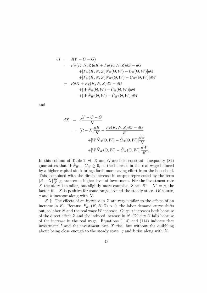
Z ↑: The effects of an increase in Z are very similar to the effects of anincrease in K. Because FKZ(K, N,Z) > 0, the labor demand curve shiftsout, so labor N and the real wage W increase. Output increases both becauseof the direct effect Z and the induced increase in N . Felicity U falls becauseof the increase in the real wage. Equations (114) and (114) indicate thatinvestment I and the investment rate X rise, but without the quibblingabout being close enough to the steady state. q and k rise along with X.

43

As with an increase in K, the change in consumption C is driven by thechange in the real wage. The direction of the effect on consumption is givenby the sign of CW (Θ,W ), which in turn is the same as the sign of UCN . In mypreferred case, UCN > 0, the improvement in technology causes consumptionto rise for fixed Θ.

The one big difference between an increase in K and an increase in Z isthat the increase in Z shifts the factor price possibility frontier out, as shownin Figure 18. The rental rate R increases as well as the real wage W becausewith both Z and N increasing, Γ = K

ZNmust fall and so f ′(Γ) must rise.

G ↑: Holding Θ, K and Z fixed, an increase in government purchases hasno effect on either labor supply or labor demand. Thus, nothing happensto N or W . Since K, N and Z are unchanged, Γ = K

ZN, R and Y are all

unchanged.With both marginal utility Θ and the real wage W unchanged, C =

C(Θ,W ) and U = U(Θ,W ) are unchanged.With output and consumption unchanged, I = Y − C − G and X = I

K

both fall, accompanied by q and k.Finally, with R unchanged and X lower, Equation (113) implies that λ

decreases as long as R−X > 0. Again, since R∗ −X∗ = ρ, R−X > 0 in asubstantial region around the steady-state.

What is happening is that holding marginal utility Θ constant zeroes outwealth effects and interest-rate effects on household behavior, leaving onlythe direct effect of government purchases on X because of economy-widematerial balance, and the consequences of a lower investment rate for q andthe rate of return.

6.3.2 Fixed-Θ Equilibrium and the Comparative Statics of theSaving Supply Curve

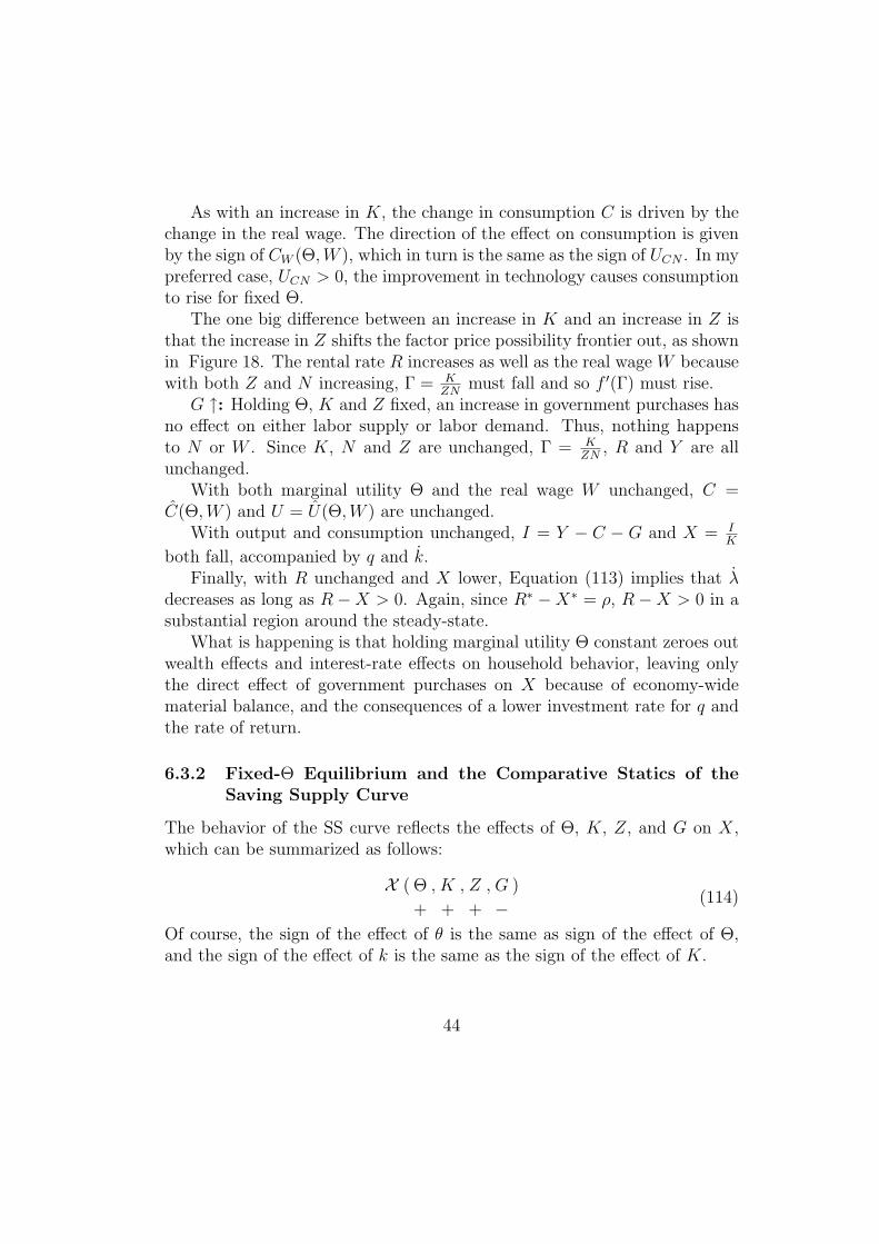
The behavior of the SS curve reflects the effects of Θ, K, Z, and G on X,which can be summarized as follows:

X ( Θ

+

, K

+

, Z

+

, G

−)

(114)

Of course, the sign of the effect of θ is the same as sign of the effect of Θ,and the sign of the effect of k is the same as the sign of the effect of K.

44

Figure 19 shows the Saving Supply (SS) Curve. The positive effect of θon X guarantees that the Saving Supply Curve slopes up. Going up alongthe SS curve, in addition to the increase in the three monotonically relatedvariables X, q and k shown by the increase in X on the graph, it is useful tothink of N , R, Y and I going up as one goes up the curve, while W , Γ andU are lower at higher points on the SS curve.

An increase in the (log) capital stock k shifts the SS curve to the right.At the point on the new SS curve directly to the right of a point on the oldcurve, not only X, q and k, but also N , W , Γ, Y , I and λ (and probably C)are higher, while R and U are lower.

An improvement in technology Z also shifts the SS curve to the right.At the point on the new SS curve directly to the right of a point on the oldcurve, not only X, q and k, but also N , W , R, Y , I and λ (and probably C)are higher, while Γ and U are lower.

An increase in government purchases G shifts the SS curve to the left. Atthe point on the new SS curve directly to the right of the point on the oldcurve, λ is lower in addition to X, q and k being lower.

6.3.3 Fixed-Investment-Rate Equilibrium

Where Fixed-Θ equilibrium picks out the point on the new SS curve directlyto the right of the relevant point on the old SS curve when K, Z or G change,Fixed-X equilibrium picks out the point on the new SS curve directly belowor above the relevant point on the old SS curve.

Table 3 details the comparative statics for Fixed-X equilibrium. The rowfor q and k is easy since both are monotonically increasing functions of X byitself. Also, Equation (112), λ = θ + q(X), implies that holding X constant,λ must move in the same direction as θ. Since an increase in X holding K, Zand G constant turns out to increase θ as well, such an increase in X raisesthe required value of λ.

I will discuss the rest of the comparative statics results in Table 3 columnby column.

45

Table 3: Fixed-Investment-Rate Comparative Statics

X K Z G

λ + − − +N + ? ? +W − + + −Γ − + − −R + − + +Y + + + +C − + + −U − + + −I + + 0 0θ + − − +

q, k + 0 0 0

λ ? + − −The Contemporaneous Preferences and Technology Diagram is the key to

analyzing Fixed-X equilibrium.X ↑: The effects of increasing X in Fixed-X equilibrium must be quali-

tatively the same as the effects of increasing Θ in Fixed-Θ equilibrium, sinceboth cases correspond to movements up along the SS curve, holding K, Zand G fixed. Still, it is useful to see how these results show up in the Contem-poraneous Preferences and Technology Diagram as a way of building moreintuition for the use of the diagram.

As shown in Figure 20 an increase in X causes a parallel downwardshift in the Contemporaneous Material Balance curve. Because the indif-ference curve slope W (C,N) is increasing in C, at the point directly belowthe original tangency, the Contemporaneous Material Balance curve slopeW d(K, N,Z) is greater than the slope W (C, N) of the indifference curvethrough that point (not shown), implying that the new tangency is furtherup the new Contemporaneous Material Balance curve, at a higher level of N .The slope W at the new tangency will be lower than at the original tangency.With K and Z unchanged, Γ = K

ZNwill be lower and R higher than before.

The increase in N also guarantees that Y increases. The fall in KZN

raisesthe rental rate R, in accordance with the factor price possibility frontier, andwith X fixed, Equation (97) implies that λ moves opposite to the rental rateR.

46

I = XK rises because K is unchanged. Felicity U at the new tangencyfalls because the opportunity set is worse. Since both U and W are lower atthe new tangency, Θ = Θ(U,W ) will be higher.

Finally, to see what happens to C in going to the new tangency, considerthe point on the new Contemporaneous Material Balance curve directly tothe right of the original tangency, where C is the same, but N is higher. IfW0 is the slope at the original tangency, W (C, N) > W0 > W d(K, N,Z) atthis point, since the indifference curve slop is increasing in N , while the slopeof the new Contemporaneous Material Balance curve at a higher value of Nis lower than the slope of the original Contemporaneous Material Balancecurve at the original value of N . Therefore, the new tangency is lower downon the new Contemporaneous Material Balance curve than the point thathas the original level of consumption C.

G ↑: Since in increase in G also causes a parallel downward shift in theContemporaneous Material Balance curve, the comparative statics effects ofG conditional on X are identical to the effects of an increase in X, exceptfor the obvious lack of effect of G on q, k and I, given X. Note that the con-frontation of higher government purchases with a Contemporaneous MaterialBalance curve that does not allow G to simply crowd out investment as inthe Fixed-Θ comparative statics yields more intuitive effects of governmentpurchases.

K ↑: As shown in Figure 21, an increase in K shifts the Contempora-neous Material Balance curve up (as long as R − X > 0) and increases itsslope at a given level of labor N because FKN > 0. Also, the concavity ofthe Contemporaneous Material Balance curve guarantees that it has a higherslope at the point on the new curve with the original level of consumptionC.

Because the slope of indifference curves is increasing in both N and C,the point on the new Contemporaneous Material Balance curve directly tothe left of the old tangency point has a flatter indifference curve and a steeperContemporaneous Material Balance curve than the original tangency. Mov-ing up along the Contemporaneous Material Balance curve unambiguouslysteepens the slope of the relevant indifference curve at each point, while flat-tening the slope of the Contemporaneous Material Balance curve. Therefore,the new tangency will be at a point with higher consumption C than the oldtangency. Equation (92) then implies that Y must be higher at the newtangency, since Y = C + I + G and both C and I = XK are higher.

47

Because the new Contemporaneous Material Balance curve is concaveand is steeper than the original Contemporaneous Material Balance curvefor given N , the point on the new Contemporaneous Material Balance curveon the same Engel curve as the original tangency must have W d(K,N, Z) >W (C,N) = W0. Therefore, the new tangency must have a higher real wageW than the original tangency. According to the Factor-Price PossibilityFrontier, the higher value of W must correspond to a higher Γ = K

ZNand a

lower R. Conditional on X, the lower value of R must correspond to a highervalue of λ. Since U and W are both higher, Θ = Θ(U,W ) must be lower atthe new tangency. Felicity U is clearly higher at the new tangency, since thecontemporaneous opportunity set has improved.

The change in labor N in moving to the new tangency is ambiguous, sinceat the point directly above the old tangency, both the ContemporaneousMaterial Balance curve and the relevant indifference curve are steeper thanbefore. If the Contemporaneous Material Balance curve is tilted up moreat that point, then the new tangency will be at a higher N . If the relevantindifference curve is tilted up more at that point, then the new tangencywill be at a lower N . A quasilinear utility function of the form U(C, N) =C − v(N) will have indifference curves directly above with exactly the sameslope; so it is clear that for some utility functions, the new tangency can beat a higher N . Similarly, a quasilinear utility function of the form u(C)−N ,with a strongly concave u(C) will make the indifference curves directly abovehave a much higher slope; so it is clear that for some utility functions, thenew tangency can be at a lower N .

Z ↑: On the Contemporaneous Preferences and Technology Diagram anincrease in Z looks quite similar to an increase in K. The ContemporaneousMaterial Balance curve shifts up and becomes steeper at a given N , butwithout needing to assume that R − X > 0 for the upward shift. Unlikewhen K increases, I does not increase, but C increases since the point tothe left original tangency has a demand wage greater than the supply wage.Y = C + I + G increases because C increases. W increases because thedemand wage is greater than the supply wage at the intersection of theoriginal Engel curve and the new Contemporaneous Material Balance curve.U increases since the opportunity set is greater. Θ is lower because both Uand W are higher. The movement in labor is ambiguous, as it was for anincrease in K.

Although the change in N is ambiguous, since output is an increasing

48

function of K and ZN , and output Y has increased, ZN must be higher.With K unchanged, the higher value of ZN pushes the effective capital/laborratio Γ = K

ZNdown and the rental rate R up. Given X, the increase in R

pushes λ down. These three effects are opposite to the effects of an increasein K.

6.4 II-SS and Contemporaneous General Equilibrium

Equilibrium between investment demand and saving supply is the fulcrumof Contemporaneous General Equilibrium. The major new complication inContemporaneous General Equilibrium is that the investment rate X andthe marginal utility of consumption Θ are endogenous.15

Table 4 gives the signs of the effects of λ, k, Z and G on the key variables.The complications due to the endogeneity of (log) marginal utility θ and theinvestment rate X in Contemporaneous General Equilibrium are detailedbelow. As before, some of the signs noted depend on R−X > 0, which willhold in a substantial region around the steady state.

15While the capital stock k never jumps and the marginal value of capital λ can jumponly when new information arrives, even a fully foreseen change in Z or G can cause θ tojump by shifting the SS curve. Since the real interest rate is

< = ρ− θ,

the (ex ante) real interest rate would be infinite at that point (that is, there would beconversion ratio different from 1 for real funds before and after the point at which Z orG changed in a foreseen way). This kind of a spike in the real interest rate is a reflectionof the fact that < is not itself determined in Contemporaneous General Equilibrium, buthas to do with the rate of change of Contemporaneous General Equilibrium variable θ.

49

Table 4: Contemporaneous General EquilibriumComparative Statics

λ k Z G

N + ? ? +W − + + −Γ − + − −R + − + +Y + + + +C − ? ? −U − ? ? −θ + − − +I + + + −

x, q, k + + + −λ ? + ? −

6.4.1 λ ↑: Shifting Out the II Curve

As shown in Figure 22, an increase in the marginal value of capital λ shiftsthe II curve out, moving the equilibrium to a higher point on the SS curve.Marginal utility θ, the investment rate X, Tobin’s q and k are all higher.Since K, Z and G are being held fixed, in terms of Table 2, only the increasein Θ is operative. Therefore the signs in the column for the effects of λ inTable 4 are identical to those in the column for Θ in Table 2. However, anincrease in λ causes a less-than-one-for-one increase in θ.

6.4.2 Shifts of the SS curve

Figure 23 shows an outward shift of the SS curve. This outward shift in theSS curve could come from an increase in K, and increase in Z, or a decreasein G. Depending on the slope of the II curve, the new intersection could beanywhere on the striped segment of the new SS curve. In other words, forall of the shifts of the SS curve—by K, Z, or G, Contemporaneous GeneralEquilibrium effects will be between the effects when X is fixed and the effectswhen θ is fixed. This is obvious when linearizing or log- linearizing. Lemma2 gives the same result without using linearization.

50

Lemma 2 If a variable moves in an unambiguous direction when movingup along the SS curve, and if a shift in the SS curve by K, Z or G has aconsistent effect on the variable when comparing between Fixed-Θ equilibriumand in Fixed-X equilibrium, then the effect of the shift in the SS curve onthe variable in Contemporaneous General Equilibrium is the same as thatconsistent effect. If the effect in one Fixed equilibrium is zero, then the effectof the shift in the SS curve will be in the same direction as the effect in theother Fixed equilibrium.

Proof: The move to the new intersection of II and SS can be decomposed intoeither the move to the new Fixed-Θ equilibrium plus a movement along theSS curve, or decomposed into a move to the new Fixed-X equilibrium plus amovement along the SS curve in the opposite direction. If the variable movesthe same direction in both Fixed Θ equilibrium and Fixed-X equilibrium, theeffect of the move along the SS curve must be the same as initial shift toa new SS curve in one of these two cases. If the effect on the variable iszero in either Fixed-Θ or Fixed-X equilibrium, this yields an unambiguousprediction for the Contemporaneous General Equilibrium effect, which mustbe consistent with the direction for the other Fixed equilibrium, since the otherFixed equilibrium is further along the SS curve in the same direction beyondthe new intersection of II and SS.

The one Contemporaneous General Equilibrium variable Lemma 2 doesnot cover is λ, where the effect of a movement along the SS curve is ambigu-ous.

The converse to Lemma 2—which I will state less formally—is also useful:unless the movement of a variable depends on the degree of investment ad-justment costs even in the Fixed equilibria, if the direction a variable movesin Fixed- Θ equilibrium is opposite to the direction it moves in Fixed-Xequilibrium, it must be genuinely ambiguous in Contemporaneous GeneralEquilibrium. The reason is that by varying the degree of the investmentadjustment cost, the slope of the II curve can be varied to make Contem-poraneous General Equilibrium effects arbitrarily close to Fixed-Θ effects orFixed-X effects. Also, for the same reason, unless the movement of a vari-able depends on the degree of investment adjustment costs even in the Fixedequilibria, the structure of Contemporaneous General Equilibrium cannoteliminate a genuine ambiguity present in one of the Fixed equilibria.

51

The only variable in which the degree of investment adjustment costsmatters for the direction of an effect in Fixed-Θ or Fixed-X equilibrium isλ. Thus, Lemma 2 and its converse provide the entries in Table 4 for everyrow but the row for λ.

For λ, in the case of an increase in K or G, we can use Equation (113) tosay that when the investment rate X and the rental rate R move in oppositedirections, λ must move in the same direction as X. The effect of Z on λis genuinely ambiguous, since a very small investment adjustment cost willmake λ go opposite to R and therefore fall when Z increases in Contempora-neous General Equilibrium. To show that λ can go up in ContemporaneousGeneral Equilibrium with an increase in Z, fix a particular strength of theinvestment adjustment costs, thereby determining a given relationship be-tween the movement of X and Θ when the shift in the SS curve moves theintersection of II and SS along the II curve. Then making the productionfunction f more and more linear will make any movement in R = f ′

(K

ZN

)

very small, so that the positive effect of X on λ will dominate.Finally, note that the additional assumption UCN > 0 could eliminate

the ambiguity of the effect of k and Z on consumption in Contemporane-ous General Equilibrium: both would then have a positive effect, since theywould have a positive effect in both Fixed-Θ equilibrium and Fixed-X equi-librium. The effect of k and Z on consumption in Contemporaneous GeneralEquilibrium is also unambiguously positive in the additively separable caseUCN = 0.

6.5 An Important Special Case: The Basic Real Busi-ness Cycle Model

Let me call the model of Prescott (1986), with a more general felicity functionU and a more general production function f , the Basic Real Business CycleModel. Then the Basic Real Business Cycle Model is the limiting specialcase of the QRBC Model when there is no investment adjustment costs:J(X) = X − δ. Since with J ′(X) ≡ 1,

Θ = ΛJ ′(X) = Λ,

the II curve θ = λ + ln J ′(X) is flat, and Contemporaneous General Equilib-rium for the Basic Real Business Cycle Model is identical to Fixed-Θ equi-

52

librium. Moreover, the absence of investment adjustment costs simplifies thedetermination of λ, since with J ′(X) ≡ 1, since Equation (97)reduces to

λ = ρ + δ −R.

Since Θ = Λ,

ρ−< = θ = λ = ρ + δ −R,

implying

r = R− δ

in the absence of investment adjustment costs.The additional structure on λ insures that λ always moves opposite to the

rental rate in the Basic Real Business Cycle Model. Thus, the one changeto Table 2 as a description of the Contemporaneous General Equilibriumcomparative statics for the Basic Real Business Cycle model is that in theabsence of investment adjustment costs, an increase in Θ = Λ unambiguouslylowers λ.

6.6 Immediate Applications of Contemporaneous Gen-eral Equilibrium

In addition to its role as a building block for determining dynamic generalequilibrium, Contemporaneous General Equilibrium also serves as a usefulapproximation for the effects of shocks to Z or G that are so short-lived thatthey have relatively little effect on either k or λ. In other words, the last twocolumns of Table 4 show the effects of very short-lived shocks to Z and G.

Another immediate application of contemporaneous general equilibriumis that it shows the effects of anticipated, but sudden movements in Z orG. The log marginal value of capital λ can only jump when there is newinformation. Thus, when sudden movements in Z or G are foreseen, λ cannotjump at that moment. The capital stock K never jumps. As a result, thechanges at that moment of sudden, anticipated change are driven by thechanges in Z or G holding λ and K fixed.

Thus, treating λ as if it were exogenous is very useful in cases where λwill not move very much. It is also useful in situations where the direction

53

λ jumps or evolves is known. What about cases such as a permanent im-provement in technology, in which λ can jump either up or down on impact,depending on parameters? Then Contemporaneous General Equilibrium isnot as immediately helpful. For this particular case, knowledge about thebehavior X on impact, together with the structure of Fixed-X equilibrium,can help in the analysis. More generally, any time one has knowledge of thebehavior of a variable, structural analysis treating that variable as if it wereexogenous can sometimes be useful.

7 Dynamic General Equilibrium

My ultimate objective is to characterize the impulse responses to technol-ogy and government purchase shocks. These impulse responses come out ofDynamic General Equilibrium.

7.1 The Phase Diagram

The Contemporaneous General Equilibrium comparative statics for k andλ indicate the dynamics that show up directly on the phase diagram. Thedynamics of k and λ are central to dynamic general equilibrium because kcan never jump, while λ can jump only when new information arrives. In theanalysis of the impulse response to a single bundle of new information arrivingat “time zero” this means that the impulse response for λ can only jump attime zero, at the moment when the new information arrives. Beyond thatmoment, both intertemporal variables k and λ act as slowly moving anchorsto the behavior of the model, helping to determine the rest of the key variablesthrough the machinery of Contemporaneous General Equilibrium.

The positive effects of both k and λ on k in Table 4 indicate that thek = 0 locus is downward sloping, with k > 0 above the locus and k < 0below.

The positive effect of k on λ indicates that λ > 0 to the right of the λ = 0locus, while λ < 0 to the left. Because of the ambiguous effect of λ on λ,whether the λ = 0 locus is upward-sloping, downward-sloping, or verticaldepends on parameters.16 With no investment adjustment costs, the Basic

16Totally inelastic labor supply and no investment adjustment costs yields the Ramsey-Cass-Koopmans Model which has a vertical λ = 0 locus.

54

Real Business Cycle Model has a negative effect of λ on λ and therefore anupward-sloping λ = 0 locus.

If the λ = 0 locus were not only downward-sloping, but tilted back somuch that it was flatter than the k = 0 locus, it would make the dynamicstotally unstable. Fortunately, the positive effect of K on λ in the Fixed-Xequilibrium guarantees that the λ = 0 locus is downward sloping, it mustbe more steeply downward sloping than the k = 0 locus where the two lociintersect. The key to seeing this is that k = 0 implies X = δ, so X is fixed asone moves along the k = 0 locus. Increasing k while letting λ fall to stay onthe k = 0 equilibrium makes λ rise in accordance with Fixed-X equilibrium.Therefore the points on the k = 0 locus to the right of the intersection mustbe in the region to the right of the λ = 0 locus, which can only happen if theλ = 0 locus is more steeply downward-sloping, vertical or upward-sloping.

Figure 24 shows the three possible cases for the phase diagram. In eachcase, there is a downward-sloping saddle path that shows the dynamics if Zand G are constant. Since Λ is the marginal value of capital, Λ = VK(K),and the saddle-path gives the relevant value of Λ for the optimal dynamicprogram, the downward-sloping saddle path is a reflection of the concavity ofthe value function, VKK(K) < 0. The concavity of the value function in turnarises from the fact that the social planner’s problem is a concave problemin all of its components.

7.2 Behavior Along the Saddle Path

Table 5 indicates how key variables evolve as the economy moves along thesaddle path. Since λ is fully endogenous in Dynamic General Equilibrium,it makes sense to think of the behavior along the saddle path as governedby the value of the (log) capital stock k inherited from the past at any givenmoment. An increase in k corresponds to moving down along the saddle pathto a higher capital stock, as the economy will do if the initial capital stockis below its steady-state value. If instead the initial capital stock is higherthan the steady-state value, the economy will move up the saddle path onthe other side of the steady state, and all the signs in Table 5 get multipliedby the negative movement of the capital stock, as the capital stock graduallyfalls back to its steady-state value.

55

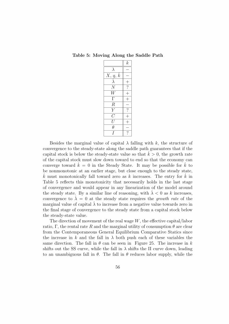
Table 5: Moving Along the Saddle Path

k

λ −X, q, k −

λ +N ?W +Γ +R −Y ?C +U +θ −I ?

Besides the marginal value of capital λ falling with k, the structure ofconvergence to the steady-state along the saddle path guarantees that if thecapital stock is below the steady-state value so that k > 0, the growth rateof the capital stock must slow down toward to end so that the economy canconverge toward k = 0 in the Steady State. It may be possible for k tobe nonmonotonic at an earlier stage, but close enough to the steady state,k must monotonically fall toward zero as k increases. The entry for k inTable 5 reflects this monotonicity that necessarily holds in the last stageof convergence and would appear in any linearization of the model aroundthe steady state. By a similar line of reasoning, with λ < 0 as k increases,convergence to λ = 0 at the steady state requires the growth rate of themarginal value of capital λ to increase from a negative value towards zero inthe final stage of convergence to the steady state from a capital stock belowthe steady-state value.

The direction of movement of the real wage W , the effective capital/laborratio, Γ, the rental rate R and the marginal utility of consumption θ are clearfrom the Contemporaneous General Equilibrium Comparative Statics sincethe increase in k and the fall in λ both push each of these variables thesame direction. The fall in θ can be seen in Figure 25. The increase in kshifts out the SS curve, while the fall in λ shifts the II curve down, leadingto an unambiguous fall in θ. The fall in θ reduces labor supply, while the

56

increase in k raises labor demand, guaranteeing an increase in the real wageW , accompanied by an increase in the effective capital/labor ratio Γ and adecrease in the rental rate R in accordance with the Factor Price PossibilityFrontier.

The signs for consumption C and felicity U are guaranteed by the struc-ture of Fixed-X equilibrium, in view of the gradual decline in the investmentrate X in the last stage of convergence as the economy nears a higher steady-state level of capital. Intuitively, as capital accumulates and the effort towardaccumulating yet more capital abates, the economy has more resources forcurrent felicity. The increase in real wage as the economy goes down thesaddle path then guarantees that the improvement in felicity will come morefrom increased consumption and less from increased leisure than it wouldalong an Engel curve.

What about the real interest rate <? Unlike the other variables, the realinterest is not determined by k, λ, Z and G at a given moment in Contem-poraneous General Equilibrium. But in Dynamic General Equilibrium, thebehavior of < can be seen from

< = ρ− θ.

Since θ declines as the capital stock increases along the Saddle Path,

< > ρ

along the left-hand arm of the Saddle Path where k > 0 while < < ρ onthe right-hand arm of the Saddle Path where k < 0. In either case, the realinterest < must eventually go back towards a value of ρ at the Steady State.

7.3 The Dynamic General Equilibrium Response to aPermanent Increase in Government Purchases

There are two ways to analyze how the two isoclines k = 0 and λ = 0shift when there is a permanent increase in additively separable governmentpurchases, financed by an increase in lump-sum taxes. One way is to lookat the effects of G in Contemporaneous General Equilibrium of on k and λ.The negative effect G on k in Contemporaneous General Equilibrium meansit would require an increase in either k or λ to cancel out the effect of the

57

increase in G on k. Therefore, an increase in G shifts the k = 0 locus outwardand upward. The negative effect of G on λ in Contemporaneous GeneralEquilibrium means that, holding λ fixed, it would require an increase in kto cancel out the effect of the increase in G on λ. Therefore the λ = 0locus shifts to the right. The λ = 0 locus shifts right with an increase in Gregardless of the slope of the λ = 0 locus, since the variations in the slopeof the λ = 0 locus come from the ambiguity in the effect of λ on λ, which Isidestepped by considering how to get back to λ = 0 while holding λ fixed.The other way to analyze how the two isoclines shift is to realize that theintersection of the k = 0 locus and the λ = 0 locus must shift in accordancewith the steady-state effects on k and λ indicated by Table 1: the intersectionmust be at a higher level of both k and λ. Figure 26 shows the two maincases for the dynamic path on the phase diagram. The case of a verticalλ = 0 locus would have an appearance between the appearance of these twocases. In both cases, the (log) marginal value of capital λ must jump up onimpact and then fall gradually as the economy moves down the saddle pathto a new, higher level of capital. The reason the slope of the λ = 0 locusmakes so little difference to the qualitative picture is: (1) the direction inwhich the new steady state shifts is totally unaffected by adjustment costsand (2) the saddle path is always downward sloping.

What about the other key variables? The QRBC model has only one en-dogenous state variable, k. Therefore the response to immediate permanentshocks is composed of an impact effect, a saddle path effect as the capitalstock adjusts to the new value, and a steady-state effect that is the sum ofthe impact effect and the saddle-path effect. Table 6 shows for key variablesthe impact effect, saddle path effect, and steady-state effect of an immediate,permanent increase in additively separable government purchases, financedby an increase in lump-sum taxes. Given the increase in the steady-statecapital stock generated by a permanent increase in G, the saddle-path ef-fects for each variable are those given in Table 5. The steady-state effects forare the same as those given in Table 1.

58

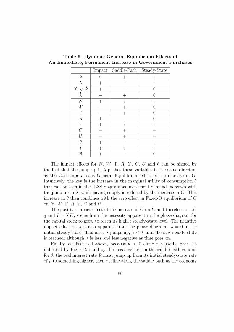
Table 6: Dynamic General Equilibrium Effects ofAn Immediate, Permanent Increase in Government Purchases

Impact Saddle-Path Steady-State

k 0 + +λ + − +

X, q, k + − 0

λ − + 0N + ? +W − + 0Γ − + 0R + − 0Y + ? +C − + −U − + −θ + − +I + ? +< + − 0

The impact effects for N , W , Γ, R, Y , C, U and θ can be signed bythe fact that the jump up in λ pushes these variables in the same directionas the Contemporaneous General Equilibrium effect of the increase in G.Intuitively, the key is the increase in the marginal utility of consumption θthat can be seen in the II-SS diagram as investment demand increases withthe jump up in λ, while saving supply is reduced by the increase in G. Thisincrease in θ then combines with the zero effect in Fixed-Θ equilibrium of Gon N , W , Γ, R, Y , C and U .

The positive impact effect of the increase in G on k, and therefore on X,q and I = XK, stems from the necessity apparent in the phase diagram forthe capital stock to grow to reach its higher steady-state level. The negativeimpact effect on λ is also apparent from the phase diagram. λ = 0 in theinitial steady state, than after λ jumps up, λ < 0 until the new steady-stateis reached, although λ is less and less negative as time goes on.

Finally, as discussed above, because θ < 0 along the saddle path, asindicated by Figure 25 and by the negative sign in the saddle-path columnfor θ, the real interest rate < must jump up from its initial steady-state rateof ρ to something higher, then decline along the saddle path as the economy

59

approaches the new Steady State and return to a value of ρ at the new SteadyState.

7.4 The Dynamic General Equilibrium Response to aPermanent Improvement in Technology

An increase in Z raises k in Contemporaneous General Equilibrium. Thisincrease can be cancelled out by an reduction in either k or λ. Therefore, anincrease in Z causes the k = 0 locus to shift down. The ambiguous effect ofZ on λ in Fixed-X equilibrium indicates that the λ = 0 locus can shift eitherright or left. In accordance with Table 1, the new steady state must be at ahigher capital stock k and a lower marginal value of capital λ. As shown inFigure 27, the key ambiguity is that the marginal value of capital can jumpeither up or down on impact, depending on the slope of the saddle path incomparison with the vector direction of the shift from the old Steady Stateto the New Steady State. (As in Figure 26, the qualitative possibilities arenot much altered when the λ = 0 locus if vertical or downward sloping, sincethe shift of the new steady state is unaffected by adjustment costs.) Thisambiguity in which way λ jumps makes it impossible to sign the impact effectsof an immediate, permanent increase in Z simply by adding or subtractingcolumns of Table 4.

Fortunately, the structure of Dynamic General Equilibrium guaranteesthat since the new steady-state value of capital is higher, k > 0 and λ < 0along the saddle path, which in turn implies that the investment rate k, q andX must jump up on impact.17 Since both Z and X jump up on impact, whileG does nothing and K cannot jump, the structure of Fixed-X equilibriumguarantees that R, Y and I increase on impact, while Γ = K

ZNjumps down.

The impact effects on λ, N , W , C U and θ are ambiguous. Although theinitial jump in θ on impact is ambiguous, by the logic of Figure 25, it mustbe that θ < 0 thereafter as the economy moves down the new saddle pathto the new Steady State at a higher level of capital. Since < = ρ − θ, thisimplies that < > ρ along the saddle path. Therefore, < must jump up onimpact from its original value of ρ.

By particular numerical examples of log-linearized models, I have verified

17If the shock to Z hits an economy that begins out of steady-state, this statement relieson linearization.

60

that the impact effect on λ, N , W , C, U and θ are all genuinely ambiguous,but the details I leave to a future companion paper.1819

labor N goes up or down as the economy goes down the saddle pathas capital’s share α is higher or lower than the elasticity of intertemporalsubstitution s. As for output Y , in the limiting case where U(C,N) =ln(C)−N , output will go up or down with evolution down the saddle pathdepending on whether capital’s share α is greater or less than 1/3.

18In brief, suppose one focuses on the Basic Real Business Cycle model, which is thelimit of the QRBC model as the investment adjustment cost becomes very small (so thatθ = λ), with King-Plosser-Rebelo preferences of the form

U(C, N) =C1−s−1

1− s−1φ(N)

and impatience ρ very close to zero (for convenience, one can look at the limiting equationsas ρ → 0). Then and an elasticity of intertemporal substitution s significantly greater thanone, coupled with a low elasticity of substitution between capital and labor (low enoughthat it barely obeys the restriction σ > α that is equivalent to FNZ > 0), makes the impacteffects on λ, N and θ positive while the impact effects on W , C and U are negative. Onthe other hand, if the production function is Cobb-Douglas, with capital’s share equal to1/3, while the elasticity of intertemporal substitution s is less than 1/3, the impact effectson λ, N and θ are negative, while the impact effect on W , C and U are positive. Thevalue of the labor supply elasticity determined by the shape of φ(N) is not crucial forany of these statements, though there are some restrictions on φ(N) needed to guaranteeconcavity of U(C,N) and the normality of consumption and leisure.

19I have also verified by numerical examples closely related to those of the previousfootnote that the directions of evolution of N , Y and I along the saddle path are am-biguous. With ρ ≈ 0 in the Basic RBC model with King-Plosser-Rebelo preferences anda Cobb-Douglas production function that has capital’s share α = 1/3, moving down thesaddle path will cause labor, output and investment to go down for a high enough elastic-ity of intertemporal substitution s (and in the case of output, a high enough labor supplyelasticity); while a low enough value of s will ensure that N , Y and I go up as the economymoves down the saddle path.

61

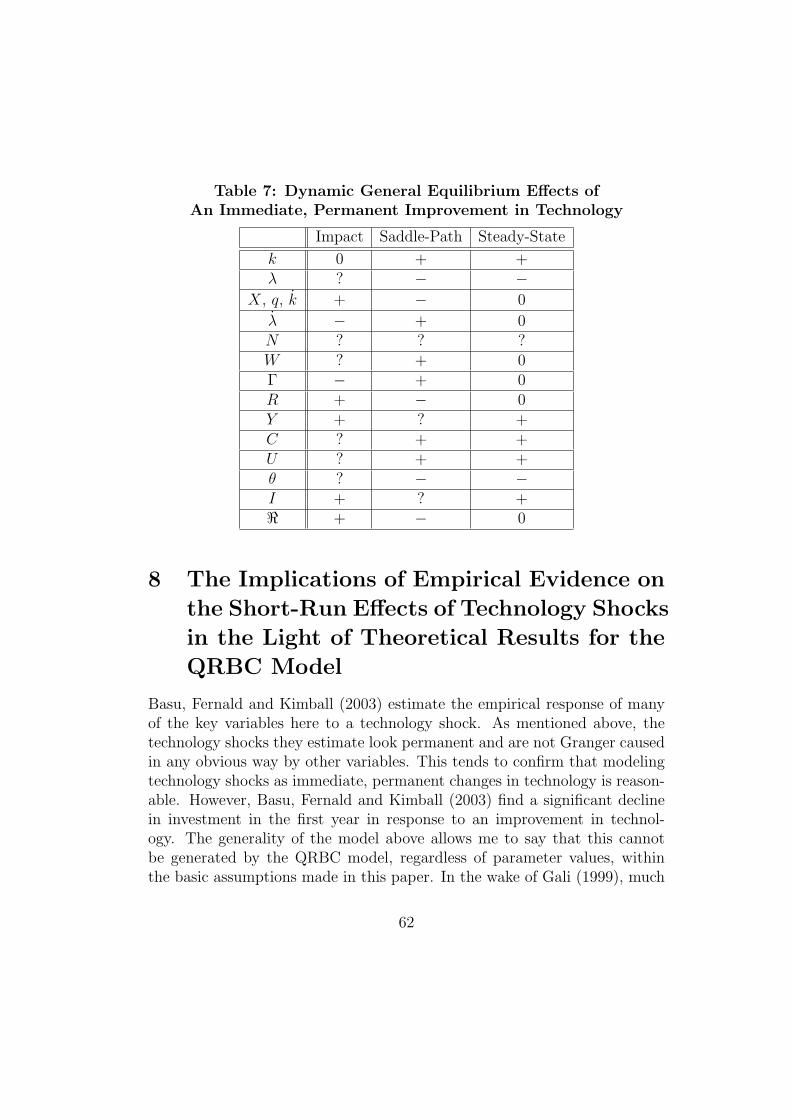
Table 7: Dynamic General Equilibrium Effects ofAn Immediate, Permanent Improvement in Technology

Impact Saddle-Path Steady-State

k 0 + +λ ? − −

X, q, k + − 0

λ − + 0N ? ? ?W ? + 0Γ − + 0R + − 0Y + ? +C ? + +U ? + +θ ? − −I + ? +< + − 0

8 The Implications of Empirical Evidence on

the Short-Run Effects of Technology Shocks

in the Light of Theoretical Results for the

QRBC Model

Basu, Fernald and Kimball (2003) estimate the empirical response of manyof the key variables here to a technology shock. As mentioned above, thetechnology shocks they estimate look permanent and are not Granger causedin any obvious way by other variables. This tends to confirm that modelingtechnology shocks as immediate, permanent changes in technology is reason-able. However, Basu, Fernald and Kimball (2003) find a significant declinein investment in the first year in response to an improvement in technol-ogy. The generality of the model above allows me to say that this cannotbe generated by the QRBC model, regardless of parameter values, withinthe basic assumptions made in this paper. In the wake of Gali (1999), much

62

of the attention garnered by the evidence for contractionary technologicalimprovements has focused on the estimated negative response of employ-ment to an improvement in technology found by both Gali (1999) and Basu,Fernald and Kimball (2003), by very different methods. But the decline ininvestment found by Basu, Fernald and Kimball (2003) is more decisive inrejecting a real business cycle model explanation of the effects of technologyshocks than the decline in employment, since it a straightforward matter tofind parameter values for which the QRBC model, or other closely relatedmodels imply a negative response of employment to a technological improve-ment. By contrast, it is quite difficult (though presumably not impossible,given enough cleverness) to generate a decline in investment in response toa technological improvement as the sensible response of a social planner whoultimately wants to get to a higher capital stock. A decline in output Y orthe real interest rate would also be relatively decisive in rejecting a modellike the QRBC model. Although these results are not statistically significant,Basu, Fernald and Kimball do find a decline in output in the first year of atechnological improvement, and a long-lived decline in the real interest rateafter a technological improvement begins.

What about the possibility that, despite point estimates to the contraryby Basu, Fernald and Kimball (2003), a technology shock involves a phase-inperiod in which true total-factor productivity will be even higher tomorrowthan it is today as the new technology is more fully implemented? It is easyto see from the phase diagram that an anticipated future improvement intechnology, which has an immediate effect only through the marginal valueof capital λ can cause a contraction in employment, output and investment ifλ jumps down enough in response to the news. The relevant case is associatedwith a wealth effect that is large in comparison to the interest rate effect,as can be seen most easily by looking again at Equation (29), which withθ = ln(Θ), is

θ(t) = θ(∞) +∫ ∞

t[<(τ)− ρ]dτ.

If technology improves now and will improve more in the future, it is like acombination of an immediate permanent technology shock of the size of theimmediate improvement in technology with an anticipated future technologyshock that goes further.

In analyzing a phase-in period for technology as an explanation for a

63

decline in investment caused by a technological improvement within theframework of the QRBC model, the robustness of Contemporaneous Gen-eral Equilbrium structures to the dynamic path of variables is useful. Theperspective of Fixed-X equilibrium as described in Table 3 indicates that ifthe investment rate falls on impact in response to a technological improve-ment, consumption and the real wage must go up. (Just subtract the Xcolumn from the Z column.) Here the robustness to the details about thefuture path of technology comes from the fact that, given the current valuesof K, Z and G, the current investment rate X embodies the key informationabout the future.

Alternatively, take the observation that employment falls in response toa technological improvement. In the QRBC model, labor demand dependsonly on the current values of K and Z. An increase in Z shifts labor demandout. Given slow movement in K so that we can neglect its effects, if N fallsat the same time labor demand shifts out, the real wage W must increase inthe QRBC model.

The increase in the real wage W coupled with a decrease in N thenimplies an increase in consumption. Along a given Engel curve, a decreasein N is associated with an increase in C. A higher real wage pushes therepresentative household above the original Engel curve, in the direction ofhigher C.

Thus, in the QRBC model, an increase in current Z associated witheither a fall in the investment rate I/K or a fall in employment N , must beassociated with an increase in consumption and the real wage, regardless ofwhat technology is going to do beyond that moment in time. This result isbased primarily on the assumptions that consumption and leisure are normaland that technology and labor are supermodular in the production function:FNZ > 0.

Is the entire exercise here self-destructive? Is it an analysis of the QRBCmodel only to show that it cannot be true? My answer is no. Models build onone another. In particular, a Neoclassical sticky-price model needs a solid realbusiness model as its backbone, describing the nature of the full employmentequilibrium that the economy tends toward as prices adjust. Kimball (1995)implicitly uses a variant of the QRBC model in just this fashion.

64

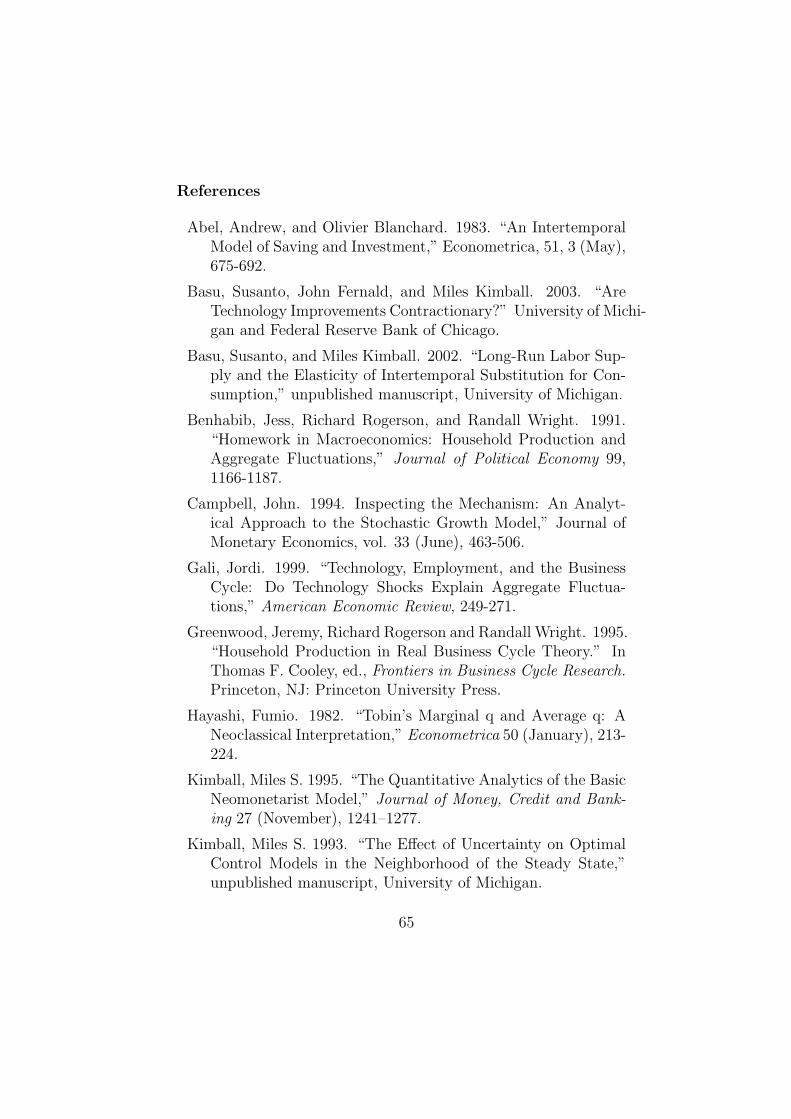
References

Abel, Andrew, and Olivier Blanchard. 1983. “An IntertemporalModel of Saving and Investment,” Econometrica, 51, 3 (May),675-692.

Basu, Susanto, John Fernald, and Miles Kimball. 2003. “AreTechnology Improvements Contractionary?” University of Michi-gan and Federal Reserve Bank of Chicago.

Basu, Susanto, and Miles Kimball. 2002. “Long-Run Labor Sup-ply and the Elasticity of Intertemporal Substitution for Con-sumption,” unpublished manuscript, University of Michigan.

Benhabib, Jess, Richard Rogerson, and Randall Wright. 1991.“Homework in Macroeconomics: Household Production andAggregate Fluctuations,” Journal of Political Economy 99,1166-1187.

Campbell, John. 1994. Inspecting the Mechanism: An Analyt-ical Approach to the Stochastic Growth Model,” Journal ofMonetary Economics, vol. 33 (June), 463-506.

Gali, Jordi. 1999. “Technology, Employment, and the BusinessCycle: Do Technology Shocks Explain Aggregate Fluctua-tions,” American Economic Review, 249-271.

Greenwood, Jeremy, Richard Rogerson and Randall Wright. 1995.“Household Production in Real Business Cycle Theory.” InThomas F. Cooley, ed., Frontiers in Business Cycle Research.Princeton, NJ: Princeton University Press.

Hayashi, Fumio. 1982. “Tobin’s Marginal q and Average q: ANeoclassical Interpretation,” Econometrica 50 (January), 213-224.

Kimball, Miles S. 1995. “The Quantitative Analytics of the BasicNeomonetarist Model,” Journal of Money, Credit and Bank-ing 27 (November), 1241–1277.

Kimball, Miles S. 1993. “The Effect of Uncertainty on OptimalControl Models in the Neighborhood of the Steady State,”unpublished manuscript, University of Michigan.

65

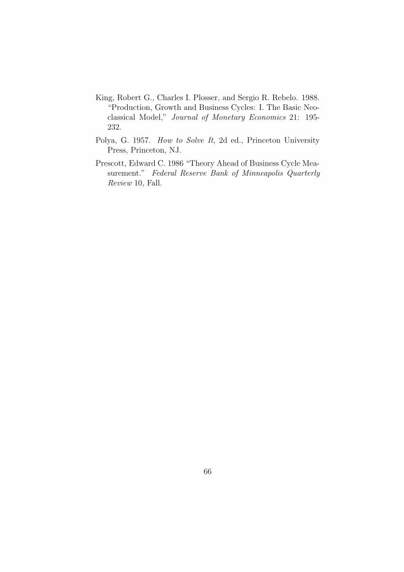
King, Robert G., Charles I. Plosser, and Sergio R. Rebelo. 1988.“Production, Growth and Business Cycles: I. The Basic Neo-classical Model,” Journal of Monetary Economics 21: 195-232.

Polya, G. 1957. How to Solve It, 2d ed., Princeton UniversityPress, Princeton, NJ.

Prescott, Edward C. 1986 “Theory Ahead of Business Cycle Mea-surement.” Federal Reserve Bank of Minneapolis QuarterlyReview 10, Fall.

66

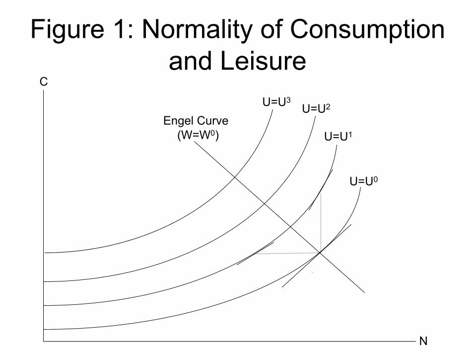
C

N

Engel Curve(W=W0)

U=U0

U=U1

U=U2U=U3

Figure 1: Normality of Consumption and Leisure

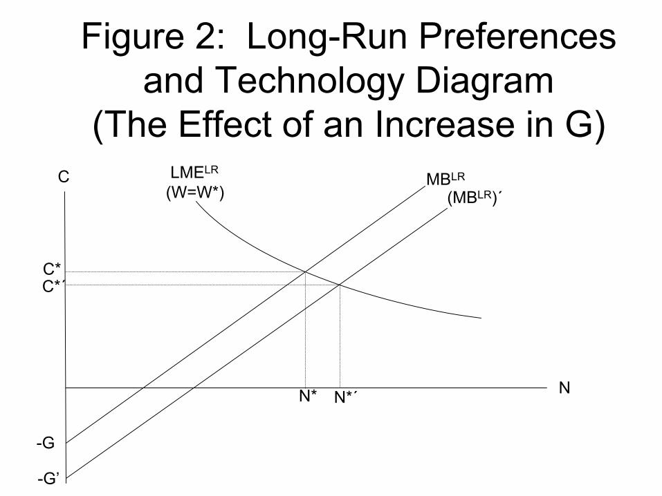
Figure 2: Long-Run Preferences and Technology Diagram

(The Effect of an Increase in G)C

N

MBLR

(MBLR)´LMELR

(W=W*)

-G

-G’

N* N*΄

C*C*´

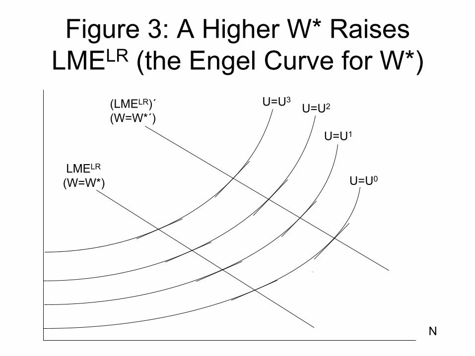
Figure 3: A Higher W* Raises LMELR (the Engel Curve for W*)

N

U=U0

U=U1

U=U2U=U3

LMELR

(W=W*)

(LMELR)´(W=W*´)

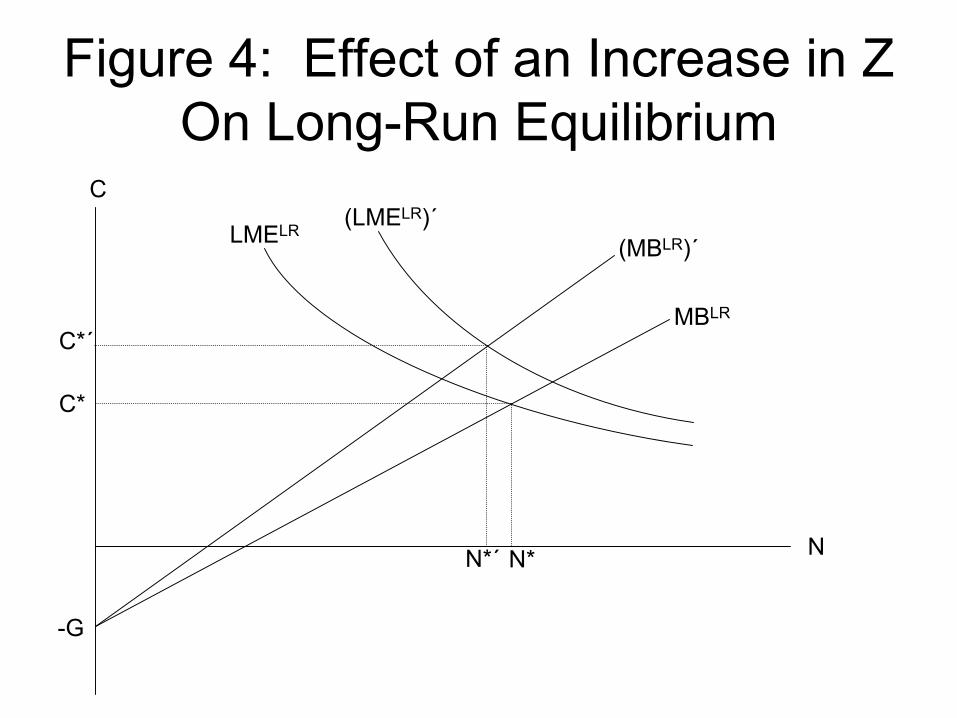
Figure 4: Effect of an Increase in Z On Long-Run Equilibrium

C

N

MBLR

(MBLR)´LMELR

-G

N*N*΄

C*

C*´

(LMELR)´

Figure 5: Illustration of Lemma 1

β

F (β,…)

F (ξ2 ,β,…)

F (ξ0 ,β,…)

F (ξ1 ,β,…)

F

ˆ

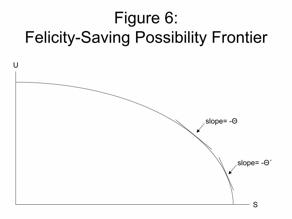
Figure 6:Felicity-Saving Possibility Frontier

S

U

slope= -Θ

slope= -Θ´

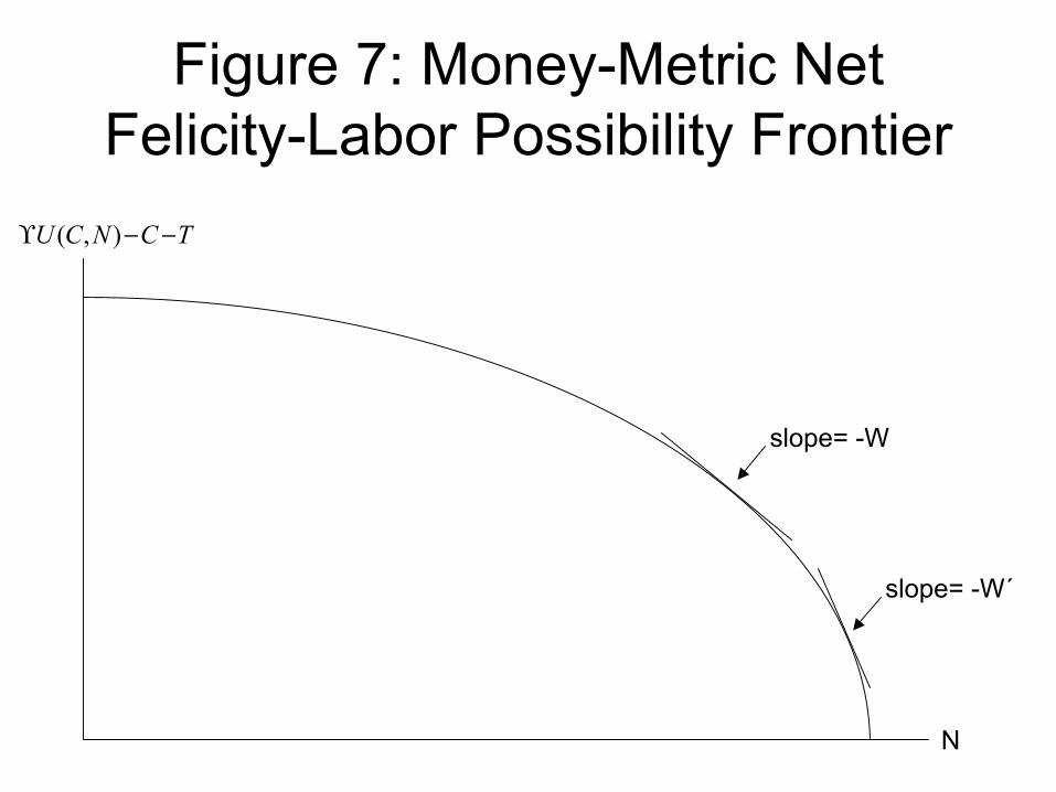
Figure 7: Money-Metric Net Felicity-Labor Possibility Frontier

N

slope= -W

slope= -W´

( , )U C N C Tϒ − −

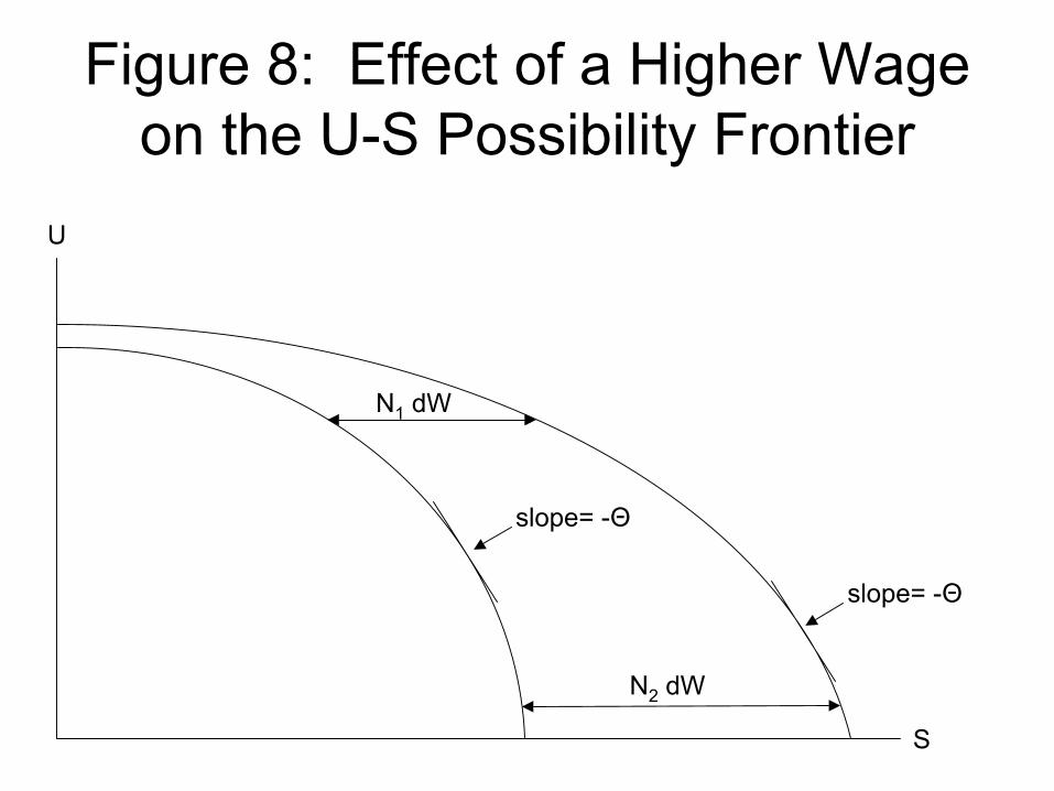
Figure 8: Effect of a Higher Wage on the U-S Possibility Frontier

S

U

slope= -Θ

slope= -Θ

N2 dW

N1 dW

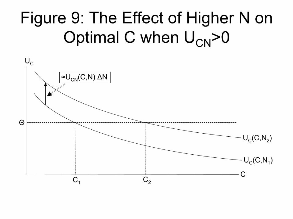
Figure 9: The Effect of Higher N on Optimal C when UCN>0

C

UC

Θ

UC(C,N2)

UC(C,N1)

C1 C2

≈UCN(C,N) ∆N

Figure 10: The Factor Price Possibility Frontier

W

R

FPPF(Z)

slope= -N/K

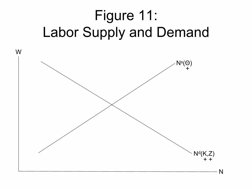
Figure 11: Labor Supply and Demand

W

N

Nd(K,Z)

Ns(Θ)+

+ +

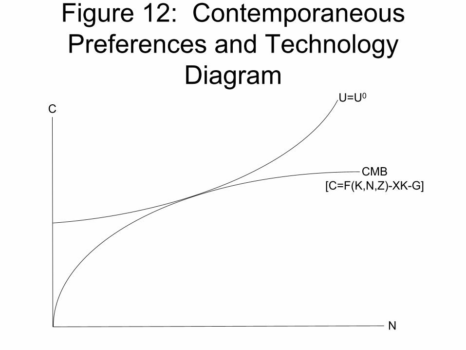
Figure 12: Contemporaneous Preferences and Technology

DiagramU=U0

C

N

CMB[C=F(K,N,Z)-XK-G]

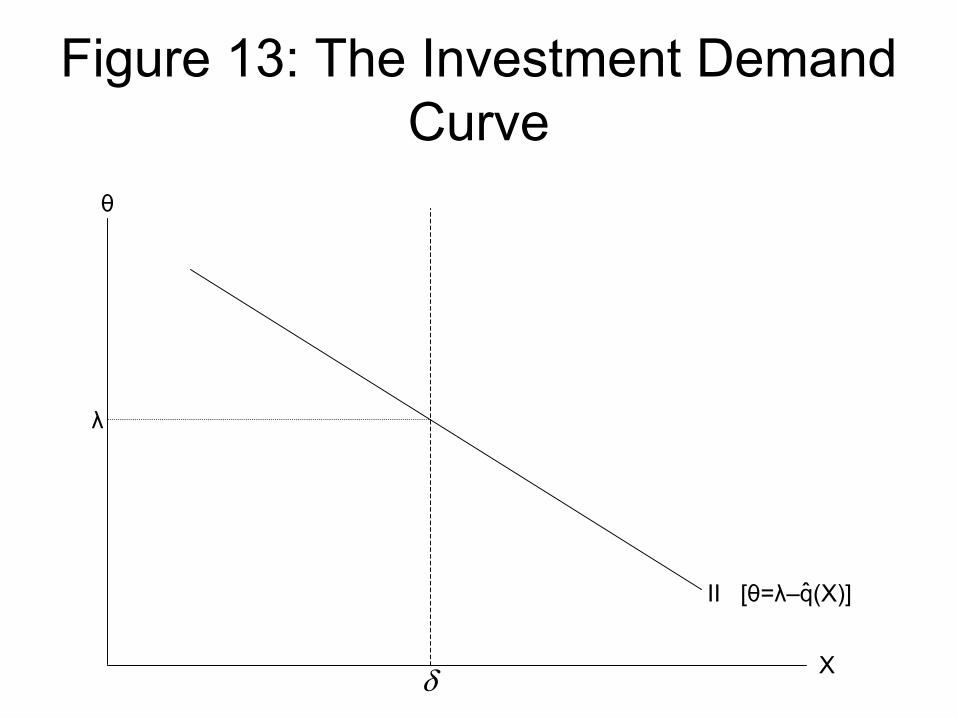
Figure 13: The Investment Demand Curve

θ

Xδ

II [θ=λ–q(X)]ˆ

λ

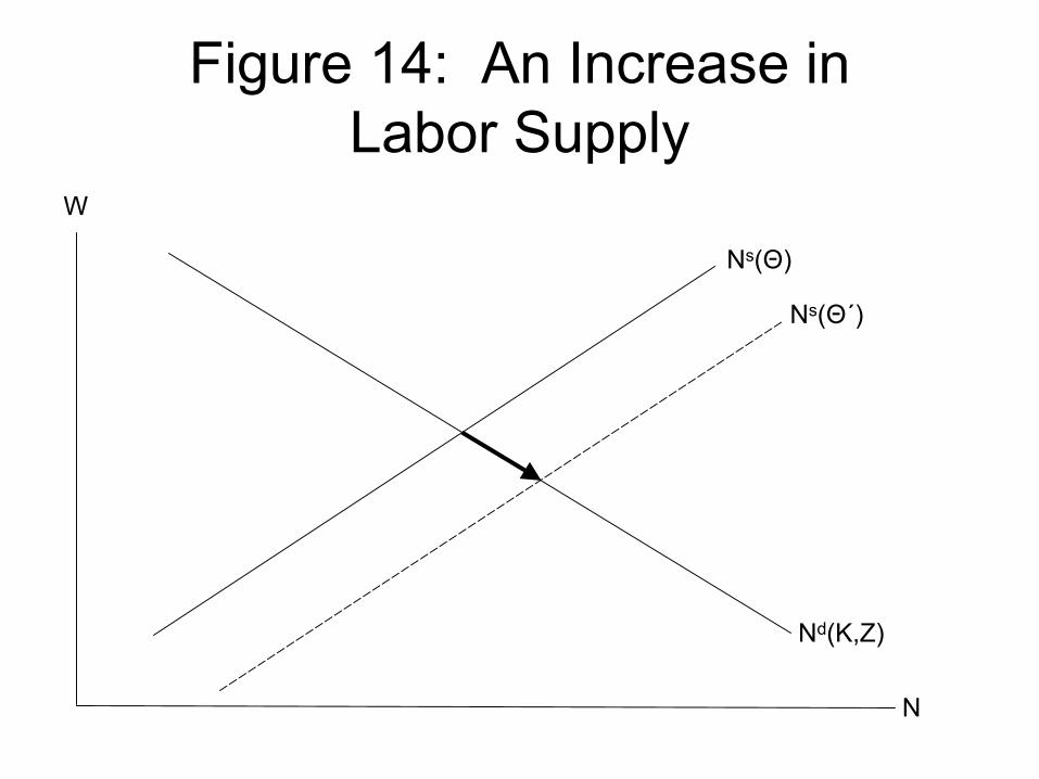
Figure 14: An Increase in Labor Supply

N

Nd(K,Z)

Ns(Θ)

Ns(Θ´)

W

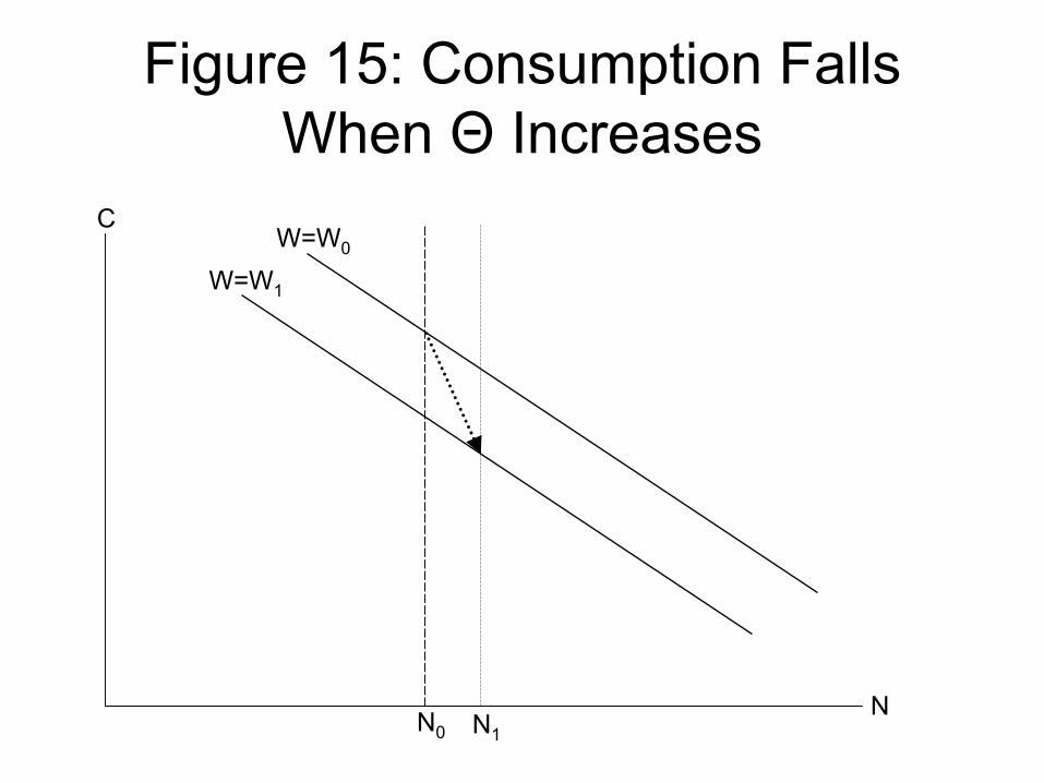
Figure 15: Consumption Falls When Θ Increases

C

N

W=W0

W=W1

N0 N1

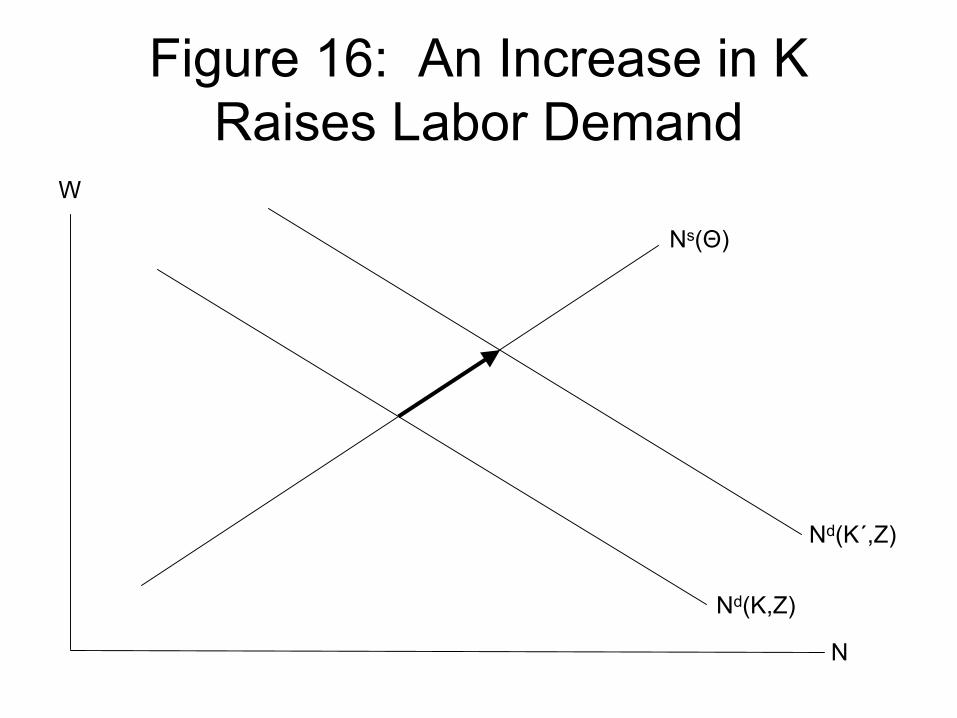
Figure 16: An Increase in K Raises Labor Demand

N

Nd(K,Z)

Ns(Θ)

W

Nd(K΄,Z)

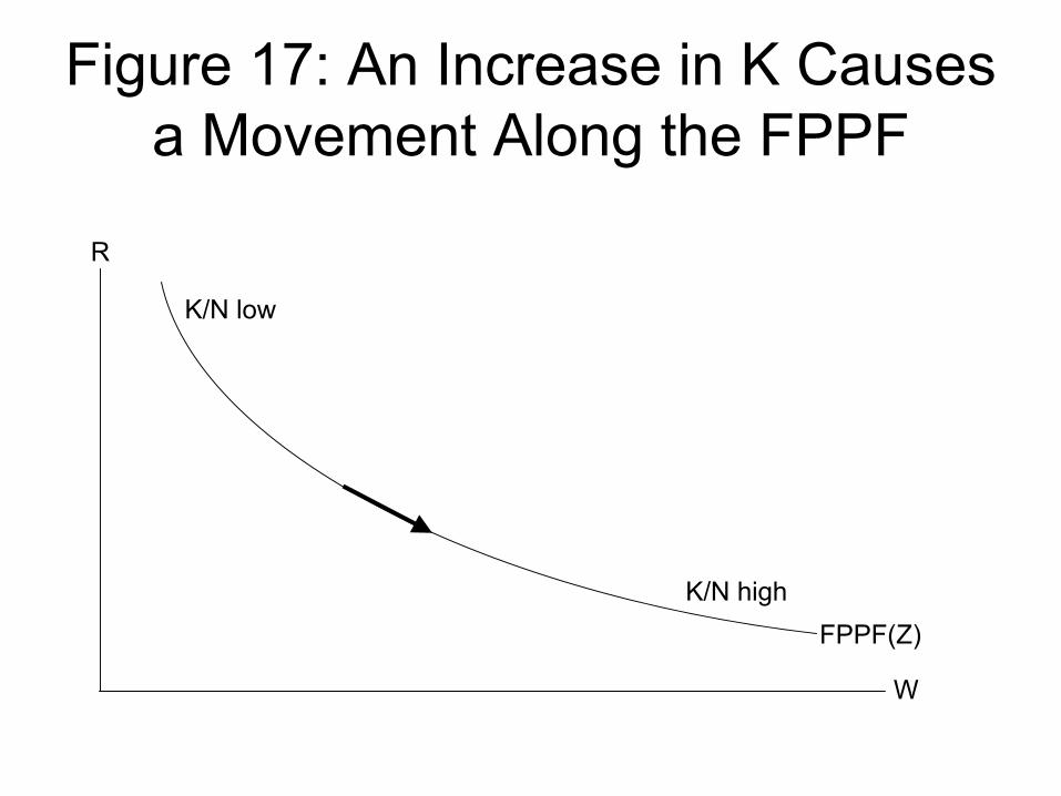
Figure 17: An Increase in K Causes a Movement Along the FPPF

W

R

FPPF(Z)K/N high

K/N low

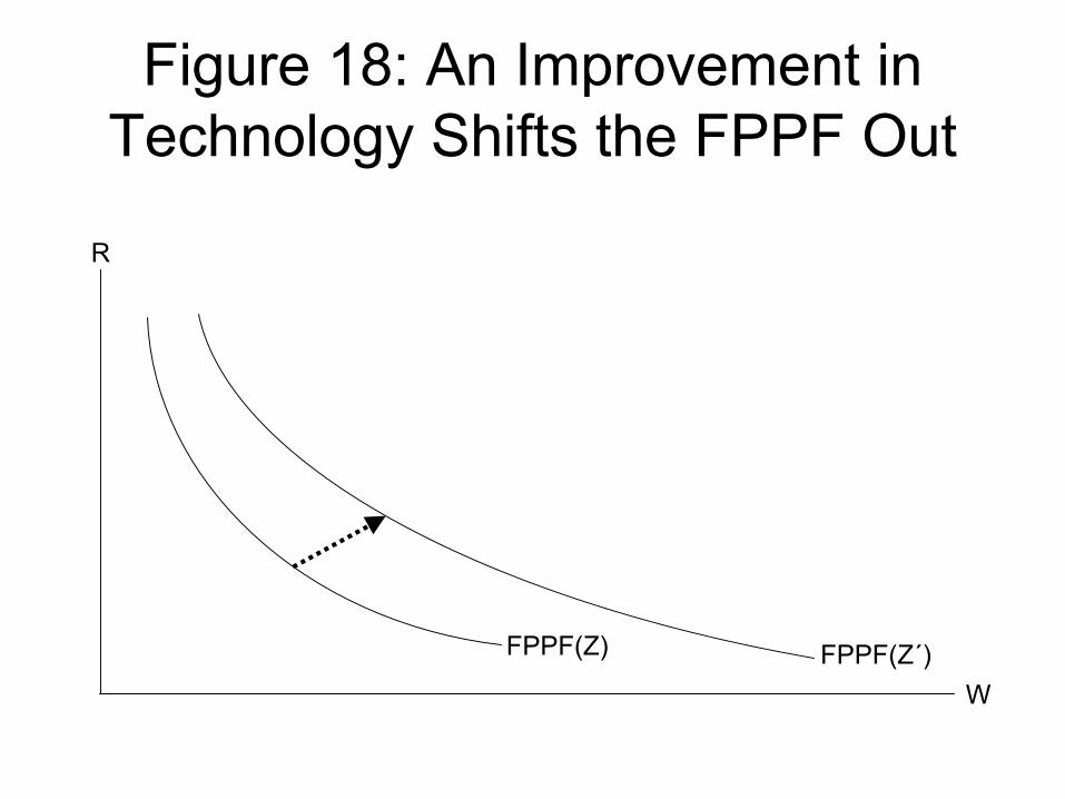
Figure 18: An Improvement in Technology Shifts the FPPF Out

W

R

FPPF(Z) FPPF(Z΄)

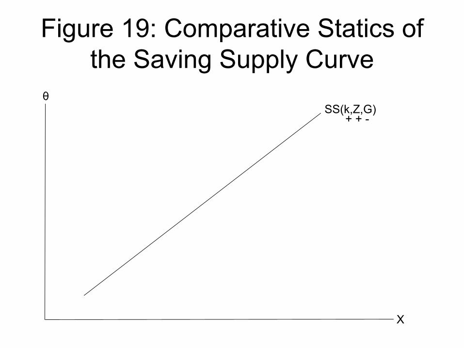
Figure 19: Comparative Statics of the Saving Supply Curve

X

θSS(k,Z,G)

+ + -

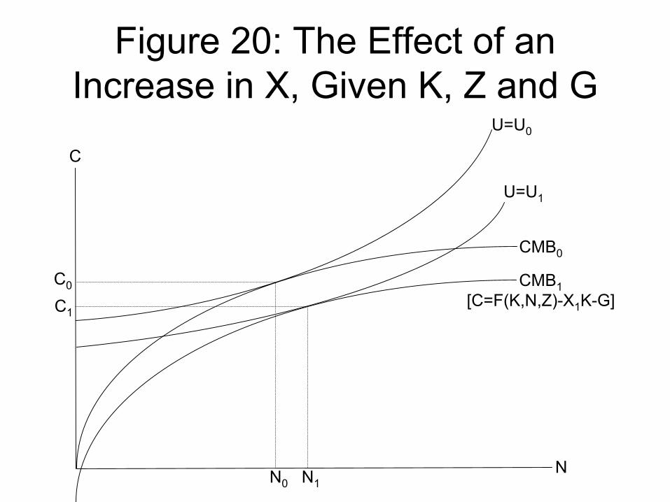
Figure 20: The Effect of an Increase in X, Given K, Z and G

C

CMB0

CMB1[C=F(K,N,Z)-X1K-G]

N

U=U0

U=U1

N0 N1

C1

C0

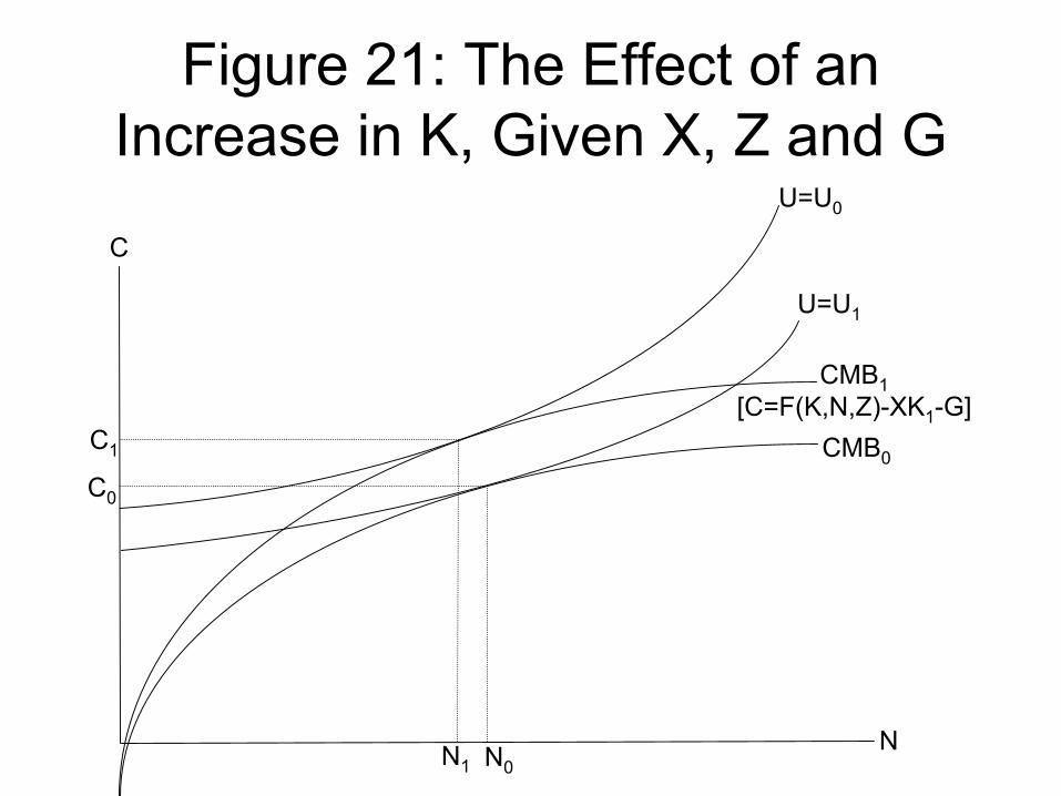
Figure 21: The Effect of an Increase in K, Given X, Z and G

C

CMB0

CMB1[C=F(K,N,Z)-XK1-G]

N

U=U0

U=U1

N0N1

C1

C0

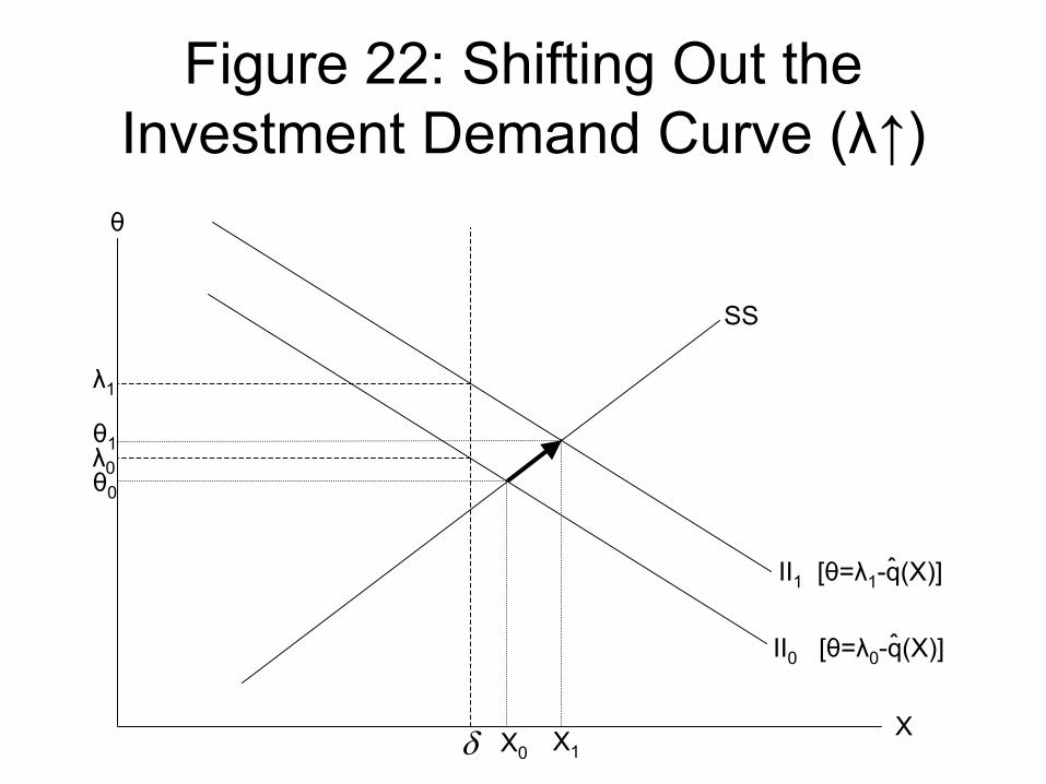
Figure 22: Shifting Out the Investment Demand Curve (λ↑)θ

Xδ

II0 [θ=λ0-q(X)]ˆ

λ0

II1 [θ=λ1-q(X)]ˆ

λ1

SS

θ0

θ1

X0 X1

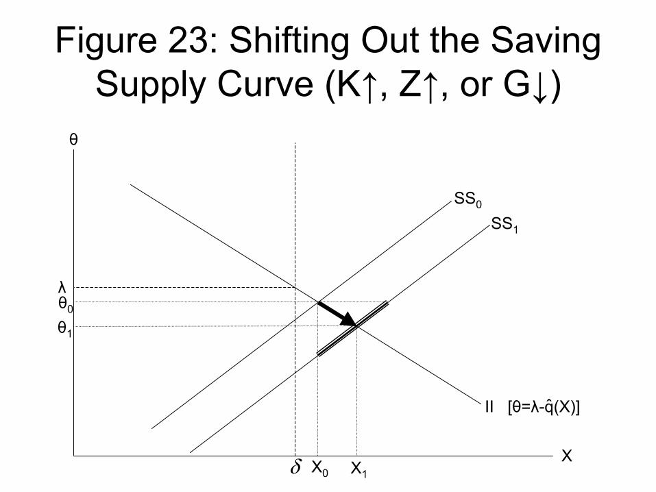
Figure 23: Shifting Out the Saving Supply Curve (K↑, Z↑, or G↓)

θ

Xδ

II [θ=λ-q(X)]ˆ

λ

SS0

θ0

θ1

SS1

X0 X1

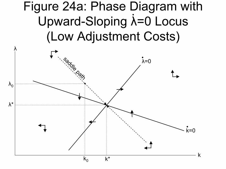
Figure 24a: Phase Diagram with Upward-Sloping λ=0 Locus

(Low Adjustment Costs)

•

k

λ

λ=0•

k=0•

saddle path

k0 k*

λ0

λ*

•

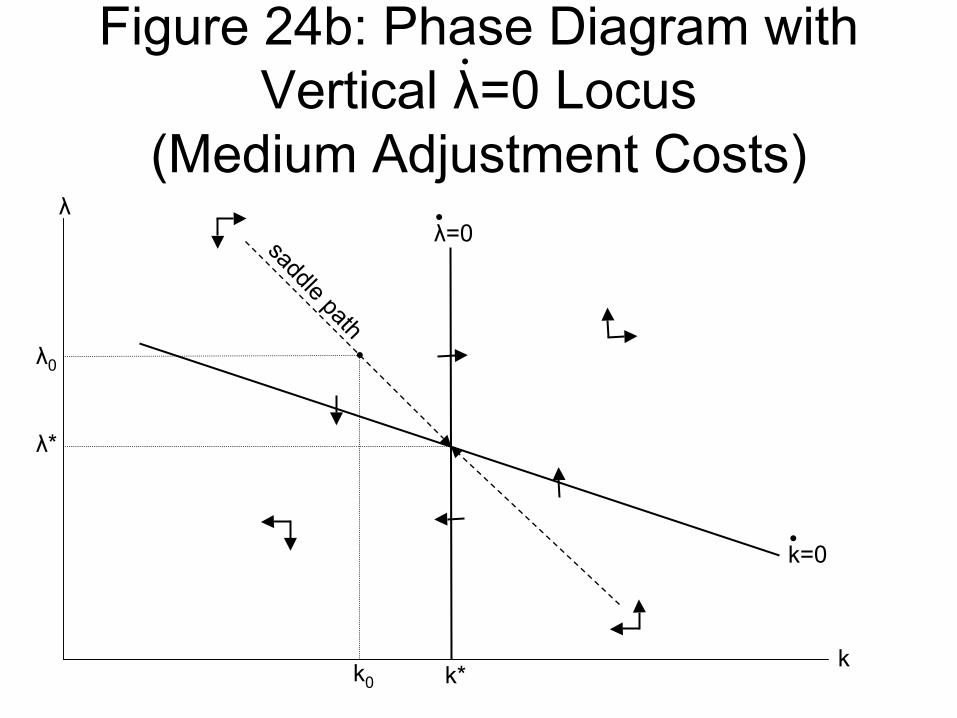
Figure 24b: Phase Diagram with Vertical λ=0 Locus

(Medium Adjustment Costs)

•

k

λλ=0•

k=0•

saddle path

k0 k*

λ0

λ*

•

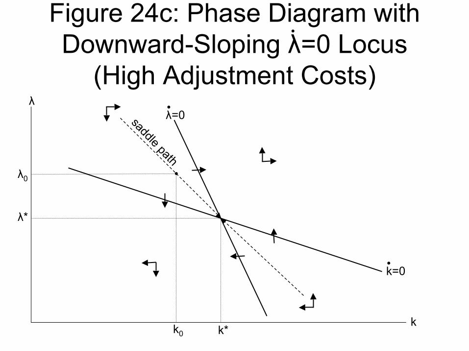
Figure 24c: Phase Diagram with Downward-Sloping λ=0 Locus

(High Adjustment Costs)

•

k

λλ=0•

k=0•

saddle path

k0 k*

λ0

λ*

•

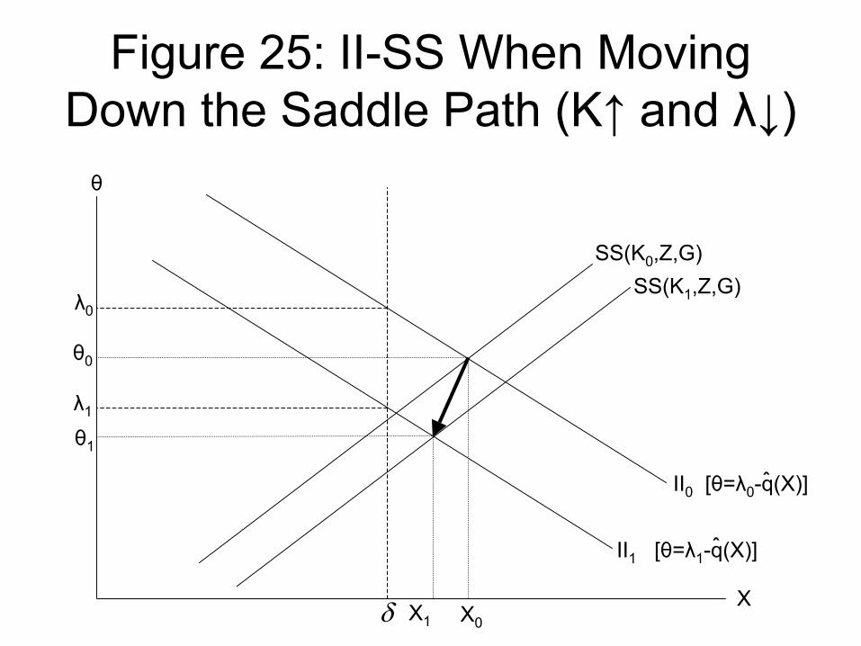
Figure 25: II-SS When Moving Down the Saddle Path (K↑ and λ↓)

θ

Xδ

II1 [θ=λ1-q(X)]ˆ

λ1

SS(K0,Z,G)

θ0

θ1

SS(K1,Z,G)

X1 X0

II0 [θ=λ0-q(X)]ˆ

λ0

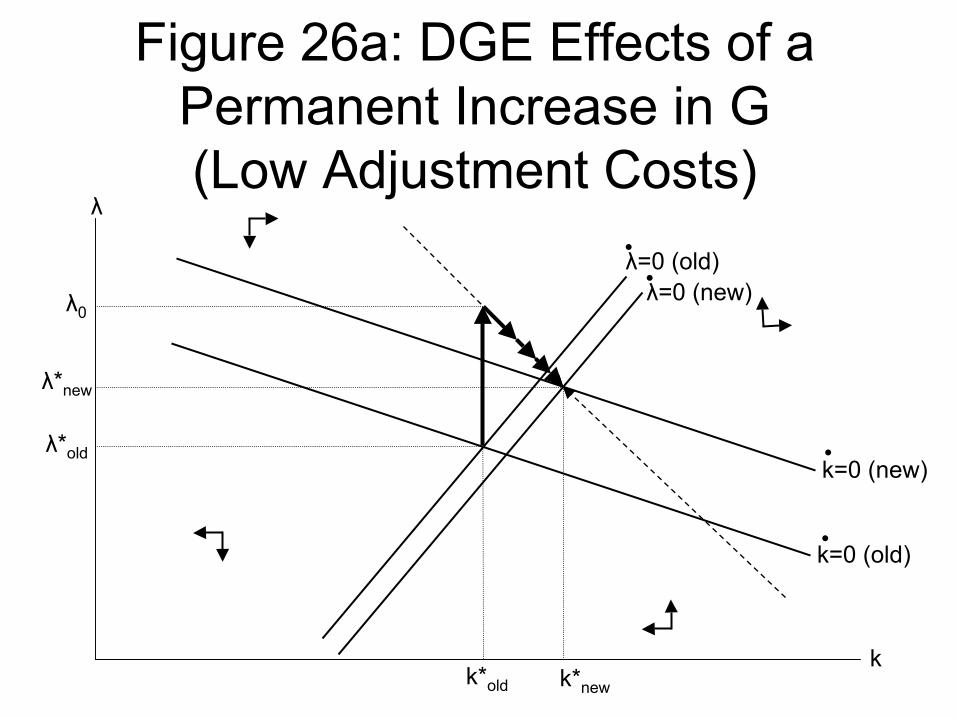
k

λ

λ=0 (old)•

k=0 (old)•

k*newk*old

λ*new

λ*old

Figure 26a: DGE Effects of a Permanent Increase in G(Low Adjustment Costs)

k=0 (new)•

λ=0 (new)•λ0

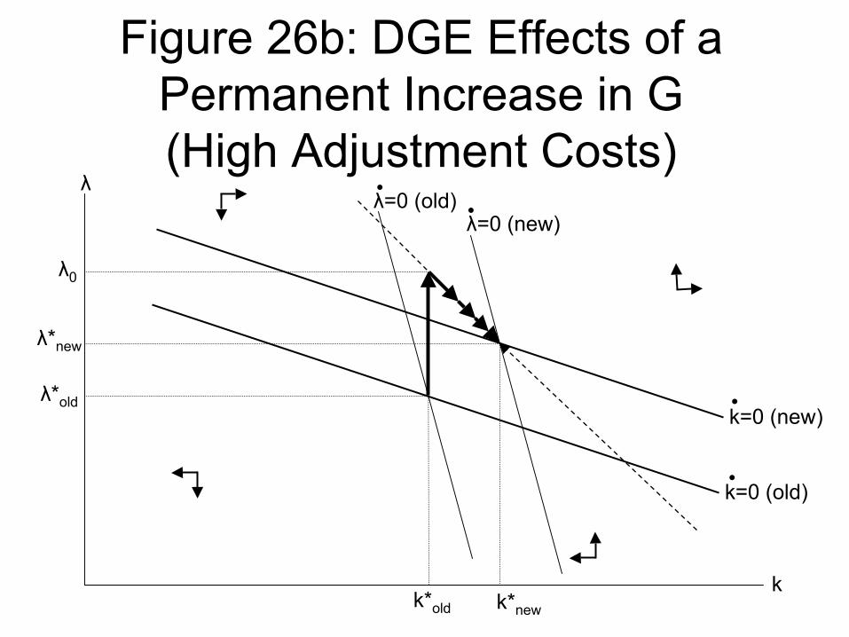
k

λλ=0 (old)•

k=0 (old)•

k*newk*old

λ*new

λ*old

Figure 26b: DGE Effects of a Permanent Increase in G(High Adjustment Costs)

k=0 (new)•

λ=0 (new)•

λ0

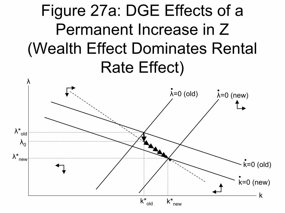
k

λ

λ=0 (old)•

k=0 (old)•

k*newk*old

λ*new

λ*old

Figure 27a: DGE Effects of a Permanent Increase in Z

(Wealth Effect Dominates Rental Rate Effect)

k=0 (new)•

λ=0 (new)•

λ0

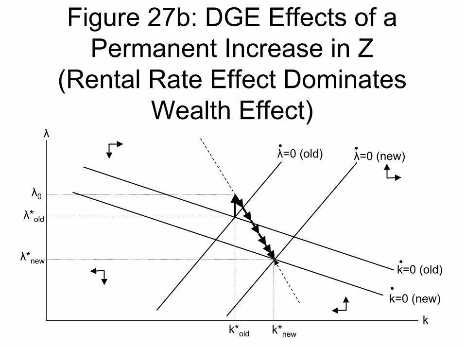
k

λ

λ=0 (old)•

k=0 (old)•

k*newk*old

λ*new

λ*old

Figure 27b: DGE Effects of a Permanent Increase in Z

(Rental Rate Effect Dominates Wealth Effect)

k=0 (new)•

λ=0 (new)•

λ0

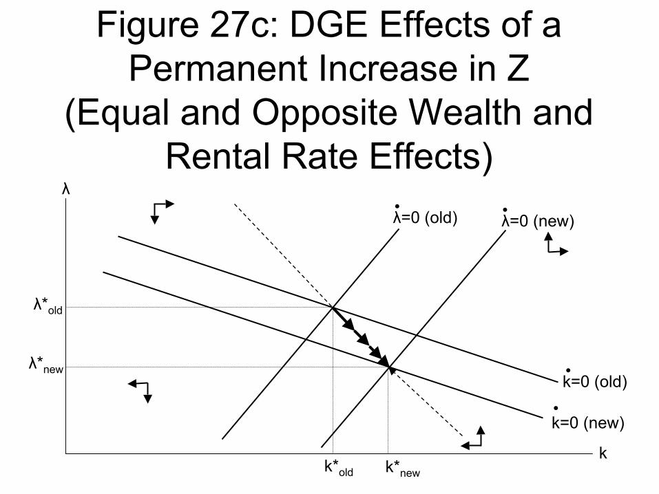
k

λ

λ=0 (old)•

k=0 (old)•

k*newk*old

λ*new

λ*old

Figure 27c: DGE Effects of a Permanent Increase in Z

(Equal and Opposite Wealth and Rental Rate Effects)

k=0 (new)•

λ=0 (new)•