Embed Size (px)
Citation preview

PyroSim Example Guide
2012

PyroSim Example Guide


Table of Contents
iv
Table of Contents PyroSim Example Guide ......................................................................................................... ii Table of Contents .................................................................................................................. iv Table of Figures ................................................................................................................... vii Chapter 1. Before Starting ......................................................................................................1
Install PyroSim.............................................................................................................................. 1 Units ............................................................................................................................................. 1 Manipulating the 3D Image ......................................................................................................... 1 FDS Concepts and Nomenclature ................................................................................................ 1
Chapter 2. Burner Fire ............................................................................................................3 Create the Mesh .......................................................................................................................... 3 Create the Burner Surface ........................................................................................................... 4 Create the Burner Vent ................................................................................................................ 5 Create the Top Vent ..................................................................................................................... 6 Add a Thermocouple .................................................................................................................... 6 Add a Temperature Slice Plane .................................................................................................... 6 Orbit the Model for a Better View ............................................................................................... 7 Save the Model ............................................................................................................................ 7 Run the Simulation ....................................................................................................................... 7 View Smoke in 3D ........................................................................................................................ 9 View Temperature Slice Plane ..................................................................................................... 9 View Temperature Measurements ............................................................................................ 10
Chapter 3. Air Movement ..................................................................................................... 11 Create Mesh ............................................................................................................................... 11 Create the Supply Surface .......................................................................................................... 12 Create Vents ............................................................................................................................... 13 Create Slice Records ................................................................................................................... 15 Specify Simulation Properties .................................................................................................... 15 Save the Model .......................................................................................................................... 16 Run the Simulation ..................................................................................................................... 16 View Particles ............................................................................................................................. 16 View Slice Data ........................................................................................................................... 17
Chapter 4. Smoke Layer Height and Heat Flow Through a Door ............................................. 18 Create the Burner Surface ......................................................................................................... 18 Create the Burner Vent .............................................................................................................. 19 Create the Open Side Vent ........................................................................................................ 20 Create the Mesh ........................................................................................................................ 21 Add the Wall .............................................................................................................................. 21 Add the Door .............................................................................................................................. 22 Orbit the Model for a Better View ............................................................................................. 22 Add a Layer Zoning Device ......................................................................................................... 23 Add a Flow Measuring Device .................................................................................................... 23 Set the Simulation Time ............................................................................................................. 24 Save the model .......................................................................................................................... 24 Run the Simulation ..................................................................................................................... 24 View Smoke in 3D ...................................................................................................................... 25

Table of Contents
v
View Time History Data.............................................................................................................. 26 Chapter 5. Room Fire ........................................................................................................... 27
Import Reaction and Material Data ........................................................................................... 27 Save the Model .......................................................................................................................... 28 Create the Mesh ........................................................................................................................ 28 Specify Combustion Parameters ................................................................................................ 29 Create Surfaces .......................................................................................................................... 30 Create Furniture (Obstructions) ................................................................................................. 32 Walls ........................................................................................................................................... 36 Create Door (Hole in Wall) ......................................................................................................... 37 Use Vents to Define the Burner Fire and Floor .......................................................................... 38 Add an Open Boundary .............................................................................................................. 39 Hang a Picture to the Wall ......................................................................................................... 39 Create Thermocouple Records .................................................................................................. 40 Create Slice Records for 3D Results Plotting .............................................................................. 40 Create Boundary Records .......................................................................................................... 40 Specify Simulation Properties .................................................................................................... 41 The Model is Completed ............................................................................................................ 41 Run the Analysis ......................................................................................................................... 41 View the Results ......................................................................................................................... 42
Chapter 6. Switchgear Fire Example ...................................................................................... 44 Computational Mesh ................................................................................................................. 46 Material Properties .................................................................................................................... 48 Save the Model .......................................................................................................................... 50 Surface Properties ...................................................................................................................... 50 Model Geometry ........................................................................................................................ 52 Post-Processing Controls ........................................................................................................... 68 Simulation Parameters............................................................................................................... 70 Run the Analysis ......................................................................................................................... 70 View the Results ......................................................................................................................... 71
Chapter 7. Single Room Evacuation ...................................................................................... 75 Enable FDS+EVAC ....................................................................................................................... 75 Create Mesh ............................................................................................................................... 75 Create an Exit ............................................................................................................................. 76 Add Occupants ........................................................................................................................... 77 Specify Simulation Properties .................................................................................................... 78 Save the Model .......................................................................................................................... 78 Run the Analysis ......................................................................................................................... 78 View the Results ......................................................................................................................... 78 Using Pathfinder to Solve the Same Problem ............................................................................ 79 Define the Room ........................................................................................................................ 80 Create an Exit ............................................................................................................................. 80 Add Occupants ........................................................................................................................... 80 Specify Simulation Properties .................................................................................................... 81 Save the Model .......................................................................................................................... 81 Run the Analysis ......................................................................................................................... 81 View the Results ......................................................................................................................... 81
Chapter 8. Example Problems Provided with FDS 5 ............................................................... 83

Table of Contents
vi
Ethanol Pan Fire ......................................................................................................................... 83 Box Burn Away ........................................................................................................................... 85 Insulated Steel Column .............................................................................................................. 86 Water Cooling ............................................................................................................................ 87 Evacuation .................................................................................................................................. 88
References ........................................................................................................................... 90

Table of Figures
vii
Table of Figures Figure 2.1. Burner fire in this example .......................................................................................................... 3
Figure 2.2. Creating the mesh ....................................................................................................................... 4
Figure 2.3. Inserting a new burner surface ................................................................................................... 5
Figure 2.4. Defining parameters for the burner surface ............................................................................... 5
Figure 2.5. Creating the burner vent............................................................................................................. 6
Figure 2.6. The Burner Fire model ................................................................................................................ 7
Figure 2.7. The simulation dialog during the analysis ................................................................................... 8
Figure 2.8. The initial Smokeview display ..................................................................................................... 9
Figure 2.9. 3D smoke in the model ............................................................................................................... 9
Figure 2.10. Temperature contours on the slice plane ............................................................................... 10
Figure 2.11. Temperature time history plot ............................................................................................... 10
Figure 3.1. 3D visualization of air flow in this example .............................................................................. 11
Figure 3.2. Creating the mesh ..................................................................................................................... 12
Figure 3.3. Naming the new supply surface ................................................................................................ 12
Figure 3.4. Creating a new supply surface .................................................................................................. 13
Figure 3.5. Creating the new blow vent ...................................................................................................... 14
Figure 3.6. The resulting view ..................................................................................................................... 15
Figure 3.7. Slice record data ....................................................................................................................... 15
Figure 3.8. Defining the simulation parameters ......................................................................................... 16
Figure 3.9. View in Smokeview ................................................................................................................... 17
Figure 3.10. View in Smokeview of velocity contours ................................................................................ 17
Figure 4.1. Smoke in the model .................................................................................................................. 18
Figure 4.2. Creating a new burner surface.................................................................................................. 19
Figure 4.3. Defining parameters for the burner surface ............................................................................. 19
Figure 4.4. Creating the burner vent........................................................................................................... 20
Figure 4.5. Creating the mesh ..................................................................................................................... 21
Figure 4.6. Creating the wall ....................................................................................................................... 22
Figure 4.7. The model after rotating. The burner is shown in red and the top vent in blue. .................... 23
Figure 4.8. The simulation dialog during the analysis. ................................................................................ 24
Figure 4.9. The initial Smokeview display. .................................................................................................. 25
Figure 4.10. 3D smoke in the model. .......................................................................................................... 25
Figure 4.11. Time history plot of heat flow through the door. ................................................................... 26
Figure 4.12. Time history plot of smoke layer height. ................................................................................ 26
Figure 5.1. Room fire in this example ......................................................................................................... 27
Figure 5.2. Copy the reaction from the library ........................................................................................... 28
Figure 5.3. Creating the mesh ..................................................................................................................... 29
Figure 5.4. The POLYURETHANE reaction parameters. .............................................................................. 30
Figure 5.5. Creating the floor surface. ........................................................................................................ 31

Table of Figures
viii
Figure 5.6. Input for the couch base ........................................................................................................... 33
Figure 5.7. The room after the couch is added ........................................................................................... 35
Figure 5.8. The resulting room display........................................................................................................ 36
Figure 5.9. Drawing the wall ....................................................................................................................... 37
Figure 5.10. The model after adding the door ............................................................................................ 38
Figure 5.11. Completed model ................................................................................................................... 41
Figure 5.12. Heat release rate isosurface and temperature contours ....................................................... 42
Figure 5.13. Heat release rate ..................................................................................................................... 43
Figure 6.1. Pictorial representation of the switchgear room complex ....................................................... 44
Figure 6.2. Completed model ..................................................................................................................... 45
Figure 6.3. Input to create the mesh .......................................................................................................... 47
Figure 6.4. Display of the meshes ............................................................................................................... 48
Figure 6.5. Copy the material data from the library to the model ............................................................. 49
Figure 6.6. Thermo-plastic properties ........................................................................................................ 50
Figure 6.7. Composition of the concrete surface........................................................................................ 51
Figure 6.8. The concrete surface ................................................................................................................. 51
Figure 6.9. Input for the wall dividing the two rooms ................................................................................ 54
Figure 6.10. Display of the dividing wall ..................................................................................................... 54
Figure 6.11. The contol logic that opens the dividing door ........................................................................ 56
Figure 6.12. Sketch of the lower left cabinet .............................................................................................. 58
Figure 6.13. Making a copy of Cabinet 1 by dragging. The final position will be 4 feet from the left and
top boundaries. ........................................................................................................................................... 59
Figure 6.14. The rooms showing the switchgear cabinets.......................................................................... 60
Figure 6.15. The sketch of Cable A .............................................................................................................. 61
Figure 6.16. The room showing the cables ................................................................................................. 63
Figure 6.17. Creating the supply vent surface ............................................................................................ 64
Figure 6.18. The room showing the vents .................................................................................................. 66
Figure 6.19. Defining the temperature isosurfaces .................................................................................... 70
Figure 6.20. Completed model ................................................................................................................... 71
Figure 6.21. Smoke in rooms at 100 seconds ............................................................................................. 72
Figure 6.22. Temperature contours on slice places at 350 seconds ........................................................... 72
Figure 6.23. Temperature contours on the solid surfaces at 300 seconds ................................................. 73
Figure 6.24. Layer height in room 3A .......................................................................................................... 74
Figure 7.1. The EVAC example solution ...................................................................................................... 75
Figure 7.2. Model after adding vent ........................................................................................................... 77
Figure 7.3. Display of movement to exit ..................................................................................................... 79
Figure 7.4. Occupants as a function of time ............................................................................................... 79
Figure 7.5. Snapshots of 3D movement in Pathfinder ................................................................................ 80
Figure 7.6. The Pathfinder model after occupants are added .................................................................... 81
Figure 7.7. Snapshot of 3D movement ....................................................................................................... 82
Figure 7.8. Room occupants as a function of time ..................................................................................... 82
Figure 8.1. Ethanol pan model .................................................................................................................... 84

Table of Figures
ix
Figure 8.2. Ethanol pan results ................................................................................................................... 84
Figure 8.3. Comparison of calculated and measured heat release rates ................................................... 85
Figure 8.4. Foam box burn away model...................................................................................................... 85
Figure 8.5. Foam box burn away results ..................................................................................................... 86
Figure 8.6. Insulated Steel Column model .................................................................................................. 86
Figure 8.7. Insulated Steel Column results ................................................................................................. 87
Figure 8.8. Water cooling model ................................................................................................................. 87
Figure 8.9. Water cooling results ................................................................................................................ 88
Figure 8.10. Evacuation modeling example ................................................................................................ 89
Figure 8.11. Evacuation modeling results ................................................................................................... 89

Before Starting
1
Chapter 1. Before Starting
Install PyroSim In order to work through this tutorial you must be able to run PyroSim. You can download PyroSim from
the Internet by going to http://www.pyrosim.com/ to obtain the free trial.
Units Except where noted, the instructions given in this tutorial will assume that PyroSim’s current unit system
is SI. If PyroSim is using a different unit system, the simulation will not produce the expected results. To
ensure that you are using SI units:
1. In the View menu, click Units.
2. In the Units sub-menu, verify that SI is selected.
At any time, you can switch between SI and English units. The data is stored once in the original system,
so there is no loss of accuracy when you switch units.
Manipulating the 3D Image To spin the 3D model, select then left-click on the model and move the mouse. The model
will spin as though you have selected a point on a sphere.
To zoom, select (or hold the ALT key) and drag the mouse vertically. Select then click and
drag to define a zoom box.
To move the model, select (or hold the SHIFT key) and drag to reposition the model in the
window.
To change the focus of the view, select an object(s) and then select to define a smaller
viewing sphere around the selected objects. Selecting will reset the view to include the entire
model.
At any time, selecting (or pressing CTRL + R) will reset the model.
You can also use Smokeview and person-oriented controls. See the PyroSim User Manual for
instructions.
FDS Concepts and Nomenclature
Material
Materials are used to define thermal properties and pyrolysis behavior.
Surface
Surfaces are used to define the properties of solid objects and vents in your FDS model. The surface can
use previously defined materials in mixtures or layers. By default, all solid objects and vents are inert,
with a temperature that is fixed at the initial temperature.

Before Starting
2
Obstruction
Obstructions are the fundamental geometric representation in the Fire Dynamics Simulator (FDS) [FDS-
SMV Official Website]. Obstructions are rectangular solids defined by two points in 3D space. Surface
properties are assigned to each face of the obstruction. Devices and control logic can be defined to
create or remove an obstruction during a simulation.
When creating a model, the geometry of an obstruction does not need to match the geometry of the
mesh used for the solution. However, the FDS solution will align all geometry with the solution mesh. In
the FDS analysis, all faces of an obstruction are shifted to correspond to the nearest mesh cell. Thus,
some obstructions may become thicker in the analysis; others may become thin and correspond to a
single cell face, which has the potential to introduce unwanted gaps into a model. These ambiguities can
be avoided by making all geometry correspond to the mesh spacing.
Vent
Vents have general usage in FDS to describe 2D planar objects. Taken literally, a vent can be used to
model components of the ventilation system in a building, like a diffuser or a return. In these cases, the
vent coordinates define a plane forming the boundary of the duct. No holes need to be created; air is
supplied or exhausted by the vent.
You can also use vents as a means of applying a particular boundary condition to a rectangular patch on
a surface. A fire, for example, can be created by specifying a vent on either a mesh boundary or solid
surface. The vent surface defines the desired characteristics of fire.
Computational Mesh
FDS calculations are performed within a domain made of rectilinear volumes called meshes. Each mesh
is divided into rectangular cells. Two factors that must be considered when choosing the cell size are the
required resolution to define objects in the model (obstructions) and the desired resolution for the flow
dynamics solution (including local fire induced effects). Although geometric objects (obstructions) in an
FDS analysis can be specified using dimensions that do not fall on cell coordinates, during the FDS
solution, all faces of an obstruction are shifted to the closest cell. If an obstruction is very thin, the two
faces may be approximated on the same cell face. The FDS Users Guide (McGrattan, et al., 2007)
recommends that, for full functionality, obstructions should be specified to be at least one cell thick. As
a result, the cell size must be selected small enough to reasonably represent the problem geometry. In
addition, cells should be as close to cubes as possible.
Whether the cell size is sufficient to resolve the flow dynamics solution can only be determined by a grid
sensitivity study. A discussion of model sensitivity to mesh size is given in Chapter 5 of Verification and
Validation of Selected Fire Models for Nuclear Power Plant Applications (McGrattan, et al., 2007). It is
the responsibility of the analyst to perform a sensitivity study as part of any simulation.

Burner Fire
3
Chapter 2. Burner Fire In this tutorial you will create a 500 kW burner fire and measure the temperature in the center of the
plume at a height of 1.5 m.
This tutorial demonstrates how to:
Create a burner fire.
Add a thermocouple.
Add a slice plane for temperature visualization.
View 3D results using Smokeview.
View 2D results using PyroSim.
Figure 2.1. Burner fire in this example
Before you begin, ensure that you are using SI units (see Chapter 1).
Create the Mesh In this example we will use mesh cells that are 0.13 m across. This value is approximately 1/5 of the
characteristic diameter (D*) for a 500 kW fire. As a rule of thumb, this is as large as the mesh cells can be
while still maintaining a moderate level of accuracy in modeling the plume, (McGrattan, et al., 2007).
Using mesh cells that are smaller by a factor of 2 should decrease error by a factor of 4, but will increase
the simulation run time by a factor of 16.
1. On the Model menu, click Edit Meshes....
2. Click New.
3. Accept the default name MESH. Click OK.
4. In the Min X box, type -1.0 and in the Max X box, type 1.0.

Burner Fire
4
5. In the Min Y box, type -1.0 and in the Max Y box, type 1.0.
6. In the Min Z box, type 0.0 and in the Max Z box, type 3.0.
7. In the X Cells box, type 15.
8. In the Y Cells box, type 15.
9. In the Z Cells box, type 24.
10. Click OK to save changes and close the Edit Meshes dialog.
Figure 2.2. Creating the mesh
Create the Burner Surface Surfaces are used to define the properties of objects in your FDS model. In this example, we define a
burner surface that releases heat at a rate of 500 kW/m2.
1. On the Model menu, click Edit Surfaces....
2. Click New....
3. In the Surface Name box, type burner, Figure 2.3.
4. In the Surface Type list, select Burner.
5. Click OK to create the new default burner surface.

Burner Fire
5
Figure 2.3. Inserting a new burner surface
1. In the Description box, type 500 kW/m2 burner, Figure 2.4.
2. Click OK to save changes and close the Edit Surfaces dialog.
Figure 2.4. Defining parameters for the burner surface
Create the Burner Vent In this example, we use a vent and the previously created burner surface to define the fire. (Recall that,
in FDS, a “vent” can be a 2D surface used to apply boundary conditions on a rectangular patch.)
1. On the Model menu, click New Vent....
2. In the Description box, type burner vent, Figure 2.5.
3. In the Surface list, select burner. This specifies that the previously created burner surface will
define the properties of the vent.
4. Click on the Geometry tab. In the Plane list, select Z.
5. In the Min X box, type -0.5 and in the Max X box, type 0.5.
6. In the Min Y box, type -0.5 and in the Max Y box, type 0.5.
7. Click OK to create the new burner vent.

Burner Fire
6
Figure 2.5. Creating the burner vent
Create the Top Vent The top of the mesh is an open boundary.
1. On the Model menu, click New Vent....
2. In the Description box, type open top.
3. In the Surface list, select OPEN. This is a default surface that means this will be an open
boundary.
4. Click on the Geometry tab. In the Plane list, select Z and type 3.0.
5. In the Min X box, type -1.0 and in the Max X box, type 1.0.
6. In the Min Y box, type -1.0 and in the Max Y box, type 1.0.
7. Click OK to create the open vent.
Add a Thermocouple 1. On the Devices menu, click New Thermocouple....
2. In the Device Name box, type thermocouple at 1.5 m.
3. On the Location row, in the Z box, type 1.5.
4. Click OK to create the thermocouple. It will appear as a yellow dot in the center of the model.
Click the Show Labels button to toggle the labels on and off.
Add a Temperature Slice Plane 1. On the Output menu, click Slices....
2. In the XYZ Plane column, click the cell and select Y.
3. In the Plane Value column, click the cell and type 0.0.
4. In the Gas Phase Quantity column, click the cell and select Temperature.

Burner Fire
7
5. In the Use Vector? column, click the cell and select NO.
6. Click OK to create the slice plane. Click the Show Slices button to toggle the slice planes on and
off.
Orbit the Model for a Better View 1. To reset the zoom and properly center the model, press CTRL + R. PyroSim will now be looking
straight down at the model along the Z axis.
2. Press the left mouse button in the 3D View and drag to orbit the model. In Figure 2.6 the
burner is shown in red and the thermocouple as a yellow dot. The slice plane is semi-
transparent and the open vent is blue.
Figure 2.6. The Burner Fire model
Save the Model 1. On the File menu, click Save.
2. Choose a location to save the model. Because FDS simulations generate many files and a large
amount of data, it is a good idea to use a new folder for each simulation. For this example, we
will create a Burner folder and name the file burner.psm.
3. Click OK to save the model.
Run the Simulation 1. On the FDS menu, click Run FDS....

Burner Fire
8
2. The FDS Simulation dialog will appear and display the progress of the simulation. By default,
PyroSim specifies a 10 second simulation. This should take approximately 1 minute to run
depending on computing hardware, Figure 2.7.
3. When the simulation is complete, Smokeview will start and display a 3D still image of the model,
Figure 2.8.
Figure 2.7. The simulation dialog during the analysis

Burner Fire
9
Figure 2.8. The initial Smokeview display
View Smoke in 3D 1. In the Smokeview window, right-click to activate the menu.
2. In the menu, click Load/Unload > 3D Smoke > soot MASS FRACTION (RLE). This will start an
animation of the smoke in this model.
3. To view a specific time in the animation, click the timeline bar in the bottom of the Smokeview
window. To return to animation mode, press t.
4. To reset Smokeview, right-click to activate the menu, then click Load/Unload > Unload All.
Figure 2.9. 3D smoke in the model
View Temperature Slice Plane 1. In the Smokeview window, right-click to activate the menu.

Burner Fire
10
2. In the menu, click Load/Unload > Slice File > TEMPERATURE > Y=0.06667. This will start an
animation of the temperature slice plane. Note that the Y coordinate of the plane was shifted by
FDS to correspond to the center of a cell.
Figure 2.10. Temperature contours on the slice plane
View Temperature Measurements 1. In the PyroSim window, on the FDS menu, click Plot Time History Results....
2. A dialog will appear showing the different types of 2D results that are available. Select
burner_devc.csv and click Open to view the temperature device output.
Figure 2.11. Temperature time history plot

Air Movement
11
Chapter 3. Air Movement In this tutorial you will create a simple air flow using a supply vent and an “open” vent.
This tutorial demonstrates how to:
Create vents.
Add slice planes for velocity visualization.
View 3D results using Smokeview.
Figure 3.1. 3D visualization of air flow in this example
Before you begin, ensure that you are using SI units (see Chapter 1).
Create Mesh In this example we will use a 10 m x 10 m x 10 m mesh with 0.5 m cells.
1. On the Model menu, click Edit Meshes....
2. Click New.
3. Click OK to create the new mesh.
4. In the Min X box, type 0.0 and in the Max X box, type 10.0.
5. In the Min Y box, type 0.0 and in the Max Y box, type 10.0.
6. In the Min Z box, type 0.0 and in the Max Z box, type 10.0.
7. In the X Cells box, type 20.
8. In the Y Cells box, type 20.
9. In the Z Cells box, type 20.
10. Click OK to save changes and close the Edit Meshes dialog.

Air Movement
12
Figure 3.2. Creating the mesh
Create the Supply Surface Surfaces are used to define the properties of objects in your FDS model. Supply surfaces are used to
blow air into the domain. In this example, we will define a supply surface with a velocity of 1.0 m/s.
1. On the Model menu, click Edit Surfaces....
2. Click New....
3. In the Surface Name box, type Blow.
4. In the Surface Type list, select Supply.
5. Click OK to create the new supply surface.
Figure 3.3. Naming the new supply surface
1. In the Description box, type 1.0 m/s supply.
2. In the Specify Velocity box, type 1.0.

Air Movement
13
Figure 3.4. Creating a new supply surface
To emit particles
1. Click the Particle Injection tab.
2. Select the Emit Particles checkbox.
3. In the Particle Type list, select Tracer.
4. Click OK.
Create Vents Vents are used to define flow conditions in a model. Vents are 2D objects and must be aligned with one
of the model planes. In this example, we will use a vent and the previously created Blow surface to
create the wind source.
1. On the Model menu, click New Vent....
2. In the Description box, type Vent blow.
3. In the Surface list, select Blow. This specifies that the previously created surface will define the
properties of the vent.
4. Click on the Geometry tab. In the Plane list, select X and set the value to 0.0.
5. In the Min Y box, type 3.0 and in the Max Y box, type 7.0.
6. In the Min Z box, type 3.0 and in the Max Z box, type 7.0.
7. Click OK.

Air Movement
14
Figure 3.5. Creating the new blow vent
To create the open (exhaust) vent:
1. On the Model menu, click New Vent....
2. In the Description box, type Vent open.
3. In the Surface list, select Open.
4. Click on the Geometry tab. In the Plane list, select X and type 10.0.
5. In the Min Y box, type 3.0 and in the Max Y box, type 7.0.
6. In the Min Z box, type 3.0 and in the Max Z box, type 7.0.
7. Click OK.
Air Movement
15
Figure 3.6. The resulting view
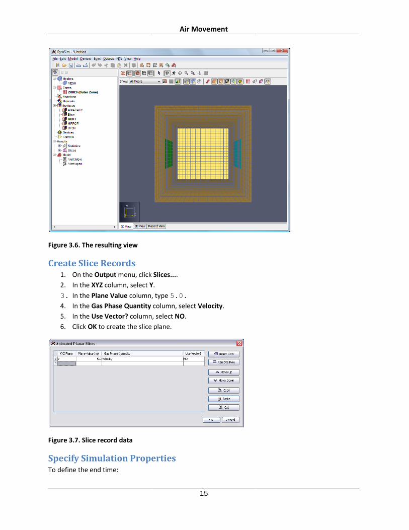
Create Slice Records 1. On the Output menu, click Slices....
2. In the XYZ column, select Y.
3. In the Plane Value column, type 5.0.
4. In the Gas Phase Quantity column, select Velocity.
5. In the Use Vector? column, select NO.
6. Click OK to create the slice plane.
Figure 3.7. Slice record data
Specify Simulation Properties To define the end time:
Air Movement
16
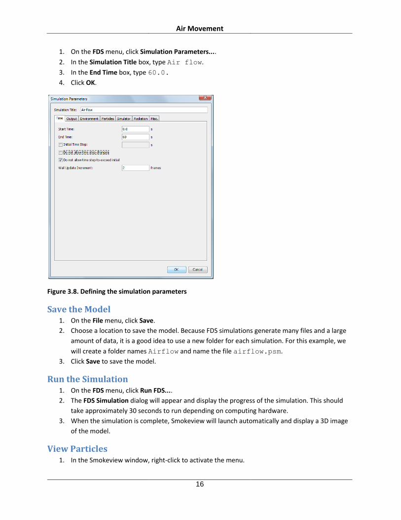
1. On the FDS menu, click Simulation Parameters....
2. In the Simulation Title box, type Air flow.
3. In the End Time box, type 60.0.
4. Click OK.
Figure 3.8. Defining the simulation parameters
Save the Model 1. On the File menu, click Save.
2. Choose a location to save the model. Because FDS simulations generate many files and a large
amount of data, it is a good idea to use a new folder for each simulation. For this example, we
will create a folder names Airflow and name the file airflow.psm.
3. Click Save to save the model.
Run the Simulation 1. On the FDS menu, click Run FDS....
2. The FDS Simulation dialog will appear and display the progress of the simulation. This should
take approximately 30 seconds to run depending on computing hardware.
3. When the simulation is complete, Smokeview will launch automatically and display a 3D image
of the model.
View Particles 1. In the Smokeview window, right-click to activate the menu.

Air Movement
17
2. In the menu, click Load/Unload > Particle File > particles to load the particle data.
View Slice Data 1. In the Smokeview window, right-click to activate the menu.
2. In the menu, click Load/Unload > Slice File > Velocity > Y=5.0.
Unload the particle data to view only the velocity contours.
Figure 3.9. View in Smokeview
Figure 3.10. View in Smokeview of velocity contours

Smoke Layer Height and Heat Flow Through a Door
18
Chapter 4. Smoke Layer Height and Heat Flow Through a
Door In this tutorial you will simulate an 800 kW fire in the corner of a 5m x 5m room. The room has a 1m
doorway. You will learn how to measure smoke layer height in the compartment and heat flow though
the doorway.
In this tutorial you will:
Create an 800 kW burner fire.
Create a doorway using a hole.
Add a flow measurement device.
Add a layer zoning device (to measure layer height).
View 3D results using Smokeview.
View 2D results using PyroSim.
Figure 4.1. Smoke in the model
Before you begin, ensure that you are using SI units (see Chapter 1).
Create the Burner Surface Surfaces are used to define the properties of objects in your FDS model. In this example, we define a
burner surface that releases heat at a rate of 800 kW/m2.
1. On the Model menu, click Edit Surfaces....
2. Click New....
3. In the Surface Name box, type burner, Figure 5.2.
4. In the Surface Type list, select Burner.
5. Click OK to create the new default burner surface.

Smoke Layer Height and Heat Flow Through a Door
19
Figure 4.2. Creating a new burner surface
1. In the Description box, type 800 kW/m2 burner, Figure 5.3
2. In the Heat Release Rate (HRR) box, type 800.
3. Click OK to save changes and close the Edit Surfaces dialog.
Figure 4.3. Defining parameters for the burner surface
Create the Burner Vent Vents have general usage in FDS to describe 2D planar objects. Taken literally, a vent can be used to
model components of the ventilation system in a building, like a diffuser or a return. In these cases, the
vent coordinates define a plane forming the boundary of the duct. No holes need to be created; air is
supplied or exhausted by the vent.
You can also use vents as a means of applying a particular boundary condition to a rectangular patch on
a surface. A fire, for example, can be created by specifying a vent on either a mesh boundary or solid
surface. The vent surface defines the desired characteristics of fire. This is the approach used in this
example.
Smoke Layer Height and Heat Flow Through a Door
20
1. On the Model menu, click New Vent....
2. In the Description box, type burner vent, Figure 5.4.
3. In the Surface list, select burner. This specifies that the previously created burner surface will
define the properties of the vent.
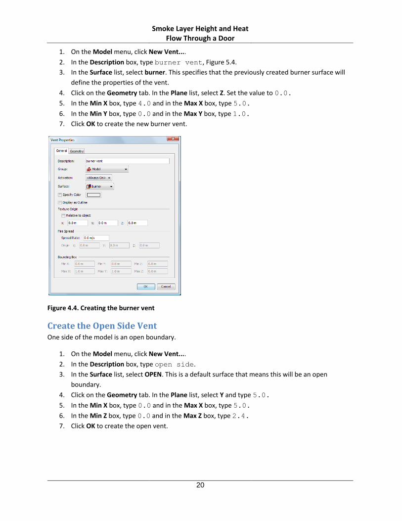
4. Click on the Geometry tab. In the Plane list, select Z. Set the value to 0.0.
5. In the Min X box, type 4.0 and in the Max X box, type 5.0.
6. In the Min Y box, type 0.0 and in the Max Y box, type 1.0.
7. Click OK to create the new burner vent.
Figure 4.4. Creating the burner vent
Create the Open Side Vent One side of the model is an open boundary.
1. On the Model menu, click New Vent....
2. In the Description box, type open side.
3. In the Surface list, select OPEN. This is a default surface that means this will be an open
boundary.
4. Click on the Geometry tab. In the Plane list, select Y and type 5.0.
5. In the Min X box, type 0.0 and in the Max X box, type 5.0.
6. In the Min Z box, type 0.0 and in the Max Z box, type 2.4.
7. Click OK to create the open vent.

Smoke Layer Height and Heat Flow Through a Door
21
Create the Mesh In this example we will use mesh cells that are 0.17 m across. This value is approximately 1/5 of the
characteristic diameter (D*) for a 800 kW fire. As a rule of thumb, this is as large as the mesh cells can be
while still maintaining a moderate level of accuracy in modeling the plume, (McGrattan, et al., 2007).
Using mesh cells that are smaller by a factor of 2 should decrease error by a factor of 4, but will increase
the simulation run time by a factor of 16.
1. On the Model menu, click Edit Meshes....
2. Click New
3. Click OK to create the new mesh. The boundary dimensions will automatically be set to the
correct size based on the two vents (Figure 5.5).
4. In the X Cells box, type 30.
5. In the Y Cells box, type 30.
6. In the Z Cells box, type 15.
7. Click OK to save changes and close the Edit Meshes dialog.
Figure 4.5. Creating the mesh
Add the Wall In FDS obstructions are used to define solid object in the model. In this example, we will use an
obstruction to define a wall.
1. On the Model menu, click New Obstruction....
2. In the Description box, type wall.
3. Click on the Geometry tab, Figure 5.6.

Smoke Layer Height and Heat Flow Through a Door
22
4. In the Min X box, type 0.0 and in the Max X box, type 5.0.
5. In the Min Y box, type 4.0 and in the Max Y box, type 4.2.
6. In the Min Z box, type 0.0 and in the Max Z box, type 2.4.
7. Click OK to create the wall obstruction.
Figure 4.6. Creating the wall
Add the Door 1. In FDS holes are used to define openings through solid objects. In this example, we will use a
hole to define a door.
2. On the Model menu, click New Hole....
3. In the Description box, type door.
4. Click on the Geometry tab. In the Min X box, type 2.0 and in the Max X box, type 3.0.
5. In the Min Y box, type 3.9 and in the Max Y box, type 4.3.
6. In the Min Z box, type 0.0 and in the Max Z box, type 2.0.
7. Click OK to create the doorway hole.
Orbit the Model for a Better View 1. To reset the zoom and properly center the model, press CTRL + R. PyroSim will now be looking
straight down at the model along the Z axis.

Smoke Layer Height and Heat Flow Through a Door
23
2. Press the left mouse button in the 3D View and drag to orbit the model. You can also unselect
the Show Holes button so that the hole object will not be displayed and you will just see the
opening through the wall.
Figure 4.7. The model after rotating. The burner is shown in red and the top vent in blue.
Add a Layer Zoning Device 1. On the Devices menu, click New Layer Zoning Device....
2. In the Device Name box, type layer zone 01.
3. For the End Point 1 coordinates, in the X box, type 2.5, in the Y box, type 2.5, and in the Z box,
type 0.0.
4. For the End Point 2 coordinates, in the X box, type 2.5, in the Y box, type 2.5, and in the Z box,
type 2.4.
5. Click OK to create the layer zoning device. It will be displayed as a line in the model.
Add a Flow Measuring Device 1. On the Devices menu, click New Flow Measuring Device....
2. In the Device Name box, type door flow.
3. In the Quantity options, select Heat Flow.
4. In the Plane list, select Y and type 4.0.
5. In the Min X box, type 2.0 and in the Max X box, type 3.0.
6. In the Min Z box, type 0.0 and in the Max Z box, type 2.0.
7. Click OK to create the flow measuring device. It will appear as a yellow plane in the model.

Smoke Layer Height and Heat Flow Through a Door
24
Set the Simulation Time 1. On the FDS menu, click Simulation Parameters....
2. On the Time panel, in the End Time box, type 45.0.
3. Click OK to save the simulation parameters.
Save the model 1. On the File menu, click Save.
2. Choose a location to save the model. Because FDS simulations generate many files and a large
amount of data, it is a good idea to use a new folder for each simulation. For this example, we
will create a Smoke folder and name the file smoke.psm.
3. Click OK to save the model.
Run the Simulation 1. On the FDS menu, click Run FDS....
2. The FDS Simulation dialog will appear and display the progress of the simulation. By default,
PyroSim specifies a 10 second simulation. This should take approximately 1 minute to run
depending on computing hardware, Figure 5.8.
3. When the simulation is complete, Smokeview should launch automatically and display a 3D still
image of the model, Figure 5.9.
Figure 4.8. The simulation dialog during the analysis.

Smoke Layer Height and Heat Flow Through a Door
25
Figure 4.9. The initial Smokeview display.
View Smoke in 3D 1. In the Smokeview window, right-click to activate the menu.
2. In the menu, click Load/Unload > 3D Smoke > soot mass fraction (RLE). This will start an
animation of the smoke in this model.
3. In the menu, click Load/Unload > 3D Smoke > HRRPUV (RLE). This will start add an animation of
fire to the model in addition to the smoke.
4. To view a specific time in the animation, click the timeline bar in the bottom of the Smokeview
window. To return to animation mode, press t.
5. To reset Smokeview, right-click to activate the menu, then click Load/Unload > Unload All.
Figure 4.10. 3D smoke in the model.
Smoke Layer Height and Heat Flow Through a Door
26
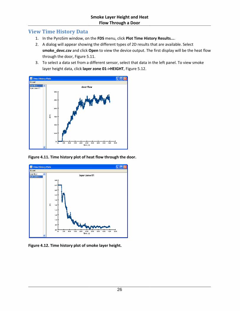
View Time History Data 1. In the PyroSim window, on the FDS menu, click Plot Time History Results....
2. A dialog will appear showing the different types of 2D results that are available. Select
smoke_devc.csv and click Open to view the device output. The first display will be the heat flow
through the door, Figure 5.11.
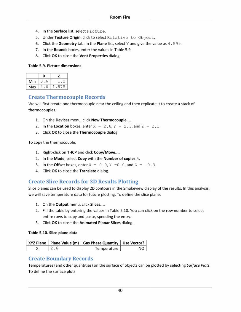
3. To select a data set from a different sensor, select that data in the left panel. To view smoke
layer height data, click layer zone 01->HEIGHT, Figure 5.12.
Figure 4.11. Time history plot of heat flow through the door.
Figure 4.12. Time history plot of smoke layer height.

Room Fire
27
Chapter 5. Room Fire This tutorial demonstrates how to:
Import properties from a database.
Define a combustion reaction.
Replicate and rotate obstructions (furniture).
Use a hole to represent an open door.
Define an open surface on the exterior of the model.
View 3D results using Smokeview.
View 2D results using PyroSim.
Figure 5.1. Room fire in this example
This example is a simplification of the Roomfire problem provided as an FDS verification problem. You
can download the complete FDS verification file at: http://fds-
smv.googlecode.com/svn/trunk/FDS/trunk/Verification/Fires/room_fire.fds, then import this file into
PyroSim.
Import Reaction and Material Data PyroSim includes a database file that includes references for the source of the data. We will import
selected properties from this file.
1. On the Model menu, click Edit Libraries....
2. In the Category box, select Gas-phase Reactions.
3. Copy the POLYURETHANE reaction from the library into the Current Model.
4. In the Category box, select Materials.

Room Fire
28
5. Copy the FOAM, GYPSUM, and YELLOW PINE materials from the library into the Current Model.
6. Close the PyroSim Libraries dialog.
Figure 5.2. Copy the reaction from the library
Save the Model This is a good time to save the model.
1. On the File menu, click Save.
2. Choose a location to save the model. Because FDS simulations generate many files and a large
amount of data, it is a good idea to use a new folder for each simulation. Name the file
roomfire.psm.
3. Click OK to save the model.
Create the Mesh In this example we will use mesh cells with a size of 0.10 m. This is geometrically convenient and is fine
enough relative to the burner HRR to give moderate numerical accuracy.
1. On the Model menu, click Edit Meshes....
2. Click New and then OK to create a new mesh, see Figure 5.3
3. In the Min X box, type 0.0 and in the Max X box, type 5.2.
4. In the Min Y box, type -0.8 and in the Max Y box, type 4.6.
5. In the Min Z box, type 0.0 and in the Max Z box, type 2.4.
6. In the X Cells box, type 52.
7. In the Y Cells box, type 54.

Room Fire
29
8. In the Z Cells box, type 24.
9. Click OK to save changes and close the Edit Meshes dialog.
Figure 5.3. Creating the mesh
Specify Combustion Parameters Since there is only one reaction in the model, by default that will be the reaction used for the analysis.
No other action is necessary.
You can double-click on POLYURETHANE to display the properties, Figure 5.4.

Room Fire
30
Figure 5.4. The POLYURETHANE reaction parameters.
Click the Cancel button to close the Edit Reactions dialog.
Create Surfaces Materials, which we have already imported, define physical properties. Surfaces that represent solid
objects in the model use the material properties. Vent and burner surfaces are defined directly, without
reference to materials.
The floor will be made of yellow pine. To create the surface:
1. On the Model menu, click Edit Surfaces....
2. Click New, give the Surface Name as Pine, select the Surface Type as Layered, and click OK.
3. Click on the Texture box and select psm_spruce.jpg. Click OK to close the Texture dialog.
4. In the Material Layers panel, in the Thickness column, type 0.01.
5. The material composition can be defined as a mixture. Click the Edit button. In the Mass
Fraction column, type 1.0. In the Material column, select YELLOW PINE. Click OK to close
the Composition dialog.
6. In the Edit Surfaces dialog, click Apply to save the changes.

Room Fire
31
Figure 5.5. Creating the floor surface.
We will use gypsum for the walls:
1. In the Edit Surfaces dialog, click New... Give the Surface Name as Gypsum, select the Surface
Type as Layered, and click OK.
2. Click on the Color box and select a gray color (e.g. RGB of 0.7, 0.7, 0.7). Click OK to close the
Surface Color dialog.
3. In the Material Layers panel, in the Thickness column, type 0.013.
4. Click the Edit button. In the Mass Fraction column, type 1.0. In the Material column, select
GYPSUM. Click OK to close the Composition dialog.
5. In the Edit Surfaces dialog, click Apply to save the changes.
For the upholstery:
1. In the Edit Surfaces dialog, click New. Give the Surface Name as Upholstery, select the
Surface Type as Layered, and click OK.
2. Click on the Color box and select a color (e.g. RGB of 0.4, 0.2, 0.0). Click OK to close the Surface
Color dialog.
3. In the Material Layers panel, in the Thickness column, type 0.1.
4. Click the Edit button. In the Mass Fraction column, type 1.0. In the Material column, select
FOAM. Click OK to close the Composition dialog.
5. Click on the Surface Props tab. In the Backing box, select Insulated.
6. Click on the Reaction tab. Select Allow the Obstruction to Burn Away. When this option is
selected, the solid object disappears from the calculation cell by cell, as the mass contained by
each mesh cells is consumed either by the pyrolysis reactions or by the prescribed HRR.

Room Fire
32
7. In the Edit Surfaces dialog, click Apply to save the changes.
We will place an initial burner surface on the sofa. The burner will release heat at a constant rate that
will ignite the upholstery. To create this burner surface:
1. In the Edit Surfaces dialog, click New. Give the Surface Name as Burner, select the Surface
Type as Burner, and click OK.
2. In the Heat Release panel, in the Heat Release Rate (HRR) box, type 1000.
3. In the Edit Surfaces dialog, click OK to save the changes and close the dialog.
Create Furniture (Obstructions) We will now create some furniture to place in the model.
Couch
The first will be a couch. Create a Couch group that will help us organize the input.
1. On the Model menu, click New Group....
2. In the Parent Group list, select Model.
3. In the Group Name box, type Couch.
4. Click OK to close the Create Group dialog.
To create the couch base:
1. On the Model menu, click New Obstruction....
2. In the Description box, type Base.
3. In the Group list, select Couch.
4. Click on the Geometry tab. In the Box Properties boxes, enter the values in Table 5.1, see Figure
5.6.
5. Click on the Surfaces tab. Select Single and select Gypsum from the list.
6. Click OK to close the Obstruction Properties dialog.
Table 5.1. Couch base dimensions
X Y Z
Min 1.5 3.8 0.0
Max 3.1 4.6 0.4

Room Fire
33
Figure 5.6. Input for the couch base
To create the seat:
1. On the Model menu, click New Obstruction....
2. In the Description box, type Seat cushion.
3. In the Group list, select Couch.
4. On the Geometry tab, enter the values in Table 5.2.
5. On the Surfaces tab, select Single and select Upholstery from the list.
6. Click OK to close the Obstruction Properties dialog.
Table 5.2. Couch seat dimensions
X Y Z
Min 1.5 3.8 0.4
Max 3.1 4.6 0.6
To create an armrest:
1. On the Model menu, click New Obstruction....
2. In the Description box, type Right armrest.
3. In the Group list, select Couch.
4. On the Geometry tab, enter the values in Table 5.3.
5. On the Surfaces tab, select Single and select Upholstery from the list.
6. Click OK to close the Obstruction Properties dialog.

Room Fire
34
Table 5.3. Right armrest dimensions
X Y Z
Min 1.3 3.8 0.0
Max 1.5 4.6 0.9
We will use the copy function to create the other armrest.
1. Right-click the Right armrest either in the Tree View or the 3D view.
2. Click Copy/Move.
3. In the Mode options, select Copy with 1 copy.
4. In the Offset boxes, enter X = 1.8, Y = 0.0, and Z = 0.0.
5. Click OK to close the Translate dialog.
By default, the name given to the armrest copy will be Right armrest[1], where the [1] indicates
the first copy. To rename, double-click on the Right armrest[1] in the Tree view and change the
Description to Left armrest. Click OK.
To create the back:
1. On the Model menu, click New Obstruction....
2. In the Description box, type Back cushion.
3. In the Group list, select Couch.
4. On the Geometry tab, enter the values in Table 5.4.
5. On the Surfaces tab, select Single and select Upholstery from the list.
6. Click OK to close the Obstruction Properties dialog.
Table 5.4. Couch back dimensions
X Y Z
Min 1.5 4.4 0.6
Max 3.1 4.6 1.2
The display will appear as shown in

Room Fire
35
Figure 5.7. The room after the couch is added
Second Couch
We will now create a second couch using the copy function.
1. In the Tree View, right-click the Couch group.
2. Click Copy/Move.
3. In the Mode options, select Copy with 1 copy.
4. In the Offset boxes, enter X = -1.3, Y = -3.6, and Z = 0.0.
5. Click OK to close the Translate dialog.
Rename Couch[1] to Couch 2.
Rotate the second couch to lie against the well.
1. In the Tree View, right-click Couch 2 group.
2. Click Rotate....
3. In the Mode options, select Move.
4. In the Angle box, type 90.
5. In the Base Point boxes, enter X = 0.0 and Y = 1.0.
6. Click OK to close the Rotate Objects dialog.
Additional Furniture
Add a pad:
1. On the Model menu, click New Obstruction....
2. In the Description box, type Pad.
3. In the Group list, select Model.
4. On the Geometry tab, enter the values in Table 5.5.

Room Fire
36
5. On the Surfaces tab, select Single and select Upholstery from the list.
6. Click OK to close the Obstruction Properties dialog.
Table 5.5. Table Dimensions
X Y Z
Min 1.6 2.4 0.0
Max 3.0 3.2 0.2
The resulting room display is shown in Figure 5.8.
Figure 5.8. The resulting room display
Constucting complex objects can be time consuming. If your geometry is available in DXF format,
PyroSim supports import. For walls, PyroSim provides sketching on a background image. Alternately, if
you use the same geometry in many models, you can create the geometry and save it. You can then
copy any object from one model to another. You can even copy just the text from an FDS input file and
paste it into a PyroSim model.
Walls We will add a wall using the 2D View. Since we will be adding only one wall, this wall could also be
added quickly as a single obstruction. However, we will use the 2D view in order to demonstrate its use.
1. Select the 2D View.
2. Select the Wall ( ) Tool.
3. Select the Tool Properties ( ) icon. Set the Z Location to 0.0, the Thickness to 0.24, the
Height to 2.4, and change the Surface Prop to Gypsum. Click OK.

Room Fire
37
4. With the wall tool draw the wall from left to right along the Y=0 line. Right click and select Finish
to exit the drawing tool. Hold down the Shift key to position the wall in the lower part of the
model, Error! Reference source not found..
Figure 5.9. Drawing the wall
Create Door (Hole in Wall) To add a door by creating a hole in the wall:
1. On the Model menu, click New Hole....
2. In the Description box, type Door.
3. In the Group list, select Model.
4. On the Geometry tab, enter the values in Table 5.6. Note that we extend the hole beyond the
bounds of the wall it intersects. This ensures the hole will take priority over the wall.
5. Click OK to close the Obstruction Properties dialog.
Table 5.6. Door Dimensions
X Y Z
Min 4.0 -0.3 0.0
Max 4.9 0.1 2.0
The model now looks like:

Room Fire
38
Figure 5.10. The model after adding the door
Use Vents to Define the Burner Fire and Floor In FDS, Vents are used to describe 2D planar objects. In this example, we use vents to define the burner
fire and the carpet on the floor.
Create the Fire
The fire is ignited by a burner that releases heat at a fixed rate. The adjacent material eventually reaches
ignition temperature and begins to burn. Here, we use a vent for the burner fire on the couch.
1. On the Model menu, click New Vent....
2. In the Description box, type Burner.
3. In the Group list, select Model.
4. In the Surface list, select Burner.
5. Click the Geometry tab. In the Plane list, select Z and give the value as 0.601 (The small value
greater than 0.6 ensures the vent is displayed above the couch.).
6. In the Bounds boxes, enter the values in Table 5.7.
7. Click OK to close the Vent Properties dialog.
Table 5.7. Burner fire dimensions
X Y
Min 2.5 4.1
Max 2.7 4.4
Floor
The floor is also represented as a vent.
1. On the Model menu, click New Vent....

Room Fire
39
2. In the Description box, type Floor.
3. In the Group list, select Model.
4. In the Surface list, select Pine.
5. Click on the Geometry tab. In the Plane list, select Z and give the value as 0.001.
6. In the Bounds boxes, enter the values in Table 5.8.
7. Click OK to close the Vent Properties dialog.
Table 5.8. Open boundary dimensions
X Y
Min 0.0 0.0
Max 5.2 4.6
Add an Open Boundary We will add an open boundary on the model outside the door. PyroSim provides a shortcut that can
create open vents on mesh boundaries.
1. In the navigation view, right-click on the MESH and click Open Mesh Boundaries. This will add a
group named Vents for MESH that includes vents on each grid boundary.
2. Holding the CNTRL key, click on all Grid Boundary Vents except the Vent Min Y for MESH.
3. Right-click and delete the selected vents.
4. Right-click on the Model and select Show All Objects.
Hang a Picture to the Wall Let us hang a picture on the wall. First decide what picture you want to hang.
1. On the Model menu, click Edit Surfaces....
2. In the Edit Surfaces dialog, click New. Give the Surface Name as Picture, select the Surface
Type as Adiabatic, and click OK.
3. Click on the Texture box.
4. Click the Import... button and select the image you want as a picture. I used the image call
motorcycle.jpg that is included in the PyroSim installation in the samples folder (C:\ Program
Files\ PyroSim 2012\ samples).
5. The image you selected will be displayed. Under the image, click the Details tab. Deselect the
Lock aspect ratio checkbox, then set the Width to 1.0 and the Height to 0.675 (or whatever
values are appropriate for your image.)
6. Click OK to close the Textures dialog.
7. Click OK to close the Edit Surfaces dialog.
We now create a vent that uses the texture.
1. On the Model menu, click New Vent....
2. In the Description box, type Picture.
3. In the Group list, select Model.
Room Fire
40
4. In the Surface list, select Picture.
5. Under Texture Origin, click to select Relative to Object.
6. Click the Geometry tab. In the Plane list, select Y and give the value as 4.599.
7. In the Bounds boxes, enter the values in Table 5.9.
8. Click OK to close the Vent Properties dialog.
Table 5.9. Picture dimensions
X Z
Min 3.6 1.2
Max 4.6 1.875
Create Thermocouple Records We will first create one thermocouple near the ceiling and then replicate it to create a stack of
thermocouples.
1. On the Devices menu, click New Thermocouple....
2. In the Location boxes, enter X = 2.6, Y = 2.3, and Z = 2.1.
3. Click OK to close the Thermocouple dialog.
To copy the thermocouple:
1. Right-click on THCP and click Copy/Move....
2. In the Mode, select Copy with the Number of copies 5.
3. In the Offset boxes, enter X = 0.0, Y =0.0, and Z = -0.3.
4. Click OK to close the Translate dialog.
Create Slice Records for 3D Results Plotting Slice planes can be used to display 2D contours in the Smokeview display of the results. In this analysis,
we will save temperature data for future plotting. To define the slice plane:
1. On the Output menu, click Slices....
2. Fill the table by entering the values in Table 5.10. You can click on the row number to select
entire rows to copy and paste, speeding the entry.
3. Click OK to close the Animated Planar Slices dialog.
Table 5.10. Slice plane data
XYZ Plane Plane Value (m) Gas Phase Quantity Use Vector?
X 2.6 Temperature NO
Create Boundary Records Temperatures (and other quantities) on the surface of objects can be plotted by selecting Surface Plots.
To define the surface plots

Room Fire
41
1. On the Output menu, click Boundary Quantities....
2. Click the Wall Temperature checkbox.
3. Click OK to close the Animated Boundary Quantities dialog.
Specify Simulation Properties To define the end time:
1. On the FDS menu, click Simulation Parameters....
2. In the Simulation Title box, type Room fire.
3. In the End Time box, type 600 s.
4. Click OK.
The Model is Completed Your model should now look like Figure 5.11. Save it.
Figure 5.11. Completed model
Run the Analysis To run the analysis:
1. On the FDS menu, click Run FDS.... The analysis will take about four hours to run on a 2.0 GHz
computer.

Room Fire
42
View the Results You can use the Smokeview software to make plots of the results. In Smokeview, on the Show/Hide
menu click Textures and then select Show All to display all the textures, An image showing the heat
release rate isosurface and temperature contours on the slice plane is shown in Figure 5.12. Notice that
the couch is burning away.
Figure 5.12. Heat release rate isosurface and temperature contours
To view time history results
1. In the PyroSim window, on the FDS menu, click Plot Time History Results....
2. A dialog will appear showing a list of 2D result files. Select roomfire_hrr.csv and click Open to
view the heat release rate as a function of time, Figure 5.13.

Room Fire
43
Figure 5.13. Heat release rate

Switchgear Fire Example
44
Chapter 6. Switchgear Fire Example This example evaluates fire conditions in two adjacent switchgear rooms connected by a double fire
door, Figure 6.1 The figure shows switchgear cabinets, cable trays, supply ducts and vents, and smoke
detectors. The drawing is not to scale. In the fire scenario, a fire starts in a switchgear cabinet in room
3A. The fire modeling results will used to estimate the time available for operators to conduct manual
actions in one of the switchgear rooms. This example was provided by Bryan Klein (Klein, 2007).
Figure 6.1. Pictorial representation of the switchgear room complex
This tutorial demonstrates how to:
Define materials.
Create and replicate geometry.
Open doors after a specified time.
Create a burner fire.
Add a smoke layer device.
Add a slice plane for temperature visualization.
View 3D results using Smokeview.
View 2D results using PyroSim.

Switchgear Fire Example
45
Figure 6.2. Completed model
Model parameters are given below.
Table 6.1. Room size (interior dimensions)
Dimension English Metric
Length 28’-6” 8.6 m
Width 28”-6” 8.6 m
Height 20’ 6.0 m
Wall Thickness 2’ 0.6096 m
Table 6.2. Door size
Dimension English Metric
Width 3’ 0.9 m
Height 8’ 2.4 m
Table 6.3. Concrete properties (NBSIR 88-3752)
Property Value
Density 2280
kg/m^3
Specific Heat 1.04
kJ/kg-K
Conductivity 1.8 W/m-K
Table 6.4. Sheet metal properties (Drysdale, Intro to Fire Dynamics)
Property Value
Switchgear Fire Example
46
Density 7850 kg/m^3
Specific Heat 0.46 kJ/kg-K
Conductivity 45.8 W/m-k
Table 6.5. Cable properties (NUREG/CR-6850)
Property Value
Density 1380 kg/m^3
Specific Heat 1.289 kJ/kg-K
Conductivity 0.192 W/m-k
Computational Mesh In this example, we will use two meshes. We will use relatively coarse meshes that should be refined for
a final analysis. In Room 3A (the room on the right) the cell size will be approximately 0.5 ft (0.1524 m)
and in Room 3B, approximately 1.0 ft (0.3048 m). We have selected a finer resolution in Room 3A to
more accurately represent the geometry of the cable trays and to provide a finer resolution for the flow
solution near the fire. The two meshes much touch in order to transfer information between them. We
will position the common plane inside Room 3B, so that the finer mesh includes all of Room 3A and the
door between the rooms.
There is always a compromise between number of cells and acceptable solution time. As described, this
model will have 162 000 cells and run in approximately 8 hours on a single CPU computer.
This problem uses English units as the primary values for the geometry. Switch to English units:
1. On the View menu, click Units.
2. Select English.
To create the first solution mesh for Room 3A:
1. On the Model menu, click Edit Meshes....
2. Click New to create a mesh.
3. In the Name box, type Room 3A. Click OK to close the New mesh dialog.
4. In the Order/Priority list, select 1. This ensures that the finer mesh is the primary mesh for the
solution.
5. In the Mesh Boundary boxes, enter the values in Table 6.6.
6. In the X, Y, and Z cell boxes, enter 60, enter 60, and enter 40 respectively, as shown in Figure
6.3. The FDS solution is optimized when the mesh cell division is defined by a number that can
be formed using multiples of powers of 2, 3 and 5. These divisions give a cell size of
approximately 0.5 ft (0.1524 m).
7. Click Apply to create the mesh.
Table 6.6. Dimensions for the mesh in Room 3A (including 2' thick walls)
X (ft) Y (ft) Z (ft)

Switchgear Fire Example
47
Min 27.5 0.0 0.0
Max 59.0 28.5 20.0
Figure 6.3. Input to create the mesh
To create the second solution mesh for Room 3B:
1. Click New to create a mesh.
2. In the Name box, type Room 3B. Click OK to close the New mesh dialog.
3. In the Order/Priority list, select 2.
4. In the Mesh Boundary boxes, enter the values in Table 6.7.
5. In the X, Y, and Z cell boxes, enter 30, enter 30, and enter 20 respectively. These divisions give
a cell size of approximately 1.0 ft (0.3048 m).
6. Click OK to save the data close the Edit Meshes dialog.
Table 6.7. Dimensions for the mesh in Room 3B (including 2' thick walls)
X (ft) Y (ft) Z (ft)
Min 0.0 0.0 0.0
Max 27.5 28.5 20.0
The meshes are shown in Figure 6.4. On the toolbar, click to reset the image. Click . You can orbit,
pan, and zoom the model using the mouse and the Shift and Alt keys.

Switchgear Fire Example
48
Figure 6.4. Display of the meshes
Material Properties FDS uses materials to define physical properties. In this model, we will include the following material
types: concrete, steel, and thermo-plastic cable. PyroSim includes a database file with material data and
the references from which that data was obtained. We will import the concrete and steel material
properties from this file.
1. On the Model menu, click Edit Libraries....
2. In the Category box, select Materials.
3. Use the arrow to copy the CONCRETE and STEEL materials from the library into the Current
Model, Figure 6.5.
4. Close the PyroSim Libraries dialog.

Switchgear Fire Example
49
Figure 6.5. Copy the material data from the library to the model
We will enter the material properties for the cable manually. We note that the material properties in the
problem description have been provided in metric units, so we will temporarily switch to metric units:
1. On the View menu, click Units.
2. Select SI.
The cables will be represented as a thermo-plastic material:
1. On the Model menu, click Edit Materials....
2. In the Edit Materials...dialog, click New....
3. In the Material Name box, type Cable, in the Material Type list, select Solid. Click OK to
close the New Material dialog.
4. In the Density box, type 1380 kg/m^3, Figure 6.6.
5. In the Specific Heat box, type 1.289 kJ/kg-K,
6. In the Conductivity box, type 0.192 W/m-K,
7. Click OK to save the changes and close the Edit Materials dialog.

Switchgear Fire Example
50
Figure 6.6. Thermo-plastic properties
Save the Model This is a good time to save the model.
1. On the File menu, click Save.
2. Choose a location to save the model. Because FDS simulations generate many files and a large
amount of data, it is a good idea to use a new folder for each simulation. For this example, we
will name the file C:\ Switchgear\ switchgear.psm.
3. Click OK to save the model.
Surface Properties Surfaces are used to define the properties of objects in your model. Solid surfaces will use the material
properties previously defined.
This problem uses English units as the primary values for the geometry. Switch to English units.
1. On the View menu, click Units.
2. Select English.
The concrete wall is 2 ft (0.6096 m) thick. This will be a Layered surface, although we will define only
one layer. To create this surface
1. On the Model menu, click Edit Surfaces....
2. Click New....
3. In the Surface Name box, type Concrete Wall, in the Surface Type list, select Layered.
Click OK to create the surface and close the New Surface dialog.
4. Click the Color button to open the Surface Color dialog, then select a dark gray and click OK.
5. In the Material Layers panel, in the Thickness column, type 2.0 ft.
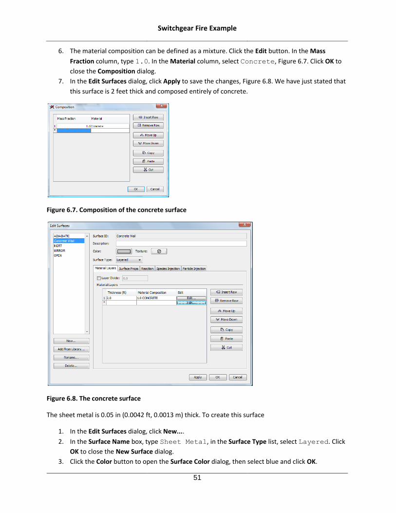
Switchgear Fire Example
51
6. The material composition can be defined as a mixture. Click the Edit button. In the Mass
Fraction column, type 1.0. In the Material column, select Concrete, Figure 6.7. Click OK to
close the Composition dialog.
7. In the Edit Surfaces dialog, click Apply to save the changes, Figure 6.8. We have just stated that
this surface is 2 feet thick and composed entirely of concrete.
Figure 6.7. Composition of the concrete surface
Figure 6.8. The concrete surface
The sheet metal is 0.05 in (0.0042 ft, 0.0013 m) thick. To create this surface
1. In the Edit Surfaces dialog, click New....
2. In the Surface Name box, type Sheet Metal, in the Surface Type list, select Layered. Click
OK to close the New Surface dialog.
3. Click the Color button to open the Surface Color dialog, then select blue and click OK.

Switchgear Fire Example
52
4. In the Material Layers panel, in the Thickness column, type 0.0042 ft.
5. The material composition can be defined as a mixture. Click the Edit button. In the Mass
Fraction column, type 1.0. In the Material column, select Steel. Click OK to close the
Composition dialog.
6. In the Edit Surfaces dialog, click Apply to save the changes.
The cable is 1.5 in (0.125 ft, 0.0381 m) thick. To create this surface
1. In the Edit Surfaces dialog, click New....
2. In the Surface Name box, type Cable, in the Surface Type list, select Layered. Click OK to
close the New Surface dialog.
3. Click the Color button to open the Surface Color dialog, then select a black and click OK.
4. In the Material Layers panel, in the Thickness column, type 0.125 ft.
5. The material composition can be defined as a mixture. Click the Edit button. In the Mass
Fraction column, type 1.0. In the Material column, select Cable. Click OK to close the
Composition dialog.
6. Click on the Surface Props tab. In the Backing list, select Insulated. This will approximate a
solid being heated from all sides.
7. Click OK to close the Edit Surfaces dialog.
Switch to SI units to input additional properties given in SI units.
1. On the View menu, click Units.
2. Select SI.
Edit the heat release rate and ignition temperature for the Cable surface. These values should only be
considered as examples.
1. Right-click on Cable in the Surfaces list. Click Properties.
2. Click the Reaction tab.
3. Click to select Governed Manually.
4. In the Heat Release Rate box, type 265 kW/m^2. In the Ignition panel select Ignite at and type
250 C.
5. Click OK to save the changes and close the Edit Surfaces dialog.
Model Geometry We will now create the geometry using a few dialogs and by drawing a few walls. If you were working on
a more complex building, you could display the floor plan in the 2D View and then sketch walls directly
on the background image or import the data from a DXF file.
The model will only include the separating wall between the two rooms. There is no need to define the
perimeter walls, since the perimeter will be assigned the surface properties of the concrete wall.

Switchgear Fire Example
53
During the creation of a PyroSim model, it is recommended that you group the various parts of the
model for purposes of editing and later viewing. For example, all walls will be placed in a sub-group
called Walls. This allows us to quickly select this group to modify it or to hide it for viewing of other
interior details.
The problem dimensions use English units as the primary values. To switch to English units
1. On the View menu, click Units.
2. Select English.
Walls and Doors
To make a new group:
1. On the Model menu, click New Group....
2. In the Parent Group list, select Model.
3. In the Group Name box, type Walls.
4. Click OK to close the Create Group dialog.
To define the dividing wall
1. On the Model menu, click New Obstruction....
2. In the Description box, type Dividing Wall.
3. In the Group list, select Walls.
4. Click on the Geometry tab. In the Bounding Box boxes, enter the values listed in Table 6.8 and
shown in Figure 6.9.
5. Click on the Surfaces tab, select Single and select Concrete Wall from the list.
6. Click OK to close the Obstruction Properties dialog.
7. In the toolbar, click to turn off the Show Mesh Divisions option. The display should now look
like Figure 6.10.
Table 6.8. Dividing wall dimensions
X (ft) Y (ft) Z (ft)
Min 28.5 0.0 0.0
Max 30.5 28.5 20.0

Switchgear Fire Example
54
Figure 6.9. Input for the wall dividing the two rooms
Figure 6.10. Display of the dividing wall
We will use a Hole obstruction to represent the door between the rooms. A hole can defined in the
model, but not activate until a specified time or event. In this case, we will define a hole (door) between

Switchgear Fire Example
55
the rooms that will open 5 minutes (300 seconds) after the start of the fire. To add the dividing door to
the model:
1. On the Model menu, click New Hole....
2. In the Description box, type Dividing Door.
3. In the Group list, select Walls.
4. Click on the Geometry tab. In the Bounding Box boxes, enter the values in Table 7.9. The values
are chosen thicker than the wall to ensure that the door takes precedence. In the toolbar, click
to turn off the Show Holes option. Now we just see the door through the wall.
5. Return to the General tab. Devices are used to link a response (i.e. open a door) to an event in
the model (i.e. a temperature measurement reaching a set value). In this model, we will open
the door after 300 seconds.
6. Click the Activation button. In the list, select New... to create a new device. For the Name type
Open Door. Click OK.
7. For the Input Type, select Time. For the Action to Perform, select Create/Activate. In the text
window, click on TBEGIN to change the time. In the pop-up box, type 300.0 s and press
ENTER on your keyboard. The control logic will now be displayed, Figure 6.11. Click OK to create
the control.
8. Click OK to close the Vent Properties dialog. You will notice that an Open Door control has been
added to Controls in the Navigation View.
Table 6.9. Dividing door dimensions
X (ft) Y (ft) Z (ft)
Min 28.5 11.25 0.0
Max 30.75 17.25 8.0

Switchgear Fire Example
56
Figure 6.11. The contol logic that opens the dividing door
We also will add the Room 3B entrance door. We want this door to stay closed for 300 sec. By default,
FDS assumes the boundary of a mesh is closed. To define a door on the boundary, we will first create an
open vent on the mesh boundary, then plug it with an obstruction that will be removed at 300 sec. To
add the entrance door to the model:
1. On the Model menu, click New Vent....
2. In the Description box, type Entrance Door.
3. In the Group list, select Walls.
4. In the Surface list, select OPEN.
5. Click on the Geometry tab. In the Lies in the Plane list, select Y and type 28.5.
6. In the Min X box, type 20.0 and in the Max X box, type 26.0.
7. In the Min Z box, type 0.0 and in the Max Z box, type 8.0.
8. Click OK to save the changes and close the Vent Properties dialog.
To define the blockage in the entrance door:
1. On the Model menu, click New Obstruction....
2. In the Description box, type Entrance Door Blockage.
3. In the Group list, select Walls.
4. Click on the Geometry tab. In the Bounding Box boxes, enter the values in Table 6.10. The
values are chosen thicker than the wall to ensure that the door takes precedence.
5. Click on Surfaces tab. Select Single and select Concrete Wall from the list.
6. Click the Activation button. In the list, select New... to create a new device. For the Name type
Entrance Blockage. Click OK.

Switchgear Fire Example
57
7. For the Input Type, select Time. For the Action to Perform, select Remove/Deactivate. In the
text window, click on TBEGIN to change the time. In the pop-up box, type 300.0 s and press
ENTER on your keyboard. Click OK to create the control.
8. Click OK to close the Obstruction Properties dialog. You will notice that an Entrance Blockage
control has been added to Controls in the Navigation View. This control will remove the
obstruction (open the door) at 300.0 seconds.
Table 6.10. Entrance door blockage dimensions
X (ft) Y (ft) Z (ft)
Min 19.5 28.0 0.0
Max 26.5 29.0 8.0
Switchgear Cabinets
First, make a switchgear group:
1. On the Model menu, click New Group....
2. In the Parent Group list, select Model.
3. In the Group Name box, type Switchgear.
4. Click OK to close the Create Group dialog.
We could define the cabinets using the New Obstruction... menu and dialog as described above. Instead
we will sketch the cabinets. To prepare to draw the switchgear cabinets:
1. Click 2D View.
2. On the View menu, click Snap to Sketch Grid. The Sketch Grid allows you to specify a
grid spacing that is useful for creating geometry independent of the solution meshes.
3. On the View menu, click Set Sketch Grid Spacing.... In the Snap Spacing box, type 0.5. Click OK
to close the Snap-to Grid dialog.
4. Use the Pan View tool to drag the model so that the dividing wall is to the right of the window.
To draw the cabinet:
1. In the 2D View drawing tools toolbar (left of window), click the Draw an Obstruction tool ( ).
2. To set the tool properties, click Tool Properties ( ).
3. In the Z Location box, type 0.0 and in the Thickness box, type 8.0. In the Surface Prop list,
select Sheet Metal. Click OK to close the New Obstruction Properties dialog.
4. In the 2D View action toolbar (top of window), select Switchgear in the Group list.
5. Press and drag the mouse, approximating the dimensions of the lower left cabinet shown in
Figure 6.1.
6. Your sketch will approximate that shown in Figure 6.12.

Switchgear Fire Example
58
Figure 6.12. Sketch of the lower left cabinet
By default, the cabinet sketch snapped to the sketch grid points. To precisely define the dimensions of
the cabinet
1. In the 2D View action toolbar (top of window), click the Select and Manipulate Objects tool
( ).
2. Double-click on the cabinet to edit its properties.
3. In the Description box, type Cabinet 1.
4. Click the Geometry tab. In the Bounding Box boxes, enter the values in Table 6.11.
5. Click OK to close the Obstruction Properties dialog.
Table 6.11. Cabinet Dimensions
X (ft) Y (ft) Z (ft)
Min 4.0 4.0 0.0
Max 20.0 10.0 8.0
We will now copy the first cabinet using the Translate Objects tool in the 2D View.
1. Using the Select and Manipulate Objects tool ( ), click on Cabinet 1.
2. Click the Translate Objects tool ( ).
3. Press the CTRL key (to create a copy) and drag upward to create a second cabinet, Figure 6.13.
4. Click the Select and Manipulate Objects tool ( ).

Switchgear Fire Example
59
5. Double click on the new cabinet and change the name to Cabinet 2. On the Geometry tab, set
the dimensions for Cabinet 2 given in Table 6.12.
Figure 6.13. Making a copy of Cabinet 1 by dragging. The final position will be 4 feet from the left and
top boundaries.
Table 6.12. Dimensions for Cabinet 2
X (ft) Y (ft) Z (ft)
Min 4.0 18.5 0.0
Max 20.0 24.5 8.0
We now copy both cabinets using the Copy/Move... menu. You could alternately use the Translate
Objects tool as before.
1. Using the Select and Manipulate Objects tool ( ), press CTRL and click on both Cabinet 1 and
Cabinet 2.
2. Right-click on either cabinet and click Copy/Move....
3. Click Copy and type 1 in the Number of Copies box.
4. In the Offset box for X, type 30.5 .
5. Click OK.
6. Change the cabinet names to Cabinet 3 and Cabinet 4.
The cabinets are shown in Figure 6.14.

Switchgear Fire Example
60
Figure 6.14. The rooms showing the switchgear cabinets
Cable Trays
The cables are supported by ladder trays. These trays are relatively open to air flow and have relatively
little thermal mass compared to the cables. Therefore, we will not model the details of the trays, but will
just model the cables. First, make a cables group:
1. On the Model menu, click New Group....
2. In the Parent Group list, select Model.
3. In the Group Name box, type Cables.
4. Click OK to close the Create Group dialog.
To prepare to draw the cables:
1. Click 2D View. This will display the sketch grid.
2. In the 2D View drawing tools toolbar (left of window), click the Draw an Obstruction tool ( ).
3. To set the tool properties, click Tool Properties ( ). In the Z Location box, type 8.5. In the
Thickness box, type 0.5. In the Surface Prop list, select Cable. Click OK to close the New
Obstruction Properties dialog.
4. In the 2D View action toolbar (top of window), select Cables in the Group list.
To draw cable A:
1. Press and drag the mouse, approximating the dimensions of cable A shown in Figure 6.1. After
sketching, the cable will be as shown in Figure 6.15.

Switchgear Fire Example
61
2. In the 2D View action toolbar (top of window), click the Select and Manipulate Objects tool.
3. Double-click on the cable to edit its properties. In the Description box, type Cable A. On the
Geometry tab, enter the values in Table 6.13 in the Bounding Box boxes.
4. Click OK to close the Obstruction Properties dialog.
Figure 6.15. The sketch of Cable A
Table 6.13. Cable A Dimensions
X (ft) Y (ft) Z (ft)
Min 31.0 20.0 8.5
Max 58.0 23.0 9.0
Copy to create cable B:
1. Right-click on Cable A and click Copy/Move....
2. Click Copy and type 1 in the Number of Copies box. In the Offset box for Y, type -14.5. Click
OK to create the copy.
3. Double click on the new cable (Cable A[1]) and change the name to Cable B.
4. Click OK to close the Obstruction Properties dialog.
Drawing cables C, D is similar. First:
1. Click 2D View.
2. In the 2D View drawing tools toolbar (left of window), click the Draw an Obstruction tool ( ).

Switchgear Fire Example
62
3. To set the tool properties, click Tool Properties ( ). In the Z Location box, type 9.5. In the
Thickness box, type 0.5. In the Surface Prop list, select Cable. Click OK to close the New
Obstruction Properties dialog.
4. In the 2D View action toolbar (top of window), select Cables in the Group list.
To draw cable C:
1. Press and drag the mouse, approximating the dimensions of cable C shown in Figure 6.1.
2. In the 2D View action toolbar (top of window), click the Select and Manipulate Objects tool.
3. Double-click on the new cable to edit its properties. In the Description box, type Cable C. On
the Geometry tab, in the Bounding Box boxes, enter the values in Table 6.14.
4. Click OK to close the Obstruction Properties dialog.
Table 6.14. Cable C Dimensions
X (ft) Y (ft) Z (ft)
Min 55.0 3.0 9.5
Max 58.0 25.5 10.0
Copy to create cable D:
1. Right-click on Cable C and click Copy/Move....
2. Click Copy and type 1 in the Number of Copies box.
3. In the Offset box for X, type -4.0 .
4. Click OK. This will create Cable C[1]. Double click and change the name to Cable D.
5. Click OK to close the Obstruction Properties dialog.
Copy to create cable E:
1. Right-click on Cable D and click Copy/Move....
2. Click Copy and type 1 in the Number of Copies box.
3. In the Offset box for X, type -20.0 .
4. Click OK. This will create Cable D[1]. Double click and change the name to Cable E.
5. Click OK to close the Obstruction Properties dialog.
If wanted, you could add additional cables. We will stop here. The cables are shown in Figure 6.16.

Switchgear Fire Example
63
Figure 6.16. The room showing the cables
Ventilation
Each room has supply and return ventilation. Vents have general usage in FDS to describe 2D planar
objects. In this case, we will use vents to model components of the ventilation system. No holes need to
be created; it is assumed that air is supplied or returned into duct work within the wall.
We will first create a vent group:
1. On the Model menu, click New Group....
2. In the Parent Group list, select Model.
3. In the Group Name box, type Vents.
4. Click OK to close the Create Group dialog.
There are three steps to defining a vent. First, a surface will be created that defines the flow boundary
conditions. Next an obstruction is created. Finally, the vent (using the vent surface), is attached to the
obstruction. We will assume all vents are 24”x24” (2’x2’). For the supply vents, we will define a flow rate.
For the return vents, we will just leave the vents open to the atmosphere. This ensures that the air
pressure in the room is not affected by any difference between supply and return flow rates.
To create the surface that represents air supply:
1. On the Model menu, click Edit Surfaces....
2. In the Edit Surfaces dialog, click New....

Switchgear Fire Example
64
3. In the Surface Name box, type Supply Vent. Select Surface Type and in the list, select
Supply.
4. Click OK to close the New Surface dialog.
To change the properties of the Supply Vent:
1. In the Edit Surfaces dialog, click to select Supply Vent.
2. Click the Color button to open the Surface Color dialog, then select a green and click OK.
3. On the Air Flow tab, click Specify Velocity and type 8.33 ft/s, Figure 6.17. This corresponds
to 2000 CFM flow through a 2’x2’ duct.
4. Click the Particle Injection tab. Click the Emit Particles checkbox.
5. Click OK to save the changes and close the Edit Surfaces dialog.
Figure 6.17. Creating the supply vent surface
In this model, we will not explicitly represent the return duct. Instead, we will position the return vents
on the outer boundary. This has the advantage of simplicity and allows us to define these vents as open
to the atmosphere. To add the return vent to the model:
1. On the Model menu, click New Vent....
2. In the Description box, type Return Vent 3B.
3. In the Group list, select Vents.
4. In the Surface list, select OPEN.
5. Click the Geometry tab. In the Lies in the plane list, select Y and type 0.0. In the Bounds boxes,
enter the values in Table 6.15.
6. Click OK to close the Vent Properties dialog.
Table 6.15. Return vent dimensions

Switchgear Fire Example
65
X (ft) Z (ft)
Min 13.0 11.0
Max 15.0 13.0
Copy to create the second return vent:
1. In the Navigation View (tree on left), right-click on Return Vent 3B and click Copy/Move....
2. Click Copy and type 1 in the Number of Copies box.
3. In the Offset box for X, type 30.5 .
4. Click OK. This will create Return Vent 3B[1].
5. Double click and change the name to Return Vent 3A.
6. Click OK to close the Vent Properties dialog.
To create the supply duct for Room 3B:
1. On the Model menu, click New Obstruction....
2. In the Description box, type Supply Duct.
3. In the Group list, select Vents.
4. Click Specify Color. The default gray color does not need to be changed.
5. Click the Geometry tab. In the Bounding Box boxes, enter the values in Table 6.16.
6. Click OK to close the Obstruction Properties dialog.
Table 6.16. Supply duct dimensions
X (ft) Y (ft) Z (ft)
Min 1.0 23.5 11.0
Max 18.0 25.5 13.0
Add the supply vent to the supply duct in Room 3B:
1. On the Model menu, click New Vent....
2. In the Description box, type Supply Vent 3B.
3. In the Group list, select Vents.
4. In the Surface list, select Supply Vent.
5. Click the Geometry tab. In the Lies in the plane list, select Y and type 23.49. This places it just
barely outside the duct for visualization, but it will be returned to the exact mesh coordinates
during solution. In the Bounds boxes, enter the values in Table 6.17.
6. Click OK to close the Vent Properties dialog.
Table 6.17. Supply vent dimensions
X (ft) Z (ft)
Min 11.0 11.0
Max 13.0 13.0

Switchgear Fire Example
66
Add the supply vent to the wall in Room 3A:
1. On the Model menu, click New Vent....
2. In the Description box, type Supply Vent 3A.
3. In the Group list, select Vents.
4. In the Surface list, select Supply Vent.
5. Click the Geometry tab. In the Lies in the plane list, select Y and type 28.5. In the Bounds
boxes, enter the values in Table 6.18.
6. Click OK to close the Vent Properties dialog.
Table 6.18. Return vent dimensions
X (ft) Z (ft)
Min 34.0 11.0
Max 36.0 13.0
An image showing the ducts and vents is given in Figure 6.18. The duct color has been changed to cyan.
Figure 6.18. The room showing the vents
Fire
The fire is postulated to start in Room 3A in a switchgear cabinet. Heat is released to the room through a
vent in the side of the cabinet. The size of the vent is 3.0’x1.0’ and located 0.5 ft below the top of the

Switchgear Fire Example
67
cabinet. We will model the fire as a surface with a specified heat release rate. A surface type is used to
specify the fire.
We will first create a fire group:
1. On the Model menu, click New Group....
2. In the Parent Group list, select Model.
3. In the Group Name box, type Fire.
4. Click OK to close the Create Group dialog.
There are two additional steps to defining a fire. First, a surface will be created that defines the heat
release rate. Next, the fire will be attached to the top of the switchgear cabinet. Since the fire properties
are specified in SI units
1. On the View menu, click Units.
2. Select SI.
To create the surface that represents fire:
1. On the Model menu, click Edit Surfaces....
2. In the Edit Surfaces dialog, click New....
3. In the Surface Name box, type Fire.
4. Select Surface Type and in the list, select Burner.
5. Click OK to close the New Surface dialog.
To change the properties of the Fire:
1. In the Edit Surfaces dialog, click to select Fire.
2. Select Heat Release Rate and type 3000.0 kW/m^2. Note that this value is the HRR per unit
area. This corresponds to a peak HRR of 834 kW total distributed over an area of 3.0 square feet
(0.278 square meters).
3. In the Ramp-up Time list, select T2 and type a value of 60 s. This is a time-squared fire that
will ramp up over 60 seconds to the peak value.
4. Click OK to close the Edit Surfaces dialog.
Switch back to English units to define the geometry.
1. On the View menu, click Units.
2. Select English.
To add the fire to the cabinet:
1. On the Model menu, click New Vent....
2. In the Description box, type Fire.
3. In the Group list, select Fire.
4. In the Surface list, select Fire.

Switchgear Fire Example
68
5. Click the Geometry tab. In the Lies in the plane list, select X and type 50.51. This places it just
barely outside the cabinet for visualization, but it will be returned to the exact mesh coordinates
during solution. To repeat a word of caution. In most cases this slight offset will not cause any
problem, since both the vent (fire) and cabinet will be moved to the same mesh coordinates
during the solution. However, it can happen that the small offset will mean that the vent is
moved to a different mesh coordinate than the cabinet. An unattached vent will be ignored in
the solution, so either: position the vent directly on the cabinet or look at the mesh in
Smokeview to make sure you see the vent (fire) displayed.
6. In the Bounds boxes, enter the values in Table 6.19.
7. Click OK to close the Vent Properties dialog.
Table 6.19. Fire dimensions
Y (ft) Z (ft)
Min 20.0 6.5
Max 23.0 7.5
Smoke Detectors
Each room has a smoke detector. In this analysis, they will be used to output data, but will not activate
any features in the model.
To create the smoke detectors:
1. On the Devices menu, click New Smoke Detector....
2. In the Detector Name box, type Room 3B. In the Location boxes, type 14.0, 10.0, and
19.75.
3. Click OK to create the detector.
4. On the Devices menu, click New Smoke Detector....
5. In the Detector Name box, type Room 3A. In the Location boxes, type 44.5, 10.0, and
19.75.
6. Click OK to create the detector.
Post-Processing Controls There are a number of tools provided in PyroSim to instrument the building and determine what is going
on at each time step. Slice files, thermocouples, and boundary files are some of the most common
instruments. We will define a layer device.T.
Layer Zone Device
To add a layer zone device:
1. On the Devices menu, click New Layer Zoning Device....
2. In the Device Name box, type Layer Room 3A.
3. To add the device to Room 3A, fill the Path table by entering the values in Table 6.20.
4. Click OK to close the Layer Zoning Device dialog.

Switchgear Fire Example
69
Repeat these steps, but this time adding a device to Room 3B, using the data in Table 6.21.
Table 6.20. Layer data for Room 3A
X (ft) Y (ft) Z (ft)
End Point 1 (ft) 44.25 14.25 1.0
End Point 2 (ft) 44.25 14.25 19.0
Table 6.21. Layer data for Room 3B
X (ft) Y (ft) Z (ft)
End Point 1 (ft) 14.25 14.25 1.0
End Point 2 (ft) 14.25 14.25 19.0
Click the Show Devices tool to enable display of the layer and temperature measurement devices.
Slice Planes
Slice planes can be used to display 2D contours in the Smokeview display of the results. In this analysis,
we will save temperature data for future plotting. We will define a slice plane through the center of the
room and the fire. To define the slice planes:
1. On the Output menu, click Slices....
2. Fill the table by entering the values in Table 6.22. You can click on the row number to select
entire rows to copy and paste, speeding the entry.
3. Click OK to close the Animated Planar Slices dialog.
Click the Show Slices tool to enable display of the slices.
Table 6.22. Slice plane data
XYZ Plane Plane Value (ft) Gas Phase Quantity Use Vector?
Y 14.25 Temperature NO
Y 21.5 Temperature NO
Z 19.0 Temperature NO
Boundary (Surface) Plots
Temperatures (and other quantities) on the surface of objects can be plotted by selecting Surface Plots.
To define the surface plots:
1. On the Output menu, click Boundary Quantities....
2. Click the Wall Temperature checkbox.
3. Click OK to close the Animated Boundary Quantities dialog.
Isosurfaces
Isosurfaces are 3D plots that show the surface on which a quantity has a specified value. We will save
isosurface data for temperatures, which is one way to define the location of a hot gas layer. To define
the isosurfaces:

Switchgear Fire Example
70
1. On the Output menu, click Isosurfaces....
2. Click the Temperature checkbox.
3. In the Contour Values column, enter 50 100 150 200 250, where the contour values are
separated by a space, Figure 6.19.
4. Click OK to close the Animated Isosurfaces dialog.
Figure 6.19. Defining the temperature isosurfaces
Simulation Parameters To define the end time:
1. On the FDS menu, click Simulation Parameters....
2. In the Simulation Title box, type Switchgear Fire.
3. In the End Time box, type 600 s.
To define the surface to be used on the mesh boundary:
1. On the Simulation Parameters dialog, click the Misc. tab.
2. In the Default Surface Type list, select Concrete Wall.
3. Click OK to close the Simulation Parameters dialog.
Run the Analysis Your model should now look like Figure 6.20. Save the model. To run the analysis
1. On the FDS menu, click Run FDS....
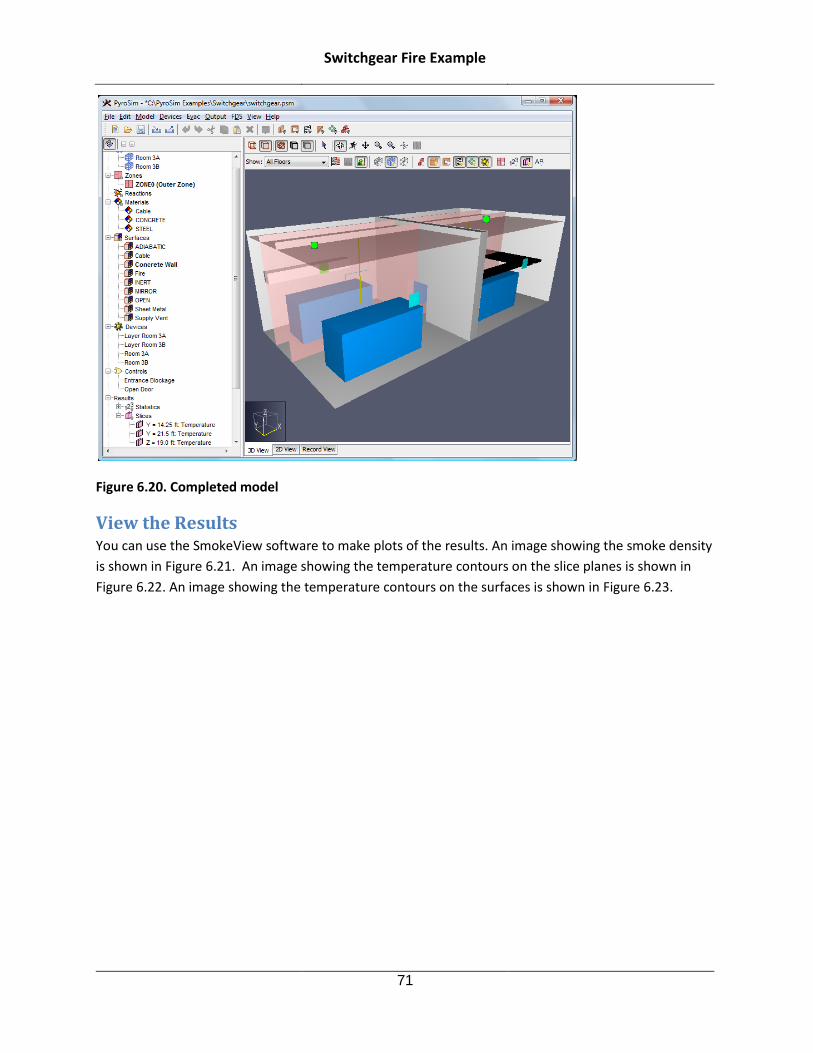
Switchgear Fire Example
71
Figure 6.20. Completed model
View the Results You can use the SmokeView software to make plots of the results. An image showing the smoke density
is shown in Figure 6.21. An image showing the temperature contours on the slice planes is shown in
Figure 6.22. An image showing the temperature contours on the surfaces is shown in Figure 6.23.

Switchgear Fire Example
72
Figure 6.21. Smoke in rooms at 100 seconds
Figure 6.22. Temperature contours on slice places at 350 seconds

Switchgear Fire Example
73
Figure 6.23. Temperature contours on the solid surfaces at 300 seconds
To view time history results
1. In the PyroSim window, on the FDS menu, click Plot Time History Results....
2. A dialog will appear showing the different types of 2D results that are available. Select
switchgear_devc.csv and click Open to view the device output. The first display will be the layer
height in Room 3A, Figure 6.24.

Switchgear Fire Example
74
Figure 6.24. Layer height in room 3A

Single Room Evacuation
75
Chapter 7. Single Room Evacuation This example walks you through a minimal FDS+EVAC example. The scenario is based on the 4th test
case in the IMO evacuation simulator verification problem list.
Figure 7.1. The EVAC example solution
Before you begin, ensure that you are using SI units (see Chapter 1).
Enable FDS+EVAC To use PyroSim’s FDS+EVAC features, these features must be manually activated. To activate PyroSim’s
FDS+EVAC features: on the Evac menu, click Enable FDS+EVAC.
Create Mesh EVAC uses a flow solution to define the movement of the occupants. This flow calculation is
independent of any meshes and flows used for the fire simulation. In this example we will use an 8 m x 5
m x 3 m EVAC mesh.
1. On the Model menu, click Edit Meshes....
2. Click New.
3. Click OK to create the new mesh.
4. In the Min X box, type 0.0 and in the Max X box, type 8.0.
5. In the Min Y box, type 0.0 and in the Max Y box, type 5.0.
6. In the Min Z box, type 0.0 and in the Max Z box, type 3.0.
7. In the X Cells box, type 16.
8. In the Y Cells box, type 10.
9. In the Z Cells box, type 1.

Single Room Evacuation
76
You can safely ignore the cell size ratio warning. All evacuation MESH records must have only 1 cell in
the Z direction.
At this point, the MESH is still a fire mesh. To specify that this mesh will be used for evacuation:
Click to select the Evacuation Mesh option.
The current setting is sufficient for MESH entries that will be used only to calculate flow fields for doors
and exits, but since this MESH will be used directly by the agents it is necessary to enable the Evac
Humans option as well:
Click to select the Evac Humans option.
See Chapter 8 of (Korhonen, et al., 2009) for a detailed discussion of the meshes.
Click OK to save changes and close the Edit Meshes dialog.
Create an Exit Each DOOR and EXIT in FDS+EVAC requires an exhaust vent to generate the correct flow field to be used
with the movement simulation. This vent must have a very weak outflow to prevent numerical
instability. We first create a surface with an exhaust flow:
1. On the Model menu, click Edit Surfaces....
2. Click New.
3. In the Surface Name type Outflow.
4. In the Surface Type list, select Exhaust.
5. Click OK to create the new surface.
6. In the Specify Velocity box, type 1.0E-6.
7. In the Ramp-Up Time list, select Tanh and in the box, type 0.1 s for the ramp-up time.
8. Click OK to close the Edit Surfaces dialog.
We now define the vent that will use the Outflow surface. To create the outflow vent:
1. On the Model menu, click New Vent....
2. In the Description type Exit Vent.
3. In the Surface list, select Outflow surface we just created.
4. Click the Geometry tab.
5. In the Plane list, select X and in the box, type 0.0 m.
6. In the Min Y box, type 1.5 and in the Max Y box, type 3.5.
7. In the Min Z box, type 0.0 and in the Max Z box, type 2.0.
8. Click the Evac tab.
9. In the Use In list, select Evac Only.
10. Click OK to close the Vent Properties dialog.

Single Room Evacuation
77
Figure 7.2. Model after adding vent
Create an EVAC exit at the same location as the Exit Vent:
1. On the Evac menu, click Exits....
2. Click New and then click OK.
3. In the Min X box, type 0.0 and in the Max X box, type 0.0.
4. In the Min Y box, type 1.5 and in the Max Y box, type 3.5.
5. In the Min Z box, type 0.0 and in the Max Z box, type 2.0.
6. In the Orientation list, select -X. This defines the direction in which the occupants will pass
through the exit.
7. Click OK to close the Edit Exits dialog.
Add Occupants Each DOOR and EXIT in FDS+EVAC requires an exhaust vent to generate the correct flow field to be used
with the movement simulation. This vent must have a very weak outflow to prevent numerical
instability. We first create a surface with an exhaust flow:
1. On the Evac menu, click Person Types....
2. Click New and click OK.
3. For the Reaction Time click the Edit button and in the x box, type 0.0. Click OK.
4. Click OK again to close the Edit PERS dialog.
To place the occupants:
1. On the Evac menu, click Initial Positions....
2. Click New and click OK.
3. In the Persons box type 50.

Single Room Evacuation
78
4. In the Min X box, type 0.0 and in the Max X box, type 8.0.
5. In the Min Y box, type 0.0 and in the Max Y box, type 5.0.
6. In the Min Z box, type 0.0 and in the Max Z box, type 2.0.
7. Click OK to close the Initial Positions dialog.
Specify Simulation Properties To define the end time:
1. On the FDS menu, click Simulation Parameters....
2. In the Simulation Title box, type Evacuation.
3. In the End Time box, type 50 s.
4. Click OK.
Save the Model This is a good time to save the model:
1. On the File menu, click Save.
2. Choose a location to save the model. Because FDS simulations generate many files and a large
amount of data, it is a good idea to use a new folder for each simulation. Name the file
evac.psm.
3. Click OK to save the model.
Run the Analysis To run the analysis:
1. On the FDS menu, click Run FDS...
View the Results The Smokeview program will launch at the end of the analysis.
1. Right-click the Smokeview window and in the Load/Unload menu select Evacuation and then
select humans.
2. Right-click the Smokeview window and in the Show/Hide menu select Use Avatar and then
select human_fixed.

Single Room Evacuation
79
Figure 7.3. Display of movement to exit
To view time history results
1. In the PyroSim window, on the FDS menu, click Plot Time History Results....
2. A dialog will appear showing a list of 2D result files. Select evac_evac.csv and click Open to view
the occupants in the room as a function of time, Figure 7.4.
Figure 7.4. Occupants as a function of time
Using Pathfinder to Solve the Same Problem Pathfinder, software developed by Thunderhead Engineering, can also perform an egress analysis. In
addition to realistic 3D images, Pathfinder can extract floors from dxf data and offers an “SFPE Mode”

Single Room Evacuation
80
that follows the SFPE Engineering Guide - Human Behavior in Fire guidelines, (SFPE, 2003). We now
repeat the same example using Pathfinder.
Figure 7.5. Snapshots of 3D movement in Pathfinder
Define the Room In Pathfinder, rooms define the geometry:
1. In the Top view, select the Add Rectangular Room tool.
2. Either click and drag or use the dimension boxes to define a room starting at X= 0.0, Y= 0.0
and extending to X= 8.0, Y= 5.0.
Create an Exit In Pathfinder, doors that do not connect rooms are exit doors. To define the door:
1. In the Top view, select the Add a New Door tool.
2. Click and drag to define a door starting at X= 0.0, Y= 1.5 and extending to X= 0.0, Y= 3.5.
Add Occupants In Pathfinder, occupants are assigned to rooms:
1. Right-click on the room and select Add Occupants....
2. By default, 50 occupants will be added. Click OK to add the occupants and close the Add
Occupants dialog.
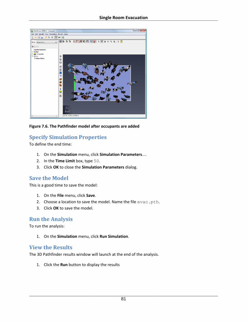
Single Room Evacuation
81
Figure 7.6. The Pathfinder model after occupants are added
Specify Simulation Properties To define the end time:
1. On the Simulation menu, click Simulation Parameters....
2. In the Time Limit box, type 50.
3. Click OK to close the Simulation Parameters dialog.
Save the Model This is a good time to save the model:
1. On the File menu, click Save.
2. Choose a location to save the model. Name the file evac.pth.
3. Click OK to save the model.
Run the Analysis To run the analysis:
1. On the Simulation menu, click Run Simulation.
View the Results The 3D Pathfinder results window will launch at the end of the analysis.
1. Click the Run button to display the results

Single Room Evacuation
82
Figure 7.7. Snapshot of 3D movement
To view time history results:
1. In the PyroSim window, on the Results menu, click Room Usage.... Note that for this analysis,
the exit times predicted by Pathfinder and FDS+EVAC are essentially identical.
Figure 7.8. Room occupants as a function of time

Example Problems Provided with FDS 5
83
Chapter 8. Example Problems Provided with FDS 5 You can import FDS 5 input files that are included with the NIST installation of FDS 5. These examples
are provided with the PyroSim distribution in the PyroSim \samples\FDS5 folder. In this chapter, we
illustrate this using a few examples; you can import additional examples. Studying these examples is a
good way to learn about input for different types of analyses.
To open any of these examples:
1. Obtain the desired FDS 5 input file.
2. Start PyroSim.
3. On the File menu, click Import and select FDS File.
4. In the Open File dialog, click the FDS input file. PyroSim will import the file. PyroSim will warn if
any records on the FDS file cannot be imported.
5. On the File menu, click Save. Save the model in a new directory.
6. On the FDS menu, click Run FDS.... This will start the analysis. At the end of the analysis,
Smokeview will be launched to view the results.
Important
If PyroSim doesn’t fully support a FDS input file, it will issue a warning that includes information about
how it handled the unfamiliar records. In some cases, PyroSim is able to add records to the Additional
Records section and the simulation is unaffected. However, if records are “dropped” (i.e. omitted from
the simulation) the simulation results will no longer represent the original intent of the example
problem.
Ethanol Pan Fire The ethanol_pan.fds example illustrates an ethanol pan fire. The model is shown in Figure 8.1. A typical
result is shown in Figure 8.2. The FDS input file can be downloaded at: http://fds-
smv.googlecode.com/svn/trunk/FDS/trunk/Validation/VU_Ethanol_Pan_Fire/FDS_Input_Files/VU_Ethan
ol_Pan_Fire.fds.

Example Problems Provided with FDS 5
84
Figure 8.1. Ethanol pan model
Figure 8.2. Ethanol pan results

Example Problems Provided with FDS 5
85
Figure 8.3. Comparison of calculated and measured heat release rates
Box Burn Away The box_burn_away.fds example illustrates burning of a foam box. The model is shown in Figure 8.4. A
typical result is shown in Figure 8.5. The FDS input file can be downloaded at: http://fds-
smv.googlecode.com/svn/trunk/FDS/trunk/Verification/Fires/box_burn_away.fds.
Figure 8.4. Foam box burn away model

Example Problems Provided with FDS 5
86
Figure 8.5. Foam box burn away results
Insulated Steel Column The insulated_steel_column.fds example illustrates heat conduction into a column. The model is shown
in Figure 8.6. A typical result is shown in Figure 8.7. The FDS input file can be downloaded at: http://fds-
smv.googlecode.com/svn/trunk/FDS/trunk/Verification/Heat_Transfer/insulated_steel_column.fds.
Figure 8.6. Insulated Steel Column model

Example Problems Provided with FDS 5
87
Figure 8.7. Insulated Steel Column results
Water Cooling The water_cooling.fds example illustrates water cooling spray onto a wall. The model is shown in Figure
8.8. A typical result is shown in Figure 8.9. The FDS input file can be downloaded at: http://fds-
smv.googlecode.com/svn/trunk/FDS/trunk/Verification/Sprinklers_and_Sprays/water_cooling.fds.
Figure 8.8. Water cooling model

Example Problems Provided with FDS 5
88
Figure 8.9. Water cooling results
Evacuation PyroSim supports input for the FDS+Evac evacuation model. The evac_example1a.fds example
illustrates evacuation from a simple room. The model is shown in Figure 8.10. A typical result is shown in
Figure 8.11. The FDS input file can be downloaded at:
http://virtual.vtt.fi/virtual/proj6/fdsevac/fds5/examples/evac_example1a.fds. For more information on
FDS+Evac, visit: http://www.vtt.fi/proj/fdsevac/index.jsp.
Please note that Thunderhead Engineering provides an agent-based evacuation model in the Pathfinder
code (http://www.thunderheadeng.com/pathfinder/index.html), which can easily import existing FDS
model geometry. The FDS+Evac and Pathfinder models can be used to provide alternate approaches to
evacuation modeling.

Example Problems Provided with FDS 5
89
Figure 8.10. Evacuation modeling example
Figure 8.11. Evacuation modeling results

References
90
References FDS-SMV Official Website. Fire Dynamics Simulator and Smokeview. Gaithersburg, Maryland, USA :
National Institute of Standards and Technology.
Klein, Bryan. 2007. Switchgear example problem, personal communication. Gaithersburg, Maryland,
USA : National Institute of Standards and Technology, 2007.
Korhonen, Time and Hostikka, Simo. 2009. Fire Dynamics Simulator with Evacuation: FDS+Evac. s.l.,
Finland : VTT Technical Research Centre of Finland, April 2009. VTT Working Papers 119.
McGrattan, Kevin and Forney, Glenn. 2005. Fire Dynamics Simulator (Version 4) User's Guide.
Washington, DC, USA : s.n., 2005. NIST Special Publication 1019.
McGrattan, Kevin. 2004. Fire Dynamics Simulator (Version 4) Technical Reference Guide. Washington,
DC, USA : s.n., 2004. NIST Special Publication 1018.
McGrattan, Kevin, et al. 2007. Fire Dynamics Simulator (Version 5) Technical Reference Guide.
Gaithersburg, Maryland, USA : s.n., October 2007. NIST Special Publication 1018-5.
McGrattan, Kevin, et al. 2007. Fire Dynamics Simulator (Version 5) User's Guide. Gaithersburg, Maryland,
USA : s.n., July 2007. NIST Special Publication 1019-5.
—. 2007. Verification and Validation of Selected Fire Models for Nuclear Power Plant Applications. s.l.,
Washington DC, USA : U.S. Nuclear Regulatory Commission, Office of Regulatory Research, May 2007.
NUREG-1824, EPRI 1011999.
SFPE. 2003. Engineering Guide - Human Behavior in Fire. Bethesda, Maryland, USA : Society of Fire
Protection Engineers, June 2003.