Pushing the Limits for Planning PatternDatabases

Stefan Edelkamp and Shahid JabbarComputer Science Department

Otto-Hahn-Str. 14University of Dortmund

April 25, 2007

Abstract

In this paper we illustrate efforts to perform memory efficient large-scale planning. We first generate sets of disjoint pattern databases space-efficiently using symbolic PDDL planning on disk. To improve the qualityof the heuristic, temporal constraints are imposed. We then apply externalmemory heuristic search and propose its integration with IDA*. Differentoptions for parallelization to save time and memory are presented. The gen-eral techniques are mapped to the (n2 − 1)-Puzzle as a running case study.

1 IntroductionHeuristic search [27] corresponds to solving an abstract problem exactly. Thisnotion of abstraction makes it possible to compute search heuristics automati-cally, opposed to domain-dependent solutions using human intuition. If abstractgoal distances are computed on-the-fly, A* can be more time-consuming thanbreadth-first search [31]. As one solution, [3] propose pattern databases (PDBs)to precompute all abstract goal distances for table look-ups in the concrete statespace.

To improve the scaling of PDBs in planning practice we integrate symbolicplanning PDBs with explicit-state external memory heuristic search. Besides thisnew combination of planning technologies, we study a number of refinements

1

to push the limits of PDBs in planning, including: control rule PDBs, sharedmemory PDBs, partitioned PDB construction, distributed PDBs. Furthermore, wepropose the integration of iterative-deepening with external memory A* search,the delayed generation of successors, and relay A* to find approximate plans. Topush the limits for these general planning techniques, we report on a large-scalecase study for the (n2 − 1)-Puzzle domain.

The paper is structured as follows. First, we introduce the case study and turnto external explicit-state A* search for solving problems that are larger than mainmemory. This solves 15-Puzzle instances optimally. We then consider planningabstractions and planning PDBs and turn to PDBs whose entries can be added.We then address different approaches for PDB compaction and introduce sym-bolic PDB based on BDDs, their construction and their addressing. We next showhow simple temporal control rules improve the quality of planning PDBs. Theintegration of IDA* to External A* search shows trade-off and optimally solvesrandom 24-Puzzle instances with one disjoint PDB. For solving the 35-Puzzle,more and larger disjoint PDBs are needed. For external symbolic PDB construc-tion, BFS-levels and sub-images are manipulated on disk. When loading differentsymbolic planning PDBs in a shared BDD, we observe additional memory gains.Subsequently we discuss and analyze the impact of a delayed generation of suc-cessors in terms of disk accesses. Furthermore, we address the distributed, space-efficient pattern lookup, which on each client selectively loads only the PDBs thatare needed to incrementally compute the heuristic estimate. This allows to loadlarger PDBs on individual processors. Last but not least, we propose relay A* togenerate approximate solution for the 35-Puzzle. Finally, we draw conclusions.

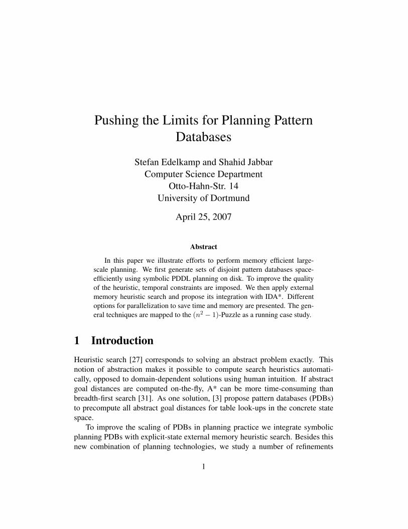
2 The (n2 − 1)-Puzzle DomainTo make our techniques explicit, we choose one specific planning benchmark,the (n2 − 1)-Puzzle. It consists of (n2 − 1) numbered tiles, squarely arranged,that can be slid into a single empty location, called the blank. The goal is tore-arrange the tiles such that a specific layout like the following ones is reached.For modeling the (n2 − 1)-puzzle every state is represented as a vector, each ofwhose components corresponds to one location, indicating by which of the tiles(including the blank) it is occupied.

2

1 2 38 47 6 5

1 2 34 5 6 78 9 10 11

12 13 14 15

1 2 3 45 6 7 8 9

10 11 12 13 1415 16 17 18 1920 21 23 23 24

1 2 3 4 56 7 8 9 10 11

12 13 14 15 16 1718 19 20 21 22 2324 25 26 27 28 2930 31 32 33 34 35

The state spaces consist of 9!/2 ≈ 1.81 · 105 states for the 8-Puzzle, 16!/2 ≈1.05 · 1013 for the 15-Puzzle, and 25!/2 ≈ 7.75 · 1024 for the 24-Puzzle, whilethe set of reachable states for the 35-Puzzle consists of 36!/2 ≈ 1.86 · 1041 states.Optimally solving the (n2 − 1)-Puzzle is NP-hard [28]. Optimal plans have beencomputed by [29] (8-Puzzle), [17] (15-Puzzle), and [22] (24-Puzzle). Approx-imate plans for the 35-Puzzle are given by [11]. A first step towards optimalsolutions is the construction of 5-tile PDBs [9].

The problem can be easily encoded in PDDL [23] with object types tileand position as well as predicates (conn ?p1 ?p2 - position) to en-code which locations are adjacent, and (on ?t - tile ?p - position)to encode on which position a tile is located. The sliding action is specified asfollows:

(:action move:parameters (?t1 - tile ?p1 ?p2 - position):precondition (and (on ?t1 ?p1)(conn ?p2 ?p1)

(forall (?t2 - tile)(not (on ?t2 ?p2)))):effect (and (not (on ?t1 ?p1))(on ?t1 ?p2)))

By its fast depth-first node generation and its linear depth space requirements,IDA* [17] is one of the best choices for solving the (n2 − 1)-Puzzle. However,IDA* comes with limited duplicate detection, which makes it less applicable toother planning domains. For improved state space coverage, different solutionshave to be found.

3 External Heuristic SearchThe limitation of main memory is the major bottleneck for practical planning ap-plications. External memory search algorithms explicitly manage the disk access,

3

since they are more informed to predict future memory accesses than the operat-ing system. It is common to measure such algorithms in the number of scans fora stream of records.

In external memory breadth-first search (BFS) the internal memory queue issubstituted with a file. Naively running internal memory BFS in the same wayon external memory results in many block file accesses for finding out whetherneighboring nodes have already been visited.

The external memory BFS graph algorithm [26] is designed for undirected ex-plicit graphs. After the preprocessing step, the graph is stored in adjacency lists.The BFS-level i− 1 is scanned and the set of successors are put into a buffer of asize close to the main memory capacity. If the buffer becomes full, internal sort-ing generates a sorted duplicate-free state sequence that is flushed. The outcomeof this phase is a file containing k partially sorted parts. Duplicate elimination isrealized (without an internal hash table) via external sorting followed by an ex-ternal scan. In the next step, external merging is applied to unify the k parts intoBFS-Level i by a simultaneous scan using k buffered file pointers. Within thisprocess duplicates are eliminated. Since the files are sorted and unless the numberof file pointers (together with their internal buffers exceed main memory), the I/Ocomplexity is determined by the time for scanning the entire file. One also has toeliminate the BFS-level i−1 and i−2 from BFS-level i to avoid re-computations.As all these levels are completely sorted, duplicates can be eliminated using aparallel scan. The process is repeated until BFS-level i becomes empty, or thegoal has been found. The correctness of restricting the duplicate scope to a con-stant number of levels builds the basis for internal sparse-memory algorithms likebreadth-first heuristic search [33], and has been extended to certain classes of di-rected graphs.

For implicit undirected problem spaces (like the 35-Puzzle) external memoryBFS has been coined to the term breadth-first frontier search with delayed dupli-cate detection [18]. The algorithm has been applied to perform a complete externalexploration of the 15-Puzzle with 1.4 terabytes hard disk in three weeks [21].

External A* [7] combines delayed duplicate detection, frontier search andbest-first enumeration to one algorithm. The organizational structure is borrowedfrom SetA* [16]. External A* maintains the search space on disk. The priorityqueue data structure to allow extracting elements with smallest f -value is a list ofbuckets. In the course of the algorithm, a bucket (i, j) contains all states s withpath length g(s) = i and the heuristic estimate h(s) = j. As same states havesame heuristic estimates, duplicate detection is restricted to buckets of the sameh-value. Each bucket is implemented as a buffered file. If a buffer becomes full,

4

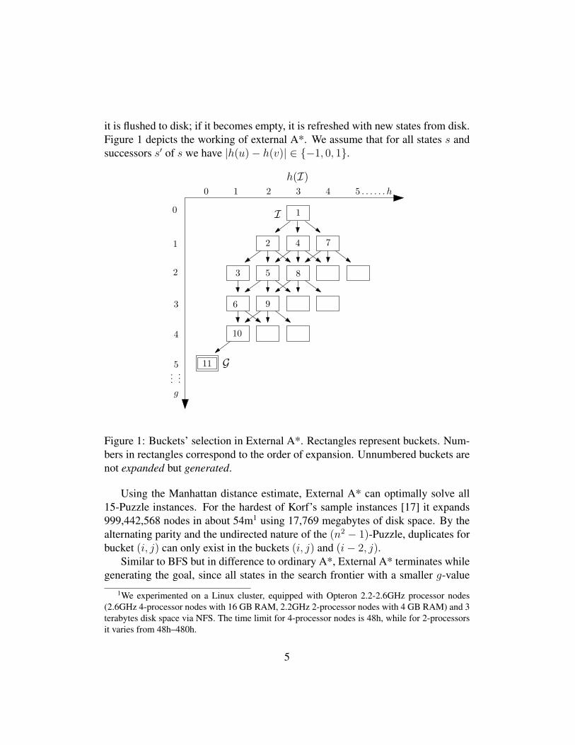
it is flushed to disk; if it becomes empty, it is refreshed with new states from disk.Figure 1 depicts the working of external A*. We assume that for all states s andsuccessors s′ of s we have |h(u) − h(v)| ∈ {−1, 0, 1}.

1

2

3

4

5

6

8

10

9

7

11

0 1 2 3 4 5 . . . . . . h

I

G

0

1

2

3

4

5...

...g

h(I)

Figure 1: Buckets’ selection in External A*. Rectangles represent buckets. Num-bers in rectangles correspond to the order of expansion. Unnumbered buckets arenot expanded but generated.

Using the Manhattan distance estimate, External A* can optimally solve all15-Puzzle instances. For the hardest of Korf’s sample instances [17] it expands999,442,568 nodes in about 54m1 using 17,769 megabytes of disk space. By thealternating parity and the undirected nature of the (n2 − 1)-Puzzle, duplicates forbucket (i, j) can only exist in the buckets (i, j) and (i − 2, j).

Similar to BFS but in difference to ordinary A*, External A* terminates whilegenerating the goal, since all states in the search frontier with a smaller g-value

1We experimented on a Linux cluster, equipped with Opteron 2.2-2.6GHz processor nodes(2.6GHz 4-processor nodes with 16 GB RAM, 2.2GHz 2-processor nodes with 4 GB RAM) and 3terabytes disk space via NFS. The time limit for 4-processor nodes is 48h, while for 2-processorsit varies from 48h–480h.

5

have already been expanded. The core problem for solving larger puzzles are goodheuristics. We will use heuristics from planning.

4 Planning Pattern DatabasesIf a state in a planning problem is described as a vector of state variables, thepattern variables denote a subset of these variables and induce an abstract space. Apattern is a specific assignment of values to the pattern variables. For the (n2−1)-Puzzle domain, a pattern reflects a particular configuration of tiles. A patterndatabase is a lookup table containing the goal distance from any abstract state. Itserves as an admissible search heuristics for the concrete state space. The size ofa PDB is the number of states it contains.

According to [4] a planning abstraction corresponds to a selection of proposi-tions as don’t cares in the grounded problem description. These are removed fromthe action in the domain description followed by a projection of the initial andgoal states. For alternative planning abstractions [15], the parameterized PDDLdomain is not changed at all. For example, abstractions simply remove domainobjects in the problem description followed by omitting atoms in the goal states.For pattern database construction, the initial state is irrelevant. For example, inthe abstraction for the (n2 − 1)-Puzzle with remaining domain objects tile-1,tile-2, tile-3, tile-4 and tile-5 the goal reduces to

(on tile-1 posn-1) (on tile-2 posn-2)(on tile-3 posn-3) (on tile-4 posn-4)(on tile-5 posn-5)

For symbolic construction, we used a PDDL planner for which input files weregenerated automatically. The selection of pattern objects is provided manually, butcan be automated [13]. Given the abstract instance, the planner finds the followingencoding for the position of each tile fully automatically.

(:group-1(on tile-1 posn-1) (on tile-1 posn-2) ...)(:group-2(on tile-2 posn-1) (on tile-2 posn-2) ...)... )

6

This representation is actually the dual of the state vector [32]. By using k bitsfor each group (k = 4 for the 15-Puzzle, 5 for the 24-Puzzle, and 6 for the 35-Puzzle), b32/kc tiles fit into one 32-bit integer, resulting in 4dn2/b32/kce bytesfor the packed state vector.

As the search space is undirected, for the construction of each PDB we se-lected forward search, starting with the abstract goal states using the original op-erators (This state space is different to backward search with inverted operators,for which many infeasible states can be generated.)

One frequently chosen option for storing the pattern databases is a perfect hashtable, which stores all goal distances in abstract space in a plain array addressedby the pattern’s hash value. It relies on a bijection of a space with n states to theset {1, . . . , n}.

5 Disjoint Planning Pattern DatabasesDisjoint planning PDBs [19] allow the addition of entries with pairwise disjointatom sets, while preserving the consistency of the estimate. As only one tilemoves at a time, for the (n2 − 1)-Puzzle the move action acts local in one group.(If an action modifies more than one group, it has to have zero costs in at least oneabstraction.)

Given a partition of the (n2 − 1)-Puzzle into tiles, disjoint PDBs can be com-puted fully automatically. Together with IDA* search, explicit-state disjoint PDBsare able to solve fully random 24-Puzzle instances [19]. Each of the PDBs in thestandard disjoint 6-tile PDBs consists of 127,512,000 abstract states (because ofthe structural regularities, out of four pattern databases only two were actuallyconstructed).

As already observed by [3], symmetries in the state vector allow multiple us-age of disjoint PDBs. For the (n2−1)-Puzzle the reflection along the main diago-nal leads to a symmetric PDB that is addressed by posing symmetric state queries.By using larger patterns explicit-state PDB grow exponentially.

6 Symbolic Planning Pattern DatabasesCompressed PDBs [10] can be constructed either by compiling the database pos-terior to its construction, or on-the-fly during the construction process [8]. More-over, one can approximate the PDB content, by hash table folding [20].

7

Trie PDBs [30] (commonly used for storing patters in the multiple sequencealignment problem) are compact PDBs that allow sharing of state vectors. Eachpath from the root to a leaf corresponds to a complete scan of the state vector.Tries are either multi-variate (each branch corresponds to a state vector entry offinite domain, e.g., the tiles’ label) or binary (each path corresponds to the binaryrepresentation of the state vector). They can be compressed by contracting edgesthat contain no branching.

Symbolic PDBs [5] are compact representations of trie PDBs on binary statevectors. The functional representation of state set is a binary decision diagram(BDD) [2]. For a given state vector, the BDD evaluates to 1, if the correspondingstate is contained in the encoded set. The additional compaction refers to the twoBDD reduction rule, which lead to a unique diagram representation. In terms ofBDDs, a symbolic PDB can be seen as a sequence of BDDs PDB1, . . . , PDBk

with PDBi covering the state vector representations of all abstract states that havea h-value of i.

The symbolic construction of the standard disjoint 6-tile PDB for the 24-Puzzle (in about half an hour each) lead to PDB of 96,352,162 and 95,766,454bytes (≈ 30% savings).

In theory, the lookup in a symbolic PBDs can be faster than in a hash table,as not all state variables have to be looked at to determine, whether or not a stateis contained in it. In practice, however, the retrieval in symbolic PDBs is oftenslower due to changing the encoding, transforming numbers into binary, callinginterfaces to BDD libraries, a worse cache reputation. For external search theevaluation is sufficiently fast compared to manipulating states on disk.

Instead of compacting the explicit-state PDB, the construction process of theabstract state space itself is symbolic with the abstract goal and all abstract op-erators represented in form of a BDD. The abstract operators represent transitionrelation in partitioned form and are used to compute the one-step image of a stateset [24].

7 Pattern Database Control RulesTemporal constraints have been recently added to PDDL [12]. The constraint(hold-during t1 t2 φ) requires φ to be true in step t1 ≤ i < t2. Such con-straints map to timed initial literals as introduced by [14].

Using temporal constraints, the quality of PDBs can be improved. Consider aPDB for the sliding-tile puzzle with a set of pattern tiles that surround the blank

8

in the top-left corner. We know that the last action necessarily has to move a tilethat is adjacent to the blank. In the 35-Puzzle these are the tile-1 and tile-5.When constructing the PDB that includes these two tiles in the pattern (startingwith the goal) we simply add the following constraint to the PDDL encoding.

(hold-during 1 2 (or (on tile-1 posn-0)(on tile-5 posn-0)))

The second last move may also have restrictions. Suppose that tile-10 andtile-6 are also contained in the pattern for the PDB. Then

(hold-during 2 3 (or (on tile-1 posn-0)(or (on tile-10 posn-6)

(on tile-6 posn-6))))

There are some subtleties. First, temporal constraints may transform undi-rected search spaces to a directed ones, implying an increase of the duplicate de-tection scope (needed for frontier search construction). Secondly, the PDBs mayloose consistency as successors in concrete space may not be in adjacent levels inthe abstract space. As such successors produce sub-optimal solution, such statescan safely be omitted from the search.

In planning practice, the integration of these control rules leads to an increaseof radius 32 to radius 35 for the irregular 6-tile pattern database of the 24-Puzzle.We use these improved PDBs for the 24-Puzzle experiments.

8 Incremental External SearchWhile External A* requires a constant amount of memory due to internal read andwrite buffers for the files, IDA* requires memory that scales linear with the searchdepth. External A* removes all duplicates from the search but require slow diskto succeed. Moreover, in search practice disk space is limited, too.

Therefore, one may wish to combine advantages of IDA* and External A*.First of all, simple pruning strategies such as not generating predecessor statesagain, help to save external work for delayed duplicate detection. Moreover, aswe will see, incremental heuristics (the successor’s h-value is computed by theold h-value and the heuristic difference) stored together with the state acceleratesPDB lookup time.

9

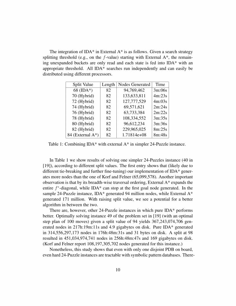
The integration of IDA* in External A* is as follows. Given a search strategysplitting threshold (e.g., on the f -value) starting with External A*, the remain-ing unexpanded buckets are only read and each state is fed into IDA* with anappropriate threshold. All IDA* searches run independently and can easily bedistributed using different processors.

Split Value Length Nodes Generated Time68 (IDA*) 82 94,769,462 3m:06s

70 (Hybrid) 82 133,633,811 4m:23s72 (Hybrid) 82 127,777,529 4m:03s74 (Hybrid) 82 69,571,621 2m:24s76 (Hybrid) 82 63,733,384 2m:22s78 (Hybrid) 82 108,334,552 3m:35s80 (Hybrid) 82 96,612,234 3m:36s82 (Hybrid) 82 229,965,025 8m:25s

84 (External A*) 82 1.71814e+08 8m:48s

Table 1: Combining IDA* with external A* in simpler 24-Puzzle instance.

In Table 1 we show results of solving one simpler 24-Puzzles instance (40 in[19]), according to different split values. The first entry shows that (likely due todifferent tie-breaking and further fine-tuning) our implementation of IDA* gener-ates more nodes than the one of Korf and Felner (65,099,578). Another importantobservation is that by its breadth-wise traversal ordering, External A* expands theentire f ∗-diagonal, while IDA* can stop at the first goal node generated. In thesample 24-Puzzle instance, IDA* generated 94 million nodes, while External A*generated 171 million. With raising split value, we see a potential for a betteralgorithm in between the two.

There are, however, other 24-Puzzle instances in which pure IDA* performsbetter. Optimally solving instance 49 of the problem set in [19] (with an optimalstep plan of 100 moves) given a split value of 94 yields 367,243,074,706 gen-erated nodes in 217h:19m:11s and 4.9 gigabytes on disk. Pure IDA* generatedin 314,556,297,173 nodes in 176h:48m:31s and 31 bytes on disk. A split at 98resulted in 451,034,974,741 nodes in 256h:48m:47s and 169 gigabytes on disk.(Korf and Felner report 108,197,305,702 nodes generated for this instance.)

Nonetheless, this study shows that even with only one disjoint PDB on board,even hard 24-Puzzle instances are tractable with symbolic pattern databases. There-

10

fore, in the following we concentrate on scaling the number and size of planningPDBs for solving the 35-Puzzle.

With x tiles in the pattern, the abstract state space for the 35-Puzzle consistsof 36!/(36 − x)! states. For x = 1 a PDB stores the Manhattan distances for theselected tile, inducing an abstract state space consisting of 36 states. The sizes forlarger values of x are: 36!/34! ≈ 1.26 · 103 (x = 2), 36!/33! ≈ 4.28 · 104 (x = 3),36!/32! ≈ 1.41 · 106 (x = 4), 36!/31! ≈ 4.52 · 107 (x = 5), 36!/30! ≈ 1.40 · 109

(x = 6), and 36!/29! ≈ 4.2 · 1010 (x = 7). Assuming one byte per entry, aperfect hash-based PDB for the 35-Puzzle calls for about 1.23 kilobytes (x = 2),41.83 kilobytes (x = 3), 1.34 megabytes (x = 4), 43.14 megabytes (x = 5), 1.3gigabytes (x = 6), and 39.1 gigabytes (x = 7) RAM. Note that for generating theabstract state space, the search frontier additionally has to be stored, but to keepthe comparison simple, we assume this frontier to be maintained on disk.

9 External Planning Pattern DatabasesExternal PDBs [6] are constructed in layers and maintained on the hard disk. EachBFS level is flushed in form of a BDD to disk, so that the memory for representingthis level can be re-used. As the BDD representation of a state set is unique, noeffort for eliminating duplicates in one BFS-level is required. Before expandinga state set, however, we apply delayed duplicate detection wrt. the set of the twoprevious BFS-levels. As the external construction of large-scale PDBs may takelong, the process can be paused and resumed at any time.

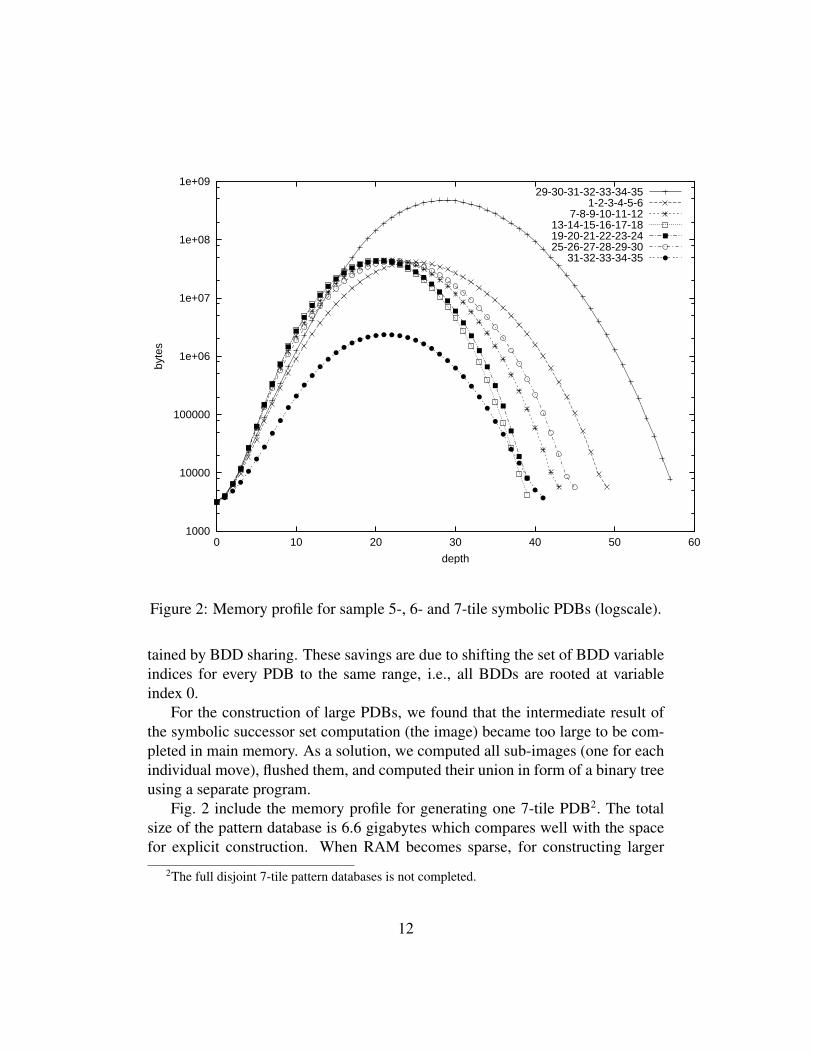
For the 35-Puzzle either seven 5-tile, five 6-tile and one 5-tile, or five 7-tile databases complete a disjoint set. The cumulated space consumption forexplicit-state disjoint sets of PDBs (without exploiting structural regularities) is302 megabytes (for x = 5), 6.9 gigabytes (for x = 6), and 195 gigabytes (forx = 7). For the disjoint 6-tile PDB in the 35-Puzzle the results are shown inFig. 2. In total the additive set consumes 2.6 gigabytes; a gain of factor 2.65 wrt.the explicit construction. We generated four more additive 6-tile PDBs with sizes4.0, 2.3, 2.3, and 3.2 gigabytes. The construction of all five disjoint 6-tile PDBstook about 50h.

Together with the space of about one gigabyte for the search buckets (5 · 106

entries), one would expect a main memory requirement of more than 15 gigabyteswhen loading all 5 disjoint PDBs. However, about 13 gigabytes RAM were ac-tually neede. This additional memory gain is due to loading the different layersstored on disk into a shared BDD [25]. There are also cross-PDB savings, ob-

11

1000

10000

100000

1e+06

1e+07

1e+08

1e+09

0 10 20 30 40 50 60

byte

s

depth

29-30-31-32-33-34-351-2-3-4-5-6

7-8-9-10-11-1213-14-15-16-17-1819-20-21-22-23-2425-26-27-28-29-30

31-32-33-34-35

Figure 2: Memory profile for sample 5-, 6- and 7-tile symbolic PDBs (logscale).

tained by BDD sharing. These savings are due to shifting the set of BDD variableindices for every PDB to the same range, i.e., all BDDs are rooted at variableindex 0.

For the construction of large PDBs, we found that the intermediate result ofthe symbolic successor set computation (the image) became too large to be com-pleted in main memory. As a solution, we computed all sub-images (one for eachindividual move), flushed them, and computed their union in form of a binary treeusing a separate program.

Fig. 2 include the memory profile for generating one 7-tile PDB2. The totalsize of the pattern database is 6.6 gigabytes which compares well with the spacefor explicit construction. When RAM becomes sparse, for constructing larger

2The full disjoint 7-tile pattern databases is not completed.

12

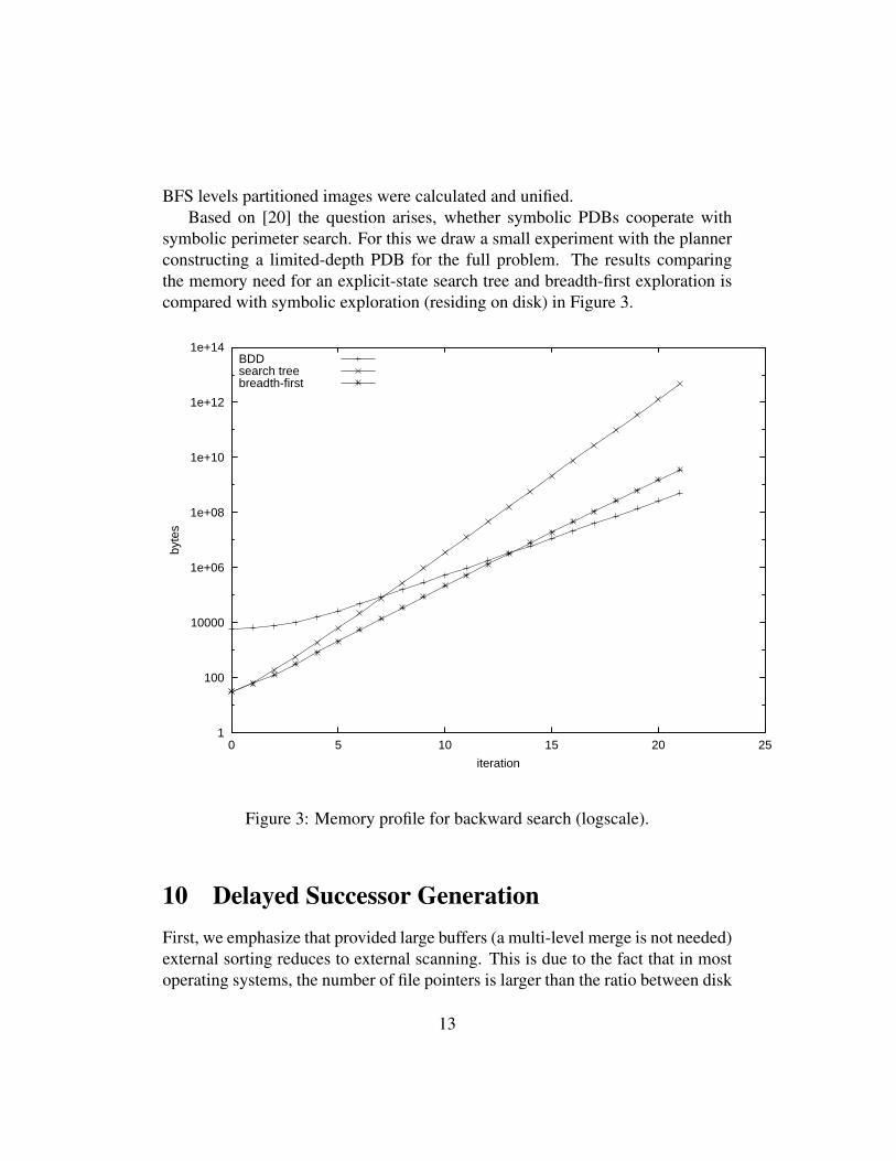
BFS levels partitioned images were calculated and unified.Based on [20] the question arises, whether symbolic PDBs cooperate with

symbolic perimeter search. For this we draw a small experiment with the plannerconstructing a limited-depth PDB for the full problem. The results comparingthe memory need for an explicit-state search tree and breadth-first exploration iscompared with symbolic exploration (residing on disk) in Figure 3.

1

100

10000

1e+06

1e+08

1e+10

1e+12

1e+14

0 5 10 15 20 25

byte

s

iteration

BDDsearch treebreadth-first

Figure 3: Memory profile for backward search (logscale).

10 Delayed Successor GenerationFirst, we emphasize that provided large buffers (a multi-level merge is not needed)external sorting reduces to external scanning. This is due to the fact that in mostoperating systems, the number of file pointers is larger than the ratio between disk

13

and main memory and can also be increased by recompiling the kernel. Given thata single merging pass suffices, the I/O complexity is bounded by O(|E|/B), withE = {(s, s′) | s′ is successor of s ∧ f(s) ≤ f ∗} and B being the block size.

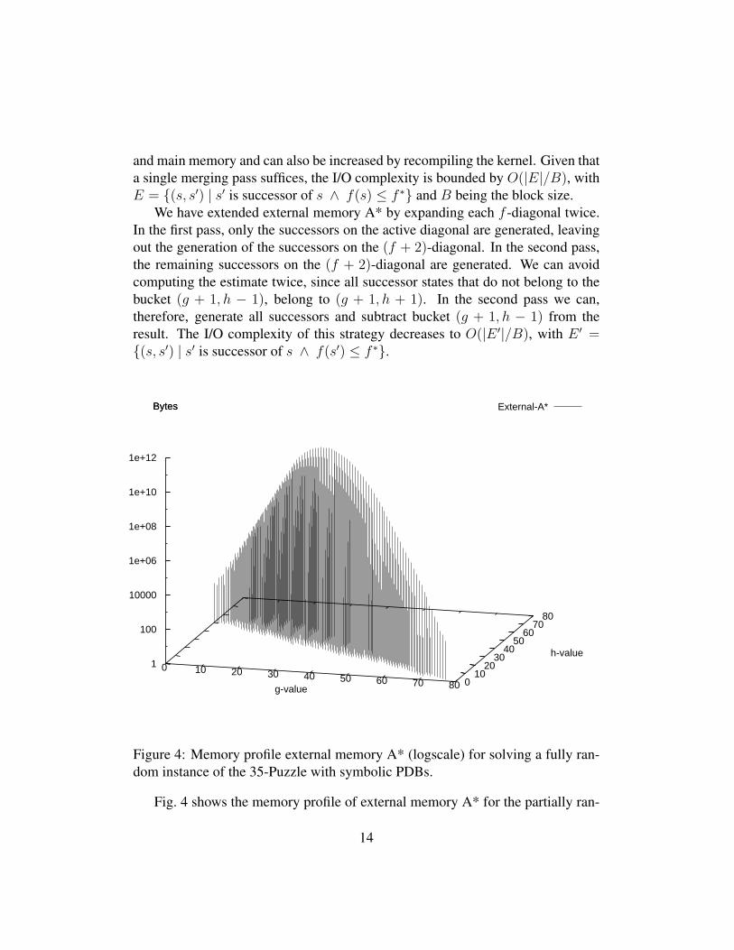
We have extended external memory A* by expanding each f -diagonal twice.In the first pass, only the successors on the active diagonal are generated, leavingout the generation of the successors on the (f + 2)-diagonal. In the second pass,the remaining successors on the (f + 2)-diagonal are generated. We can avoidcomputing the estimate twice, since all successor states that do not belong to thebucket (g + 1, h − 1), belong to (g + 1, h + 1). In the second pass we can,therefore, generate all successors and subtract bucket (g + 1, h − 1) from theresult. The I/O complexity of this strategy decreases to O(|E ′|/B), with E ′ ={(s, s′) | s′ is successor of s ∧ f(s′) ≤ f ∗}.

0 10 20 30 40 50 60 70 80 0 10

20 30

40 50

60 70

80

1

100

10000

1e+06

1e+08

1e+10

1e+12

Bytes External-A*

g-value

h-value

Bytes

Figure 4: Memory profile external memory A* (logscale) for solving a fully ran-dom instance of the 35-Puzzle with symbolic PDBs.

Fig. 4 shows the memory profile of external memory A* for the partially ran-

14

CPU Time Total Time RAM12h:32m:20s 48h:00m:10s 4,960,976 kilobytes

9h:55m:59s 48h:00m:25s 4,960,980 kilobytes8h:35m:43s 45h:33m:02s 4,960,976 kilobytes8h:45m:53s 39h:36m:22s 4,960,988 kilobytes

10h:25m:31s 46h:31m:35s 4,960,976 kilobytes11h:38m:36s 48h:00m:40s 4,960,988 kilobytes8h:04m:14s 26h:37m:30s 4,960,984 kilobytes

66h:58m:16s 302h:19m:44s

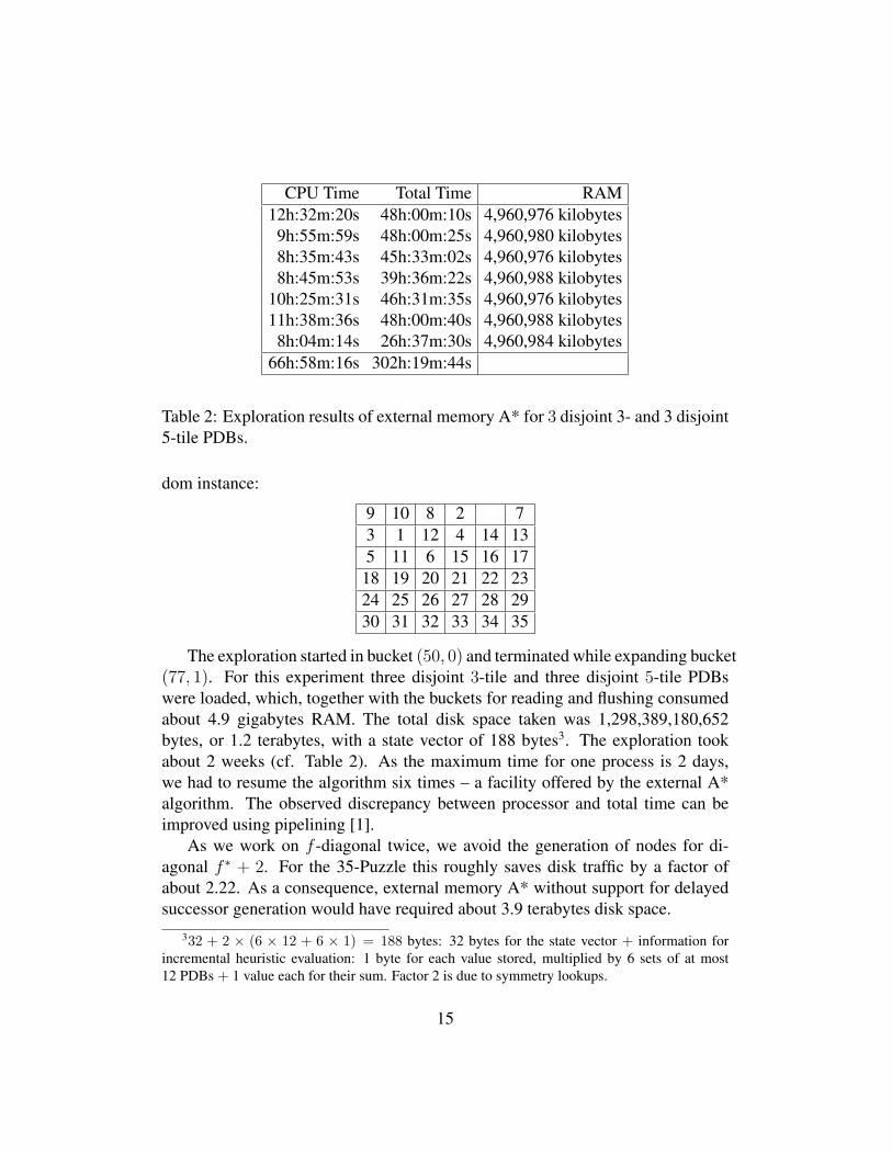
Table 2: Exploration results of external memory A* for 3 disjoint 3- and 3 disjoint5-tile PDBs.

dom instance:

9 10 8 2 73 1 12 4 14 135 11 6 15 16 17

18 19 20 21 22 2324 25 26 27 28 2930 31 32 33 34 35

The exploration started in bucket (50, 0) and terminated while expanding bucket(77, 1). For this experiment three disjoint 3-tile and three disjoint 5-tile PDBswere loaded, which, together with the buckets for reading and flushing consumedabout 4.9 gigabytes RAM. The total disk space taken was 1,298,389,180,652bytes, or 1.2 terabytes, with a state vector of 188 bytes3. The exploration tookabout 2 weeks (cf. Table 2). As the maximum time for one process is 2 days,we had to resume the algorithm six times – a facility offered by the external A*algorithm. The observed discrepancy between processor and total time can beimproved using pipelining [1].

As we work on f -diagonal twice, we avoid the generation of nodes for di-agonal f ∗ + 2. For the 35-Puzzle this roughly saves disk traffic by a factor ofabout 2.22. As a consequence, external memory A* without support for delayedsuccessor generation would have required about 3.9 terabytes disk space.

332 + 2 × (6 × 12 + 6 × 1) = 188 bytes: 32 bytes for the state vector + information forincremental heuristic evaluation: 1 byte for each value stored, multiplied by 6 sets of at most12 PDBs + 1 value each for their sum. Factor 2 is due to symmetry lookups.

15

CPU Time Total Time RAM20h:57m:43s 48h:00m:35s 13,164,060 kilobytes2h:18m:47s 5h:08m:44s 13,164,068 kilobytes

18h:28m:38s 42h:23m:08s 13,164,064 kilobytes22h:55m:48s 45h:33m:47s 13,164,068 kilobytes12h:38m:31s 24h:16m:32s 13,164,068 kilobytes77h:19m:27s 165h:22m:46s

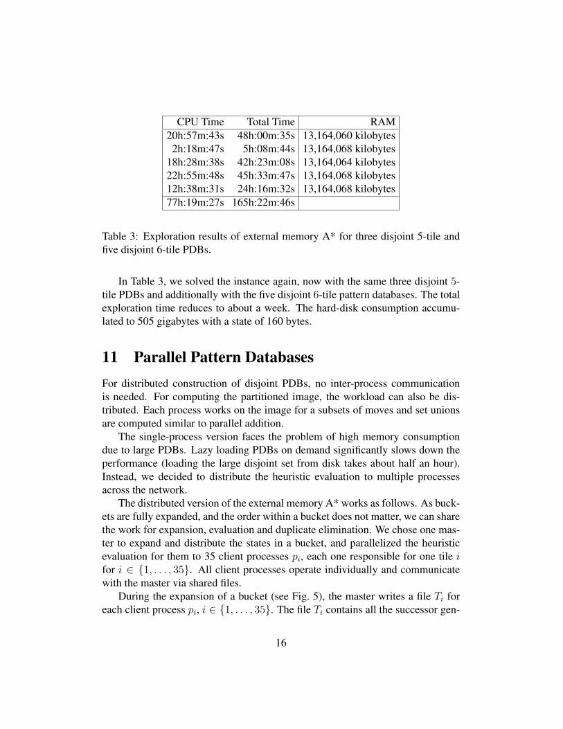
Table 3: Exploration results of external memory A* for three disjoint 5-tile andfive disjoint 6-tile PDBs.

In Table 3, we solved the instance again, now with the same three disjoint 5-tile PDBs and additionally with the five disjoint 6-tile pattern databases. The totalexploration time reduces to about a week. The hard-disk consumption accumu-lated to 505 gigabytes with a state of 160 bytes.

11 Parallel Pattern DatabasesFor distributed construction of disjoint PDBs, no inter-process communicationis needed. For computing the partitioned image, the workload can also be dis-tributed. Each process works on the image for a subsets of moves and set unionsare computed similar to parallel addition.

The single-process version faces the problem of high memory consumptiondue to large PDBs. Lazy loading PDBs on demand significantly slows down theperformance (loading the large disjoint set from disk takes about half an hour).Instead, we decided to distribute the heuristic evaluation to multiple processesacross the network.

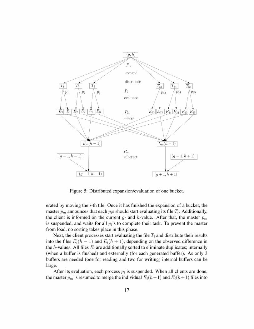
The distributed version of the external memory A* works as follows. As buck-ets are fully expanded, and the order within a bucket does not matter, we can sharethe work for expansion, evaluation and duplicate elimination. We chose one mas-ter to expand and distribute the states in a bucket, and parallelized the heuristicevaluation for them to 35 client processes pi, each one responsible for one tile ifor i ∈ {1, . . . , 35}. All client processes operate individually and communicatewith the master via shared files.

During the expansion of a bucket (see Fig. 5), the master writes a file Ti foreach client process pi, i ∈ {1, . . . , 35}. The file Ti contains all the successor gen-

16

Pm

p1 p3

Pm

p34 p35p33

T1 T2 T3 T33 T34

p2

T35

E1 E2 E3 E33 E34 E35

(g, h)

(g + 1, h− 1)

distribute

merge

evaluate

subtract

expand

Em(h− 1)

(g + 1, h + 1)

Em(h + 1)

E1 E2 E3 E33 E34 E35

Pm

Pi

(g − 1, h− 1) (g − 1, h + 1)

Figure 5: Distributed expansion/evaluation of one bucket.

erated by moving the i-th tile. Once it has finished the expansion of a bucket, themaster pm announces that each pis should start evaluating its file Ti. Additionally,the client is informed on the current g- and h-value. After that, the master pm

is suspended, and waits for all pi’s to complete their task. To prevent the masterfrom load, no sorting takes place in this phase.

Next, the client processes start evaluating the file Ti and distribute their resultsinto the files Ei(h − 1) and Ei(h + 1), depending on the observed difference inthe h-values. All files Ei are additionally sorted to eliminate duplicates; internally(when a buffer is flushed) and externally (for each generated buffer). As only 3buffers are needed (one for reading and two for writing) internal buffers can belarge.

After its evaluation, each process pi is suspended. When all clients are done,the master pm is resumed to merge the individual Ei(h−1) and Ei(h+1) files into

17

Em(h− 1) and Em(h+1). The merging preserves the order in the files Ei(h− 1)and Ei(h + 1), so that the files Em(h − 1) and Em(h + 1) are sorted with allbucket duplicates eliminated. The subtraction of the bucket (g − 1, h − 1) fromEm(h− 1) and (g− 1, h+1) from Em(h+1) now eliminates duplicates from thesearch using a parallel scan of both files4.

7-tiles additive PDB

D1 D2 D3D1 D2 D3 D4

p1 p2 p3 p33 p34 p35

6-tiles additive PDBs

D1 D2 D3D2 D3 D4

p1 p2 p3 p33 p34 p35

D0 D5 D0 D4

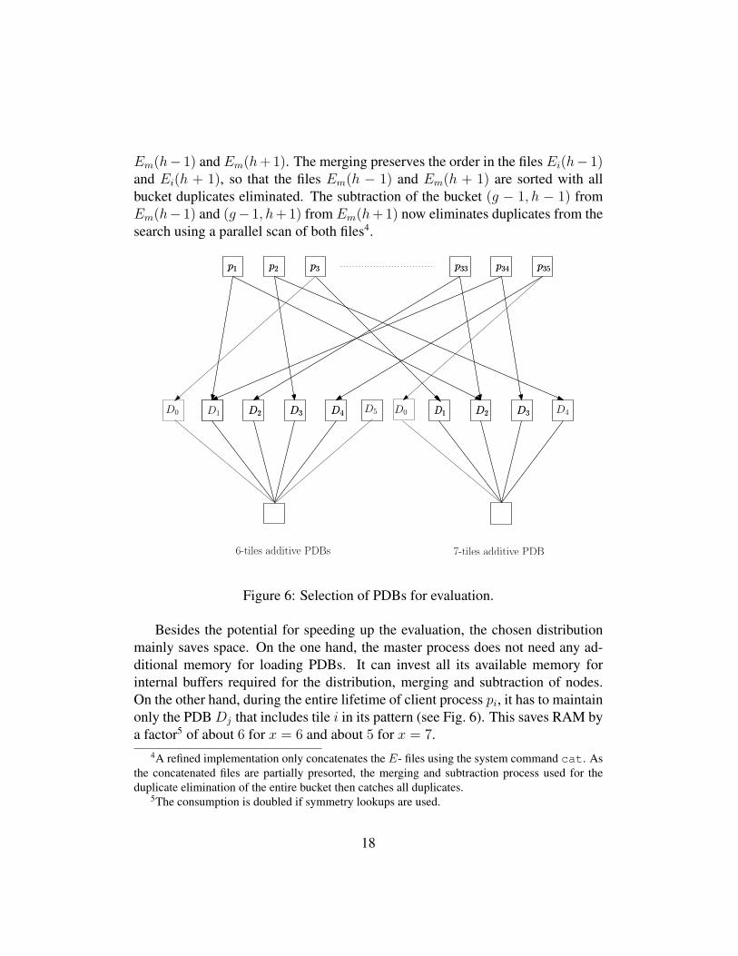
Figure 6: Selection of PDBs for evaluation.

Besides the potential for speeding up the evaluation, the chosen distributionmainly saves space. On the one hand, the master process does not need any ad-ditional memory for loading PDBs. It can invest all its available memory forinternal buffers required for the distribution, merging and subtraction of nodes.On the other hand, during the entire lifetime of client process pi, it has to maintainonly the PDB Dj that includes tile i in its pattern (see Fig. 6). This saves RAM bya factor5 of about 6 for x = 6 and about 5 for x = 7.

4A refined implementation only concatenates the E- files using the system command cat. Asthe concatenated files are partially presorted, the merging and subtraction process used for theduplicate elimination of the entire bucket then catches all duplicates.

5The consumption is doubled if symmetry lookups are used.

18

We started two parallel external memory A* explorations for solving the halfinstances using 35 clients and one master process. The individual RAM require-ments for the clients reduced to 1.3 gigabytes so that 2 processes could be runon one node. This proves that a considerable amount of RAM can be saved on anode using parallel execution - the most critical resource for the exploration withplanning PDBs. The first exploration (first 17 tiles permuted) took 3h:34m and4.3 gigabytes to complete, while the second exploration (last 18 tiles permuted)took 4h:29m and 19 gigabytes.

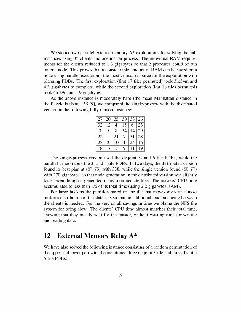
As the above instance is moderately hard (the mean Manhattan distance inthe Puzzle is about 135 [9]) we compared the single-process with the distributedversion in the following fully random instance:

27 20 35 30 33 2632 12 4 15 6 233 5 8 34 14 29

22 21 7 31 2825 2 10 1 24 1618 17 13 9 11 19

The single-process version used the disjoint 5- and 6 tile PDBs, while theparallel version took the 3- and 5-tile PDBs. In two days, the distributed versionfound its best plan at (87, 75) with 338, while the single version found (85, 77)with 270 gigabytes, so that node generation in the distributed version was slightlyfaster even though it generated many intermediate files. The masters’ CPU timeaccumulated to less than 1/6 of its total time (using 2.2 gigabytes RAM).

For large buckets the partition based on the tile that moves gives an almostuniform distribution of the state sets so that no additional load balancing betweenthe clients is needed. For the very small savings in time we blame the NFS filesystem for being slow. The clients’ CPU time almost matches their total time,showing that they mostly wait for the master, without wasting time for writingand reading data.

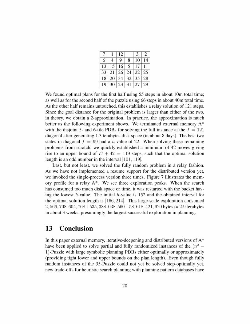
12 External Memory Relay A*We have also solved the following instance consisting of a random permutation ofthe upper and lower part with the mentioned three disjoint 3-tile and three disjoint5-tile PDBs:

19

7 1 12 3 26 4 9 8 10 14

13 15 16 5 17 1133 21 26 24 22 2518 20 34 32 35 2819 30 23 31 27 29

We found optimal plans for the first half using 55 steps in about 10m total time;as well as for the second half of the puzzle using 66 steps in about 40m total time.As the other half remains untouched, this establishes a relay solution of 121 steps.Since the goal distance for the original problem is larger than either of the two,in theory, we obtain a 2-approximation. In practice, the approximation is muchbetter as the following experiment shows. We terminated external memory A*with the disjoint 5- and 6-tile PDBs for solving the full instance at the f = 121diagonal after generating 1.3 terabytes disk space (in about 8 days). The best twostates in diagonal f = 99 had a h-value of 22. When solving these remainingproblems from scratch, we quickly established a minimum of 42 moves givingrise to an upper bound of 77 + 42 = 119 steps, such that the optimal solutionlength is an odd number in the interval [101, 119].

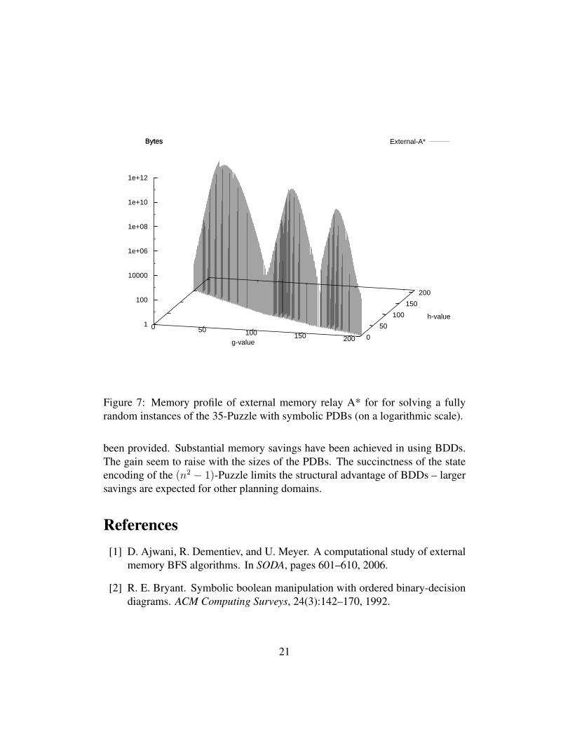
Last, but not least, we solved the fully random problem in a relay fashion.As we have not implemented a resume support for the distributed version yet,we invoked the single-process version three times. Figure 7 illustrates the mem-ory profile for a relay A*. We see three exploration peaks. When the searchhas consumed too much disk space or time, it was restarted with the bucket hav-ing the lowest h-value. The initial h-value is 152 and the obtained interval forthe optimal solution length is [166, 214]. This large-scale exploration consumed2, 566, 708, 604, 768+535, 388, 038, 560+58, 618, 421, 920 bytes ≈ 2.9 terabytesin about 3 weeks, presumingly the largest successful exploration in planning.

13 ConclusionIn this paper external memory, iterative-deepening and distributed versions of A*have been applied to solve partial and fully randomized instances of the (n2 −1)-Puzzle with large symbolic planning PDBs either optimally or approximately(providing tight lower and upper bounds on the plan length). Even though fullyrandom instances of the 35-Puzzle could not yet be solved step-optimally yet,new trade-offs for heuristic search planning with planning pattern databases have

20

0 50 100 150 200 0

50

100

150

200

1

100

10000

1e+06

1e+08

1e+10

1e+12

Bytes External-A*

g-value

h-value

Bytes

Figure 7: Memory profile of external memory relay A* for for solving a fullyrandom instances of the 35-Puzzle with symbolic PDBs (on a logarithmic scale).

been provided. Substantial memory savings have been achieved in using BDDs.The gain seem to raise with the sizes of the PDBs. The succinctness of the stateencoding of the (n2 − 1)-Puzzle limits the structural advantage of BDDs – largersavings are expected for other planning domains.

References[1] D. Ajwani, R. Dementiev, and U. Meyer. A computational study of external

memory BFS algorithms. In SODA, pages 601–610, 2006.

[2] R. E. Bryant. Symbolic boolean manipulation with ordered binary-decisiondiagrams. ACM Computing Surveys, 24(3):142–170, 1992.

21

[3] J. C. Culberson and J. Schaeffer. Pattern databases. Computational Intelli-gence, 14(4):318–334, 1998.

[4] S. Edelkamp. Planning with pattern databases. In European Conference onPlanning (ECP), pages 13–24, 2001.

[5] S. Edelkamp. Symbolic pattern databases in heuristic search planning. InAIPS, pages 274–293, 2002.

[6] S. Edelkamp. External symbolic heuristic search with pattern databases. InICAPS, pages 51–60, 2005.

[7] S. Edelkamp, S. Jabbar, and S. Schrodl. External A*. In German Conferenceon Artificial Intelligence (KI), pages 233–250, 2004.

[8] A. Felner and A. Alder. Solving the 24 puzzle with instance dependentpattern databases. In SARA, pages 248–260, 2005.

[9] A. Felner, R. Korf, and S. Hanan. Additive pattern databases. Journal ofArtificial Intelligence Research, 22:279–318, 2004.

[10] A. Felner, R. Meshulam, R. C. Holte, and R. E. Korf. Compressing patterndatabases. In AAAI, pages 638–643, 2004.

[11] D. Furcy and S. Koenig. Scaling up WA* with commitment and diversity.In IJCAI, pages 1521–1522, 2005.

[12] A. Gerevini and D. Long. Plan constraints and preferences in PDDL3. Tech-nical report, Department of Electronics for Automation, University of Bres-cia, 2005.

[13] P. Haslum. Domain-independent construction of pattern database heuristicsfor cost-optimal planning, 2007. Personal communications.

[14] J. Hoffmann and S. Edelkamp. The deterministic part of IPC-4: Anoverview. Journal of Artificial Intelligence Research, 24:519–579, 2005.

[15] J. Hoffmann, A. Sabharwal, and C. Domshlak. Friends or foes? An AIplanning perspective on abstraction and search. pages 294–304, 2006.

[16] R. M. Jensen, R. E. Bryant, and M. M. Veloso. SetA*: An efficient BDD-based heuristic search algorithm. In AAAI, pages 668–673, 2002.

22

[17] R. E. Korf. Depth-first iterative-deepening: An optimal admissible treesearch. Artificial Intelligence, 27(1):97–109, 1985.

[18] R. E. Korf. Breadth-first frontier search with delayed duplicate detection. InMOCHART, pages 87–92, 2003.

[19] R. E. Korf and A. Felner. Chips Challenging Champions: Games, Comput-ers and Artificial Intelligence, chapter Disjoint Pattern Database Heuristics,pages 13–26. Elsevier, 2002.

[20] R. E. Korf and A. Felner. Recent progress in heuristic search: A case studyof the four-peg towers of hanoi problem. In IJCAI, pages 2324–2329, 2007.

[21] R. E. Korf and T. Schultze. Large-scale parallel breadth-first search. InAAAI, pages 1380–1385, 2005.

[22] R. E. Korf and L. A. Taylor. Finding optimal solutions to the twenty-fourpuzzle. In AAAI, pages 1202–1207, 1996.

[23] D. McDermott. The 1998 AI Planning Competition. AI Magazine, 21(2),2000.

[24] K. McMillan. Symbolic Model Checking. Kluwer Academic Press, 1993.

[25] S. Minato, N. Ishiura, and S. Yajima. Shared binary decision diragram withattributed edges for efficient boolean function manipuation. In Design Au-tomation Conference (DAC), pages 52–57, 1990.

[26] K. Munagala and A. Ranade. I/O-complexity of graph algorithms. In Sym-posium on Discrete Algorithms, pages 687–694, 1999.

[27] J. Pearl. Heuristics. Addison-Wesley, 1985.

[28] D. Ratner and M. K. Warmuth. The (n2 − 1)-puzzle and related relocationproblems. Journal of Symbolic Computation, 10(2):111–137, 1990.

[29] P. D. A. Schofield. Complete solution of the eight puzzle. In Machine Intel-ligence 2, pages 125–133. Elsevier, 1967.

[30] S. Schroedl. An improved search algorithm for optimal multiple sequencealignment. Journal of Artificial Intelligence Research, 23:587–623, 2005.

23

[31] M. Valtorta. A result on the computational complexity of heuristic estimatesfor the A* algorithm. Information Sciences, 34:48–59, 1984.

[32] U. Zahavi, A. Felner, R. Holte, and J. Schaeffer. Dual search in permutationstate spaces. In AAAI, pages 1076–1081, 2006.

[33] R. Zhou and E. A. Hansen. Breadth-first heuristic search. Artificial Intelli-gence, 170(4-5):385–408, 2006.

24