Push Vs. Pull Part Two – Focus on MRP

IE 3265 POM

R. R. Lindeke, Ph. D.

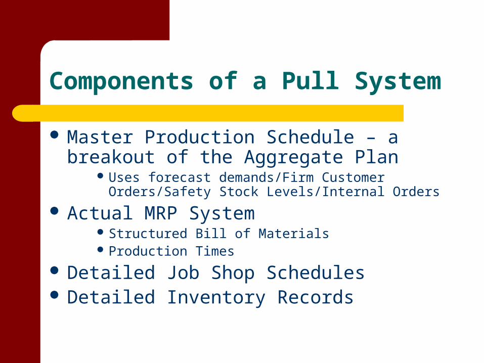
Components of a Pull System

Master Production Schedule – a breakout of the Aggregate Plan

Uses forecast demands/Firm Customer Orders/Safety Stock Levels/Internal Orders

Actual MRP System Structured Bill of Materials Production Times

Detailed Job Shop Schedules Detailed Inventory Records

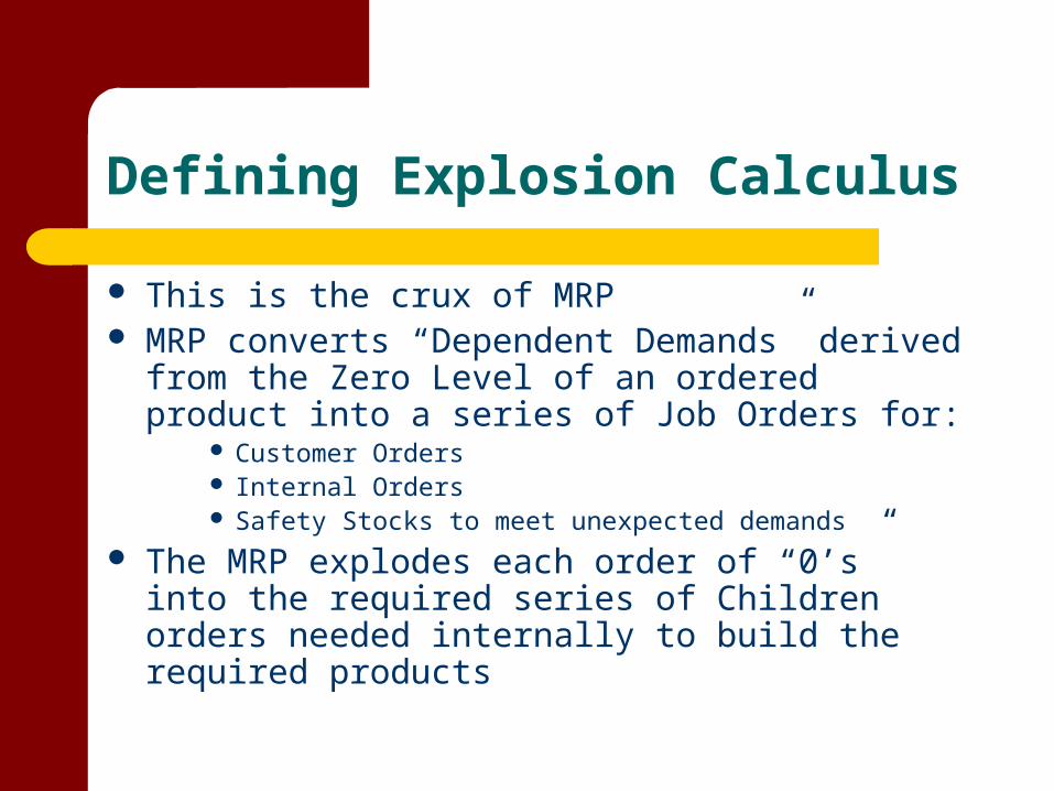
Defining Explosion Calculus

This is the crux of MRP MRP converts “Dependent Demands” derived from

the Zero Level of an ordered product into a series of Job Orders for:

Customer Orders Internal Orders Safety Stocks to meet unexpected demands

The MRP explodes each order of “0’s” into the required series of Children orders needed internally to build the required products

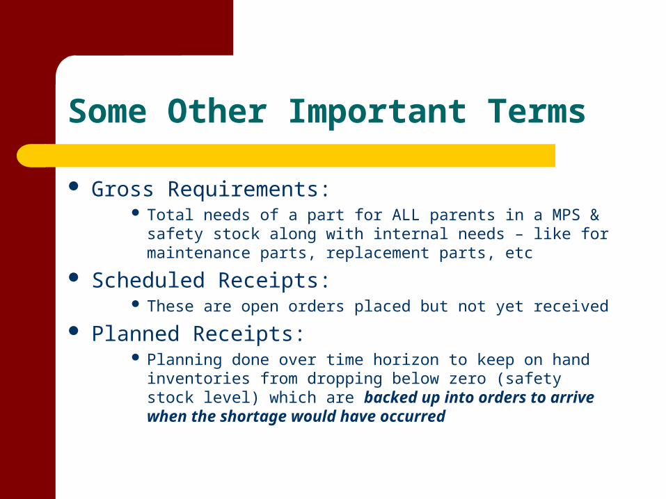
Some Other Important Terms

Gross Requirements: Total needs of a part for ALL parents in a MPS & safety stock

along with internal needs – like for maintenance parts, replacement parts, etc

Scheduled Receipts: These are open orders placed but not yet received

Planned Receipts: Planning done over time horizon to keep on hand inventories

from dropping below zero (safety stock level) which are backed up into orders to arrive when the shortage would have occurred

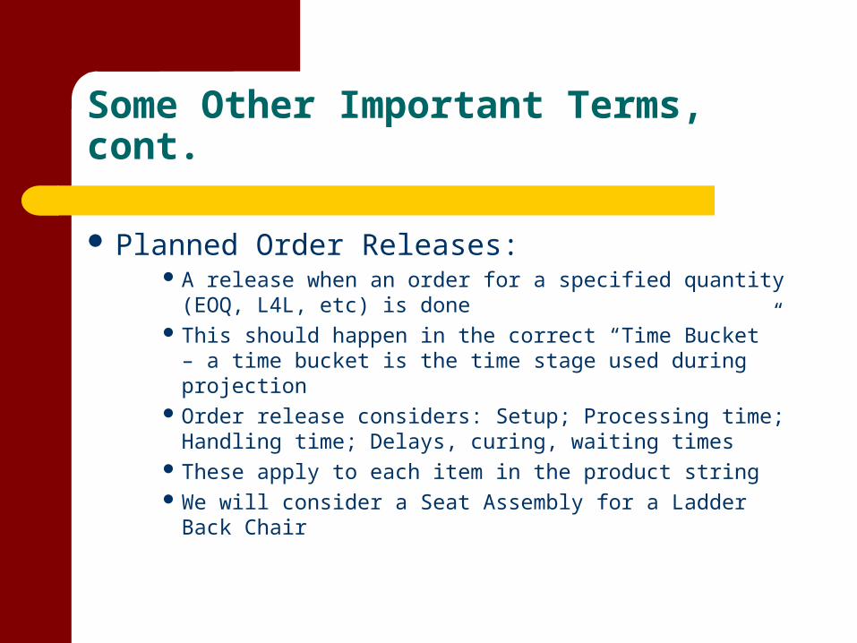
Some Other Important Terms, cont.

Planned Order Releases: A release when an order for a specified quantity (EOQ,

L4L, etc) is done This should happen in the correct “Time Bucket” – a

time bucket is the time stage used during projection Order release considers: Setup; Processing time;

Handling time; Delays, curing, waiting times These apply to each item in the product string We will consider a Seat Assembly for a Ladder Back

Chair

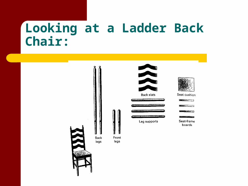
Looking at a Ladder Back Chair:

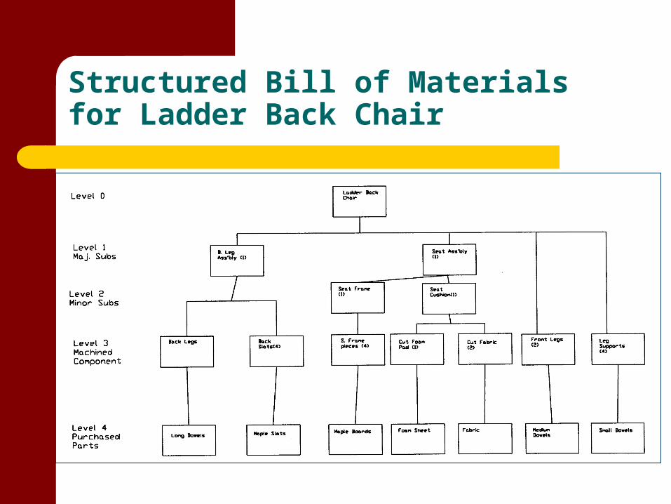
Structured Bill of Materials for Ladder Back Chair

Focusing on the Seat Assembly

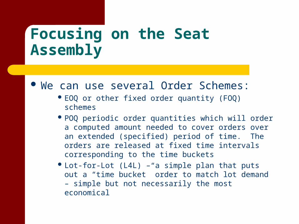
We can use several Order Schemes: EOQ or other fixed order quantity (FOQ) schemes POQ periodic order quantities which will order a

computed amount needed to cover orders over an extended (specified) period of time. The orders are released at fixed time intervals corresponding to the time buckets

Lot-for-Lot (L4L) – a simple plan that puts out a “time bucket” order to match lot demand – simple but not necessarily the most economical

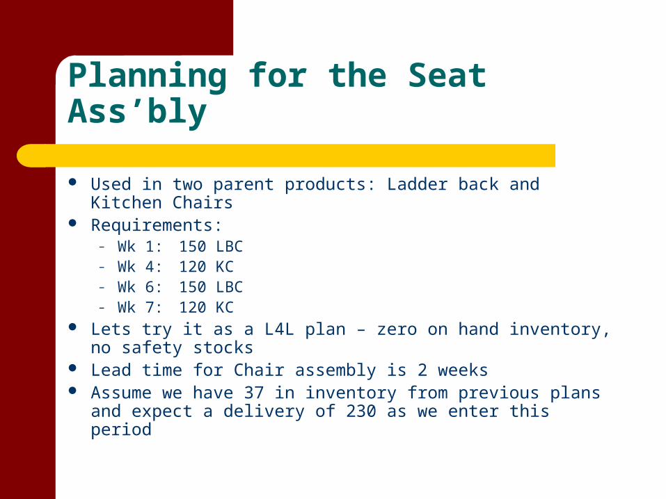
Planning for the Seat Ass’bly

Used in two parent products: Ladder back and Kitchen Chairs Requirements:

– Wk 1: 150 LBC– Wk 4: 120 KC– Wk 6: 150 LBC– Wk 7: 120 KC

Lets try it as a L4L plan – zero on hand inventory, no safety stocks

Lead time for Chair assembly is 2 weeks Assume we have 37 in inventory from previous plans and

expect a delivery of 230 as we enter this period

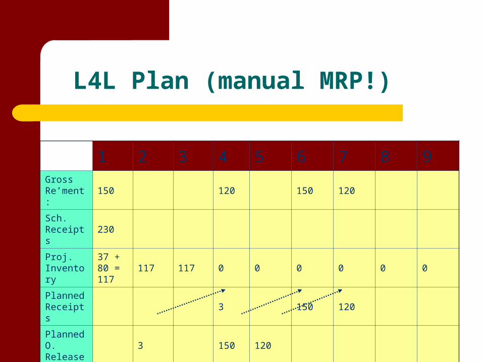
L4L Plan (manual MRP!)

1 2 3 4 5 6 7 8 9Gross Re’ment:

150 120 150 120

Sch. Receipts

230

Proj. Inventory

37 + 80 = 117

117 117 0 0 0 0 0 0

Planned Receipts

3 150 120

Planned O. Release

3 150 120

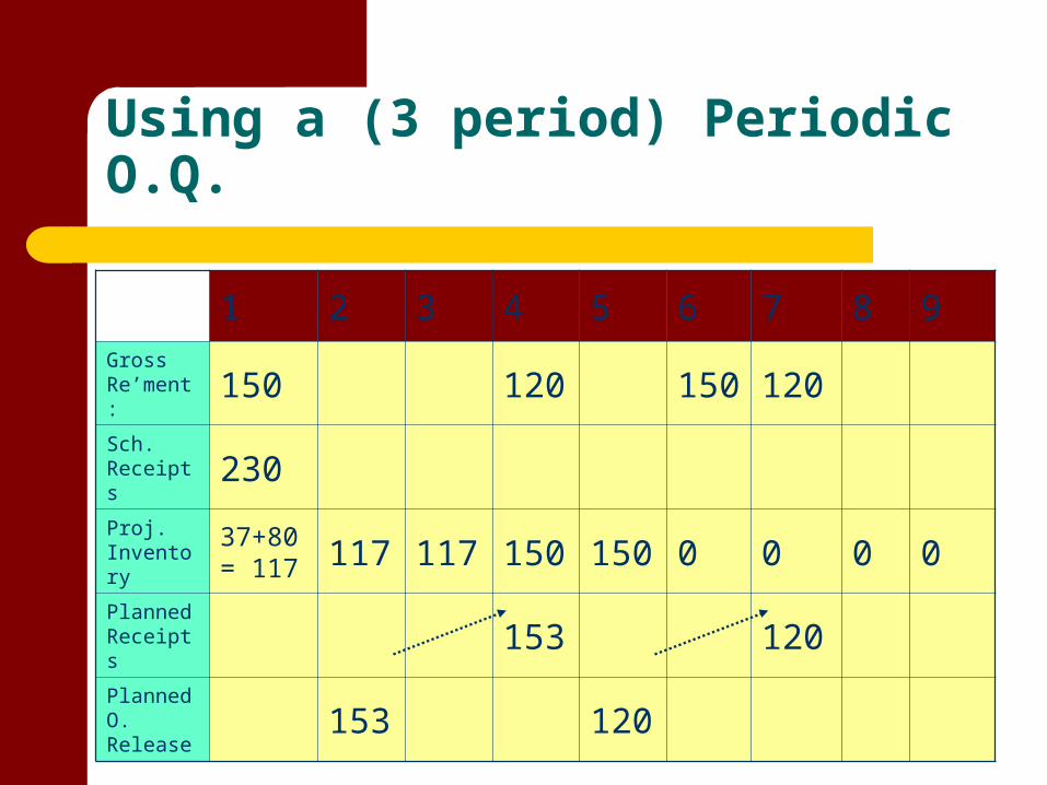
Using a (3 period) Periodic O.Q.

1 2 3 4 5 6 7 8 9

Gross Re’ment: 150 120 150 120

Sch. Receipts 230

Proj. Inventory

37+80 = 117 117 117 150 150 0 0 0 0

Planned Receipts 153 120Planned O. Release

153 120

Focusing on the “Periods”

Period 1 (1-2-3): needs are 150 Receipts/onhands are 230 + 37 Xs is 117 which enters inventory

Period 2 (4-5-6): needs are (120 + 150) = 270 units Less onhand (117) means we need 153 units for period

to arrive at start of period Release order in period two to arrive by period 4 – start

of second period

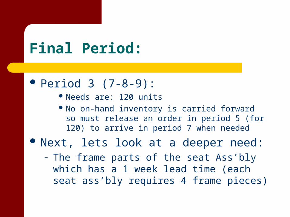
Final Period:

Period 3 (7-8-9): Needs are: 120 units No on-hand inventory is carried forward so must release

an order in period 5 (for 120) to arrive in period 7 when needed

Next, lets look at a deeper need:– The frame parts of the seat Ass’bly which has a 1

week lead time (each seat ass’bly requires 4 frame pieces)

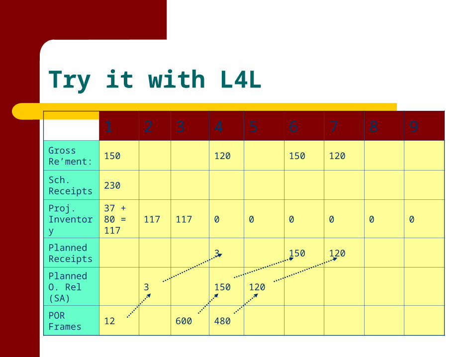
Try it with L4L

1 2 3 4 5 6 7 8 9Gross Re’ment:

150 120 150 120

Sch. Receipts

230

Proj. Inventory

37 + 80 = 117

117 117 0 0 0 0 0 0

Planned Receipts

3 150 120

Planned O. Rel (SA)

3 150 120

POR Frames

12 600 480

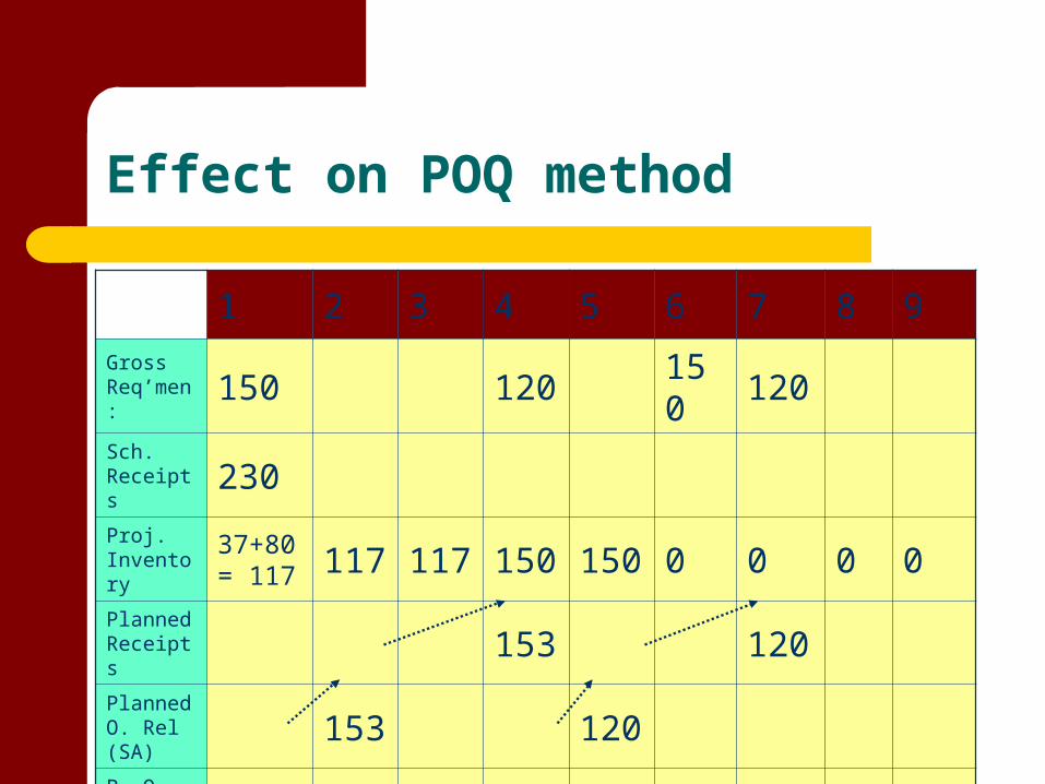
Effect on POQ method

1 2 3 4 5 6 7 8 9

Gross Req’men: 150 120 150 120

Sch. Receipts 230

Proj. Inventory

37+80 = 117 117 117 150 150 0 0 0 0

Planned Receipts 153 120Planned O. Rel (SA)

153 120

P. O. R. frames 612 480

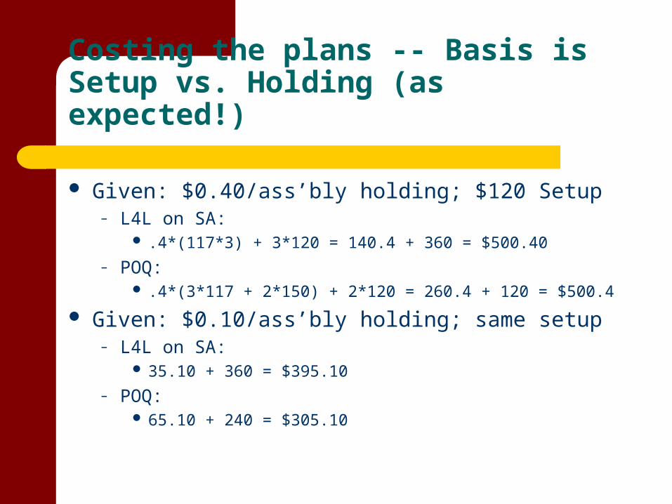
Costing the plans -- Basis is Setup vs. Holding (as expected!)

Given: $0.40/ass’bly holding; $120 Setup– L4L on SA:

.4*(117*3) + 3*120 = 140.4 + 360 = $500.40

– POQ: .4*(3*117 + 2*150) + 2*120 = 260.4 + 120 = $500.4

Given: $0.10/ass’bly holding; same setup– L4L on SA:

35.10 + 360 = $395.10

– POQ: 65.10 + 240 = $305.10

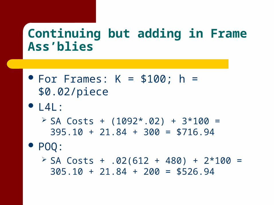
Continuing but adding in Frame Ass’blies

For Frames: K = $100; h = $0.02/piece L4L:

SA Costs + (1092*.02) + 3*100 = 395.10 + 21.84 + 300 = $716.94

POQ: SA Costs + .02(612 + 480) + 2*100 = 305.10 +

21.84 + 200 = $526.94

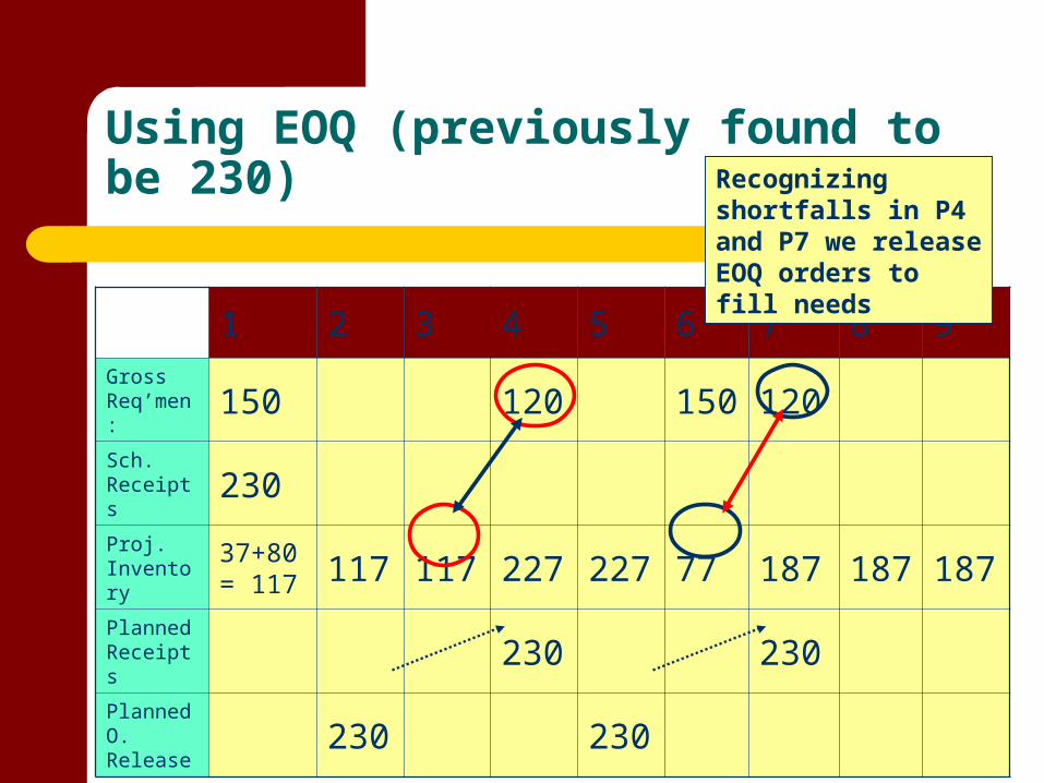
Using EOQ (previously found to be 230)

1 2 3 4 5 6 7 8 9

Gross Req’men: 150 120 150 120

Sch. Receipts 230

Proj. Inventory

37+80 = 117 117 117 227 227 77 187 187 187

Planned Receipts 230 230Planned O. Release

230 230

Recognizing shortfalls in P4 and P7 we release EOQ orders to fill needs

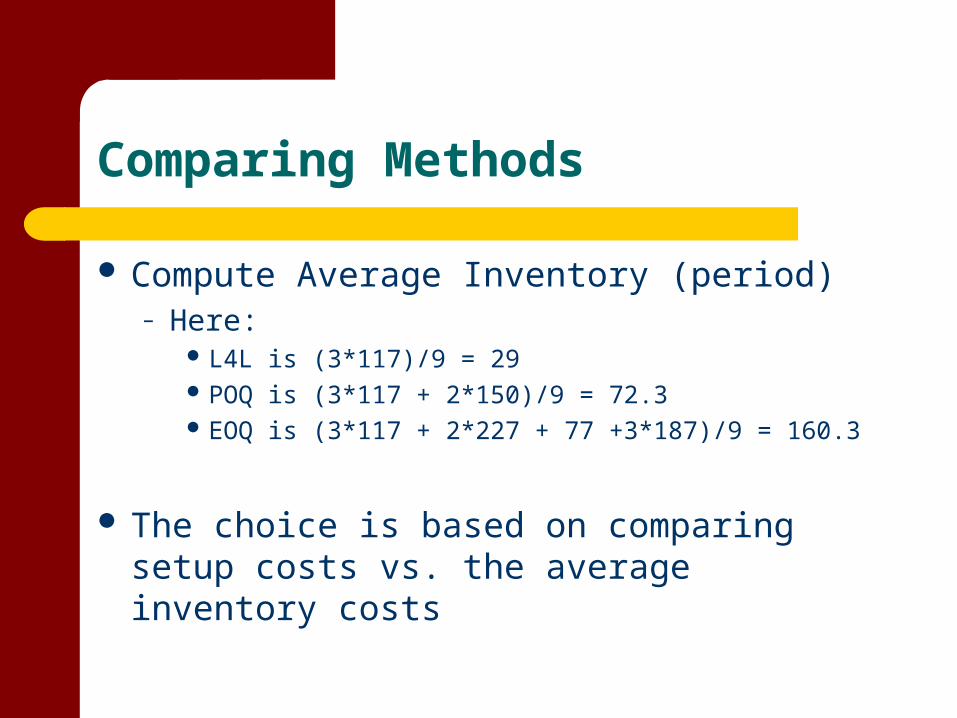
Comparing Methods

Compute Average Inventory (period)– Here:

L4L is (3*117)/9 = 29 POQ is (3*117 + 2*150)/9 = 72.3 EOQ is (3*117 + 2*227 + 77 +3*187)/9 = 160.3

The choice is based on comparing setup costs vs. the average inventory costs

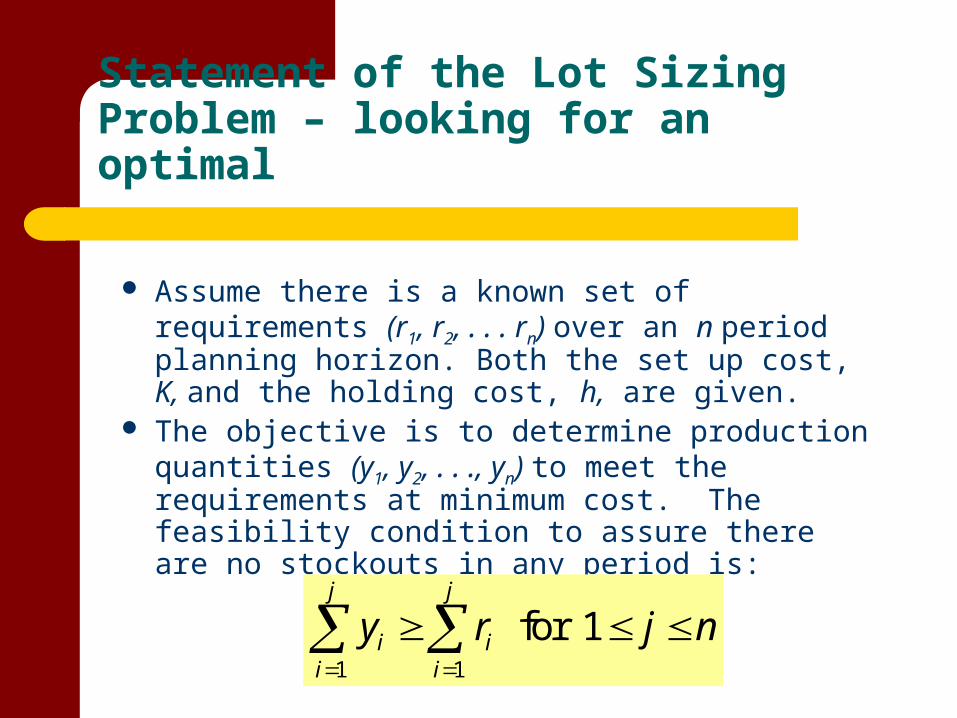
Statement of the Lot Sizing Problem – looking for an optimal

Assume there is a known set of requirements (r1, r2, . . . rn) over an n period planning horizon. Both the set up cost, K, and the holding cost, h, are given.

The objective is to determine production quantities (y1, y2, . . ., yn) to meet the requirements at minimum cost. The feasibility condition to assure there are no stockouts in any period is:

1 1

for 1j j

i ii i

y r j n

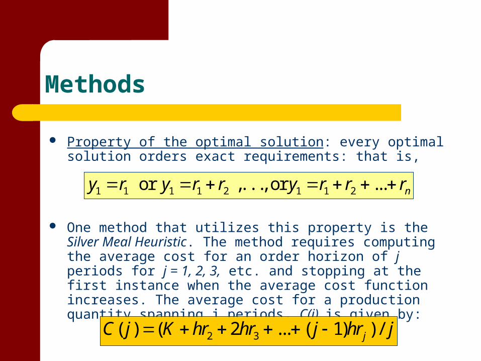
Methods

Property of the optimal solution: every optimal solution orders exact requirements: that is,

One method that utilizes this property is the Silver Meal Heuristic. The method requires computing the average cost for an order horizon of j periods for j = 1, 2, 3, etc. and stopping at the first instance when the average cost function increases. The average cost for a production quantity spanning j periods, C(j), is given by:

1 1 1 1 2 1 1 2 or ,. . ., or ... ny r y r r y r r r

2 3( ) ( 2 ... ( 1) ) /jC j K hr hr j hr j

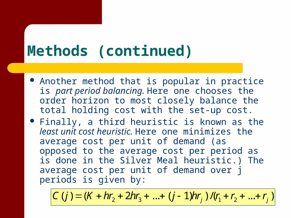
Methods (continued)

Another method that is popular in practice is part period balancing. Here one chooses the order horizon to most closely balance the total holding cost with the set-up cost.

Finally, a third heuristic is known as the least unit cost heuristic. Here one minimizes the average cost per unit of demand (as opposed to the average cost per period as is done in the Silver Meal heuristic.) The average cost per unit of demand over j periods is given by:

2 3 1 2( ) ( 2 ... ( 1) ) /( ... )j jC j K hr hr j hr r r r

Methods (concluded)

Experimental evidence seems to favor the Silver Meal Heuristic as the most cost efficient among the four discussed in the text.

Optimal lot sizes can be found by using backwards dynamic programming.

The (best?) heuristic method for lot sizing subject to capacity constraints is shown next

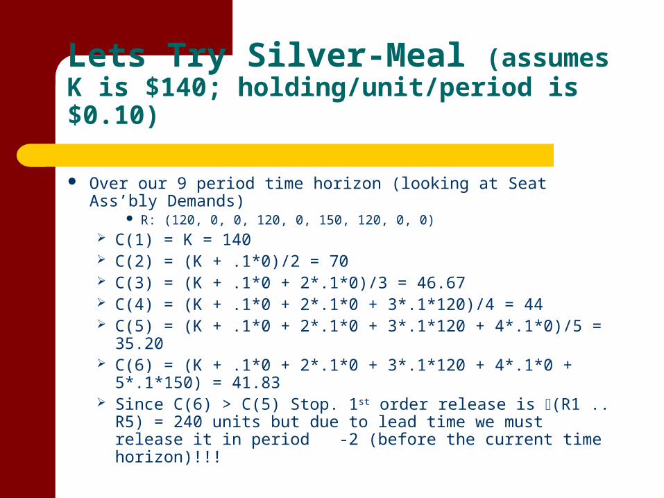
Lets Try Silver-Meal (assumes K is $140; holding/unit/period is $0.10)

Over our 9 period time horizon (looking at Seat Ass’bly Demands)

R: (120, 0, 0, 120, 0, 150, 120, 0, 0) C(1) = K = 140 C(2) = (K + .1*0)/2 = 70 C(3) = (K + .1*0 + 2*.1*0)/3 = 46.67 C(4) = (K + .1*0 + 2*.1*0 + 3*.1*120)/4 = 44 C(5) = (K + .1*0 + 2*.1*0 + 3*.1*120 + 4*.1*0)/5 = 35.20 C(6) = (K + .1*0 + 2*.1*0 + 3*.1*120 + 4*.1*0 + 5*.1*150) =

41.83 Since C(6) > C(5) Stop. 1st order release is (R1 .. R5) =

240 units but due to lead time we must release it in period -2 (before the current time horizon)!!!

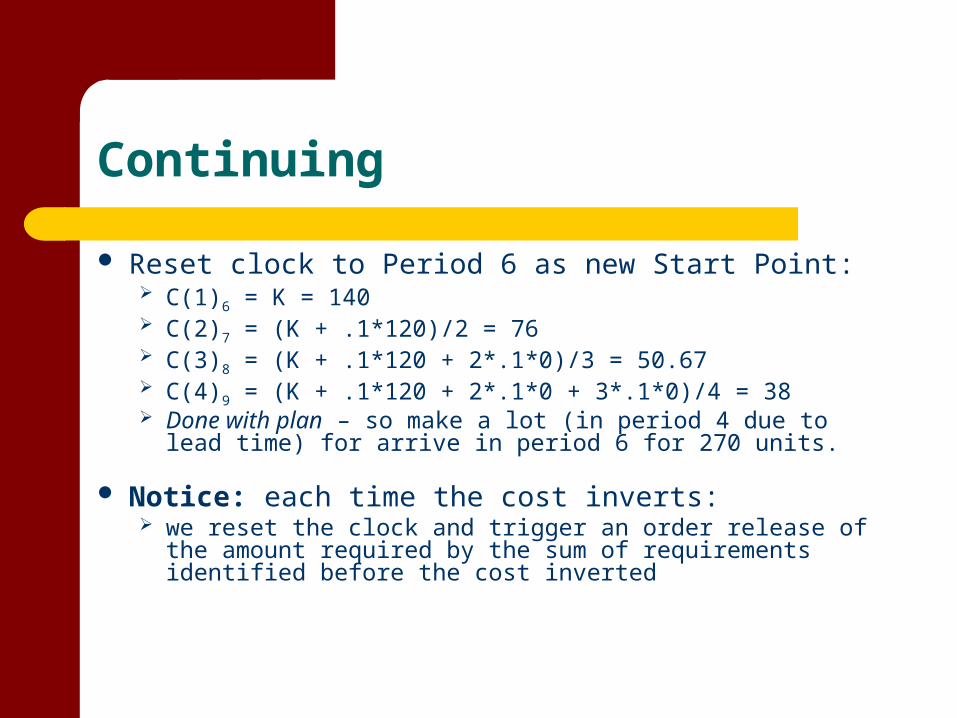
Continuing

Reset clock to Period 6 as new Start Point: C(1)6 = K = 140 C(2)7 = (K + .1*120)/2 = 76 C(3)8 = (K + .1*120 + 2*.1*0)/3 = 50.67 C(4)9 = (K + .1*120 + 2*.1*0 + 3*.1*0)/4 = 38 Done with plan – so make a lot (in period 4 due to lead

time) for arrive in period 6 for 270 units.

Notice: each time the cost inverts: we reset the clock and trigger an order release of the

amount required by the sum of requirements identified before the cost inverted

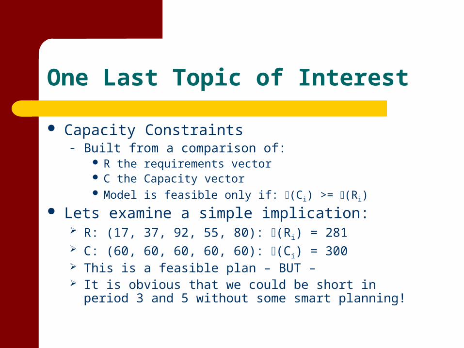
One Last Topic of Interest

Capacity Constraints– Built from a comparison of:

R the requirements vector C the Capacity vector Model is feasible only if: (Ci) >= (Ri)

Lets examine a simple implication: R: (17, 37, 92, 55, 80): (Ri) = 281 C: (60, 60, 60, 60, 60): (Ci) = 300 This is a feasible plan – BUT – It is obvious that we could be short in period 3 and 5 without

some smart planning!

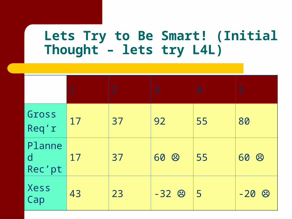
Lets Try to Be Smart! (Initial Thought – lets try L4L)

1 2 3 4 5

Gross

Req’r17 37 92 55 80

Planned Rec’pt

17 37 60 55 60

Xess Cap

43 23 -32 5 -20

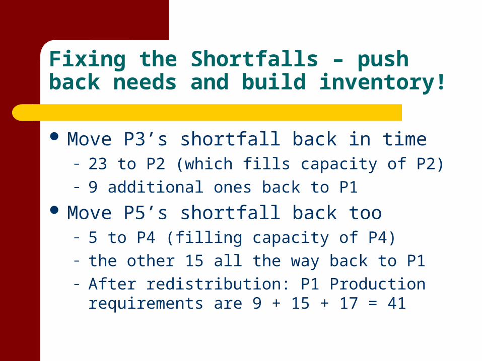
Fixing the Shortfalls – push back needs and build inventory!

Move P3’s shortfall back in time – 23 to P2 (which fills capacity of P2)– 9 additional ones back to P1

Move P5’s shortfall back too– 5 to P4 (filling capacity of P4) – the other 15 all the way back to P1 – After redistribution: P1 Production requirements are

9 + 15 + 17 = 41

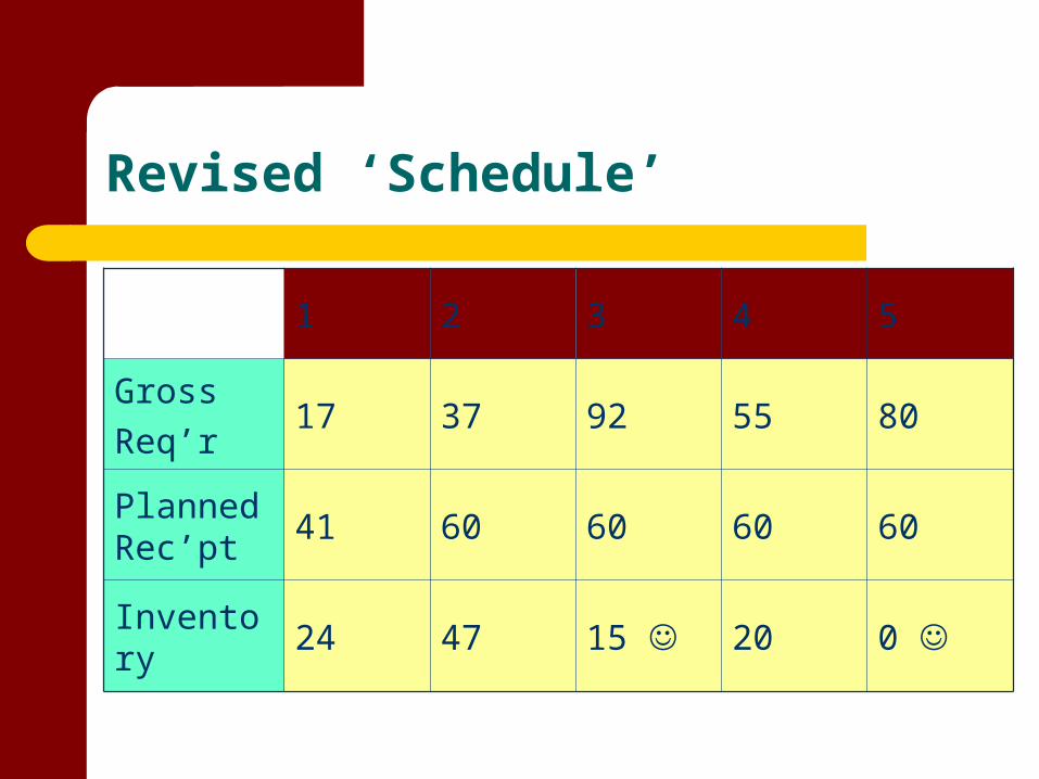
Revised ‘Schedule’

1 2 3 4 5

Gross

Req’r17 37 92 55 80

Planned Rec’pt

41 60 60 60 60

Inventory 24 47 15 20 0

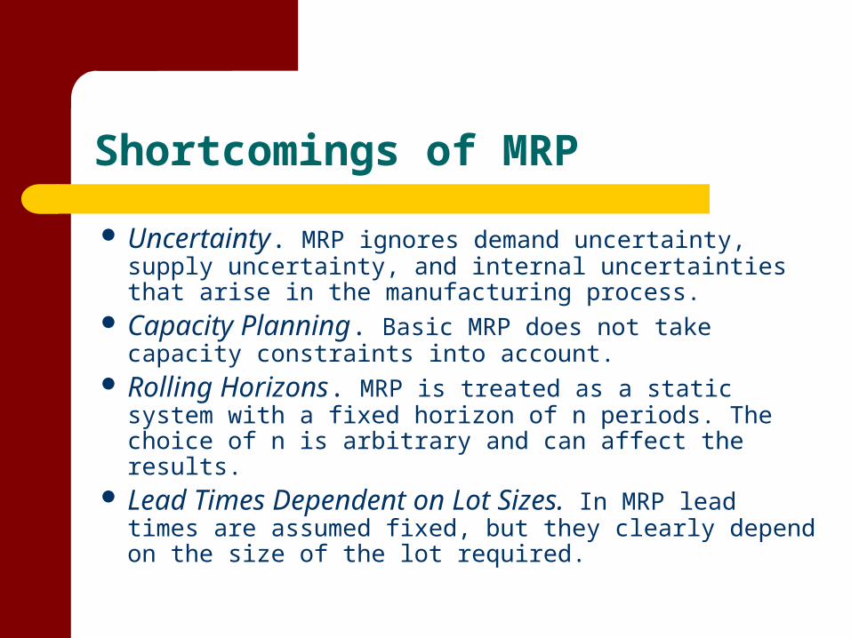
Shortcomings of MRP

Uncertainty. MRP ignores demand uncertainty, supply uncertainty, and internal uncertainties that arise in the manufacturing process.

Capacity Planning. Basic MRP does not take capacity constraints into account.

Rolling Horizons. MRP is treated as a static system with a fixed horizon of n periods. The choice of n is arbitrary and can affect the results.

Lead Times Dependent on Lot Sizes. In MRP lead times are assumed fixed, but they clearly depend on the size of the lot required.

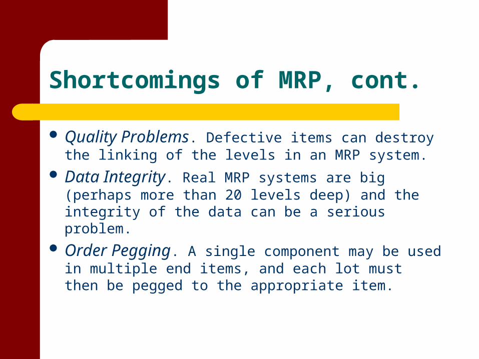
Shortcomings of MRP, cont.

Quality Problems. Defective items can destroy the linking of the levels in an MRP system.

Data Integrity. Real MRP systems are big (perhaps more than 20 levels deep) and the integrity of the data can be a serious problem.

Order Pegging. A single component may be used in multiple end items, and each lot must then be pegged to the appropriate item.