Roadmap Based Pursuit-Evasion and CollisionAvoidance

Volkan Isler, Dengfeng Sun and Shankar SastryCITRIS

University of California Berkeley, CA, 94720Email: {isler,sundf,sastry}@eecs.berkeley.edu

Abstract— We study pursuit-evasion games for mobile robotsand their applications to collision avoidance. In the first partof the paper, under the assumption that the pursuer and theevader (possibly subject to physical constraints) share the sameroadmap to plan their strategies, we present sound and completestrategies for three different games. In the second part, we utilizethe pursuit-evasion results to post-process the workspace and/orconfiguration space and obtain a collision probability map ofthe environment. Next, we present a probabilistic method toutilize this map and plan trajectories which minimize the collisionprobability for independent robots.

I. I NTRODUCTION

Motion planning is one of the fundamental problems inrobotics. Broadly speaking, it is the problem of selecting aset of actions or controls which, upon execution, would takethe robot from a given initial state to a given final state.

Motion planning is a challenging problem whose complex-ity stems primarily from two sources: environment complexityand system complexity. The former refers to the complexityof planning trajectories for perhaps simple robots but incomplex environments. For example, finding shortest pathsin 3D is an NP-hard problem [1]. By system complexity,we refer to the complexity of planning trajectories for com-plex, high degree-of-freedom systems even in the absence ofobstacles. Traditionally, the former complexity is addressedby algorithmic/combinatorial techniques and data structures(e.g. Dijkstra’s algorithm on visibility graphs) whereas thelatter type of complexity is addressed using control-theoretictechniques.

Developing techniques that address both types of complex-ity has been the focus of significant recent research (see [2],[3] for an overview). Notable success has been achieved bysampling-based roadmap methods [4], [5] which we review inSection II.

In this paper, we present algorithms which solve two dy-namic motion planning problems that take place on roadmaps:pursuit-evasion and collision avoidance.

In the first part of the paper, we study pursuit-evasion gamesthat take place on roadmaps. In a pursuit-evasion game, apursuer tries to capture an evader while the evader is tryingtoavoid capture. In robotics, solutions to pursuit-evasion gamesare used to obtain worst-case guarantees to collision-avoidanceproblems and, in general, to motion planning in dynamic envi-ronments. For example, suppose two robots are independentlyoperating in the same workspace. When there is a danger of

collision, each robot can execute an evasion strategy obtainedas the solution of a pursuit-evasion game where the other robotacts as a pursuer trying to collide. Such a solution wouldguarantee that each robot will avoid collision regardless of theactions of the other robot. In Section III, we present solutionsto pursuit-evasion games on roadmaps. Our model studiesinteractions between a pursuer and an evader who use thesame roadmap to plan their trajectories. Under this assumption,we present algorithms based on the dynamic programmingprinciple to generatesound and completestrategies for bothplayers.

The pursuit-evasion models we study in the first part assumethat the players haveglobally conflicting objectives. In thismodel, the pursuer is truly adversarial and its objective istocollide with the evader. In most motion-planning settings,sucha model can be too strict for modeling collision-avoidance.Typically, robots plan their trajectories independently.How-ever, when they get close to each other, they may switch to areactive collision-avoidance mode and become unpredictable.At this point, it is desirable to have the worst-case guaranteesgiven by the game theoretic formulation. In the second part ofthe paper (Section IV) we propose a model for such scenarios.In this formulation, independent (neither collaborating norconflicting) agents operate in the workspace while avoidingcollisions locally. We utilize the results of the first part todefinelocal pursuit-evasion gameswhere the players react toeach other only when they are within a given interaction zone.Under this model we show how• the workspace and/or configuration space can be post-

processed to obtain a collision probability map of theenvironment,

• the players can compute worst-case collision avoidancestrategies after they are enter the interaction zone, and

• compute optimal trajectories that minimize the expectedprobability of a collision.

We start with an overview of related literature.

A. Related work

Due to their many applications, literature on pursuit-evasiongames is vast. To model the adversarial nature of the game,pursuit-evasion games are usually studied in a game theoreticframework [6], [7]. The conditions under which the pursuercan capture the evader are obtained by studying a Hamilton-Jacobi-Isaacs equation which brings together the system equa-

tions of the pursuer and the evader. This approach has theadvantage of yielding a closed-form solution of the game.Unfortunately, as the environments get complicated, solvingHamilton-Jacobi-Isaacs equations become intractable.

Recently, there has been increasing interest in developingpursuit strategies (which incorporate sensing limitations) tocapture intelligent evaders contaminating a complex environ-ment [8], [9], [10].

In robotics, complex environments are modeled eithertopologically (usually with a graph-based representation)or geometrically (usually a polygonal/polyhedral representa-tion). Classical work on pursuit-evasion games on graphsincludes [11], [12], [13], [14]. See [15], [16] for recent results.Pursuit-evasion games in polygonal environments are also wellstudied. See [17], [18], [19] and recently [20], [21], [22].

As mentioned earlier, solving pursuit-evasion games be-tween robots subject to physical constraints (such as turningradius) which takes place in a complex environment is verychallenging. Note that such problems inherit all difficulties oftraditional motion-planning. To tackle these two difficulties,our approach in this paper is to reduce a game between tworobots subject to physical constraints to a pursuit-evasion gamethat takes place on a graph, a.k.a. the roadmap. We defer thedetails to Section II.

Our work is also directly related to the work in multi-robotplanning and collision avoidance. For basic results in multiplerobot planning see [23]. For recent work in collision avoidanceand multi-robot planning see [24], [25], [26], [27]. Recentresearch on extending the probabilistic roadmap frameworktomulti-robot and dynamically changing environments can befound in [28], [29], [30], [31].

II. N OTATION AND PRELIMINARIES

In this section, we present the main concepts and thenotation used throughout the paper. LetC be the configurationspace of a robot. We assume that we are given a discreteset of pointsC that represent the configuration space. Such aset can be obtained, for example, by randomly sampling theconfiguration space as in the case of probabilistic roadmapsorby putting a grid on the configuration space which is practicalfor low dimensional configuration spaces. When the robot isin a configurationc∈C, we use the notationW(c) to denotethe subset of the workspace occupied by the robot.

We are also givenU = {u1, . . . ,uK}, a set of deterministic,‘simple’ controllers for the robot. Given two arbitrary configu-rationsci ,c j ∈ C , the notationci→u c j is interpreted as:whenin configuration ci , if the robot executes controller u∈U, itreaches configuration cj in a single time unit.The significanceof the simplicity of the controllers inU lies in easy verificationof ci →u c j for arbitrary configurations.

The main data structure that will be utilized throughout thepaper is the notion of atimed roadmap. A timed roadmap isa graphG = (V,E). The vertex setV is given by the discretesampling of the configuration space,V = C . Let c : V→ C bea bijection such thatc(v) returns the configuration associatedwith the vertexv. The edge setE is obtained as follows:

For any vi ,v j ∈ V, the edge(vi ,v j) ∈ E if and only if thereexists a simple controlleru∈U such thatc(vi)→u c(v j). Thefunction u : E→U returns the controller associated with anedge1. For a given vertexv, N(v) = {v′ : (v,v′) ∈ E} denotesthe neighborhood ofv.

For we are interested in pairwise interactions between therobots, we define thestatic interaction spaceIs = {(vi ,v j) :vi ,v j ∈ V}. Similarly, the dynamic interaction spaceId ={(ei ,ej) : ei ,ej ∈E}. For pursuit-evasion games, we assume theavailability of a capture function,capture: Id→{true, f alse}which, given (ei ,ej) ∈ Id with ei = (vi ,v′i) and ej = (v j ,v′j),capture((ei ,ej)) returns true if and only if capture occurswhile the first robot is executingvi →u(ei) v′i and the secondrobot is executingv j →u(ej ) v′j . Again, the simplicity of thecontrollers become a crucial factor in computing the capturefunction. In addition, note that for simplicity of notationweassume that the robots use the same roadmap for planningtheir trajectories2.

We demonstrate these concepts with the well-known Dubinscar, which will be used as an ongoing example for the pursuit-evasion results.

A. Dubins Vehicle

We model each agent as a Dubins car by assuming that anagent moves at a constant forward speedus and its maximumsteering angle isφmax, which results in a minimum turningradius ρmin. As the agent travels, its movement is governedby the following dynamics:

x(t) = uscosθ(t)

y(t) = ussinθ(t)

θ(t) = u

(1)

where (x(t),y(t)) ∈ R2 is the position of the agent at time

t and θ(t) is the orientation;u is chosen from the intervalU = [− tanφmax, tanφmax].

Let us define three motion primitives such that in eachmotion primitive a constant steeringu is applied:

Symbol S L RSteeringu 0 −umax umax

S primitive means that an agent moves straight ahead, whileL and R primitives mean that an agent turns as sharply aspossible to the left and right, respectively. The primitiveCrefers to eitherL or R.

Dubins showed in [32] that given any two configurationsc1

and c2, the shortest path can be expressed as a combinationof no more than three of these motion primitives. Dubinsalso showed that only six “words” (combinations of the threemotion primitives) are possible:

{LRL,RLR,LSL,RSL,LSR,RSR}. (2)

1We assume that there is a unique controller associated with each edge andambiguities are resolved arbitrarily.

2If there are two different roadmaps, we simply define the interaction spaceas the product of these two graphs.

For the Dubin’s car, we start with a discretization ofthe configuration spaceW × SO(1) where W denotes theworkspace. We restrict ourselves to three types of basiccontrollers corresponding to each motion primitive: “turnleftα degrees for 1 time-unit”, “turn rightα degrees for 1 timeunit” and “move straight” for 1 time unit. We connect twoconfigurationsci ,c j if there c j is reachable fromci by theexecution of a simple controller.

Figure 1 shows a simple workspace and the shortest trajec-tory of an agent moving from configurationc1 = [2,2, π

2 ] toc2 = [14,8, π

2 ]. In this scenario, the orientation angles inC arecoarsely discretized byπ/2.

0 2 4 6 8 10 12 14 16

0

2

4

6

8

10

Fig. 1. An agent moves fromc1 to c2. Diamonds mark the intermediateconfigurations the agent passes inC . Obstacles exist in the areas markedblack.

Collision detection:We define asafety distance rs such thatwhenever the distance between agentss1 and s2 is less thanrs, collision occurs. Notice that in practicers is time varyingdepending on both positions and orientations of the agents.In this paper we assume that the agents are in the form ofdiscs and assume that the radius of an agent isr. In this case,rs = 2r.

Since every trajectory of an agent is a combination of themotion primitives, for collision detection between agents, itis enough to check whether there is collision between anyC−C, C−S andS−S primitives along the two trajectories ofthe agents.

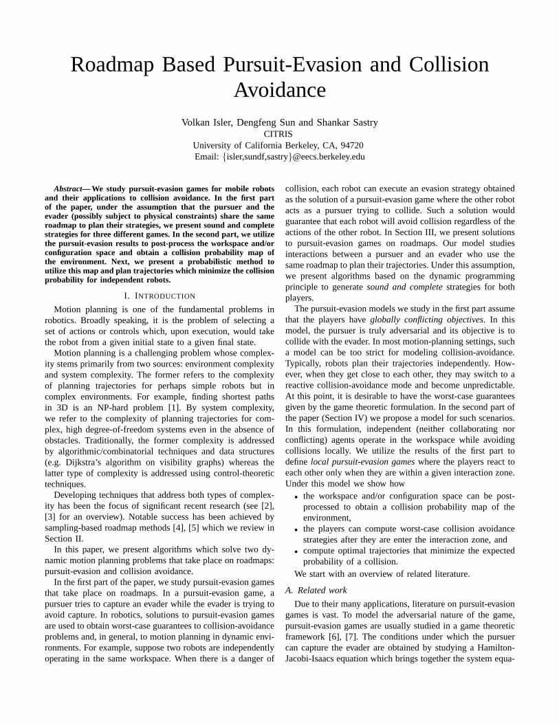
θ0

α

(xc,yc)

c0, t0

Lα

ρ

c1, t1

Fig. 2. L primitive

Consider the curve of anL primitive centered at(xc,yc)in Figure 2. The curveLα starts from configurationc0 =(x0,y0,

π2 + θ0) at time t0 and ends at configurationc1 =

(x1,y1,π2 + θ0 + α) at time t1. Without loss of generality,

assumet0 = 0, t1 = Ts. The coordinates(x(t),y(t)) at timet ∈ [0,Ts] can be derived as:

x(t) = xc +ρcos(umaxt +θ0)

y(t) = yc +ρsin(umaxt +θ0)(3)

Similarly for anR primitive, we have

x(t) = xc +ρcos(−umaxt +θ0)

y(t) = yc +ρsin(−umaxt +θ0)(4)

In the following, we useL primitive as a representative forC type primitives. A similar result can be derived forRprimitives.

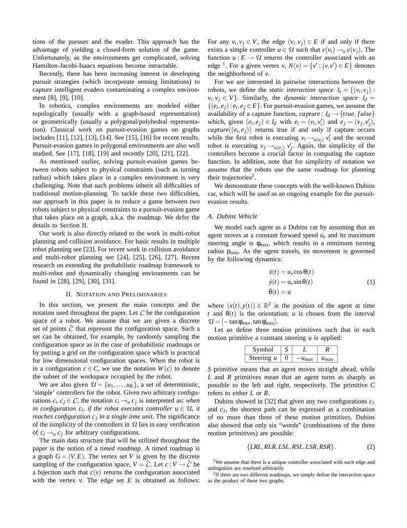
c0, t0

c1, t1

θ0

Fig. 3. S primitive

An S primitive is shown in Figure 3, which starts atc0 =(x0,y0,θ0) and ends atc1 = (x1,y1,θ0). The coordinates attare (again, we assumet0 = 0, t1 = Ts)

x(t) = x0 +ust cosθ0

y(t) = y0 +ust sinθ0(5)

Suppose the positions ofs1 and s2 are (x1(t),y1(t)) and(x2(t),y2(t)) at time t. The distance betweens1 ands2 is

d(t) =√

[x1(t)−x2(t)]2 +[y1(t)−y2(t)]2. (6)

wherexi(t),yi(t), i = 1,2, are defined in Equations (3, 4, 5).Clearly d(t) is a continuous function on[0,Ts]. To detect ifcollision exists, it is enough to check if

mint∈[0,Ts]

d(t) < rs. (7)

III. SOLUTIONS TO TYPICAL PURSUIT-EVASION PROBLEMS

USING THE TIMED-ROADMAP

In this section, we show how typical pursuit-evasion prob-lems can be solved when the motion-plans of the players arerestricted to the timed-roadmap.

We use the following formulation for all the games weconsider. The games take place between a pursuerP andevaderE . We assume that the players are identical and theyplan their trajectories using the same timed-roadmap (Hence,they use the same controller setU). In this section, weconsider games with full state information where the playerscan observe each other’s configuration throughout the game.We begin with the following basic version:

GAME 1: Given initial configurationsp0 and e0, can P

eventually collide withE?The algorithm in Table I allows us to preprocess the

static interaction space and answer this query for all initialconditions.

After the execution of the algorithm, the variable(p,e).timestampis set to the number of time-steps to a colli-sion after the pursuer and the evader reach the configurationsp and e respectively. The following two lemmas show thatAlgorithm Collision-Detection can used to solve GAME 1in a sound and complete fashion. We assume, without lossof generality, that the evader wants to maximize the time tocollision and the pursuer wants to minimize it.

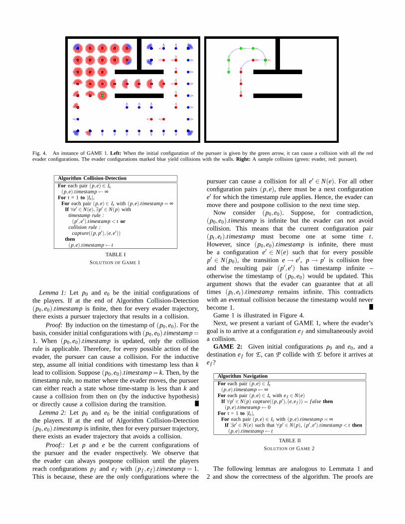
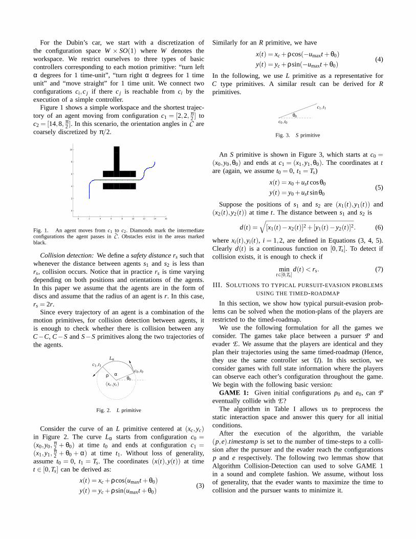
Fig. 4. An instance of GAME 1.Left: When the initial configuration of the pursuer is given by the green arrow, it can cause a collision with all the redevader configurations. The evader configurations marked blueyield collisions with the walls.Right: A sample collision (green: evader, red: pursuer).

Algorithm Collision-DetectionFor each pair(p,e) ∈ Is

(p,e).timestamp← ∞For t = 1 to |Is|,

For each pair(p,e) ∈ Is with (p,e).timestamp= ∞If ∀e′ ∈ N(e),∃p′ ∈ N(p) with

timestamp rule :(p′,e′).timestamp< t or

collision rule :capture((p, p′),(e,e′))

then(p,e).timestamp← t

TABLE I

SOLUTION OF GAME 1

Lemma 1:Let p0 and e0 be the initial configurations ofthe players. If at the end of Algorithm Collision-Detection(p0,e0).timestampis finite, then for every evader trajectory,there exists a pursuer trajectory that results in a collision.

Proof: By induction on the timestamp of(p0,e0). For thebasis, consider initial configurations with(p0,e0).timestamp=1. When (p0,e0).timestampis updated, only the collisionrule is applicable. Therefore, for every possible action oftheevader, the pursuer can cause a collision. For the inductivestep, assume all initial conditions with timestamp less than klead to collision. Suppose(p0,e0).timestamp= k. Then, by thetimestamp rule, no matter where the evader moves, the pursuercan either reach a state whose time-stamp is less thank andcause a collision from then on (by the inductive hypothesis)or directly cause a collision during the transition.

Lemma 2:Let p0 and e0 be the initial configurations ofthe players. If at the end of Algorithm Collision-Detection(p0,e0).timestampis infinite, then for every pursuer trajectory,there exists an evader trajectory that avoids a collision.

Proof:: Let p and e be the current configurations ofthe pursuer and the evader respectively. We observe thatthe evader can always postpone collision until the playersreach configurationspf and ef with (pf ,ef ).timestamp= 1.This is because, these are the only configurations where the

pursuer can cause a collision for alle′ ∈ N(e). For all otherconfiguration pairs(p,e), there must be a next configuratione′ for which the timestamp rule applies. Hence, the evader canmove there and postpone collision to the next time step.

Now consider (p0,e0). Suppose, for contradiction,(p0,e0).timestampis infinite but the evader can not avoidcollision. This means that the current configuration pair(pt ,et).timestamp must become one at some timet.However, since(p0,e0).timestamp is infinite, there mustbe a configuratione′ ∈ N(e) such that for every possiblep′ ∈ N(p0), the transitione→ e′, p→ p′ is collision freeand the resulting pair(p′,e′) has timestamp infinite –otherwise the timestamp of(p0,e0) would be updated. Thisargument shows that the evader can guarantee that at alltimes (pt ,et).timestamp remains infinite. This contradictswith an eventual collision because the timestamp would neverbecome 1.

Game 1 is illustrated in Figure 4.Next, we present a variant of GAME 1, where the evader’s

goal is to arrive at a configurationef and simultaneously avoida collision.

GAME 2: Given initial configurationsp0 and e0, and adestinationef for E , canP collide with E before it arrives atef ?

Algorithm NavigationFor each pair(p,e) ∈ Is

(p,e).timestamp← ∞For each pair(p,e) ∈ Is with ef ∈ N(e)

If ∀p′ ∈ N(p) capture((p, p′),(e,ef )) = f alse then(p,e).timestamp← 0

For t = 1 to |Is|,For each pair(p,e) ∈ Is with (p,e).timestamp= ∞

If ∃e′ ∈ N(e) such that∀p′ ∈ N(p), (p′,e′).timestamp< t then(p,e).timestamp← t

TABLE II

SOLUTION OF GAME 2

The following lemmas are analogous to Lemmata 1 and2 and show the correctness of the algorithm. The proofs are

similar and hence omitted.Lemma 3:Let p0 and e0 be the initial configurations

of the players. If at the end of Algorithm Navigation,(p0,e0).timestamp= k < ∞, then the evader can reachef in ksteps while avoiding a collision.

Lemma 4:Let p0 and e0 be the initial configurationsof the players. If at the end of Algorithm Navigation(p0,e0).timestampis infinite, then the pursuer can collide withthe evader before it reachesef .

Finally, we present the solution of a dog-fight game. Firstwe define the capture condition.capture((p, p′),(e,e′)) is trueif and only if:

(i) during the transition fromp to p′, the angle between theheading of the pursuer and the ray from the pursuer to theevader becomes less than a threshold

(ii) the distance between the players is less than a threshold(iii) there are no obstacles between the playersWe are now ready to define the dog-fight game:GAME 3: Given initial configurationsp0 and e0, can E

captureP beforeP capturesE?Note that during a dog-fight, the roles of the pursuer and the

evader are not uniquely defined. The players must both avoida capture and capture simultaneously. However, AlgorithmCollision-Detection can be modified to solve GAME 3 asfollows. We run the algorithm with the modified capturefunction.

Algorithm DogFightFor each pair(p,e) ∈ Is

(p,e).timestamp← ∞For t = 1 to |Is|,

For each pair(p,e) ∈ Is with (p,e).timestamp= ∞If ∀e′ ∈ N(e),∃p′ ∈ N(p) with

timestamp rule :(p′,e′).timestamp< (e′, p′).timestampor

collision rule :capture((p, p′),(e,e′))

then(p,e).timestamp← t

TABLE III

SOLUTION OF GAME 3

Lemma 5:Let p0 ande0 be the initial configurations ofPandE respectively.

(i) If at the end of Algorithm Collision-Detection(p0,e0).timestamp≤ (e0, p0).timestamp, thenP wins the dog-fight game.

(ii) If, (p0,e0).timestamp≥ (e0, p0).timestamp, thenE winsthe dog-fight game.

The proof of Lemma 5 is similar to the proof of Lemma 1.Note that, it is possible to have(p0,e0).timestamp=

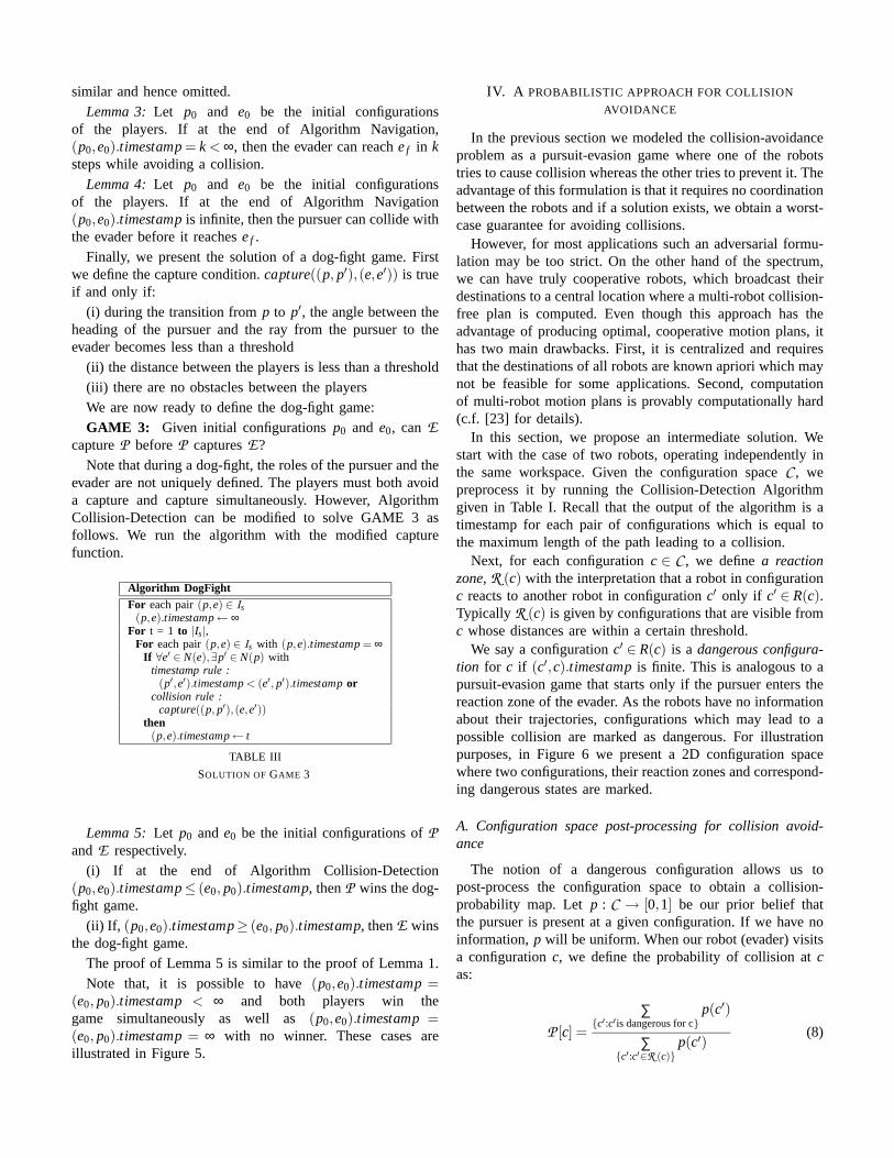
(e0, p0).timestamp < ∞ and both players win thegame simultaneously as well as(p0,e0).timestamp=(e0, p0).timestamp= ∞ with no winner. These cases areillustrated in Figure 5.

IV. A PROBABILISTIC APPROACH FOR COLLISION

AVOIDANCE

In the previous section we modeled the collision-avoidanceproblem as a pursuit-evasion game where one of the robotstries to cause collision whereas the other tries to prevent it. Theadvantage of this formulation is that it requires no coordinationbetween the robots and if a solution exists, we obtain a worst-case guarantee for avoiding collisions.

However, for most applications such an adversarial formu-lation may be too strict. On the other hand of the spectrum,we can have truly cooperative robots, which broadcast theirdestinations to a central location where a multi-robot collision-free plan is computed. Even though this approach has theadvantage of producing optimal, cooperative motion plans,ithas two main drawbacks. First, it is centralized and requiresthat the destinations of all robots are known apriori which maynot be feasible for some applications. Second, computationof multi-robot motion plans is provably computationally hard(c.f. [23] for details).

In this section, we propose an intermediate solution. Westart with the case of two robots, operating independently inthe same workspace. Given the configuration spaceC , wepreprocess it by running the Collision-Detection Algorithmgiven in Table I. Recall that the output of the algorithm is atimestamp for each pair of configurations which is equal tothe maximum length of the path leading to a collision.

Next, for each configurationc ∈ C , we definea reactionzone, R (c) with the interpretation that a robot in configurationc reacts to another robot in configurationc′ only if c′ ∈ R(c).Typically R (c) is given by configurations that are visible fromc whose distances are within a certain threshold.

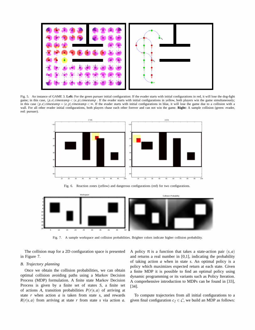
We say a configurationc′ ∈ R(c) is a dangerous configura-tion for c if (c′,c).timestampis finite. This is analogous to apursuit-evasion game that starts only if the pursuer entersthereaction zone of the evader. As the robots have no informationabout their trajectories, configurations which may lead to apossible collision are marked as dangerous. For illustrationpurposes, in Figure 6 we present a 2D configuration spacewhere two configurations, their reaction zones and correspond-ing dangerous states are marked.

A. Configuration space post-processing for collision avoid-ance

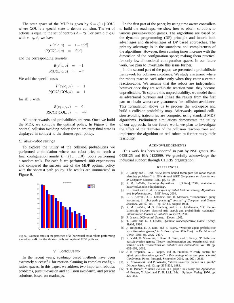
The notion of a dangerous configuration allows us topost-process the configuration space to obtain a collision-probability map. Letp : C → [0,1] be our prior belief thatthe pursuer is present at a given configuration. If we have noinformation,p will be uniform. When our robot (evader) visitsa configurationc, we define the probability of collision atcas:

P [c] =

∑{c′:c′is dangerous for c}

p(c′)

∑{c′:c′∈R (c)}

p(c′)(8)

p0

e0

Fig. 5. An instance of GAME 3.Left: For the green pursuer initial configuration: If the evader starts with initial configurations in red, it will lose the dog-fightgame; in this case,(p,e).timestamp< (e, p).timestamp. If the evader starts with initial configurations in yellow,both players win the game simultaneously;in this case(p,e).timestamp= (e, p).timestamp< ∞. If the evader starts with initial configurations in blue, itwill lose the game due to a collision with awall. For all other evader initial configurations, both players chase each other forever and can not win the game.Right: A sample collision (green: evader,red: pursuer).

(7,58)

10 20 30 40 50 60 70 80 90 100

−10

0

10

20

30

40

50

60

(10,8)

10 20 30 40 50 60 70 80 90 100

−10

0

10

20

30

40

50

60

Fig. 6. Reaction zones (yellow) and dangerous configurations (red) for two configurations.

Workspace

5 10 15 20 25 30 35 40 45 50

2

4

6

8

10

12

14

16

18

20

Collision Probability

Fig. 7. A sample workspace and collision probabilities. Brighter colors indicate higher collision probability.

The collision map for a 2D configuration space is presentedin Figure 7.

B. Trajectory planning

Once we obtain the collision probabilities, we can obtainoptimal collision avoiding paths using a Markov DecisionProcess (MDP) formulation. A finite state Markov DecisionProcess is given by a finite set of statesS, a finite setof actions A, transition probabilitiesP(r|s,a) of arriving atstate r when actiona is taken from states, and rewardsR(r|s,a) from arriving at stater from states via action a.

A policy π is a function that takes a state-action pair(s,a)and returns a real number in [0,1], indicating the probabilityof taking actiona when in states. An optimal policy is apolicy which maximizes expected return at each state. Givena finite MDP it is possible to find an optimal policy usingdynamic programming or its variants such as Policy Iteration.A comprehensive introduction to MDPs can be found in [33],[34].

To compute trajectories from all initial configurations to agiven final configurationcf ∈ C , we build an MDP as follows:

The state space of the MDP is given byS= C ∪{COL}whereCOL is a special state to denote collision. The set ofactions is equal to the set of controlsA= U. For eachc,c′ ∈Cwith c→u c′, we have

P(c′|c,u) = 1−P [c′]

P(COL|c,u) = P [c′]

and the corresponding rewards:

R(c′|c,u) = −1

R(COL|c,u) = −∞

We add the special cases

P(cf |cf ,u) = 1

P(COL|COL,u) = 1

for all u with

R(cf |cf ,u) = 0

R(COL|COL,u) = −∞

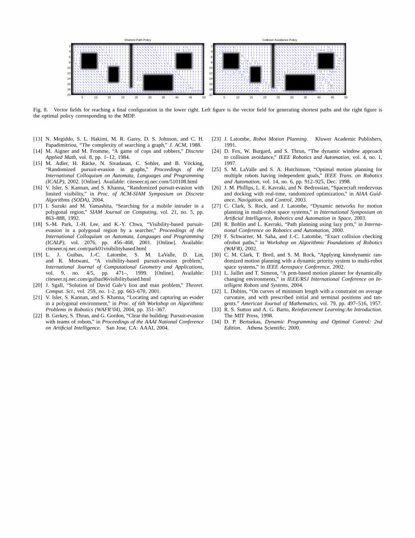
All other rewards and probabilities are zero. Once we buildthe MDP, we compute the optimal policy. In Figure 8, theoptimal collision avoiding policy for an arbitrary final state isdisplayed in contrast to the shortest-path policy.

C. Multi-robot settings

To explore the utility of the collision probabilities weperformed a simulation where our robot tries to reach afinal configuration amidstk = {1, . . . ,10} robots performinga random walk. For eachk, we performed 1000 experimentsand compared the success rate of the MDP optimal policywith the shortest path policy. The results are summarized inFigure 9.

0 2 4 6 8 10 120

0.1

0.2

0.3

0.4

0.5

0.6

0.7

0.8

0.9Success Rates

SPMDP

Fig. 9. Success rates in the presence ofk (horizontal axis) robots performinga random walk for the shortest path and optimal MDP policies.

V. CONCLUSION

In the recent years, roadmap based methods have beenextremely successful for motion-planning in complex configu-ration spaces. In this paper, we address two important roboticsproblems, pursuit-evasion and collision avoidance, and presentsolutions based on roadmaps.

In the first part of the paper, by using time aware controllersto build the roadmaps, we show how to obtain solutions tovarious pursuit-evasion games. The algorithms are based onthe dynamic programming (DP) principle and inherit bothadvantages and disadvantages of DP based approaches. Theprimary advantage is in the soundness and completeness ofthe algorithms. However, their running times increase withthedimension of the configuration space; making them practicalfor only low-dimensional configuration spaces. In our futurework, we plan to investigate this issue further.

In the second part of the paper, we presented a probabilisticframework for collision avoidance. We study a scenario wherethe robots react to each other only when they enter a certainreaction-zone. We assume that the robots are independent,however once they are within the reaction zone, they becomeunpredictable. To capture this unpredictability, we modelthemas adversarial pursuers and utilize the results from the firstpart to obtain worst-case guarantees for collision avoidance.This formulation allows us to process the workspace andbuild a collision-probability map. Afterwards, optimal colli-sion avoiding trajectories are computed using standard MDPalgorithms. Preliminary simulations demonstrate the utilityof our approach. In our future work, we plan to investigatethe effect of the diameter of the collision reaction zone andimplement the algorithm on real robots to further study theirfeasibility.

ACKNOWLEDGEMENTS

This work has been supported in part by NSF grants IIS-0438125 and EIA-0122599. We gratefully acknowledge theindustrial support through CITRIS organization.

REFERENCES

[1] J. Canny and J. Reif, “New lower bound techniques for robot motionplanning problems,” in28th Annual IEEE Symposium on Foundationsof Computer Science, 1987, pp. 49–60.

[2] S. M. LaValle, Planning Algorithms. [Online], 2004, available athttp://msl.cs.uiuc.edu/planning/.

[3] H. Choset and et. al.,Principles of Robot Motion: Theory, Algorithms,and Implementation. MIT Press, 2004.

[4] L. E. Kavraki, J.-C. Latombe, and R. Motwani, “Randomized queryprocessing in robot path planning,”Journal of Computer and SystemSciences, vol. 57, no. 1, pp. 50–60, August 1998.

[5] S. M. LaValle, M. S. Branicky, and S. R. Lindemann, “On the re-lationship between classical grid search and probabilistic roadmaps,”International Journal of Robotics Research, 2003.

[6] R. Isaacs,Differential Games. Dover, 1965.[7] T. Basar and G. J. Olsder,Dynamic Noncooperative Game Theory.

SIAM, 1998.[8] J. Hespanha, H. J. Kim, and S. Sastry, “Multiple-agent probabilistic

pursuit-evasion games,” inIn Proc. of the 38th Conf. on Decision andContr, 1999, pp. 2432–2437.

[9] R. Vidal, O. Shakernia, J. Kim, D. Shim, and S. Sastry, “Probabilisticpursuit-evasion games: Theory, implementation and experimental eval-uation,” IEEE Transactions on Robotics and Automation, vol. 18, pp.662–669, 2002.

[10] J. P. Hespanha, G. J. Pappas, and M. Prandini, “Greedy control forhybrid pursuit-evasion games,” inProceedings of the European ControlConference, Porto, Portugal, September 2001, pp. 2621–2626.

[11] R. Nowakawski and P. Winkler, “Vertex-to-vertex pursuit in a graph,”Discrete Math, vol. 43, pp. 235–239, 1983.

[12] T. D. Parsons, “Pursuit evasion in a graph,” inTheory and Applicationof Graphs, Y. Alavi and D. R. Lick, Eds. Springer Verlag, 1976, pp.426–441.

Shortest Path Policy

5 10 15 20 25 30 35 40 45 50

2

4

6

8

10

12

14

16

18

20

Collision Avoidance Policy

5 10 15 20 25 30 35 40 45 50

2

4

6

8

10

12

14

16

18

20

Fig. 8. Vector fields for reaching a final configuration in the lower right. Left figure is the vector field for generating shortest paths and the right figure isthe optimal policy corresponding to the MDP.

[13] N. Megiddo, S. L. Hakimi, M. R. Garey, D. S. Johnson, and C.H.Papadimitriou, “The complexity of searching a graph,”J. ACM, 1988.

[14] M. Aigner and M. Fromme, “A game of cops and robbers,”DiscreteApplied Math, vol. 8, pp. 1–12, 1984.

[15] M. Adler, H. Racke, N. Sivadasan, C. Sohler, and B. Vocking,“Randomized pursuit-evasion in graphs,”Proceedings of theInternational Colloquium on Automata, Languages and Programming(ICALP), 2002. [Online]. Available: citeseer.nj.nec.com/510108.html

[16] V. Isler, S. Kannan, and S. Khanna, “Randomized pursuit-evasion withlimited visibility,” in Proc. of ACM-SIAM Symposium on DiscreteAlgorithms (SODA), 2004.

[17] I. Suzuki and M. Yamashita, “Searching for a mobile intruder in apolygonal region,”SIAM Journal on Computing, vol. 21, no. 5, pp.863–888, 1992.

[18] S.-M. Park, J.-H. Lee, and K.-Y. Chwa, “Visibility-based pursuit-evasion in a polygonal region by a searcher,”Proceedings of theInternational Colloquium on Automata, Languages and Programming(ICALP), vol. 2076, pp. 456–468, 2001. [Online]. Available:citeseer.nj.nec.com/park01visibilitybased.html

[19] L. J. Guibas, J.-C. Latombe, S. M. LaValle, D. Lin,and R. Motwani, “A visibility-based pursuit-evasion problem,”International Journal of Computational Geometry and Applications,vol. 9, no. 4/5, pp. 471–, 1999. [Online]. Available:citeseer.nj.nec.com/guibas96visibilitybased.html

[20] J. Sgall, “Solution of David Gale’s lion and man problem,”Theoret.Comput. Sci., vol. 259, no. 1-2, pp. 663–670, 2001.

[21] V. Isler, S. Kannan, and S. Khanna, “Locating and capturing an evaderin a polygonal environment,” inProc. of 6th Workshop on AlgorithmicProblems in Robotics (WAFR’04), 2004, pp. 351–367.

[22] B. Gerkey, S. Thrun, and G. Gordon, “Clear the building:Pursuit-evasionwith teams of robots,” inProceedings of the AAAI National Conferenceon Artificial Intelligence. San Jose, CA: AAAI, 2004.

[23] J. Latombe,Robot Motion Planning. Kluwer Academic Publishers,1991.

[24] D. Fox, W. Burgard, and S. Thrun, “The dynamic window approachto collision avoidance,”IEEE Robotics and Automation, vol. 4, no. 1,1997.

[25] S. M. LaValle and S. A. Hutchinson, “Optimal motion planning formultiple robots having independent goals,”IEEE Trans. on Roboticsand Automation, vol. 14, no. 6, pp. 912–925, Dec. 1998.

[26] J. M. Phillips, L. E. Kavraki, and N. Bedrossian, “Spacecraft rendezvousand docking with real-time, randomized optimization,” inAIAA Guid-ance, Navigation, and Control, 2003.

[27] C. Clark, S. Rock, and J. Latombe, “Dynamic networks for motionplanning in multi-robot space systems,” inInternational Symposium onArtificial Intelligence, Robotics and Automation in Space, 2003.

[28] R. Bohlin and L. Kavraki, “Path planning using lazy prm,”in Interna-tional Conference on Robotics and Automation, 2000.

[29] F. Schwarzer, M. Saha, and J.-C. Latombe, “Exact collision checkingofrobot paths,” inWorkshop on Algorithmic Foundations of Robotics(WAFR), 2002.

[30] C. M. Clark, T. Bretl, and S. M. Rock, “Applying kinodynamic ran-domized motion planning with a dynamic priority system to multi-robotspace systems,” inIEEE Aerospace Conference, 2002.

[31] L. Jaillet and T. Simeon, “A prm-based motion planner for dynamicallychanging environments,” inIEEE/RSJ International Conference on In-telligent Robots and Systems, 2004.

[32] L. Dubins, “On curves of minimum length with a constraint on averagecurvature, and with prescribed initial and terminal positions and tan-gents.”American Journal of Mathematics, vol. 79, pp. 497–516, 1957.

[33] R. S. Sutton and A. G. Barto,Reinforcement Learning:An Introduction.The MIT Press, 1998.

[34] D. P. Bertsekas,Dynamic Programming and Optimal Control: 2ndEdition. Athena Scientific, 2000.