pure.york.ac.uk file · Web viewWord Count: 4,556 words Abstract . Distributional cost-effectiveness analysis (DCEA) is a framework for incorporating health inequality concerns into

Distributional Cost-Effectiveness Analysis

Title Page

Main title:

Distributional Cost-Effectiveness Analysis: A Tutorial

Running head:


Authors:

Miqdad Asaria1 (MSc), Susan Griffin1 (PhD) and Richard Cookson1 (PhD)

Centre for Health Economics, University of York

Financial Support:

The work was undertaken by the authors as part of the Public Health Research Consortium.

The Public Health Research Consortium is funded by the Department of Health Policy

Research Programme. The views expressed in the publication are those of the authors and

not necessarily those of the Department of Health. Information about the wider programme

of the PHRC is available from www.phrc.lshtm.ac.uk

Correspondence to:

Miqdad Asaria, Centre for Health Economics, University of York, York YO10 5DD, Tel: 01904

321973, Email: [email protected]

Word Count:

4,556 words

1 of 37

mailto:[email protected]


Abstract

Distributional cost-effectiveness analysis (DCEA) is a framework for incorporating health inequality

concerns into the economic evaluation of health sector interventions. In this tutorial we describe the

technical details of how to conduct DCEA, using an illustrative example comparing alternative ways

of implementing the NHS Bowel Cancer Screening Programme (BCSP). The two key stages in

DCEA are (A) modelling social distributions of health associated with different interventions and (B)

evaluating social distributions of health with respect to the dual objectives of improving total

population health and reducing unfair health inequality. As well as describing the technical methods

used, we also identify the data requirements and the social value judgements that have to be made.

Finally, we demonstrate the use of sensitivity analyses to explore the impacts of alternative modelling

assumptions and social value judgements.

Keywords

Cost-effectiveness analysis, economic evaluation, efficiency, equality, equity, fairness, health

distribution, health inequality, inequality measures, opportunity cost, social value judgements, social

welfare functions, trade-off

2 of 37


1. INTRODUCTION

When designing and prioritising interventions, health care decision makers often have concerns about

reducing unfair health inequality as well as improving total population health. However, the

economic evaluation of such interventions is typically conducted using methods of cost-effectiveness

analysis (CEA) which focus exclusively on maximising total population health. These standard

methods of CEA do not provide decision makers with information about the health inequality impacts

of the interventions evaluated, or the nature and size of any trade-offs between improving total

population health and reducing unfair health inequality.

To address these shortcomings we have developed a framework for incorporating health inequality

impacts into CEA, which we call “distributional cost-effectiveness analysis” (DCEA) (1). DCEA is

suitable for health sector decisions concerning the design and prioritisation of any type of health care

intervention with an explicit health inequality reduction objective – potentially including treatments as

well as preventive health care such as programmes of health promotion, screening, vaccination, case

finding, primary and secondary prevention of chronic disease, and so on. However, like standard

CEA, it focuses exclusively on health benefits and opportunity costs falling on the health sector

budget. DCEA therefore does not provide a fully general framework of distributional economic

evaluation for evaluating the health and income inequality impacts of cross-government public health

programmes with important non-health benefits and opportunity costs falling outside the health sector

budget.

The DCEA framework has two main stages: (A) modelling social distributions of health associated

with each intervention, and (B) evaluating social distributions of health. The main steps in the

modelling stage are:

A1. estimating the baseline health distribution;

A2. modelling changes to this baseline distribution due to the health interventions being

compared, allowing for the distribution of opportunity costs from additional resource

use;

3 of 37


A3. adjusting the resulting modelled health distributions for alternative social value

judgements about fair and unfair sources of health variation;

And the main steps in the evaluation stage are:

B1. using the estimated distributions to quantify the change in total population health and

unfair health inequality due to each intervention;

B2. ranking the interventions based on dominance criteria; and finally

B3. analysing any trade-offs between improving population health and reducing unfair

health inequality, allowing for alternative specifications of the underlying social

welfare function.

We have previously applied the DCEA framework to analyse four possible options for promoting

increased uptake of the NHS Bowel Cancer Screening Programme (BCSP) in England (2). In this

tutorial we work through this applied example to describe the key steps in conducting a DCEA.

The BCSP is a biennial self-test based screening programme targeted at 60-74 year olds that aims to

detect and treat colorectal cancer (CRC) early, and has been shown to reduce CRC related mortality

risk by a substantial proportion. Individuals in the relevant age range are sent a guaiac faecal occult

blood test (gFOBT) kit in the mail and are expected to complete the test by collecting 3 stool samples

over a period of a few days and post them back for laboratory analysis. Those individuals testing

positive are invited for further diagnostic testing (follow up colonoscopy) and, where appropriate,

treatment.

Analysis of the BCSP pilots and early data from the roll out of the BCSP have indicated large

variations in uptake of the screening programme patterned by the social variables of area deprivation,

sex and ethnicity. This variation in uptake can be modelled through to estimate its impact on

mortality and morbidity for the different socio-economic subgroups in the population, and hence to

describe the impact of the screening programme on both the average level of health and on the social

distribution of health in the population.

4 of 37


2. METHODS

2.1 Stage A: Modelling Social Distributions of Health

2.1.1 Estimating the baseline health distribution

The first step in DCEA is to describe the baseline distribution of health, taking into account variation

in both length and health related quality of life. This baseline distribution will need to include the full

general population, and not just the population of recipients of the intervention. This is for two

reasons. First, the full general population is typically the relevant population for characterising policy

concern with health inequality. Second, within the context of a national, budget constrained system

such as the NHS, additional resources used by recipients of an intervention will displace activities that

could have been provided to anyone within the full general population.

This baseline distribution of health should be able to describe variation in health among multiple

different subgroups in the population as defined by relevant population characteristics, allowing for

the correlation structure between these various characteristics. The relevant population characteristics

include not only dimensions of direct equity concern (e.g. income, ethnicity) but also characteristics

necessary to estimate expected costs and effects and which may or may not generate further equity

concern (e.g. sex). The latter of these is standard for any CEA, while the former we discuss further

throughout this tutorial. The health metric we use in this context is quality adjusted life expectancy

(QALE) at birth, though other suitable health metrics could also be used – such as disability adjusted

life expectancy at birth or age-specific QALE – so long as they are measured on an interpersonally

comparable ratio scale suitable for use within CEA.

The population characteristics of interest in this case study – those by which a substantial variation in

uptake of the BCSP was observed – are sex, area level deprivation and area level ethnic diversity.

The first step in estimating our population QALE distribution is to estimate life expectancy (LE)

according to each of these characteristics. Area level deprivation in the BCSP evaluation studies was

measured based on index of multiple deprivation (IMD 2004) quintile groups, and area level ethnic

diversity was based on the percentage of people in the area originating from the Indian Subcontinent,

5 of 37


again split into quintile groups (3). National statistics data are available by sex and deprivation

level/social class but are not available by our particular measure of ethnic diversity. We therefore did

not include correlations with ethnic diversity in our estimation of the baseline health distribution and

instead, for the purposes of the analysis, assumed its distribution is independent of deprivation and

sex.

A full description of how the baseline health distribution was calculated can be found in the appendix.

A summary of this QALE distribution by health quintile is shown in Figure 1. This forms the

baseline health distribution that we will use in our analysis.

FIGURE 1 approximately here

2.1.2 Estimating the distribution of health changes due to the interventions

In order to evaluate changes in the baseline health distribution that could be attributed to the use of

alternative interventions, it is necessary to know how the costs and effects of the intervention differ

between the relevant subgroups, and how the opportunity costs of any change in resource use differ by

those same subgroups.

Having estimated a baseline health distribution we next turn to modelling how this health distribution

is impacted by the BCSP and alternative ways of promoting increased uptake of the BCSP. We do

this using an existing cost-effectiveness model of the BCSP that simulates the natural history of CRC

and the impact of screening and treatment on this natural history (4)(5). We adapt the model to look

at the distributional health impacts of four different screening strategies:

I. “No Screening”: the baseline social distribution of health

II. “Standard Screening” as implemented in the BCSP

III. “Targeted reminder”: Screening plus a targeted enhanced reminder letter (personal GP signed

letter and tailored information package) sent only to those living in the most income deprived

small areas (IMD4 and IMD5) as well as to those living in areas with the highest proportion

of inhabitants from the Indian Subcontinent (IS5).

6 of 37


IV. “Universal reminder”: Screening plus a universal basic reminder letter (sending a GP

endorsed reminder letter to all eligible patients).

Impacts are first estimated by subgroup and then combined to evaluate the impact of the screening

strategies on the overall social distribution of health.

There are a number of parameters in the model that can vary by subgroup, including:

1. Disease prevalence, severity, mortality rate and natural history - we assume in our case study

that bowel cancer specific parameters are constant across our population subgroups. The

evidence available (6) broadly supports this assumption, though more detailed data at the

subgroup level would be required to validate this assumption.

2. Uptake of the intervention – the impact of gFOBT uptake by subgroup is the key difference

between the various implementations of the screening programme. We discuss in detail below

how this parameter is estimated for each subgroup. We also estimate the uptake of follow up

colonoscopy by subgroup for those people that are invited back for further investigation after

being screened.

3. Direct costs associated with the intervention - we assume the direct costs related to treating a

given stage of bowel cancer do not vary by subgroup (though the chance of incurring these

costs and the screening related costs by subgroup may vary under the different

implementations of the screening programme). This seems to be a plausible assumption in

the absence of more detailed cost data at the subgroup level.

4. Opportunity costs from displaced activities - Opportunity costs are in the base case analysis

assumed to be shared equally among all population subgroups, this assumption is explored in

sensitivity analyses discussed later in this tutorial.

5. Other cause mortality – we use the mortality rates by subgroup in the same way as discussed

when deriving the baseline health distribution. In calculating these rates we remove bowel

cancer specific mortality assuming this is constant across subgroups and apply this separately

in the model.

7 of 37


Quality adjustment of health gains to reflect morbidity – we apply the subgroup specific adjustments

to quality adjust health gains resulting from the screening programme in a similar manner to that

which they were applied to estimate the baseline health distribution. The population QALE

distribution under no screening corresponds to our baseline health distribution as calculated in the

previous section. In our analysis of the BCSP we include an additional variable – area level

proportion of population from the Indian Subcontinent (IS) – which we were unable to incorporate

into our estimation of the baseline health distribution. We assume that this IS variable is distributed

independently of IMD and sex, and that it has no independent effect on baseline QALE i.e. subgroups

are adjusted for other cause mortality and quality adjusted only according to their IMD and sex and

these adjustments are not effected by their IS. We next adjust the BCSP uptake parameters by

subgroup. Table I shows logistic regression results looking at gFOBT uptake in the three rounds of

the BCSP pilot (3). We use this data in combination with the proportion of invitees in each category

by variable, also reported in the pilot evaluation, to get weighted average odds ratios (OR) for uptake

that can be applied in the model.

TABLE I approximately here

These odds ratios are applied to a baseline rate of uptake reported in the third round pilot where

males in the youngest age group, living in the most deprived areas with the highest proportion of

people from the Indian subcontinent had an uptake probability of 34%. For example, to calculate the

uptake probability for a woman of any age across all rounds of the pilot, living in the least deprived

areas and with the least numbers of people from the Indian Subcontinent, we can use the following

calculation.

OR = 0.34/(1-0.34) * (1.38 /0.82) * 1.13 * 0.86 * (1/0.37) * (1/0.86) = 2.71

P = OR/(1+OR) = 0.73

A similar regression analysis was reported analysing the effect of these same variables on the uptake

of follow up colonoscopy. Data were also published in the pilot study evaluation regarding the

numbers of people in each category for each variable in the study. However, cross-tabulations or

8 of 37


correlations between the variables were not available and we therefore assumed that each variable was

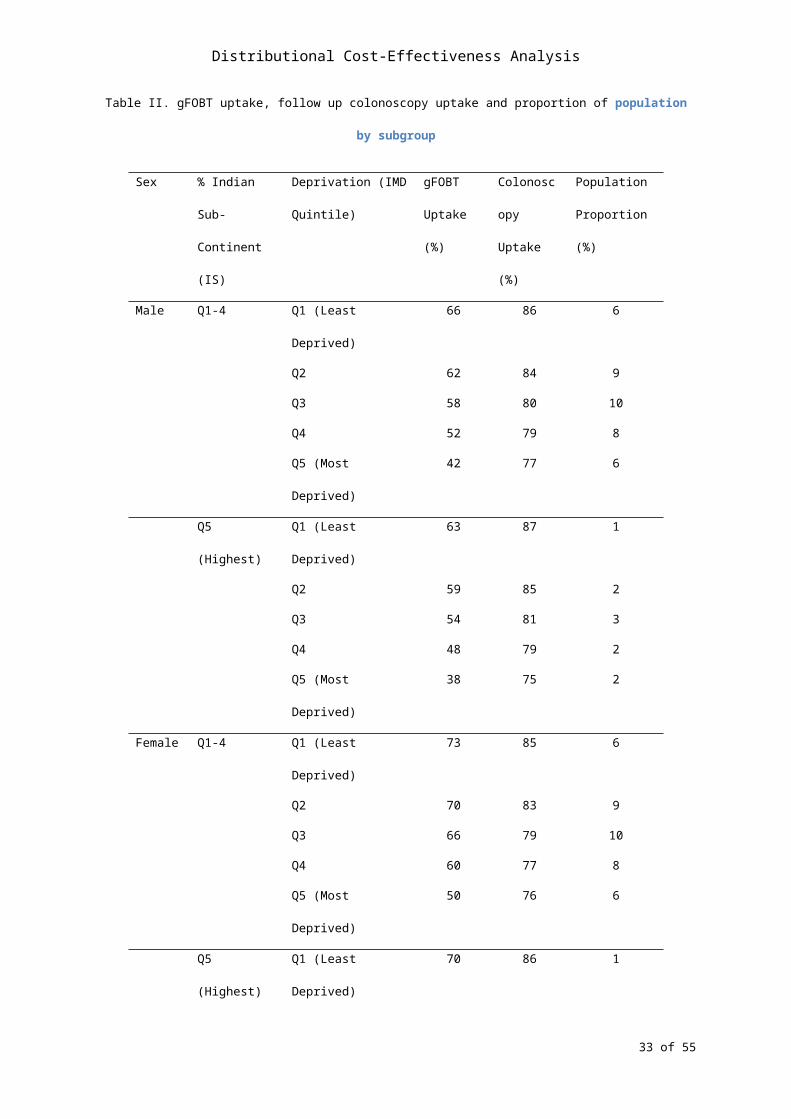
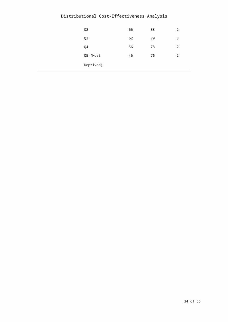
independently distributed to calculate the proportion of the population in each subgroup. Table II

shows our calculated gFOBT uptake, follow up colonoscopy uptake, and the proportion of the

population by each subgroup.

TABLE II approximately here

Using these parameters in the model provides the total costs and health gains due to the BCSP under

the standard screening approach.

We next turn to modelling the remaining two implementations of the screening programme. Both

implementations augment the standard screening programme with additional reminders. We derive

indicative estimates of costs and impacts on screening uptake of these reminder strategies from

similar interventions studied in the screening literature (7)(8), applying plausible exchange rates and

inflation rates to the figures to get costs and assuming all subgroups receiving the interventions have

equal additive increases in uptake. The values used in the model for costs and impacts on gFOBT

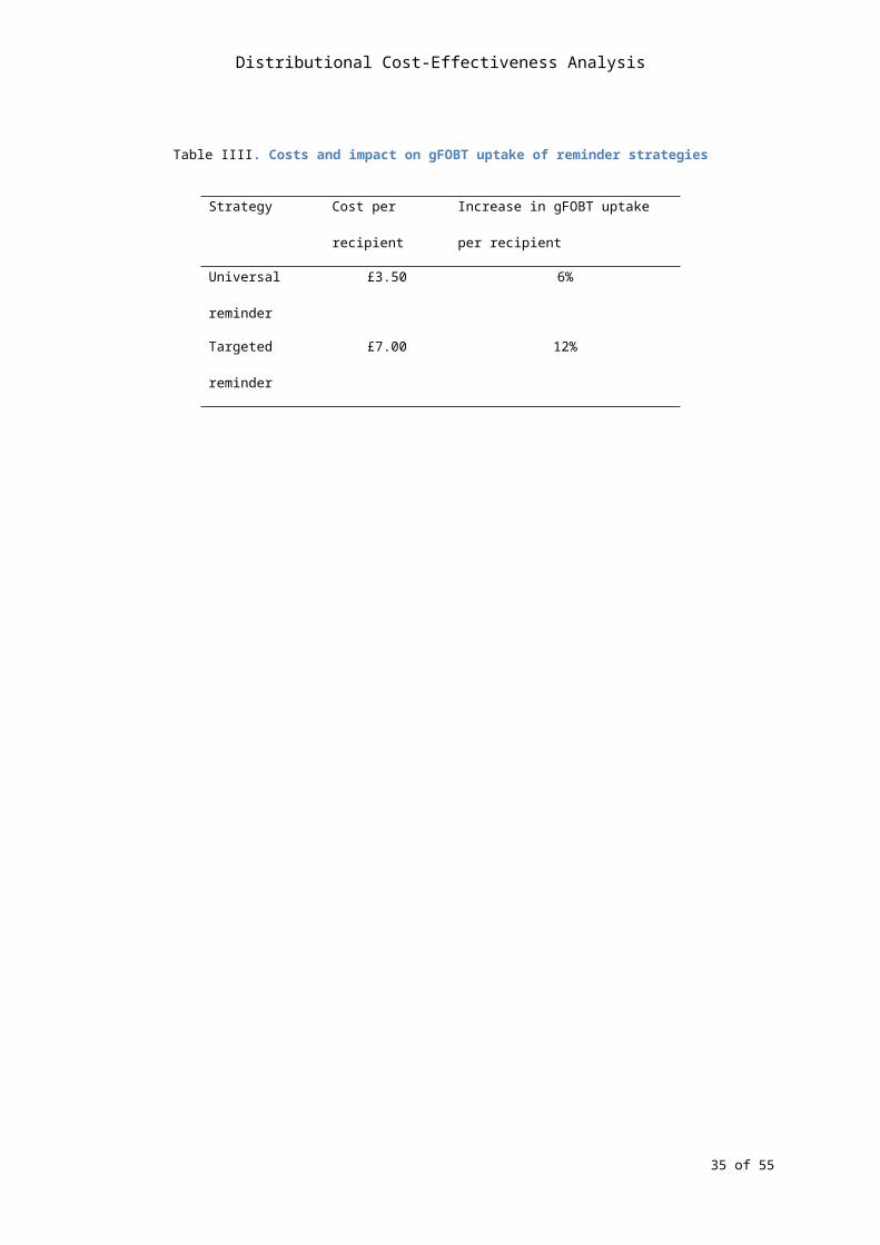
uptake for each of the strategies are given in Table III.

TABLE III approximately here

In order to estimate total costs and health effects the model is evaluated for a representative cohort of

the population – in our case a cohort of 1 million 30 year olds, as was used in the original analysis of

the BCSP in the model we inherited. The size of each subgroup is given by the population

proportions calculated in Table II. We sum the costs across all subgroups, and convert these to health

opportunity costs using a threshold value of £20,000 per QALY. These health opportunity costs are

then apportioned equally to each individual in the population allowing the model to characterise net

health gains in each subgroup. For example, the total costs for the standard screening programme

over the lifetime of the cohort of 1 million patients came to £72 million. Converting this to health

opportunity costs at the rate of £20,000 per QALY gives us 3,600 QALYs of health opportunity costs.

Women who live in areas with a low percentage of the population from the Indian Subcontinent (IS

9 of 37


Q1-4), and which also fall within deprivation quintile IMD Q3, make up 10% of the population. So

we allocate 10% of this total health opportunity cost to them i.e. 360 QALYs. This is then subtracted

from the total health gains due to the BCSP in this subgroup to give the net health effect of the BCSP

on this subgroup.

The assumption of equally distributed opportunity cost is convenient, but not evidence based. So we

explore alternative assumptions in sensitivity analysis, focusing on two extreme cases where all

opportunity costs are allocated to the least healthy and the healthiest subgroups, respectively.

The additional parameters that we have added to the model are assigned standard distributions by

variable type, and their mean and standard error values are used to generate suitable random draws for

these variables in the probabilistic sensitivity analysis (PSA). Details of how these additional

variables are dealt with in the PSA are given in Table V. All the results presented are produced by

running the model probabilistically and averaging over 1000 iterations of the model.

The resulting health distributions estimated for each screening implementation are described below.

Figure 2a shows the gFOBT uptake by health quintile for each strategy and Figure 2b shows the

colonoscopy uptake by health quintile. QALE for each subgroup calculated from our adjusted model

is given in Table IV and these are presented for our cohort by health quintile in Figure 3a and Figure

3b allowing us to better appreciate the relative impacts of the strategies.


TABLE IV approximately here


TABLE V approximately here

2.1.3 Adjusting for social value judgements about fair and unfair sources of inequality

The distributions of health estimated thus far represent all variation in health in the population.

However, some variation in health may be deemed “fair” or, at least “not unfair”, perhaps because it

10 of 37


is due to individual choice or unavoidable bad luck. In such cases the health distributions should first

be adjusted to only include health variation deemed “unfair” before measuring the level of inequality.

Social value judgements need to be made about whether or not health variation associated with each

of the population characteristics is deemed fair. In our example we have three variables to consider:

sex, IMD and ethnicity. We might make the value judgement that differences in health due to sex are

fair, while differences in health due to IMD and ethnicity are unfair – this is one of eight possible

value judgements that we can make on fairness in this example. One way of adjusting our modelled

health distributions for this value judgement is by using direct standardisation (9). To do this we run

a regression on our QALE distribution weighting the subgroups by the proportion of the population

they represent to find the association between each variable and QALE. An example of such a

regression is given in Table VI. We then use reference values for those variables deemed fair (i.e. sex

in this case) while leaving the other variables to take the values they have in the relevant subgroups

and predict out an adjusted QALE distribution. In this example we use male as the reference value for

sex and predict out the QALE distribution as shown in Table VII. This distribution represents only

the variation in health deemed unfair by the social value judgement made. Reference values used in

the adjustment process are typically population averages for continuous variables while for

categorical variables the most commonly occurring category is typically used with sensitivity analysis

performed on the impact of alternative choices of reference category.

TABLE VI approximately here

TABLE VII approximately here

2.2 Stage B: Evaluating Social Distributions of Health

2.2.1 Comparing interventions in terms of total health and unfair health inequality

Once we have estimated the appropriate health distributions we can then go on to characterise the

distributions in terms of the twin policy goals of improving total health and reducing health

inequality. One useful piece of information for decision makers produced at this step of the analysis

is the size of the health opportunity cost of choosing an intervention that reduces health inequality –

11 of 37


this is simply the difference in total health between the intervention and a comparator. However, this

step of the analysis can also go further than that by providing information about the size of the

reduction in health inequality, in terms of the difference in one or more suitable inequality indices

between the intervention and a comparator. The selection of appropriate inequality indices requires

further value judgements about the nature of the inequality concern. There are a number of

commonly used indices to measure inequality that can be broadly grouped into those measuring

relative inequality (scale invariant indices), those measuring absolute inequality (translation invariant)

and those measuring health poverty or shortfall from a reference value. If there is no clear choice of

inequality measure it may be preferable to calculate a range of alternative measures.

Table VIII shows the results of calculating a range of relative and absolute inequality measures for the

QALE distributions associated with our four screening strategies. A higher value for each measure

indicates a higher level of inequality between the most healthy and the least healthy.

TABLE VIII approximately here

2.2.2 Ranking interventions using dominance rules

The first step in comparing distributions is looking to commonly used distributional dominance rules,

as these allow strategies to be ranked with minimal restriction to the form of the underlying social

welfare function. In terms of standard economic dominance rules we can note from Table IV that no-

screening and standard screening are strictly dominated in the space of QALE by the universal

reminder strategy – that is, no sex-IMD-ethnicity subgroup is less healthy and at least one subgroup is

healthier. However, this rule does not account for the level of inequality. When ranking distributions

based on mean health and the level of health inequality, it is possible to use alternative economic

dominance rules provided by Atkinson (10) and Shorrocks (11). These dominance rules apply when

mean health is higher and inequality is lower for almost any measure of inequality. Both rules are

based around the Lorenz curve (12), a tool to analyse relative inequality constructed for health

distributions by ordering the population from least healthy to most healthy and plotting the cumulative

proportion of population health against the cumulative proportion of the population. Atkinson’s

12 of 37


theorem tests for Lorenz dominance between distributions; this means that the Lorenz curves for the

distributions do not cross and the more equal distribution has at least as much mean health as the less

equal distribution. In other words, a distribution is dominated if it has higher inequality and the same

or lower amount of mean health. On these criteria the standard screening strategy is dominated by the

targeted reminder. Shorrocks’ theorem tests for generalised Lorenz dominance, wherein the Lorenz

curve is multiplied by the mean health. A distribution is dominated if the generalised Lorenz curve

lies wholly below that of an alternative intervention. Under this criterion, both the targeted and

universal reminder strategies dominate the no screening option. This leaves us to compare the

universal reminder and targeted reminder strategies. While the universal reminder produces a higher

average QALE overall and benefits the less deprived quintile groups more, the targeted reminder is

the more equal strategy on every measure listed in Table VIII and benefits the most deprived quintile

groups more. In our example, the generalised Lorenz curves for these two distributions cross and

hence we cannot use Shorrocks’ theorem to rank the distributions.

2.2.3 Analysing trade-offs between total health and health inequality using social welfare indices

Having used distributional dominance to eliminate no screening and standard screening, in order to

rank the remaining two strategies it is necessary more fully to specify an underlying social welfare

function. A number of alternative social welfare indices have been proposed that could be used to

characterise the dual objectives of increasing total health and reducing health inequality. A common

feature of such functions is the need to specify the nature of and level (or value) of inequality

aversion. The inequality aversion parameters in these functions describe the trade-off between total

health and the level of health inequality, i.e. the amount of total health that a decision maker would be

willing to sacrifice in order to achieve a more equal distribution. These inequality aversion

parameters are difficult to interpret on the raw scale. A more intuitive scale can be provided by

combining a specific value of the parameter with a specific health distribution to derive the “equally

distributed equivalent” (EDE) level of health. The difference between the mean level of health in that

distribution and the EDE level of health then represents the average amount of health per person that

13 of 37


one would be willing to sacrifice to achieve full equality in health, given that specific value of

inequality aversion.

In this example we will use two social welfare indices closely linked to the dominance rules applied

above: the Atkinson index (10) to evaluate the distributions in terms of relative inequality and the

Kolm index (13) to evaluate the distributions in terms of absolute inequality. The EDE for these

social welfare indices can be calculated as follows using the inequality aversion parameters ɛ and α

respectively:

Atkinson Social Welfare Index: Kolm Social Welfare Index:

Figure 4a and Figure 4b show the difference in EDE health between the two strategies across different

levels of inequality aversion for the relative and absolute social welfare indices respectively. With

zero inequality aversion the EDE represents the mean health, and we see that the universal strategy

offers 1,000 more population QALYs compared to the targeted strategy. For inequality aversion

levels greater than ɛ =8 and α =0.12 the targeted strategy would be preferred, implying that the

decision maker would be willing to sacrifice those 1,000 population QALYs in order to achieve the

lower level of inequality.


Recent work on eliciting these inequality aversion parameters from members of the general public in

England (14) estimates an Atkinson ɛ parameter of about 10.95 (95% CI: 9.23-13.54) and a Kolm α

parameter of about 0.15 (95% CI: 0.13-0.19).

2.3 Sensitivity analysis

There are a number of sensitivity analyses we can run to explore the impact of making alternative

assumptions in our modelling on our choice of preferred strategy. Tables IX and X present the

14 of 37


results, respectively, of exploring (1) the impacts of alternative assumptions around the distribution of

opportunity costs, and (2) the impacts of alternative social value judgements about which inequalities

are considered unfair.

TABLE IX approximately here

TABLE X approximately here

We could also perform additional sensitivity analyses including exploring alternative ways that the

reminder strategies might affect the different population subgroups e.g. having constant proportional

effects rather than constant absolute effects and testing for alternative underlying distributions of CRC

mortality, incidence and severity.

3. DISCUSSION

DCEA is a framework for incorporating health inequality concerns into the cost-effectiveness analysis

of health care interventions. It aims to help cost-effectiveness analysts provide decision makers with

useful quantitative information about the health inequality impacts of health care interventions, and

the nature and size of trade-offs between the dual objectives of improving total health and reducing

health inequality. It also aims to help cost-effectiveness analysts accommodate different value

judgements about health inequality made by different decision makers and stakeholders.

Social value judgements about health inequality are complex, context-dependent and contestable. For

this reason, DCEA does not prescribe in advance any particular set of social value judgements about

health inequality. A number of social value judgements need to be made when implementing the

DCEA framework, in particular regarding which dimensions of inequality are deemed unfair and the

nature and strength of inequality aversion. The framework makes these social value judgements

explicit and transparent, and lends itself well to checking the sensitivity of conclusions based upon

alternative plausible social value judgements. DCEA thus aims to provide decision makers with

useful quantitative information about health inequality impacts that can help to inform a deliberative

decision making process, by showing how different social value judgements might or might not lead

15 of 37


to different conclusions. Empirical work to estimate the nature and level of societal inequality

aversion implicit in current healthcare allocation decisions would be useful in validating and

complementing estimates of the inequality aversion levels emerging from value elicitation exercises

conducted on members of the general public in England (14). This work would be analogous to the

recent work that has been done to generate empirical estimates of the cost-effectiveness threshold

(15).

DCEA is intended to be general and flexible analytical framework that allows a diverse range of

specific methods and techniques to be applied at different stages of the analysis. In particular, the

evaluation stage can in principle employ any kind of equity weighting and/or multi-criteria decision

analysis to analyse trade-offs between improving total health and reducing health inequality, and is

not restricted to application of the specific Atkinson and Kolm social welfare functions described in

this tutorial.

We have seen in this tutorial that DCEA is demanding in terms of data, but feasible to implement in a

real world context through creative application of the standard tools of economic analysis. The data

and methods we have used are inevitably partial and crude in many respects, and it is our hope that

the underpinning data and technical methods will be improved and refined over the years. Whilst the

framework and methods involved may seem complex, in our opinion this complexity is well within

the capabilities of analysts currently conducting standard CEA. The key to expanding the use of

DCEA will be the development of better methods for assisting decision-makers to clarify and quantify

the nature of their inequality concerns, and better ways of communicating findings to non-specialist

audiences.

16 of 37


APPENDIX

Estimating the baseline health distribution

Data on LE by IMD quintile and sex is published directly by the Office of National Statistics (16).

However, for the purposes of our analysis we also require the underlying mortality rates used to

estimate these figures in order to incorporate them in the decision analytical model where all-cause

mortality is separated from colorectal cancer specific mortality. Unfortunately, these underlying

mortality rates are not available by IMD quintile groups. So to ensure we remain consistent between

our baseline QALE distribution and QALE distributions associated with the various implementations

of the BCSP produced by our model, we use ONS mortality rates by social class (17) to proxy those

by IMD, and apply the mapping between social classes and IMD quintile groups given in Table A.I.

TABLE A.I approximately here

We then use these mapped mortality rates to calculate the LE at birth by IMD quintile groups (2002-

05) using the standard ONS methodology (18). Table A.II compares life expectancies estimated

indirectly using the mapping process described above with published direct estimates of life

expectancy by IMD quintile for the same period (2002-05). We see from the comparison that while

the mapped values are on the whole reasonably close to the published values, they begin to diverge

for the more deprived areas.

TABLE A.II approximately here

We next adjust these life expectancies for morbidity. To do this we adjust for age and sex by

applying the relevant weights from the published EQ-5D Norms (19) for each age range (reproduced

in Table A.III) and aggregate to give and age and sex adjusted QALE. Taking the example of a male

in the least deprived IMD quintile group (Q1) we can read from Table A.II that their estimated life

expectancy is 80.4 years. Using the weights in Table A.III we estimate the QALE for individuals in

this subgroup as:

17 of 37


24*0.94 + (35-25)*0.93 + (45-35)*0.91 + (55-45)*0.84 + (65-55)*0.78 + (75-65)* 0.78 + (80.5-75)*0.75 = 69.8 QALYs

TABLE A.III approximately here

In addition to quality adjusting LE for age and sex, we also would like to adjust for variation in

quality of life by area level deprivation. In order to do this we turn to the ONS data for LE and

disability free life expectancy (DFLE) by IMD quintile (16). We assume that the average quality

adjustment we have applied by using the age and sex weights captures the adjustment for the middle

IMD quintile group (Q3)for each sex, and calculate relative adjustment factors for the other IMD

quintile groups by further assuming the ratio of DFLE to LE is the same as the ratio of QALE to LE.

We use this data to calculate the adjustment factors shown in Table A.IV.

TABLE A.IV approximately here

Applying the adjustment factor to our QALE estimate for our male from IMD Q1 gives a refined

QALE estimate taking into account area level deprivation of:

69.8 * 1.03 = 72 QALYs

Similar calculations for the other subgroups yield the QALE estimates in Table A.V.

TABLE A.V approximately here

Ordering the subgroups by QALE from least healthy to most healthy and adjusting for the size of each

subgroup we are able to create a population distribution of QALE at birth taking into account

differential mortality and morbidity by age, sex and area level deprivation.

18 of 37


TABLES

Table I. Regression results of gFOBT uptake from evaluation of BCSP pilot

Adjusted OR

(95% CI)

Age (years) 57-59 1

60-64 1.13

(1.11 – 1.16)

65-69 1.25

(1.22 – 1.28)

Sex Male 1

Female 1.38

(1.35 – 1.40)

Pilot Round 1 1

2 0.77

(0.76 – 0.80)

3 0.82

(0.81 – 0.84)

Deprivation Category

(IMD)

Q1 (Least Deprived) 1

Q2 0.84

(0.81 -0.87)

Q3 0.70

(0.68 – 0.72)

Q4 0.55

(0.54 – 0.57)

Q5 (Most Deprived) 0.37

(0.35 – 0.38)

% Indian Subcontinent Q1-4 1

Q5 (Highest %) 0.86

(0.84 – 0.89)

19 of 37


Table II. gFOBT uptake, follow up colonoscopy uptake and proportion of population by subgroup

Sex % Indian Sub-

Continent (IS)

Deprivation (IMD

Quintile)

gFOBT

Uptake (%)

Colonoscopy

Uptake (%)

Population

Proportion (%)

Male Q1-4 Q1 (Least Deprived) 66 86 6

Q2 62 84 9

Q3 58 80 10

Q4 52 79 8

Q5 (Most Deprived) 42 77 6

Q5 (Highest) Q1 (Least Deprived) 63 87 1

Q2 59 85 2

Q3 54 81 3

Q4 48 79 2


Female Q1-4 Q1 (Least Deprived) 73 85 6

Q2 70 83 9

Q3 66 79 10

Q4 60 77 8


Q5 (Highest) Q1 (Least Deprived) 70 86 1

Q2 66 83 2

Q3 62 79 3

Q4 56 78 2


20 of 37


Table IIII. Costs and impact on gFOBT uptake of reminder strategies

Strategy Cost per recipient Increase in gFOBT uptake per recipient

Universal reminder £3.50 6%

Targeted reminder £7.00 12%

21 of 37


Table IV. QALE distribution by subgroup under each strategy

QALE

Sex % Indian Sub-

Continent (IS)

Deprivation (IMD

Quintile) Baseline Standard Targeted Universal

Male Q1-4 Q1 (Least Deprived) 72.16 72.21 72.20 72.21

Q2 70.48 70.52 70.52 70.52

Q3 69.09 69.12 69.12 69.13

Q4 66.61 66.63 66.63 66.63

Q5 (Most Deprived) 60.22 60.24 60.24 60.24

Q5 (Highest) Q1 (Least Deprived) 72.16 72.20 72.21 72.21

Q2 70.48 70.52 70.52 70.52

Q3 69.09 69.12 69.13 69.12

Q4 66.61 66.63 66.63 66.63

Q5 (Most Deprived) 60.22 60.23 60.24 60.23

Female Q1-4 Q1 (Least Deprived) 74.84 74.91 74.91 74.92

Q2 73.10 73.16 73.16 73.17

Q3 71.77 71.82 71.81 71.82

Q4 69.19 69.23 69.24 69.23

Q5 (Most Deprived) 63.17 63.20 63.20 63.20

Q5 (Highest) Q1 (Least Deprived) 74.84 74.91 74.92 74.91

Q2 73.10 73.16 73.17 73.16

Q3 71.77 71.81 71.82 71.82

Q4 69.19 69.23 69.24 69.23

Q5 (Most Deprived) 63.17 63.20 63.20 63.20

Overall

Average69.260 69.300 69.301 69.302

22 of 37


Table V. Distributions and parameter values used in PSA for additional parameters added to model

Parameter Explanation

gFOBT and colonoscopy

uptake

Uncertainty on these calculated in PSA assuming ln(OR) distributed normally. The

variance covariance matrices for the uptake regressions were not available to us so we

drew each coefficient independently and combined to create uptake probabilities.

Mortality rates Adjusted for uncertainty by the underlying model.

Quality adjustment Used beta distribution with the mean and standard error values as reported in the UK

EQ-5D norms.

Cost of reminders As no data was given on the uncertainty we assume a 10% standard error and used

this to draw values from the appropriate gamma distributions.

Impact of reminders on

uptake

Reported mean and standard errors values used to draw from the appropriate beta

distributions.

23 of 37


TableVI. Fairness adjustment regression

Coefficient

(SE)

Constant74.92

(4.37E-05)

IS Q1-4 -0.004

(2.56E-05)

Male-2.708

(5.47E-05)

IMD Q2-1.75

(4.91E-05)

IMD Q3-3.097

(4.84E-05)

IMD Q4-5.675

(5.02E-05)

IMD Q5-11.71

(5.33E-05)

Male*IMD Q20.065

(6.95E-05)

Male*IMD Q30.015

(6.84E-05)

Male*IMD Q40.104

(7.10E-05)

Male*IMD Q5-0.259

(7.532E-05)

24 of 37


TableVII. Fairness adjusted health distribution reference sex = male

QALE

Sex % Indian Sub-

Continent (IS)

Deprivation (IMD

Quintile) Targeted

Targeted

Adjusted

Male Q1-4 Q1 (Least Deprived) 72.20 72.20

Q2 70.52 70.52

Q3 69.12 69.12

Q4 66.63 66.63

Q5 (Most Deprived) 60.24 60.24

Q5 (Highest) Q1 (Least Deprived) 72.21 72.21

Q2 70.52 70.52

Q3 69.13 69.13

Q4 66.63 66.63


Female Q1-4 Q1 (Least Deprived) 74.91 72.20

Q2 73.16 70.52

Q3 71.81 69.12

Q4 69.24 66.63


Q5 (Highest) Q1 (Least Deprived) 74.92 72.21

Q2 73.17 70.52

Q3 71.82 69.13

Q4 69.24 66.63


25 of 37


Table VIII. Inequality measures calculated for four screening strategies

Relative Inequality Indices no screening standardtargeted

reminder

universal

reminder

Relative Gap Index (ratio) 0.17527* 0.17592 0.17586 0.17596

Relative Index of Inequality (RII) 0.18607* 0.18674 0.18668 0.18678

Gini Index 0.03101* 0.03112 0.03111 0.03113

Atkinson Index (ε=1) 0.00171* 0.00172 0.00172 0.00172

Atkinson Index (ε=7) 0.01330* 0.01337 0.01337 0.01338

Atkinson Index (ε=30) 0.06253* 0.06281 0.06279 0.06283

Absolute Inequality Indices no screening standardtargeted

reminder

universal

reminder

Absolute Gap Index (range) 10.98604* 11.03064 11.02726 11.03325

Slope index of inequality (SII) 12.88747* 12.94123 12.93691 12.94438

Kolm Index (α=0.025) 0.20281* 0.20430 0.20416 0.20439

Kolm Index (α=0.1) 0.87801* 0.88429 0.88371 0.88467

Kolm Index (α=0.5) 4.56391* 4.58739 4.58587 4.58883

* indicates the most equal strategy

ε=1 represents low relative inequality aversion while ε=30 represents high relative inequality aversion

α=0.025 represents low absolute inequality aversion while α=0.5 represents high absolute inequality aversion

26 of 37


Table IX. Sensitivity to alternative opportunity cost distributions

All opportunity cost borne by

least healthy subgroup

All opportunity cost borne by

healthiest subgroup

Social Welfare

Indicesno screening standard

targeted

reminder

universal

reminder

targeted

reminder

universal

reminder

Mean Health 69.25969 69.30006 69.30127 69.30233* 69.30127 69.30233*

Atkinson EDE

(ε=1) 69.14152 69.18056 69.18147 69.18252* 69.18286 69.18373*

Atkinson EDE

(ε=7) 68.33888 68.36800* 68.36610 68.36734 68.37799* 68.37769

Atkinson EDE

(ε=30) 64.92865* 64.91468 64.89302 64.89892 64.95627* 64.95350

Kolm EDE

(α=0.025) 69.05688 69.09486 69.09556 69.09660* 69.09793 69.09866*

Kolm EDE (α=0.1) 68.38168 68.41112* 68.40958 68.41074 68.42046* 68.42020

Kolm EDE (α=0.5) 64.69578* 64.68086 64.65951 64.66532 64.72148* 64.71879

* indicates the strategy yielding the highest social welfare

27 of 37


Table X. Sensitivity to alternative social value judgements

Social Value Judgment Preferred Strategy based on Social Welfare Index

IMD

Ethnic

Diversity Sex

Atkinson

EDE

(ε=1)

Atkinson

EDE

(ε=7)

Atkinson

EDE

(ε=30)

Kolm

EDE

(α=0.025)

Kolm EDE

(α=0.1)

Kolm EDE

(α=0.5)

Fair Fair Fair U U U U U U

Fair Unfair Fair U U U U U U

Fair Fair Unfair U U U U U U

Fair Unfair Unfair U U U U U U

Unfair Fair Fair U U T U U T

Unfair Unfair Fair U U T U U T

Unfair Fair Unfair U U T U U T

Unfair Unfair Unfair U U T U U T

U = universal reminder, T = targeted reminder

28 of 37


Table A.II. Mapping between IMD quintile groups and social class

Deprivation (IMD Quintile) Social Class

Q1 (Least Deprived) I&II (Professional occupations & Managerial and technical occupations)

Q2 I&II (Professional occupations & Managerial and technical occupations)

Q3 IIIN (Skilled non-manual occupations)

Q4 IIIM (Skilled manual occupations)

Q5 (Most Deprived) IV&V (Partly-skilled occupations & Unskilled Occupations)

29 of 37


Table A.III. Comparison between mapped and published LE by IMD quintile group

Sex

Deprivation (IMD

Quintile)

LE by Mapped IMD

Quintiles (years)

LE Published IMD Quintiles

(years)

Difference

(Mapped – Published)

Male Q1 (Least Deprived) 80.4 80.0 0.4

Q2 80.4 78.6 1.8

Q3 79.2 77.3 1.9

Q4 77.7 75.4 2.3

Q5 (Most Deprived) 76.2 72.2 4.0

Female Q1 (Least Deprived) 83.7 83.2 0.5

Q2 83.7 82.3 1.4

Q3 82.6 81.5 1.1

Q4 81.1 80.1 1.0

Q5 (Most Deprived) 80.3 77.9 2.4

30 of 37


Table A.IV. QALY weights by age and sex based on EQ-5D norms

Age Male Female

0-25 0.94 0.94

25-34 0.93 0.93

35-44 0.91 0.91

45-54 0.84 0.85

55-64 0.78 0.81

65-74 0.78 0.78

75+ 0.75 0.71

31 of 37


Table A.V. Using LE and DFLE to calculate QALE adjustment factors by IMD

Sex

Deprivation (IMD

Quintile) LE DFLE Ratio DFLE/LE

QALE Adjustment

Factor

Male Q1 (Least Deprived) 80.0 67.3 0.84 1.03

Q2 78.6 64.3 0.82 1.00

Q3 77.3 63.4 0.82 1.00

Q4 75.4 59.7 0.79 0.96

Q5 (Most Deprived) 72.2 54.2 0.75 0.91

Female Q1 (Least Deprived) 83.2 67.8 0.81 1.02

Q2 82.3 65.7 0.80 1.00

Q3 81.5 64.9 0.80 1.00

Q4 80.1 61.8 0.77 0.97

Q5 (Most Deprived) 77.9 57.2 0.73 0.92

32 of 37


Table A.VI. QALE by sex and deprivation

Sex Deprivation (IMD Quintile) QALE

Male Q1 (Least Deprived) 72.2

Q2 70.5

Q3 69.1

Q4 66.6


Female Q1 (Least Deprived) 74.8

Q2 73.1

Q3 71.8

Q4 69.2


33 of 37


FIGURES

Figure 1: Baseline health distribution

Figure 2a: gFOBT uptake distribution by strategy Figure 2b: colonoscopy uptake distribution

Figure 3a: Health compared to no screening (per million of

population invited for screened)

Figure 3b: Health compared to standard screening (per million of

population invited for screening)

34 of 37


Figure 4a: Sensitivity to level of relative inequality aversion

Figure 4b: Sensitivity to level of absolute inequality aversion

35 of 37


REFERENCES

1. Asaria M, Cookson R, Griffin S. Incorporating health inequality impacts into cost-effectiveness analysis. In: Culyer A, editor. Encyclopedia of Health Economics. San Diego: Elsevier; 2014. p. 22–6.

2. Asaria M, Griffin S, Cookson R, Whyte S, Tappenden P. Distributional Cost-Effectiveness Analysis of Health Care Programmes - a Methodological Case Study of the Uk Bowel Cancer Screening Programme. Health Econ [Internet]. 2014 May 2; Available from: http://www.ncbi.nlm.nih.gov/pubmed/24798212

3. Weller D. Evaluation of the 3rd Round of the English bowel cancer screening Pilot Report to the NHS Cancer Screening Programmes [Internet]. 2009. Available from: http://www.cancerscreening.nhs.uk/bowel/pilot-3rd-round-evaluation.pdf

4. Whyte S, Stevens J. Re-appraisal of the options for colorectal cancer screening Report for the NHS Bowel Cancer Screening Programme. 2011;1–61. Available from: http://www.cancerscreening.nhs.uk/bowel/scharr-full-report-summary-201202.pdf

5. Tappenden P, Chilcott J, Eggington S, Patnick J, Sakai H, Karnon J. Option appraisal of population-based colorectal cancer screening programmes in England. Gut [Internet]. 2007 May [cited 2012 Sep 18];56(5):677–84. Available from: http://www.pubmedcentral.nih.gov/articlerender.fcgi?artid=1942136&tool=pmcentrez&rendertype=abstract

6. National Cancer Intelligence Network. Cancer Incidence by Deprivation, 1995-2004 [Internet]. 2004 p. 1995–2004. Available from: http://www.ncin.org.uk/view.aspx?rid=73

7. Shankaran V, McKoy JM, Dandade N, Nonzee N, Tigue C a, Bennett CL, et al. Costs and cost-effectiveness of a low-intensity patient-directed intervention to promote colorectal cancer screening. J Clin Oncol [Internet]. 2007 Nov 20 [cited 2012 Oct 30];25(33):5248–53. Available from: http://www.ncbi.nlm.nih.gov/pubmed/18024871

8. Hewitson P, Ward a M, Heneghan C, Halloran SP, Mant D. Primary care endorsement letter and a patient leaflet to improve participation in colorectal cancer screening: results of a factorial randomised trial. Br J Cancer [Internet]. Nature Publishing Group; 2011 Aug 9 [cited 2012 Sep 6];105(4):475–80. Available from: http://www.pubmedcentral.nih.gov/articlerender.fcgi?artid=3170960&tool=pmcentrez&rendertype=abstract

9. Fleurbaey M, Schokkaert E. Unfair inequalities in health and health care. J Health Econ [Internet]. 2009 Jan [cited 2010 Nov 15];28(1):73–90. Available from: http://www.ncbi.nlm.nih.gov/pubmed/18829124

10. Atkinson AB. On the measurement of inequality. J Econ Theory [Internet]. 1970 [cited 2011 Jul 27];2(3):244–63. Available from: http://faculty.ucr.edu/~jorgea/econ261/atkinson_inequality.pdf

11. Shorrocks AF. Ranking Income Distributions. Economica [Internet]. 1983 Feb;50(197):3. Available from: http://links.jstor.org/sici?sici=0013-0427(198302)2:50:197<3:RID>2.0.CO;2-I&origin=crossref

36 of 37


12. Lorenz MO. Methods of Measuring the Concentration of Wealth. Publ Am Stat Assoc. 1905;9(70):209–12.

13. Kolm S-C. Unequal inequalities. I. J Econ Theory [Internet]. 1976 Jun;12(3):416–42. Available from: http://linkinghub.elsevier.com/retrieve/pii/0022053176900375

14. Matthew R, Asaria M, Cookson R, Ali S, Tsuchiya A. A066: Estimating the Level of Health Inequality Aversion in England. HESG Leeds Discuss Pap. 2015;

15. Claxton K, Martin S, Soares M, Rice N, Spackman E, Hinde S, et al. Methods for the Estimation of the NICE Cost Effectiveness Threshold. CHE Res Pap 81 [Internet]. 2013; Available from: http://www.york.ac.uk/media/che/documents/reports/resubmitted_report.pdf

16. ONS. Inequalities in disability-free life expectancy by area deprivation: England, 2001-04 to 2007-10 [Internet]. 2013. Available from: http://www.ons.gov.uk/ons/rel/disability-and-health-measurement/sub-national-health-expectancies/inequality-in-disability-free-life-expectancy-by-area-deprivation--england--2003-06-and-2007-10/rft-inequalities-in-disability.xls

17. ONS. Longitudinal Study age-specific mortality data 1972-2005 (supplementary tables) [Internet]. 2007. Available from: http://www.ons.gov.uk/ons/rel/health-ineq/health-inequalities/trends-in-life-expectancy-by-social-class-1972-2005/longitudinal-study-age-specific-mortality-data-1972-2005--supplementary-tables-.xls

18. Johnson B, Blackwell L. Review of methods for estimating life expectancy by social class using the ONS Longitudinal Study. 2007 p. 28–36.

19. Kind P, Hardman G, Macran S. UK population norms for EQ-5D [Internet]. 1999 [cited 2012 Oct 31]. Available from: http://www.york.ac.uk/media/che/documents/papers/discussionpapers/CHE Discussion Paper 172.pdf

37 of 37

Documents

pure.york.ac.uk file · Web viewWord Count: 4,556 words Abstract . Distributional cost-effectiveness analysis (DCEA) is a framework for incorporating health inequality concerns into