Embed Size (px)
Citation preview

TECHNICAL GUIDANCE MANUAL FOR HYDROGEOLOGICINVESTIGATIONS AND GROUND WATER MONITORING
CHAPTER 4SLUG AND PUMPING TESTS
February 1995
-ii-
TABLE OF CONTENTS
SINGLE WELL TESTS . . . . . . . . . . . . . . . . . . . . . . . . . . . . . . . . . . . . . . . . . . . . . . . . . . . . . . . . . . . 4-1SLUG TESTS . . . . . . . . . . . . . . . . . . . . . . . . . . . . . . . . . . . . . . . . . . . . . . . . . . . . . . . . . . . . . . . . 4-1
Design of Well . . . . . . . . . . . . . . . . . . . . . . . . . . . . . . . . . . . . . . . . . . . . . . . . . . . . . . . . . . . . 4-2Number of Tests . . . . . . . . . . . . . . . . . . . . . . . . . . . . . . . . . . . . . . . . . . . . . . . . . . . . . . . . . . . 4-2Test Performance and Data Collection . . . . . . . . . . . . . . . . . . . . . . . . . . . . . . . . . . . . . . . . 4-2Modified Slug Tests . . . . . . . . . . . . . . . . . . . . . . . . . . . . . . . . . . . . . . . . . . . . . . . . . . . . . . . . 4-2
Packer Tests Within A Stable Borehole . . . . . . . . . . . . . . . . . . . . . . . . . . . . . . . . . . . . 4-3Pressure Tests . . . . . . . . . . . . . . . . . . . . . . . . . . . . . . . . . . . . . . . . . . . . . . . . . . . . . . . . 4-3Vacuum Tests . . . . . . . . . . . . . . . . . . . . . . . . . . . . . . . . . . . . . . . . . . . . . . . . . . . . . . . . . . 4-4
Analysis of Slug Test Data . . . . . . . . . . . . . . . . . . . . . . . . . . . . . . . . . . . . . . . . . . . . . . . . . . 4-6SINGLE WELL PUMPING TESTS . . . . . . . . . . . . . . . . . . . . . . . . . . . . . . . . . . . . . . . . . . . . . . . 4-6
MULTIPLE WELL PUMPING TESTS . . . . . . . . . . . . . . . . . . . . . . . . . . . . . . . . . . . . . . . . . . . . . . . 4-9PRELIMINARY STUDIES . . . . . . . . . . . . . . . . . . . . . . . . . . . . . . . . . . . . . . . . . . . . . . . . . . . . . . 4-9PUMPING TEST DESIGN . . . . . . . . . . . . . . . . . . . . . . . . . . . . . . . . . . . . . . . . . . . . . . . . . . . 4-12
Pumping Well Location . . . . . . . . . . . . . . . . . . . . . . . . . . . . . . . . . . . . . . . . . . . . . . . . . . . 4-12Pumping Well Design . . . . . . . . . . . . . . . . . . . . . . . . . . . . . . . . . . . . . . . . . . . . . . . . . . . . 4-12Pumping Rate . . . . . . . . . . . . . . . . . . . . . . . . . . . . . . . . . . . . . . . . . . . . . . . . . . . . . . . . . . . 4-13Pump Selection . . . . . . . . . . . . . . . . . . . . . . . . . . . . . . . . . . . . . . . . . . . . . . . . . . . . . . . . . 4-13Observation Well Number . . . . . . . . . . . . . . . . . . . . . . . . . . . . . . . . . . . . . . . . . . . . . . . . . 4-14Observation Well Design . . . . . . . . . . . . . . . . . . . . . . . . . . . . . . . . . . . . . . . . . . . . . . . . . . 4-14Observation Well Depth . . . . . . . . . . . . . . . . . . . . . . . . . . . . . . . . . . . . . . . . . . . . . . . . . . . 4-14Observation Well Location . . . . . . . . . . . . . . . . . . . . . . . . . . . . . . . . . . . . . . . . . . . . . . . . 4-14Duration of Pumping . . . . . . . . . . . . . . . . . . . . . . . . . . . . . . . . . . . . . . . . . . . . . . . . . . . . . 4-16Discharge Rate Measurement . . . . . . . . . . . . . . . . . . . . . . . . . . . . . . . . . . . . . . . . . . . . . 4-17Discharge Measuring Devices . . . . . . . . . . . . . . . . . . . . . . . . . . . . . . . . . . . . . . . . . . . . . 4-17Interval of Water Level Measurements . . . . . . . . . . . . . . . . . . . . . . . . . . . . . . . . . . . . . . . 4-17
Pretest Measurements . . . . . . . . . . . . . . . . . . . . . . . . . . . . . . . . . . . . . . . . . . . . . . . . 4-17Measurements During Pumping . . . . . . . . . . . . . . . . . . . . . . . . . . . . . . . . . . . . . . . . . 4-18Measurements During Recovery . . . . . . . . . . . . . . . . . . . . . . . . . . . . . . . . . . . . . . . . 4-19
Water Level Measurement Devices . . . . . . . . . . . . . . . . . . . . . . . . . . . . . . . . . . . . . . . . . 4-19Discharge of Pumped Water . . . . . . . . . . . . . . . . . . . . . . . . . . . . . . . . . . . . . . . . . . . . . . 4-20Decontamination of Equipment . . . . . . . . . . . . . . . . . . . . . . . . . . . . . . . . . . . . . . . . . . . . 4-20
CORRECTION TO DRAWDOWN DATA . . . . . . . . . . . . . . . . . . . . . . . . . . . . . . . . . . . . . . . 4-20Barometric Pressure . . . . . . . . . . . . . . . . . . . . . . . . . . . . . . . . . . . . . . . . . . . . . . . . . . . . . 4-22Saturated Thickness . . . . . . . . . . . . . . . . . . . . . . . . . . . . . . . . . . . . . . . . . . . . . . . . . . . . . 4-22Unique Fluctuations . . . . . . . . . . . . . . . . . . . . . . . . . . . . . . . . . . . . . . . . . . . . . . . . . . . . . . 4-23Partially-Penetrating Wells . . . . . . . . . . . . . . . . . . . . . . . . . . . . . . . . . . . . . . . . . . . . . . . . 4-23
ANALYSIS OF MULTIPLE WELL PUMPING TEST DATA . . . . . . . . . . . . . . . . . . . . . . . . 4-23RECOVERY TESTS . . . . . . . . . . . . . . . . . . . . . . . . . . . . . . . . . . . . . . . . . . . . . . . . . . . . . . . . 4-24
PRESENTATION OF DATA . . . . . . . . . . . . . . . . . . . . . . . . . . . . . . . . . . . . . . . . . . . . . . . . . . . . . 4-36SINGLE WELL TESTS . . . . . . . . . . . . . . . . . . . . . . . . . . . . . . . . . . . . . . . . . . . . . . . . . . . . . . 4-36MULTIPLE WELL PUMPING TESTS . . . . . . . . . . . . . . . . . . . . . . . . . . . . . . . . . . . . . . . . . . 4-36
REFERENCES . . . . . . . . . . . . . . . . . . . . . . . . . . . . . . . . . . . . . . . . . . . . . . . . . . . . . . . . . . . . . . . 4-39
CHAPTER 4
SLUG AND PUMPING TESTS
Slug and pumping tests are used to determine in-situ properties of water-bearing formations anddefine the overall hydrogeologic regime. Such tests can determine transmissivity (T), hydraulicconductivity (K), storativity (S), connection between saturated zones, identification of boundaryconditions, and the cone of influence of a pumping well in a ground water extraction system. Toenable proper test design, it is important to define objectives and understand site hydrogeology asmuch as possible. Methods, instruments, and operating procedures should be specified in aworkplan. The results of tests, methods, and any departures from the work plan that werenecessary during implementation should be documented in a report.
This chapter covers various types of tests, including single well and multiple well. Their advantagesand disadvantages and the minimum criteria that should be considered prior to, during, and afterimplementation are summarized. It is beyond the scope of this document to address all details ontest design and analysis; therefore, additional sources have been referenced.
SINGLE WELL TESTS
A single well test involves pumping, displacing, or adding water and measuring changes in waterlevels in the well. This type of test allows a rapid and economical calculation of K and T of the zoneof interest at a single location. Single well tests also can determine response criteria forobservation wells in multiple well pumping tests.
Single well tests should be conducted in properly designed and developed wells or piezometers.If development is inadequate, the presence of drilling mud filter cake (use of mud is notrecommended) or the smearing of fine-grained material along the borehole wall may result in datathat indicate an artificially low K. This may lead to underestimation of contaminant migrationpotential. Drilling methods, well design and installation, and well development are covered inChapters 6, 7 and 8, respectively. The various types of tests are discussed briefly below.Additional information can be found in documents by Black (1978), Chirlin (1990), Dawson and Istok(1991), Kruseman and de Ridder (1991), and Lohman (1972).
SLUG TESTS
A slug test involves the abrupt removal, addition, or displacement of a known volume of water andthe subsequent monitoring of changes in water level as equilibrium conditions return. Themeasurements are recorded and analyzed by one or more methods. The rate of water level changeis a function of the K of the formation and the geometry of the well or screened interval.
Slug tests generally are conducted in formations that exhibit low K. They may not be appropriatein fractured rock or formations with T greater than 250 m2/day (2, 690 ft 2/day) (Kruseman and deRidder, 1991); however, in some instances, a vacuum or slug test conducted with a pressuretransducer or electronic data logger may be warranted.

4-2
Hydraulic properties determined by slug tests are representative only of the material in theimmediate vicinity of the well; therefore, slug tests should not be considered a substitute forconventional multiple well tests. Due to the localized nature of hydraulic response, the test may beaffected by the properties of the well filter pack. Therefore, the results should be compared toknown values for similar geologic media to determine if they are reasonable.
If slug tests are used, the designer should consider the amount of displaced water, design of thewell, number of tests, method and frequency of water level measurements, and the method usedto analyze the data.
Design of Well
Well depth, length of screen, screen slot size and length, and distribution of the filter pack must beknown and based on site-specific boring information in order for a well to be used as a validobservation point. For example, equations used in data analysis make use of the radii of the welland borehole. The nature of the materials comprising the screened interval (i.e., thickness, grainsize, and porosity of the filter pack) also must be known.
Number of Tests
Properties determined from slug tests at a single location are not very useful for site characterizationunless they are compared with data from tests in other wells installed in the same zone. Whenconducted in large number, slug tests are valuable for determining subsurface heterogeneity andisotropy. The appropriate number depends on site hydrogeologic complexity.
Test Performance and Data Collection Data collection should include establishment of water level trends prior to and following theapplication of the slug. Pre-test measurements should be made until any changes have stabilizedand should be taken for a period of time, at least as long as the expected recovery period. Waterlevel measurements in low-permeability zones may be taken with manual devices. Automatic dataloggers should be used for tests of high permeability zones. Slug tests should be continued untilat least 85-90 percent of the initial pre-test measurement is obtained (U.S. EPA, 1986).
Whenever possible, water should either be removed by bailing or it should be displaced bysubmerging a solid body. According to Black (1978), an addition of water invariably arrives as aninitial direct pulse followed by a subsequent charge that runs down the sides of a well. This mayresult in a response that is not instantaneous, which may subsequently influence the data (Figure4.1). An advantage of displacement is that it allows for collection and analysis of both slug injectionand slug withdrawal data. However, slug injection tests should not be conducted in wells where thescreened interval intercepts the water table.
The volume of water removed or displaced should be large enough to insure that build-up ordrawdown can be measured adequately, but it should not result in significant changes in
saturated zone thickness (Dawson and Istok, 1991). It should be large enough to change water levelby 10 to 50 centimeters (Kruseman and de Ridder, 1991). Field procedures for slug tests are alsodescribed in ASTM D 4044-91 (1992).
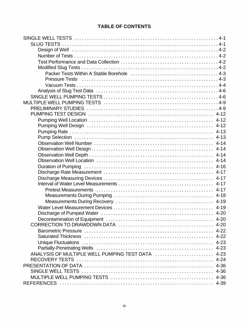
1Skin effects result from locally increasing the K near the well by opening fractures (positive skin) or decreasing the K (negative skin) byfilling voids or coating borehole walls with drilling cuttings (Sevee, 1991).
4-3
Figure 4.1 Results of a slug test with addition of water. Water arrives as an initial directpulse followed by a subsequent charge that runs down the sides of the well(Source: Adapted from Black, 1978).
Modified Slug Tests
In addition to removal or displacement of water, a change in static water level can be accomplishedby pressurizing a well with air or water or by creating a vacuum. Packers are often used to seal thezone to be tested.
Packer Tests Within A Stable Borehole
Horizontal K for consolidated rock can be determined by a packer test conducted in a stableborehole (Sevee, 1991). A single packer system can be used when testing between a packer andthe bottom of the borehole (Figure 4.2A). Two packer systems can be utilized in a completedborehole at any position or interval (Figure 4.2B). A packer is inflated using water or gas. Watershould be injected for a given length of time to test the packed-off zone.
Pressure Tests
A pulse or a pressure test may be appropriate in formations where K can be assumed to be lowerthan 10-7 cm/sec. In a pulse test, an increment of pressure is applied into a packed zone. Thedecay of pressure is monitored over a period of time using pressure transducers with electronicdata loggers or strip-chart recorders. The rate of decay is related to the K and S of the formationbeing tested. This test generally is applied in rock formations characterized by low K.Compensation must be made for skin effects1 and packer adjustments during the test. Anunderstanding of the presence and orientation of fractures is necessary to select an appropriatetype curve to analyze test data (Sevee, 1991).
4-4
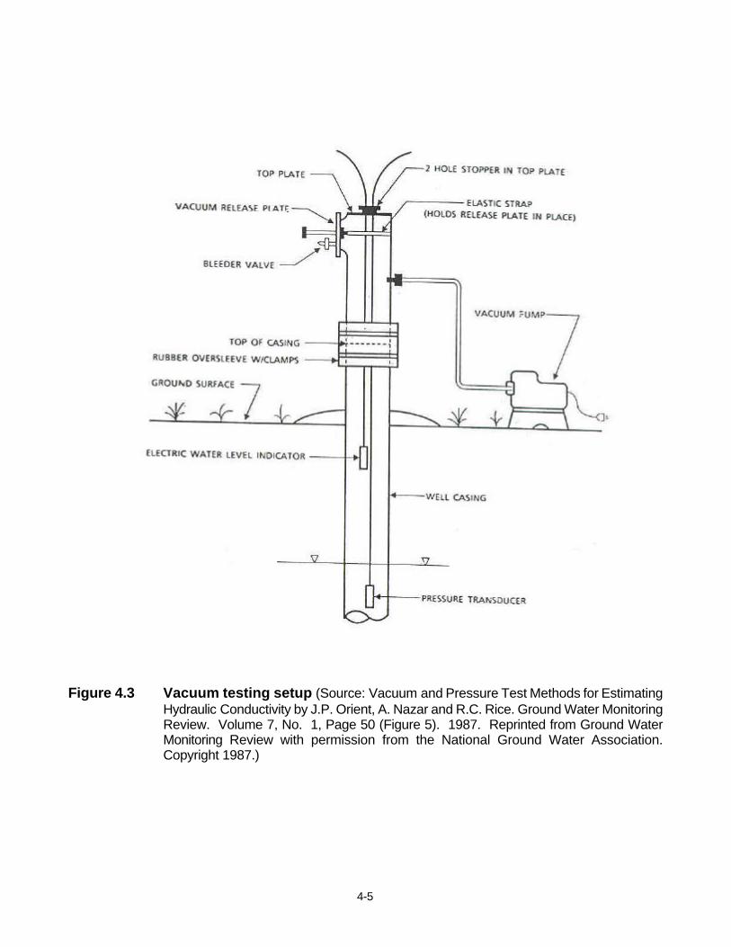
Vacuum Tests
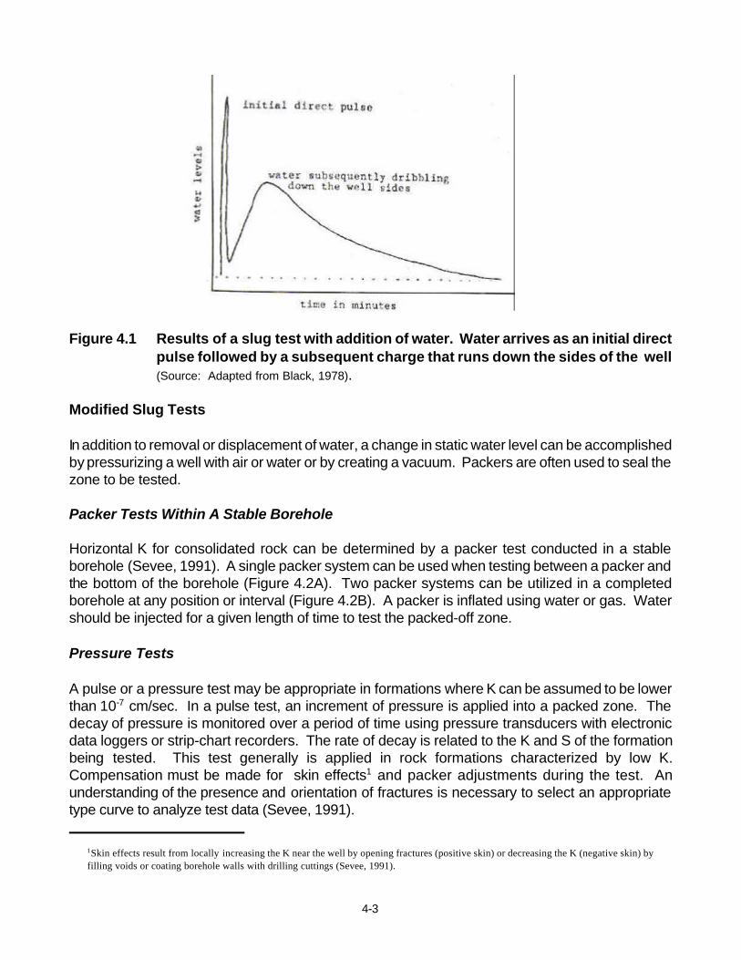
According to Orient et al. (1987), vacuum tests can be used to evaluate the K of glacial depositsand compare favorably to more conventional methods. Figure 4.3 shows typical test design. Ingeneral, water level is raised by inducing vacuum conditions. Once it reaches the desired heightand sufficient time has been allowed for the formation to return to its previous hydrostaticequilibrium, the vacuum is broken and the recovery is monitored. The data is evaluated using thesame techniques that are used to evaluate conventional slug test data.
Figure 4.2 In-Situ packer testing. A - Single packer system, test conducted during drilling. B - Doublepacker system, test conducted after borehole is complete (Source: Design and Installation of Ground WaterMonitoring Wells by D.M. Nielsen and R. Schalla, Practical Handbook of Ground Water Monitoring, edited by David M. Nielsen,
Copyright © 1991 by permission.) Lewis Publishers, an imprint of CRC Press, Boca Raton, Florida.With permission.)
Copyright requirements preclude including thefigure on Ohio EPA’s Web page. Please seeoriginal source.
4-5
Figure 4.3 Vacuum testing setup (Source: Vacuum and Pressure Test Methods for EstimatingHydraulic Conductivity by J.P. Orient, A. Nazar and R.C. Rice. Ground Water MonitoringReview. Volume 7, No. 1, Page 50 (Figure 5). 1987. Reprinted from Ground WaterMonitoring Review with permission from the National Ground Water Association.Copyright 1987.)
4-6
T '43.08Q
Sw
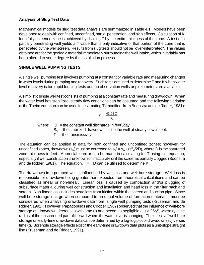
Analysis of Slug Test Data
Mathematical models for slug test data analysis are summarized in Table 4.1. Models have beendeveloped to deal with confined, unconfined, partial penetration, and skin effects. Calculation of Kfor a fully screened zone is achieved by dividing T by the entire thickness of the zone. A test of apartially penetrating well yields a T value that is only indicative of that portion of the zone that ispenetrated by the well screen. Results from slug tests should not be "over-interpreted". The valuesobtained are for the geologic material immediately surrounding the well intake, which invariably hasbeen altered to some degree by the installation process.
SINGLE WELL PUMPING TESTS
A single well pumping test involves pumping at a constant or variable rate and measuring changesin water levels during pumping and recovery. Such tests are used to determine T and K when waterlevel recovery is too rapid for slug tests and no observation wells or piezometers are available.
A simplistic single well test consists of pumping at a constant rate and measuring drawdown. Whenthe water level has stabilized, steady flow conditions can be assumed and the following variationof the Theim equation can be used for estimating T (modified from Boonstra and de Ridder, 1981):
where: Q = the constant well discharge in feet3/day.Sw = the stabilized drawdown inside the well at steady flow in feet.T = the transmissivity.
The equation can be applied to data for both confined and unconfined zones; however, forunconfined zones, drawdown (sw) must be corrected to sw' = sw - (s2
w/2D), where D is the saturatedzone thickness in feet. Appreciable error can be made in calculating for T using this equation,especially if well construction is unknown or inaccurate or if the screen is partially clogged (Boonstraand de Ridder, 1981). The equation, T = KD can be utilized to determine K.
The drawdown in a pumped well is influenced by well loss and well-bore storage. Well loss isresponsible for drawdown being greater than expected from theoretical calculations and can beclassified as linear or non-linear. Linear loss is caused by compaction and/or plugging ofsubsurface material during well construction and installation and head loss in the filter pack andscreen. Non-linear loss includes head loss from friction within the screen and suction pipe. Sincewell-bore storage is large when compared to an equal volume of formation material, it must beconsidered when analyzing drawdown data from single well pumping tests (Kruseman and deRidder, 1991). However, Papadopulos and Cooper (1967) observed that the influence of well-borestorage on drawdown decreases with time (t) and becomes negligible at t > 25rc
2, where rc is theradius of the unscreened part of the well where the water level is changing. The effects of well-borestorage on early-time drawdown data can be determined by a log-log plot of drawdown (sw) versestime (t). Borehole storage effects exist if the early-time drawdown data plots as a unit-slope straightline (Kruseman and de Ridder, 1991).
Table 4.1 Analysis methods for slug tests.
GENERAL ASSUMPTIONS 1. The aquifer has an apparently infinite areal extent.2. The zone is homogeneous and of uniform thickness over the area influenced by the test (except when noted in application column).3. Prior to the test, the water table or piezometric surface is (nearly) horizontal over the area influenced and extends infinitely in the radial direction. 4. The head in the well is changed instantaneously at time to = 0.5. The inertia of the water column in the well and the linear and non-linear well losses are negligible (i.e., well installation and development process are assumed
to have not changed the hydraulic characteristics of the formation).6. The well diameter is finite; hence storage in the well cannot be neglected. 7. Ground water density and viscosity are constant.8 No phases other than water (such as gasoline) are assumed to be present in the well or saturated portion of the aquifer.9. Ground water flow can be described by Darcy's Law.10. Water is assumed to flow horizontally.
APPLICATION
METHOD "Aquifer"Type
FlowCondition
Can account for ADDITIONALASSUMPTIONS
PROCEDURE/ANALYSIS REMARKS
PartialPenetration
Anisotropic
Cooper et al.(1967) (a,b)
Confined Transient No No - The rate at which thewater flows from the wellinto the aquifer (or viceversa) is equal to the rateat which the volume ofwater stored in the wellchanges as the head inthe well falls or rises
- Conventional**
- Type curve analysis
Difficult to match due tosimilarities of type curve.
- Also described inASTM D4104-91 (1992)
Bouwer andRice (1976)Bouwer (1989)(a,b)
Unconfinedor leaky*
Steadystate
Yes No - Aquifer isincompressible
- Buildup of the watertable is small comparedto aquifer thickness
- Conventional**
- Calculations based onmodified Theim equationand geometric parameters
- Can be used toestimate the K of leakyaquifers that receivewater from the upper-semi confining layerthrough recharge orcompression
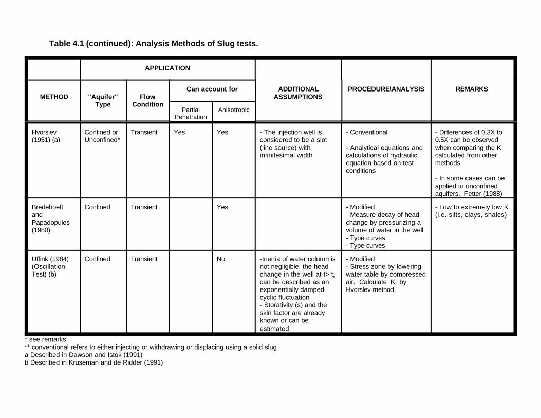
Table 4.1 (continued): Analysis Methods of Slug tests.
APPLICATION
METHOD "Aquifer"Type
FlowCondition
Can account for ADDITIONALASSUMPTIONS
PROCEDURE/ANALYSIS REMARKS
PartialPenetration
Anisotropic
Hvorslev(1951) (a)
Confined orUnconfined*
Transient Yes Yes - The injection well isconsidered to be a slot(line source) withinfinitesimal width
- Conventional
- Analytical equations andcalculations of hydraulicequation based on testconditions
- Differences of 0.3X to0.5X can be observedwhen comparing the Kcalculated from othermethods
- In some cases can beapplied to unconfinedaquifers, Fetter (1988)
BredehoeftandPapadopulos(1980)
Confined Transient Yes - Modified- Measure decay of headchange by pressurizing avolume of water in the well- Type curves- Type curves
- Low to extremely low K(i.e. silts, clays, shales)
Uffink (1984)(OscillationTest) (b)
Confined Transient No -Inertia of water column isnot negligible, the headchange in the well at t> tocan be described as anexponentially damped cyclic fluctuation- Storativity (s) and theskin factor are alreadyknown or can beestimated
- Modified- Stress zone by loweringwater table by compressedair. Calculate K byHvorslev method.
* see remarks** conventional refers to either injecting or withdrawing or displacing using a solid sluga Described in Dawson and Istok (1991)b Described in Kruseman and de Ridder (1991)
4-9
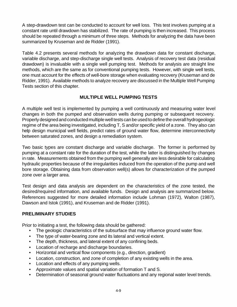
A step-drawdown test can be conducted to account for well loss. This test involves pumping at aconstant rate until drawdown has stabilized. The rate of pumping is then increased. This processshould be repeated through a minimum of three steps. Methods for analyzing the data have beensummarized by Kruseman and de Ridder (1991).
Table 4.2 presents several methods for analyzing the drawdown data for constant discharge,variable discharge, and step-discharge single well tests. Analysis of recovery test data (residualdrawdown) is invaluable with a single well pumping test. Methods for analysis are straight linemethods, which are the same as for conventional pumping tests. However, with single well tests,one must account for the effects of well-bore storage when evaluating recovery (Kruseman and deRidder, 1991). Available methods to analyze recovery are discussed in the Multiple Well PumpingTests section of this chapter.
MULTIPLE WELL PUMPING TESTS
A multiple well test is implemented by pumping a well continuously and measuring water levelchanges in both the pumped and observation wells during pumping or subsequent recovery.Properly designed and conducted multiple well tests can be used to define the overall hydrogeologicregime of the area being investigated, including T, S and/or specific yield of a zone. They also canhelp design municipal well fields, predict rates of ground water flow, determine interconnectivitybetween saturated zones, and design a remediation system.
Two basic types are constant discharge and variable discharge. The former is performed bypumping at a constant rate for the duration of the test, while the latter is distinguished by changesin rate. Measurements obtained from the pumping well generally are less desirable for calculatinghydraulic properties because of the irregularities induced from the operation of the pump and wellbore storage. Obtaining data from observation well(s) allows for characterization of the pumpedzone over a larger area.
Test design and data analysis are dependent on the characteristics of the zone tested, thedesired/required information, and available funds. Design and analysis are summarized below.References suggested for more detailed information include Lohman (1972), Walton (1987),Dawson and Istok (1991), and Kruseman and de Ridder (1991).
PRELIMINARY STUDIES
Prior to initiating a test, the following data should be gathered:• The geologic characteristics of the subsurface that may influence ground water flow.• The type of water-bearing zone and its lateral and vertical extent.• The depth, thickness, and lateral extent of any confining beds.• Location of recharge and discharge boundaries.• Horizontal and vertical flow components (e.g., direction, gradient) • Location, construction, and zone of completion of any existing wells in the area. • Location and effects of any pumping wells. • Approximate values and spatial variation of formation T and S.• Determination of seasonal ground water fluctuations and any regional water level trends.
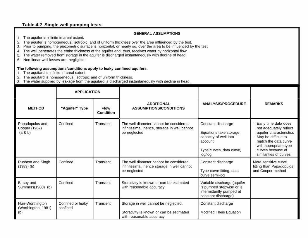
Table 4.2 Single well pumping tests.
GENERAL ASSUMPTIONS1. The aquifer is infinite in areal extent.2. The aquifer is homogeneous, isotropic, and of uniform thickness over the area influenced by the test.3. Prior to pumping, the piezometric surface is horizontal, or nearly so, over the area to be influenced by the test.4. The well penetrates the entire thickness of the aquifer and, thus, receives water by horizontal flow.5. The water removed from storage in the aquifer is discharged instantaneously with decline of head.6. Non-linear well losses are negligible.
The following assumptions/conditions apply to leaky confined aquifers.1. The aquitard is infinite in areal extent.2. The aquitard is homogeneous, isotropic and of uniform thickness. 3. The water supplied by leakage from the aquitard is discharged instantaneously with decline in head.
APPLICATION
METHOD "Aquifer" Type FlowCondition
ADDITIONALASSUMPTIONS/CONDITIONS
ANALYSIS/PROCEDURE REMARKS
Papadopulos andCooper (1967) (a & b)
Confined Transient The well diameter cannot be consideredinfinitesimal, hence, storage in well cannotbe neglected
Constant discharge
Equations take storage capacity of well intoaccount
Type curves, data curve,log/log
- Early time data doesnot adequately reflectaquifer characteristics
- May be difficult tomatch the data curvewith appropriate typecurves because ofsimilarities of curves
Rushton and Singh(1983) (b)
Confined Transient The well diameter cannot be consideredinfinitesimal, hence storage in well cannotbe neglected
Constant discharge
Type curve fitting, datacurve semi-log
More sensitive curvefitting than Papadopulosand Cooper method
Birsoy andSummers(1980) (b)
Confined Transient Storativity is known or can be estimatedwith reasonable accuracy
Variable discharge (aquiferis pumped stepwise or isintermittently pumped atconstant discharge)
Hurr-Worthington(Worthington, 1981)(b)
Confined or leakyconfined
Transient Storage in well cannot be neglected.
Storativity is known or can be estimatedwith reasonable accuracy
Constant discharge
Modified Theis Equation

Table 4.2 (Continued): Single well pumping tests.
APPLICATION
METHOD "Aquifer" Type FlowCondition
ADDITIONALASSUMPTIONS/CONDITIONS
ANALYSIS/PROCEDURE REMARKS
t < 25r 2c
KD
t < cS20
Jacob's Straight LineMethod (b)
Confined or leakyconfined
Transient For confined,
if net effect ofwell borestorage can be neglected.
For leaky, 25r 2c
KD< t < cS
20
as long as the influence ofleakage is negligible.
Constant discharge
T determined by drawdowndifferences
Sensitive to minorvariations in dischargerate
May be able to accountfor partial penetration iflate-time data is used
Hantush (1959b) (b) Leakyconfined/artesian
Transient Flow through aquitard is vertical
Aquitard is incompressible (i.e. changes inaquitard storage are negligible)
At the beginning of the test (t=0), the waterlevel in the well is lowered instantly, at t>0,the drawdown in the well is constant andits discharge is variable
Variable discharge
Type curve matching
Jacob and Lohman(1952)(b)
Confined/artesian Transient At the beginning of the test (t=0), waterlevels screened in the artesian aquifer arelowered instantaneously.
At t>0, the drawdown is constant anddischarge is variable
Uw <0.01
Variable discharge(drawdown is constant)
If value of the effectiveradius is not known thenstorativity cannot bedetermined
a Described in Dawson and Istok (1991), b Described in Kruseman and deRidder (1991)t = time since start of pumping, KD =transmissivity of the aquifer, rc = radius of the unscreend part of the well where water level is changing, c = hydraulic resistance of theaquitard, S = storativity, Uw = equation function
4-12
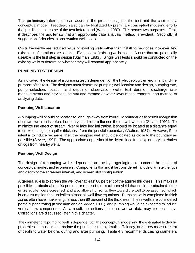
This preliminary information can assist in the proper design of the test and the choice of aconceptual model. Test design also can be facilitated by preminary conceptual modeling effortsthat predict the outcome of the test beforehand (Walton, 1987). This serves two purposes. First,it describes the aquifer so that an appropriate data analysis method is evident. Secondly, itsuggests deficiencies in observation well locations.
Costs frequently are reduced by using existing wells rather than installing new ones; however, fewexisting configurations are suitable. Evaluation of existing wells to identify ones that are potentiallyuseable is the first step in design (Stallman, 1983). Single well tests should be conducted on theexisting wells to determine whether they will respond appropriately.
PUMPING TEST DESIGN
As indicated, the design of a pumping test is dependent on the hydrogeologic environment and thepurpose of the test. The designer must determine pumping well location and design, pumping rate,pump selection, location and depth of observation wells, test duration, discharge ratemeasurements and devices, interval and method of water level measurements, and method ofanalyzing data.
Pumping Well Location
A pumping well should be located far enough away from hydraulic boundaries to permit recognitionof drawdown trends before boundary conditions influence the drawdown data (Sevee, 1991). Tominimize the effect of stream, river or lake bed infiltration, it should be located at a distance equalto or exceeding the aquifer thickness from the possible boundary (Walton, 1987). However, if theintent is to induce recharge, then the pumping well should be located as close to the boundary aspossible (Sevee, 1991). The appropriate depth should be determined from exploratory boreholesor logs from nearby wells.
Pumping Well Design
The design of a pumping well is dependent on the hydrogeologic environment, the choice ofconceptual model, and economics. Components that must be considered include diameter, lengthand depth of the screened interval, and screen slot configuration.
A general rule is to screen the well over at least 80 percent of the aquifer thickness. This makes itpossible to obtain about 90 percent or more of the maximum yield that could be obtained if theentire aquifer were screened, and also allows horizontal flow toward the well to be assumed, whichis an assumption that underlies almost all well-flow equations. Pumping wells completed in thickzones often have intake lengths less than 80 percent of the thickness. These wells are consideredpartially-penetrating (Kruseman and deRidder, 1991), and pumping would be expected to inducevertical flow components. As a result, corrections to the drawdown data may be necessary.Corrections are discussed later in this chapter.
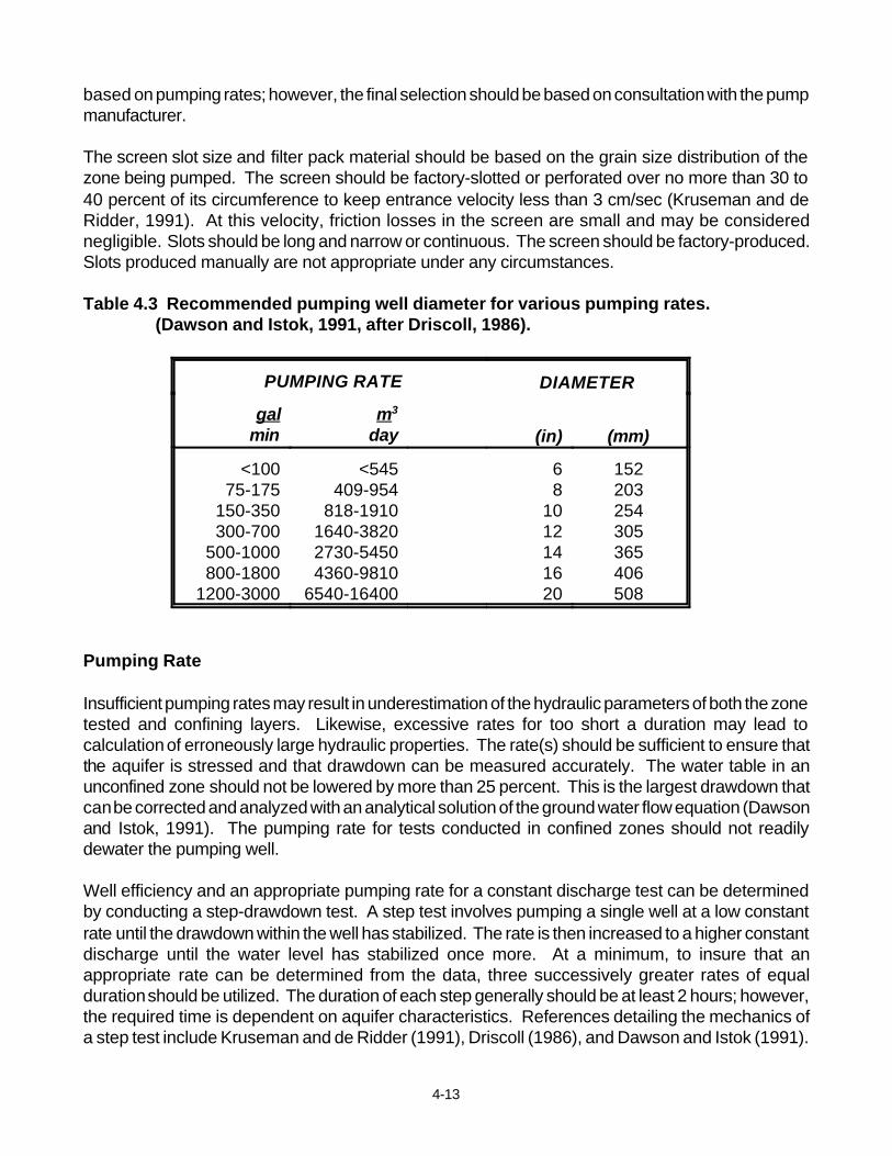
The diameter of a pumping well is dependent on the conceptual model and the estimated hydraulicproperties. It must accommodate the pump, assure hydraulic efficiency, and allow measurementof depth to water before, during and after pumping. Table 4.3 recommends casing diameters
4-13
based on pumping rates; however, the final selection should be based on consultation with the pumpmanufacturer.
The screen slot size and filter pack material should be based on the grain size distribution of thezone being pumped. The screen should be factory-slotted or perforated over no more than 30 to40 percent of its circumference to keep entrance velocity less than 3 cm/sec (Kruseman and deRidder, 1991). At this velocity, friction losses in the screen are small and may be considerednegligible. Slots should be long and narrow or continuous. The screen should be factory-produced.Slots produced manually are not appropriate under any circumstances.
Table 4.3 Recommended pumping well diameter for various pumping rates.(Dawson and Istok, 1991, after Driscoll, 1986).
PUMPING RATE DIAMETER
galmin
m3
day (in) (mm)
<10075-175
150-350300-700
500-1000800-1800
1200-3000
<545409-954
818-19101640-38202730-54504360-9810
6540-16400
68
1012141620
152203254305365406508
Pumping Rate
Insufficient pumping rates may result in underestimation of the hydraulic parameters of both the zonetested and confining layers. Likewise, excessive rates for too short a duration may lead tocalculation of erroneously large hydraulic properties. The rate(s) should be sufficient to ensure thatthe aquifer is stressed and that drawdown can be measured accurately. The water table in anunconfined zone should not be lowered by more than 25 percent. This is the largest drawdown thatcan be corrected and analyzed with an analytical solution of the ground water flow equation (Dawsonand Istok, 1991). The pumping rate for tests conducted in confined zones should not readilydewater the pumping well.
Well efficiency and an appropriate pumping rate for a constant discharge test can be determinedby conducting a step-drawdown test. A step test involves pumping a single well at a low constantrate until the drawdown within the well has stabilized. The rate is then increased to a higher constantdischarge until the water level has stabilized once more. At a minimum, to insure that anappropriate rate can be determined from the data, three successively greater rates of equalduration should be utilized. The duration of each step generally should be at least 2 hours; however,the required time is dependent on aquifer characteristics. References detailing the mechanics ofa step test include Kruseman and de Ridder (1991), Driscoll (1986), and Dawson and Istok (1991).
4-14
Other methods that may be useful to estimate an appropriate pumping rate for a constant head testinclude: 1) using an empirical formula to predict well specific capacity, and 2) predicting drawdownusing analytical solutions. These methods are described by Dawson and Istok (1991). It should benoted that these techniques predict discharge rates that can be utilized to determine hydraulicparameters and should not be utilized to estimate an appropriate rate for capturing a contaminantplume.
Pump Selection
The pump and power supply must be capable of operating continuously at an appropriate constantdischarge rate for at least the expected duration of the test. Pumps powered by electric motorsproduce the most constant discharge (Stallman, 1983).
Observation Well Number
The appropriate number of observation wells depends on the goals of the test, hydrogeologiccomplexity, the degree of accuracy needed, and economics. Though it is always best to have asmany wells as conditions permit, at least three should be employed in the pumping zone (Krusemanand de Ridder, 1991). If two or more are available, data can be analyzed by both drawdown versustime and drawdown versus distance relationships. Using both and observing how wells respondin various locations provides greater assurance that: 1) the calculated hydraulic properties arerepresentative of the zone being pumped over a large area, and 2) any heterogeneities that mayaffect the flow of ground water and contaminants have been identified. In areas in where severalcomplex boundaries exist, additional wells may be needed to allow proper interpretation of the testdata (Sevee, 1991).
Observation Well Design
In general, observation wells need to be constructed with an appropriate filter pack, screen slot size,and annular seal, and must be developed properly. Practices for design and development ofobservation wells can be similar to those for monitoring wells (see Chapters 7 & 8). Theobservation wells/piezometers must be of sufficient diameter to accommodate the measuringdevice, but should not be so large that the drawdown cannot be measured.
Observation Well Depth
Fully-penetrating wells are desirable. The open portion of an observation well generally should beplaced vertically opposite the intake of the pumping well. When testing heterogeneous zones, it isrecommended that an observation well be installed in each permeable layer. Additional wellsshould be placed in the aquitards to determine leakage and interconnectivity (Kruseman and deRidder, 1991).
Observation Well Location
Observation well location is dependent on the type of aquifer, estimated transmissivity, duration ofthe test, discharge rate, length of the pumping well screen, whether the aquifer is stratified or
4-15
M.D.$$ 1.5 DKH
KV
fractured, and anticipated boundary conditions. Placing observation wells 10 to 100 meters (33 to328 feet) from the pumping well is generally adequate for determining hydraulic parameters. Forthick or stratified, confined zones, the distance should be greater (Kruseman and de Ridder, 1991).It also is recommended that additional observation wells be located outside the zone of influenceof the pumping well to monitor possible natural changes in head.
In general, observation wells completed in a confined zone can be spaced further from the pumpingwell than those completed in an unconfined aquifer. The decline in the piezometric surface ofconfined zones spreads rapidly because the release of water from storage is entirely due tocompressibility of water and the aquifer material. Water movement in unconfined zones isprincipally from draining of pores, which results in a slower expansion.
Under isotropic conditions, the distribution of the observation wells around the pumping well can bearbitrary. However, an even distribution is desirable so that drawdown measurements arerepresentative of the largest volume of aquifer possible (Dawson and Istok, 1991). If feasible, atleast three wells should be logarithmically spaced to provide at least one logarithmic cycle ofdistance-drawdown data (Walton, 1987). If anisotropic conditions exist or are suspected, then asingle row of observation wells is not sufficient to estimate the directional dependence oftransmissivity. A minimum of 3 observation wells, none of which are on the same radial arc, isrequired to separate the anisotropic behavior.
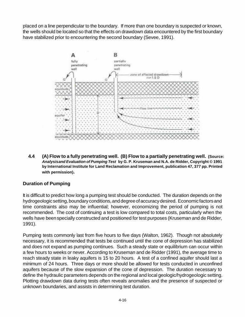
The length of the pumping well screen can have a strong influence on the distance of the observationwells from the pumping well. Partially-penetrating pumping wells will induce vertical flow, which ismost noticeable near the well (Figure 4.4). As a result, water level measurements taken from thesewells need to be corrected; however, the effects of vertical flow become more negligible atincreasing distances from the pumping well. For partially-penetrating pumping wells, correctionsto the drawdown data may not be necessary if the following relation holds true (Sevee, 1991; andDawson and Istok, 1991):
M.D. = minimum distance between pumping well and observation well.D = thickness of the aquifer.KH = horizontal K.KV = vertical K.
Drawdown measured in observation wells located less than the minimim distance should becorrected. Typically, horizontal K is ten times greater than vertical K. If this ratio is used, then theminimum distance becomes 1.5D/10. It should be noted that partially-penetrating wells locatedat or greater than the minimum distance may be too far away to show drawdown.
Anticipated boundary conditions (e.g., an impervious zone or a recharging river) also can affect theplacement of observation wells. Wells can be placed to either minimize the effect of the boundaryor more precisely locate the discontinuity (Dawson and Istok, 1991). According to Walton (1987),to minimize the effect of the boundary on distance-drawdown data, wells should be placed alonga line through the pumping well and parallel to the boundary. Observation wells also should be
4-16
placed on a line perpendicular to the boundary. If more than one boundary is suspected or known,the wells should be located so that the effects on drawdown data encountered by the first boundaryhave stabilized prior to encountering the second boundary (Sevee, 1991).
4.4 (A) Flow to a fully penetrating well. (B) Flow to a partially penetrating well. (Source:Analysis and Evaluation of Pumping Test by G. P. Kruseman and N.A. de Ridder, Copyright © 1991by International Institute for Land Reclamation and Improvement, publication 47, 377 pp. Printed
with permission).
Duration of Pumping
It is difficult to predict how long a pumping test should be conducted. The duration depends on thehydrogeologic setting, boundary conditions, and degree of accuracy desired. Economic factors andtime constraints also may be influential; however, economizing the period of pumping is notrecommended. The cost of continuing a test is low compared to total costs, particularly when thewells have been specially constructed and positioned for test purposes (Kruseman and de Ridder,1991).
Pumping tests commonly last from five hours to five days (Walton, 1962). Though not absolutelynecessary, it is recommended that tests be continued until the cone of depression has stabilizedand does not expand as pumping continues. Such a steady state or equilibrium can occur withina few hours to weeks or never. According to Kruseman and de Ridder (1991), the average time toreach steady state in leaky aquifers is 15 to 20 hours. A test of a confined aquifer should last aminimum of 24 hours. Three days or more should be allowed for tests conducted in unconfinedaquifers because of the slow expansion of the cone of depression. The duration necessary todefine the hydraulic parameters depends on the regional and local geologic/hydrogeologic setting.Plotting drawdown data during tests often reveals anomalies and the presence of suspected orunknown boundaries, and assists in determining test duration.
4-17
Discharge Rate Measurement
Variation in discharge rates produces aberrations in drawdown that are difficult to treat in dataanalysis. Engines, even those equipped with automatic speed controls, can produce variations upto 20 to 25 percent over the course of a day. The rate should never vary by more than five percent(Osborn, 1993). In order to obtain reliable data, discharge should be monitored and adjustmentsmade as needed.
The frequency of measurements is dependent on the pump, engine power characteristics, the well,and the zone tested. Discharge from electric pumps should be measured and adjusted (ifnecessary) at 5, 10, 20, 30, 60 minutes, and hourly thereafter. Other types of pumps may requiremore frequent attention; however, no "rule of thumb" can be set because of the wide variation inequipment response (Stallman, 1983).
Discharge Measuring Devices
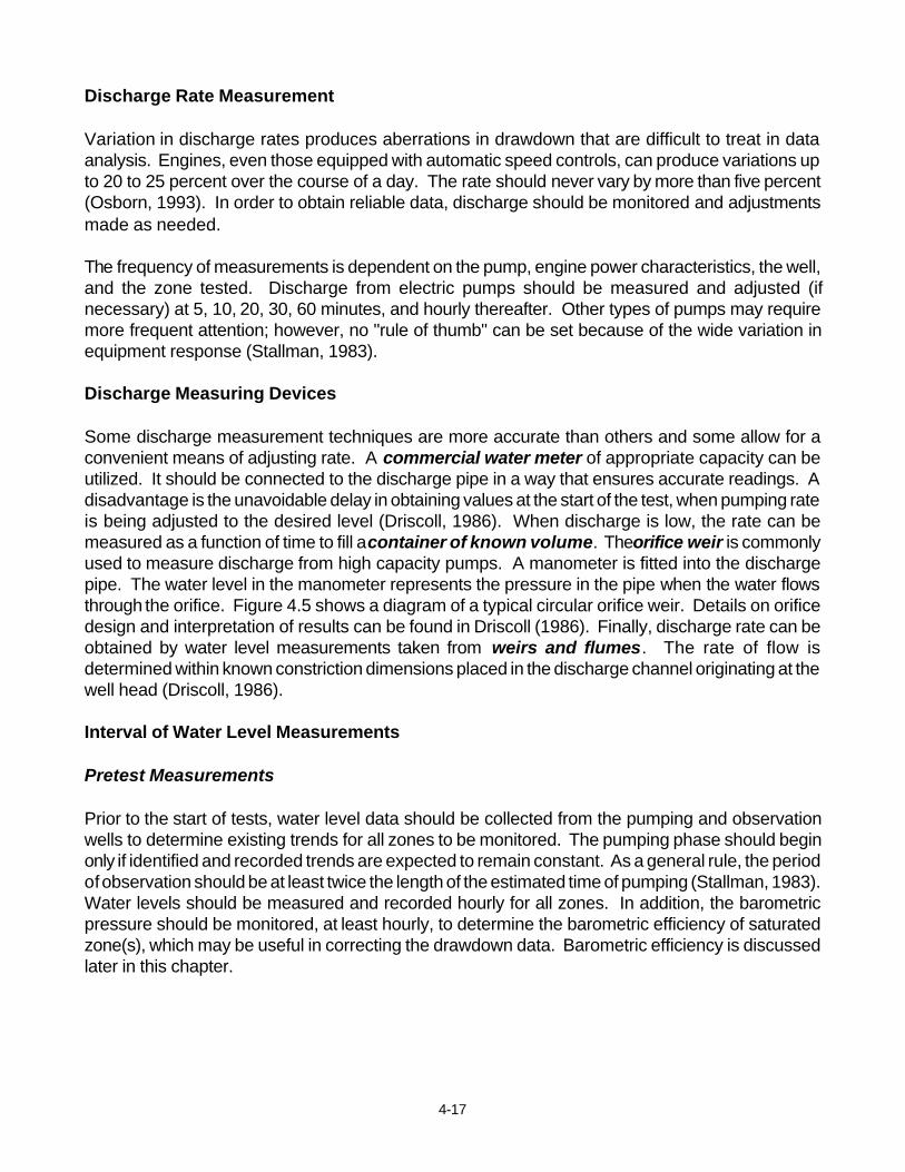
Some discharge measurement techniques are more accurate than others and some allow for aconvenient means of adjusting rate. A commercial water meter of appropriate capacity can beutilized. It should be connected to the discharge pipe in a way that ensures accurate readings. Adisadvantage is the unavoidable delay in obtaining values at the start of the test, when pumping rateis being adjusted to the desired level (Driscoll, 1986). When discharge is low, the rate can bemeasured as a function of time to fill a container of known volume. The orifice weir is commonlyused to measure discharge from high capacity pumps. A manometer is fitted into the dischargepipe. The water level in the manometer represents the pressure in the pipe when the water flowsthrough the orifice. Figure 4.5 shows a diagram of a typical circular orifice weir. Details on orificedesign and interpretation of results can be found in Driscoll (1986). Finally, discharge rate can beobtained by water level measurements taken from weirs and flumes. The rate of flow isdetermined within known constriction dimensions placed in the discharge channel originating at thewell head (Driscoll, 1986).
Interval of Water Level Measurements
Pretest Measurements
Prior to the start of tests, water level data should be collected from the pumping and observationwells to determine existing trends for all zones to be monitored. The pumping phase should beginonly if identified and recorded trends are expected to remain constant. As a general rule, the periodof observation should be at least twice the length of the estimated time of pumping (Stallman, 1983).Water levels should be measured and recorded hourly for all zones. In addition, the barometricpressure should be monitored, at least hourly, to determine the barometric efficiency of saturatedzone(s), which may be useful in correcting the drawdown data. Barometric efficiency is discussedlater in this chapter.
4-18
Figure 4.5 Construction diagram of a circular orifice weir commonly used for measuringrates of a high capacity pump. (Source: Ground Water and Wells by E.G. Driscoll.
Copyright , © 1986; Johnson screens. Printed with permission).
Measurements During Pumping
The appropriate time interval for water level measurements varies from frequent at the beginningof a test, when water-levels are changing rapidly, to long at the end of the test, when change is slow.Typical intervals for the pumping well and observation wells located close to the pumping well aregiven in Tables 4.4 and 4.5, respectively. Though specified intervals need not be followed rigidly,each logarithmic cycle of time should contain at least 10 data points spread through the cycle(Stallman, 1983). Frequent readings are essential during the first hour since the rate of change isfaster. For wells further away and those located in zones above or below the pumping zone, thefrequent measurements recommended by Table 4.5 for the first few minutes of the pumping testsare less important (Kruseman and de Ridder, 1991).

4-19
Table 4.4 Range of interval between water-level measurements in the pumping well(Kruseman and de Ridder, 1991).
TIME SINCE START OF PUMPING TIME INTERVAL
0 to 5 minutes 0.5 minutes2 to 60 minutes 5 minutes60 to 120 minutes 20 minutes 120 to shutdown of the pump 60 minutes
Table 4.5 Range of intervals between water-level measurements in observation wells(Kruseman and de Ridder, 1991).
TIME SINCE START OF PUMPING TIME INTERVAL
0 to 2 minutes2 to 5 minutes5 to 15 minutes50 to 100 minutes100 minutes to 5 hours5 hours to 48 hours48 hours to 6 days6 days to shutdown of the pump
approx. 10 seconds30 seconds1 minute5 minutes30 minutes60 minutes3 times a day1 time a day
According to Stallman (1983), it is not necessary to measure water levels in all wells simultaneously,but it is highly desirable to achieve nearly uniform separation of plotted drawdowns on a logarithmicscale. All watches used should be synchronized before the test is started, and provisions made tonotify all participants at the instant the test is initiated.
Measurements During Recovery
After pumping is completed, water level recovery should be monitored with the same frequencyused during pumping.
Water Level Measurement Devices
The most accurate recording of water level changes is made with fully automatic microcomputer-controlled systems that use pressure or acoustic transducers for continuous measurements. Waterlevels can also be determined by hand, but the instant of each reading must be recorded with achronometer. Measurements can be performed with floating steel tape equipped with a standardpointer, electronic sounder, or wet-tape method. For observation wells close to the pumped well,automatic recorders programmed for frequent measurements are most convenient because waterlevel change is rapid during the first hour of the test. For detailed descriptions of automaticrecorders, mechanical and electric sounders, and other tools, see Driscoll (1986), Dalton et al.(1991), and ASTM D4750-87 (1992). Chapter 10 of this document contains a summary of manualdevices.
4-20
The measurement procedure should be standardized and calibrated prior to the start of the test.Transducers should be calibrated by a direct method, and the calibration should be checked at theconclusion of the recovery test.
Discharge of Pumped Water
Water extracted during a pumping test must be discharged properly and in accordance with anyapplicable laws and regulations. At sites with contaminated ground water, the discharge may needto be containerized and sampled to assess the presence of contaminants and, if necessary, treatedand/or disposed at an appropriate permitted facility.
It is not the intent of this document to define Agency policy on disposal of pumped water. In general,the water should be evaluated to determine if it is characteristically a waste. If the ground water hasbeen contaminated by a listed hazardous waste, the ground water is considered to "contain" thatwaste, and must therefore be managed as such. Disposal must be at a permitted hazardous wastefacility. Treatment must be in a wastewater treatment system that is appropriate for the waste andmeets the definitions contained in OAC rule 3745-50-10.
If containerization is not necessary, then pumped water must be discharged in a manner thatprevents recharge into any zone being monitored during the test. At a minimum, the water shouldbe discharged 100 to 200 meters from the pumped well. This is particularly important when testingunconfined zones. At no time should the discharge water be injected back into the subsurface. Apermit for discharge via stream or storm sewer may be required (contact the Division of SurfaceWater, Ohio EPA).
Decontamination of Equipment
Decontamination of equipment is important throughout an in-situ test. Contact of contaminatedequipment with ground water (or a well) may cause a measuring point to be unsuitable for waterquality investigations. Details on appropriate methods can be found in Chapter 10.
CORRECTION TO DRAWDOWN DATA
Prior to using the drawdown data collected from a pumping test, it may be necessary to correct foreither external sources or effects induced by the test. Barometric pressure changes, tidal or riverfluctuations, natural recharge and discharge, and unique situations (e.g., a heavy rainfall) may allexert an influence. In confined and leaky aquifers, changes in hydraulic head may be due toinfluences of tidal or river-level fluctuations, surface loading, or changes in atmospheric pressure.
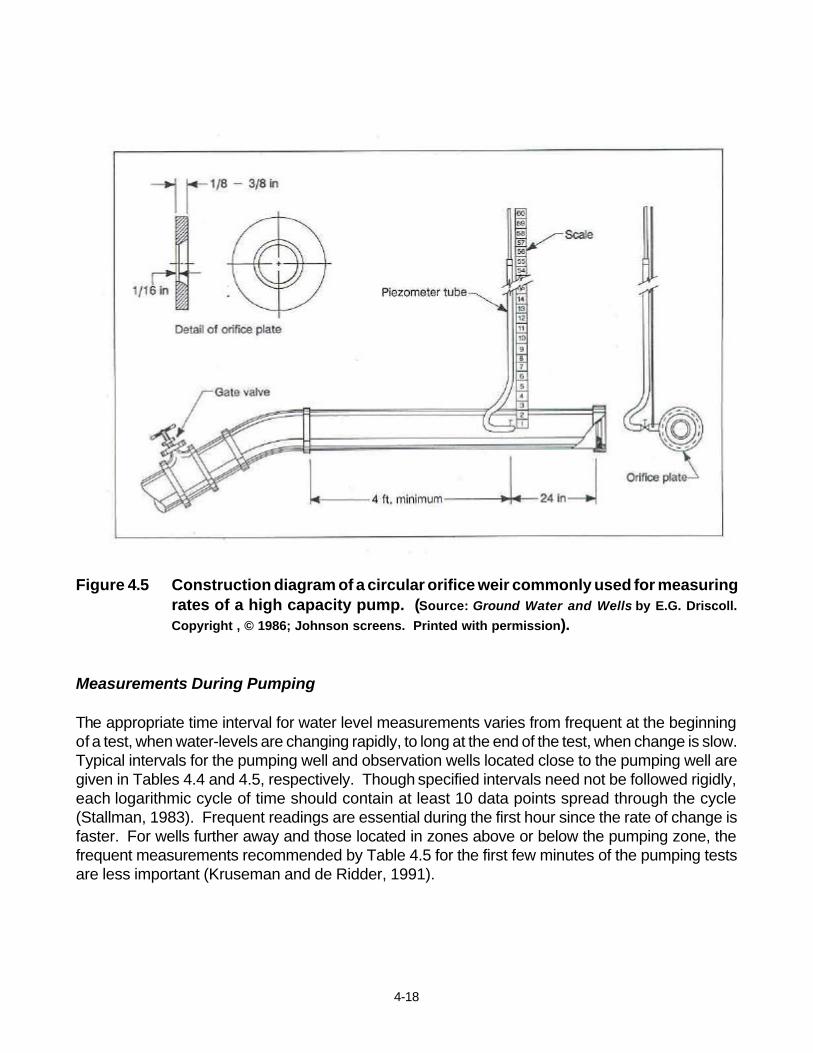
Diurnal fluctuations in water levels can occur in unconfined aquifers due to the differences betweennight and day evapotranspiration. Corrections to measurements may be needed for unconfinedaquifer data due to a decrease in saturated thickness caused by the pumping test. Also,corrections may be necessary if the pumping well only partially penetrates the zone tested. Byidentifying pre-test water level trends in zone(s) of interest, long and short-term variations can beeliminated from the data if their impacts are significant during the pumping phase (Figure 4.6).
4-21
In order to determine if corrections are necessary, measurements should be taken during the testin observation wells unaffected by the pumping. Hydrographs of the pumping and observation wellscovering a sufficient period of pre-test and post-recovery periods can help determine if the dataneeds to be corrected and also to correct the drawdown data. If the same constant water level isobserved during the pre-testing and post-recovery periods, it can safely be assumed that noexternal events exerted an influence (Kruseman and de Ridder, 1991).
Figure 4.6 Hydrograph for hypothetical observation well showing definition of drawdown(adapted from Stallman, 1983).
4-22
BE 'Mh
Mka / ãw
x 100%
Barometric Pressure
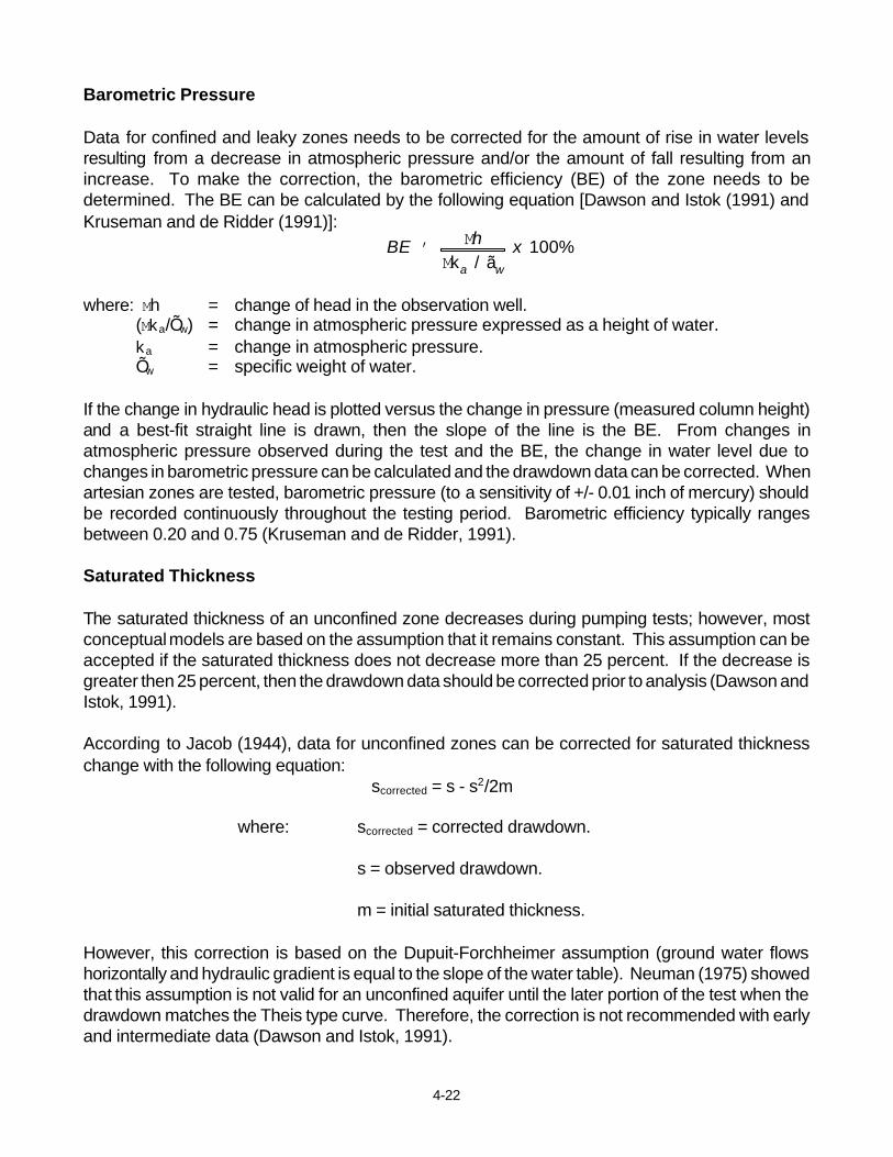
Data for confined and leaky zones needs to be corrected for the amount of rise in water levelsresulting from a decrease in atmospheric pressure and/or the amount of fall resulting from anincrease. To make the correction, the barometric efficiency (BE) of the zone needs to bedetermined. The BE can be calculated by the following equation [Dawson and Istok (1991) andKruseman and de Ridder (1991)]:
where: Mh = change of head in the observation well.(Mka/Õw) = change in atmospheric pressure expressed as a height of water.ka = change in atmospheric pressure.Õw = specific weight of water.
If the change in hydraulic head is plotted versus the change in pressure (measured column height)and a best-fit straight line is drawn, then the slope of the line is the BE. From changes inatmospheric pressure observed during the test and the BE, the change in water level due tochanges in barometric pressure can be calculated and the drawdown data can be corrected. Whenartesian zones are tested, barometric pressure (to a sensitivity of +/- 0.01 inch of mercury) shouldbe recorded continuously throughout the testing period. Barometric efficiency typically rangesbetween 0.20 and 0.75 (Kruseman and de Ridder, 1991).
Saturated Thickness
The saturated thickness of an unconfined zone decreases during pumping tests; however, mostconceptual models are based on the assumption that it remains constant. This assumption can beaccepted if the saturated thickness does not decrease more than 25 percent. If the decrease isgreater then 25 percent, then the drawdown data should be corrected prior to analysis (Dawson andIstok, 1991).
According to Jacob (1944), data for unconfined zones can be corrected for saturated thicknesschange with the following equation:
scorrected = s - s2/2m
where: scorrected = corrected drawdown.
s = observed drawdown.
m = initial saturated thickness.
However, this correction is based on the Dupuit-Forchheimer assumption (ground water flowshorizontally and hydraulic gradient is equal to the slope of the water table). Neuman (1975) showedthat this assumption is not valid for an unconfined aquifer until the later portion of the test when thedrawdown matches the Theis type curve. Therefore, the correction is not recommended with earlyand intermediate data (Dawson and Istok, 1991).
4-23
Unique Fluctuations
Data cannot be corrected for unique events such as a heavy rain or sudden fall or rise of a nearbyriver that is hydraulically connected to the zone tested. However, in favorable circumstances, someallowances can be made for the resulting fluctuations by extrapolating data from a controlledpiezometer outside the zone of influence. In most cases, the data collected is rendered worthlessand the test has to be repeated when the situation returns to normal (Kruseman and de Ridder,1991). It is also important to understand the effects of nearby industrial or municipal pumping wellsprior to conducting a pumping test.
Partially-Penetrating Wells
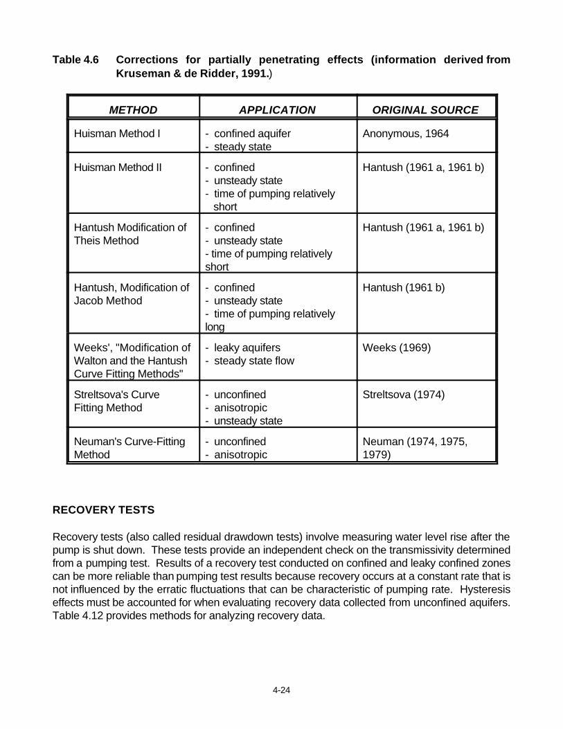
In some cases, a saturated zone is so thick that it is not justifiable to install a fully-penetrating well,and the aquifer must be pumped by a partially-penetrating well. Partial-penetration causes verticalflow in the vicinity of the well, which results in additional head loss. As indicated earlier, this effectdecreases with increasing distance from the pumping well and no correction is necessary if theobservation well is at a distance greater than 1.5 D/KH/KV. Various methods have been developedto correct data for the effects of partially-penetrating wells. These were discussed in detail byKruseman and de Ridder (1991). Table 4.6 lists the methods and their general applications.
ANALYSIS OF MULTIPLE WELL PUMPING TEST DATA
Many conceptual models exist for interpreting multiple well pumping test data. The hydraulicproperties computed by a particular method can only be considered correct if the assumptionsincluded in the conceptual model on which the method is based are valid for the particular systembeing tested. Because the computed values depend on the choice of conceptual model used toanalyze the data, the selection of an appropriate model is the single most important step in analysis(Dawson and Istok, 1991).
IIt is beyond the scope of this document to detail or discuss all conceptual models. Tables 4.7through 4.11 can be used for a preliminary selection. In addition, the ASTM Method D4043-91(1992) provides a decision tree for the selection of an aquifer test method and ASTM MethodsD4106-91 (1992) and D4105-91 (1992) offer information on determining hydraulic parameters.Additional references are provided in the tables that should serve as a guide for choice and use ofconceptual models. It should be noted that additional models may exist that are not listed here. Anymodel utilized must be shown to be appropriate for site conditions.
Data collected during a pumping test are subject to a variety of circumstances that may berecognized in the field or may not be apparent until data analysis has begun. In either case, allinformation (including field observations) must be examined during data correlation and analysis.
4-24
Table 4.6 Corrections for partially penetrating effects (information derived fromKruseman & de Ridder, 1991.)
METHOD APPLICATION ORIGINAL SOURCE
Huisman Method I - confined aquifer- steady state
Anonymous, 1964
Huisman Method II - confined- unsteady state- time of pumping relatively short
Hantush (1961 a, 1961 b)
Hantush Modification ofTheis Method
- confined- unsteady state- time of pumping relatively short
Hantush (1961 a, 1961 b)
Hantush, Modification ofJacob Method
- confined- unsteady state- time of pumping relatively long
Hantush (1961 b)
Weeks', "Modification ofWalton and the HantushCurve Fitting Methods"
- leaky aquifers- steady state flow
Weeks (1969)
Streltsova's CurveFitting Method
- unconfined- anisotropic- unsteady state
Streltsova (1974)
Neuman's Curve-FittingMethod
- unconfined- anisotropic
Neuman (1974, 1975,1979)
RECOVERY TESTS
Recovery tests (also called residual drawdown tests) involve measuring water level rise after thepump is shut down. These tests provide an independent check on the transmissivity determinedfrom a pumping test. Results of a recovery test conducted on confined and leaky confined zonescan be more reliable than pumping test results because recovery occurs at a constant rate that isnot influenced by the erratic fluctuations that can be characteristic of pumping rate. Hysteresiseffects must be accounted for when evaluating recovery data collected from unconfined aquifers.Table 4.12 provides methods for analyzing recovery data.
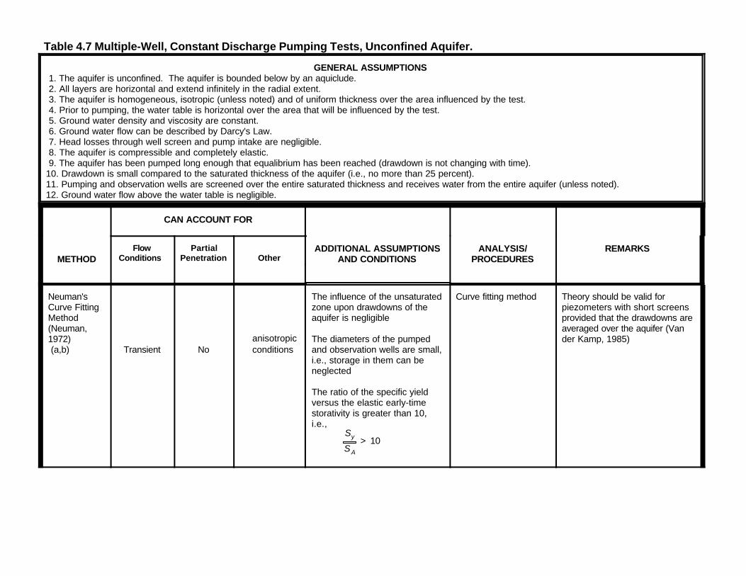
Table 4.7 Multiple-Well, Constant Discharge Pumping Tests, Unconfined Aquifer.
GENERAL ASSUMPTIONS 1. The aquifer is unconfined. The aquifer is bounded below by an aquiclude. 2. All layers are horizontal and extend infinitely in the radial extent. 3. The aquifer is homogeneous, isotropic (unless noted) and of uniform thickness over the area influenced by the test. 4. Prior to pumping, the water table is horizontal over the area that will be influenced by the test. 5. Ground water density and viscosity are constant. 6. Ground water flow can be described by Darcy's Law. 7. Head losses through well screen and pump intake are negligible. 8. The aquifer is compressible and completely elastic. 9. The aquifer has been pumped long enough that equalibrium has been reached (drawdown is not changing with time).10. Drawdown is small compared to the saturated thickness of the aquifer (i.e., no more than 25 percent).11. Pumping and observation wells are screened over the entire saturated thickness and receives water from the entire aquifer (unless noted).12. Ground water flow above the water table is negligible.
CAN ACCOUNT FOR
METHODFlow
Conditions Partial
Penetration OtherADDITIONAL ASSUMPTIONS
AND CONDITIONSANALYSIS/
PROCEDURESREMARKS
Neuman'sCurve FittingMethod(Neuman,1972) (a,b)
Transient Noanisotropicconditions
The influence of the unsaturatedzone upon drawdowns of theaquifer is negligible
The diameters of the pumpedand observation wells are small,i.e., storage in them can beneglected
The ratio of the specific yieldversus the elastic early-timestorativity is greater than 10,i.e.,
Sy
SA
> 10
Curve fitting method Theory should be valid forpiezometers with short screensprovided that the drawdowns areaveraged over the aquifer (Vander Kamp, 1985)
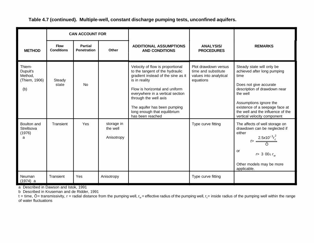
Table 4.7 (continued). Multiple-well, constant discharge pumping tests, unconfined aquifers.
CAN ACCOUNT FOR
METHODFlow
Conditions Partial
Penetration OtherADDITIONAL ASSUMPTIONS
AND CONDITIONSANALYSIS/
PROCEDURESREMARKS
t>2.5x10& 3r 2
c
Ô
r> 3 00& rw
Thiem-Dupuit'sMethod,(Thiem, 1906)
(b)
Steadystate No
Velocity of flow is proportionalto the tangent of the hydraulicgradient instead of the sine as itis in reality
Flow is horizontal and uniformeverywhere in a vertical sectionthrough the well axis
The aquifer has been pumpinglong enough that equilibriumhas been reached
Plot drawdown versustime and substitutevalues into analyticalequations
Steady state will only beachieved after long pumpingtime
Does not give accuratedescription of drawdown nearthe well
Assumptions ignore theexistence of a seepage face atthe well and the influence of thevertical velocity component
Boulton andStreltsova(1976) a
Transient Yes storage inthe well
Anisotropy
Type curve fitting The affects of well storage on drawdown can be neglected ifeither
or
Other models may be moreapplicable.
Neuman(1974) a
Transient Yes Anisotropy Type curve fitting
a Described in Dawson and Istok, 1991b Described in Kruseman and de Ridder, 1991t = time, Ô = transmissivity, r = radial distance from the pumping well, rw = effective radius of the pumping well, rc= inside radius of the pumping well within the rangeof water fluctuations

Table 4.8 Multiple-well, constant-discharge pumping tests, confined aquifers.
GENERAL ASSUMPTIONS1. The aquifer is confined. The aquifer is bounded above and below by aquicludes.2. The aquifer is homogeneous, isotropic (unless noted in special conditions) and of uniform thickness over the area influenced by the test.3. All layers are horizontal and extend infinitely in the radial extent.4. Prior to pumping, the piezometric surface is horizontal and extends infinitely in the radial direction.5. Ground water density and viscosity are constant.6. Ground water can be described by Darcy's Law.7. Head losses through well screen and pump intake are negligible.8. Ground water flow is horizontal and is directed radially to the well.9. Pumping well and observation wells are screened over the entire thickness of the aquifer.
Additional assumptions for unsteady state flow.10. The water removed from storage is discharged instantaneously with decline of head.11. The diameter of the well is small, i.e., the storage in the well can be neglected.
APPLICATION
METHOD FlowCondition
CAN ACCOUNT FOR
ADDITIONAL ASSUMPTIONSAND CONDITIONS
ANALYSIS/PROCEDURES
REMARKS
PartialPenetration
Other
Thiem (1906) (a, b) Steady
state No
The aquifer has been pumpedlong enough that equilibrium hasbeen reached (drawdown is notchanged with time)
Drawdown versus timeplotted on semi-log paperand substitution of valuesinto analytical equations.
Equation should be used withcaution and only when othermethods cannot be applied
Drawdown is influenced by welllosses, screen and pump intake
Theis (1935)
(a,b) Transient No
The aquifer is compressible andcompletely elastic
Type curve analysis Because there may be a timelag between pressure declineand release of stored water,early drawdown data may notclosely represent theoreticaldrawdown data
Hantush(1964) (b)
Transient YesAnisotropy inthe horizontalplane
No vertical flow at the top andbottom of the aquifer
Solutions involve typecurve analysis orinflection point method
Inflection point method can beused when the horizontal andvertical hydraulic conductivitiescan be reasonably estimated.
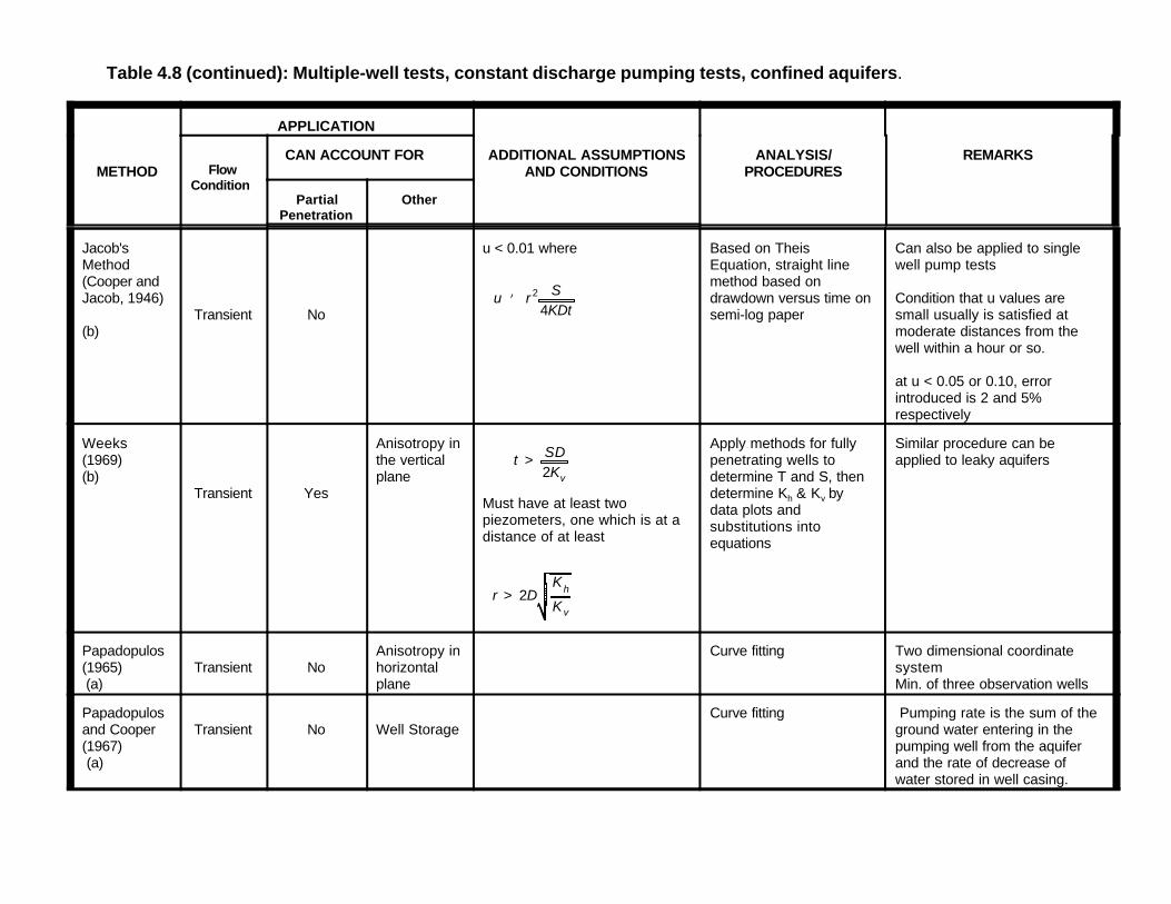
Table 4.8 (continued): Multiple-well tests, constant discharge pumping tests, confined aquifers.
APPLICATION
METHOD FlowCondition
CAN ACCOUNT FOR
ADDITIONAL ASSUMPTIONSAND CONDITIONS
ANALYSIS/PROCEDURES
REMARKS
PartialPenetration
Other
Jacob'sMethod (Cooper and Jacob, 1946)
(b)Transient No
u < 0.01 where
u ' r 2 S4KDt
Based on TheisEquation, straight linemethod based ondrawdown versus time onsemi-log paper
Can also be applied to singlewell pump tests
Condition that u values aresmall usually is satisfied atmoderate distances from thewell within a hour or so.
at u < 0.05 or 0.10, errorintroduced is 2 and 5%respectively
Weeks(1969) (b)
Transient Yes
Anisotropy inthe verticalplane
t > SD2Kv
Must have at least twopiezometers, one which is at adistance of at least
r > 2DKh
Kv
Apply methods for fullypenetrating wells todetermine T and S, thendetermine Kh & Kv bydata plots andsubstitutions intoequations
Similar procedure can beapplied to leaky aquifers
Papadopulos(1965) (a)
Transient NoAnisotropy inhorizontalplane
Curve fitting Two dimensional coordinatesystemMin. of three observation wells
Papadopulosand Cooper(1967) (a)
Transient No Well StorageCurve fitting Pumping rate is the sum of the
ground water entering in thepumping well from the aquiferand the rate of decrease ofwater stored in well casing.
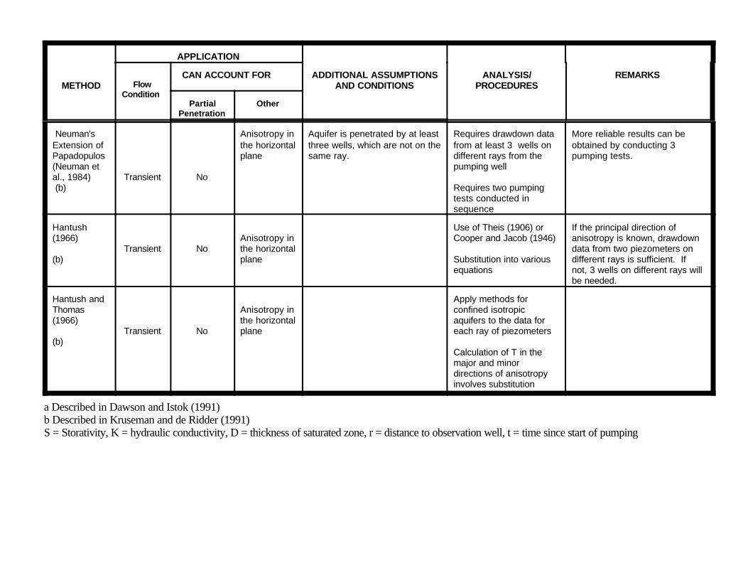
APPLICATION
METHOD FlowCondition
CAN ACCOUNT FOR
ADDITIONAL ASSUMPTIONSAND CONDITIONS
ANALYSIS/PROCEDURES
REMARKS
PartialPenetration
Other
Neuman'sExtension ofPapadopulos(Neuman etal., 1984) (b)
Transient No
Anisotropy inthe horizontalplane
Aquifer is penetrated by at leastthree wells, which are not on thesame ray.
Requires drawdown datafrom at least 3 wells ondifferent rays from thepumping well
Requires two pumpingtests conducted insequence
More reliable results can beobtained by conducting 3pumping tests.
Hantush(1966)
(b)Transient No
Anisotropy inthe horizontalplane
Use of Theis (1906) orCooper and Jacob (1946)
Substitution into variousequations
If the principal direction ofanisotropy is known, drawdowndata from two piezometers ondifferent rays is sufficient. Ifnot, 3 wells on different rays willbe needed.
Hantush andThomas(1966)
(b)Transient No
Anisotropy inthe horizontalplane
Apply methods forconfined isotropicaquifers to the data foreach ray of piezometers
Calculation of T in themajor and minordirections of anisotropyinvolves substitution
a Described in Dawson and Istok (1991) b Described in Kruseman and de Ridder (1991)S = Storativity, K = hydraulic conductivity, D = thickness of saturated zone, r = distance to observation well, t = time since start of pumping

Table 4.9 Multiple-well, Constant discharge pumping tests, leaky aquifers.
GENERAL ASSUMPTIONS1. The aquifer is leaky.2. The aquifer and aquitard have seemingly infinite and areal extent.3. The aquifer and aquitard are homogeneous, isotropic (unless noted), and of uniform thickness over the area influenced by the test.4. Prior to pumping, the piezometric surface and the water table are horizontal over the area that will be influenced by the test.5. The well penetrates the entire thickness of the aquifer and thus receives water by horizontal flow (unless noted).6. The flow in the aquitard is vertical.7. The drawdown in the unpumped aquifer (or aquitard) is negligible.8. Ground water flow can be described by Darcy's Law.
Additional assumptions for transient conditions:9.Water removed from storage in the aquifer and the water supplied by leakage from the aquitard is discharged instantaneously with decline of head.10. The diameter of the well is very small, i.e., the storage in the well can be neglected.
CAN ACCOUNT FOR
METHODFlow
Conditions Partial
PenetrationOther ADDITIONAL
ASSUMPTIONS ANDCONDITIONS
ANALYSIS/PROCEDURES
REMARKS
DeGlee (1930 &1951)
(b)
steadystate
NoL > 3D: where Lrepresents a leakagefactor and D is thesaturated thickness ofthe aquifer
Substitution intoequations
Hantush (1960) (b)
Transient No
Takes into accountstorage changes inthe aquitard
The aquitard iscompressible, i.e., thechanges in the aquitardstorage are appreciable
t < S ) D )
10K )
Type curve analysis
Generally is Theisequation plus an errorfunction
Only the early-timedrawdown should beused to satisfy theassumption that thedrawdown in theaquitard is negligible
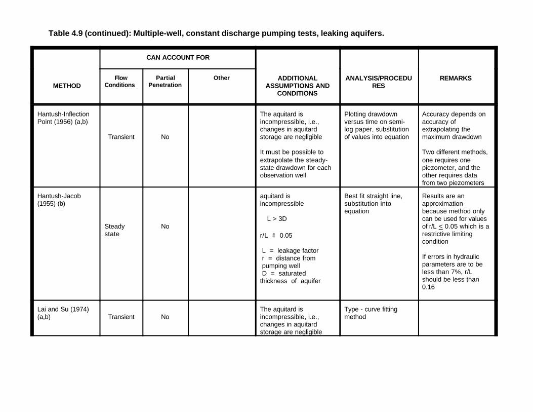
Table 4.9 (continued): Multiple-well, constant discharge pumping tests, leaking aquifers.
CAN ACCOUNT FOR
METHODFlow
Conditions Partial
PenetrationOther ADDITIONAL
ASSUMPTIONS ANDCONDITIONS
ANALYSIS/PROCEDURES
REMARKS
Hantush-InflectionPoint (1956) (a,b)
Transient No
The aquitard isincompressible, i.e.,changes in aquitardstorage are negligible
It must be possible toextrapolate the steady-state drawdown for eachobservation well
Plotting drawdownversus time on semi-log paper, substitutionof values into equation
Accuracy depends onaccuracy ofextrapolating themaximum drawdown
Two different methods,one requires onepiezometer, and theother requires datafrom two piezometers
Hantush-Jacob(1955) (b)
Steadystate
No
aquitard isincompressible
L > 3D
r/L # 0.05
L = leakage factor r = distance from pumping well D = saturatedthickness of aquifer
Best fit straight line,substitution intoequation
Results are anapproximationbecause method onlycan be used for valuesof r/L < 0.05 which is arestrictive limitingcondition
If errors in hydraulicparameters are to beless than 7%, r/Lshould be less than0.16
Lai and Su (1974)(a,b) Transient No
The aquitard isincompressible, i.e.,changes in aquitardstorage are negligible
Type - curve fittingmethod
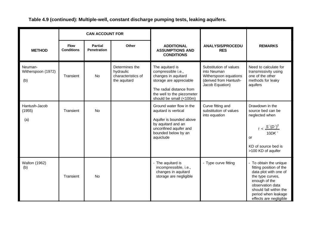
Table 4.9 (continued): Multiple-well, constant discharge pumping tests, leaking aquifers.
CAN ACCOUNT FOR
METHODFlow
Conditions Partial
PenetrationOther ADDITIONAL
ASSUMPTIONS ANDCONDITIONS
ANALYSIS/PROCEDURES
REMARKS
t < S )(D ))2
10DK )
Neuman-Witherspoon (1972)
(b)Transient No
Determines thehydrauliccharacteristics ofthe aquitard
The aquitard iscompressible i.e.,changes in aquitardstorage are appreciable
The radial distance fromthe well to the piezometershould be small (<100m)
Substitution of valuesinto NeumanWitherspoon equations(derived from Hantush-Jacob Equation)
Need to calculate fortransmissivity usingone of the othermethods for leakyaquifers
Hantush-Jacob(1955)
(a)
Transient NoGround water flow in theaquitard is vertical
Aquifer is bounded aboveby aquitard and anunconfined aquifer andbounded below by anaquiclude
Curve fitting andsubstitution of valuesinto equation
Drawdown in thesource bed can beneglected when
or
KD of source bed is>100 KD of aquifer
Walton (1962) (b)
Transient No
- The aquitard isincompressible, i.e.,changes in aquitardstorage are negligible
- Type curve fitting - To obtain the uniquefitting position of thedata plot with one ofthe type curves,enough of theobservation datashould fall within theperiod when leakageeffects are negligible
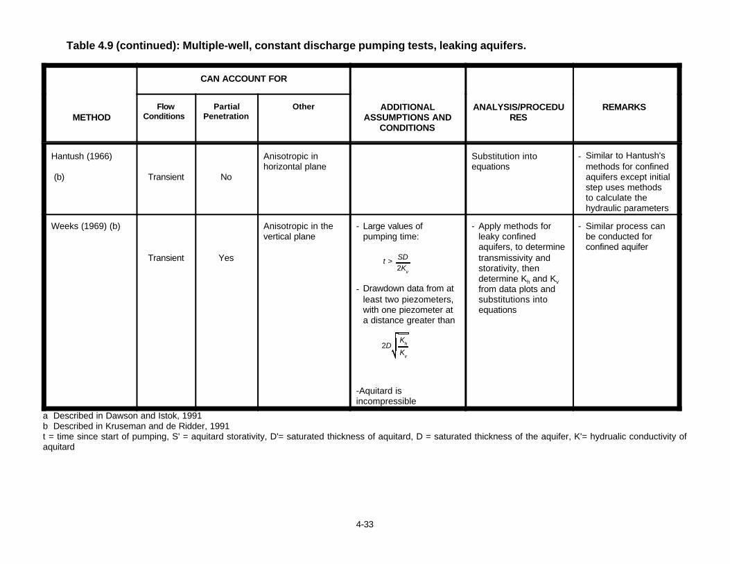
Table 4.9 (continued): Multiple-well, constant discharge pumping tests, leaking aquifers.
CAN ACCOUNT FOR
METHODFlow
Conditions Partial
PenetrationOther ADDITIONAL
ASSUMPTIONS ANDCONDITIONS
ANALYSIS/PROCEDURES
REMARKS
4-33
t > SD2Kv
Hantush (1966)
(b) Transient No
Anisotropic inhorizontal plane
Substitution intoequations
- Similar to Hantush'smethods for confinedaquifers except initialstep uses methodsto calculate thehydraulic parameters
Weeks (1969) (b)
Transient Yes
Anisotropic in thevertical plane
- Large values ofpumping time:
- Drawdown data from atleast two piezometers,with one piezometer ata distance greater than
2DKh
Kv
-Aquitard isincompressible
- Apply methods forleaky confinedaquifers, to determinetransmissivity andstorativity, thendetermine Kh and Kvfrom data plots andsubstitutions intoequations
- Similar process canbe conducted forconfined aquifer
a Described in Dawson and Istok, 1991b Described in Kruseman and de Ridder, 1991t = time since start of pumping, S' = aquitard storativity, D'= saturated thickness of aquitard, D = saturated thickness of the aquifer, K'= hydrualic conductivity ofaquitard
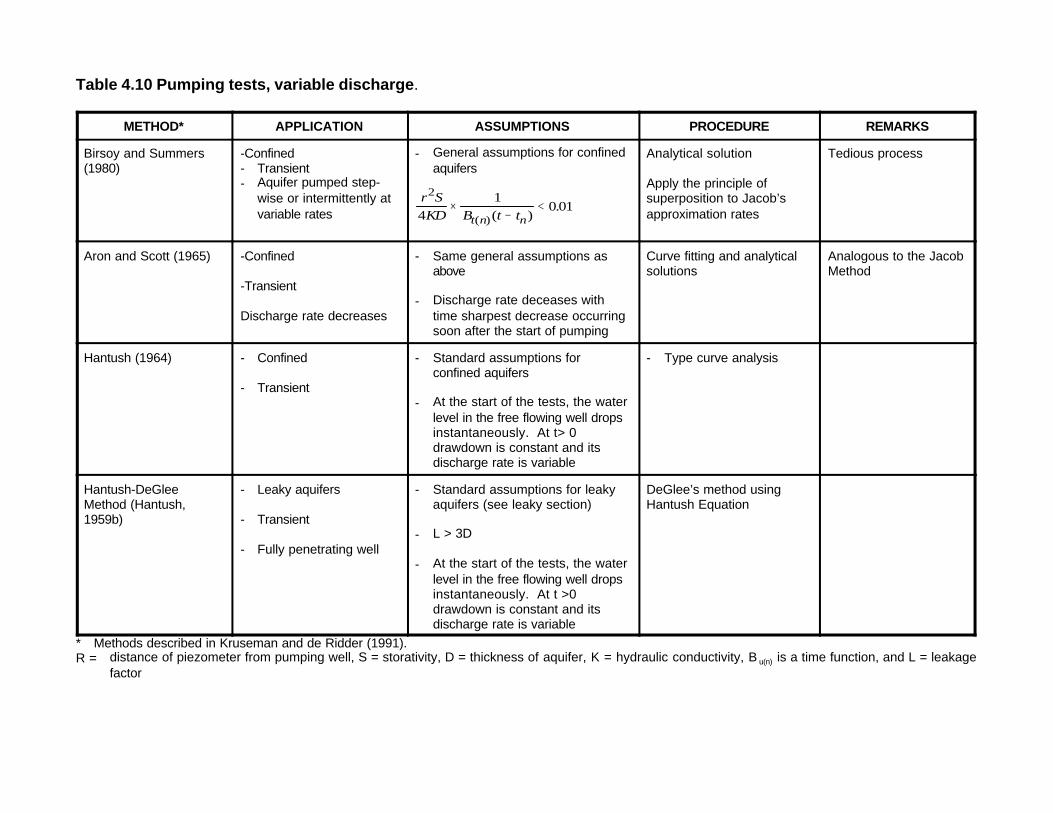
Table 4.10 Pumping tests, variable discharge.
METHOD* APPLICATION ASSUMPTIONS PROCEDURE REMARKS
Birsoy and Summers(1980)
-Confined- Transient- Aquifer pumped step-
wise or intermittently atvariable rates
- General assumptions for confinedaquifers
r SKD B t tt n n
2
41
0 01×−
<( )( )
.
Analytical solution
Apply the principle ofsuperposition to Jacob’sapproximation rates
Tedious process
Aron and Scott (1965) -Confined
-Transient
Discharge rate decreases
- Same general assumptions asabove
- Discharge rate deceases withtime sharpest decrease occurringsoon after the start of pumping
Curve fitting and analyticalsolutions
Analogous to the JacobMethod
Hantush (1964) - Confined
- Transient
- Standard assumptions forconfined aquifers
- At the start of the tests, the waterlevel in the free flowing well dropsinstantaneously. At t> 0drawdown is constant and itsdischarge rate is variable
- Type curve analysis
Hantush-DeGleeMethod (Hantush,1959b)
- Leaky aquifers
- Transient
- Fully penetrating well
- Standard assumptions for leakyaquifers (see leaky section)
- L > 3D
- At the start of the tests, the waterlevel in the free flowing well dropsinstantaneously. At t >0drawdown is constant and itsdischarge rate is variable
DeGlee’s method usingHantush Equation
* Methods described in Kruseman and de Ridder (1991).R = distance of piezometer from pumping well, S = storativity, D = thickness of aquifer, K = hydraulic conductivity, B u(n) is a time function, and L = leakage
factor

2 Methods are described in Kruseman and de Ridder, 1991.
4-35
Table 4.11 Methods of analysis for pumping tests with special conditions.
CONDITION FLOW AQUIFER
TYPEMODELS &SOURCES2
One or more recharge boundaries Steady State Confined orUnconfined
Dietz (1943)
One or more straight rechargeboundaries
UnsteadyState
Confined orUnconfined
Stallman (in Ferris etal., 1962)
One recharge boundary UnsteadyState
Confined orUnconfined
Hantush (1959a)
Aquifer bounded by two fullypenetrating boundaries
UnsteadyState
Leaky orConfined
Vandenberg (1976and 1977)
Wedge shaped aquifer UnsteadyState
Confined Hantush (1962)
Water table slopesSteady State Unconfined Culmination Point
Method (Huisman,1972)
UnsteadyState
Unconfined Hantush (1964)
Two layered aquifer, unrestrictedcross flow
Pumping well does not penetrateentire thickness
UnsteadyState
Confined Javandel-Witherspoon (1983)
Leaky two-layered aquifer,separated by aquitard with cross-flow across aquitard
Steady State Leaky Bruggeman (1966)
Large diameter well UnsteadyState
Confined Papadopulos (1967),Papadopulos andCooper (1967)
Large diameter well UnsteadyState
Unconfined Boulton andStreltsova, (1976)
4-36
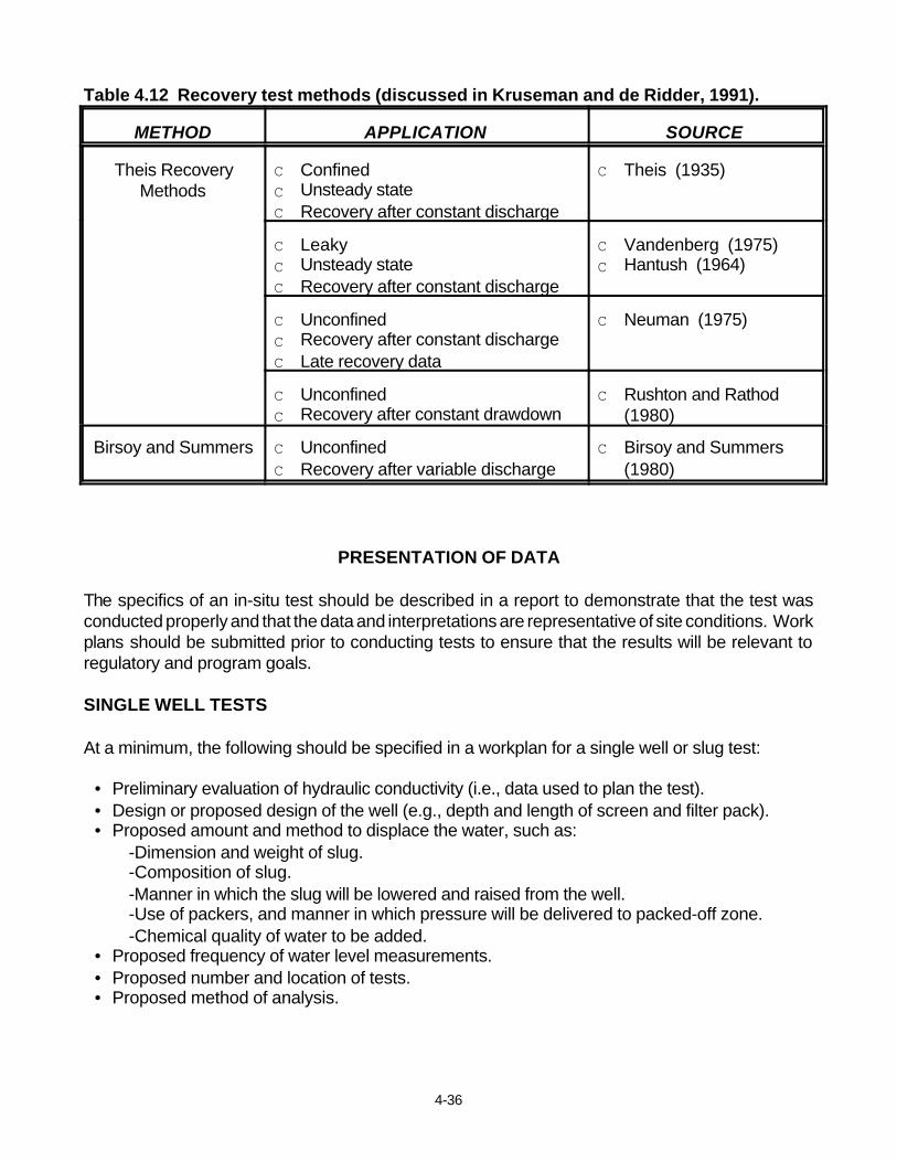
Table 4.12 Recovery test methods (discussed in Kruseman and de Ridder, 1991).
METHOD APPLICATION SOURCE
Theis RecoveryMethods
C ConfinedC Unsteady stateC Recovery after constant discharge
C Theis (1935)
C LeakyC Unsteady stateC Recovery after constant discharge
C Vandenberg (1975)C Hantush (1964)
C UnconfinedC Recovery after constant dischargeC Late recovery data
C Neuman (1975)
C Unconfined C Recovery after constant drawdown
C Rushton and Rathod (1980)
Birsoy and Summers C UnconfinedC Recovery after variable discharge
C Birsoy and Summers (1980)
PRESENTATION OF DATA
The specifics of an in-situ test should be described in a report to demonstrate that the test wasconducted properly and that the data and interpretations are representative of site conditions. Workplans should be submitted prior to conducting tests to ensure that the results will be relevant toregulatory and program goals.
SINGLE WELL TESTS
At a minimum, the following should be specified in a workplan for a single well or slug test:
• Preliminary evaluation of hydraulic conductivity (i.e., data used to plan the test).• Design or proposed design of the well (e.g., depth and length of screen and filter pack).• Proposed amount and method to displace the water, such as:
-Dimension and weight of slug.-Composition of slug.-Manner in which the slug will be lowered and raised from the well.-Use of packers, and manner in which pressure will be delivered to packed-off zone.-Chemical quality of water to be added.
• Proposed frequency of water level measurements.• Proposed number and location of tests. • Proposed method of analysis.

4-37
To provide adequate documentation that the test was conducted and interpreted correctly, thefollowing should be provided in a report:
• The design and implementation of the test (workplan content items as specified above).• All raw data (including type curves, if used).• Sample calculations.• Any field conditions or problems noted during the test that may influence the results. • An evaluation and interpretation of the data (relating it to overall site conditions).
MULTIPLE WELL PUMPING TESTS
At a minimum, the following should be provided in a workplan for a conventional multiple wellpumping test:
• Preliminary evaluation of hydrogeologic conditions, including all data used to plan and designthe test.
• Proposed test and rationale for design, including but not limited to:
- Geologic zone into which the pumping well is completed (i.e. areal extent, thickness,lateral and vertical extent).
- Pumping well construction (justification should be provided if the well screen is partiallypenetrating).
- Duration of pumping.
- Rate of pumping and method for determination.
- Location of all proposed observation wells.
- Geologic zone(s) to be monitored (including depths, thickness, spatial relationship to thepumped zone).
- Observation well construction.
- Method of water level measurements (for each well).
- Methods for gathering data used to correct drawdown and establishment of existingtrends in water levels.
- Method of data analysis.
- Procedures for the discharge of pumped water.

4-38
After completion of a pumping test, the following should be included in a report to document that thetest was conducted and interpreted correctly:
• Specific design of the test (workplan content items as specified above), includingmodifications from the planned configuration and rationale for any deviations.
• Date and time pumping began and ended.
• Raw data, including water level measurements, time of measurement in minutes afterpumping started or ended, drawdown, pumping rates, etc. All data should be expressedin consistent units.
• Data plots and type curves, if used. All graphs and data plots should be labeled clearly.
• Calculations.
• Comments noting any external events (e.g., change in weather patterns, passage of trainor heavy machinery).
• Data plots, graphs, and equations used to determine drawdown corrections.
• Data analysis method, including assumptions, limitations and references.
• Interpretation of the data using both results of the test and other available hydrogeologicinformation.
4-39
REFERENCES
Anonymous, 1964. Steady Flow of Groundwater Towards Wells. Proc. Comm. Hydrology.Research TNO No.10. Cited in Kruseman and de Ridder, 1991.
Aron, G. and V. H. Scott. 1965. Simplified Solution For Decreasing Flow Into Wells. AmericanSociety of Civil Engineers Proceedings. Vol. 91, No. HY5, pp. 1-12.
ASTM Method D4044-91. 1992. Standard Test Method (Field Procedure) for InstantaneousChange in Head (Slug Tests) for Determining Hydraulic Properties of Aquifers. Annual Bookof American Society for Testing Materials Standards. Philadelphia, Pennsylvania. Vol. 04.08,pp. 609-611.
ASTM, Method D4104-91. 1992. Standard Test Method (Analytical Procedure) for DeterminingTransmissivity of Nonleaky Confined Aquifers by Overdamped Well Response to InstantaneousChange in Head (Slug Test). Annual Book of American Society for Testing MaterialsStandards. Philadelphia, Pennsylvania. Vol. 04.08, pp. 622-625.
ASTM, Method D4105-91. 1992. Standard Test Method (Analytical Procedure) for DeterminingTransmissivity and Storage Coefficient of Nonleaky Confined Aquifers by the Modified TheisNonequilibrium Method. Annual Book of American Society for Testing Materials Standards.Philadelphia, Pennsylvania. Vol. 04.08, pp. 626-630.
ASTM, Method D4106-91. 1992. Standard Test Method (Analytical Procedure) for DeterminingTransmissivity and Storage Coefficient of Nonleaky Confined Aquifers by the Modified TheisNonequilibrium Method. Annual Book of American Society for Testing Materials Standards.Philadelphia, Pennsylvania. Vol. 04.08, pp. 631-635.
ASTM, Method D4043-91. 1992. Standard Guide for the Selection of Aquifer-Test Methods inDetermining the Hydraulic Properties by Well Techniques. Annual Book of American Societyfor Testing Materials Standards. Philadelphia, Pennsylvania. Vol. 04.08, pp. 604-608.
ASTM, Method D4750-87. 1992. Standard Test Method for Determining Subsurface Liquid Levelsin a Borehole or Monitoring Well (Observation Well). Annual Book of American Society forTesting Materials Standards. Philadelphia, Pennsylvania. Vol. 04.08, pp. 1021-1060.
Birsoy, Y. K. and W. K. Summers. 1980. Determination of Aquifer Parameters From Step Testsand Intermittent Pumping Data. Ground Water. Vol. 18, No. 2, pp. 137-146.
Black, J. H. 1978. The Use of Slug Tests in Ground Water Investigations. Water Services. pp.174-178.
Boonstra, J. and N. A. de Ridder. 1981. Numerical Modelling of Ground Water Basins.International Institute for Land Reclamination and Improvement. Wageningen, The Netherlands.
4-40
Boulton, N. S. and T. D. Streltsova. 1976. The Drawdown Near an Abstraction of Large DiameterUnder Non-Steady State Conditions in Unconfined Aquifers. Journal of Hydrology. Vol. 30, pp.29-46.
Bouwer, H. and R. C. Rice. 1976. A Slug Test For Determining Hydraulic Conductivity ofUnconfined Aquifers with Complete or Partially Penetrating Wells. Water Resources Research.Vol. 12, No. 3, pp. 423-428.
Bouwer, H. 1989. The Bouwer and Rice Slug Test--An Update. Ground Water. Vol. 27, No. 3, pp.304-309.
Bredehoeft, J. D. and S. S. Papadopulos. 1980. A Method for Determining Hydraulic Propertiesof Tight Formations. Water Resources Research. Vol. 16, No. 1, pp. 233-238.
Bruggeman, G. A. 1966. Analyse van de Bodemconstanten in een Grondpakket, Bestaande UitTwee of Meer Watervoerende Lagen Gescheiden door Semi-Permeabele Lagen. UnpublishedResearch Paper. Cited in Kruseman and de Ridder, 1991.
Chirlin, G. R. 1990. The Slug Test: The First Four Decades. Ground Water Management.Proceedings of the 1990 Cluster Conference. National Water Well Association. Columbus,Ohio. pp. 365-381.
Cooper, H. H., J. D. Bredehoeft, and I. S Papadopulos. 1967. Response of a Finite-Diameter Wellto an Instantaneous Charge of Water. Water Resources Research. Vol. 3, No. 1, pp. 263-269.
Cooper, H. H. and C. E. Jacob. 1946. A Generalized Graphical Method for Evaluating FormationConstants and Summarizing Well Field History. Transactions of the American GeophysicalUnion. Vol. 24, No. 4, pp. 526-534.
Dalton, M. G., B. E. Huntsman, and K. Bradbury. 1991. Acquisition and Interpretation of Water-Level Data. In: D. M. Nielsen (editor), Practical Handbook of Ground-Water Monitoring. LewisPublishers, Inc. Chelsea, Michigan. pp. 367-395.
Dawson, K. and J. D. Istok. 1991. Aquifer Testing, Design and Analysis of Pumping and SlugTests. Lewis Publishers, Inc. Chelsea, Michigan.
De Glee, G. J. 1930. Over Grondwaterstromingen bij Wateronttrekking Door Middel Van Putten.Thesis. J. Waltman, Delft (The Netherlands). Cited in Kruseman and de Ridder (1991).
De Glee, G. J. 1951. Berekeningsmethoden voor de Winning van Grondwater. In:Drinkwatervoorziening, 3e Vacantiecursus: 38-80 Moorman's Periodieke pers. The Hague.Cited in Kruseman and de Ridder, 1991.
Dietz, D. N. 1943. De Toepassing van Invloedsfuncties bij het Berekenen van de Verlaging vanhet Grondwater ten Gevolge van Wateronttrekking. Water. Vol. 27(6), pp. 51-54. Cited inKruseman and de Ridder, 1991.
4-41
Driscoll, F. G. (editor). 1986. Groundwater and Wells. Second Edition. Wheelabrator EngineeredSystems-Johnson screens. St. Paul, Minnesota.
Ferris, J. G., D. B. Knowles, R. H. Brown, and R. W. Stallman. 1962. Theory of Aquifer Tests. U.S.Geological Survey, Water-Supply Paper 1536E.
Hantush, M. S. 1956. Analysis of Data From Pumping Tests in Leaky Aquifers. Transactions ofthe American Geophysical Union. Vol. 37, No. 6, pp. 702-714.
Hantush, M. S. 1959a. Analysis of Data From Pumping Well Near a River. Journal of GeophysicalResearch. Vol. 94, pp. 1921-1923.
Hantush, M. S. 1959b. Non-Steady Flow to Flowing Wells in Leaky Aquifers. Journal ofGeophysical Research. Vol. 64, No. 8, pp. 1043-1052.
Hantush, M. S. 1960. Modification of the Theory of Leaky Aquifers. Journal of GeophysicalResearch. Vol.65, No. 11, pp. 3713-3725.
Hantush, M. S. 1961a. Drawdown Around a Partially Penetrating Well. Journal of the HydraulicsDivision. Proceedings of the American Society of Civil Engineers. Vol. 87 (HY4), pp. 83-98.
Hantush, M. S. 1961b. Aquifer Tests on Partially Penetrating Wells. Journal of the HydraulicsDivision. Proceedings of the American Society of Civil Engineers. Vol. 87(HY5), pp. 172-195.
Hantush, M. S. 1962. Flow of Ground Water in Sands of Nonuniform Thickness-- Part 3, Flow toWells. Journal of Geophysical Research. Vol. 67, No. 4, pp. 1527-1534.
Hantush, M. S. 1964. Hydraulics of Wells. In: V. T. Chow (editor), Advances in Hydrosciences.Vol. 1. Academic Press. London and New York. pp. 281-442.
Hantush, M. S. 1966. Analysis of Data From Pumping Tests In Anisotropic Aquifers. Journal ofGeophysical Research. Vol. 71, No. 2, pp. 421-426.
Hantush, M. S. and C. E. Jacob. 1955. Non-Steady State Radial Flow in an Infinite Leaky Aquifer.Transactions of the American Geophysical Union. Vol. 36, No. 1, pp. 95-100.
Hantush, M. S. and R. G. Thomas. 1966. A Method for Analyzing a Drawdown Test in Anisotropic
Aquifers. Water Resources Research. Vol. 2, No. 2, pp. 281-285.
Huisman, L. 1972. Groundwater Recovery. MacMillan.
Hvorslev, M. J. 1951. Time Lag and Soil Permeability in Groundwater Observation. U.S. ArmyCorps of Engineers, Waterways Experiment Station. Bulletin No. 36. Vicksburg, Mississippi.
Jacob, C. E. 1944. Notes on Determining Permeability by Pumping Tests Under Water TableConditions. U.S. Geological Survey. Open file report.
4-42
Jacob, C. E. and S. W. Lohman. 1952. Non-Steady Flow to a Well of Constant Drawdown in anExtensive Aquifer. Transactions of the American Geophysical Union. Vol. 33, pp. 559-569.
Javandel, I. and R. A. Witherspoon. 1983. Analytical Solution of a Partially Penetrating Well in aTwo-Layer Aquifer. Water Resources Research. Vol 19., pp. 567-578.
Kruseman, G. P. and de Ridder, N. A. 1991. Analysis and Evaluation of Pumping Test Data.Second Edition. International Institute for Land Reclamation and Improvement (ILRI) Publication47. Wageningen, The Netherlands.
Lai, R. Y. S. and C. W. Su. 1974. Nonsteady Flow to a Large Diameter Well in a Leaky Aquifer.Journal of Hydrology. Vol. 22. pp. 333-345.
Lohman, S. W. 1972. Groundwater Hydraulics. U.S. Geological Survey Professional Paper 708.United States Government Printing Office. Washington, D.C.
Neuman, S. P. 1972. Theory of Flow in Unconfined Aquifers Considering Delayed Response ofthe Water Table. Water Resources Research. Vol. 8, No 4, pp. 1031-1045.
Neuman, S. P. 1974. Effects of Partial Penetration on Flow in Unconfined Aquifers ConsideringDelayed Gravity Response. Water Resources Research. Vol. 10, No 2, pp. 303-312.
Neuman, S. P. 1975. Analysis of Pumping Test Data From Anisotropic Unconfined AquifersConsidering Delayed Gravity Response. Water Resources Research. Vol. 11, No, 2, pp. 329-342.
Neuman, S. P. 1979. Perspective on 'Delayed Yield'. Water Resources Research. Vol. 15, No.4, pp. 899-908.
Neuman, S. P. and P. A. Witherspoon. 1972. Field Determination of the Hydraulic Properties ofLeaky Multiple Aquifer Systems. Water Resources Research. Vol. 8, No. 5, pp. 1284-1298.
Neuman, S. P., G. R. Walter, H. W. Bentley, J. J. Ward and D. D. Gonzalez. 1984. Determinationof Horizontal Anisotropy With Three Wells. Ground Water. Vol. 22, No. 1, pp. 66-72.
Orient, J. P., A. Nazar and R.C. Rice. 1987. Vacuum and Pressure Test Methods for EstimatingHydraulic Conductivity. Ground Water Monitoring Review. Vol. 7, No. 1, pp. 49-50.
Osborne, P. S. 1993. Suggested Operating Procedures for Aquifer Pumping Tests. U.S.EPA.Office of Research and Development, Office of Solid Waste. EPA/540/S-93/503.
Papadopulos, I. S. 1965. Nonsteady flow to a well in a finite anisotropic aquifer. InternationalAssociation of Scientific Hydroglogy Symposium. American Water Resources Assoc. Proc.No. 4, pp. 157-168.
Papadopulos, I. S. 1967. Drawdown Distribution Around a Large Diameter Well. Symposium onGroundwater Hydrology. Proceedings of American Water Resources. No. 4, pp. 157-168.
4-43
Papadopulos, I. S. and H. H. Cooper. 1967. Drawdown in Large Diameter Wells. WaterResources Research. Vol. 3, No. 1, pp. 241-244.
Rushton, K. R. and K. S. Rathod. 1980. Overflow Tests Analyzed by Theoretical and NumericalMethods. Ground Water. Vol. 18, No. 1, pp. 61-69.
Rushton, K. R. and V. S. Singh. 1983. Drawdowns in Large-diameter Wells Due To DecreasingAbstraction Rates. Ground Water. Vol. 21, No. 6, pp. 671-677.
Sevee, J. 1991. Methods and Procedures for Defining Aquifer Parameters. In: D. M. Nielsen(editor), Practical Handbook of Ground-Water Monitoring. Lewis Publishers, Inc. Chelsea,Michigan. pp. 397-448.
Stallman, R. W. 1983. Aquifer-Test Design, Observation and Data Analysis: U.S. GeologicalSurvey Techniques of Water-Resource Investigations, Book 3, Chapter B1. United StatesGovernment Printing Office. Washington, D. C.
Streltsova, T. D. 1974. Drawdown in Compressible Unconfined Aquifer. Journal of the HydraulicsDivision. American Society of Civil Engineers. HYll, pp. 1601-1616.
Theis, C. V. 1935. The Relation Between the Lowering of the Piezometric Surface and the Rateand Duration of Discharge of a Well Using Groundwater Storage. Transactions of the AmericanGeophysical Union. Vol. 16, pp. 519-524.
Thiem, G. 1906. Hydrologische Methoden. Gebhardt. Leipzig. Cited in Kruseman and de Ridder,1991.
Uffink, G. J. M. 1984. Theory of the Oscillating Slug Test. National Institute for Public Health andEnvironmental Hygiene Bilthoven. Unpublished research report (in Dutch). Cited in Krusemanand de Ridder, 1991.
U.S. EPA. 1986. Saturated Hydraulic Conductivity, Saturated Leachate Conductivity and IntrinsicPermeability. In: Test Methods for Evaluating Solid Waste. SW846, Method 9100. Office ofSolid Waste and Emergency Response. U.S. Environmental Protection Agency. Washington,D.C.
Vandenberg, A. 1975. Determining Aquifer Coefficients From Residual Drawdown Data. WaterResources Research. Vol. 11, pp. 1025-1028.
Vandenberg, A. 1976. Tables and Types Curves for Analysis of Pumping Tests in Leaky Parallel-Channel Aquifers. Technical Bulletin No. 96. Inland Waters Directorate, Water ResourceBranch. Ottawa (Canada).
Vandenberg, A. 1977. Type Curve Analysis of Pump Tests in Leaky Strip Aquifers. Journal ofHydrology. Vol. 33, pp. 15-26.
4-44
Van der Kamp, G. 1985. Brief Quantitative Quidelines for Design and Analysis of Pumping Tests.In: Hydrology in the Service of Man. Memoirs of the 18th Congress Intern. Assoc. Hydrogeol.Cambridge, Massachusetts. pp. 197-206
Walton, W. C. 1962. Selected Analytical Methods for Well and Aquifer Evaluation. Illinois StateWater Survey. Bulletin No. 49.
Walton, W. C. 1987. Groundwater Pumping Tests, Design and Analysis. Lewis Publishers, Inc.Chelsea, Michigan.
Weeks, E. P. 1969. Determining the Ratio of Horizontal to Vertical Permeability by Aquifer-TestAnalysis. Water Resources Research. Volume 5, pp. 196-214.
Worthington, P. F. 1981. Estimation of Transmissivity of Thin Leaky-Confined Aquifers fromSingle-Well Pumping Test. Journal of Hydrology. Vol. 49, pp. 19-30.


![Guide to Conducting Pumping Tests - B.C. … 4 ] HOW IS PUMPING RATE SELECTED? The well should be pumped at or above the intended pumping rate of the well and the well should not be](https://img.pdfslide.us/doc/110x75/5ccd45bc88c993de558dee0c/guide-to-conducting-pumping-tests-bc-4-how-is-pumping-rate-selected-the-well.jpg)