1

Pulsed laser ablation as a tool for in-situ balancing of rotating

parts

M. Stoesslein, D. A. Axinte*, A. Guillerna,

Rolls-Royce UTC in Manufacturing and On-Wing Technology, Faculty of Engineering, University of

Nottingham, UK

Abstract

The balancing of complex rotating systems is a challenging task as it may require repetitive

(dis)assembly to enable mass adjustments; thus, developing methods for in-situ dynamic balancing of

rotatives is regarded as a key technology enabler. In this context laser balancing with its high flexibility

in adjusting its firing frequency (to match that of the rotating part) and pulse energy (to vary the

material removal) could offer significant advantages from both precision and cost point of view.

In this paper a laser balancing system is developed to continuously remove material from a target part

in a controlled and automated manner. The amount of material ablated can be controlled by an

influence coefficient which is related to the change in vibration amplitude for a predefined amount of

pulses at a given operational balancing speed, material, and geometry of the rotative part. The

proposed system features a three-layered case-driven programmatic approach to optimize single-plane

balancing process duration in a fully automated system. This enables the use of prioritization to avoid

misfire and therefore, structural damage to the targeted part. Furthermore, the application allows the

component to be balanced to all common balancing grades as specified in the ISO 1940/1 standard.

Thus, validation trials involved balancing an Inconel 718 rotative to a preliminarily specified balancing

grade by extracting the acceleration signals using an IIR peak filter. A computer simulation

encompassing the rotor bearing state space system, a model of the laser and the adapted peak

detection algorithm, has been developed and used to validate the trials conducted. Henceforth, a

maximum deviation from the desired correction position of less than 1 mm has been recorded.

Moreover, it has been shown that the detection and correction of imbalances can be reliably achieved

by reducing the vibration level of a rotor from G 22.5 to G 19.5.

Keywords: laser balancing; pulsed laser ablation; control strategy

2

Nomenclature

Variable Unit Description

m kg Mass of the rig

mu kg Mass of the imbalance

np - Number of laser pulse

ml kg/np Mass removal per pulse

L m Length of the shaft

Z1 m Distance from the ball bearing 1 to the horizontal

position of the imbalance

r m Radius of the imbalance

φ ° Radial position of the imbalance

ω rad/s Angular velocity of the rotor

t s Time of the simulation

td s Time delay between triggering a pulse and the laser

firing

kixx - Bearing i dynamic stiffness coefficient in x direction

kixy - Bearing i dynamic stiffness coefficient in xy direction

kiyx - Bearing i dynamic stiffness coefficient in yx direction

kiyy - Bearing i dynamic stiffness coefficient in y direction

cixx - Bearing i dynamic damping coefficient in x direction

cixy - Bearing i dynamic damping coefficient in xy direction

ciyx - Bearing i dynamic damping coefficient in yx direction

ciyy - Bearing i dynamic damping coefficient in y direction

i - 1, 2

kt - Threshold amplitude for peak identification

kw min rad Minimum period width

kw measured rad Measured period width

θ rad Position of rotor

k1 - Constant for signal threshold

k2 - Constant for minimum period width

k3 m/s2/np Calibration Constant

3

eper - Permissible specific unbalance

1. Introduction

Balancing has become an essential part of many manufacturing and maintenance processes in the

power turbine, defence, automobile and airplane industry; it contributes to the increase of the life cycle

and reliability of rotary components, while also decreasing wear and the overall noise level of the

system [1]. Negligence to balance rotatives can lead to malfunctioning, that is the common failure

modes being bending of the shaft, fatigue and failure in the bearing of the rotative. Balancing is a

standard process in many industries, especially in those related with high-speed applications.

Nevertheless, this relies on strict procedures that usually end-up in extensive idle times. Usually a

balancing machine first determines the position and the mass of the imbalance. Then the imbalance is

either removed in a separate step using removal techniques, or it can be counterbalanced by the

addition of mass opposite to the angular location of the imbalance. Of particular difficulty is the addition

and removal of small masses, which is a commonly required for fine balancing and is time consuming

as it requires manual interaction.

During the last decades the challenges have become ever more complex requiring balancing

components/assemblies without disruption to the setpus and henceforth, there is a need for in-situ

balancing machines capable of detecting imbalances in the magnitude of G 0.4. Those advances can

mainly be attributed towards the rapid digitalization of machines. In 1974 Schenk pioneered the first

computer controlled balancing machine. Consequently, in the early 80s the first micro-processor based

balancing machine revolutionized the market enabling the easy balancing of dynamic unbalances [2].

Engine industries require the balancing of whole assemblies, thus, challenging existing strategies.

Hence, there is a need to provide balancing processes capable of both operating with little space for

machining equipment and creating no waste, which can damage adjacent components in the assembly

during the material removal process [3]. The topic of in-situ balancing has been the area of active

research over the past years, especially in regards of active magnetic bearing (AMB) balancing [4].

In this respect, NASA [5] has come up with a novel approach: spray automated balancing; this is a

solution to control material deposition onto a rotating component and therefore, avoid damage to

other parts of the assembly due to waste material. Nevertheless, spraying especially needs to ensure

high bond strength and appropriate surface finish. However, due to the size of the spraying gun this

method is likely to be unsuitable for in-situ balancing where access to balancing areas is restricted due

to space being the limiting factor.

A concept that can overcome those issues is laser balancing. The conceptualised idea to use lasers as a

removal method for balancing purposes was first discussed in the 60s [6]. The one of the advantages

4

of using Pulse Laser Ablation (PLA) is that the laser allows material removal (i.e. balancing) at high

rotational speeds with the limiting factor being their pulse duration; i.e. high pulse durations leads to a

low fluence, defined as energy per area, on the component and, therefore, little or no material removal.

Furthermore, fibre lasers, which can be bent by up to 90°, can be implemented in systems with very

little space and, therefore, employed in highly complex systems for in-situ balancing. However, most

importantly, when applied correctly the pulse laser ablation can vaporize material locally; hence, it can

access the imbalances of targeted parts without causing damage to nearby components of the

assembly [7]. Research has shown that ablation on a range of metallic materials can be conducted with

minimal/no thermal alteration of metallurgical properties of the workpiece target material [8] by

operating below the damage threshold [9].

Although the idea of pulsed laser ablation balancing for gyroscopic assemblies and small turbines has

been commented by industrial technical briefs, there is no scientific article to explain in-depth the

working principles, challenges, and the associated systems to enable the implementation of such

approach for balancing larger rotating assemblies. This is needed for enabling larger material removal

(i.e. surfaces) and not “punctual” balancing as utilized for small rotating parts. This is a very limiting

factor especially when large structures need significant volume of material to be removed in particular

zones where they will not impart the service performance (e.g. aero engine, power turbines).

The idea of utilizing pulsed lasers for balancing purposes is driven by the need to minimize the balancing

operational time, while also achieving low level of imbalance. This paper [6] proposes a setup using a

triggering signal from a measuring sensor (e.g. accelerometer) to fire the laser in a particular angular

position of the rotating part. Furthermore, this setup includes a system to compensate for the delays

in firing (a Q-switched) laser by 0.7 ms to counteract for the pulse build up. However, due to the low

power output of the laser available and long pulse duration in the ms regime, which does not allow for

point ablation at high balancing speeds, Schultz [6] concluded that a laser balancing system would not

be economically viable. Furthermore, the reported system was unable to determine the position of the

imbalance without interaction of a user, which involved manual calculations of the imbalance position

and mass.

A NASA report [5] discussed a method for two-plane balancing of a flexible rotor to reduce operation

time and fully automate the process. The paper suggests the use of predefined balancing holes, which

would allow the laser to be inserted into the assembly to balance whenever needed without the need

to disassemble the system. This could imply that the method has “pre-defined” positions to fire the

laser and, therefore, could not be considered a fully flexible approach to perform this task on different

part geometries/surfaces without preliminary investigations. Furthermore, this report fails to discuss

the controls and methods required for this approach to work.

5

However, in the early 90s another attempt on laser balancing, this time with a more material focused

view, was reported. This [10] describes a pilot system designed to balance gas turbine engines and

features a high power Nd:YAG laser capable of delivering up 50 Joules per 1ms pulse. The experimental

system was capable of automatic balancing, however, the operator was required to select a calibration

file for the balancing to work. Although this is by far the most advanced laser balancing system

mentioned in literature, the paper fails to describe the mechatronics and control strategies utilized; so,

it could hardly be a base for further advancements in the field. Additionally, the implemented controls

only account for point ablation, a process at which the laser pulses at the exact location of the

imbalance effectively drilling a hole to remove material, which can damage the structural integrity of

complex geometry components and lead to reduced life time.

Therefore, although laser balancing could be an interesting academic problem with high applicative

impact, up to now limited number academic papers have been reported in relation to this particular

field.

Without information/theory on the mechatronics and control principles of such systems and how the

laser firing is synchronized with the part rotation, no significant development can be done in this field

to enable balancing of complex geometry components by removing truly 3D shapes.

This paper focuses on the optimum way of implementing laser balancing utilizing spot removal

technique with a modern fibre laser. Additionally, it explores the impact of implementing an IIR filter to

adjust for external disturbances. Ultimately, it is necessary to apply a more practical mechatronics

approach to understand the working of a laser balancing system and how to optimize it to meet the

specifications required by industry especially in the balancing of shafts and rotors for the turbine engine

industry.

2. An approach to in-situ balancing

One of the most common causes for vibration in machines are the imbalances acting alone or in

combination with other vibration issues like misalignment. On a perfectly radial aligned rotative

imbalances result in a centripetal force. In this paper it is assumed that the vibration is caused by a

‘heavy spot’ in a known plane (i.e. single plane balancing) of a rotative at a known constant radial

velocity. Thus, each time the imbalance passes through an arbitrary selected radial position it causes a

force acting in the opposite direction to the axis of the rotor bearing system. Hence, measuring the

acceleration at a given radial position will result in a sinusoidal wave with a frequency equal to the radial

velocity of the system, where the amplitude is directly proportional to the mass of the imbalance.

6

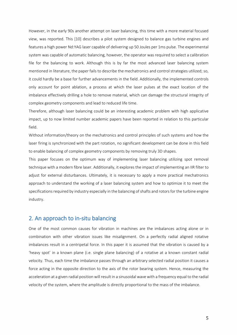
Figure 1 The laser balancing 3 step procedure, where f is the frequency: 1) Acquire data using the

accelerometer mounted above the ball bearing 2) Evaluation of the peak position and amplitude to

identify the imbalance location and mass 3) triggering of the laser to remove the imbalance using

PLA

PLA as a method to remove material offers distinct advantages to current removal techniques used in

industry (e.g. grinding, drilling etc.) since the removed material evaporates, and therefore waste

material cannot damage neighbouring components during in-situ balancing processes. Furthermore, it

allows the operator to adjust pulse energy, frequency and pulse duration to achieve effortless the

desired surface finish.

Thus, a methodology for detecting imbalances as well as removing such with a pulsed fibre laser

involving a three-step process was developed. The first stage encompasses the acquisition of the

acceleration as well as the encoder measurements of the balancing rig and the ‘matching’ of these

signals for further processing. In most balancing situations it is difficult or impossible to measure the

vibration at the source; therefore, it is usually measured at the rig on one or two horizontal positions

depending on whether the horizontal location of the imbalance is known. This paper assumes the

horizontal position to be known, and therefore requires only one accelerometer signal. However, the

method can easily be extended to account for the horizontal position, too. Secondly, the collected

acceleration signal is analysed for peaks identifying the radial location and mass of a potential residual

imbalance. Lastly, using the identified peak location, the laser is triggered to ablate the imbalance while

Peak Detection

Balancing Rig

Laser Triggering

Accelerometer

Motor &Encoder

Pulsed laser

f

f

7

the rotor system remains at operational velocity. The process is iterative and the steps are repeated

until the imbalance is below a user specified level.

Therefore, a rotor bearing state space model has been developed to assess the feasibility, accuracy and

process time of the in-situ PLA balancing methodology proposed. Figure 1 shows the three step iterative

process with the green dots representing the imbalance location and the red lines the physical

communication network. While only shown on a rig, the proposed methodology can also be applied to

in-situ balancing situation to avoid (dis)assembly costs. It can also be used to actively move imbalances

and hence, avoid removing material from critical surfaces of the component/assembly to be balanced.

3. Design of a model for imbalance estimation

In this section equations of the rotor bearing state space model are developed and presented,

additionally a detection method is developed to estimate single plane residual imbalances on an

arbitrary rotor rotating at a constant radial velocity, ω. The rotor is assumed to be rigid, the laser pulses

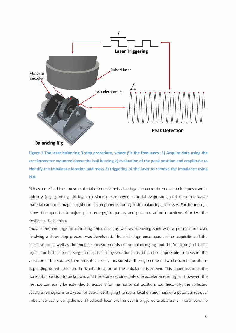
instant, and the bearings are assumed to exert no friction onto the rotative. Figure 2 shows the block

diagram of the complete laser balancing system.

Figure 2 The block diagram shows the control of the laser balancing process

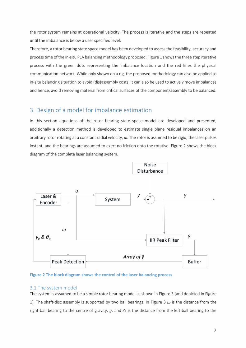
3.1 The system model The system is assumed to be a simple rotor bearing model as shown in Figure 3 (and depicted in Figure

1). The shaft-disc assembly is supported by two ball bearings. In Figure 3 L2 is the distance from the

right ball bearing to the centre of gravity, g, and Z1 is the distance from the left ball bearing to the

System

Noise Disturbance

IIR Peak Filter

yLaser & Encoder

u

ŷ

y++

Peak Detection BufferArray of ŷ

yp & θp

ω

8

imbalance mass, mu, at eccentricity e (i.e. radius of the imbalance). The rotor has a total length of L and

a constant angular velocity of ω. Each of the ball bearings has an internal stiffness coefficient, k, and

damping coefficient, c. L1 and Z2 are calculated correspondingly as shown

𝑳𝟐 = (𝑳 − 𝑳𝟏), 𝒁𝟐 = (𝑳 − 𝒁𝟏) ( 1 )

The linearized Eq. of the rotor bearing system [11] are given as

𝑴�� + (𝝎𝑮 + 𝑪)�� + 𝑲𝒒 = 𝑭 ( 2 )

where ω the constant radial velocity and F the force matrix of the centripetal acceleration force caused

by the imbalance mu. The horizontal, x, and vertical direction, y, of both bearings have been chosen as

the states, q, of the system as shown in Eq. ( 3 ) and Figure 3. The acceleration in the axial direction of

the shaft or z was neglected due to it being unnecessary for residual imbalance detection.

𝑞 = [

𝑥1

𝑦1

𝑥2

𝑦2

]

( 3 )

Figure 3 The rotor bearing system consisting of a shaft fixed by two ball bearings and a disk with

the imbalance mu added

M, G, C and K are the mass, gyroscopic, damping and stiffness matrices given as

𝑀 =

[

𝑚𝑙22 + 𝑖𝑡 0 𝑚𝑙1𝑙2 − 𝑖𝑡 0

0 𝑚𝑙22 + 𝑖𝑡 0 𝑚𝑙1𝑙2 − 𝑖𝑡

𝑚𝑙1𝑙2 − 𝑖𝑡 0 𝑚𝑙22 + 𝑖𝑡 0

0 𝑚𝑙1𝑙2 − 𝑖𝑡 0 𝑚𝑙22 + 𝑖𝑡 ]

( 4 )

L

Z1

L2

x1

y1

y2

x2

mu

m

g

k1yy c1yy

k1xx c1xx

k2xx c2xx

k2yy c2yy

ω r

9

𝐺 =

[

0 −𝑖𝑝 0 𝑖𝑝𝑖𝑝 0 −𝑖𝑝 0

0 𝑖𝑝 0 −𝑖𝑝−𝑖𝑝 0 𝑖𝑝 0 ]

( 5 )

𝐶 =

[ 𝑐1𝑥𝑥 𝑐1𝑥𝑦 0 0

𝑐1𝑦𝑥 𝑐1𝑦𝑦 0 0

0 0 𝑐2𝑥𝑥 𝑐2𝑥𝑦

0 0 𝑐2𝑦𝑥 𝑐2𝑦𝑦]

( 6 )

𝐾 =

[ 𝑘1𝑥𝑥 𝑘1𝑥𝑦 0 0

𝑘1𝑦𝑥 𝑘1𝑦𝑦 0 0

0 0 𝑘2𝑥𝑥 𝑘2𝑥𝑦

0 0 𝑘2𝑦𝑥 𝑘2𝑦𝑦]

( 7 )

𝑙𝑛 =

𝐿𝑛

𝐿, 𝑧𝑛 =

𝑍𝑛

𝐿, 𝑖𝑡 =

𝐼𝑥,𝑦

𝐿2, 𝑖𝑝 =

𝐼𝑝

𝐿2, 𝑛 = 1, 2

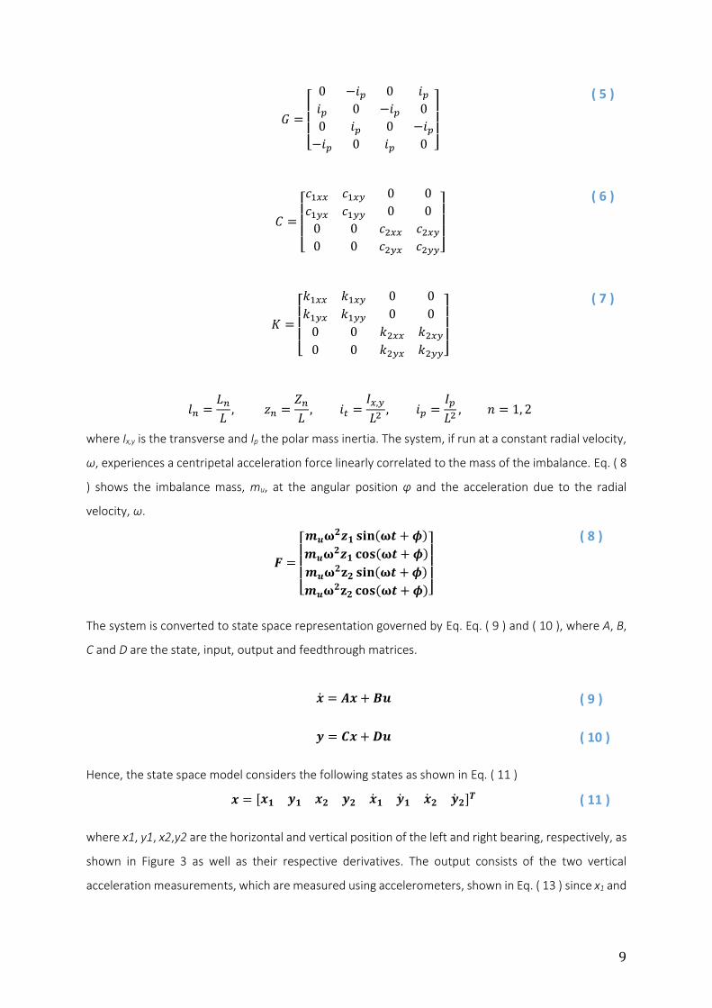
where Ix,y is the transverse and Ip the polar mass inertia. The system, if run at a constant radial velocity,

ω, experiences a centripetal acceleration force linearly correlated to the mass of the imbalance. Eq. ( 8

) shows the imbalance mass, mu, at the angular position φ and the acceleration due to the radial

velocity, ω.

𝑭 =

[ 𝒎𝒖𝛚𝟐𝒛𝟏 𝐬𝐢𝐧(𝛚𝒕 + 𝝓)

𝒎𝒖𝛚𝟐𝒛𝟏 𝐜𝐨𝐬(𝛚𝒕 + 𝝓)

𝒎𝒖𝛚𝟐𝐳𝟐 𝐬𝐢𝐧(𝛚𝒕 + 𝝓)

𝒎𝒖𝛚𝟐𝐳𝟐 𝐜𝐨𝐬(𝛚𝒕 + 𝝓)]

( 8 )

The system is converted to state space representation governed by Eq. Eq. ( 9 ) and ( 10 ), where A, B,

C and D are the state, input, output and feedthrough matrices.

�� = 𝑨𝒙 + 𝑩𝒖 ( 9 )

𝒚 = 𝑪𝒙 + 𝑫𝒖 ( 10 )

Hence, the state space model considers the following states as shown in Eq. ( 11 )

𝒙 = [𝒙𝟏 𝒚𝟏 𝒙𝟐 𝒚𝟐 ��𝟏 ��𝟏 ��𝟐 ��𝟐]𝑻 ( 11 )

where x1, y1, x2,y2 are the horizontal and vertical position of the left and right bearing, respectively, as

shown in Figure 3 as well as their respective derivatives. The output consists of the two vertical

acceleration measurements, which are measured using accelerometers, shown in Eq. ( 13 ) since x1 and

10

x2 are not measured as only one measurement which is necessary to determine the position and mass

of the imbalance.

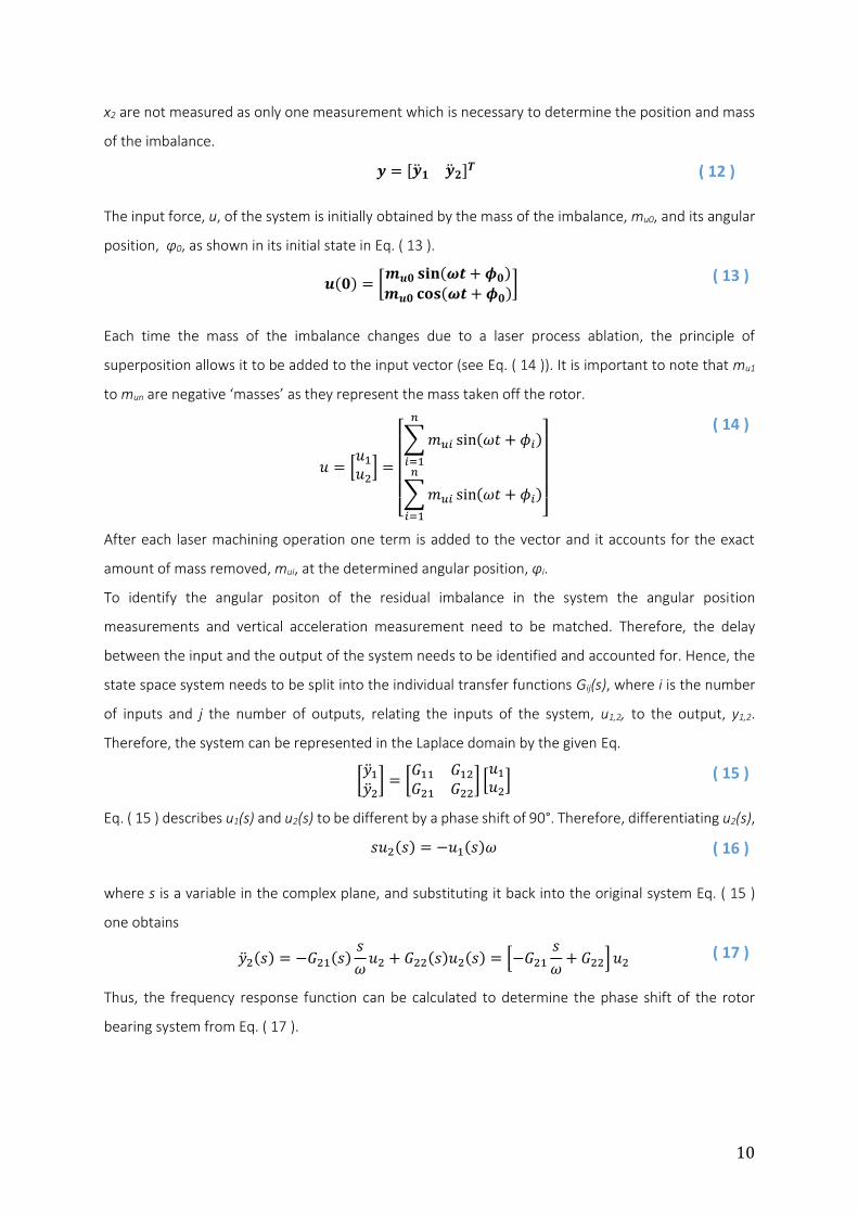
𝒚 = [��𝟏 ��𝟐]𝑻 ( 12 )

The input force, u, of the system is initially obtained by the mass of the imbalance, mu0, and its angular

position, φ0, as shown in its initial state in Eq. ( 13 ).

𝒖(𝟎) = [

𝒎𝒖𝟎 𝐬𝐢𝐧(𝝎𝒕 + 𝝓𝟎)

𝒎𝒖𝟎 𝐜𝐨𝐬(𝝎𝒕 + 𝝓𝟎)] ( 13 )

Each time the mass of the imbalance changes due to a laser process ablation, the principle of

superposition allows it to be added to the input vector (see Eq. ( 14 )). It is important to note that mu1

to mun are negative ‘masses’ as they represent the mass taken off the rotor.

𝑢 = [𝑢1

𝑢2] =

[ ∑𝑚𝑢𝑖 sin(𝜔𝑡 + 𝜙𝑖)

𝑛

𝑖=1

∑𝑚𝑢𝑖 sin(𝜔𝑡 + 𝜙𝑖)

𝑛

𝑖=1 ]

( 14 )

After each laser machining operation one term is added to the vector and it accounts for the exact

amount of mass removed, mui, at the determined angular position, φi.

To identify the angular positon of the residual imbalance in the system the angular position

measurements and vertical acceleration measurement need to be matched. Therefore, the delay

between the input and the output of the system needs to be identified and accounted for. Hence, the

state space system needs to be split into the individual transfer functions Gij(s), where i is the number

of inputs and j the number of outputs, relating the inputs of the system, u1,2, to the output, y1,2.

Therefore, the system can be represented in the Laplace domain by the given Eq.

[��1

��2] = [

𝐺11 𝐺12

𝐺21 𝐺22] [

𝑢1

𝑢2] ( 15 )

Eq. ( 15 ) describes u1(s) and u2(s) to be different by a phase shift of 90°. Therefore, differentiating u2(s),

𝑠𝑢2(𝑠) = −𝑢1(𝑠)𝜔 ( 16 )

where s is a variable in the complex plane, and substituting it back into the original system Eq. ( 15 )

one obtains

��2(𝑠) = −𝐺21(𝑠)𝑠

𝜔𝑢2 + 𝐺22(𝑠)𝑢2(𝑠) = [−𝐺21

𝑠

𝜔+ 𝐺22] 𝑢2 ( 17 )

Thus, the frequency response function can be calculated to determine the phase shift of the rotor

bearing system from Eq. ( 17 ).

11

3.2 Design of the IIR peak filter The acceleration data needs to be filtered in chunks, i.e. offline, to ensure the required accuracy and

precision in detecting the radial unbalance position. This is achieved by an Infinite Impulse Response

(IIR) digital filter rather than a Finite Impulse Response (FIR) filter due to memory restrictions on the

target and the high computational efficiency of the IIR filter. Hence, a 2nd order digital IIR peak filter

(i.e. the reverse of a notch filter) was implemented, with a varying peak depending on the rotational

speed of the rotor. A peak digital filter has a characteristic steep passband, i.e. it “peaks” for desired

frequency [12], which allows for a very clear filtered output signal at the desired frequency.

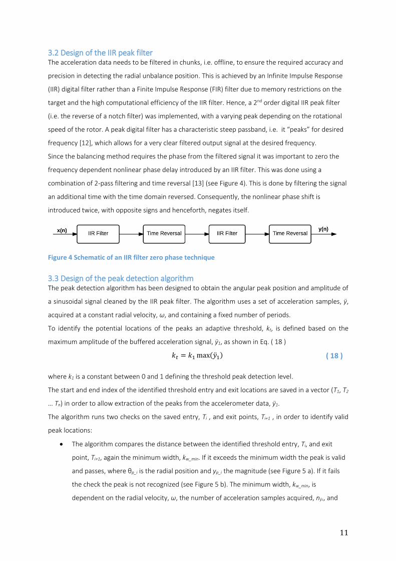
Since the balancing method requires the phase from the filtered signal it was important to zero the

frequency dependent nonlinear phase delay introduced by an IIR filter. This was done using a

combination of 2-pass filtering and time reversal [13] (see Figure 4). This is done by filtering the signal

an additional time with the time domain reversed. Consequently, the nonlinear phase shift is

introduced twice, with opposite signs and henceforth, negates itself.

Figure 4 Schematic of an IIR filter zero phase technique

3.3 Design of the peak detection algorithm The peak detection algorithm has been designed to obtain the angular peak position and amplitude of

a sinusoidal signal cleaned by the IIR peak filter. The algorithm uses a set of acceleration samples, y,

acquired at a constant radial velocity, ω, and containing a fixed number of periods.

To identify the potential locations of the peaks an adaptive threshold, kt, is defined based on the

maximum amplitude of the buffered acceleration signal, y1, as shown in Eq. ( 18 )

𝑘𝑡 = 𝑘1 max(��1) ( 18 )

where k1 is a constant between 0 and 1 defining the threshold peak detection level.

The start and end index of the identified threshold entry and exit locations are saved in a vector (T1, T2

… Tn) in order to allow extraction of the peaks from the accelerometer data, y1.

The algorithm runs two checks on the saved entry, Ti , and exit points, Ti+1 , in order to identify valid

peak locations:

The algorithm compares the distance between the identified threshold entry, Ti, and exit

point, Ti+1, again the minimum width, kw_min. If it exceeds the minimum width the peak is valid

and passes, where θp_i is the radial position and yp_i the magnitude (see Figure 5 a). If it fails

the check the peak is not recognized (see Figure 5 b). The minimum width, kw_min, is

dependent on the radial velocity, ω, the number of acceleration samples acquired, ny1, and

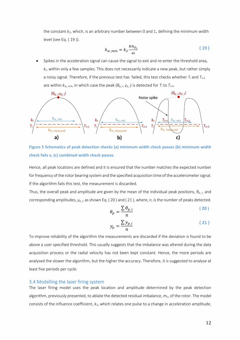
12

the constant k2, which, is an arbitrary number between 0 and 1, defining the minimum width

level (see Eq. ( 19 )).

𝑘𝑤_𝑚𝑖𝑛 = 𝑘2

𝜋𝑛��1

𝜔 ( 19 )

Spikes in the acceleration signal can cause the signal to exit and re-enter the threshold area,

kt, within only a few samples. This does not necessarily indicate a new peak, but rather simply

a noisy signal. Therefore, if the previous test has failed, this test checks whether Ti and Ti+2

are within kw_min, in which case the peak (θp_i, yp_i) is detected for Ti to Ti+3.

Figure 5 Schematics of peak detection checks (a) minimum width check passes (b) minimum width

check fails v, (c) combined width check passes

Hence, all peak locations are defined and it is ensured that the number matches the expected number

for frequency of the rotor bearing system and the specified acquisition time of the accelerometer signal.

If the algorithm fails this test, the measurement is discarded.

Thus, the overall peak and amplitude are given by the mean of the individual peak positions, θp_i, and

corresponding amplitudes, yp_i, as shown Eq. ( 20 ) and ( 21 ), where, n, is the number of peaks detected.

𝜃𝑝 =

∑𝜃𝑝_𝑖

𝑛

( 20 )

𝑦𝑝 =

∑𝑦𝑝_𝑖

𝑛

( 21 )

To improve reliability of the algorithm the measurements are discarded if the deviation is found to be

above a user specified threshold. This usually suggests that the imbalance was altered during the data

acquisition process or the radial velocity has not been kept constant. Hence, the more periods are

analysed the slower the algorithm, but the higher the accuracy. Therefore, it is suggested to analyse at

least five periods per cycle.

3.4 Modelling the laser firing system The laser firing model uses the peak location and amplitude determined by the peak detection

algorithm, previously presented, to ablate the detected residual imbalance, mu, of the rotor. The model

consists of the influence coefficient, k3, which relates one pulse to a change in acceleration amplitude,

13

and the removal mass per laser pulse, ml. Hence, the total amount of pulses, np, needed to remove the

residual imbalance, mu, is calculated as given in Eq. ( 22 ).

𝑛𝑝 =𝑦𝑝

𝑘3𝑚𝑙

( 22 )

The influence coefficient (as an average) was obtained by firing a high number of pulses (e.g. 1000) at

the target and divide the change in acceleration amplitude by the amount of pulses fired.

If the measured acceleration is above the defined threshold (i.e. the requested balancing grade)

material is removed.

4. Implementation of the proposed method

To validate the model established in section 3 a computer simulation has been developed and controller

has been programmed. This section details the adaption of the methodology required for a working

implementation into a hardware and software system.

4.1 Design of a computer simulation To verify the mathematical model developed above a three step discrete simulation has been

developed. The rig model has been estimated on basis of the model developed in section 3.1 using

system identification. The system identification was done using acceleration data acquired with a

known imbalance added onto the rotor. First, the rotor bearing model is simulated to fill up the buffer

(i.e. generate acceleration with some added noise and encoder measurements); secondly, the buffered

signals are analysed by the peak detection algorithm and the location of the imbalance as well as the

corresponding amplitude are determined. Lastly, the input of the system model (see Eq. ( 14 )) is

modified to account for the chosen amount of mass (based on the amplitude of the imbalance) ablated

due to the results from the peak detection analysis. This is repeated until the amplitude (which is related

to the balancing grade) is below the user-defined threshold (i.e. the specified balancing grade).

A script allows the user to configure all basic parameters like the shaft weight and the maximum laser

shots per cycle. Outputs of the simulation include a log of the detected imbalance mass and location

detailed with the correction response of the simulation, which is also graphically visualized.

Furthermore, a graph shows the ideal, noisy and filtered, acceleration signal to help the user to tune

the filter parameter.

In comparison to the real system the following assumptions have been made:

The laser ablation is instantaneously (i.e. the after triggering the laser fires immediately),

while in a real system the laser has a ‘lag’ before each shot to build up the pulse energy.

Furthermore, the constant radial velocity, ω, of the rotor bearing system is experiences minor

variation in a real world scenario (the error is usually well below 1% of the desired velocity).

14

Each shot removes the same amount of material. There might be deviations from this, as the

material removed depends on a number of parameters (i.e. frequency, pulse spacing etc.).

The simulation is calibrated for the laser parameters shown in Table 1.

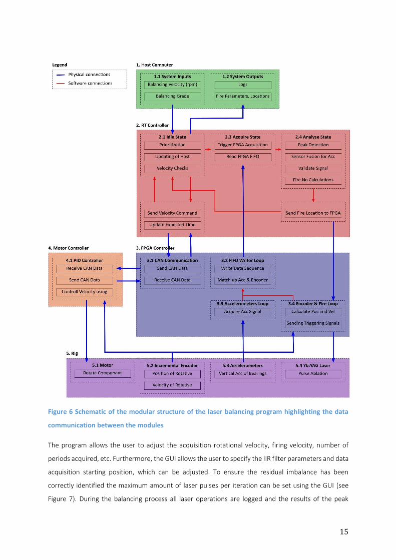
4.2 Design of the controller software The implementation of the methodology was realised by a combined 400 MHz real time (RT) processor

and a Spartan 3 field programmable gate array (FPGA) controller for the acquisition and evaluation of

the measurements; furthermore, for visualization of the process and logging, a personal computer was

connected. This three layer approach allows the system to use prioritisation to ensure that high priority

deterministic tasks, like data acquisition, are handled by the FPGA while lower priority non-

deterministic tasks, like logging and the updating of the GUI, are handled by the personal computer

operating system (see Figure 6).

A case structure was chosen as the program structure in order to keep the individual tasks modular.

Thus, each step, the acquisition, peak detection, triggering of the laser and calibration, was integrated

into the case structure on the RT as its own case. This approach ensures highest reliability and prevents

crashes during operation by allowing all code segments to run independently from each other,

however, it requires a careful optimized data communication structure.

Due to the limited computing resources, the amount of data collected needed to be minimized. The

encoder and accelerometer data is acquired at different frequencies in order to obey to the Nyquist

criteria [14] (i.e. the encoder is sampled at a significantly higher speed than the accelerometer).

Therefore, two different acquisition loops acquire data while the third matches the data at each

encoder pulse. Thus, only the acceleration data needs to be transferred to the RT since each data

sample represent one pulse change. This is an effective way of reducing data transfer and increasing

the system performance.

In order to ensure the accurate triggering of the laser at the detected imbalance position, the FPGA

continuously looks for laser firing commands from the RT and executes them if the encoder location

matches the one specified by the RT. An FPGA level velocity check prevents triggering during

acceleration and deceleration phases of the rotor. The trigger location is adjusted for the time delay

caused during the pulse built up within the fibre laser. The delay is obtained by empirical methods (i.e.

measurement using light sensitive paper) and converted into encoder steps, td, assuming a constant

radial velocity of the rotor bearing system as shown in Eq. ( 23 ).

θf = 2𝜋𝑟𝜔𝑡𝑑 ( 23 )

During the time of the material removal process, the FPGA ensures that the system runs at a constant

velocity; if it notices any disruptions the firing process is paused or stopped.

15

Figure 6 Schematic of the modular structure of the laser balancing program highlighting the data

communication between the modules

The program allows the user to adjust the acquisition rotational velocity, firing velocity, number of

periods acquired, etc. Furthermore, the GUI allows the user to specify the IIR filter parameters and data

acquisition starting position, which can be adjusted. To ensure the residual imbalance has been

correctly identified the maximum amount of laser pulses per iteration can be set using the GUI (see

Figure 7). During the balancing process all laser operations are logged and the results of the peak

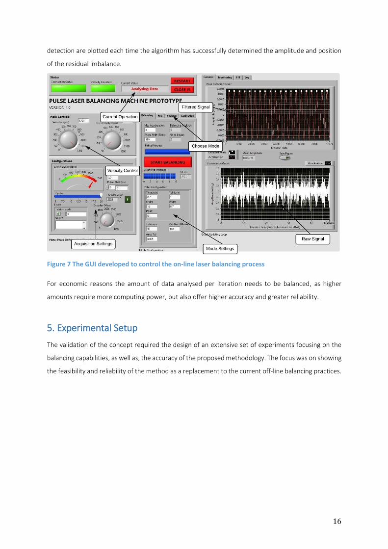
16

detection are plotted each time the algorithm has successfully determined the amplitude and position

of the residual imbalance.

Figure 7 The GUI developed to control the on-line laser balancing process

For economic reasons the amount of data analysed per iteration needs to be balanced, as higher

amounts require more computing power, but also offer higher accuracy and greater reliability.

5. Experimental Setup

The validation of the concept required the design of an extensive set of experiments focusing on the

balancing capabilities, as well as, the accuracy of the proposed methodology. The focus was on showing

the feasibility and reliability of the method as a replacement to the current off-line balancing practices.

17

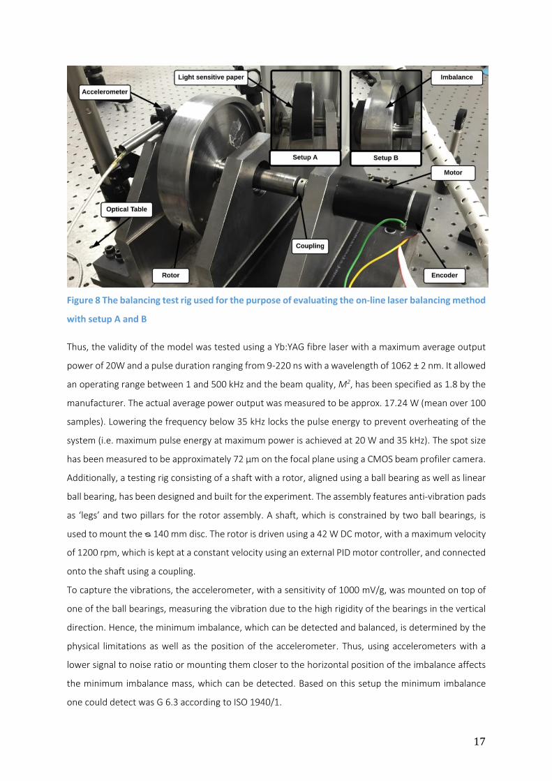
Figure 8 The balancing test rig used for the purpose of evaluating the on-line laser balancing method

with setup A and B

Thus, the validity of the model was tested using a Yb:YAG fibre laser with a maximum average output

power of 20W and a pulse duration ranging from 9-220 ns with a wavelength of 1062 ± 2 nm. It allowed

an operating range between 1 and 500 kHz and the beam quality, M2, has been specified as 1.8 by the

manufacturer. The actual average power output was measured to be approx. 17.24 W (mean over 100

samples). Lowering the frequency below 35 kHz locks the pulse energy to prevent overheating of the

system (i.e. maximum pulse energy at maximum power is achieved at 20 W and 35 kHz). The spot size

has been measured to be approximately 72 µm on the focal plane using a CMOS beam profiler camera.

Additionally, a testing rig consisting of a shaft with a rotor, aligned using a ball bearing as well as linear

ball bearing, has been designed and built for the experiment. The assembly features anti-vibration pads

as ‘legs’ and two pillars for the rotor assembly. A shaft, which is constrained by two ball bearings, is

used to mount the ᴓ 140 mm disc. The rotor is driven using a 42 W DC motor, with a maximum velocity

of 1200 rpm, which is kept at a constant velocity using an external PID motor controller, and connected

onto the shaft using a coupling.

To capture the vibrations, the accelerometer, with a sensitivity of 1000 mV/g, was mounted on top of

one of the ball bearings, measuring the vibration due to the high rigidity of the bearings in the vertical

direction. Hence, the minimum imbalance, which can be detected and balanced, is determined by the

physical limitations as well as the position of the accelerometer. Thus, using accelerometers with a

lower signal to noise ratio or mounting them closer to the horizontal position of the imbalance affects

the minimum imbalance mass, which can be detected. Based on this setup the minimum imbalance

one could detect was G 6.3 according to ISO 1940/1.

18

The accuracy of the system depends the correct pre-firing of the laser. Therefore, the first set of trials

focused on how accurately and precise the system can target the desired spot and ablated using PLA.

Therefore, light sensitive paper has been attached to the rotor (see Figure 8 Setup A) and after an initial

calibration shot to mark the desired position, 10 tracks of 8 pulses spaced approx. 1 mm apart have

been fired at 100, 400, 800, 1000 and 1200 rpm. Table 1 shows the parameters used for this trial; the

pre-trigging timing of 0.7 ms has been empirically determined for the system used, and varies

depending on the laser set-up. In order to evaluate the precision between individual run-ups, after

completion of the experiment, the system has been restarted and the same experiment has been re-

run in order to validate the precision of the pre-firing of the laser.

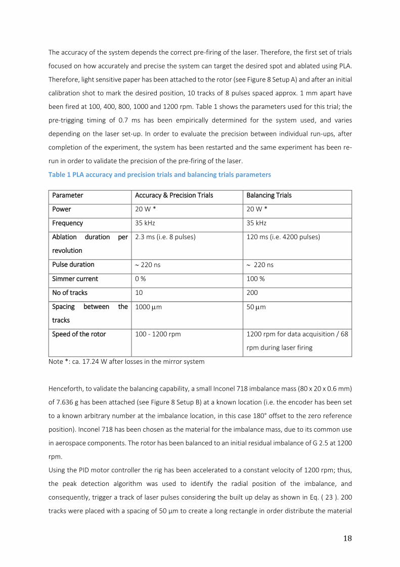
Table 1 PLA accuracy and precision trials and balancing trials parameters

Parameter Accuracy & Precision Trials Balancing Trials

Power 20 W * 20 W *

Frequency 35 kHz 35 kHz

Ablation duration per

revolution

2.3 ms (i.e. 8 pulses) 120 ms (i.e. 4200 pulses)

Pulse duration 220 ns 220 ns

Simmer current 0 % 100 %

No of tracks 10 200

Spacing between the

tracks

1000 m 50 m

Speed of the rotor 100 - 1200 rpm 1200 rpm for data acquisition / 68

rpm during laser firing

Note *: ca. 17.24 W after losses in the mirror system

Henceforth, to validate the balancing capability, a small Inconel 718 imbalance mass (80 x 20 x 0.6 mm)

of 7.636 g has been attached (see Figure 8 Setup B) at a known location (i.e. the encoder has been set

to a known arbitrary number at the imbalance location, in this case 180° offset to the zero reference

position). Inconel 718 has been chosen as the material for the imbalance mass, due to its common use

in aerospace components. The rotor has been balanced to an initial residual imbalance of G 2.5 at 1200

rpm.

Using the PID motor controller the rig has been accelerated to a constant velocity of 1200 rpm; thus,

the peak detection algorithm was used to identify the radial position of the imbalance, and

consequently, trigger a track of laser pulses considering the built up delay as shown in Eq. ( 23 ). 200

tracks were placed with a spacing of 50 µm to create a long rectangle in order distribute the material

19

removal over a large area and avoid the formation of a single “drilled hole”. Table 1 lists the relevant

parameters of the experiment.

The level of imbalance was evaluated according to ISO 1940/1 standard [17] using Equation ( 24 ),

which is the permissible specific unbalance, eper, multiplied by the radial velocity, .

𝐺 = 𝑒𝑝𝑒𝑟𝜔 ( 24 )

6. Model validation and discussion

The results were evaluated with a focus on the repeatability and reliability of the proposed method.

Initially, a feasibility study using a Simulink model has been conducted. Next, the accuracy and precision

trials of the chosen correctional method (i.e. pulse laser ablation), the above-introduced methodology

was used to balance a rotor with an added Inconel 718 sheet acting as the unbalance.

6.1 Evaluation of the accuracy and precision of the pulse laser ablation The system has been designed to ablate, accurately, mass at a given radial position. The method, in

order to quantify the accuracy and precision, it has been validated using light sensitive paper. As an

example these aspects of the system have been evaluated at five different radial velocities (100, 400,

800, 1000 and 1200 rpm) to allow covering a wide application ranges.

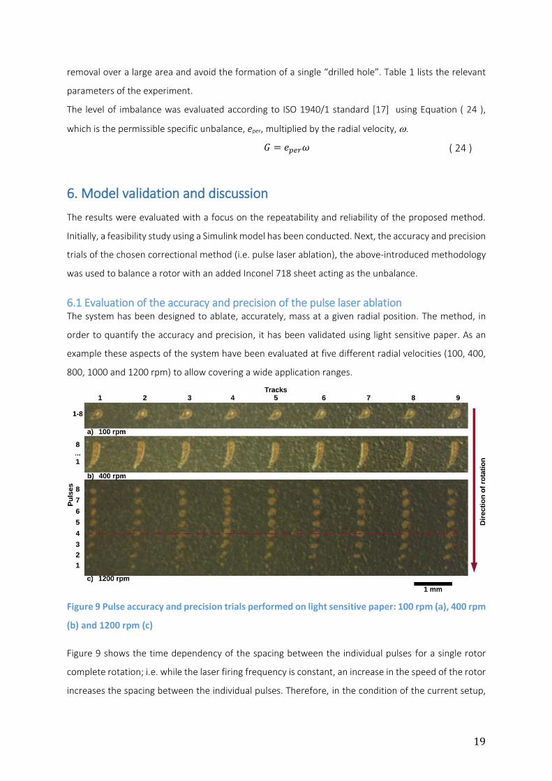
Figure 9 Pulse accuracy and precision trials performed on light sensitive paper: 100 rpm (a), 400 rpm

(b) and 1200 rpm (c)

Figure 9 shows the time dependency of the spacing between the individual pulses for a single rotor

complete rotation; i.e. while the laser firing frequency is constant, an increase in the speed of the rotor

increases the spacing between the individual pulses. Therefore, in the condition of the current setup,

20

to avoid drilling and instead ablate an area, speeds below 100 rpm are necessary for the laser firing

frequency chosen in this example (i.e. 35 kHz). As the pulse frequency approaches infinite (and the

pulse energy remains constant), higher rotational velocities of the part can be used, and therefore, the

process time can be minimized. Based on this rationale/example, an ablation velocity of 68 rpm has

been chosen for the rotor balancing in order to maximize material removal and avoid drilling. The pulses

of each track have been fired within one revolution using a static mirror system in the direction of

revolution (i.e. in this example 9 tracks require 9 revolutions – see Fig. 10). Hence, by comparing the

radial position of the ith pulse of all tracks the accuracy of the system is evaluated. In this example, 4th

pulse of the 1200 rpm example shows variations well below 50 µm (see red dotted reference line on

Figure 9 c)). Overall, at all velocities the pulses were very well aligned (error below 50 µm), thus proving

the accuracy in laser hitting the rotor in the same angular position that varies in max. 0.04 deg.

Additionally, in order to evaluate the repeatability of the system, after the initial nine tracks were fired

the rotor was stopped and externally disturbed (i.e. manually rotated), before it was again accelerated

to the desired velocity and the experiment was repeated. This replicates a scenario in real conditions

when an operator stops the system, examines the ablated surface and starts the system again. Hence,

each spot on the light sensitive paper has actually been created in two separate run-ups. Therefore, by

examining how closely the same position could have been hit again the repeatability of the system can

be evaluated; for example, Fig. 10c the individual spots were actually created by the 2 nearly perfectly

overlapped spots created in two runs with a stoppage and manual disturbance in between. Thus, in this

example, a repeatability error of less than 10 µm was achieved. Hence, the method was considered

very repeatable.

6.2 Balancing evaluation The system proved to be capable of balancing rotating components. The material removal amount is

highly dependent on the laser system used. Hence, depending on the purpose of the system (i.e. fine

balancing or general balancing) a different laser system would have to be used (i.e. in order to remove

masses of several grams a microsecond cutting laser would be suitable, while for fine balancing a

nanosecond engraving laser may suffice). As an example, the validation trials have been conducted with

the aim to reduce the unbalance of a rotor.

Initial measurements (see Table 2) detected the imbalance at 195° (the imbalance has been attached

at the reference position of 180°). However, this includes the phase shift, as the acceleration cannot be

measured directly at the rotor. In this case, the vibration is measured on top of the right bearing, which

caused a phase shift of 15°. Hence, the program determined the laser triggering position to be 179.71°

accounting for the 15° phase shift and a trigger time delay of the system of 0.7 ms for a rotational speed

of 68. The balancing grade was determined to be G 22.5 at 1200 rpm.

21

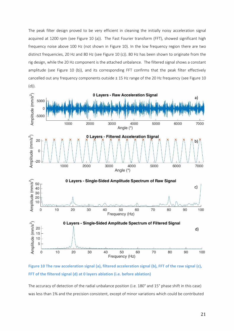
The peak filter design proved to be very efficient in cleaning the initially noisy acceleration signal

acquired at 1200 rpm (see Figure 10 (a)). The Fast Fourier transform (FFT), showed significant high

frequency noise above 100 Hz (not shown in Figure 10). In the low frequency region there are two

distinct frequencies, 20 Hz and 80 Hz (see Figure 10 (c)). 80 Hz has been shown to originate from the

rig design, while the 20 Hz component is the attached unbalance. The filtered signal shows a constant

amplitude (see Figure 10 (b)), and its corresponding FFT confirms that the peak filter effectively

cancelled out any frequency components outside ± 15 Hz range of the 20 Hz frequency (see Figure 10

(d)).

Figure 10 The raw acceleration signal (a), filtered acceleration signal (b), FFT of the raw signal (c),

FFT of the filtered signal (d) at 0 layers ablation (i.e. before ablation)

The accuracy of detection of the radial unbalance position (i.e. 180° and 15° phase shift in this case)

was less than 1% and the precision consistent, except of minor variations which could be contributed

a)

b)

d)

c)

22

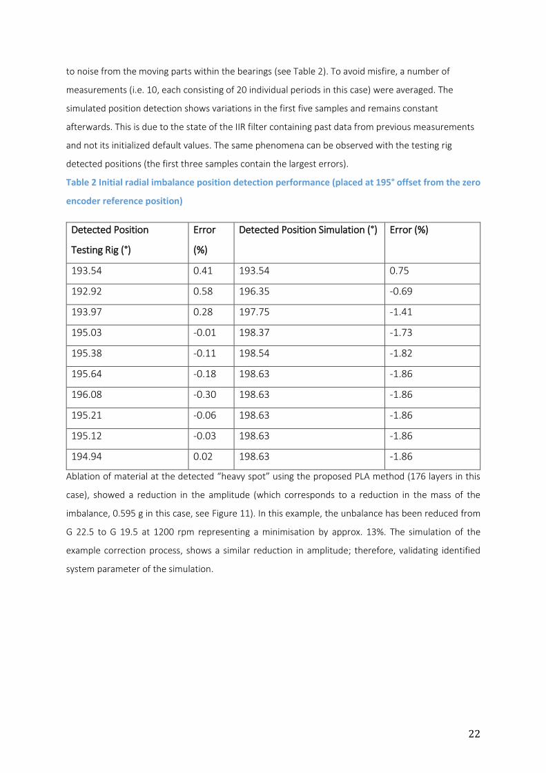
to noise from the moving parts within the bearings (see Table 2). To avoid misfire, a number of

measurements (i.e. 10, each consisting of 20 individual periods in this case) were averaged. The

simulated position detection shows variations in the first five samples and remains constant

afterwards. This is due to the state of the IIR filter containing past data from previous measurements

and not its initialized default values. The same phenomena can be observed with the testing rig

detected positions (the first three samples contain the largest errors).

Table 2 Initial radial imbalance position detection performance (placed at 195° offset from the zero

encoder reference position)

Detected Position

Testing Rig (°)

Error

(%)

Detected Position Simulation (°) Error (%)

193.54 0.41 193.54 0.75

192.92 0.58 196.35 -0.69

193.97 0.28 197.75 -1.41

195.03 -0.01 198.37 -1.73

195.38 -0.11 198.54 -1.82

195.64 -0.18 198.63 -1.86

196.08 -0.30 198.63 -1.86

195.21 -0.06 198.63 -1.86

195.12 -0.03 198.63 -1.86

194.94 0.02 198.63 -1.86

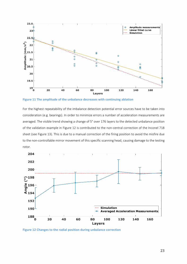
Ablation of material at the detected “heavy spot” using the proposed PLA method (176 layers in this

case), showed a reduction in the amplitude (which corresponds to a reduction in the mass of the

imbalance, 0.595 g in this case, see Figure 11). In this example, the unbalance has been reduced from

G 22.5 to G 19.5 at 1200 rpm representing a minimisation by approx. 13%. The simulation of the

example correction process, shows a similar reduction in amplitude; therefore, validating identified

system parameter of the simulation.

23

Figure 11 The amplitude of the unbalance decreases with continuing ablation

For the highest repeatability of the imbalance detection potential error sources have to be taken into

consideration (e.g. bearings). In order to minimize errors a number of acceleration measurements are

averaged. The visible trend showing a change of 5° over 176 layers to the detected unbalance position

of the validation example in Figure 12 is contributed to the non-central correction of the Inconel 718

sheet (see Figure 13). This is due to a manual correction of the firing position to avoid the misfire due

to the non-controllable mirror movement of this specific scanning head, causing damage to the testing

rotor.

Figure 12 Changes to the radial position during unbalance correction

24

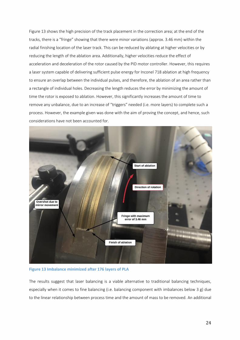
Figure 13 shows the high precision of the track placement in the correction area; at the end of the

tracks, there is a “fringe” showing that there were minor variations (approx. 3.46 mm) within the

radial finishing location of the laser track. This can be reduced by ablating at higher velocities or by

reducing the length of the ablation area. Additionally, higher velocities reduce the effect of

acceleration and deceleration of the rotor caused by the PID motor controller. However, this requires

a laser system capable of delivering sufficient pulse energy for Inconel 718 ablation at high frequency

to ensure an overlap between the individual pulses, and therefore, the ablation of an area rather than

a rectangle of individual holes. Decreasing the length reduces the error by minimizing the amount of

time the rotor is exposed to ablation. However, this significantly increases the amount of time to

remove any unbalance, due to an increase of “triggers” needed (i.e. more layers) to complete such a

process. However, the example given was done with the aim of proving the concept, and hence, such

considerations have not been accounted for.

Figure 13 Imbalance minimized after 176 layers of PLA

The results suggest that laser balancing is a viable alternative to traditional balancing techniques,

especially when it comes to fine balancing (i.e. balancing component with imbalances below 3 g) due

to the linear relationship between process time and the amount of mass to be removed. An additional

25

study conducted for Rolls-Royce plc. suggests that the time to remove 1 g could be reduced to as little

as ≈ 7 mins enabling wider application of the proposed method.

7. Conclusion

Balancing has become a standard process in many industries including the automotive, medical,

defence and power turbine industry. Henceforth, most recent research improves on the traditional

balancing methods without changing the two-step nature of the process, i.e. the identification of the

imbalance location and mass, and then the removal of such by a separate machine. Due to space

requirements for such a machine, in-situ applications are usually not possible. Lasers, however, allow

machining in space restricted environments. This paper reports on a model to enable in-situ online

pulsed laser balancing.

A model for on-the-fly PLA balancing has been developed, consisting of a state space model

of the rig. The model has shown to be able to predict accurately (less than 5% error) the

impact of pulse laser balancing onto the rotor. It is used as both a feasibility study as well as a

guide to evaluate the effectiveness of pulse laser balancing.

The method has been integrated into a specifically developed system. An adaptable IIR peak

filter has been designed to filter acceleration signals recorded at varying rotational velocities.

The peak filter has been designed in order to minimize false positives and rejected

measurements. It automatically adapts to the measurements and does not require any user

interactions. It has shown to be able to detect imbalances with an accuracy of less than 1%.

The system has been developed to be accurate and repeatable, by considering time delays

and velocity variations over a wide range over rotational speeds (100 – 1200 rpm). This has

been achieved by using a FPGA to evaluate the velocity and position of the rotor, as well as

trigger the laser within the same loop. The systems accuracy has been shown to be below 50

µm and its repeatability below 30 µm.

The balancing capabilities of the system have been demonstrated by removing a small

amount of Inconel 718 as an example (approx. 0.5 g), and henceforth, reducing the overall

unbalance of the rotor. The use of different laser systems in order to remove larger quantities

in a reduced timespan have been discussed. It has been concluded that the method is viable

on an industrial scale due to cost savings in the long-term by not requiring skilled labor as well

as the potential in-situ applications.

Hence, the proposed balancing method allows the users to save time and cost by removing the

two-step nature of traditional balancing. Furthermore, the reliance on manual skilled labour can be

further decreased. Further research in the effects of different laser systems for different balancing

26

application is needed; nevertheless, laser balancing offers a solid solution to balancing on an

industrial scale.

Acknowledgements

The author would like to acknowledge the generous support of Rolls-Royce plc. and especially to Mr.

Peter Winton and Mr. Mike Harrison as well as the EPSRC for the CASE award scholarship.

Special thanks go to Salvador Cobos Guzman for his assistance and advice during the project.

References

[1] R. B. McMillian, Rotating Machinery: Practical Solutions to Unbalance and Misalignment.

Fairmont Press, 2003.

[2] Schenck, “Schenck USA - 100 years of balancing technology,” 2014. [Online]. Available:

http://www.schenck-usa.com/company/information/history.php. [Accessed: 01-Sep-2014].

[3] C. F. Coombs, “Printed Circuits Handbook (McGraw Hill Handbooks): Amazon.co.uk: Clyde F.

Coombs: Books,” 2007. [Online]. Available: http://www.amazon.co.uk/Printed-Circuits-

Handbook-McGraw-Handbooks/dp/0071467343. [Accessed: 01-Sep-2014].

[4] C. Kim and C. Lee, “In situ runout identification in active magnetic bearing system by

extended influence coefficient method,” IEEE/ASME Trans. Mechatronics, 1997.

[5] R. S. Demuth, R. A. Rio, and D. P. Fleming, “Laser balancing demonstration on a high-speed

flexible rotor,” 1979.

[6] P. Schultz, “Dynamisches Auswuchten von rotierenden Körpern während des Laufes mit Hilfe

des Lasers,” VDI-Zeitung, Hamburg, pp. 136–140, 1969.

[7] S. Davies, J. Kell, M. . Kong, D. Axinte, and K. Perkins, “ICALEO 2011 Paper #M505 (Laser

Ablation: Optimising Material Removal Rate with Limited Oxidation for Ti6Al4V) - LIA,”

ICALEO 2011, 2011. [Online]. Available: https://www.lia.org/store//ICA11_M505. [Accessed:

15-Sep-2014].

[8] S. Davies, J. Kell, M. . Kong, D. Axinte, and K. Perkins, “Laser Ablation: Optimising Material

Removal Rate with limited Oxidation of TI6A14V,” pp. 906–913.

[9] J. Figueira and S. Thomas, “Damage thresholds at metal surfaces for short pulse IR lasers,”

IEEE J. Quantum Electron., vol. 18, no. 9, pp. 1381–1386, Sep. 1982.

[10] J. F. Walton, M. Cronin, and R. Mehta, “Advanced balancing using laser machining,” SAE,

Aerosp. Technol. Conf. Expo., vol. -1, Sep. 1991.

[11] R. Tiwari and V. Chakravarthy, “Simultaneous estimation of the residual unbalance and

bearing dynamic parameters from the experimental data in a rotor-bearing system,” Mech.

Mach. Theory, vol. 44, no. 4, pp. 792–812, Apr. 2009.

27

[12] W.-S. Gan and S. M. Kuo, Embedded Signal Processing with the Micro Signal Architecture.

John Wiley & Sons, 2007.

[13] R. G. Lyons, Understanding Digital Signal Processing, vol. 1. Pearson Education, 2010.

[14] U. Grenander, Probability and Statistics: The Harald Cramér Volume. Alqvist & Wiksell, 1959.

[15] A. Hasçalık and M. Ay, “CO2 laser cut quality of Inconel 718 nickel – based superalloy,” Opt.

Laser Technol., vol. 48, pp. 554–564, Jun. 2013.

[16] W.-T. Chien and S.-C. Hou, “Investigating the recast layer formed during the laser trepan

drilling of Inconel 718 using the Taguchi method,” Int. J. Adv. Manuf. Technol., vol. 33, no. 3–

4, pp. 308–316, Apr. 2006.

[17] International Organization for Standardization, “ISO 1940-1 Mechanical vibration — Balance

quality requirements for rotors in a constant (rigid) state —,” 2003.

Appendix

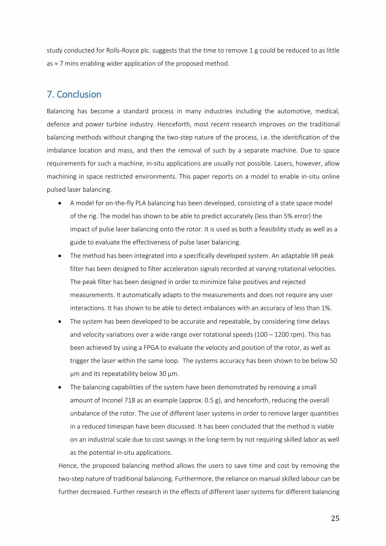
The A, B, C and D are the state, input, output and feedthrough matrices given as

𝐴 =

[

0 0 0 0 1 0 0 00 0 0 0 0 1 0 00 0 0 0 0 0 1 00 0 0 0 0 0 0 1

𝑘1𝑥𝑥𝑏1 𝑘1𝑥𝑦𝑏1 𝑘2𝑥𝑥𝑏2 𝑘2𝑥𝑦𝑏2 𝑐1𝑥𝑥𝑏1 𝑐1𝑥𝑦𝑏7 𝑐2𝑥𝑥𝑏2 𝑐2𝑥𝑦𝑏9

𝑘1𝑦𝑥𝑏1 𝑘1𝑦𝑦𝑏1 𝑘2𝑦𝑥𝑏2 𝑘2𝑦𝑥𝑏2 𝑐1𝑦𝑥𝑏7 𝑐1𝑦𝑦𝑏1 𝑐2𝑦𝑥𝑏9 𝑐2𝑦𝑦𝑏2

𝑘1𝑥𝑥𝑏2 𝑘1𝑥𝑦𝑏2 𝑘2𝑥𝑥𝑏3 𝑘2𝑥𝑦𝑏3 𝑐1𝑥𝑥𝑏2 𝑐1𝑥𝑦𝑏8 𝑐2𝑥𝑥𝑏3 𝑐2𝑥𝑦𝑏10

𝑘1𝑦𝑥𝑏2 𝑘1𝑦𝑦𝑏2 𝑘2𝑦𝑥𝑏3 𝑘2𝑦𝑦𝑏3 𝑐1𝑦𝑥𝑏8 𝑐1𝑦𝑦𝑏2 𝑐2𝑦𝑥𝑏10 𝑐2𝑦𝑦𝑏3 ]

(1)

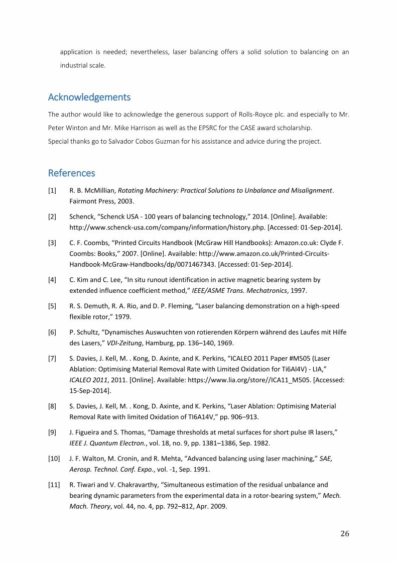
𝐵 =

[

0 00 00 00 0

𝑏6(𝑙12𝑧1 − 𝑙1𝑙2𝑧2) 0

0 𝑏6(𝑙22𝑧1 − 𝑙1𝑙2𝑧2)

𝑏6(𝑙12𝑧2 − 𝑙1𝑙2𝑧1) 0

0 𝑏6(𝑙22𝑧2 − 𝑙1𝑙2𝑧1)]

(2)

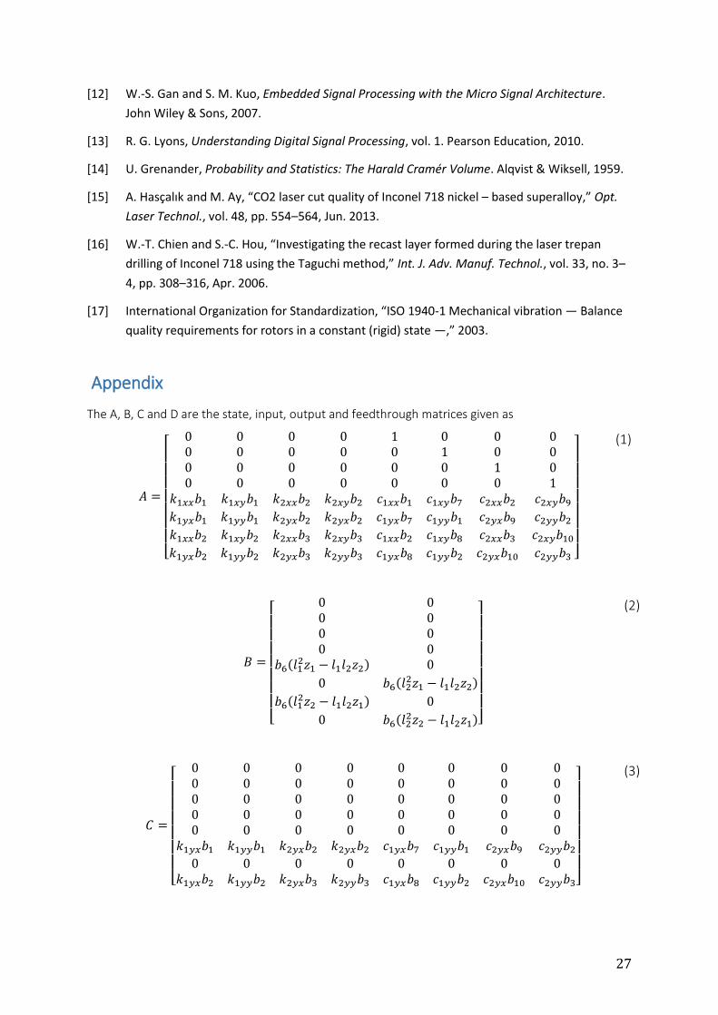
𝐶 =

[

0 0 0 0 0 0 0 00 0 0 0 0 0 0 00 0 0 0 0 0 0 00 0 0 0 0 0 0 00 0 0 0 0 0 0 0

𝑘1𝑦𝑥𝑏1 𝑘1𝑦𝑦𝑏1 𝑘2𝑦𝑥𝑏2 𝑘2𝑦𝑥𝑏2 𝑐1𝑦𝑥𝑏7 𝑐1𝑦𝑦𝑏1 𝑐2𝑦𝑥𝑏9 𝑐2𝑦𝑦𝑏2

0 0 0 0 0 0 0 0𝑘1𝑦𝑥𝑏2 𝑘1𝑦𝑦𝑏2 𝑘2𝑦𝑥𝑏3 𝑘2𝑦𝑦𝑏3 𝑐1𝑦𝑥𝑏8 𝑐1𝑦𝑦𝑏2 𝑐2𝑦𝑥𝑏10 𝑐2𝑦𝑦𝑏3]

(3)

28

𝐷 =

[ 0 00 00 00 00 00 𝑏6(𝑙2

2𝑧1 − 𝑙1𝑙2𝑧2)0 00 𝑏6(𝑙2

2𝑧2 − 𝑙1𝑙2𝑧1)]

(4)

where

𝑏1 = −

(𝑚𝑙12 + 𝑖𝑡)

𝑚𝑖𝑡(𝑙1 + 𝑙2)2, 𝑏2 =

(𝑚𝑙1𝑙2 − 𝑖𝑡)

𝑚𝑖𝑡(𝑙1 + 𝑙2)2

𝑏3 = −

(𝑚𝑙22 + 𝑖𝑡)

𝑚𝑖𝑡(𝑙1 + 𝑙2)2, 𝑏4 =

𝑖𝑝(𝑚𝜔𝑙12 + 𝑚𝜔𝑙1𝑙2)

𝑚𝑖𝑡(𝑙1 + 𝑙2)2

𝑏5 =

𝑖𝑝(𝑚𝜔𝑙22 + 𝑚𝜔𝑙1𝑙2)

𝑚𝑖𝑡(𝑙1 + 𝑙2)2

, 𝑏6 =𝜔2𝑖𝑡(𝑧1 + 𝑧2) + 𝑚𝜔2

𝑚𝑖𝑡(𝑙1 + 𝑙2)2

𝑏7 = 𝑏1 + 𝑏4, 𝑏8 = 𝑏2 + 𝑏5

𝑏9 = 𝑏2 + 𝑏4, 𝑏10 = 𝑏3 + 𝑏5