PubTeX output 1999.11.16:1337 - CSASS courses/ProcCorr.pdf · 273 CHAPTER12 The CORR Procedure Overview 273 Procedure Syntax 277 PROC CORR Statement 278 BY Statement 283 FREQ …

273

C H A P T E R

12The CORR Procedure

Overview 273Procedure Syntax 277

PROC CORR Statement 278

BY Statement 283

FREQ Statement 283

PARTIAL Statement 284VAR Statement 284

WEIGHT Statement 285

WITH Statement 286

Concepts 286

Interpreting Correlation Coefficients 286

Determining Computer Resources 287Statistical Computations 289

Pearson Product-Moment Correlation 289

Spearman Rank-Order Correlation 290

Kendall’s tau-b 290

Hoeffding’s Measure of Dependence, D 291Partial Correlation 291

Cronbach’s Coefficient Alpha 293

Probability Values 295

Results 297

Missing Values 297Procedure Output 297

Output Data Sets 298

Examples 300

Example 1: Computing Pearson Correlations and Other Measures of Association 300

Example 2: Computing Rectangular Correlation Statistics with Missing Data 303

Example 3: Computing Cronbach’s Coefficient Alpha 306Example 4: Storing Partial Correlations in an Output Data Set 309

References 312

Overview

The CORR procedure is a statistical procedure for numeric random variables thatcomputes Pearson correlation coefficients, three nonparametric measures of association,and the probabilities associated with these statistics. The correlation statistics include

� Pearson product-moment and weighted product-moment correlation

� Spearman rank-order correlation

� Kendall’s tau-b

274 Overview 4 Chapter 12

� Hoeffding’s measure of dependence, D� Pearson, Spearman, and Kendall partial correlation.

PROC CORR also computes Cronbach’s coefficient alpha for estimating reliability.The default correlation analysis includes descriptive statistics, Pearson correlation

statistics, and probabilities for each analysis variable. You can save the correlationstatistics in a SAS data set for use with other statistical and reporting procedures.

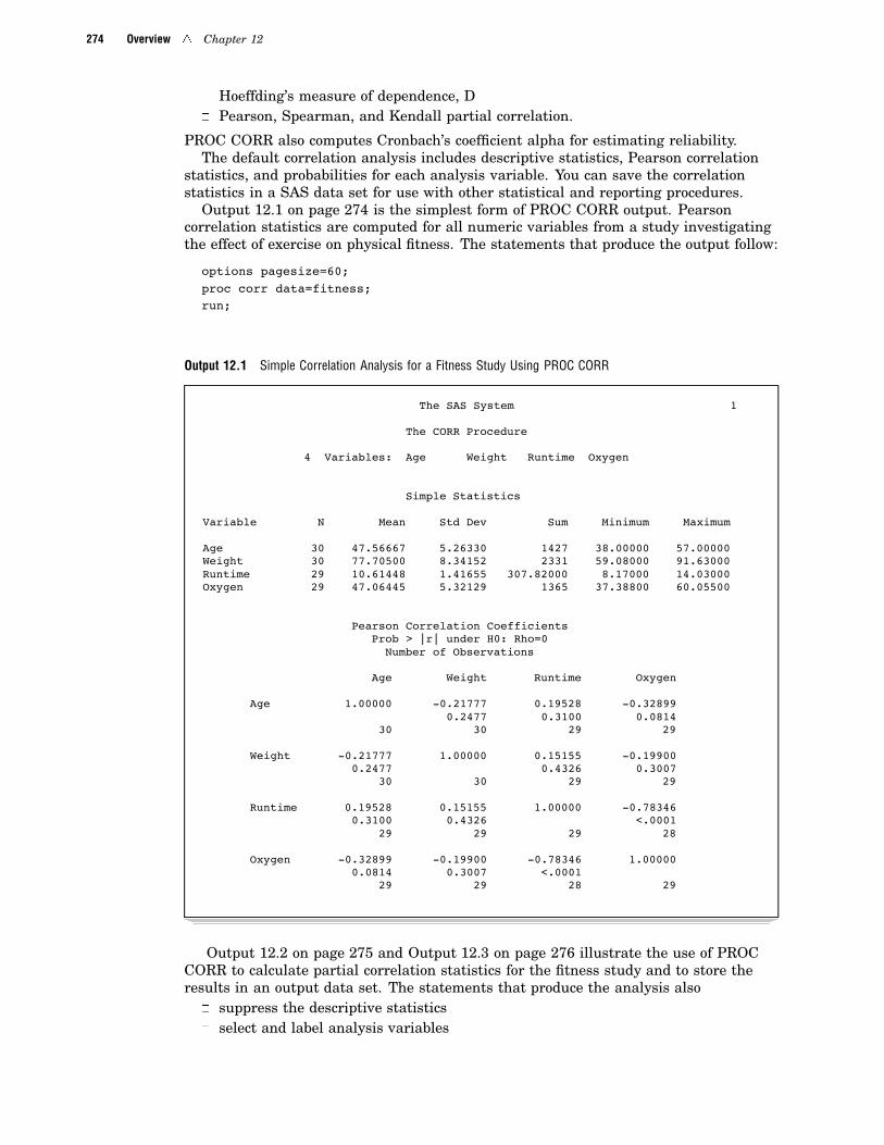
Output 12.1 on page 274 is the simplest form of PROC CORR output. Pearsoncorrelation statistics are computed for all numeric variables from a study investigatingthe effect of exercise on physical fitness. The statements that produce the output follow:

options pagesize=60;proc corr data=fitness;run;

Output 12.1 Simple Correlation Analysis for a Fitness Study Using PROC CORR

The SAS System 1

The CORR Procedure

4 Variables: Age Weight Runtime Oxygen

Simple Statistics

Variable N Mean Std Dev Sum Minimum Maximum

Age 30 47.56667 5.26330 1427 38.00000 57.00000Weight 30 77.70500 8.34152 2331 59.08000 91.63000Runtime 29 10.61448 1.41655 307.82000 8.17000 14.03000Oxygen 29 47.06445 5.32129 1365 37.38800 60.05500

Pearson Correlation CoefficientsProb > |r| under H0: Rho=0

Number of Observations

Age Weight Runtime Oxygen

Age 1.00000 -0.21777 0.19528 -0.328990.2477 0.3100 0.0814

30 30 29 29

Weight -0.21777 1.00000 0.15155 -0.199000.2477 0.4326 0.3007

30 30 29 29

Runtime 0.19528 0.15155 1.00000 -0.783460.3100 0.4326 <.0001

29 29 29 28

Oxygen -0.32899 -0.19900 -0.78346 1.000000.0814 0.3007 <.0001

29 29 28 29

Output 12.2 on page 275 and Output 12.3 on page 276 illustrate the use of PROCCORR to calculate partial correlation statistics for the fitness study and to store theresults in an output data set. The statements that produce the analysis also

� suppress the descriptive statistics� select and label analysis variables

The CORR Procedure 4 Overview 275

� exclude all observations with missing values� calculate the partial covariance matrix� calculate three types of partial correlation coefficients� generate an output data set that contains Pearson correlation statistics and print

the output data set.

For an explanation of the program that produces the following output, see Example 4on page 309.

276 Overview 4 Chapter 12

Output 12.2 Customized Correlation Analysis with Partial Covariances and Correlation Statistics

Partial Correlations for a Fitness and Exercise Study 1

The CORR Procedure

1 Partial Variables: Age

3 Variables: Weight Oxygen Runtime

Partial Covariance Matrix, DF = 26

Weight Oxygen Runtime

Weight Wt in kg 72.43742055 -12.75113194 2.06766763

Oxygen O2 use -12.75113194 27.01654904 -5.59370556

Runtime 1.5 mi in minutes 2.06766763 -5.59370556 1.94512451

Pearson Partial Correlation Coefficients, N = 28

Prob > |r| under H0: Partial Rho=0


Weight 1.00000 -0.28824 0.17419

Wt in kg 0.1448 0.3849

Oxygen -0.28824 1.00000 -0.77163

O2 use 0.1448 <.0001

Runtime 0.17419 -0.77163 1.00000

1.5 mi in minutes 0.3849 <.0001

Spearman Partial Correlation Coefficients, N = 28



Weight 1.00000 -0.16407 0.08708

Wt in kg 0.4135 0.6658

Oxygen -0.16407 1.00000 -0.67112

O2 use 0.4135 0.0001

Runtime 0.08708 -0.67112 1.00000

1.5 mi in minutes 0.6658 0.0001

Kendall Partial Tau b Correlation Coefficients, N = 28


Weight 1.00000 -0.09021 0.02854

Wt in kg

Oxygen -0.09021 1.00000 -0.52158

O2 use

Runtime 0.02854 -0.52158 1.00000

1.5 mi in minutes

The CORR Procedure 4 Procedure Syntax 277

Output 12.3 Output Data Set with Pearson Partial Correlation Statistics

Pearson Correlation Statistics Using the PARTIAL Statement 2Output Data Set from PROC CORR

_TYPE_ _NAME_ Weight Oxygen Runtime

COV Weight 72.4374 -12.7511 2.0677COV Oxygen -12.7511 27.0165 -5.5937COV Runtime 2.0677 -5.5937 1.9451MEAN 0.0000 0.0000 0.0000STD 8.5110 5.1977 1.3947N 28.0000 28.0000 28.0000CORR Weight 1.0000 -0.2882 0.1742CORR Oxygen -0.2882 1.0000 -0.7716CORR Runtime 0.1742 -0.7716 1.0000

Procedure SyntaxTip: Supports the Output Delivery System, see “Output Delivery System” on page 19Reminder: You can use the ATTRIB, FORMAT, LABEL, and WHERE statements. SeeChapter 3, "Statements with the Same Function in Multiple Procedures," for details.You can also use any global statements as well. See Chapter 2, "Fundamental Conceptsfor Using Base SAS Procedures," for a list.

PROC CORR <option(s)>;BY <DESCENDING> variable-1<…<DESCENDING> variable-n>

<NOTSORTED>;FREQ frequency-variable;PARTIAL variable(s);VAR variable(s);WEIGHT weight-variable;WITH variable(s);

To do this Use this statement

Produce separate correlation analyses for each BY group BY

Identify a variable whose values represent the frequency of eachobservation

FREQ

Identify controlling variables to compute Pearson, Spearman, orKendall partial correlation coefficients

PARTIAL

Identify variables to correlate and their order in the correlationmatrix

VAR

278 PROC CORR Statement 4 Chapter 12

To do this Use this statement

Identify a variable whose values weight each observation to computePearson weight product-moment correlation

WEIGHT

Compute correlations for specific combinations of variables WITH

PROC CORR Statement

PROC CORR <option(s)>;

To do this Use this option

Specify the input data set DATA=

Create output data sets

Specify an output data set to contain Hoeffding’s D statistics OUTH=

Specify an output data set to contain Kendall correlations OUTK=

Specify an output data set to contain Pearson correlations OUTP=

Specify an output data set to contain Spearman correlations OUTS=

Control statistical analysis

Exclude observations with nonpositive weight values from theanalysis

EXCLNPWGT

Request Hoeffding’s measure of dependence, D HOEFFDING

Request Kendall’s tau-b KENDALL

Request Pearson product-moment correlation PEARSON

Request Spearman rank-order correlation SPEARMAN

Control Pearson correlation statistics

Compute Cronbach’s coefficient alpha ALPHA

Compute covariances COV

Compute corrected sums of squares and crossproducts CSSCP

Exclude missing values NOMISS

Specify singularity criterion SINGULAR=

Compute sums of squares and crossproducts SSCP

Specify the divisor for variance calculations VARDEF=

Control printed output

Specify the number and order of correlation coefficients BEST=

Suppress Pearson correlations NOCORR

Suppress all printed output NOPRINT

Suppress significance probabilities NOPROB

The CORR Procedure 4 PROC CORR Statement 279

To do this Use this option

Suppress descriptive statistics NOSIMPLE

Change the order of correlation coefficients RANK

Options

ALPHAcalculates and prints Cronbach’s coefficient alpha. PROC CORR computes separatecoefficients using raw and standardized values (scaling the variables to a unitvariance of 1). For each VAR statement variable, PROC CORR computes thecorrelation between the variable and the total of the remaining variables. It alsocomputes Cronbach’s coefficient alpha using only the remaining variables.Main discussion: “Cronbach’s Coefficient Alpha” on page 293Restriction: If you use a WITH statement, ALPHA is invalid.Interaction: ALPHA invokes PEARSON.Interaction: If you specify OUTP=, the output data set also contains six

observations with Cronbach’s coefficient alpha.Interaction: When you use the PARTIAL statement, PROC CORR calculates

Cronbach’s coefficient alpha for partialled variables.See also: OUTP= optionFeatured in: Example 3 on page 306

BEST=nprints n correlation coefficients for each variable. Correlations are ordered fromhighest to lowest in absolute value. Otherwise, PROC CORR prints correlations in arectangular table using the variable names as row and column labels.Interaction: When you specify HOEFFDING, PROC CORR prints the D statistics

in order from highest to lowest.Range: 1 to the maximum number of variables

COVcalculates and prints covariances.Interaction: COV invokes PEARSON.Interaction: If you specify OUTP=, the output data set contains the covariance

matrix and the _TYPE_ variable value is COV.Interaction: When you use the PARTIAL statement, PROC CORR computes a

partial covariance matrix.See also: OUTP= optionFeatured in: Example 2 on page 303 and Example 4 on page 309

CSSCPprints the corrected sums of squares and crossproducts.Interaction: CSSCP invokes PEARSON.Interaction: If you specify OUTP=, the output data set contains a CSSCP matrix

and the _TYPE_ variable value is CSSCP. If you use a PARTIAL statement, theoutput data set contains a partial CSSCP matrix.

Interaction: When you use a PARTIAL statement, PROC CORR prints both anunpartial and a partial CSSCP matrix.

See also: OUTP= option


DATA=SAS-data-setspecifies the input SAS data set.Main discussion: “Input Data Sets” on page 18

EXCLNPWGTexcludes observations with nonpositive weight values (zero or negative) from theanalysis. By default, PROC CORR treats observations with negative weights likethose with zero weights and counts them in the total number of observations.Requirement: You must use a WEIGHT statement.See also: “WEIGHT Statement” on page 285

HOEFFDINGcalculates and prints Hoeffding’s D statistics. This D statistic is 30 times larger thanthe usual definition and scales the range between -0.5 and 1 so that only largepositive values indicate dependence.Main discussion: “Hoeffding’s Measure of Dependence, D” on page 291Restriction: When you use a WEIGHT or PARTIAL statement, HOEFFDING is

invalid.Featured in: Example 1 on page 300

KENDALLcalculates and prints Kendall tau-b coefficients based on the number of concordantand discordant pairs of observations. Kendall’s tau-b ranges from -1 to 1.Main discussion: “Kendall’s tau-b” on page 290Restriction: When you use a WEIGHT statement, KENDALL is invalid.Interactions: When you use a PARTIAL statement, probability values for Kendall’s

partial tau-b are not available.Featured in: Example 4 on page 309

NOCORRsuppresses calculating and printing of Pearson correlations.Interaction: If you specify OUTP=, the data set type remains CORR. To change the

data set type to COV, CSSCP, or SSCP, use the TYPE= data set option.See also: “Output Data Sets” on page 298Featured in: Example 3 on page 306

NOMISSexcludes observations with missing values from the analysis. Otherwise, PROCCORR computes correlation statistics using all the nonmissing pairs of variables.Main discussion: “Missing Values” on page 297Tip: Using NOMISS is computationally more efficient.Featured in: Example 3 on page 306

NOPRINTsuppresses all printed output.Tip: Use NOPRINT when you want to create an output data set only.

NOPROBsuppresses printing the probabilities associated with each correlation coefficient.

NOSIMPLEsuppresses printing simple descriptive statistics for each variable. However, if yourequest an output data set, the output data set still contains simple descriptivestatistics for the variables.Featured in: Example 2 on page 303

The CORR Procedure 4 PROC CORR Statement 281

OUTH=output-data-setcreates an output data set containing Hoeffding’s D statistics. The contents of theoutput data set are similar to the OUTP= data set.Main discussion: “Output Data Sets” on page 298Interaction: OUTH= invokes HOEFFDING.

OUTK=output-data-setcreates an output data set containing Kendall correlation statistics. The contents ofthe output data set are similar to the OUTP= data set.Main discussion: “Output Data Sets” on page 298Interaction: OUTK= option invokes KENDALL.

OUTP=output-data-setcreates an output data set containing Pearson correlation statistics. This data setalso includes means, standard deviations, and the number of observations. The valueof the _TYPE_ variable is CORR.Main discussion: “Output Data Sets” on page 298Interaction: OUTP= invokes PEARSON.Interaction: If you specify ALPHA, the output data set also contains six

observations with Cronbach’s coefficient alpha.Featured in: Example 4 on page 309

OUTS=SAS-data-setcreates an output data set containing Spearman correlation statistics. The contentsof the output data set are similar to the OUTP= data set.Main discussion: “Output Data Sets” on page 298Interaction: OUTS= invokes SPEARMAN.

PEARSONcalculates and prints Pearson product-moment correlations when you use theHOEFFDING, KENDALL, or SPEARMAN option. If you omit the correlation type,PROC CORR automatically produces Pearson correlations. The correlations rangefrom -1 to 1.Main discussion: “Pearson Product-Moment Correlation” on page 289Featured in: Example 1 on page 300

RANKprints the correlation coefficients for each variable. Correlations are ordered fromhighest to lowest in absolute value. Otherwise, PROC CORR prints correlations in arectangular table using the variable names as row and column labels.Interaction: If you use HOEFFDING, PROC CORR prints the D statistics in order

from highest to lowest.

SINGULAR=pspecifies the criterion for determining the singularity of a variable when you use aPARTIAL statement. A variable is considered singular if its corresponding diagonalelement after Cholesky decomposition has a value less than p times the originalunpartialled corrected sum of squares of that variable.Main discussion: “Partial Correlation” on page 291Default: 1E-8Range: between 0 and 1

SPEARMANcalculates and prints Spearman correlation coefficients based on the ranks of thevariables. The correlations range from -1 to 1.


Main discussion: “Spearman Rank-Order Correlation” on page 290Restriction: When you specify a WEIGHT statement, SPEARMAN is invalid.

Example 1 on page 300Featured in:

SSCPprints the sums of squares and crossproducts.Interaction: SSCP invokes PEARSON.Interaction: When you specify OUTP=, the output data set contains a SSCP matrix

and the _TYPE_ variable value is SSCP. If you use a PARTIAL statement, theoutput data set does not contain an SSCP matrix.

Interaction: When you use a PARTIAL statement, PROC CORR prints theunpartial SSCP matrix.

Featured in: Example 2 on page 303

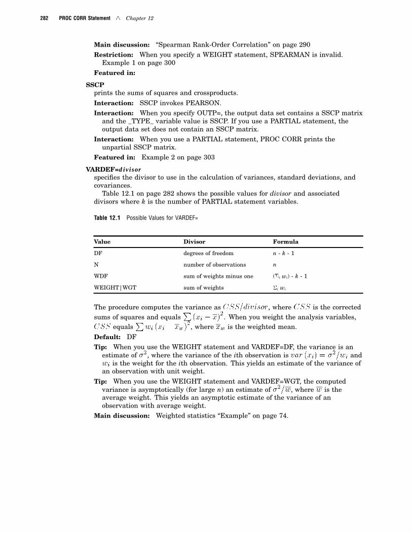
VARDEF=divisorspecifies the divisor to use in the calculation of variances, standard deviations, andcovariances.

Table 12.1 on page 282 shows the possible values for divisor and associateddivisors where k is the number of PARTIAL statement variables.

Table 12.1 Possible Values for VARDEF=

Value Divisor Formula

DF degrees of freedom n - k - 1

N number of observations n

WDF sum of weights minus one (�i wi) - k - 1

WEIGHT|WGT sum of weights �i wi

The procedure computes the variance as CSS=divisor, where CSS is the correctedsums of squares and equals

P(xi � x)

2. When you weight the analysis variables,CSS equals

Pwi (xi � xw)

2, where xw is the weighted mean.Default: DFTip: When you use the WEIGHT statement and VARDEF=DF, the variance is an

estimate of �2, where the variance of the ith observation is var (xi) = �2=wi andwi is the weight for the ith observation. This yields an estimate of the variance ofan observation with unit weight.

Tip: When you use the WEIGHT statement and VARDEF=WGT, the computedvariance is asymptotically (for large n) an estimate of �2=w, where w is theaverage weight. This yields an asymptotic estimate of the variance of anobservation with average weight.

Main discussion: Weighted statistics “Example” on page 74.

The CORR Procedure 4 FREQ Statement 283

BY Statement

Calculates separate correlation statistics for each BY group.

Main discussion: “BY” on page 68

BY <DESCENDING> variable-1 <…<DESCENDING> variable-n><NOTSORTED>;

Required Arguments

variablespecifies the variable that the procedure uses to form BY groups. You can specifymore than one variable. If you do not use the NOTSORTED option in the BYstatement, the observations in the data set must either be sorted by all the variablesthat you specify, or they must be indexed appropriately. Variables in a BY statementare called BY variables.

Options

DESCENDINGspecifies that the observations are sorted in descending order by the variable thatimmediately follows the word DESCENDING in the BY statement.

NOTSORTEDspecifies that observations are not necessarily sorted in alphabetic or numeric order.The observations are grouped in another way, for example, chronological order.

The requirement for ordering or indexing observations according to the values ofBY variables is suspended for BY-group processing when you use the NOTSORTEDoption. In fact, the procedure does not use an index if you specify NOTSORTED. Theprocedure defines a BY group as a set of contiguous observations that have the samevalues for all BY variables. If observations with the same values for the BY variablesare not contiguous, the procedure treats each contiguous set as a separate BY group.

FREQ Statement

Treats observations as if they appear multiple times in the input data set.

Tip: The effects of the FREQ and WEIGHT statements are similar except whencalculating degrees of freedom.See also: For an example that uses the FREQ statement, see “FREQ” on page 70

FREQ variable;

Required Arguments

284 PARTIAL Statement 4 Chapter 12

variablespecifies a numeric variable whose value represents the frequency of the observation.If you use the FREQ statement, the procedure assumes that each observationrepresents n observations, where n is the value of variable. If n is not an integer, theSAS System truncates it. If n is less than 1 or is missing, the procedure does not usethat observation to calculate statistics.

The sum of the frequency variable represents the total number of observations.

PARTIAL Statement

Computes Pearson partial correlation, Spearman partial rank-order correlation, or Kendall’s partialtau-b.

Restriction: Not valid with the HOEFFDING option.Interaction: Invokes the NOMISS option to exclude all observations with missing values.

Main discussion: “Partial Correlation” on page 291Featured in: Example 4 on page 309

PARTIAL variable(s);

Required Arguments

variable(s)identifies one or more variables to use in the calculation of partial correlationstatistics.

Details

� If you use the PEARSON option, PROC CORR also prints the partial variance andstandard deviation for each VAR or WITH statement variable.

� If you use the KENDALL option, PROC CORR cannot compute probability valuesfor Kendall’s partial tau-b.

VAR Statement

Specifies the variables to use to calculate correlation statistics.

Default: If you omit this statement, PROC CORR computes correlations for all numericvariables not listed in the other statements.Featured in: Example 1 on page 300 and Example 2 on page 303

VAR variable(s);

The CORR Procedure 4 WEIGHT Statement 285

Required Arguments

variable(s)identifies one or more variables to use in the calculation of correlation coefficients.

WEIGHT Statement

Specifies weights for the analysis variables in the calculation of Pearson weightedproduct-moment correlation.

Restriction: Not valid with the HOEFFDING, KENDALL, or SPEARMAN option.See also: For information on calculating weighted correlations, see “PearsonProduct-Moment Correlation” on page 289.

WEIGHT variable;

Required Arguments

variablespecifies a numeric variable to use to compute weighted product-moment correlationcoefficients. The variable does not have to be an integer. If the value of the weightvariable is

Weight value… PROC CORR…

0 counts the observation in the total number of observations

less than 0 converts the value to zero and counts the observation in the totalnumber of observations

missing excludes the observation

To exclude observations that contain negative and zero weights from the analysis,use EXCLNPWGT. Note that most SAS/STAT procedures, such as PROC GLM,exclude negative and zero weights by default.Tip: When you use the WEIGHT statement, consider which value of the VARDEF=

option is appropriate. See the discussion of the VARDEF= option on page 282 formore information.

Note: Prior to Version 8 of the SAS System, the procedure did not exclude theobservations with missing weights from the count of observations. 4

286 WITH Statement 4 Chapter 12

WITH Statement

Determines the variables to use in conjunction with the VAR statement variables to calculatelimited combinations of correlation coefficients.

Restriction: Not valid with the ALPHA option.Featured in: Example 2 on page 303

WITH variable(s);

Required Argument

variable(s)lists one or more variables to obtain correlations for specific combinations ofvariables. The WITH statement variables appear down the side of the correlationmatrix and the VAR statement variables appear across the top of the correlationmatrix. PROC CORR computes the following correlations for the VAR statementvariables A and B and the WITH statement variables X, Y, and Z:

X and A X and B

Y and A Y and B

Z and A Z and B

Concepts

Interpreting Correlation CoefficientsCorrelation coefficients contain information on both the strength and direction of a

linear relationship between two numeric random variables. If one variable x is an exactlinear function of another variable y, a positive relationship exists when the correlationis 1 and an inverse relationship exists when the correlation is -1. If there is no linearpredictability between the two variables, the correlation is 0. If the variables are normaland correlation is 0, the two variables are independent. However, correlation does notimply causality because, in some cases, an underlying causal relationship may exist.

The scatterplots in Figure 12.1 on page 287 depict the relationship between twonumeric random variables.

The CORR Procedure 4 Determining Computer Resources 287

Figure 12.1 Examining Correlations Using Scatterplots

Positive Correlation Negative Correlation

No Correlation

y y

xx

xx

y y

No Correlation, Dependence

When the relationship between two variables is nonlinear or when outliers arepresent, the correlation coefficient incorrectly estimates the strength of the relationship.Plotting the data before computing a correlation coefficient enables you to verify thelinear relationship and to identify the potential outliers.

Determining Computer ResourcesThe only factor limiting the number of variables that you can analyze is the amount

of available memory. The computer resources that PROC CORR requires depend onwhich statements and options you specify. To determine the computer resources thatyou need, use

N number of observations in the data set.

C number of correlation types (1 to 4).

V number of VAR statement variables.

W number of WITH statement variables.

P number of PARTIAL statement variables.

so that

T= V+W+P

K= V*W when W>0

V*(V+1)/2 when W=0

L= K when P=0

T*(T+1)/2 when P>0

For small N and large K, the CPU time varies as K for all types of correlations. Forlarge N, the CPU time depends on the type of correlation. To calculate CPU time use

288 Determining Computer Resources 4 Chapter 12

K*N with PEARSON (default)

T*N*log N with SPEARMAN

K*N*log N with HOEFFDING or KENDALL

You can reduce CPU time by specifying NOMISS. Without NOMISS, processing is muchfaster when most observations do not contain missing values.

The options and statements you use in the procedure require different amounts ofstorage to process the data. For Pearson correlations, the amount of temporary storagein bytes (M) is

40T+16L with NOMISS and NOSIMPLE

40T+16L+56T with NOMISS

40T+16L+56K with NOSIMPLE

40T+16L+56K+56T with no options

Using a PARTIAL statement increases the amount of temporary storage by 12T bytes.Using the ALPHA option increases the amount of temporary storage by 32V+16 bytes.

The following example uses a PARTIAL statement, which invokes NOMISS.

proc corr;var x1 x2;with y1 y2 y3;partial z1;

Therefore, using 40T+16L+56T+12T, the minimum temporary storage equals 984 bytes(T=2+3+1 and L=T(T+1)/2).

Using the SPEARMAN, KENDALL, or HOEFFDING option requires additionaltemporary storage for each observation. For the most time-efficient processing, theamount of temporary storage in bytes is

40T+8K+8L*C+12T*N+28N+QS+QP+QK

where

QS= 0 with NOSIMPLE

68T otherwise

QP= 56K with PEARSON and without NOMISS

0 otherwise

QK = 32N with KENDALL or HOEFFDING

0 otherwise.

The following example uses KENDALL:

proc corr kendall;var x1 x2 x3;

Therefore, the minimum temporary storage in bytes is

40*3+8*6+8*6*1+12*3N+28N+3*68+32N = 420+96N

where N is the number of observations.If M bytes are not available, PROC CORR must process the data multiple times to

compute all the statistics. This reduces the minimum temporary storage you need by

The CORR Procedure 4 Pearson Product-Moment Correlation 289

12(T−2)N bytes. When this occurs, PROC CORR prints a note suggesting a largermemory region.

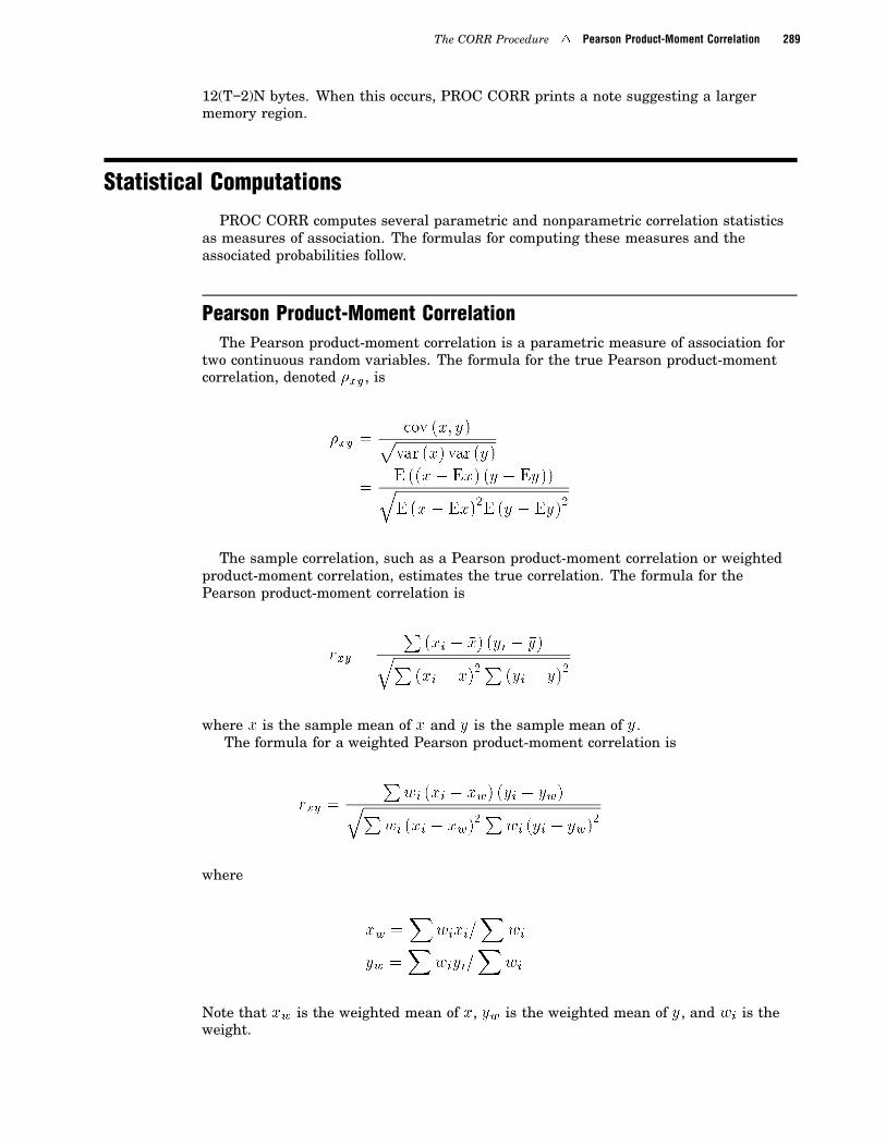
Statistical Computations

PROC CORR computes several parametric and nonparametric correlation statisticsas measures of association. The formulas for computing these measures and theassociated probabilities follow.

Pearson Product-Moment CorrelationThe Pearson product-moment correlation is a parametric measure of association for

two continuous random variables. The formula for the true Pearson product-momentcorrelation, denoted �xy, is

�xy =cov (x; y)pvar (x) var (y)

=E ((x� Ex) (y � Ey))qE (x � Ex)2E (y � Ey)2

The sample correlation, such as a Pearson product-moment correlation or weightedproduct-moment correlation, estimates the true correlation. The formula for thePearson product-moment correlation is

rxy =

P(xi � �x) (yi � �y)qP

(xi � �x)2P

(yi � �y)2

where �x is the sample mean of x and �y is the sample mean of y.The formula for a weighted Pearson product-moment correlation is

rxy =

Pwi (xi � �xw) (yi � �yw)qP

wi (xi � �xw)2P

wi (yi � �yw)2

where

�xw =X

wixi=X

wi

�yw =X

wiyi=X

wi

Note that �xw is the weighted mean of x, �yw is the weighted mean of y, and wi is theweight.

290 Spearman Rank-Order Correlation 4 Chapter 12

When one variable is dichotomous (0,1) and the other variable is continuous, aPearson correlation is equivalent to a point biserial correlation. When both variablesare dichotomous, a Pearson correlation coefficient is equivalent to the phi coefficient.

Spearman Rank-Order CorrelationSpearman rank-order correlation is a nonparametric measure of association based on

the rank of the data values. The formula is

� =

P �Ri �

�R� �

Si ��S�

qP�Ri �

�R�2P�

Si ��S�2

where Ri is the rank of the ith x value, Si is the rank of the ith y value, �R is themean of the Ri values, and �S is the mean of the Si values.

PROC CORR computes the Spearman’s correlation by ranking the data and usingthe ranks in the Pearson product-moment correlation formula. In case of ties, theaveraged ranks are used.

Kendall’s tau-bKendall’s tau-b is a nonparametric measure of association based on the number of

concordances and discordances in paired observations. Concordance occurs when pairedobservations vary together, and discordance occurs when paired observations varydifferently. The formula for Kendall’s tau-b is

� =

Pi<j

sgn (xi � xj ) sgn (yi � yj )p(T0 � T1) (T0 � T2)

where

T0 = n (n � 1) =2

T1 =X

ti (ti � 1) =2

T2 =X

ui (ui � 1) =2

and where ti is the number of tied x values in the ith group of tied x values, ui is thenumber of tied y values in the ith group of tied y values, f is the number ofobservations, and sgn(z) is defined as

sgn (z) =

(1 if z > 00 if z = 0

�1 if z < 0

PROC CORR computes Kendall’s correlation by ranking the data and using a methodsimilar to Knight (1966). The data are double sorted by ranking observations according

The CORR Procedure 4 Partial Correlation 291

to values of the first variable and reranking the observations according to values of thesecond variable. PROC CORR computes Kendall’s tau-b from the number ofinterchanges of the first variable and corrects for tied pairs (pairs of observations withequal values of X or equal values of Y).

Hoeffding’s Measure of Dependence, DHoeffding’s measure of dependence, D, is a nonparametric measure of association

that detects more general departures from independence. The statistic approximates aweighted sum over observations of chi-square statistics for two-by-two classificationtables (Hoeffding 1948). Each set of (x; y) values are cut points for the classification.The formula for Hoeffding’s D is

D = 30(n � 2) (n� 3)D1 +D2 � 2 (n � 2) D3

n (n � 1) (n � 2) (n � 3) (n � 4)

where

D1 =X

i

(Qi � 1) (Qi � 2)

D2 =X

i

(Ri � 1) (Ri � 2) (Si � 1) (Si � 2)

D3 =X

i

(Ri � 2) (Si � 2) (Qi � 1)

Ri is the rank of xi, Si is the rank of yi, and Qi (also called the bivariate rank) is 1plus the number of points with both x and y values less than the ith point. A pointthat is tied on only the x value or y value contributes 1/2 to Qi if the other value is lessthan the corresponding value for the ith point. A point that is tied on both x and ycontributes 1/4 to Qi .

PROC CORR obtains the Qi values by first ranking the data. The data are thendouble sorted by ranking observations according to values of the first variable andreranking the observations according to values of the second variable. Hoeffding’s Dstatistic is computed using the number of interchanges of the first variable.

When no ties occur among data set observations, the D statistic values are between-0.5 and 1, with 1 indicating complete dependence. However, when ties occur, the Dstatistic may result in a smaller value. That is, for a pair of variables with identicalvalues, the Hoeffding’s D statistic may be less than 1. With a large number of ties in asmall data set, the D statistic may be less than -0.5 . For more information onHoeffding’s D, see Hollander and Wolfe (1973, p. 228).

Partial CorrelationA partial correlation measures the strength of a relationship between two variables,

while controlling the effect of one or more additional variables. The Pearson partialcorrelation for a pair of variables may be defined as the correlation of errors afterregression on the controlling variables. Let y= (y1 ;y2 ; . . . ; yv ) be the set of variablesto correlate. Also let � and � be sets of regression parameters and z be the set of

292 Partial Correlation 4 Chapter 12

controlling variables, where � =(�1; �2; . . . ; �v), � is the slope, andz= (z1 ; z2 ; . . . ; zp). Suppose

E (y) = �+ z�

is a regression model for y given z. The population Pearson partial correlation betweenthe ith and the jth variables of y given z is defined as the correlation between errors(yi � E (yi )) and (yj � E (yj )).

If the exact values of � and � are unknown, you can use a sample Pearson partialcorrelation to estimate the population Pearson partial correlation. For a given sampleof observations, you estimate the sets of unknown parameters � and � using theleast-squares estimators b� and b�. Then the fitted least-squares regression model is

by = b�+ zb�The partial corrected sums of squares and crossproducts (CSSCP) of y given z are

the corrected sums of squares and crossproducts of the residuals y� by. Using thesepartial corrected sums of squares and crossproducts, you can calculate the partialvariances, partial covariances, and partial correlations.

PROC CORR derives the partial corrected sums of squares and crossproducts matrixby applying the Cholesky decomposition algorithm to the CSSCP matrix. For Pearsonpartial correlations, let S be the partitioned CSSCP matrix between two sets ofvariables, z and y:

S =

�Szz SzyS0

zySyy

�

PROC CORR calculates Syy�z, the partial CSSCP matrix of y after controlling for z,by applying the Cholesky decomposition algorithm sequentially on the rows associatedwith z, the variables being partialled out.

After applying the Cholesky decomposition algorithm to each row associated withvariables z, PROC CORR checks all higher numbered diagonal elements associatedwith z for singularity. After the Cholesky decomposition, a variable is consideredsingular if the value of the corresponding diagonal element is less than p times theoriginal unpartialled corrected sum of squares of that variable. You can specify thesingularity criterion p using the SINGULAR= option. For Pearson partial correlations,a controlling variable z is considered singular if the R2 for predicting this variable fromthe variables that are already partialled out exceeds 1� p. When this happens, PROCCORR excludes the variable from the analysis. Similarly, a variable is consideredsingular if the R2 for predicting this variable from the controlling variables exceeds1 � p. When this happens, its associated diagonal element and all higher numberedelements in this row or column are set to zero.

After the Cholesky decomposition algorithm is performed on all rows associated withz, the resulting matrix has the form

�Tzz Tzy

0 Syy�z

�

where Tzz is an upper triangular matrix with

The CORR Procedure 4 Cronbach’s Coefficient Alpha 293

T0

zzTzz = Szz0

T0

zzTzy = Szy0

Syy�z = Syy �T0

zyTzy:

If Szz is positive definite, then the partial CSSCP matrix Syy�z is identical to thematrix derived from the formula

Syy�z = Syy � S0

zy S�1zz Szy

The partial variance-covariance matrix is calculated with the variance divisor(VARDEF= option). PROC CORR can then use the standard Pearson correlationformula on the partial variance-covariance matrix to calculate the Pearson partialcorrelation matrix. Another way to calculate Pearson partial correlation is by applyingthe Cholesky decomposition algorithm directly to the correlation matrix and by usingthe correlation formula on the resulting matrix.

To derive the corresponding Spearman partial rank-order correlations and Kendallpartial tau-b correlations, PROC CORR applies the Cholesky decomposition algorithmto the Spearman rank-order correlation matrix and Kendall tau-b correlation matrixand uses the correlation formula. The singularity criterion for nonparametric partialcorrelations is identical to Pearson partial correlation except that PROC CORR uses amatrix of nonparametric correlations and sets a singular variable’s associatedcorrelations to missing. The partial tau-b correlations range from –1 to 1. However, thesampling distribution of this partial tau-b is unknown; therefore, the probability valuesare not available.

When a correlation matrix (Pearson, Spearman, or Kendall tau-b correlation matrix)is positive definite, the resulting partial correlation between variables x and y afteradjusting for a single variable z is identical to that obtained from the first-order partialcorrelation formula

rxy�z =rxy � rxzryzq

(1 � r2xz)�1� r2

yz

�

where rxy, rxz, and ryz are the appropriate correlations.The formula for higher-order partial correlations is a straightforward extension of

the above first-order formula. For example, when the correlation matrix is positivedefinite, the partial correlation between x and y controlling for both z1 and z2 isidentical to the second-order partial correlation formula

rxy�z1z2 =rxy�z1 � rxz2�z1ryz2�z1q�1 � r2

xz2�z1

� �1� r2

yz2�z1

�

where rxy�z1, rxz2�z1, and ryz2�z1 are first-order partial correlations among variables x,y, and z2 given z1.

Cronbach’s Coefficient AlphaAnalyzing latent constructs such as job satisfaction, motor ability, sensory

recognition, or customer satisfaction requires instruments to accurately measure the

294 Cronbach’s Coefficient Alpha 4 Chapter 12

constructs. Interrelated items may be summed to obtain an overall score for eachparticipant. Cronbach’s coefficient alpha estimates the reliability of this type of scale bydetermining the internal consistency of the test or the average correlation of itemswithin the test (Cronbach 1951).

When a value is recorded, the observed value contains some degree of measurementerror. Two sets of measurements on the same variable for the same individual may nothave identical values. However, repeated measurements for a series of individuals willshow some consistency. Reliability measures internal consistency from one set ofmeasurements to another. The observed value Y is divided into two components, a truevalue T and a measurement error E. The measurement error is assumed to beindependent of the true value, that is,

Y = T+ E ; cov (T;E) = 0

The reliability coefficient of a measurement test is defined as the squared correlationbetween the observed value Y and the true value T, that is,

�2 (Y;T) =cov (Y;T)2

var (Y) var (T)

=var (T)2

var (Y) var (T)

=var (T)

var (Y)

which is the proportion of the observed variance due to true differences amongindividuals in the sample. If Y is the sum of several observed variables measuring thesame feature, you can estimate var(T). Cronbach’s coefficient alpha, based on a lowerbound for var(T), is an estimate of the reliability coefficient.

Suppose p variables are used with Yj = Tj + Ej for j = 1; 2; . . . ; p, where Yj isthe observed value, Tj is the true value, and Ej is the measurement error. Themeasurement errors (Ej ) are independent of the true values (Tj ) and are alsoindependent of each other. Let Y0 =

PYj be the total observed score and T0 =

PTj

be the total true score. Because

(p� 1)X

var (Tj ) �X

i 6=j

cov (Ti ;Tj ) ;

a lower bound for var (T0) is given by

p

p� 1

X

i 6=j

cov (Ti ;Tj )

With cov (Yi ;Yj ) = cov (Ti ;Tj ) for i 6= j, a lower bound for the reliabilitycoefficient is then given by the Cronbach’s coefficient alpha:

The CORR Procedure 4 Probability Values 295

� =

�p

p � 1

� Pi 6=j

cov (Yi ;Yj )

var (Y0)

=

�p

p � 1

�0B@1 �

Pjvar (Yj )

var (Y0)

1CA

If the variances of the items vary widely, you can standardize the items to a standarddeviation of 1 before computing the coefficient alpha. If the variables are dichotomous(0,1), the coefficient alpha is equivalent to the Kuder-Richardson 20 (KR-20) reliabilitymeasure.

When the correlation between each pair of variables is 1, the coefficient alpha has amaximum value of 1. With negative correlations between some variables, the coefficientalpha can have a value less than zero. The larger the overall alpha coefficient, the morelikely that items contribute to a reliable scale. Nunnally (1978) suggests .70 as anacceptable reliability coefficient; smaller reliability coefficients are seen as inadequate.However, this varies by discipline.

To determine how each item reflects the reliability of the scale, you calculate acoefficient alpha after deleting each variable independently from the scale. TheCronbach’s coefficient alpha from all variables except the kth variable is given by

�k =

�p � 1

p � 2

�0BBBB@1�

Pi 6=k

var (Yi)

var

Pi 6=k

Yi

!1CCCCA

If the reliability coefficient increases after deleting an item from the scale, you canassume that the item is not correlated highly with other items in the scale. Conversely,if the reliability coefficient decreases you can assume that the item is highly correlatedwith other items in the scale. See SAS Communications, 4th Quarter 1994, for moreinformation on how to interpret Cronbach’s coefficient alpha.

Listwise deletion of observations with missing values is necessary to correctlycalculate Cronbach’s coefficient alpha. PROC CORR does not automatically use listwisedeletion when you specify ALPHA. Therefore, use the NOMISS option if the data setcontains missing values. Otherwise, PROC FREQ prints a warning message in the SASlog indicating the need to use NOMISS with ALPHA.

Probability ValuesProbability values for the Pearson and Spearman correlations are computed by

treating

(n� 2)1=2 r

(1 � r2)1=2

296 Probability Values 4 Chapter 12

as coming from a t distribution with n � 2 degrees of freedom, where r is theappropriate correlation.

Probability values for the Pearson and Spearman partial correlations are computedby treating

(n� k � 2)1=2 r

(1� r2)1=2

as coming from a t distribution with n � k � 2 degrees of freedom, where r is theappropriate partial correlation and k is the number of variables being partialled out.

Probability values for Kendall correlations are computed by treating

spvar (s)

as coming from a normal distribution when

s =Xi<j

sgn (xi � xj ) sgn (yi � yj )

and where xi are the values of the first variable, yi are the values of the secondvariable, and the function sgn(z) is defined as

sgn (z) =

(1 if z > 00 if z = 0

�1 if z < 0

The formula for the variance of s, var(s), is computed as

var (s) =v0 � vt � vu

18+

v12n (n� 1)

+v2

9n (n� 1) (n� 2)

wherev0 = n (n� 1) (2n+ 5)vt =

Pti (ti � 1) (2ti + 5)

vu =P

ui (ui � 1) (2ui + 5)v1 = (

Pti (ti � 1)) (

Pui (ui � 1))

v2 = (P

ti (ti � 1) (ti � 2)) (P

ui (ui � 1) (ui � 2))

The sums are over tied groups of values where ti is the number of tied x values andui is the number of tied y values (Noether 1967). The sampling distribution ofKendall’s partial tau-b is unknown; therefore, the probability values are not available.

The probability values for Hoeffding’s D statistic are computed using the asymptoticdistribution computed by Blum, Kiefer, and Rosenblatt (1961). The formula is

(n� 1)�4

60D +

�4

72

The CORR Procedure 4 Procedure Output 297

which comes from the asymptotic distribution. When the sample size is less than 10,see the tables for the distribution of D in Hollander and Wolfe (1973).

Results

Missing ValuesBy default, PROC CORR uses pairwise deletion when observations contain missing

values. PROC CORR includes all nonmissing pairs of values for each pair of variablesin the statistical computations. Therefore, the correlations statistics may be based ondifferent numbers of observations.

If you specify the NOMISS option, PROC CORR uses listwise deletion when a valueof the BY, FREQ, VAR, WEIGHT, or WITH statement variable is missing. PROC CORRexcludes all observations with missing values from the analysis. Therefore, the numberof observations for each pair of variables is identical. The PARTIAL statement alwaysexcludes the observations with missing values by automatically invoking NOMISS.Listwise deletion is needed to correctly calculate Cronbach’s coefficient alpha when dataare missing. If a data set contains missing values, when you specify ALPHA use theNOMISS option

There are two reasons to specify NOMISS and, thus, to avoid pairwise deletion.First, NOMISS is computationally more efficient, so you use fewer computer resources.Second, if you use the correlations as input to regression or other statistical procedures,a pairwise-missing correlation matrix leads to several statistical difficulties. Pairwisecorrelation matrices may not be nonnegative definite, and the pattern of missing valuesmay bias the results.

Procedure OutputBy default, PROC CORR prints a report that includes descriptive statistics and

correlation statistics for each variable.The descriptive statistics include the number ofobservations with nonmissing values, the mean, the standard deviation, the minimum,and the maximum. PROC CORR reports the following additional descriptive statisticswhen you request various correlation statistics:

sumfor Pearson correlation only

medianfor nonparametric measures of association

partial variancefor Pearson partial correlation

partial standard deviationfor Pearson partial correlation.

If variable labels are available, PROC CORR labels the variables.When you specify the CSSCP, SSCP, or COV option, the appropriate sum-of-squares

and crossproducts and covariance matrix appears at the top of the correlation report. Ifthe data set contains missing values, PROC CORR prints additional statistics for eachpair of variables. These statistics, calculated from the observations with nonmissingrow and column variable values, may include

SSCP(W’,’V’)uncorrected sum-of-squares and crossproducts

298 Output Data Sets 4 Chapter 12

USS(W’)uncorrected sum-of-squares for the row variable

USS(V’)uncorrected sum-of-squares for the column variable

CSSCP(W’,’V’)corrected sum-of-squares and crossproducts

CSS(W’)corrected sum-of-squares for the row variable

CSS(V’)corrected sum-of-squares for the column variable

COV (W’,’V’)covariance

VAR (W’)variance for the row variable

VAR (V’)variance for the column variable

DF(W’,V’)divisor for calculating covariance and variances.

For each pair of variables, PROC CORR always prints the correlation coefficients, thenumber of observations used to calculate the coefficient, and the significance probability.When you specify the ALPHA option, PROC CORR prints Cronbach’s coefficient alpha,the correlation between the variable and the total of the remaining variables, andCronbach’s coefficient alpha using the remaining variables for the raw variables andthe standardized variables.

Output Data SetsWhen you specify the OUTP=, OUTS=, OUTK=, or OUTH= option, PROC CORR

creates an output data set containing statistics for Pearson correlation, Spearmancorrelation, Kendall correlation, or Hoeffding’s D, respectively. By default, the outputdata set is a special data set type (TYPE=CORR) that many SAS/STAT proceduresrecognize, including PROC REG and PROC FACTOR. When you specify the NOCORRoption and the COV, CSSCP, or SSCP option, use the TYPE= data set option to changethe data set type to COV, CSSCP, or SSCP. For example, the following statement

proc corr nocorr cov outp=b(type=cov);

specifies the output data set type as COV.PROC CORR does not print the output data set. Use PROC PRINT, PROC REPORT,

or another SAS reporting tool to print the output data set.The output data set includes the following variables

BY variablesidentifies the BY group when using a BY statement.

_TYPE_ variableidentifies the type of observation.

_NAME_ variableidentifies the variable that corresponds to a given row of the correlation matrix.

INTERCEP variableidentifies variable sums when specifying the SSCP option.

The CORR Procedure 4 Output Data Sets 299

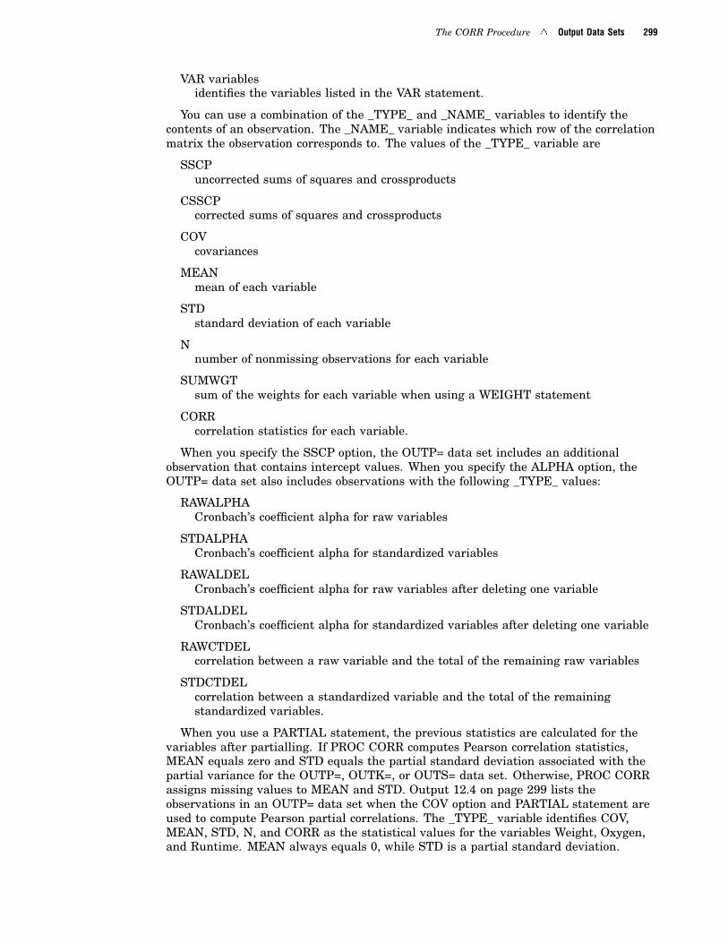
VAR variablesidentifies the variables listed in the VAR statement.

You can use a combination of the _TYPE_ and _NAME_ variables to identify thecontents of an observation. The _NAME_ variable indicates which row of the correlationmatrix the observation corresponds to. The values of the _TYPE_ variable are

SSCPuncorrected sums of squares and crossproducts

CSSCPcorrected sums of squares and crossproducts

COVcovariances

MEANmean of each variable

STDstandard deviation of each variable

Nnumber of nonmissing observations for each variable

SUMWGTsum of the weights for each variable when using a WEIGHT statement

CORRcorrelation statistics for each variable.

When you specify the SSCP option, the OUTP= data set includes an additionalobservation that contains intercept values. When you specify the ALPHA option, theOUTP= data set also includes observations with the following _TYPE_ values:

RAWALPHACronbach’s coefficient alpha for raw variables

STDALPHACronbach’s coefficient alpha for standardized variables

RAWALDELCronbach’s coefficient alpha for raw variables after deleting one variable

STDALDELCronbach’s coefficient alpha for standardized variables after deleting one variable

RAWCTDELcorrelation between a raw variable and the total of the remaining raw variables

STDCTDELcorrelation between a standardized variable and the total of the remainingstandardized variables.

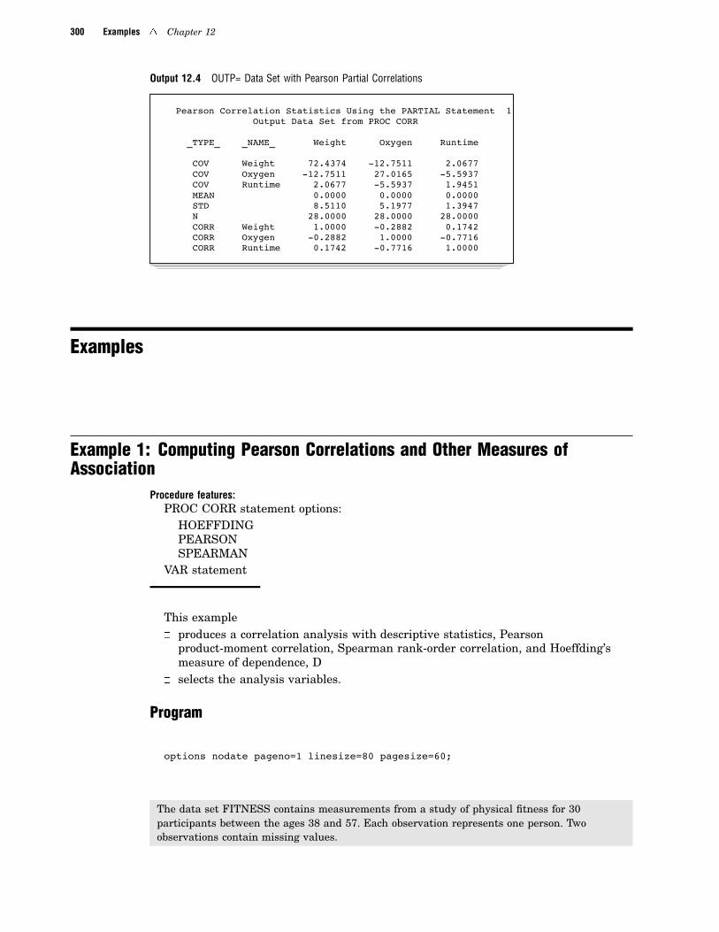
When you use a PARTIAL statement, the previous statistics are calculated for thevariables after partialling. If PROC CORR computes Pearson correlation statistics,MEAN equals zero and STD equals the partial standard deviation associated with thepartial variance for the OUTP=, OUTK=, or OUTS= data set. Otherwise, PROC CORRassigns missing values to MEAN and STD. Output 12.4 on page 299 lists theobservations in an OUTP= data set when the COV option and PARTIAL statement areused to compute Pearson partial correlations. The _TYPE_ variable identifies COV,MEAN, STD, N, and CORR as the statistical values for the variables Weight, Oxygen,and Runtime. MEAN always equals 0, while STD is a partial standard deviation.

300 Examples 4 Chapter 12

Output 12.4 OUTP= Data Set with Pearson Partial Correlations

Pearson Correlation Statistics Using the PARTIAL Statement 1Output Data Set from PROC CORR

_TYPE_ _NAME_ Weight Oxygen Runtime

COV Weight 72.4374 -12.7511 2.0677COV Oxygen -12.7511 27.0165 -5.5937COV Runtime 2.0677 -5.5937 1.9451MEAN 0.0000 0.0000 0.0000STD 8.5110 5.1977 1.3947N 28.0000 28.0000 28.0000CORR Weight 1.0000 -0.2882 0.1742CORR Oxygen -0.2882 1.0000 -0.7716CORR Runtime 0.1742 -0.7716 1.0000

Examples

Example 1: Computing Pearson Correlations and Other Measures ofAssociation

Procedure features:PROC CORR statement options:

HOEFFDINGPEARSONSPEARMAN

VAR statement

This example� produces a correlation analysis with descriptive statistics, Pearson

product-moment correlation, Spearman rank-order correlation, and Hoeffding’smeasure of dependence, D

� selects the analysis variables.

Program

options nodate pageno=1 linesize=80 pagesize=60;

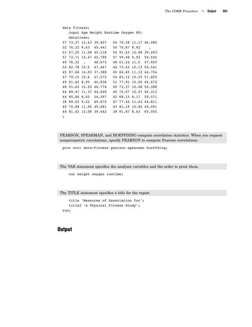
The data set FITNESS contains measurements from a study of physical fitness for 30participants between the ages 38 and 57. Each observation represents one person. Twoobservations contain missing values.

The CORR Procedure 4 Output 301

data fitness;input Age Weight Runtime Oxygen @@;datalines;

57 73.37 12.63 39.407 54 79.38 11.17 46.08052 76.32 9.63 45.441 50 70.87 8.92 .51 67.25 11.08 45.118 54 91.63 12.88 39.20351 73.71 10.47 45.790 57 59.08 9.93 50.54549 76.32 . 48.673 48 61.24 11.5 47.92052 82.78 10.5 47.467 44 73.03 10.13 50.54145 87.66 14.03 37.388 45 66.45 11.12 44.75447 79.15 10.6 47.273 54 83.12 10.33 51.85549 81.42 8.95 40.836 51 77.91 10.00 46.67248 91.63 10.25 46.774 49 73.37 10.08 50.38844 89.47 11.37 44.609 40 75.07 10.07 45.31344 85.84 8.65 54.297 42 68.15 8.17 59.57138 89.02 9.22 49.874 47 77.45 11.63 44.81140 75.98 11.95 45.681 43 81.19 10.85 49.09144 81.42 13.08 39.442 38 81.87 8.63 60.055;

PEARSON, SPEARMAN, and HOEFFDING compute correlation statistics. When you requestnonparametric correlations, specify PEARSON to compute Pearson correlations.

proc corr data=fitness pearson spearman hoeffding;

The VAR statement specifies the analysis variables and the order to print them.

var weight oxygen runtime;

The TITLE statement specifies a title for the report.

title ’Measures of Association for’;title2 ’a Physical Fitness Study’;

run;

Output

302 Output 4 Chapter 12

The correlation report includes descriptive statistics, Pearson’s rho, Spearman’s rho, andHoeffding’s D. The report uses the median, instead of the sum, as a descriptive measure whenPROC CORR computes nonparametric measures of association.

Because missing data are excluded pairwise, the number of observations PROC CORR uses tocalculate the correlation coefficients varies.

Measures of Association for 1a Physical Fitness Study

The CORR Procedure


Simple Statistics

Variable N Mean Std Dev Median Minimum Maximum

Weight 30 77.70500 8.34152 77.68000 59.08000 91.63000Oxygen 29 47.06445 5.32129 46.67200 37.38800 60.05500Runtime 29 10.61448 1.41655 10.47000 8.17000 14.03000




Weight 1.00000 -0.19900 0.151550.3007 0.4326

30 29 29

Oxygen -0.19900 1.00000 -0.783460.3007 <.0001

29 29 28

Runtime 0.15155 -0.78346 1.000000.4326 <.0001

29 28 29

Spearman Correlation CoefficientsProb > |r| under H0: Rho=0



Weight 1.00000 -0.13110 0.105460.4979 0.5861

30 29 29

Oxygen -0.13110 1.00000 -0.683630.4979 <.0001

29 29 28

Runtime 0.10546 -0.68363 1.000000.5861 <.0001

29 28 29

The CORR Procedure 4 Program 303

Measures of Association for 2a Physical Fitness Study

The CORR Procedure

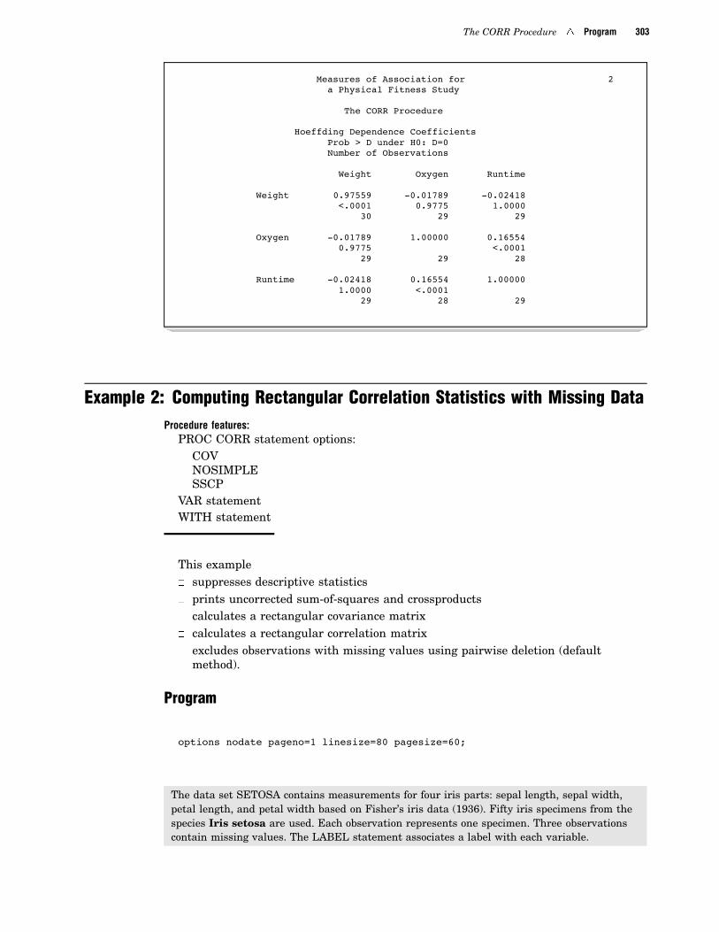
Hoeffding Dependence CoefficientsProb > D under H0: D=0Number of Observations


Weight 0.97559 -0.01789 -0.02418<.0001 0.9775 1.0000

30 29 29

Oxygen -0.01789 1.00000 0.165540.9775 <.0001

29 29 28

Runtime -0.02418 0.16554 1.000001.0000 <.0001

29 28 29

Example 2: Computing Rectangular Correlation Statistics with Missing DataProcedure features:

PROC CORR statement options:COVNOSIMPLESSCP

VAR statementWITH statement

This example� suppresses descriptive statistics� prints uncorrected sum-of-squares and crossproducts� calculates a rectangular covariance matrix� calculates a rectangular correlation matrix� excludes observations with missing values using pairwise deletion (default

method).

Program


The data set SETOSA contains measurements for four iris parts: sepal length, sepal width,petal length, and petal width based on Fisher’s iris data (1936). Fifty iris specimens from thespecies Iris setosa are used. Each observation represents one specimen. Three observationscontain missing values. The LABEL statement associates a label with each variable.


data setosa;input SepalLength SepalWidth PetalLength PetalWidth @@;label sepallength=’Sepal Length in mm.’

sepalwidth=’Sepal Width in mm.’petallength=’Petal Length in mm.’petalwidth=’Petal Width in mm.’;

datalines;50 33 14 02 46 34 14 03 46 36 . 0251 33 17 05 55 35 13 02 48 31 16 0252 34 14 02 49 36 14 01 44 32 13 0250 35 16 06 44 30 13 02 47 32 16 0248 30 14 03 51 38 16 02 48 34 19 0250 30 16 02 50 32 12 02 43 30 11 .58 40 12 02 51 38 19 04 49 30 14 0251 35 14 02 50 34 16 04 46 32 14 0257 44 15 04 50 36 14 02 54 34 15 0452 41 15 . 55 42 14 02 49 31 15 0254 39 17 04 50 34 15 02 44 29 14 0247 32 13 02 46 31 15 02 51 34 15 0250 35 13 03 49 31 15 01 54 37 15 0254 39 13 04 51 35 14 03 48 34 16 0248 30 14 01 45 23 13 03 57 38 17 0351 38 15 03 54 34 17 02 51 37 15 0452 35 15 02 53 37 15 02;

SSCP displays the uncorrected sum-of-squares and crossproducts matrix and invokesPEARSON. COV calculates the covariance matrix. NOSIMPLE suppresses descriptive statistics.

proc corr data=setosa sscp cov nosimple;

The WITH statement together with the VAR statement produces a rectangular correlationmatrix. The matrix rows are PetalLength and PetalWidth while the matrix columns areSepalLength and SepalWidth.

var sepallength sepalwidth;with petallength petalwidth;


title ’Fisher (1936) Iris Setosa Data’;run;

Output


The correlation report includes rectangular sum-of-squares and crossproducts, covariances, andthe correlation matrix using the two WITH variables and two VAR variables. The descriptivestatistics do not appear. PROC CORR uses variable labels to label matrix rows (WITHvariables).

PROC CORR calculates sum-of-squares and crossproducts and covariances statistics for eachpair of variables by using observations with nonmissing row and column variable values.

Because missing data are excluded pairwise, the number of observations PROC CORR uses tocalculate the correlation coefficients changes.

Fisher (1936) Iris Setosa Data 1

The CORR Procedure

2 With Variables: PetalLength PetalWidth2 Variables: SepalLength SepalWidth

Sums of Squares and CrossproductsSSCP / Row Var SS / Col Var SS

SepalLength SepalWidth

PetalLength 36214.00000 24756.00000Petal Length in mm. 10735.00000 10735.00000

123793.0000 58164.0000

PetalWidth 6113.00000 4191.00000Petal Width in mm. 355.00000 355.00000

121356.0000 56879.0000

Variances and CovariancesCovariance / Row Var Variance / Col Var Variance / DF

SepalLength SepalWidth


12.33333333 14.6054421848 48


11.80141844 13.6272163147 47



Sepal SepalLength Width


49 49


48 48

306 Example 3: Computing Cronbach’s Coefficient Alpha 4 Chapter 12

Example 3: Computing Cronbach’s Coefficient AlphaProcedure features:

PROC CORR statement options:ALPHANOCORRNOMISS

This example� computes Cronbach’s coefficient alpha for a multiple-item mixed-rating scale� suppresses Pearson correlation statistics� excludes observations with missing values using listwise deletion.

This example does not examine the correlation matrix but assumes that all items arepositively correlated. Normally, you want to examine the correlation and covariancematrices to make sure that all variables are positively correlated. Positive correlation isneeded because items measure a common entity. You exclude negatively correlateditems from the analysis because they do not measure the same construct.

Program


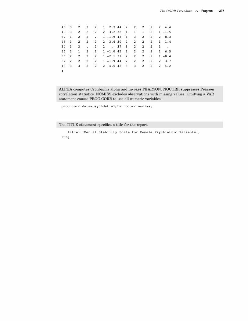
The data set PYSCHDAT contains responses to a questionnaire assessing the mental stability of30 randomly selected female psychiatric patients.* Each observation represents one patient. Thescale includes seven items. The LABEL statement provides a label for each item. Sevenobservations contain missing values.

data psychdat;input Age Anxiety Depression Sleep Sex Life WeightChange @@;label age = ’age in years’

anxiety = ’anxiety level’depression = ’depression level’sleep = ’normal sleep (1=y 2=n)’sex = ’sexual (1=n 2=y)’life = ’suicidal (1=n 2=y)’weightchange = ’recent weight change’;

datalines;39 2 2 2 2 2 4.9 41 2 2 2 2 2 2.242 3 3 . 2 2 4.0 30 2 2 2 2 2 -2.635 2 1 1 2 1 -0.3 44 . 1 2 1 1 0.931 2 2 . 2 2 -1.5 39 3 2 2 2 1 3.535 3 2 2 2 2 -1.2 33 2 2 2 2 2 0.838 2 1 1 1 1 -1.9 31 2 2 2 . 1 5.5

*Data are from Assignments in Applied Statistics by Simon Conrad. Copyright ©1989, by John Wiley & Sons, Inc. Reprintedwith permission from the publisher.

The CORR Procedure 4 Program 307

40 3 2 2 2 1 2.7 44 2 2 2 2 2 4.443 3 2 2 2 2 3.2 32 1 1 1 2 1 -1.532 1 2 2 . 1 -1.9 43 4 3 2 2 2 8.346 3 2 2 2 2 3.6 30 2 2 2 2 1 1.434 3 3 . 2 2 . 37 3 2 2 2 1 .35 2 1 2 2 1 -1.0 45 2 2 2 2 2 6.535 2 2 2 2 1 -2.1 31 2 2 2 2 1 -0.432 2 2 2 2 1 -1.9 44 2 2 2 2 2 3.740 3 3 2 2 2 4.5 42 3 3 2 2 2 4.2;

ALPHA computes Cronbach’s alpha and invokes PEARSON. NOCORR suppresses Pearsoncorrelation statistics. NOMISS excludes observations with missing values. Omitting a VARstatement causes PROC CORR to use all numeric variables.

proc corr data=psychdat alpha nocorr nomiss;


title1 ’Mental Stability Scale for Female Psychiatric Patients’;run;


Output

The correlation report includes descriptive statistics and Cronbach’s coefficient alpha, thecorrelation between the variable and the total of the remaining variables, and Cronbach’scoefficient alpha using the remaining variables for both the raw variables and the standardizedvariables. These calculations use the 23 observations without missing values.

Because the variances of some variables vary widely, you use the standardized scores toestimate reliability. The overall standardized alpha of .85 is an acceptable reliability coefficient.This is greater than Nunnally’s suggested value of .70.

The standardized alpha provides information on how each item reflects the reliability of thescale. Notice that the standardized alpha decreases after removing Depression from theconstruct. Therefore, this variable appears strongly correlated with other items in the scale.The standardized alpha increases slightly after removing Sex from the construct. Thus,removing this variable from the scale makes the construct more reliable.

Mental Stability Scale for Female Psychiatric Patients 1

The CORR Procedure

7 Variables: Age Anxiety Depression Sleep SexLife WeightChange

Simple Statistics

Variable N Mean Std Dev Sum

Age 23 37.91304 5.13378 872.00000Anxiety 23 2.34783 0.64728 54.00000Depression 23 1.95652 0.56232 45.00000Sleep 23 1.86957 0.34435 43.00000Sex 23 1.95652 0.20851 45.00000Life 23 1.56522 0.50687 36.00000WeightChange 23 1.78261 3.06381 41.00000

Simple Statistics

Variable Minimum Maximum Label

Age 30.00000 46.00000 age in yearsAnxiety 1.00000 4.00000 anxiety levelDepression 1.00000 3.00000 depression levelSleep 1.00000 2.00000 normal sleep (1=y 2=n)Sex 1.00000 2.00000 sexual (1=n 2=y)Life 1.00000 2.00000 suicidal (1=n 2=y)WeightChange -2.60000 8.30000 recent weight change

Cronbach Coefficient Alpha

Variables Alpha----------------------------Raw 0.627754Standardized 0.845339

The CORR Procedure 4 Example 4: Storing Partial Correlations in an Output Data Set 309

Mental Stability Scale for Female Psychiatric Patients 2

The CORR Procedure

Cronbach Coefficient Alpha with Deleted Variable

Raw Variables Standardized Variables

Deleted Correlation CorrelationVariable with Total Alpha with Total Alpha----------------------------------------------------------------------------Age 0.742614 0.557515 0.546856 0.832207


DeletedVariable Label--------------------------------------Age age in years


Raw Variables Standardized Variables

Deleted Correlation CorrelationVariable with Total Alpha with Total Alpha----------------------------------------------------------------------------Anxiety 0.577129 0.600944 0.590851 0.825643Depression 0.554983 0.608273 0.770956 0.797610Sleep 0.378930 0.630242 0.618367 0.821482Sex 0.155115 0.642017 0.333368 0.862537Life 0.622207 0.607333 0.625338 0.820421WeightChange 0.843939 0.341006 0.749261 0.801087


DeletedVariable Label--------------------------------------Anxiety anxiety levelDepression depression levelSleep normal sleep (1=y 2=n)Sex sexual (1=n 2=y)Life suicidal (1=n 2=y)WeightChange recent weight change

Example 4: Storing Partial Correlations in an Output Data Set

Procedure features:PROC CORR statement options:

COVKENDALLNOSIMPLEOUTP=SPEARMAN

PARTIAL statementVAR statement

310 Program 4 Chapter 12

Data set: FITNESS on page 301

This example� suppresses descriptive statistics� calculates three types of partial correlation coefficients� calculates a partial covariance matrix� excludes observations with missing values using listwise deletion� selects the analysis variables� creates an output data set with Pearson correlation statistics.

See Output 12.4 on page 299 for a listing of the output data set.

Program


SPEARMAN and KENDALL request correlation statistics. COV calculates the covariancematrix and invokes PEARSON. NOSIMPLE suppresses descriptive statistics. OUT= creates theFITCORR data set that contains Pearson correlation statistics.

proc corr data=fitness spearman kendall cov nosimpleoutp=fitcorr;

The VAR statement specifies the analysis variables and the order to print them.

var weight oxygen runtime;

The PARTIAL statement calculates partial correlations using Age as the controlling variable.

partial age;

The LABEL statement associates a label with each variable for the duration of the PROC step.

label age = ’Age of subject’weight = ’Wt in kg’runtime = ’1.5 mi in minutes’oxygen = ’O2 use’;


title1 ’Partial Correlations for a Fitness and Exercise Study’;run;


Output

The report includes a partial covariance matrix and partial correlations for Pearson’s rho, Spearman’s rho, andKendall’s tau-b. The p-values for Kendall’s tau-b are not available. Because observations with missing data areexcluded, PROC CORR uses 28 observations to calculate correlation coefficients.

Partial Correlations for a Fitness and Exercise Study 1

The CORR Procedure

1 Partial Variables: Age


Partial Covariance Matrix, DF = 26


Weight Wt in kg 72.43742055 -12.75113194 2.06766763

Oxygen O2 use -12.75113194 27.01654904 -5.59370556

Runtime 1.5 mi in minutes 2.06766763 -5.59370556 1.94512451

Pearson Partial Correlation Coefficients, N = 28



Weight 1.00000 -0.28824 0.17419

Wt in kg 0.1448 0.3849

Oxygen -0.28824 1.00000 -0.77163

O2 use 0.1448 <.0001

Runtime 0.17419 -0.77163 1.00000

1.5 mi in minutes 0.3849 <.0001

Spearman Partial Correlation Coefficients, N = 28



Weight 1.00000 -0.16407 0.08708

Wt in kg 0.4135 0.6658

Oxygen -0.16407 1.00000 -0.67112

O2 use 0.4135 0.0001

Runtime 0.08708 -0.67112 1.00000

1.5 mi in minutes 0.6658 0.0001

Kendall Partial Tau b Correlation Coefficients, N = 28


Weight 1.00000 -0.09021 0.02854

Wt in kg

Oxygen -0.09021 1.00000 -0.52158

O2 use

Runtime 0.02854 -0.52158 1.00000

1.5 mi in minutes

312 References 4 Chapter 12

References

Blum, J.R., Kiefer, J., and Rosenblatt, M. (1961), "Distribution Free Tests ofIndependence Based on the Sample Distribution Function," Annals ofMathematical Statistics, 32, 485–498.

Conover, W.J. (1980), Practical Nonparametric Statistics, Second Edition, New York:John Wiley & Sons, Inc.

Cronbach, L.J. (1951), "Coefficient Alpha and the Internal Structure of Tests,"Psychometrika, 16, 297–334.

Fisher, R.A. (1936), "The Use of Multiple Measurements in Taxonomic Problems,"Annals of Eugenics, 7, 179–188.

Hoeffding, W. (1948), "A Non-Parametric Test of Independence," Annals ofMathematical Statistics, 19, 546–557.

Hollander, M. and Wolfe, D. (1973), Nonparametric Statistical Methods, New York:John Wiley & Sons, Inc.

Knight, W.E. (1966), "A Computer Method for Calculating Kendall’s Tau withUngrouped Data," Journal of the American Statistical Association, 61, 436–439.

Moore, D.S. (1995), Statistics: Concepts and Controversies, 3rd Edition, New York:W.H. Freeman & Company.

Noether, G.E. (1967), Elements of Nonparametric Statistics, New York: John Wiley &Sons, Inc.

Novick, M.R. (1967), "Coefficient Alpha and the Reliability of CompositeMeasurements," Psychometrika, 32, 1–13.

Nunnally, J. (1978), Psychometric theory, New York: McGraw-Hill Companies.Ott, L. (1993), An Introduction to Statistical Methods and Data Analysis, 4th Edition,

Belmont: Wadsworth Publishing Company.SAS Institute Inc., "Measuring the Internal Consistency of a Test, Using PROC CORR

to Compute Cronbach’s Coefficient Alpha," SAS Communications, 20:4, TT2–TT5.Spector, P.E. (1992). Summated Rating Scale Construction: An Introduction,

Newbury Park: Sage.

The correct bibliographic citation for this manual is as follows: SAS Institute Inc., SAS ®

Procedures Guide, Version 8, Cary, NC: SAS Institute Inc., 1999. 1729 pp.

SAS® Procedures Guide, Version 8Copyright © 1999 by SAS Institute Inc., Cary, NC, USA.ISBN 1–58025–482–9All rights reserved. Printed in the United States of America. No part of this publicationmay be reproduced, stored in a retrieval system, or transmitted, in any form or by anymeans, electronic, mechanical, photocopying, or otherwise, without the prior writtenpermission of the publisher, SAS Institute Inc.U.S. Government Restricted Rights Notice. Use, duplication, or disclosure of thesoftware and related documentation by the U.S. government is subject to the Agreementwith SAS Institute and the restrictions set forth in FAR 52.227–19 Commercial ComputerSoftware-Restricted Rights (June 1987).SAS Institute Inc., SAS Campus Drive, Cary, North Carolina 27513.1st printing, October 1999SAS® and all other SAS Institute Inc. product or service names are registered trademarksor trademarks of SAS Institute Inc. in the USA and other countries.® indicates USAregistration.IBM® and DB2® are registered trademarks or trademarks of International BusinessMachines Corporation. ORACLE® is a registered trademark of Oracle Corporation. ®

indicates USA registration.Other brand and product names are registered trademarks or trademarks of theirrespective companies.The Institute is a private company devoted to the support and further development of itssoftware and related services.

Documents

PubTeX output 1999.11.16:1337 - CSASS courses/ProcCorr.pdf · 273 CHAPTER12 The CORR Procedure Overview 273 Procedure Syntax 277 PROC CORR Statement 278 BY Statement 283 FREQ …