Embed Size (px)
Citation preview

1021
C H A P T E R
34The SQL Procedure
Overview 1022What Are PROC SQL Tables? 1023
What Are Views? 1023
SQL Procedure Coding Conventions 1024
Procedure Syntax 1024
PROC SQL Statement 1027ALTER TABLE Statement 1031
CONNECT Statement 1033
CREATE INDEX Statement 1033
CREATE TABLE Statement 1035
CREATE VIEW Statement 1037
DELETE Statement 1039DESCRIBE Statement 1039
DISCONNECT Statement 1040
DROP Statement 1041
EXECUTE Statement 1042
INSERT Statement 1043RESET Statement 1044
SELECT Statement 1044
UPDATE Statement 1055
VALIDATE Statement 1056
Component Dictionary 1056BETWEEN condition 1057
CALCULATED 1057
CASE expression 1058
column-definition 1059
column-modifier 1060
column-name 1061CONNECTION TO 1062
CONTAINS condition 1062
DICTIONARY tables 1062
EXISTS condition 1066
IN condition 1067IS condition 1067
joined-table 1068
LIKE condition 1074
query-expression 1075
sql-expression 1081summary-function 1088
table-expression 1094
Concepts 1094

1022 Overview 4 Chapter 34
Using SAS Data Set Options with PROC SQL 1094Connecting to a DBMS Using the SQL Procedure Pass-Through Facility 1095
Return Codes 1095
Connecting to a DBMS using the LIBNAME Statement 1095
Using Macro Variables Set by PROC SQL 1096
Updating PROC SQL and SAS/ACCESS Views 1097PROC SQL and the ANSI Standard 1098
SQL Procedure Enhancements 1098
Reserved Words 1098
Column Modifiers 1099
Alternate Collating Sequences 1099
ORDER BY Clause in a View Definition 1099In-Line Views 1099
Outer Joins 1099
Arithmetic Operators 1099
Orthogonal Expressions 1099
Set Operators 1100Statistical Functions 1100
SAS System Functions 1100
SQL Procedure Omissions 1100
COMMIT Statement 1100
ROLLBACK Statement 1100Identifiers and Naming Conventions 1100
Granting User Privileges 1100
Three-Valued Logic 1101
Embedded SQL 1101
Examples 1101
Example 1: Creating a Table and Inserting Data into It 1101Example 2: Creating a Table from a Query’s Result 1103
Example 3: Updating Data in a PROC SQL Table 1104
Example 4: Joining Two Tables 1106
Example 5: Combining Two Tables 1108
Example 6: Reporting from DICTIONARY Tables 1111Example 7: Performing an Outer Join 1112
Example 8: Creating a View from a Query’s Result 1116
Example 9: Joining Three Tables 1118
Example 10: Querying an In-Line View 1121
Example 11: Retrieving Values with the SOUNDS-LIKE Operator 1122Example 12: Joining Two Tables and Calculating a New Value 1124
Example 13: Producing All the Possible Combinations of the Values in a Column 1126
Example 14: Matching Case Rows and Control Rows 1129
Example 15: Counting Missing Values with a SAS Macro 1131
OverviewThe SQL procedure implements Structured Query Language (SQL) for the SAS
System. SQL is a standardized, widely used language that retrieves and updates datain tables and views based on those tables.
The SAS System’s SQL procedure enables you to� retrieve and manipulate data that are stored in tables or views.� create tables, views, and indexes on columns in tables.� create SAS macro variables that contain values from rows in a query’s result.

The SQL Procedure 4 What Are Views? 1023
� add or modify the data values in a table’s columns or insert and delete rows. Youcan also modify the table itself by adding, modifying, or dropping columns.
� send DBMS-specific SQL statements to a database management system (DBMS)and to retrieve DBMS data.
Figure 34.1 on page 1023 summarizes the variety of source material that you can usewith PROC SQL and what the procedure can produce.
Figure 34.1 PROC SQL Input and Output
PROC SQL tables(SAS data files)
SAS data views(PROC SQL views)(DATA step views)(SAS/ACCESS views)
DBMS tables
DBMS tables
reports
PROC SQL views
PROCSQL
PROC SQL tables(SAS data files)
What Are PROC SQL Tables?A PROC SQL table is synonymous with a SAS data file and has a member type of
DATA. You can use PROC SQL tables as input into DATA steps and procedures.You create PROC SQL tables from SAS data files, from SAS data views, or from
DBMS tables using PROC SQL’s Pass-Through Facility. The Pass-Through Facility isdescribed in “Connecting to a DBMS Using the SQL Procedure Pass-Through Facility”on page 1095.
In PROC SQL terminology, a row in a table is the same as an observation in a SASdata file. A column is the same as a variable.
What Are Views?A SAS data view defines a virtual data set that is named and stored for later use. A
view contains no data but describes or defines data that are stored elsewhere. Thereare three types of SAS data views:
� PROC SQL views
� SAS/ACCESS views� DATA step views.
You can refer to views in queries as if they were tables. The view derives its datafrom the tables or views that are listed in its FROM clause. The data accessed by aview are a subset or superset of the data in its underlying table(s) or view(s).
A PROC SQL view is a SAS data set of type VIEW created by PROC SQL. A PROCSQL view contains no data. It is a stored query expression that reads data values fromits underlying files, which can include SAS data files, SAS/ACCESS views, DATA stepviews, other PROC SQL views, or DBMS data. When executed, a PROC SQL view’soutput can be a subset or superset of one or more underlying files.
SAS/ACCESS views and DATA step views are similar to PROC SQL views in thatthey are both stored programs of member type VIEW. SAS/ACCESS views describe datain DBMS tables from other software vendors. DATA step views are stored DATA stepprograms.

1024 SQL Procedure Coding Conventions 4 Chapter 34
You can update data through a PROC SQL or SAS/ACCESS view with certainrestrictions. See “Updating PROC SQL and SAS/ACCESS Views” on page 1097.
You can use all types of views as input to DATA steps and procedures.
Note: In this chapter, the term view collectively refers to PROC SQL views, DATAstep views, and SAS/ACCESS views, unless otherwise noted. 4
SQL Procedure Coding ConventionsBecause PROC SQL implements Structured Query Language, it works somewhat
differently from other base SAS procedures, as described here:� You do not need to repeat the PROC SQL statement with each SQL statement.
You need only to repeat the PROC SQL statement if you execute a DATA step oranother SAS procedure between statements.
� SQL procedure statements are divided into clauses. For example, the most basicSELECT statement contains the SELECT and FROM clauses. Items withinclauses are separated with commas in SQL, not with blanks as in the SAS System.For example, if you list three columns in the SELECT clause, the columns areseparated with commas.
� The SELECT statement, which is used to retrieve data, also outputs the dataautomatically unless you specify the NOPRINT option in the PROC SQLstatement. This means you can display your output or send it to a list file withoutspecifying the PRINT procedure.
� The ORDER BY clause sorts data by columns. In addition, tables do not need tobe presorted by a variable for use with PROC SQL. Therefore, you do not need touse the SORT procedure with your PROC SQL programs.
� A PROC SQL statement runs when you submit it; you do not have to specify aRUN statement. If you follow a PROC SQL statement with a RUN statement, theSAS System ignores the RUN statement and submits the statements as usual.
Procedure SyntaxTip: Supports the Output Delivery System. (See Chapter 2, "Fundamental Conceptsfor Using Base SAS Procedures" for information on the Output Delivery System.)Reminder: See Chapter 3, "Statements with the Same Function in Multiple Procedures,"for details. You can also use any global statements as well. See Chapter 2,"Fundamental Concepts for Using Base SAS Procedures," for a list.Note:
Regular type indicates the name of a component that is described in “ComponentDictionary” on page 1056.
view-name indicates a SAS data view of any type.
PROC SQL <option(s)>;ALTER TABLE table-name
<constraint-clause> <,constraint-clause>…>;<ADD column-definition <,column-definition>…><MODIFY column-definition
<,column-definition>…>

The SQL Procedure 4 Procedure Syntax 1025
<DROP column <,column>…>;
CREATE <UNIQUE> INDEX index-nameON table-name (column <,column>…);
CREATE TABLE table-name (column-definition <,column-definition>…);(column-specification , ...<constraint-specification > ,...) ;
CREATE TABLE table-name LIKE table-name;
CREATE TABLE table-name AS query-expression<ORDER BY order-by-item <,order-by-item>…>;
CREATE VIEW proc-sql-view AS query-expression<ORDER BY order-by-item <,order-by-item>…>;<USING libname-clause<, libname-clause>...>;
DELETEFROM table-name|proc-sql-view |sas/access-view <AS alias>
<WHERE sql-expression>;
DESCRIBE TABLEtable-name<,table-name>… ;
DESCRIBE TABLE CONSTRAINTS table-name <, table-name>… ;
DESCRIBE VIEW proc-sql-view <,proc-sql-view>… ;
DROP INDEX index-name <,index-name>…FROM table-name;
DROP TABLE table-name <,table-name>…;
DROP VIEW view-name <,view-name>…;
INSERT INTO table-name|sas/access-view|proc-sql-view <(column<,column>…) >SET column=sql-expression
<,column=sql-expression>…<SET column=sql-expression<,column=sql-expression>…>;
INSERT INTO table-name|sas/access-view|proc-sql-view<(column<,column>…)>VALUES (value<,value>…)
<VALUES (value <,value>…)>…;
INSERT INTO table-name|sas/access-view|proc-sql-view<(column<,column>…)> query-expression;
RESET <option(s)>;
SELECT <DISTINCT> object-item <,object-item>…<INTO :macro-variable-specification
<, :macro-variable-specification>…>FROM from-list<WHERE sql-expression><GROUP BY group-by-item
<,group-by-item>…><HAVING sql-expression><ORDER BY order-by-item
<,order-by-item>…>;
UPDATE table-name|sas/access-view|proc-sql-view <AS alias>SET column=sql-expression
<,column=sql-expression>…<SETcolumn=sql-expression
<,column=sql-expression>…><WHERE sql-expression>;
VALIDATEquery-expression;

1026 Procedure Syntax 4 Chapter 34
To connect to a DBMS and send it a DBMS-specific nonquery SQL statement, usethis form:
PROC SQL;<CONNECT TO dbms-name <AS alias><
<(connect-statement-argument-1=value…<connect-statement-argument-n=value>)>><(dbms-argument-1=value…<dbms-argument-n=value>)>>;
EXECUTE (dbms-SQL-statement)BY dbms-name|alias;
<DISCONNECT FROM dbms-name|alias;>
<QUIT;>
To connect to a DBMS and query the DBMS data, use this form:
PROC SQL;<CONNECT TO dbms-name <AS alias><
<(connect-statement-argument-1=value…<connect-statement-argument-n=value>)>><(dbms-argument-1=value…<dbms-argument-n=value>)>>;
SELECT column-listFROM CONNECTION TO dbms-name|alias
(dbms-query)optional PROC SQL clauses;
<DISCONNECT FROM dbms-name|alias;><QUIT;>
To do this Use this statement
Modify, add, or drop columns ALTER TABLE
Establish a connection with a DBMS CONNECT
Create an index on a column CREATE INDEX
Create a PROC SQL table CREATE TABLE
Create a PROC SQL view CREATE VIEW
Delete rows DELETE
Display a definition of a table or view DESCRIBE
Terminate the connection with a DBMS DISCONNECT
Delete tables, views, or indexes DROP
Send a DBMS-specific nonquery SQL statement to aDBMS
EXECUTE
Add rows INSERT
Reset options that affect the procedure environmentwithout restarting the procedure
RESET

The SQL Procedure 4 PROC SQL Statement 1027
To do this Use this statement
Select and execute rows SELECT
Query a DBMS CONNECTION TO
Modify values UPDATE
Verify the accuracy of your query VALIDATE
PROC SQL Statement
PROC SQL <option(s)>;
To do this Use this option
Control output
Double-space the report DOUBLE|NODOUBLE
Write a statement to the SAS log thatexpands the query
FEEDBACK|NOFEEDBACK
Flow characters within a column FLOW|NOFLOW
Include a column of row numbers NUMBER|NONUMBER
Specify whether PROC SQL prints thequery’s result
PRINT|NOPRINT
Specify whether PROC SQL should displaysorting information
SORTMSG|NOSORTMSG
Specify a collating sequence SORTSEQ=
Control execution
Allow PROC SQL to use names other thanSAS names
DQUOTE=
Specify whether PROC SQL should stopexecuting after an error
ERRORSTOP|NOERRORSTOP
Specify whether PROC SQL should executestatements
EXEC|NOEXEC
Restrict the number of input rows INOBS=
Restrict the number of output rows OUTOBS=
Restrict the number of loops LOOPS=
Specify whether PROC SQL prompts youwhen a limit is reached with the INOBS=,OUTOBS=, or LOOPS= options
PROMPT|NOPROMPT

1028 PROC SQL Statement 4 Chapter 34
To do this Use this option
Specify whether PROC SQL writes timinginformation to the SAS log
STIMER|NOSTIMER
Specify how PROC SQL handles updateswhen there is an interruption
UNDO_POLICY=
Options
DOUBLE|NODOUBLEdouble-spaces the report.Default: NODOUBLE
Featured in: Example 5 on page 1108
DQUOTE=ANSI|SASspecifies whether PROC SQL treats values within double-quotes as variables orstrings. With DQUOTE=ANSI, PROC SQL treats a quoted value as a variable. Thisenables you to use the following as table names, column names, or aliases:
� reserved words such as AS, JOIN, GROUP, and so on.� DBMS names and other names not normally permissible in SAS.
The quoted value can contain any character.With DQUOTE=SAS, values within quotes are treated as strings.
Default: SAS
ERRORSTOP|NOERRORSTOPspecifies whether PROC SQL stops executing if it encounters an error. In a batch ornoninteractive session, ERRORSTOP instructs PROC SQL to stop executing thestatements but to continue checking the syntax after it has encountered an error.
NOERRORSTOP instructs PROC SQL to execute the statements and to continuechecking the syntax after an error occurs.
Default: NOERRORSTOP in an interactive SAS session; ERRORSTOP in a batchor noninteractive session
Interaction: This option is useful only when the EXEC option is in effect.Tip: ERRORSTOP has an effect only when SAS is running in the batch or
noninteractive execution mode.
Tip: NOERRORSTOP is useful if you want a batch job to continue executing SQLprocedure statements after an error is encountered.
EXEC | NOEXECspecifies whether a statement should be executed after its syntax is checked foraccuracy.Default: EXEC
Tip: NOEXEC is useful if you want to check the syntax of your SQL statementswithout executing the statements.
See also: ERRORSTOP on page 1028 option
FEEDBACK|NOFEEDBACKspecifies whether PROC SQL displays a statement after it expands view referencesor makes certain transformations on the statement.
This option expands any use of an asterisk (for example, SELECT *) into the list ofqualified columns that it represents. Any PROC SQL view is expanded into the

The SQL Procedure 4 PROC SQL Statement 1029
underlying query, and parentheses are shown around all expressions to furtherindicate their order of evaluation.
Default: NOFEEDBACK
FLOW<=n <m>>|NOFLOWspecifies that character columns longer than n are flowed to multiple lines. PROCSQL sets the column width at n and specifies that character columns longer than nare flowed to multiple lines. When you specify FLOW=n m, PROC SQL floats thewidth of the columns between these limits to achieve a balanced layout. FLOW isequivalent to FLOW=12 200.
Default: NOFLOW
INOBS=nrestricts the number of rows (observations) that PROC SQL retrieves from any singlesource.
Tip: This option is useful for debugging queries on large tables.
LOOPS=nrestricts PROC SQL to n iterations through its inner loop. You use the number ofiterations reported in the SQLOOPS macro variable (after each SQL statement isexecuted) to discover the number of loops. Set a limit to prevent queries fromconsuming excessive computer resources. For example, joining three large tableswithout meeting the join-matching conditions could create a huge internal table thatwould be inefficient to execute.
See also: “Using Macro Variables Set by PROC SQL” on page 1096
NODOUBLESee DOUBLE|NODOUBLE on page 1028.
NOERRORSTOPSee ERRORSTOP|NOERRORSTOP on page 1028.
NOEXECSee EXEC|NOEXEC on page 1028.
NOFEEDBACKSee FEEDBACK|NOFEEDBACK on page 1028.
NOFLOWSee FLOW|NOFLOW on page 1029.
NONUMBERSee NUMBER|NONUMBER on page 1029.
NOPRINTSee PRINT|NOPRINT on page 1030.
NOPROMPTSee PROMPT|NOPROMPT on page 1030.
NOSORTMSGSee SORTMSG|NOSORTMSG on page 1030.
NOSTIMERSee STIMER|NOSTIMER on page 1030.
NUMBER|NONUMBERspecifies whether the SELECT statement includes a column called ROW, which is therow (or observation) number of the data as they are retrieved.
Default: NONUMBER
1030 PROC SQL Statement 4 Chapter 34
Featured in: Example 4 on page 1106
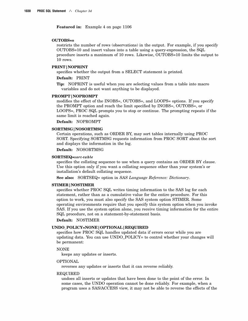
OUTOBS=nrestricts the number of rows (observations) in the output. For example, if you specifyOUTOBS=10 and insert values into a table using a query-expression, the SQLprocedure inserts a maximum of 10 rows. Likewise, OUTOBS=10 limits the output to10 rows.
PRINT|NOPRINTspecifies whether the output from a SELECT statement is printed.Default: PRINTTip: NOPRINT is useful when you are selecting values from a table into macro
variables and do not want anything to be displayed.
PROMPT|NOPROMPTmodifies the effect of the INOBS=, OUTOBS=, and LOOPS= options. If you specifythe PROMPT option and reach the limit specified by INOBS=, OUTOBS=, orLOOPS=, PROC SQL prompts you to stop or continue. The prompting repeats if thesame limit is reached again.Default: NOPROMPT
SORTMSG|NOSORTMSGCertain operations, such as ORDER BY, may sort tables internally using PROCSORT. Specifying SORTMSG requests information from PROC SORT about the sortand displays the information in the log.Default: NOSORTMSG
SORTSEQ=sort-tablespecifies the collating sequence to use when a query contains an ORDER BY clause.Use this option only if you want a collating sequence other than your system’s orinstallation’s default collating sequence.See also: SORTSEQ= option in SAS Language Reference: Dictionary.
STIMER|NOSTIMERspecifies whether PROC SQL writes timing information to the SAS log for eachstatement, rather than as a cumulative value for the entire procedure. For thisoption to work, you must also specify the SAS system option STIMER. Someoperating environments require that you specify this system option when you invokeSAS. If you use the system option alone, you receive timing information for the entireSQL procedure, not on a statement-by-statement basis.Default: NOSTIMER
UNDO_POLICY=NONE|OPTIONAL|REQUIREDspecifies how PROC SQL handles updated data if errors occur while you areupdating data. You can use UNDO_POLICY= to control whether your changes willbe permanent:
NONEkeeps any updates or inserts.
OPTIONALreverses any updates or inserts that it can reverse reliably.
REQUIREDundoes all inserts or updates that have been done to the point of the error. Insome cases, the UNDO operation cannot be done reliably. For example, when aprogram uses a SAS/ACCESS view, it may not be able to reverse the effects of the

The SQL Procedure 4 ALTER TABLE Statement 1031
INSERT and UPDATE statements without reversing the effects of other changesat the same time. In that case, PROC SQL issues an error message and does notexecute the statement. Also, when a SAS data set is accessed through a SAS/SHARE server and is opened with the data set option CNTLLEV=RECORD, youcannot reliably reverse your changes.
This option may enable other users to update newly inserted rows. If an erroroccurs during the insert, PROC SQL can delete a record that another user updated.In that case, the statement is not executed, and an error message is issued.
Default: REQUIREDNote: Options can be added, removed, or changed between PROC SQL statements
with the RESET statement. 4
ALTER TABLE Statement
Adds columns to, drops columns from, and changes column attributes in an existing table. Adds,modifies, and drops integrity constraints from an existing table.
Restriction: You cannot use any type of view in an ALTER TABLE statement.Restriction: You cannot use ALTER TABLE on a table that is accessed via an engine thatdoes not support UPDATE processing.Featured in: Example 3 on page 1104
ALTER TABLE table-name<constraint-clause> <, constraint-clause>...>;
<ADD column-definition <,column-definition>…><MODIFY column-definition
<,column-definition>…><DROP column <,column>…>;
where each constraint-clause is one of the following:
ADD <CONSTRAINT constraint-name> constraint
DROP CONSTRAINT constraint-name
DROP FOREIGN KEY constraint-name [Note: This is a DB2 extension.]
DROP PRIMARY KEY [Note: This is a DB2 extension.]
where constraint can be one of the following:
NOT NULL (column)
CHECK (WHERE-clause)
PRIMARY KEY (columns)
DISTINCT (columns)
UNIQUE (columns)
FOREIGN KEY (columns)REFERENCES table-name<ON DELETE referential-action > <ON UPDATE referential-action>

1032 ALTER TABLE Statement 4 Chapter 34
Arguments
columnnames a column in table-name.
column-definitionSee “column-definition” on page 1059.
constraint-namespecifies the name for the constraint being specified.
referential-actionspecifies the type of action to be performed on all matching foreign key values.
RESTRICToccurs only if there are matching foreign key values. This is the default referentialaction.
SET NULLsets all matching foreign key values to NULL.
table-namerefers to the name of table containing the primary key referenced by the foreign key.
WHERE-clausespecifies a SAS WHERE-clause.
Specifying Initial Values of New ColumnsWhen the ALTER TABLE statement adds a column to the table, it initializes the
column’s values to missing in all rows of the table. Use the UPDATE statement to addvalues to the new column(s).
Changing Column AttributesIf a column is already in the table, you can change the following column attributes
using the MODIFY clause: length, informat, format, and label. The values in a tableare either truncated or padded with blanks (if character data) as necessary to meet thespecified length attribute.
You cannot change a character column to numeric and vice versa. To change acolumn’s data type, drop the column and then add it (and its data) again, or use theDATA step.
Note: You cannot change the length of a numeric column with the ALTER TABLEstatement. Use the DATA step instead. 4
Renaming ColumnsTo change a column’s name, you must use the SAS data set option RENAME=. You
cannot change this attribute with the ALTER TABLE statement. RENAME= isdescribed in the section on SAS data set options in SAS Language Reference: Dictionary.
Indexes on Altered ColumnsWhen you alter the attributes of a column and an index has been defined for that
column, the values in the altered column continue to have the index defined for them.If you drop a column with the ALTER TABLE statement, all the indexes (simple and
The SQL Procedure 4 CREATE INDEX Statement 1033
composite) in which the column participates are also dropped. See “CREATE INDEXStatement” on page 1033 for more information on creating and using indexes.
Integrity ConstraintsUse ALTER TABLE to modify integrity constraints for existing tables. Use the
CREATE TABLE statement to attach integrity constraints to new tables. For moreinformation on integrity constraints, see the section on SAS files in SAS LanguageReference: Concepts.
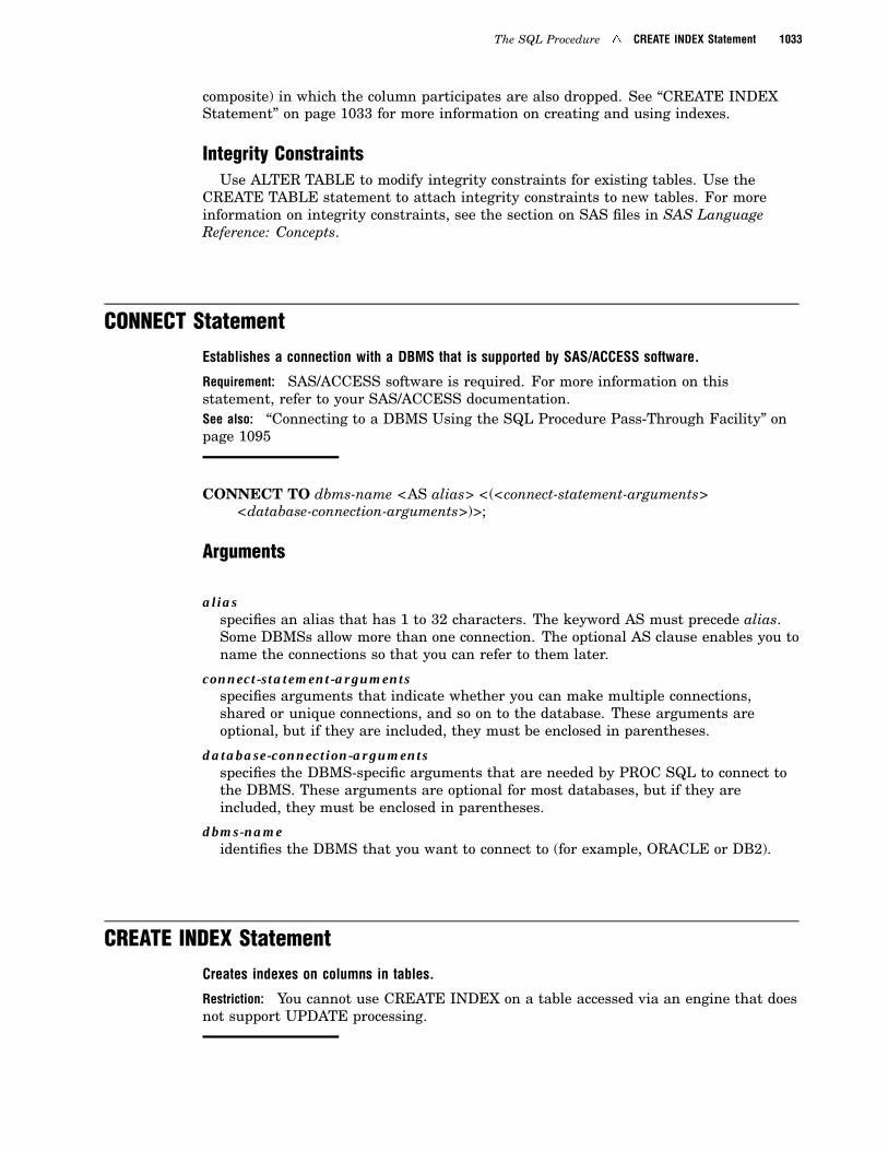
CONNECT StatementEstablishes a connection with a DBMS that is supported by SAS/ACCESS software.
Requirement: SAS/ACCESS software is required. For more information on thisstatement, refer to your SAS/ACCESS documentation.See also: “Connecting to a DBMS Using the SQL Procedure Pass-Through Facility” onpage 1095
CONNECT TO dbms-name <AS alias> <(<connect-statement-arguments><database-connection-arguments>)>;
Arguments
aliasspecifies an alias that has 1 to 32 characters. The keyword AS must precede alias.Some DBMSs allow more than one connection. The optional AS clause enables you toname the connections so that you can refer to them later.
connect-statement-argumentsspecifies arguments that indicate whether you can make multiple connections,shared or unique connections, and so on to the database. These arguments areoptional, but if they are included, they must be enclosed in parentheses.
database-connection-argumentsspecifies the DBMS-specific arguments that are needed by PROC SQL to connect tothe DBMS. These arguments are optional for most databases, but if they areincluded, they must be enclosed in parentheses.
dbms-nameidentifies the DBMS that you want to connect to (for example, ORACLE or DB2).
CREATE INDEX StatementCreates indexes on columns in tables.
Restriction: You cannot use CREATE INDEX on a table accessed via an engine that doesnot support UPDATE processing.

1034 CREATE INDEX Statement 4 Chapter 34
CREATE <UNIQUE> INDEX index-name
ON table-name (column <, column>…);
Arguments
columnspecifies a column in table-name.
index-namenames the index that you are creating. If you are creating an index on one columnonly, index-name must be the same as column. If you are creating an index on morethan one column, index-name cannot be the same as any column in the table.
table-namespecifies a PROC SQL table.
Indexes in PROC SQLAn index stores both the values of a table’s columns and a system of directions that
enable access to rows in that table by index value. Defining an index on a column or setof columns enables SAS, under certain circumstances, to locate rows in a table morequickly and efficiently. Indexes enable PROC SQL to execute the following classes ofqueries more efficiently:
� comparisons against a column that is indexed
� an IN subquery where the column in the inner subquery is indexed
� correlated subqueries, where the column being compared with the correlatedreference is indexed
� join-queries, where the join-expression is an equals comparison and all thecolumns in the join-expression are indexed in one of the tables being joined.
SAS maintains indexes for all changes to the table, whether the changes originatefrom PROC SQL or from some other source. Therefore, if you alter a column’s definitionor update its values, the same index continues to be defined for it. However, if anindexed column in a table is dropped, the index on it is also dropped.
You can create simple or composite indexes. A simple index is created on one columnin a table. A simple index must have the same name as that column. A composite indexis one index name that is defined for two or more columns. The columns can bespecified in any order, and they can have different data types. A composite index namecannot match the name of any column in the table. If you drop a composite index, theindex is dropped for all the columns named in that composite index.
UNIQUE KeywordThe UNIQUE keyword causes the SAS System to reject any change to a table that
would cause more than one row to have the same index value. Unique indexesguarantee that data in one column, or in a composite group of columns, remain uniquefor every row in a table. For this reason, a unique index cannot be defined for a columnthat includes NULL or missing values.
Managing IndexesYou can use the CONTENTS statement in the DATASETS procedure to display a
table’s index names and the columns for which they are defined. You can also use the

The SQL Procedure 4 CREATE TABLE Statement 1035
DICTIONARY tables INDEXES, TABLES, and COLUMNS to list information aboutindexes. See “DICTIONARY tables” on page 1062.
See the section on SAS files in SAS Language Reference: Dictionary for a furtherdescription of when to use indexes and how they affect SAS statements that handleBY-group processing.
CREATE TABLE Statement
Creates PROC SQL tables.
Featured in: Example 1 on page 1101 and Example 2 on page 1103
uCREATE TABLE table-name (column-definition <,column-definition>…);
(column-specification ,…<constraint-specification> ,…) ;
where column-specification is
column-definition <column-attribute>
where constraint-specification is
CONSTRAINT constraint-name constraint
column-attribute is one of the following:
UNIQUE
DISTINCT [Note: This is a DB2 extension. DISTINCT is the same as UNIQUE.]
NOT NULL
CHECK ( WHERE-clause )
PRIMARY KEY
REFERENCES table-name<ON DELETE referential-action > <ON UPDATE referential-action >
constraint is one of the following:
NOT NULL (column)
CHECK (WHERE-clause)
PRIMARY KEY (columns)
DISTINCT (columns)
UNIQUE (columns)
FOREIGN KEY (columns)REFERENCES table-name<ON DELETE referential-action> <ON UPDATE referential-action>
vCREATE TABLEtable-name LIKE table-name;
wCREATE TABLE table-name AS query-expression<ORDER BY order-by-item <,order-by-item>…>;

1036 CREATE TABLE Statement 4 Chapter 34
Arguments
column-definitionSee “column-definition” on page 1059.
constraint-nameis the name for the constraint being specified.
order-by-itemSee ORDER BY Clause on page 1053.
query-expressionSee “query-expression” on page 1075.
referential-actionspecifies the type of action to be performed on all matching foreign key values.
RESTRICToccurs only if there are matching foreign key values. This is the default referentialaction.
SET NULLsets all matching foreign key values to NULL.
table-nameis the name of the table containing the primary key referenced by the foreign key.
WHERE clausespecifies a SAS WHERE-clause.
Creating a Table without Rows
1 The first form of the CREATE TABLE statement creates tables that automaticallymap SQL data types to those supported by the SAS System. Use this form whenyou want to create a new table with columns that are not present in existingtables. It is also useful if you are running SQL statements from an SQLapplication in another SQL-based database.
2 The second form uses a LIKE clause to create a table that has the same columnnames and column attributes as another table. To drop any columns in the newtable, you can specify the DROP= data set option in the CREATE TABLEstatement. The specified columns are dropped when the table is created. Indexesare not copied to the new table.
Both of these forms create a table without rows. You can use an INSERTstatement to add rows. Use an ALTER statement to modify column attributes orto add or drop columns.
Creating a Table from a Query Expression
3 The third form of the CREATE TABLE statement stores the results of anyquery-expression in a table and does not display the output. It is a convenient wayto create temporary tables that are subsets or supersets of other tables.
When you use this form, a table is physically created as the statement isexecuted. The newly created table does not reflect subsequent changes in theunderlying tables (in the query-expression). If you want to continually access the

The SQL Procedure 4 CREATE VIEW Statement 1037
most current data, create a view from the query expression instead of a table. See“CREATE VIEW Statement” on page 1037.
Integrity ConstraintsYou can attach integrity constraints when you create a new table. To modify integrity
constraints, use the ALTER TABLE statement. For more information on integrityconstraints, see the section on SAS files in SAS Language Reference: Concepts.
CREATE VIEW Statement
Creates a PROC SQL view from a query-expression.
See also: “What Are Views?” on page 1023Featured in: Example 8 on page 1116
CREATE VIEW proc-sql-view AS query-expression<ORDER BY order-by-item <,order-by-item>…>
<USING statement<, libname-clause> ... > ;
where each libname-clause is one of the following:
LIBNAME libref <engine> ’SAS-data-library’ <option(s)> <engine-host-option(s)>
LIBNAME libref SAS/ACCESS-engine-name <SAS/ACCESS-engine-connection-option(s)> <SAS/ACCESS-engine-LIBNAME-option(s)>
Arguments
order-by-itemSee ORDER BY Clause on page 1053.
query-expressionSee “query-expression” on page 1075.
proc-sql-viewspecifies the name for the PROC SQL view that you are creating. See “What AreViews?” on page 1023 for a definition of a PROC SQL view.
Sorting Data Retrieved by ViewsPROC SQL allows you to specify the ORDER BY clause in the CREATE VIEW
statement. Every time a view is accessed, its data are sorted and displayed as specifiedby the ORDER BY clause. This sorting on every access has certain performance costs,especially if the view’s underlying tables are large. It is more efficient to omit theORDER BY clause when you are creating the view and specify it as needed when youreference the view in queries.
Note: If you specify the NUMBER option in the PROC SQL statement when youcreate your view, the ROW column appears in the output. However, you cannot order by

1038 CREATE VIEW Statement 4 Chapter 34
the ROW column in subsequent queries. See the description of the NUMBER option onpage 1030. 4
Librefs and Stored ViewsYou can refer to a table name alone (without the libref) in the FROM clause of a
CREATE VIEW statement if the table and view reside in the same SAS data library, asin this example:
create view proclib.view1 asselect *
from invoicewhere invqty>10;
In this view, VIEW1 and INVOICE are stored permanently in the SAS data libraryreferenced by PROCLIB. Specifying a libref for INVOICE is optional.
Updating ViewsYou can update a view’s underlying data with some restrictions. See “Updating
PROC SQL and SAS/ACCESS Views” on page 1097.
Embedded LIBNAME StatementsThe USING clause allows you to store DBMS connection information in a view by
embedding the SAS/ACCESS LIBNAME statement inside the view. When PROC SQLexecutes the view, the stored query assigns the libref and establishes the DBMSconnection using the information in the LIBNAME statement. The scope of the libref islocal to the view, and will not conflict with any identically named librefs in the SASsession. When the query finishes, the connection to the DBMS is terminated and thelibref is deassigned.
The USING clause must be the last clause in the SELECT statement. MultipleLIBNAME statements can be specified, separated by commas. In the following example,a connection is made and the libref ACCREC is assigned to an ORACLE database.
create view proclib.view1 asselect *
from accrec.invoices as invoicesusing libname accrec oracle
user=username pass=passwordpath=’dbms-path’;
For more information on the SAS/ACCESS LIBNAME statement, see the SAS/ACCESSdocumentation for your DBMS.
You can also embed a SAS LIBNAME statement in a view with the USING clause.This enables you to store SAS libref information in the view. Just as in the embeddedSAS/ACCESS LIBNAME statement, the scope of the libref is local to the view, and itwill not conflict with an identically named libref in the SAS session.
create view work.tableview asselect * from proclib.invoices
using libname proclib ’sas-data-library’;

The SQL Procedure 4 DESCRIBE Statement 1039
DELETE Statement
Removes one or more rows from a table or view that is specified in the FROM clause.
Restriction: You cannot use DELETE FROM on a table accessed via an engine that doesnot support UPDATE processing.Featured in: Example 5 on page 1108
DELETEFROM table-name|sas/access-view|proc-sql-view <AS alias>
<WHEREsql-expression>;
Arguments
aliasassigns an alias to table-name, sas/access-view, or proc-sql-view.
sas/access-viewspecifies a SAS/ACCESS view that you are deleting rows from.
proc-sql-viewspecifies a PROC SQL view that you are deleting rows from.
sql-expressionSee “sql-expression” on page 1081.
table-namespecifies the table that you are deleting rows from.
Deleting Rows Through ViewsYou can delete one or more rows from a view’s underlying table, with some
restrictions. See “Updating PROC SQL and SAS/ACCESS Views” on page 1097.
CAUTION:If you omit a WHERE clause, the DELETE statement deletes all the rows from the specifiedtable or the table described by a view. 4
DESCRIBE Statement
Displays a PROC SQL definition in the SAS log.
Restriction: PROC SQL views are the only type of view allowed in a DESCRIBE VIEWstatement.Featured in: Example 6 on page 1111
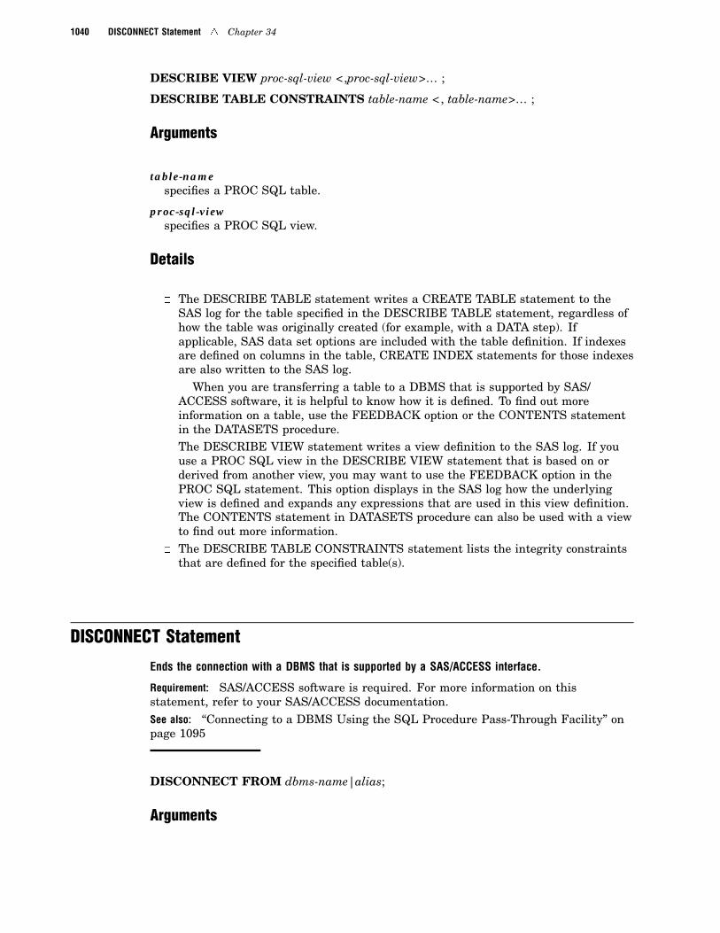
DESCRIBE TABLE table-name <,table-name>… ;
1040 DISCONNECT Statement 4 Chapter 34
DESCRIBE VIEW proc-sql-view <,proc-sql-view>… ;
DESCRIBE TABLE CONSTRAINTS table-name <, table-name>… ;
Arguments
table-namespecifies a PROC SQL table.
proc-sql-viewspecifies a PROC SQL view.
Details
� The DESCRIBE TABLE statement writes a CREATE TABLE statement to theSAS log for the table specified in the DESCRIBE TABLE statement, regardless ofhow the table was originally created (for example, with a DATA step). Ifapplicable, SAS data set options are included with the table definition. If indexesare defined on columns in the table, CREATE INDEX statements for those indexesare also written to the SAS log.
When you are transferring a table to a DBMS that is supported by SAS/ACCESS software, it is helpful to know how it is defined. To find out moreinformation on a table, use the FEEDBACK option or the CONTENTS statementin the DATASETS procedure.
� The DESCRIBE VIEW statement writes a view definition to the SAS log. If youuse a PROC SQL view in the DESCRIBE VIEW statement that is based on orderived from another view, you may want to use the FEEDBACK option in thePROC SQL statement. This option displays in the SAS log how the underlyingview is defined and expands any expressions that are used in this view definition.The CONTENTS statement in DATASETS procedure can also be used with a viewto find out more information.
� The DESCRIBE TABLE CONSTRAINTS statement lists the integrity constraintsthat are defined for the specified table(s).
DISCONNECT Statement
Ends the connection with a DBMS that is supported by a SAS/ACCESS interface.
Requirement: SAS/ACCESS software is required. For more information on thisstatement, refer to your SAS/ACCESS documentation.See also: “Connecting to a DBMS Using the SQL Procedure Pass-Through Facility” onpage 1095
DISCONNECT FROM dbms-name|alias;
Arguments

The SQL Procedure 4 DROP Statement 1041
aliasspecifies the alias that is defined in the CONNECT statement.
dbms-namespecifies the DBMS from which you want to end the connection (for example, DB2 orORACLE). The name you specify should match the name that is specified in theCONNECT statement.
Details
� An implicit COMMIT is performed before the DISCONNECT statement ends theDBMS connection. If a DISCONNECT statement is not submitted, implicitDISCONNECT and COMMIT actions are performed and the connection to theDBMS is broken when PROC SQL terminates.
� PROC SQL continues executing until you submit a QUIT statement, another SASprocedure, or a DATA step.
DROP Statement
Deletes tables, views, or indexes.
Restriction: You cannot use DROP TABLE or DROP INDEX on a table accessed via anengine that does not support UPDATE processing.
DROP TABLE table-name <,table-name>…;
DROP VIEW view-name <,view-name>…;
DROP INDEX index-name <,index-name>…FROM table-name;
Arguments
index-namespecifies an index that exists on table-name.
table-namespecifies a PROC SQL table.
view-namespecifies a SAS data view of any type: PROC SQL view, SAS/ACCESS view, or DATAstep view.
Details
� If you drop a table that is referenced in a view definition and try to execute theview, an error message is written to the SAS log stating that the table does not

1042 EXECUTE Statement 4 Chapter 34
exist. Therefore, remove references in queries and views to any table(s) andview(s) that you drop.
� If you drop a table with indexed columns, all the indexes are automaticallydropped. If you drop a composite index, the index is dropped for all the columnsthat are named in that index.
� You cannot use the DROP statement to drop a table or view in an externaldatabase that is described by a SAS/ACCESS view.
EXECUTE Statement
Sends a DBMS-specific SQL statement to a DBMS that is supported by a SAS/ACCESS interface.
Requirement: SAS/ACCESS software is required. For more information on thisstatement, refer to your SAS/ACCESS documentation.See also: “Connecting to a DBMS Using the SQL Procedure Pass-Through Facility” onpage 1095 and the SQL documentation for your DBMS.
EXECUTE (dbms-SQL-statement)BY dbms-name|alias;
Arguments
aliasspecifies an optional alias that is defined in the CONNECT statement. Note thatalias must be preceded by the keyword BY.
dbms-nameidentifies the DBMS to which you want to direct the DBMS statement (for example,ORACLE or DB2).
dbms-SQL-statementis any DBMS-specific SQL statement, except the SELECT statement, that can beexecuted by the DBMS-specific dynamic SQL.
Details
� If your DBMS supports multiple connections, you can use the alias that is definedin the CONNECT statement. This alias directs the EXECUTE statements to aspecific DBMS connection.
� Any return code or message that is generated by the DBMS is available in themacro variables SQLXRC and SQLXMSG after the statement completes.

The SQL Procedure 4 INSERT Statement 1043
INSERT Statement
Adds rows to a new or existing table or view.
Restriction: You cannot use INSERT INTO on a table accessed via an engine that doesnot support UPDATE processing.Featured in: Example 1 on page 1101
uINSERT INTOtable-name|sas/access-view|proc-sql-view<(column<,column>…)><,user-name>...;
SET column=sql-expression<,column=sql-expression>…<SET column=sql-expression<,column=sql-expression>…>;
vINSERT INTO table-name|sas/access-view|proc-sql-view <(column<,column>…)>VALUES (value <, value>…)
<VALUES (value <, value>…)>…;
wINSERT INTO table-name|sas/access-view|proc-sql-view<(column<,column>…)> query-expression;
Arguments
columnspecifies the column into which you are inserting rows.
sas/access-viewspecifies a SAS/ACCESS view into which you are inserting rows.
proc-sql-viewspecifies a PROC SQL view into which you are inserting rows.
sql-expressionSee “sql-expression” on page 1081.
table-namespecifies a PROC SQL table into which you are inserting rows.
valueis a data value.
Methods for Inserting Values
1 The first form of the INSERT statement uses the SET clause, which specifies oralters the values of a column. You can use more than one SET clause per INSERTstatement, and each SET clause can set the values in more than one column.Multiple SET clauses are not separated by commas. If you specify an optional listof columns, you can set a value only for a column that is specified in the list ofcolumns to be inserted.
2 The second form of the INSERT statement uses the VALUES clause. This clausecan be used to insert lists of values into a table. You can either give a value for
1044 RESET Statement 4 Chapter 34
each column in the table or give values just for the columns specified in the list ofcolumn names. One row is inserted for each VALUES clause. Multiple VALUESclauses are not separated by commas. The order of the values in the VALUESclause matches the order of the column names in the INSERT column list or, if nolist was specified, the order of the columns in the table.
3 The third form of the INSERT statement inserts the results of a query-expressioninto a table. The order of the values in the query-expression matches the order ofthe column names in the INSERT column list or, if no list was specified, the orderof the columns in the table.
Note: If the INSERT statement includes an optional list of column names, onlythose columns are given values by the statement. Columns that are in the table but notlisted are given missing values. 4
Inserting Rows through ViewsYou can insert one or more rows into a table through a view, with some restrictions.
See “Updating PROC SQL and SAS/ACCESS Views” on page 1097.
Adding Values to an Indexed ColumnIf an index is defined on a column and you insert a new row into the table, that value
is added to the index. You can display information about indexes with� the CONTENTS statement in the DATASETS procedure. See “CONTENTS
Statement” on page 346.� the DICTIONARY.INDEXES table. See “DICTIONARY tables” on page 1062 for
more information.
For more information on creating and using indexes, see “CREATE INDEXStatement” on page 1033.
RESET StatementResets PROC SQL options without restarting the procedure.
Featured in: Example 5 on page 1108
RESET <option(s)>;
The RESET statement enables you to add, drop, or change the options in PROC SQLwithout restarting the procedure. See “PROC SQL Statement” on page 1027 for adescription of the options.
SELECT StatementSelects columns and rows of data from tables and views.
See also: “table-expression” on page 1094, “query-expression” on page 1075

The SQL Procedure 4 SELECT Clause 1045
SELECT <DISTINCT> object-item <,object-item>…<INTO :macro-variable-specification
<, :macro-variable-specification>…>FROM from-list<WHERE sql-expression><GROUP BY group-by-item
<, group-by-item>…><HAVING sql-expression><ORDER BY order-by-item
<,order-by-item>…>;
SELECT Clause
Lists the columns that will appear in the output.
See Also: “column-definition” on page 1059Featured in: Example 1 on page 1101 and Example 2 on page 1103
SELECT <DISTINCT> object-item < ,object-item>…
� object-item is one of the following:
*
case-expression <AS alias>
column-name <AS alias><column-modifier <column-modifier>…>
sql-expression <AS alias><column-modifier <column-modifier>…>
table-name.*
table-alias.*
view-name.*
view-alias.*
Arguments
case-expressionSee “CASE expression” on page 1058.
column-modifierSee “column-modifier” on page 1060.
column-nameSee “column-name” on page 1061.
DISTINCTeliminates duplicate rows.

1046 INTO Clause 4 Chapter 34
Featured in: Example 13 on page 1126
sql-expressionSee “sql-expression” on page 1081.
table-aliasis an alias for a PROC SQL table.
table-namespecifies a PROC SQL table.
view-namespecifies any type of SAS data view.
view-aliasspecifies the alias for any type of SAS data view.
Asterisk(*) NotationThe asterisk (*) represents all columns of the table(s) listed in the FROM clause.
When an asterisk is not prefixed with a table name, all the columns from all tables inthe FROM clause are included; when it is prefixed (for example, table-name.* ortable-alias.*), all the columns from that table only are included.
Column AliasesA column alias is a temporary, alternate name for a column. Aliases are specified in
the SELECT clause to name or rename columns so that the result table is clearer oreasier to read. Aliases are often used to name a column that is the result of anarithmetic expression or summary function. An alias is one word only. If you need alonger column name, use the LABEL= column-modifier, as described in“column-modifier” on page 1060. The keyword AS is required with a column alias todistinguish the alias from other column names in the SELECT clause.
Column aliases are optional, and each column name in the SELECT clause can havean alias. After you assign an alias to a column, you can use the alias to refer to thatcolumn in other clauses.
If you use a column alias when creating a PROC SQL view, the alias becomes thepermanent name of the column for each execution of the view.
INTO Clause
Stores the value of one or more columns for use later in another PROC SQL query or SASstatement.
Restriction: An INTO clause cannot be used in a CREATE TABLE statement.See also: “Using Macro Variables Set by PROC SQL” on page 1096
INTO :macro-variable-specification<, :macro-variable-specification>…
� :macro-variable-specification is one of the following:
:macro-variable <SEPARATED BY ’character’ <NOTRIM>>;
The SQL Procedure 4 INTO Clause 1047
:macro-variable-1 − :macro-variable-n <NOTRIM>;
Arguments
macro-variablespecifies a SAS macro variable that stores the values of the rows that are returned.
NOTRIMprotects the leading and trailing blanks from being deleted from the macro variablevalue when the macro variables are created.
SEPARATED BY ’character’specifies a character that separates the values of the rows.
Details
� Use the INTO clause only in the outer query of a SELECT statement and not in asubquery.
� You can put multiple rows of the output into macro variables. You can check thePROC SQL macro variable SQLOBS to see the number of rows produced by aquery-expression. See “Using Macro Variables Set by PROC SQL” on page 1096 formore information on SQLOBS.
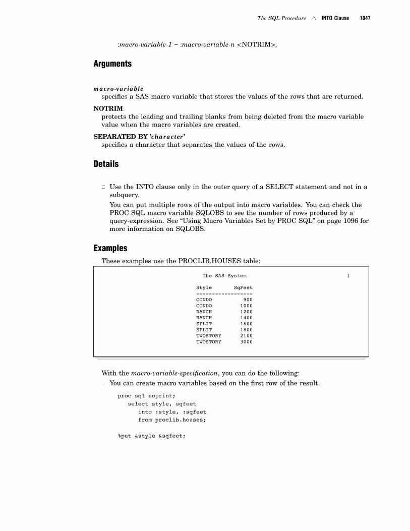
ExamplesThese examples use the PROCLIB.HOUSES table:
The SAS System 1
Style SqFeet------------------CONDO 900CONDO 1000RANCH 1200RANCH 1400SPLIT 1600SPLIT 1800TWOSTORY 2100TWOSTORY 3000
With the macro-variable-specification, you can do the following:� You can create macro variables based on the first row of the result.
proc sql noprint;select style, sqfeet
into :style, :sqfeetfrom proclib.houses;
%put &style &sqfeet;

1048 INTO Clause 4 Chapter 34
The results are written to the SAS log:
1 proc sql noprint;2 select style, sqfeet3 into :style, :sqfeet4 from proclib.houses;56 %put &style &sqfeet;CONDO 900
� You can create one new macro variable per row in the result of the SELECTstatement. This example shows how you can request more values for one columnthan for another. The hyphen (-) is used in the INTO clause to imply a range ofmacro variables. You can use either the keywords THROUGH or THRU instead ofa hyphen.
The following PROC SQL step puts the values from the first four rows of thePROCLIB.HOUSES table into macro variables:
proc sql noprint;select distinct Style, SqFeet
into :style1 - :style3, :sqfeet1 - :sqfeet4from proclib.houses;
%put &style1 &sqfeet1;%put &style2 &sqfeet2;%put &style3 &sqfeet3;%put &sqfeet4;
The %PUT statements write the results to the SAS log:
1 proc sql noprint;2 select distinct style, sqfeet3 into :style1 - :style3, :sqfeet1 - :sqfeet44 from proclib.houses;56 %put &style1 &sqfeet1;CONDO 9007 %put &style2 &sqfeet2;CONDO 10008 %put &style3 &sqfeet3;CONDO 12009 %put &sqfeet4;1400
� You can concatenate the values of one column into one macro variable. This formis useful for building up a list of variables or constants.
proc sql;select distinct style
into :s1 separated by ’,’from proclib.houses;
%put &s1;

The SQL Procedure 4 FROM Clause 1049
The results are written to the SAS log:
3 proc sql;4 select distinct style5 into :s1 separated by ’,’6 from proclib.houses;78 %put &s1
CONDO,RANCH,SPLIT,TWOSTORY
� The leading and trailing blanks are trimmed from the values before the macrovariables are created. If you do not want the blanks to be trimmed, add NOTRIM,as shown in the following example:
proc sql noprint;select style, sqfeet
into :style1 - :style4 notrim,:sqfeet separated by ’,’ notrim
from proclib.houses;
%put *&style1* *&sqfeet*;%put *&style2* *&sqfeet*;%put *&style3* *&sqfeet*;%put *&style4* *&sqfeet*;
The results are written to the SAS log, as shown in Output 34.1 on page 1049.
Output 34.1 Macro Variable Values
3 proc sql noprint;4 select style, sqfeet5 into :style1 - :style4 notrim,6 :sqfeet separated by ’,’ notrim7 from proclib.houses;89 %put *&style1* *&sqfeet*;*CONDO * * 900, 1000, 1200, 1400, 1600, 1800, 2100,
3000*10 %put *&style2* *&sqfeet*;*CONDO * * 900, 1000, 1200, 1400, 1600, 1800, 2100,
3000*11 %put *&style3* *&sqfeet*;*RANCH * * 900, 1000, 1200, 1400, 1600, 1800, 2100,
3000*12 %put *&style4* *&sqfeet*;*RANCH * * 900, 1000, 1200, 1400, 1600, 1800, 2100,
3000*
FROM Clause
Specifies source tables or views.
Featured in: Example 1 on page 1101, Example 4 on page 1106, Example 9 on page 1118,and Example 10 on page 1121
FROM from-list

1050 FROM Clause 4 Chapter 34
� from-list is one of the following:
table-name <<AS> alias>
view-name <<AS> alias>
joined-table
(query-expression) <<AS> alias<(column < ,column>…)>>
CONNECTION TO
Arguments
columnnames the column that appears in the output. The column names that you specifyare matched by position to the columns in the output.
CONNECTION TOSee “CONNECTION TO” on page 1062.
joined-tableSee “joined-table” on page 1068.
query-expressionSee “query-expression” on page 1075.
table-namespecifies a PROC SQL table.
view-namespecifies any type of SAS data view.
Table AliasesA table alias is a temporary, alternate name for a table that is specified in the FROM
clause. Table aliases are prefixed to column names to distinguish between columns thatare common to multiple tables. Table aliases are always required when joining a tablewith itself. Column names in other kinds of joins must be prefixed with table aliases ortable names unless the column names are unique to those tables.
The optional keyword AS is often used to distinguish a table alias from other tablenames.
In-Line ViewsThe FROM clause can itself contain a query-expression that takes an optional table
alias. This kind of nested query-expression is called an in-line view. An in-line view isany query-expression that would be valid in a CREATE VIEW statement. PROC SQLcan support many levels of nesting, but it is limited to 32 tables in any one query. The32–table limit includes underlying tables that may contribute to views that arespecified in the FROM clause.
An in-line view saves you a programming step. Rather than creating a view andreferring to it in another query, you can specify the view in-line in the FROM clause.
Characteristics of in-line views include the following:� An in-line view is not assigned a permanent name, although it can take an alias.
The SQL Procedure 4 WHERE Clause 1051
� An in-line view can be referred to only in the query in which it is defined. Itcannot be referenced in another query.
� You cannot use an ORDER BY clause in an in-line view.
� The names of columns in an in-line view can be assigned in the object-item list ofthat view or with a parenthesized list of names following the alias. This syntaxcan be useful for renaming columns. See Example 10 on page 1121 for an example.
WHERE Clause
Subsets the output based on specified conditions.
Featured in: Example 4 on page 1106 and Example 9 on page 1118
WHERE sql-expression
Argument
sql-expressionSee “sql-expression” on page 1081.
Details
� When a condition is met (that is, the condition resolves to true), those rows aredisplayed in the result table; otherwise, no rows are displayed.
� You cannot use summary functions that specify only one column. For example:
where max(measure1) > 50;
However, this WHERE clause will work:
where max(measure1,measure2) > 50;
Writing Efficient WHERE ClausesHere are some guidelines for writing efficient WHERE clauses that enable PROC
SQL to use indexes effectively:
� Avoid using LIKE predicates that begin with % or _:
/* inefficient:*/ where country like ’%INA’/* efficient: */ where country like ’A%INA’
� Avoid using arithmetic expressions in a predicate:
/* inefficient:*/ where salary>12*4000/* efficient: */ where salary>48000
� First put the expression that returns the fewest number of rows. In the followingquery, there are fewer rows where miles>3800 than there are where boarded>100.
where miles>3800 and boarded>100

1052 GROUP BY Clause 4 Chapter 34
GROUP BY Clause
Specifies how to group the data for summarizing.
Featured in: Example 8 on page 1116 and Example 12 on page 1124
GROUP BY group-by-item < ,group-by-item>…
� group-by-item is one of the following:
integer
column-name
sql-expression
Arguments
integerequates to a column’s position.
column-nameSee “column-name” on page 1061.
sql-expressionSee “sql-expression” on page 1081.
Details
� You can specify more than one group-by-item to get more detailed reports. Boththe grouping of multiple items and the BY statement of a PROC step areevaluated in similiar ways. If more than one group-by-item is specified, the firstone determines the major grouping.
� Integers can be substituted for column names (that is, SELECT object-items) inthe GROUP BY clause. For example, if the group-by-item is 2, the results aregrouped by the values in the second column of the SELECT clause list. Usingintegers can shorten your coding and enable you to group by the value of anunnamed expression in the SELECT list.
� The data do not have to be sorted in the order of the group-by values becausePROC SQL handles sorting automatically. You can use the ORDER BY clause tospecify the order in which rows are displayed in the result table.
� If you specify a GROUP BY clause in a query that does not contain a summaryfunction, your clause is transformed into an ORDER BY clause and a message tothat effect is written to the SAS log.
� A group-by-item cannot be a summary function. For example, the followingGROUP BY clause is not valid:
group by sum(x)

The SQL Procedure 4 ORDER BY Clause 1053
HAVING Clause
Subsets grouped data based on specified conditions.
Featured in: Example 8 on page 1116 and Example 12 on page 1124
HAVING sql-expression
Argument
sql-expressionSee “sql-expression” on page 1081.
Subsetting Grouped DataThe HAVING clause is used with at least one summary function and an optional
GROUP BY clause to summarize groups of data in a table. A HAVING clause is anyvalid SQL expression that is evaluated as either true or false for each group in a query.Or, if the query involves remerged data, the HAVING expression is evaluated for eachrow that participates in each group. The query must include one or more summaryfunctions.
Typically, the GROUP BY clause is used with the HAVING expression and definesthe group(s) to be evaluated. If you omit the GROUP BY clause, the summary functionand the HAVING clause treat the table as one group.
The following PROC SQL step uses the PROCLIB.PAYROLL table (shown inExample 2 on page 1103) and groups the rows by SEX to determine the oldest employeeof each sex. In SAS, dates are stored as integers. The lower the birthdate as an integer,the greater the age. The expression birth=min(birth)is evaluated for each row in thetable. When the minimum birthdate is found, the expression becomes true and the rowis included in the output.
proc sql;title ’Oldest Employee of Each Gender’;select *
from proclib.payrollgroup by sexhaving birth=min(birth);
Note: This query involves remerged data because the values returned by asummary function are compared to values of a column that is not in the GROUP BYclause. See “Remerging Data” on page 1090 for more information about summaryfunctions and remerging data. 4
ORDER BY Clause
Specifies the order in which rows are displayed in a result table.
See also: “query-expression” on page 1075Featured in: Example 11 on page 1122

1054 ORDER BY Clause 4 Chapter 34
ORDER BY order-by-item < ,order-by-item>…;
� order-by-item is one of the following:
integer <ASC|DESC>
column-name <ASC|DESC>
sql-expression <ASC|DESC>
Arguments
ASCorders the data in ascending order. This is the default order.
column-nameSee “column-name” on page 1061.
DESCorders the data in descending order.
integerequates to a column’s position.
sql-expressionSee “sql-expression” on page 1081.
Details
� The ORDER BY clause sorts the result of a query expression according to theorder specified in that query. When this clause is used, the default orderingsequence is ascending, from the lowest value to the highest. You can use theSORTSEQ= option to change the collating sequence for your output. See “PROCSQL Statement” on page 1027.
� If an ORDER BY clause is omitted, the SAS System’s default collating sequenceand your operating environment determine the order of a result table’s rows.Therefore, if you want your result table to appear in a particular order, use theORDER BY clause.
� Using an ORDER BY clause has certain performance costs, as does any sortingprocedure. If you are querying large tables, and the order of their results is notimportant, your queries will run faster without an ORDER BY clause.
� If more than one order-by-item is specified (separated by commas), the first onedetermines the major sort order. For example, if the order-by-item is 2 (an integer),the results are ordered by the values of the second column. If a query-expressionincludes a set operator (for example, UNION), use integers to specify the order.Doing so avoids ambiguous references to columns in the table expressions.
� In the ORDER BY clause, you can specify any column of a table or view that isspecified in the FROM clause of a query-expression, regardless of whether thatcolumn has been included in the query’s SELECT clause. For example, this queryproduces a report ordered by the descending values of the population change foreach country from 1990 to 1995:
proc sql;select country

The SQL Procedure 4 UPDATE Statement 1055
from censusorder by pop95-pop90 desc;
NOTE: The query as specified involvesordering by an item thatdoesn’t appear in its SELECT clause.
� You can order the output by the values that are returned by a function, forexample:
proc sql;select *
from measureorder by put(pol_a,fmt_a.);
UPDATE Statement
Modifies a column’s values in existing rows of a table or view.
Restriction: You cannot use UPDATE on a table accessed via an engine that does notsupport UPDATE processing.
Featured in: Example 3 on page 1104
UPDATE table-name|sas/access-view|proc-sql-view <AS alias>
SET column=sql-expression<,column=sql-expression>…
<SETcolumn=sql-expression<,column=sql-expression>…>
<WHEREsql-expression>;
Arguments
aliasassigns an alias to table-name, sas/access-view, or proc-sql-view.
columnspecifies a column in table-name, sas/access-view, or proc-sql-view.
sas/access-viewspecifies a SAS/ACCESS view.
sql-expressionSee “sql-expression” on page 1081.
table-namespecifies a PROC SQL table.
proc-sql-viewspecifies a PROC SQL view.
1056 VALIDATE Statement 4 Chapter 34
Updating Tables through ViewsYou can update one or more rows of a table through a view, with some restrictions.
See “Updating PROC SQL and SAS/ACCESS Views” on page 1097.
Details
� Any column that is not modified retains its original values, except in certainqueries using the CASE expression. See “CASE expression” on page 1058 for adescription of CASE expressions.
� To add, drop, or modify a column’s definition or attributes, use the ALTER TABLEstatement, described in “ALTER TABLE Statement” on page 1031.
� In the SET clause, a column reference on the left side of the equal sign can alsoappear as part of the expression on the right side of the equal sign. For example,you could use this expression to give employees a $1,000 holiday bonus:
set salary=salary + 1000
� If you omit the WHERE clause, all the rows are updated. When you use aWHERE clause, only the rows that meet the WHERE condition are updated.
� When you update a column and an index has been defined for that column, thevalues in the updated column continue to have the index defined for them.
VALIDATE StatementChecks the accuracy of a query-expression’s syntax without executing the expression.
VALIDATE query-expression;
Argument
query-expressionSee “query-expression” on page 1075.
Details
� The VALIDATE statement writes a message in the SAS log that states that thequery is valid. If there are errors, VALIDATE writes error messages to the SAS log.
� The VALIDATE statement can also be included in applications that use the macrofacility. When used in such an application, VALIDATE returns a value thatindicates the query-expression’s validity. The value is returned through the macrovariable SQLRC (a short form for SQL return code). For example, if a SELECTstatement is valid, the macro variable SQLRC returns a value of 0. See “UsingMacro Variables Set by PROC SQL” on page 1096 for more information.
Component DictionaryThis section describes the components that are used in SQL procedure statements.
Components are the items in PROC SQL syntax that appear in roman type.

The SQL Procedure 4 CALCULATED 1057
Most components are contained in clauses within the statements. For example, thebasic SELECT statement is composed of the SELECT and FROM clauses, where eachclause contains one or more components. Components can also contain othercomponents.
For easy reference, components appear in alphabetical order, and some terms arereferred to before they are defined. Use the index or the "See Also" references to referto other statement or component descriptions that may be helpful.
BETWEEN condition
Selects rows where column values are within a range of values.
sql-expression <NOT> BETWEEN sql-expressionAND sql-expression
� sql-expression is described in “sql-expression” on page 1081.
Details
� The sql-expressions must be of compatible data types. They must be either allnumeric or all character types.
� Because a BETWEEN condition evaluates the boundary values as a range, it isnot necessary to specify the smaller quantity first.
� You can use the NOT logical operator to exclude a range of numbers, for example,to eliminate customer numbers between 1 and 15 (inclusive) so that you canretrieve data on more recently acquired customers.
� PROC SQL supports the same comparison operators that the DATA step supports.For example:
x between 1 and 3x between 3 and 11<=x<=3x>=1 and x<=3
CALCULATED
Refers to columns already calculated in the SELECT clause.
CALCULATED column-alias
� column-alias is the name assigned to the column in the SELECT clause.
1058 CASE expression 4 Chapter 34
Referencing a CALCULATED ColumnCALCULATED enables you to use the results of an expression in the same SELECT
clause or in the WHERE clause. It is valid only when used to refer to columns that arecalculated in the immediate query expression.
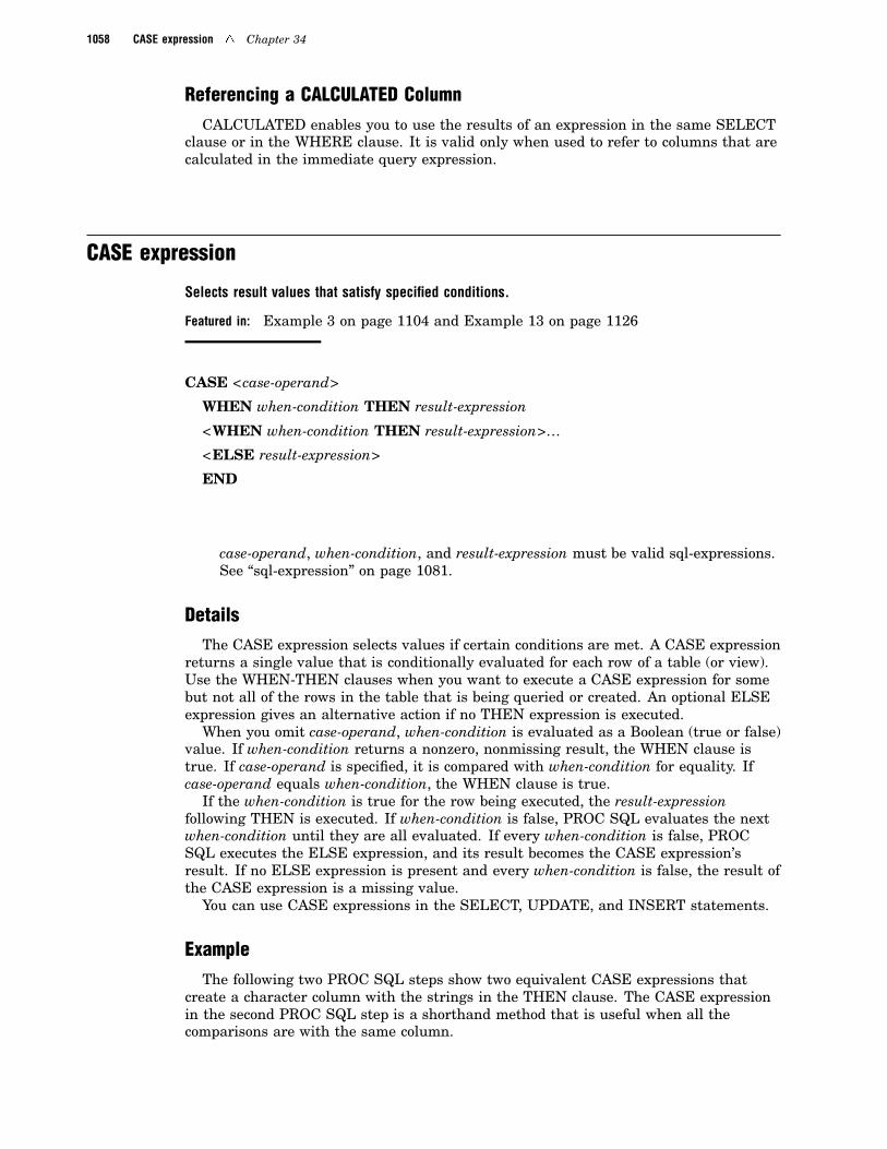
CASE expression
Selects result values that satisfy specified conditions.
Featured in: Example 3 on page 1104 and Example 13 on page 1126
CASE <case-operand>
WHEN when-condition THEN result-expression
<WHEN when-condition THEN result-expression>…
<ELSE result-expression>
END
� case-operand, when-condition, and result-expression must be valid sql-expressions.See “sql-expression” on page 1081.
DetailsThe CASE expression selects values if certain conditions are met. A CASE expression
returns a single value that is conditionally evaluated for each row of a table (or view).Use the WHEN-THEN clauses when you want to execute a CASE expression for somebut not all of the rows in the table that is being queried or created. An optional ELSEexpression gives an alternative action if no THEN expression is executed.
When you omit case-operand, when-condition is evaluated as a Boolean (true or false)value. If when-condition returns a nonzero, nonmissing result, the WHEN clause istrue. If case-operand is specified, it is compared with when-condition for equality. Ifcase-operand equals when-condition, the WHEN clause is true.
If the when-condition is true for the row being executed, the result-expressionfollowing THEN is executed. If when-condition is false, PROC SQL evaluates the nextwhen-condition until they are all evaluated. If every when-condition is false, PROCSQL executes the ELSE expression, and its result becomes the CASE expression’sresult. If no ELSE expression is present and every when-condition is false, the result ofthe CASE expression is a missing value.
You can use CASE expressions in the SELECT, UPDATE, and INSERT statements.
ExampleThe following two PROC SQL steps show two equivalent CASE expressions that
create a character column with the strings in the THEN clause. The CASE expressionin the second PROC SQL step is a shorthand method that is useful when all thecomparisons are with the same column.

The SQL Procedure 4 column-definition 1059
Example Code 34.1
proc sql;select *, case
when degrees > 80 then ’Hot’when degrees < 40 then ’Cold’else ’Mild’end
from temperatures;
proc sql;select *, case Degrees
when > 80 then ’Hot’when < 40 then ’Cold’else ’Mild’end
from temperatures;
column-definition
Defines PROC SQL’s data types and dates.
See also: “column-modifier” on page 1060Featured in: Example 1 on page 1101
column CHARACTER|VARCHAR <(width)><column-modifier <column-modifier>…>
column INTEGER|SMALLINT<column-modifier <column-modifier>…>
column DECIMAL|NUMERIC|FLOAT <(width< ,ndec>)><column-modifier <column-modifier>…>
column REAL|DOUBLE PRECISION<column-modifier <column-modifier>…>
column DATE <column-modifier>
� column-modifier is described in “column-modifier” on page 1060.� ndec is the number of decimals. PROC SQL ignores ndec. It is included for
compatibility with SQL from other software.� width is the width of the column. The width field on a character column specifies
the width of that column; it defaults to eight characters. PROC SQL ignores awidth field on a numeric column. All numeric columns are created with themaximum precision allowed by the SAS System. If you want to create numericcolumns that use less storage space, use the LENGTH statement in the DATA step.
Details

1060 column-modifier 4 Chapter 34
� SAS supports many but not all of the data types that SQL-based databasessupport. The SQL procedure defaults to the SAS data types NUM and CHAR.
� The CHARACTER, INTEGER, and DECIMAL data types can be abbreviated toCHAR, INT, and DEC, respectively.
� A column declared with DATE is a SAS numeric variable with a date informat orformat. You can use any of the column-modifiers to set the appropriate attributesfor the column being defined. See SAS Language Reference: Dictionary for moreinformation on dates.
column-modifier
Sets column attributes.
See also: “column-definition” on page 1059 and SELECT Clause on page 1045Featured in: Example 1 on page 1101 and Example 2 on page 1103
<INFORMAT=informatw.d>
<FORMAT=formatw.d>
<LABEL=’label’>
<LENGTH=length>
Specifying Informats for Columns (INFORMAT=)INFORMAT= specifies the informat to be used when SAS accesses data from a table
or view. You can change one permanent informat to another by using the ALTERstatement. PROC SQL stores informats in its table definitions so that other SASprocedures and the DATA step can use this information when they reference tablescreated by PROC SQL.
Specifying Formats for Columns (FORMAT=)FORMAT= determines how character and numeric values in a column are displayed
by the query-expression. If the FORMAT= modifier is used in the ALTER, CREATETABLE, or CREATE VIEW statements, it specifies the permanent format to be usedwhen SAS displays data from that table or view. You can change one permanent formatto another by using the ALTER statement.
See SAS Language Reference: Dictionary for more information on informats andformats.
Specifying Labels for Columns (LABEL=)LABEL= associates a label with a column heading. If the LABEL= modifier is used
in the ALTER, CREATE TABLE, or CREATE VIEW statements, it specifies thepermanent label to be used when displaying that column. You can change onepermanent label to another by using the ALTER statement.
If you refer to a labeled column in the ORDER BY or GROUP BY clause, you mustuse either the column name (not its label), the column’s alias, or its ordering integer

The SQL Procedure 4 column-name 1061
(for example, ORDER BY 2). See the section on SAS statements in SAS LanguageReference: Dictionary for more information on labels.
A label can begin with the following characters: a through z, A through Z, 0 through9, an underscore (_), or a blank space. If you begin a label with any other character,such as pound sign (#), that character is used as a split character and it splits the labelonto the next line wherever it appears. For example:
select dropout label=’#Percentage of#Students Who#Dropped Out’
from educ(obs=5);
If you need a special character to appear as the first character in the output, precedeit with a space or a forward slash (/).
You can omit the LABEL= part of the column-modifier and still specify a label. Besure to enclose the label in quotes. For example:
select empname "Names of Employees"from sql.employees;
If you need an apostrophe in the label, type it twice so that the SAS System readsthe apostrophe as a literal. Or, you can use single and double quotes alternately (forexample, “Date Rec’d”).
column-name
Specifies the column to select.
See also: “column-modifier” on page 1060 and SELECT Clause on page 1045
column-name is one of the following:
column
table-name.column
table-alias.column
view-name.column
view-alias.column
Qualifying Column NamesA column can be referred to by its name alone if it is the only column by that name
in all the tables or views listed in the current query-expression. If the same columnname exists in more than one table or view in the query expression, you must qualifyeach use of the column name by prefixing a reference to the table that contains it.Consider the following examples:
SALARY /* name of the column */EMP.SALARY /* EMP is the table or view name */E.SALARY /* E is an alias for the table
or view that contains theSALARY column */

1062 CONNECTION TO 4 Chapter 34
CONNECTION TO
Retrieves and uses DBMS data in a PROC SQL query or view.
Tip: You can use CONNECTION TO in the SELECT statement’s FROM clause as partof the from-list.See also: “Connecting to a DBMS Using the SQL Procedure Pass-Through Facility” onpage 1095 and your SAS/ACCESS documentation.
CONNECTION TO dbms-name (dbms-query)
CONNECTION TO alias (dbms-query)
� alias specifies an alias, if one was defined in the CONNECT statement.� dbms-name identifies the DBMS you are using.� dbms-query specifies the query to send to a DBMS. The query uses the DBMS’s
dynamic SQL. You can use any SQL syntax that the DBMS understands, even ifthat is not valid for PROC SQL. However, your DBMS query cannot contain asemicolon because that represents the end of a statement to the SAS System.
The number of tables that you can join with dbms-query is determined by theDBMS. Each CONNECTION TO component counts as one table toward the32-table PROC SQL limit for joins.
CONTAINS condition
Tests whether a string is part of a column’s value.
Restriction: The CONTAINS condition is used only with character operands.Featured in: Example 7 on page 1112
sql-expression<NOT> CONTAINS sql-expression
For more information, see “sql-expression” on page 1081.
DICTIONARY tables
Retrieve information about elements associated with the current SAS session.
Restriction: You cannot use SAS data set options with DICTIONARY tables.Restriction: DICTIONARY tables are read-only objects.
Featured in: Example 6 on page 1111

The SQL Procedure 4 DICTIONARY tables 1063
DICTIONARY. table-name
� table-name is one of the following:
CATALOGS MEMBERS
COLUMNS OPTIONS
EXTFILES TABLES
INDEXES TITLES
MACROS VIEWS
Querying DICTIONARY Tables
The DICTIONARY tables component is specified in the FROM clause of a SELECTstatement. DICTIONARY is a reserved libref for use only in PROC SQL. Data fromDICTIONARY tables are generated at run time.
You can use a PROC SQL query to retrieve or subset data from a DICTIONARYtable. You can save that query as a PROC SQL view for use later. Or, you can use theexisting SASHELP views that are created from the DICTIONARY tables.
To see how each DICTIONARY table is defined, submit a DESCRIBE TABLEstatement. After you know how a table is defined, you can use its column names in asubsetting WHERE clause to get more specific information. For example:
proc sql;describe table dictionary.indexes;
The results are written to the SAS log:
1 proc sql;2 describe table dictionary.indexes;NOTE: SQL table DICTIONARY.INDEXES was created like:
create table DICTIONARY.INDEXES(
libname char(8) label=’Library Name’,memname char(32) label=’Member Name’,memtype char(8) label=’Member Type’,name char(32) label=’Column Name’,idxusage char(9) label=’Column Index Type’,indxname char(32) label=’Index Name’,indxpos num label=’Position of Column in Concatenated Key’,nomiss char(3) label=’Nomiss Option’,unique char(3) label=’Unique Option’
);
You specify a DICTIONARY table in a PROC SQL query or view to retrieveinformation about its objects. For example, the following query returns a row for eachindex in the INDEXES DICTIONARY table:
proc sql;title ’DICTIONARY.INDEXES Table’;select * from dictionary.indexes;

1064 DICTIONARY tables 4 Chapter 34
Subsetting Data from DICTIONARY Tables
DICTIONARY tables are often large. Therefore, if you are looking for specificinformation, use a WHERE clause to retrieve a subset of the rows in a DICTIONARYtable. In the following example, only the rows with the member name ADBDBI aredisplayed from the DICTIONARY.CATALOGS table:
proc sql ;title ’Subset of the DICTIONARY.CATALOGS Table’;title2 ’Rows with Member Name ADBDBI ’;
select * from dictionary.catalogswhere memname =’ADBDBI’;
Creating PROC SQL Views from DICTIONARY Tables
To use DICTIONARY tables in other SAS procedures or in the DATA step, use PROCSQL views that are based on the DICTIONARY tables.
You can either create a PROC SQL view on a DICTIONARY table or you can use theSASHELP views, as described in “Accessing DICTIONARY Tables with SASHELPViews” on page 1065. You can then use the view in a DATA or PROC step. Thefollowing example creates a PROC SQL view on the DICTIONARY.OPTIONS table.Output 34.2 on page 1064 displays the view with PROC PRINT:
options linesize=120 nodate pageno=1;
proc sql;create view work.options as
select * from dictionary.options;
proc print data=work.options(obs=10) noobs;title ’Listing of the View WORK.OPTIONS’;title2 ’First 10 Rows Only’;
run;
Output 34.2 DICTIONARY.OPTIONS Table (partial output)
Listing of the View WORK.OPTIONS 1
First 10 Rows Only
optname setting optdesc level
BATCH NOBATCH Use the batch set of default values for SAS system options Portable
BINDING DEFAULT Controls the binding edge for duplexed output Portable
BOTTOMMARGIN Bottom margin for printed output Portable
BUFNO 1 Number of buffers for each SAS data set Portable
BUFSIZE 0 Size of buffer for page of SAS data set Portable
BYERR BYERR Set the error flag if a null data set is input to the SORT procedure Portable
BYLINE BYLINE Print the by-line at the beginning of each by-group Portable
CAPS NOCAPS Translate SAS source and data lines to uppercase Portable
CARDIMAGE NOCARDIMAGE Process SAS source and data lines as 80-byte records Portable
CATCACHE 0 Number of SAS catalogs to keep in cache memory Portable
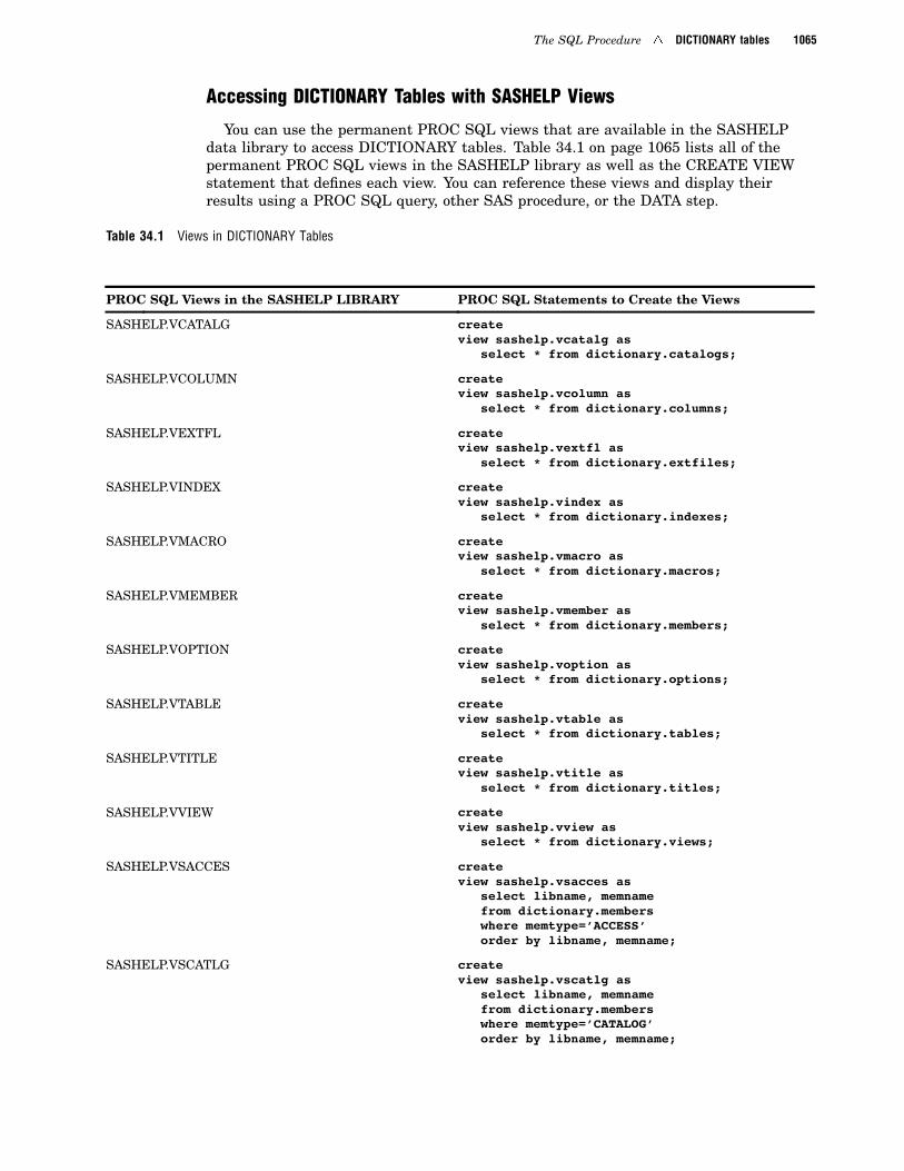
The SQL Procedure 4 DICTIONARY tables 1065
Accessing DICTIONARY Tables with SASHELP Views
You can use the permanent PROC SQL views that are available in the SASHELPdata library to access DICTIONARY tables. Table 34.1 on page 1065 lists all of thepermanent PROC SQL views in the SASHELP library as well as the CREATE VIEWstatement that defines each view. You can reference these views and display theirresults using a PROC SQL query, other SAS procedure, or the DATA step.
Table 34.1 Views in DICTIONARY Tables
PROC SQL Views in the SASHELP LIBRARY PROC SQL Statements to Create the Views
SASHELP.VCATALG createview sashelp.vcatalg as
select * from dictionary.catalogs;
SASHELP.VCOLUMN createview sashelp.vcolumn as
select * from dictionary.columns;
SASHELP.VEXTFL createview sashelp.vextfl as
select * from dictionary.extfiles;
SASHELP.VINDEX createview sashelp.vindex as
select * from dictionary.indexes;
SASHELP.VMACRO createview sashelp.vmacro as
select * from dictionary.macros;
SASHELP.VMEMBER createview sashelp.vmember as
select * from dictionary.members;
SASHELP.VOPTION createview sashelp.voption as
select * from dictionary.options;
SASHELP.VTABLE createview sashelp.vtable as
select * from dictionary.tables;
SASHELP.VTITLE createview sashelp.vtitle as
select * from dictionary.titles;
SASHELP.VVIEW createview sashelp.vview as
select * from dictionary.views;
SASHELP.VSACCES createview sashelp.vsacces as
select libname, memnamefrom dictionary.memberswhere memtype=’ACCESS’order by libname, memname;
SASHELP.VSCATLG createview sashelp.vscatlg as
select libname, memnamefrom dictionary.memberswhere memtype=’CATALOG’order by libname, memname;

1066 EXISTS condition 4 Chapter 34
PROC SQL Views in the SASHELP LIBRARY PROC SQL Statements to Create the Views
SASHELP.VSLIB create
view sashelp.vslib asselect distinct libname, pathfrom dictionary.membersorder by libname;
SASHELP.VSTABLE createview sashelp.vstable as
select libname, memnamefrom dictionary.memberswhere memtype=’DATA’order by libname, memname;
SASHELP.VSTABVW createview sashelp.vstabvw as
select libname, memname, memtypefrom dictionary.memberswhere memtype=’VIEW’ or memtype=’DATA’order by libname, memname;
SASHELP.VSVIEW createview sashelp.vsview as
select libname, memnamefrom dictionary.memberswhere memtype=’VIEW’order by libname, memname;
EXISTS condition
Tests if a subquery returns one or more rows.
See also: “Query Expressions (Subqueries)” on page 1083
<NOT> EXISTS (query-expression)
� query-expression is described in “query-expression” on page 1075.
DetailsThe EXISTS condition is an operator whose right operand is a subquery. The result
of an EXISTS condition is true if the subquery resolves to at least one row. The resultof a NOT EXISTS condition is true if the subquery evaluates to zero rows. For example,the following query subsets PROCLIB.PAYROLL (which is shown in Example 2 on page1103) based on the criteria in the subquery. If the value for STAFF.IDNUM is on thesame row as the value CT in PROCLIB.STAFF (which is shown in Example 4 on page1106), the matching IDNUM in PROCLIB.PAYROLL is included in the output. Thus,the query returns all the employees from PROCLIB.PAYROLL who live in CT.
proc sql;select *

The SQL Procedure 4 IS condition 1067
from proclib.payroll pwhere exists (select *
from proclib.staff swhere p.idnumber=s.idnum
and state=’CT’);
IN condition
Tests set membership.
Featured in: Example 4 on page 1106
sql-expression <NOT> IN (constant <,constant>…)
sql-expression <NOT> IN (query-expresssion)
� constant is a number or a quoted character string (or other special notation) thatindicates a fixed value. Constants are also called literals.
� query-expression is described in “query-expression” on page 1075.
� sql-expression is described in “sql-expression” on page 1081.
DetailsAn IN condition tests if the column value that is returned by the sql-expression on
the left is a member of the set (of constants or values returned by the query-expression)on the right. If so, it selects rows based upon the column value. That is, the INcondition is true if the value of the left-hand operand is in the set of values that aredefined by the right-hand operand.
IS condition
Tests for a missing value.
Featured in: Example 5 on page 1108
sql-expression IS <NOT> NULL
sql-expression IS <NOT> MISSING
� sql-expression is described in “sql-expression” on page 1081.

1068 joined-table 4 Chapter 34
DetailsIS NULL and IS MISSING are predicates that test for a missing value. IS NULL and
IS MISSING are used in the WHERE, ON, and HAVING expressions. Each predicateresolves to true if the sql-expression’s result is missing and false if it is not missing.
SAS stores a numeric missing value as a period (.) and a character missing value asa blank space. Unlike missing values in some versions of SQL, missing values in SASalways appear first in the collating sequence. Therefore, in Boolean and comparisonoperations, the following expressions resolve to true in a predicate:
3>null-3>null0>null
The SAS System way of evaluating missing values differs from that of the ANSIStandard for SQL. According to the Standard, these expressions are NULL. See“sql-expression” on page 1081 for more information on predicates and operators. See“PROC SQL and the ANSI Standard” on page 1098 for more information on the ANSIStandard.
joined-table
Joins a table with itself or with other tables.
Restrictions: Joins are limited to 32 tables.See also: FROM Clause on page 1049 and “query-expression” on page 1075Featured in: Example 4 on page 1106, Example 7 on page 1112, Example 9 on page 1118,Example 13 on page 1126, and Example 14 on page 1129
table-name <<AS> alias>, table-name <<AS> alias><, table-name <<AS> alias>…>
table-name <INNER> JOIN table-nameON sql-expression
table-name LEFT JOIN table-name ON sql-expression
table-name RIGHT JOIN table-name ON sql-expression
table-name FULL JOIN table-name ON sql-expression
� alias specifies an alias for table-name.� sql-expression is described in “sql-expression” on page 1081.� table-name can be one of the following:
� the name of a PROC SQL table.� the name of a SAS data view.� a query-expression. A query-expression in the FROM clause is usually
referred to as an in-line view. See FROM Clause on page 1049 for moreinformation on in-line views.
� a connection to a DBMS in the form of the CONNECTION TO component.See “CONNECTION TO” on page 1062 for more information.

The SQL Procedure 4 joined-table 1069
Joining TablesWhen multiple tables, views, or query-expressions are listed in the FROM clause,
they are processed to form one table. The resulting table contains data from eachcontributing table. These queries are referred to as joins.
Conceptually, when two tables are specified, each row of table A is matched with allthe rows of table B to produce an internal or intermediate table. The number of rows inthe intermediate table (Cartesian product) is equal to the product of the number of rowsin each of the source tables. The intermediate table becomes the input to the rest of thequery in which some of its rows may be eliminated by the WHERE clause orsummarized by a summary function.
A common type of join is an equijoin, in which the values from a column in the firsttable must equal the values of a column in the second table.
Table LimitPROC SQL can process a maximum of 32 tables for a join. If you are using views in a
join, the number of tables on which the views are based count toward the 32-table limit.Each CONNECTION TO component in the Pass-Through Facility counts as one table.
Specifying the Rows to Be ReturnedThe WHERE clause or ON clause contains the conditions (sql-expression) under
which the rows in the Cartesian product are kept or eliminated in the result table.WHERE is used to select rows from inner joins. ON is used to select rows from inner orouter joins.
The expression is evaluated for each row from each table in the intermediate tabledescribed earlier in “Joining Tables” on page 1069. The row is considered to be matchingif the result of the expression is true (a nonzero, nonmissing value) for that row.
Note: You can follow the ON clause with a WHERE clause to further subset thequery result. See Example 7 on page 1112 for an example. 4
Table AliasesTable aliases are used in joins to distinguish the columns of one table from those in
the other table(s). A table name or alias must be prefixed to a column name when youare joining tables that have matching column names. See FROM Clause on page 1049for more information on table aliases.
Joining a Table with ItselfA single table can be joined with itself to produce more information. These joins are
sometimes called reflexive joins. In these joins, the same table is listed twice in theFROM clause. Each instance of the table must have a table alias or you will not be ableto distinguish between references to columns in either instance of the table. SeeExample 13 on page 1126 and Example 14 on page 1129 for examples.
Inner JoinsAn inner join returns a result table for all the rows in a table that have one or more
matching rows in the other table(s), as specified by the sql-expression. Inner joins canbe performed on up to 32 tables in the same query-expression.
You can perform an inner join by using a list of table-names separated by commas orby using the INNER, JOIN, and ON keywords.

1070 joined-table 4 Chapter 34
The LEFTTAB and RIGHTTAB tables are used to illustrate this type of join:
Left Table - LEFTTAB
Continent Export Country-----------------------------NA wheat CanadaEUR corn FranceEUR rice ItalyAFR oil Egypt
Right Table- RIGHTTAB
Continent Export Country-----------------------------NA sugar USAEUR corn SpainEUR beets BelgiumASIA rice Vietnam
The following example joins the LEFTTAB and RIGHTTAB tables to get the Cartesianproduct of the two tables. The Cartesian product is the result of combining every rowfrom one table with every row from another table. You get the Cartesian product whenyou join two tables and do not subset them with a WHERE clause or ON clause.
proc sql;title ’The Cartesian Product of’;title2 ’LEFTTAB and RIGHTTAB’;select *
from lefttab, righttab;
The Cartesian Product ofLEFTTAB and RIGHTTAB
Continent Export Country Continent Export Country------------------------------------------------------------NA wheat Canada NA sugar USANA wheat Canada EUR corn SpainNA wheat Canada EUR beets BelgiumNA wheat Canada ASIA rice VietnamEUR corn France NA sugar USAEUR corn France EUR corn SpainEUR corn France EUR beets BelgiumEUR corn France ASIA rice VietnamEUR rice Italy NA sugar USAEUR rice Italy EUR corn SpainEUR rice Italy EUR beets BelgiumEUR rice Italy ASIA rice VietnamAFR oil Egypt NA sugar USAAFR oil Egypt EUR corn SpainAFR oil Egypt EUR beets BelgiumAFR oil Egypt ASIA rice Vietnam
The LEFTTAB and RIGHTTAB tables can be joined by listing the table names in theFROM clause. The following query represents an equijoin because the values ofContinent from each table are matched. The column names are prefixed with the tablealiases so that the correct columns can be selected.
proc sql;title ’Inner Join’;

The SQL Procedure 4 joined-table 1071
select *from lefttab as l, righttab as rwhere l.continent=r.continent;
Inner Join
Continent Export Country Continent Export Country------------------------------------------------------------NA wheat Canada NA sugar USAEUR corn France EUR corn SpainEUR corn France EUR beets BelgiumEUR rice Italy EUR corn SpainEUR rice Italy EUR beets Belgium
The following PROC SQL step is equivalent to the previous one and shows how to writean equijoin using the INNER JOIN and ON keywords.
proc sql;title ’Inner Join’;select *
from lefttab as l inner joinrighttab as r
on l.continent=r.continent;
See Example 4 on page 1106, Example 13 on page 1126, and Example 14 on page1129 for more examples.
Outer Joins
Outer joins are inner joins that have been augmented with rows that did not matchwith any row from the other table in the join. The three types of outer joins are left,right, and full.
A left outer join, specified with the keywords LEFT JOIN and ON, has all the rowsfrom the Cartesian product of the two tables for which the sql-expression is true, plusrows from the first (LEFTTAB) table that do not match any row in the second(RIGHTTAB) table.
proc sql;title ’Left Outer Join’;select *
from lefttab as l left joinrighttab as r
on l.continent=r.continent;
Left Outer Join
Continent Export Country Continent Export Country------------------------------------------------------------AFR oil EgyptEUR rice Italy EUR beets BelgiumEUR corn France EUR beets BelgiumEUR rice Italy EUR corn SpainEUR corn France EUR corn SpainNA wheat Canada NA sugar USA
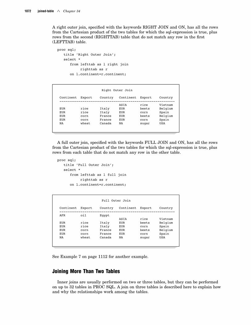
1072 joined-table 4 Chapter 34
A right outer join, specified with the keywords RIGHT JOIN and ON, has all the rowsfrom the Cartesian product of the two tables for which the sql-expression is true, plusrows from the second (RIGHTTAB) table that do not match any row in the first(LEFTTAB) table.
proc sql;title ’Right Outer Join’;select *
from lefttab as l right joinrighttab as r
on l.continent=r.continent;
Right Outer Join
Continent Export Country Continent Export Country------------------------------------------------------------
ASIA rice VietnamEUR rice Italy EUR beets BelgiumEUR rice Italy EUR corn SpainEUR corn France EUR beets BelgiumEUR corn France EUR corn SpainNA wheat Canada NA sugar USA
A full outer join, specified with the keywords FULL JOIN and ON, has all the rowsfrom the Cartesian product of the two tables for which the sql-expression is true, plusrows from each table that do not match any row in the other table.
proc sql;title ’Full Outer Join’;select *
from lefttab as l full joinrighttab as r
on l.continent=r.continent;
Full Outer Join
Continent Export Country Continent Export Country------------------------------------------------------------AFR oil Egypt
ASIA rice VietnamEUR rice Italy EUR beets BelgiumEUR rice Italy EUR corn SpainEUR corn France EUR beets BelgiumEUR corn France EUR corn SpainNA wheat Canada NA sugar USA
See Example 7 on page 1112 for another example.
Joining More Than Two Tables
Inner joins are usually performed on two or three tables, but they can be performedon up to 32 tables in PROC SQL. A join on three tables is described here to explain howand why the relationships work among the tables.

The SQL Procedure 4 joined-table 1073
In a three-way join, the sql-expression consists of two conditions: one relates the firsttable to the second table and the other relates the second table to the third table. It ispossible to break this example into stages, performing a two-way join into a temporarytable and then joining that table with the third one for the same result. However,PROC SQL can do it all in one step as shown in the next example.
The example shows the joining of three tables: COMM, PRICE, and AMOUNT. Tocalculate the total revenue from exports for each country, you need to multiply theamount exported (AMOUNT table) by the price of each unit (PRICE table), and youmust know the commodity that each country exports (COMM table).
COMM Table
Continent Export Country-----------------------------NA wheat CanadaEUR corn FranceEUR rice ItalyAFR oil Egypt
PRICE Table
Export Price------------------rice 3.56corn 3.45oil 18wheat 2.98
AMOUNT Table
Country Quantity------------------Canada 16000France 2400Italy 500Egypt 10000
proc sql;title ’Total Export Revenue’;select c.Country, p.Export, p.Price,
a.Quantity,a.quantity*p.priceas Total
from comm c, price p, amount awhere c.export=p.export
and c.country=a.country;
Total Export Revenue
Country Export Price Quantity Total------------------------------------------------Italy rice 3.56 500 1780France corn 3.45 2400 8280Egypt oil 18 10000 180000Canada wheat 2.98 16000 47680

1074 LIKE condition 4 Chapter 34
See Example 9 on page 1118 for another example.
Comparison of Joins and SubqueriesYou can often use a subquery and a join to get the same result. However, it is often
more efficient to use a join if the outer query and the subquery do not return duplicaterows. For example, the following queries produce the same result. The second query ismore efficient:
proc sql;select IDNumber, Birth
from proclib.payrollwhere IDNumber in (select idnum
from proclib.staffwhere lname like ’B%’);
proc sql;select p.IDNumber, p.Birth
from proclib.payroll p, proclib.staff swhere p.idnumber=s.idnum
and s.lname like ’B%’;
Note: PROCLIB.PAYROLL is shown in Example 2 on page 1103. 4
LIKE condition
Tests for a matching pattern.
sql-expression <NOT> LIKE sql-expression
� sql-expression is described in “sql-expression” on page 1081.
DetailsThe LIKE condition selects rows by comparing character strings with a
pattern-matching specification. It resolves to true and displays the matched string(s) ifthe left operand matches the pattern specified by the right operand.
Patterns for SearchingPatterns are composed of three classes of characters:
underscore (_)matches any single character.
percent sign (%)matches any sequence of zero or more characters.
any other charactermatches that character.
These patterns can appear before, after, or on both sides of characters that you want tomatch. The LIKE condition is case-sensitive.

The SQL Procedure 4 query-expression 1075
The following list uses these values: Smith, Smooth, Smothers, Smart, and Smuggle.
’Sm%’matches Smith, Smooth, Smothers, Smart, Smuggle.
’%th’matches Smith, Smooth.
’S__gg%’matches Smuggle.
’S_o’matches a three-letter word, so it has no matches here.
’S_o%’matches Smooth, Smothers.
’S%th’matches Smith, Smooth.
’Z’matches the single, uppercase character Z only, so it has no matches here.
Searching for Mixed-Case StringsTo search for mixed-case strings, use the UPCASE function to make all the names
uppercase before entering the LIKE condition:
upcase(name) like ’SM%’;
Note: When you are using the % character, be aware of the effect of trailing blanks.You may have to use the TRIM function to remove trailing blanks in order to matchvalues. 4
query-expression
Retrieves data from tables.
See also: “table-expression” on page 1094, “Query Expressions (Subqueries)” on page1083, and “In-Line Views” on page 1050
table-expression <set-operator table-expression>…
� table-expression is described in “table-expression” on page 1094.
� set-operator is one of the following:
INTERSECT <CORRESPONDING> <ALL>
OUTER UNION <CORRESPONDING>
UNION <CORRESPONDING> <ALL>
EXCEPT <CORRESPONDING> <ALL>

1076 query-expression 4 Chapter 34
Query Expressions and Table ExpressionsA query-expression is one or more table-expressions. Multiple table expressions are
linked by set operators. The following figure illustrates the relationship betweentable-expressions and query-expressions.
query-expression
table-expression
table-expression
set operator
SELECT clauseFROM clause(more clauses)
SELECT clauseFROM clause(more clauses)
Set OperatorsPROC SQL provides traditional set operators from relational algebra:
OUTER UNIONconcatenates the query results.
UNIONproduces all unique rows from both queries.
EXCEPTproduces rows that are part of the first query only.
INTERSECTproduces rows that are common to both query results.
A query-expression with set operators is evaluated as follows.
� Each table-expression is evaluated to produce an (internal) intermediate resulttable.
� Each intermediate result table then becomes an operand linked with a setoperator to form an expression, for example, A UNION B.
� If the query-expression involves more than two table-expressions, the result fromthe first two becomes an operand for the next set operator and operand, forexample, (A UNION B) EXCEPT C, ((A UNION B) EXCEPT C) INTERSECT D,and so on.
� Evaluating a query-expression produces a single output table.
Set operators follow this order of precedence unless they are overridden byparentheses in the expression(s): INTERSECT is evaluated first. OUTER UNION,UNION, and EXCEPT have the same level of precedence.
PROC SQL performs set operations even if the tables or views that are referred to inthe table-expressions do not have the same number of columns. The reason for this isthat the ANSI Standard for SQL requires that tables or views involved in a setoperation have the same number of columns and that the columns have matching datatypes. If a set operation is performed on a table or view that has fewer columns thanthe one(s) with which it is being linked, PROC SQL extends the table or view withfewer columns by creating columns with missing values of the appropriate data type.This temporary alteration enables the set operation to be performed correctly.

The SQL Procedure 4 query-expression 1077
CORRESPONDING (CORR) KeywordThe CORRESPONDING keyword is used only when a set operator is specified.
CORR causes PROC SQL to match the columns in table-expressions by name and notby ordinal position. Columns that do not match by name are excluded from the resulttable, except for the OUTER UNION operator. See “OUTER UNION” on page 1077.
For example, when performing a set operation on two table-expressions, PROC SQLmatches the first specified column-name (listed in the SELECT clause) from onetable-expression with the first specified column-name from the other. If CORR isomitted, PROC SQL matches the columns by ordinal position.
ALL KeywordThe set operators automatically eliminate duplicate rows from their output tables.
The optional ALL keyword preserves the duplicate rows, reduces the execution by onestep, and thereby improves the query-expression’s performance. You use it when youwant to display all the rows resulting from the table-expressions, rather than just therows that are output because duplicates have been deleted. The ALL keyword is usedonly when a set operator is also specified.
OUTER UNIONPerforming an OUTER UNION is very similar to performing the SAS DATA step
with a SET statement. The OUTER UNION concatenates the intermediate results fromthe table-expressions. Thus, the result table for the query-expression contains all therows produced by the first table-expression followed by all the rows produced by thesecond table-expression. Columns with the same name are in separate columns in theresult table.
For example, the following query expression concatenates the ME1 and ME2 tablesbut does not overlay like-named columns. Output 34.3 on page 1078 shows the result.
proc sql;title ’ME1 and ME2: OUTER UNION’;select *
from me1outer unionselect *
from me2;
ME1
IDnum Jobcode Salary Bonus--------------------------------------1400 ME1 29769 5871403 ME1 28072 3421120 ME1 28619 9861120 ME1 28619 986
ME2
IDnum Jobcode Salary----------------------------1653 ME2 351081782 ME2 353451244 ME2 36925

1078 query-expression 4 Chapter 34
Output 34.3 OUTER UNION of ME1 and ME2 Tables
ME1 and ME2: OUTER UNION
IDnum Jobcode Salary Bonus IDnum Jobcode Salary--------------------------------------------------------------------1400 ME1 29769 587 .1403 ME1 28072 342 .1120 ME1 28619 986 .1120 ME1 28619 986 .
. . 1653 ME2 35108
. . 1782 ME2 35345
. . 1244 ME2 36925
To overlay columns with the same name, use the CORRESPONDING keyword.
proc sql;title ’ME1 and ME2: OUTER UNION CORRESPONDING’;select *
from me1outer union corrselect *
from me2;
ME1 and ME2: OUTER UNION CORRESPONDING
IDnum Jobcode Salary Bonus--------------------------------------1400 ME1 29769 5871403 ME1 28072 3421120 ME1 28619 9861120 ME1 28619 9861653 ME2 35108 .1782 ME2 35345 .1244 ME2 36925 .
In the resulting concatenated table, notice the following:
� OUTER UNION CORRESPONDING retains all nonmatching columns.
� For columns with the same name, if a value is missing from the result of the firsttable-expression, the value in that column from the second table-expression isinserted.
� The ALL keyword is not used with OUTER UNION because this operator’s defaultaction is to include all rows in a result table. Thus, both rows from the table ME1where IDnum is 1120 appear in the output.
UNION
The UNION operator produces a table that contains all the unique rows that resultfrom both table-expressions. That is, the output table contains rows produced by thefirst table-expression, the second table-expression, or both.

The SQL Procedure 4 query-expression 1079
Columns are appended by position in the tables, regardless of the column names.However, the data type of the corresponding columns must match or the union will notoccur. PROC SQL issues a warning message and stops executing.
The names of the columns in the output table are the names of the columns from thefirst table-expression unless a column (such as an expression) has no name in the firsttable-expression. In such a case, the name of that column in the output table is thename of the respective column in the second table-expression.
In the following example, PROC SQL combines the two tables:
proc sql;title ’ME1 and ME2: UNION’;select *
from me1unionselect *
from me2;
ME1 and ME2: UNION
IDnum Jobcode Salary Bonus--------------------------------------1120 ME1 28619 9861244 ME2 36925 .1400 ME1 29769 5871403 ME1 28072 3421653 ME2 35108 .1782 ME2 35345 .
In the following example, ALL includes the duplicate row from ME1. In addition, ALLchanges the sorting by specifying that PROC SQL make one pass only. Thus, the valuesfrom ME2 are simply appended to the values from ME1.
proc sql;title ’ME1 and ME2: UNION ALL’;select *
from me1union allselect *
from me2;
ME1 and ME2: UNION ALL
IDnum Jobcode Salary Bonus--------------------------------------1400 ME1 29769 5871403 ME1 28072 3421120 ME1 28619 9861120 ME1 28619 9861653 ME2 35108 .1782 ME2 35345 .1244 ME2 36925 .
See Example 5 on page 1108 for another example.

1080 query-expression 4 Chapter 34
EXCEPT
The EXCEPT operator produces (from the first table-expression) an output table thathas unique rows that are not in the second table-expression. If the intermediate resultfrom the first table-expression has at least one occurrence of a row that is not in theintermediate result of the second table-expression, that row (from the firsttable-expression) is included in the result table.
In the following example, the IN_USA table contains flights to cities within andoutside the USA. The OUT_USA table contains flights only to cities outside the USA.This example returns only the rows from IN_USA that are not also in OUT_USA:
proc sql;title ’Flights from IN_USA’;select * from in_usaexceptselect * from out_usa;
IN_USA
Flight Dest------------------145 ORD156 WAS188 LAX193 FRA207 LON
OUT_USA
Flight Dest------------------193 FRA207 LON311 SJA
Flights from IN_USA
Flight Dest------------------145 ORD156 WAS188 LAX
INTERSECT
The INTERSECT operator produces an output table that has rows that are commonto both tables. For example, using the IN_USA and OUT_USA tables shown above, thefollowing example returns rows that are in both tables:
proc sql;title ’Flights from IN_USA and OUT_USA’;select * from in_usaintersectselect * from out_usa;

The SQL Procedure 4 sql-expression 1081
Flights from IN_USA and OUT_USA
Flight Dest------------------193 FRA207 LON
sql-expression
Produces a value from a sequence of operands and operators.
operand operator operand
� operand is one of the following:
� constant is a number or a quoted character string (or other special notation)that indicates a fixed value. Constants are also called literals. Constants aredescribed in SAS Language Reference: Dictionary.
� column-name is described in “column-name” on page 1061.
� SAS-function is almost any SAS function. Functions are described in SASLanguage Reference: Dictionary.
� The ANSI SQL function COALESCE is supported.
� summary-function is described in “summary-function” on page 1088.
� query-expression is described in “query-expression” on page 1075.
� USER is a literal that references the userid of the person who submitted theprogram. The userid that is returned is operating environment-dependent,but PROC SQL uses the same value that the &SYSJOBID macro variablehas on the operating environment.
� operator is described in “Operators and the Order of Evaluation” on page 1082.
Note: SAS functions, including summary functions, can stand alone as SQLexpressions. For example
select min(x) from table;
select scan(y,4) from table;
4
SAS FunctionsPROC SQL supports the same SAS functions as the DATA step, except for the
functions LAG, DIF, and SOUND. For example, the SCAN function is used in thefollowing query:
select style, scan(street,1) format=$15.from houses;
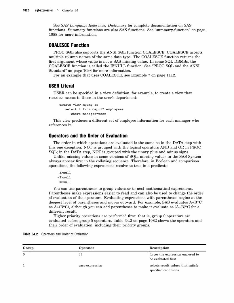
1082 sql-expression 4 Chapter 34
See SAS Language Reference: Dictionary for complete documentation on SASfunctions. Summary functions are also SAS functions. See “summary-function” on page1088 for more information.
COALESCE FunctionPROC SQL also supports the ANSI SQL function COALESCE. COALESCE accepts
multiple column names of the same data type. The COALESCE function returns thefirst argument whose value is not a SAS missing value. In some SQL DBMSs, theCOALESCE function is called the IFNULL function. See “PROC SQL and the ANSIStandard” on page 1098 for more information.
For an example that uses COALESCE, see Example 7 on page 1112.
USER LiteralUSER can be specified in a view definition, for example, to create a view that
restricts access to those in the user’s department:
create view myemp asselect * from dept12.employees
where manager=user;
This view produces a different set of employee information for each manager whoreferences it.
Operators and the Order of EvaluationThe order in which operations are evaluated is the same as in the DATA step with
this one exception: NOT is grouped with the logical operators AND and OR in PROCSQL; in the DATA step, NOT is grouped with the unary plus and minus signs.
Unlike missing values in some versions of SQL, missing values in the SAS Systemalways appear first in the collating sequence. Therefore, in Boolean and comparisonoperations, the following expressions resolve to true in a predicate:
3>null-3>null
0>null
You can use parentheses to group values or to nest mathematical expressions.Parentheses make expressions easier to read and can also be used to change the orderof evaluation of the operators. Evaluating expressions with parentheses begins at thedeepest level of parentheses and moves outward. For example, SAS evaluates A+B*Cas A+(B*C), although you can add parentheses to make it evaluate as (A+B)*C for adifferent result.
Higher priority operations are performed first: that is, group 0 operators areevaluated before group 5 operators. Table 34.2 on page 1082 shows the operators andtheir order of evaluation, including their priority groups.
Table 34.2 Operators and Order of Evaluation
Group Operator Description
0 ( ) forces the expression enclosed tobe evaluated first
1 case-expression selects result values that satisfyspecified conditions

The SQL Procedure 4 sql-expression 1083
Group Operator Description
2 ** raises to a power
unary +, unary - indicates a positive or negativenumber
3 * multiplies
/ divides
4 + adds
− subtracts
5 || concatenates
6 <NOT> BETWEEN condition See “BETWEEN condition” onpage 1057.
<NOT> CONTAINS condition see “CONTAINS condition” onpage 1062.
<NOT> EXISTS condition See “EXISTS condition” on page1066.
<NOT> IN condition See “IN condition” on page 1067.
IS <NOT> condition See “IS condition” on page 1067.
<NOT> LIKE condition See “LIKE condition” on page1074.
7 =, eq equals
=, ^=, < >, ne does not equal
>, gt is greater than
<, lt is less than
>=, ge is greater than or equal to
<=, le is less than or equal to
=* sounds like (use with characteroperands only). See Example 11on page 1122.
8 &, AND indicates logical AND
9 |, OR indicates logical OR
10 , ^, NOT indicates logical NOT
Symbols for operators may vary, depending on the operating environment. See SASLanguage Reference: Dictionary for more information on operators and expressions.
Query Expressions (Subqueries)
Query-expressions are called subqueries when used in WHERE or HAVING clauses.A subquery is a query-expression that is nested as part of another query-expression. Asubquery selects one or more rows from a table based on values in another table.
Depending on the clause that contains it, a subquery can return a single value ormultiple values. If more than one subquery is used in a query-expression, the innermostquery is evaluated first, then the next innermost query, and so on, moving outward.

1084 sql-expression 4 Chapter 34
PROC SQL allows a subquery (contained in parentheses) at any point in anexpression where a simple column value or constant can be used. In this case, asubquery must return a single value, that is, one row with only one column. When asubquery returns one value, you can name the value with a column alias and refer to itby that name elsewhere in the query. This is useful for replacing values with othervalues returned using a subquery.
The following is an example of a subquery that returns one value. This PROC SQLstep subsets the PROCLIB.PAYROLL table based on information in thePROCLIB.STAFF table. (PROCLIB.PAYROLL is shown in Example 2 on page 1103, andPROCLIB.STAFF is shown in Example 4 on page 1106.) PROCLIB.PAYROLL containsemployee identification numbers (IdNumber) and their salaries (Salary) but does notcontain their names. If you want to return only the row from PROCLIB.PAYROLL forone employee, you can use a subquery that queries the PROCLIB.STAFF table, whichcontains the employees’ identification numbers and their names (Lname and Fname).
options ls=64 nodate nonumber;proc sql;
title ’Information for Earl Bowden’;select *
from proclib.payrollwhere idnumber=
(select idnumfrom proclib.staffwhere upcase(lname)=’BOWDEN’);
Information for Earl Bowden
IdNumber Sex Jobcode Salary Birth Hired------------------------------------------------1403 M ME1 28072 28JAN69 21DEC91
Subqueries can return multiple values. The following example uses the tablesPROCLIB.DELAY and PROCLIB.MARCH. These tables contain information about thesame flights and have the Flight column in common. The following subquery returns allthe values for Flight in PROCLIB.DELAY for international flights. The values from thesubquery complete the WHERE clause in the outer query. Thus, when the outer queryis executed, only the international flights from PROCLIB.MARCH are in the output.
options ls=64 nodate nonumber;proc sql outobs=5;
title ’International Flights from’;title2 ’PROCLIB.MARCH’;select Flight, Date, Dest, Boarded
from proclib.marchwhere flight in
(select flightfrom proclib.delaywhere destype=’International’);

The SQL Procedure 4 sql-expression 1085
International Flights fromPROCLIB.MARCH
Flight Date Dest Boarded-------------------------------219 01MAR94 LON 198622 01MAR94 FRA 207132 01MAR94 YYZ 115271 01MAR94 PAR 138219 02MAR94 LON 147
Sometimes it is helpful to compare a value with a set of values returned by a subquery.The keywords ANY or ALL can be specified before a subquery when the subquery is theright-hand operand of a comparison. If ALL is specified, the comparison is true only ifit is true for all values returned by the subquery. If a subquery returns no rows, theresult of an ALL comparison is true for each row of the outer query.
If ANY is specified, the comparison is true if it is true for any one of the valuesreturned by the subquery. If a subquery returns no rows, the result of an ANYcomparison is false for each row of the outer query.
The following example selects all those in PROCLIB.PAYROLL who earn more thanthe highest paid ME3:
options ls=64 nodate nonumber ;proc sql;title ‘‘Employees who Earn More than’’;title2 ‘‘All ME’s’’;
select *from proclib.payrollwhere salary > all (select salary
from proclib.payrollwhere jobcode=’ME3’);
Employees who Earn More thanAll ME’s
IdNumber Sex Jobcode Salary Birth Hired------------------------------------------------1333 M PT2 88606 30MAR61 10FEB811739 M PT1 66517 25DEC64 27JAN911428 F PT1 68767 04APR60 16NOV911404 M PT2 91376 24FEB53 01JAN801935 F NA2 51081 28MAR54 16OCT811905 M PT1 65111 16APR72 29MAY921407 M PT1 68096 23MAR69 18MAR901410 M PT2 84685 03MAY67 07NOV861439 F PT1 70736 06MAR64 10SEP901545 M PT1 66130 12AUG59 29MAY901106 M PT2 89632 06NOV57 16AUG841442 F PT2 84536 05SEP66 12APR881417 M NA2 52270 27JUN64 07MAR891478 M PT2 84203 09AUG59 24OCT901556 M PT1 71349 22JUN64 11DEC91

1086 sql-expression 4 Chapter 34
Employees who Earn More thanAll ME’s
IdNumber Sex Jobcode Salary Birth Hired------------------------------------------------1352 M NA2 53798 02DEC60 16OCT861890 M PT2 91908 20JUL51 25NOV791107 M PT2 89977 09JUN54 10FEB791830 F PT2 84471 27MAY57 29JAN831928 M PT2 89858 16SEP54 13JUL901076 M PT1 66558 14OCT55 03OCT91
Note: See the first item in “Subqueries and Efficiency” on page 1087 for a noteabout efficiency when using ALL. 4
Correlated SubqueriesIn a correlated subquery, the WHERE expression in a subquery refers to values in a
table in the outer query. The correlated subquery is evaluated for each row in the outerquery. With correlated subqueries, PROC SQL executes the subquery and the outerquery together.
The following example uses the PROCLIB.DELAY and PROCLIB.MARCH tables. ADATA step“PROCLIB.DELAY” on page 1506 creates PROCLIB.DELAY.PROCLIB.MARCH is shown in Example 13 on page 1126. PROCLIB.DELAY has theFlight, Date, Orig, and Dest columns in common with PROCLIB.MARCH:
proc sql outobs=5;title ’International Flights’;select *
from proclib.marchwhere ’International’ in
(select destypefrom proclib.delaywhere march.Flight=delay.Flight);
The subquery resolves by substituting every value for MARCH.Flight into thesubquery’s WHERE clause, one row at a time. For example, when MARCH.Flight= 219,the subquery resolves as follows:
1 PROC SQL retrieves all the rows from DELAY where Flight= 219 and passes theirDESTYPE values to the WHERE clause.
2 PROC SQL uses the DESTYPE values to complete the WHERE clause:
where ’International’ in(’International’,’International’, ...)
3 The WHERE clause checks to see if International is in the list. Because it is, allrows from MARCH that have a value of 219 for Flight become part of the output.
Output 34.4 on page 1086 contains the rows from MARCH for international flightsonly.

The SQL Procedure 4 sql-expression 1087
Output 34.4 International Flights for March
International Flights
Flight Date Depart Orig Dest Miles Boarded Capacity-----------------------------------------------------------------219 01MAR94 9:31 LGA LON 3442 198 250622 01MAR94 12:19 LGA FRA 3857 207 250132 01MAR94 15:35 LGA YYZ 366 115 178271 01MAR94 13:17 LGA PAR 3635 138 250219 02MAR94 9:31 LGA LON 3442 147 250
Subqueries and Efficiency
� Use the MAX function in a subquery instead of the ALL keyword before thesubquery. For example, the following queries produce the same result, but thesecond query is more efficient:
proc sql;select * from proclib.payrollwhere salary> all(select salary
from proclib.payrollwhere jobcode=’ME3’);
proc sql;select * from proclib.payrollwhere salary> (select max(salary)
from proclib.payrollwhere jobcode=’ME3’);
� With subqueries, use IN instead of EXISTS when possible. For example, thefollowing queries produce the same result, but the second query is more efficient:
proc sql;select *
from proclib.payroll pwhere exists (select *
from staff swhere p.idnum=s.idnum
and state=’CT’);
proc sql;select *
from proclib.payrollwhere idnum in (select idnum
from staffwhere state=’CT’);

1088 summary-function 4 Chapter 34
summary-function
Performs statistical summary calculations.
Restriction: A summary function cannot appear in an ON clause or a WHERE clause.See also: GROUP BY on page 1052, HAVING Clause on page 1053, SELECT Clause onpage 1045, and “table-expression” on page 1094Featured in: Example 8 on page 1116, Example 12 on page 1124, and Example 15 onpage 1131
summary-function (<DISTINCT|ALL> sql-expression)
� sql-expression is described in “sql-expression” on page 1081.
Summarizing DataSummary functions produce a statistical summary of the entire table or view listed
in the FROM clause or for each group specified in a GROUP BY clause. If GROUP BYis omitted, all the rows in the table or view are considered to be a single group. Thesefunctions reduce all the values in each row or column in a table to one summarizing oraggregate value. For this reason, these functions are often called aggregate functions.For example, the sum (one value) of a column results from the addition of all the valuesin the column.
Function Names and the Corresponding StatisticsSome functions have more than one name to accommodate both SAS and SQL
conventions:
AVG, MEANmeans or average of values
COUNT, FREQ, Nnumber of nonmissing values
CSScorrected sum of squares
CVcoefficient of variation (percent)
MAXlargest value
MINsmallest value
NMISSnumber of missing values
PRTprobability of a greater absolute value of Student’s t
RANGErange of values

The SQL Procedure 4 summary-function 1089
STDstandard deviation
STDERRstandard error of the mean
SUMsum of values
SUMWGTsum of the WEIGHT variable values*
TStudent’s t value for testing the hypothesis that the population mean is zero
USSuncorrected sum of squares
VARvariance
For a description and the formulas used for these statistics, see Appendix 1, “SASElementary Statistics Procedures,” on page 1457
Counting RowsThe COUNT function counts rows. COUNT(*) returns the total number of rows in a
group or in a table. If you use a column name as an argument to COUNT, the result isthe total number of rows in a group or in a table that have a nonmissing value for thatcolumn. If you want to count the unique values in a column, specifyCOUNT(DISTINCT column).
If the SELECT clause of a table-expression contains one or more summary functionsand that table-expression resolves to no rows, then the summary function results aremissing values. The following are exceptions that return zeros:
COUNT(*)COUNT(<DISTINCT> sql-expression)NMISS(<DISTINCT> sql-expression)
See Example 8 on page 1116 and Example 15 on page 1131 for examples.
Calculating Statistics Based on the Number of ArgumentsThe number of arguments specified in a summary function affects how the
calculation is performed. If you specify a single argument, the values in the column arecalculated. If you specify multiple arguments, the arguments or columns listed arecalculated for each row. For example, consider calculations on the following table.
proc sql;title ’Summary Table’;select * from summary;
* Currently, there is no way to designate a WEIGHT variable for a table in PROC SQL. Thus, each row (or observation) has aweight of 1.

1090 summary-function 4 Chapter 34
Summary Table
X Y Z----------------------------
1 3 42 4 58 9 44 5 4
If you use one argument in the function, the calculation is performed on that columnonly. If you use more than one argument, the calculation is performed on each row ofthe specified columns. In the following PROC SQL step, the MIN and MAX functionsreturn the minimum and maximum of the columns they are used with. The SUMfunction returns the sum of each row of the columns specified as arguments:
proc sql;select min(x) as Colmin_x,
min(y) as Colmin_y,max(z) as Colmax_z,sum(x,y,z) as Rowsum
from summary;
Summary Table
Colmin_x Colmin_y Colmax_z Rowsum--------------------------------------
1 3 5 81 3 5 111 3 5 211 3 5 13
Remerging DataWhen you use a summary function in a SELECT clause or a HAVING clause, you
may see the following message in the SAS log:
NOTE: The query requires remerging summarystatistics back with the originaldata.
The process of remerging involves two passes through the data. On the first pass,PROC SQL
� calculates and returns the value of summary functions. It then uses the result tocalculate the arithmetic expressions in which the summary function participates.
� groups data according to the GROUP BY clause.
On the second pass, PROC SQL retrieves any additional columns and rows that itneeds to show in the output.
The following examples use the PROCLIB.PAYROLL table (shown in Example 2 onpage 1103) to show when remerging of data is and is not necessary.
The first query requires remerging. The first pass through the data groups the databy Jobcode and resolves the AVG function for each group. However, PROC SQL mustmake a second pass in order to retrieve the values of IdNumber and Salary.

The SQL Procedure 4 summary-function 1091
proc sql outobs=10;title ’Salary Information’;title2 ’(First 10 Rows Only)’;select IdNumber, Jobcode, Salary,
avg(salary) as AvgSalaryfrom proclib.payrollgroup by jobcode;
Salary Information(First 10 Rows Only)
IdNumber Jobcode Salary AvgSalary------------------------------------1845 BCK 25996 25794.221673 BCK 25477 25794.221834 BCK 26896 25794.221389 BCK 25028 25794.221100 BCK 25004 25794.221677 BCK 26007 25794.221663 BCK 26452 25794.221383 BCK 25823 25794.221704 BCK 25465 25794.221132 FA1 22413 23039.36
You can change the previous query to return only the average salary for each jobcode.The following query does not require remerging because the first pass of the data doesthe summarizing and the grouping. A second pass is not necessary.
proc sql outobs=10;title ’Average Salary for Each Jobcode’;select Jobcode, avg(salary) as AvgSalaryfrom proclib.payrollgroup by jobcode;
Average Salary for Each Jobcode
Jobcode AvgSalary------------------BCK 25794.22FA1 23039.36FA2 27986.88FA3 32933.86ME1 28500.25ME2 35576.86ME3 42410.71NA1 42032.2NA2 52383PT1 67908
When you use the HAVING clause, PROC SQL may have to remerge data to resolve theHAVING expression.
First, consider a query that uses HAVING but that does not require remerging. Thequery groups the data by values of Jobcode, and the result contains one row for eachvalue of Jobcode and summary information for people in each Jobcode. On the first

1092 summary-function 4 Chapter 34
pass, the summary functions provide values for the Number, Average Age, and AverageSalary columns. The first pass provides everything that PROC SQL needs to resolvethe HAVING clause, so no remerging is necessary.
proc sql outobs=10;title ’Summary Information for Each Jobcode’;title2 ’(First 10 Rows Only)’;
select Jobcode,count(jobcode) as number
label=’Number’,avg(int((today()-birth)/365.25))
as avgage format=2.label=’Average Age’,
avg(salary) as avgsal format=dollar8.label=’Average Salary’
from proclib.payrollgroup by jobcodehaving avgage ge 30;
Summary Information for Each Jobcode 1(First 10 Rows Only)
Average AverageJobcode Number Age Salary------------------------------------BCK 9 33 $25,794FA1 11 30 $23,039FA2 16 34 $27,987FA3 7 36 $32,934ME1 8 31 $28,500ME2 14 37 $35,577ME3 7 39 $42,411NA2 3 39 $52,383PT1 8 35 $67,908PT2 10 40 $87,925
In the following query, PROC SQL remerges the data because the HAVING clause usesthe SALARY column in the comparison and SALARY is not in the GROUP BY clause.
proc sql outobs=10;title ’Employees who Earn More than the’;title2 ’Average for Their Jobcode’;title3 ’(First 10 Rows Only)’;
select Jobcode, Salary,avg(salary) as AvgSalary
from proclib.payrollgroup by jobcodehaving salary > AvgSalary;
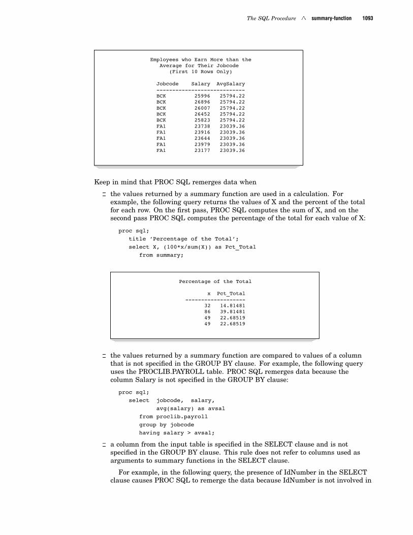
The SQL Procedure 4 summary-function 1093
Employees who Earn More than theAverage for Their Jobcode
(First 10 Rows Only)
Jobcode Salary AvgSalary----------------------------BCK 25996 25794.22BCK 26896 25794.22BCK 26007 25794.22BCK 26452 25794.22BCK 25823 25794.22FA1 23738 23039.36FA1 23916 23039.36FA1 23644 23039.36FA1 23979 23039.36FA1 23177 23039.36
Keep in mind that PROC SQL remerges data when
� the values returned by a summary function are used in a calculation. Forexample, the following query returns the values of X and the percent of the totalfor each row. On the first pass, PROC SQL computes the sum of X, and on thesecond pass PROC SQL computes the percentage of the total for each value of X:
proc sql;title ’Percentage of the Total’;select X, (100*x/sum(X)) as Pct_Total
from summary;
Percentage of the Total
x Pct_Total-------------------
32 14.8148186 39.8148149 22.6851949 22.68519
� the values returned by a summary function are compared to values of a columnthat is not specified in the GROUP BY clause. For example, the following queryuses the PROCLIB.PAYROLL table. PROC SQL remerges data because thecolumn Salary is not specified in the GROUP BY clause:
proc sql;select jobcode, salary,
avg(salary) as avsalfrom proclib.payrollgroup by jobcodehaving salary > avsal;
� a column from the input table is specified in the SELECT clause and is notspecified in the GROUP BY clause. This rule does not refer to columns used asarguments to summary functions in the SELECT clause.
For example, in the following query, the presence of IdNumber in the SELECTclause causes PROC SQL to remerge the data because IdNumber is not involved in

1094 table-expression 4 Chapter 34
grouping or summarizing during the first pass. In order for PROC SQL to retrievethe values for IdNumber, it must make a second pass through the data.
proc sql;select IdNumber, jobcode,
avg(salary) as avsalfrom proclib.payrollgroup by jobcode;
table-expression
Defines part or all of a query-expression.
See also: “query-expression” on page 1075
SELECT <DISTINCT> object-item<,object-item>…
<INTO :macro-variable-specification<, :macro-variable-specification>…>
FROM from-list
<WHERE sql-expression>
<GROUP BY group-by-item <,group-by-item>…>
<HAVING sql-expression>
See “SELECT Statement” on page 1044 for complete information on the SELECTstatement.
DetailsA table-expression is a SELECT statement. It is the fundamental building block of
most SQL procedure statements. You can combine the results of multipletable-expressions with set operators, which creates a query-expression. Use oneORDER BY clause for an entire query-expression. Place a semicolon only at the end ofthe entire query-expression. A query-expression is often only one SELECT statement ortable-expression.
Concepts
Using SAS Data Set Options with PROC SQLPROC SQL can apply most of the SAS data set options, such as KEEP= and DROP=,
to tables or SAS/ACCESS views. In the SQL procedure, SAS data set options that areseparated by spaces are enclosed in parentheses, and they follow immediately after thetable or SAS/ACCESS view name. You can also use SAS data set options on tables orSAS/ACCESS views listed in the FROM clause of a query. In the following PROC SQL

The SQL Procedure 4 Connecting to a DBMS using the LIBNAME Statement 1095
step, RENAME= renames LNAME to LASTNAME for the STAFF1 table. OBS=restricts the number of rows written to STAFF1 to 15:
proc sql;create table
staff1(rename=(lname=lastname)) asselect *
from staff(obs=15);
You cannot use SAS data set options with DICTIONARY tables becauseDICTIONARY tables are read-only objects.
The only SAS data set options that you can use with PROC SQL views are those thatassign and provide SAS passwords: READ=, WRITE=, ALTER=, and PW=.
See SAS Language Reference: Dictionary for a description of SAS data set options.
Connecting to a DBMS Using the SQL Procedure Pass-Through FacilityThe SQL Procedure Pass-Through Facility enables you to send DBMS-specific SQL
statements directly to a DBMS for execution. The Pass-Through Facility uses a SAS/ACCESS interface engine to connect to the DBMS. Therefore, you must have SAS/ACCESS software installed for your DBMS.
You submit SQL statements that are DBMS-specific. For example, you passTransact-SQL statements to a SYBASE database. The Pass-Through Facility’s basicsyntax is the same for all the DBMSs. Only the statements that are used to connect tothe DBMS and the SQL statements are DBMS-specific.
With the Pass-Through Facility, you can perform the following tasks:� establish a connection with the DBMS using a CONNECT statement and
terminate the connection with the DISCONNECT statement.� send nonquery DBMS-specific SQL statements to the DBMS using the EXECUTE
statement.� retrieve data from the DBMS to be used in a PROC SQL query with the
CONNECTION TO component in a SELECT statement’s FROM clause.
You can use the Pass-Through Facility statements in a query, or you can store themin a PROC SQL view. When a view is stored, any options that are specified in thecorresponding CONNECT statement are also stored. Thus, when the PROC SQL viewis used in a SAS program, the SAS System can automatically establish the appropriateconnection to the DBMS.
See “CONNECT Statement” on page 1033, “DISCONNECT Statement” on page 1040,“EXECUTE Statement” on page 1042, “CONNECTION TO” on page 1062, and yourSAS/ACCESS documentation.
Return CodesAs you use PROC SQL statements that are available in the Pass-Through Facility,
any errors are written to the SAS log. The return codes and messages that aregenerated by the Pass-Through Facility are available to you through the SQLXRC andSQLXMSG macro variables. Both macro variables are described in “Using MacroVariables Set by PROC SQL” on page 1096.
Connecting to a DBMS using the LIBNAME StatementFor many DBMSs, you can directly access DBMS data by assigning a libref to the
DBMS using the SAS/ACCESS LIBNAME statement. Once you have associated a libref

1096 Using Macro Variables Set by PROC SQL 4 Chapter 34
with the DBMS, you can specify a DBMS table in a two-level SAS name and work withthe table like any SAS data set. You can also embed the LIBNAME statement in aPROC SQL view (see “CREATE VIEW Statement” on page 1037).
PROC SQL will take advantage of the capabilities of a DBMS by passing it certainoperations whenever possible. For example, before implementing a join, PROC SQLchecks to see if the DBMS can do the join. If it can, PROC SQL passes the join to theDBMS. This increases performance by reducing data movement and translation. If theDBMS cannot do the join, PROC SQL processes the join. Using the SAS/ACCESSLIBNAME statement can often provide you with the performance benefits of the SQLProcedure Pass-Through Facility without having to write DBMS-specific code.
To use the SAS/ACCESS LIBNAME statement, you must have SAS/ACCESSinstalled for your DBMS. For more information on the SAS/ACCESS LIBNAMEstatement, refer to your SAS/ACCESS documentation.
Using Macro Variables Set by PROC SQLPROC SQL sets up macro variables with certain values after it executes each
statement. These macro variables can be tested inside a macro to determine whether tocontinue executing the PROC SQL step. SAS/AF software users can also test them in aprogram after an SQL SUBMIT block of code, using the SYMGET function.
After each PROC SQL statement has executed, the following macro variables areupdated with these values:
SQLOBScontains the number of rows executed by an SQL procedure statement. Forexample, it contains the number of rows formatted and displayed in SAS output bya SELECT statement or the number of rows deleted by a DELETE statement.
SQLRCcontains the following status values that indicate the success of the SQL procedurestatement:
0PROC SQL statement completed successfully with no errors.
4PROC SQL statement encountered a situation for which it issued a warning.The statement continued to execute.
8PROC SQL statement encountered an error. The statement stoppedexecution at this point.
12PROC SQL statement encountered an internal error, indicating a bug inPROC SQL that should be reported to SAS Institute. These errors can occuronly during compile time.
16PROC SQL statement encountered a user error. This error code is used, forexample, when a subquery (that can only return a single value) evaluates tomore than one row. These errors can only be detected during run time.
24PROC SQL statement encountered a system error. This error is used, forexample, if the system cannot write to a PROC SQL table because the disk isfull. These errors can occur only during run time.

The SQL Procedure 4 Updating PROC SQL and SAS/ACCESS Views 1097
28PROC SQL statement encountered an internal error, indicating a bug inPROC SQL that should be reported to SAS Institute. These errors can occuronly during run time.
SQLOOPScontains the number of iterations that the inner loop of PROC SQL executes. Thenumber of iterations increases proportionally with the complexity of the query. Seealso the description of the LOOPS option on page 1029.
SQLXRCcontains the DBMS-specific return code that is returned by the Pass-ThroughFacility.
SQLXMSGcontains descriptive information and the DBMS-specific return code for the errorthat is returned by the Pass-Through Facility.
This example retrieves the data but does not display them in SAS output because ofthe NOPRINT option in the PROC SQL statement. The %PUT macro statementdisplays the macro variables values.
proc sql noprint;select *
from proclib.payroll;
%put sqlobs=**&sqlobs**sqloops=**&sqloops**sqlrc=**&sqlrc**;
The message in Output 34.5 on page 1097 appears in the SAS log and gives you themacros’ values.
Output 34.5 PROC SQL Macro Variable Values
1 options ls=80;2 proc sql noprint;3 select *4 from proclib.payroll;56 %put sqlobs=**&sqlobs**7 sqloops=**&sqloops**8 sqlrc=**&sqlrc**;sqlobs=**1** sqloops=**11** sqlrc=**0**
Updating PROC SQL and SAS/ACCESS Views
You can update PROC SQL and SAS/ACCESS views using the INSERT, DELETE,and UPDATE statements, under the following conditions.
� If the view accesses a DBMS table, you must have been granted the appropriateauthorization by the external database management system (for example, DB2).You must have installed the SAS/ACCESS software for your DBMS. See the SAS/ACCESS interface guide for your DBMS for more information on SAS/ACCESSviews.

1098 PROC SQL and the ANSI Standard 4 Chapter 34
� You can update only a single table through a view. The table cannot be joined toanother table or linked to another table with a set-operator. The view cannotcontain a subquery.
� You can update a column in a view using the column’s alias, but you cannotupdate a derived column, that is, a column produced by an expression. In thefollowing example, you can update the column SS, but not WeeklySalary.
create view EmployeeSalaries asselect Employee, SSNumber as SS,
Salary/52 as WeeklySalaryfrom employees;
� You cannot update a view containing an ORDER BY.
PROC SQL and the ANSI StandardPROC SQL follows most of the guidelines set by the American National Standards
Institute (ANSI) in its implementation of SQL. However, it is not fully compliant withthe current ANSI Standard for SQL.*
The SQL research project at SAS Institute has focused primarily on the expressivepower of SQL as a query language. Consequently, some of the database features of SQLhave not yet been implemented in the SAS System.
This section describes� enhancements to SQL that SAS Institute has made through PROC SQL� the ways in which PROC SQL differs from the current ANSI Standard for SQL.
SQL Procedure EnhancementsMost of the enhancements described here are required by the current ANSI Standard.
Reserved WordsPROC SQL reserves very few keywords and then only in certain contexts. The ANSI
Standard reserves all SQL keywords in all contexts. For example, according to theStandard you cannot name a column GROUP because of the keywords GROUP BY.
The following words are reserved in PROC SQL:� The keyword CASE is always reserved; its use in the CASE expression (an SQL2
feature) precludes its use as a column name.If you have a column named CASE in a table and you want to specify it in a
PROC SQL step, you can use the SAS data set option RENAME= to rename thatcolumn for the duration of the query. You can also surround CASE in doublequotes (“CASE”) and set the PROC SQL option DQUOTE=ANSI.
� The keywords AS, ON, FULL, JOIN, LEFT, FROM, WHEN, WHERE, ORDER,GROUP, RIGHT, INNER, OUTER, UNION, EXCEPT, HAVING, and INTERSECTcannot normally be used for table aliases. These keywords all introduce clausesthat appear after a table name. Since the alias is optional, PROC SQL deals withthis ambiguity by assuming that any one of these words introduces thecorresponding clause and is not the alias. If you want to use one of these keywordsas an alias, use the PROC SQL option DQUOTE=ANSI.
* International Organization for Standardization (ISO): Database SQL. Document ISO/IEC 9075:1992. Also available asAmerican National Standards Institute (ANSI) Document ANSI X3.135-1992.

The SQL Procedure 4 SQL Procedure Enhancements 1099
� The keyword USER is reserved for the current userid. If you have a columnnamed USER in a table and you want to specify it in a PROC SQL step, you canuse the SAS data set option RENAME= to rename that column for the duration ofthe query. You can also surround USER in double quotes (“USER”) and set thePROC SQL option DQUOTE=ANSI.
Column ModifiersPROC SQL supports the SAS System’s INFORMAT=, FORMAT=, and LABEL=
modifiers for expressions within the SELECT clause. These modifiers control the formatin which output data are displayed and labeled.
Alternate Collating SequencesPROC SQL allows you to specify an alternate collating (sorting) sequence to be used
when you specify the ORDER BY clause. See the description of the SORTSEQ= optionin “PROC SQL Statement” on page 1027 for more information.
ORDER BY Clause in a View DefinitionPROC SQL permits you to specify an ORDER BY clause in a CREATE VIEW
statement. When the view is queried, its data are always sorted according to thespecified order unless a query against that view includes a different ORDER BY clause.See “CREATE VIEW Statement” on page 1037 for more information.
In-Line ViewsThe ability to code nested query-expressions in the FROM clause is a requirement of
the ANSI Standard. PROC SQL supports such nested coding.
Outer JoinsThe ability to include columns that both match and do not match in a join-expression
is a requirement of the ANSI Standard. PROC SQL supports this ability.
Arithmetic OperatorsPROC SQL supports the SAS System exponentiation (**) operator. PROC SQL uses
the notation < > to mean not equal.
Orthogonal ExpressionsPROC SQL permits the combination of comparison, Boolean, and algebraic
expressions. For example, (X=3)*7 yields a value of 7 if X=3 is true because true isdefined to be 1. If X=3 is false, it resolves to 0 and the entire expression yields a valueof 0.
PROC SQL permits a subquery in any expression. This feature is required by theANSI Standard. Therefore, you can have a subquery on the left side of a comparisonoperator in the WHERE expression.
PROC SQL permits you to order and group data by any kind of mathematicalexpression (except those including summary functions) using ORDER BY and GROUPBY clauses. You can also group by an expression that appears on the SELECT clauseby using the integer that represents the expression’s ordinal position in the SELECTclause. You are not required to select the expression by which you are grouping or

1100 SQL Procedure Omissions 4 Chapter 34
ordering. See ORDER BY Clause on page 1053 and GROUP BY Clause on page 1052for more information.
Set OperatorsThe set operators UNION, INTERSECT, and EXCEPT are required by the ANSI
Standard. PROC SQL provides these operators plus the OUTER UNION operator.The ANSI Standard also requires that the tables being operated upon all have the
same number of columns with matching data types. The SQL procedure works ontables that have the same number of columns, as well as on those that do not, bycreating virtual columns so that a query can evaluate correctly. See “query-expression”on page 1075 for more information.
Statistical FunctionsPROC SQL supports many more summary functions than required by the ANSI
Standard for SQL.PROC SQL supports the remerging of summary function results into the table’s
original data. For example, computing the percentage of total is achieved with 100*x/SUM(x) in PROC SQL. See “summary-function” on page 1088 for more information onthe available summary functions and remerging data.
SAS System FunctionsPROC SQL supports all the functions available to the SAS DATA step, except for
LAG, DIF, and SOUND. Other SQL databases support their own set of functions.
SQL Procedure OmissionsPROC SQL differs from the ANSI Standard for SQL in the following ways.
COMMIT StatementThe COMMIT statement is not supported.
ROLLBACK StatementThe ROLLBACK statement is not supported. The UNDO_POLICY= option in the
PROC SQL statement addresses rollback. See the description of the UNDO_POLICY=option in “PROC SQL Statement” on page 1027 for more information.
Identifiers and Naming ConventionsIn the SAS System, table names, column names, and aliases are limited to 32
characters and can contain mixed case. For more information on SAS namingconventions, see SAS Language Reference: Dictionary. The ANSI Standard for SQLallows longer names.
Granting User PrivilegesThe GRANT statement, PRIVILEGES keyword, and authorization-identifier features
of SQL are not supported. You may want to use operating environment-specific meansof security instead.

The SQL Procedure 4 Program 1101
Three-Valued LogicANSI-compatible SQL has three-valued logic, that is, special cases for handling
comparisons involving NULL values. Any value compared with a NULL valueevaluates to NULL.
PROC SQL follows the SAS System convention for handling missing values: whennumeric NULL values are compared to non-NULL numbers, the NULL values are lessthan or smaller than all the non-NULL values; when character NULL values arecompared to non-NULL characters, the character NULL values are treated as a stringof blanks.
Embedded SQLCurrently there is no provision for embedding PROC SQL statements in other SAS
programming environments, such as the DATA step or SAS/IML software.
Examples
Example 1: Creating a Table and Inserting Data into It
Procedure features:CREATE TABLE statement
column-modifierINSERT statement
VALUES clauseSELECT clauseFROM clause
Table: PROCLIB.PAYLIST
This example creates the table PROCLIB.PAYLIST and inserts data into it.
Program
libname proclib ’SAS-data-library’;
options nodate pageno=1 linesize=80 pagesize=40;
The CREATE TABLE statement creates PROCLIB.PAYLIST with six empty columns. Eachcolumn definition indicates whether the column is character or numeric. The number inparentheses specifies the width of the column. INFORMAT= and FORMAT= assign dateinformats and formats to the Birth and Hired columns.
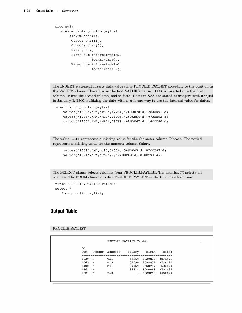
1102 Output Table 4 Chapter 34
proc sql;create table proclib.paylist
(IdNum char(4),Gender char(1),Jobcode char(3),Salary num,Birth num informat=date7.
format=date7.,Hired num informat=date7.
format=date7.);
The INSERT statement inserts data values into PROCLIB.PAYLIST according to the position inthe VALUES clause. Therefore, in the first VALUES clause, 1639 is inserted into the firstcolumn, F into the second column, and so forth. Dates in SAS are stored as integers with 0 equalto January 1, 1960. Suffixing the date with a d is one way to use the internal value for dates.
insert into proclib.paylistvalues(’1639’,’F’,’TA1’,42260,’26JUN70’d,’28JAN91’d)values(’1065’,’M’,’ME3’,38090,’26JAN54’d,’07JAN92’d)values(’1400’,’M’,’ME1’,29769.’05NOV67’d,’16OCT90’d)
The value null represents a missing value for the character column Jobcode. The periodrepresents a missing value for the numeric column Salary.
values(’1561’,’M’,null,36514,’30NOV63’d,’07OCT87’d)values(’1221’,’F’,’FA3’,.,’22SEP63’d,’04OCT94’d);
The SELECT clause selects columns from PROCLIB.PAYLIST. The asterisk (*) selects allcolumns. The FROM clause specifies PROCLIB.PAYLIST as the table to select from.
title ’PROCLIB.PAYLIST Table’;select *
from proclib.paylist;
Output Table
PROCLIB.PAYLIST
PROCLIB.PAYLIST Table 1
IdNum Gender Jobcode Salary Birth Hired-------------------------------------------------1639 F TA1 42260 26JUN70 28JAN911065 M ME3 38090 26JAN54 07JAN921400 M ME1 29769 05NOV67 16OCT901561 M 36514 30NOV63 07OCT871221 F FA3 . 22SEP63 04OCT94

The SQL Procedure 4 Program 1103
Example 2: Creating a Table from a Query’s Result
Procedure features:CREATE TABLE statement
AS query-expressionSELECT clause
column aliasFORMAT= column-modifierobject-item
Other features:data set option
OBS=
Tables:PROCLIB.PAYROLL, PROCLIB.BONUS
This example builds a column with an arithmetic expression and creates thePROCLIB.BONUS table from the query’s result.
Input Table
PROCLIB.PAYROLL (Partial Listing)
PROCLIB.PAYROLLFirst 10 Rows Only
IdNumber Sex Jobcode Salary Birth Hired------------------------------------------------1919 M TA2 34376 12SEP60 04JUN871653 F ME2 35108 15OCT64 09AUG901400 M ME1 29769 05NOV67 16OCT901350 F FA3 32886 31AUG65 29JUL901401 M TA3 38822 13DEC50 17NOV851499 M ME3 43025 26APR54 07JUN801101 M SCP 18723 06JUN62 01OCT901333 M PT2 88606 30MAR61 10FEB811402 M TA2 32615 17JAN63 02DEC901479 F TA3 38785 22DEC68 05OCT89
Program
libname proclib ’SAS-data-library’;
options nodate pageno=1 linesize=80 pagesize=40;

1104 Output 4 Chapter 34
The CREATE TABLE statement creates the table PROCLIB.BONUS from the result of thesubsequent query.
proc sql;create table proclib.bonus as
The SELECT clause specifies that three columns will be in the new table: IdNumber, Salary,and Bonus. FORMAT= assigns the DOLLAR8. format to Salary. The Bonus column is built withthe SQL expression salary*.025.
select IdNumber, Salary format=dollar8.,salary*.025 as Bonus format=dollar8.
from proclib.payroll;
The SELECT clause selects columns from PROCLIB.BONUS. The asterisk (*) selects allcolumns. The FROM clause specifies PROCLIB.BONUS as the table to select from. The OBS=data set option limits the printing of the output to 10 rows.
title ’BONUS Information’;select *
from proclib.bonus(obs=10);
Output
PROCLIB.BONUS
BONUS Information 1
IdNumber Salary Bonus--------------------------1919 $34,376 $8591653 $35,108 $8781400 $29,769 $7441350 $32,886 $8221401 $38,822 $9711499 $43,025 $1,0761101 $18,723 $4681333 $88,606 $2,2151402 $32,615 $8151479 $38,785 $970
Example 3: Updating Data in a PROC SQL TableProcedure features:
ALTER TABLE statementDROP clause

The SQL Procedure 4 Program 1105
MODIFY clauseUPDATE statement
SET clauseCASE expression
Table: EMPLOYEES
This example updates data values in the EMPLOYEES table and drops a column.
Inputdata Employees;
input IdNum $4. +2 LName $11. FName $11. JobCode $3.+1 Salary 5. +1 Phone $12.;
datalines;1876 CHIN JACK TA1 42400 212/588-56341114 GREENWALD JANICE ME3 38000 212/588-10921556 PENNINGTON MICHAEL ME1 29860 718/383-56811354 PARKER MARY FA3 65800 914/455-23371130 WOOD DEBORAH PT2 36514 212/587-0013;
Program
options nodate pageno=1 linesize=80 pagesize=40;
The SELECT clause displays the table before the updates. The asterisk (*) selects all columnsfor display.The FROM clause specifies EMPLOYEES as the table to select from.
proc sql;title ’Employees Table’;select * from Employees;
The UPDATE statement updates the values in EMPLOYEES. The SET clause specifies that thedata in the Salary column be multiplied by 1.04 when the job code ends with a 1 and 1.025 forall other job codes. (The two underscores represent any character.) The CASE expressionreturns a value for each row that completes the SET clause.
update employeesset salary=salary*case when jobcode like ’__1’ then 1.04
else 1.025end;
The ALTER TABLE statement specifies EMPLOYEES as the table to alter. The MODIFY clausepermanently modifies the format of the Salary column. The DROP clause permanently drops thePhone column.

1106 Output 4 Chapter 34
alter table employeesmodify salary num format=dollar8.drop phone;
The SELECT clause displays the EMPLOYEES table after the updates. The asterisk (*) selectsall columns.
title ’Updated Employees Table’;select * from employees;
Output
Employees Table 1
Id JobNum LName FName Code Salary Phone------------------------------------------------------------1876 CHIN JACK TA1 42400 212/588-56341114 GREENWALD JANICE ME3 38000 212/588-10921556 PENNINGTON MICHAEL ME1 29860 718/383-56811354 PARKER MARY FA3 65800 914/455-23371130 WOOD DEBORAH PT2 36514 212/587-0013
Updated Employees Table 2
Id JobNum LName FName Code Salary----------------------------------------------1876 CHIN JACK TA1 $44,0961114 GREENWALD JANICE ME3 $38,9501556 PENNINGTON MICHAEL ME1 $31,0541354 PARKER MARY FA3 $67,4451130 WOOD DEBORAH PT2 $37,427
Example 4: Joining Two Tables
Procedure features:FROM clause
table aliasinner joinjoined-table componentPROC SQL statement option
NUMBERWHERE clause
IN conditionTables: PROCLIB.STAFF, PROCLIB.PAYROLL

The SQL Procedure 4 Program 1107
This example joins two tables in order to to get more information about data that arecommon to both tables.
Input Tables
PROCLIB.STAFF (Partial Listing)
PROCLIB.STAFFFirst 10 Rows Only
IdNum Lname Fname City State Hphone----------------------------------------------------------------------------1919 ADAMS GERALD STAMFORD CT 203/781-12551653 ALIBRANDI MARIA BRIDGEPORT CT 203/675-77151400 ALHERTANI ABDULLAH NEW YORK NY 212/586-08081350 ALVAREZ MERCEDES NEW YORK NY 718/383-15491401 ALVAREZ CARLOS PATERSON NJ 201/732-87871499 BAREFOOT JOSEPH PRINCETON NJ 201/812-56651101 BAUCOM WALTER NEW YORK NY 212/586-80601333 BANADYGA JUSTIN STAMFORD CT 203/781-17771402 BLALOCK RALPH NEW YORK NY 718/384-28491479 BALLETTI MARIE NEW YORK NY 718/384-8816
PROCLIB.PAYROLL (Partial Listing)
PROCLIB.PAYROLLFirst 10 Rows Only
IdNumber Sex Jobcode Salary Birth Hired------------------------------------------------1919 M TA2 34376 12SEP60 04JUN871653 F ME2 35108 15OCT64 09AUG901400 M ME1 29769 05NOV67 16OCT901350 F FA3 32886 31AUG65 29JUL901401 M TA3 38822 13DEC50 17NOV851499 M ME3 43025 26APR54 07JUN801101 M SCP 18723 06JUN62 01OCT901333 M PT2 88606 30MAR61 10FEB811402 M TA2 32615 17JAN63 02DEC901479 F TA3 38785 22DEC68 05OCT89
Program
libname proclib ’SAS-data-library’;
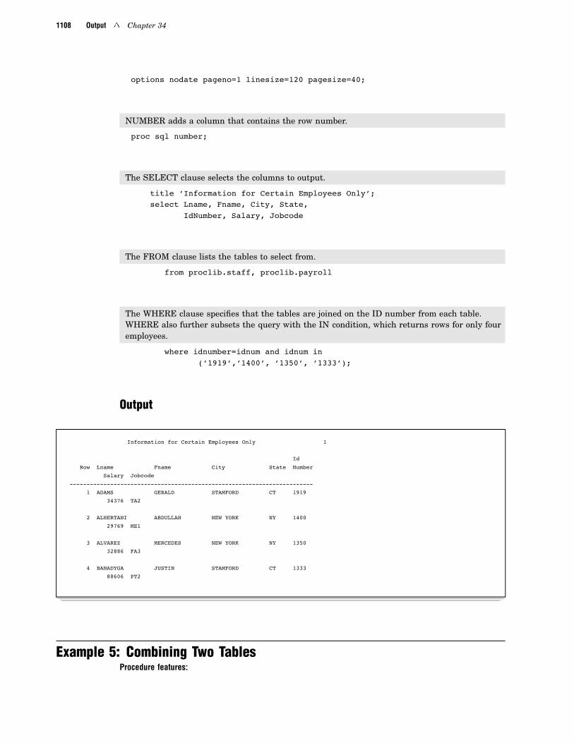
1108 Output 4 Chapter 34
options nodate pageno=1 linesize=120 pagesize=40;
NUMBER adds a column that contains the row number.
proc sql number;
The SELECT clause selects the columns to output.
title ’Information for Certain Employees Only’;select Lname, Fname, City, State,
IdNumber, Salary, Jobcode
The FROM clause lists the tables to select from.
from proclib.staff, proclib.payroll
The WHERE clause specifies that the tables are joined on the ID number from each table.WHERE also further subsets the query with the IN condition, which returns rows for only fouremployees.
where idnumber=idnum and idnum in(’1919’,’1400’, ’1350’, ’1333’);
Output
Information for Certain Employees Only 1
Id
Row Lname Fname City State Number
Salary Jobcode
------------------------------------------------------------------------
1 ADAMS GERALD STAMFORD CT 1919
34376 TA2
2 ALHERTANI ABDULLAH NEW YORK NY 1400
29769 ME1
3 ALVAREZ MERCEDES NEW YORK NY 1350
32886 FA3
4 BANADYGA JUSTIN STAMFORD CT 1333
88606 PT2
Example 5: Combining Two TablesProcedure features:

The SQL Procedure 4 Program 1109
DELETE statementIS conditionRESET statement option
DOUBLEUNION set operator
Tables: PROCLIB.NEWPAY, PROCLIB.PAYLIST, PROCLIB.PAYLIST2
This example creates a new table, PROCLIB.NEWPAY, by concatenating two othertables: PROCLIB.PAYLIST and PROCLIB.PAYLIST2.
Input Tables
PROCLIB.PAYLIST
PROCLIB.PAYLIST Table
IdNum Gender Jobcode Salary Birth Hired-------------------------------------------------1639 F TA1 42260 26JUN70 28JAN911065 M ME3 38090 26JAN54 07JAN921400 M ME1 29769 05NOV67 16OCT901561 M 36514 30NOV63 07OCT871221 F FA3 . 22SEP63 04OCT94
PROCLIB.PAYLIST2
PROCLIB.PAYLIST2 Table
IdNum Gender Jobcode Salary Birth Hired-------------------------------------------------1919 M TA2 34376 12SEP66 04JUN871653 F ME2 31896 15OCT64 09AUG921350 F FA3 36886 31AUG55 29JUL911401 M TA3 38822 13DEC55 17NOV931499 M ME1 23025 26APR74 07JUN92
Program
libname proclib ’SAS-data-library’;
options nodate pageno=1 linesize=80 pagesize=60;

1110 Output 4 Chapter 34
The SELECT clauses select all the columns from the tables listed in the FROM clauses. TheUNION set operator concatenates the query results that are produced by the two SELECTclauses. UNION orders the result by IdNum.
proc sql;create table proclib.newpay as
select * from proclib.paylistunionselect * from proclib.paylist2;
The DELETE statement deletes rows from PROCLIB.NEWPAY that satisfy the WHEREexpression. The IS condition specifies rows that contain missing values in the Jobcode or Salarycolumn.
deletefrom proclib.newpaywhere jobcode is missing or salary is missing;
RESET changes the procedure environment without stopping and restarting PROC SQL. TheDOUBLE option double-spaces the output. (The DOUBLE option has no effect on ODS output.)The SELECT clause selects all columns from the newly created table, PROCLIB.NEWPAY.
reset double;title ’Personnel Data’;select *
from proclib.newpay;
Output
Personnel Data 1
IdNum Gender Jobcode Salary Birth Hired-------------------------------------------------1065 M ME3 38090 26JAN54 07JAN92
1350 F FA3 36886 31AUG55 29JUL91
1400 M ME1 29769 05NOV67 16OCT90
1401 M TA3 38822 13DEC55 17NOV93
1499 M ME1 23025 26APR74 07JUN92
1639 F TA1 42260 26JUN70 28JAN91
1653 F ME2 31896 15OCT64 09AUG92
1919 M TA2 34376 12SEP66 04JUN87

The SQL Procedure 4 Program 1111
Example 6: Reporting from DICTIONARY Tables
Procedure features:DESCRIBE TABLE statementDICTIONARY.table-name component
Table: DICTIONARY.MEMBERS
This example uses DICTIONARY tables to show a list of the SAS files in a SAS datalibrary. If you do not know the names of the columns in the DICTIONARY table thatyou are querying, use a DESCRIBE TABLE statement with the table.
Program
libname proclib ’SAS-data-library’;
SOURCE writes the programming statements to the SAS log.
options nodate pageno=1 source linesize=80 pagesize=60;
DESCRIBE TABLE writes the column names from DICTIONARY.MEMBERS to the SAS log.
proc sql;describe table dictionary.members;
The SELECT clause selects the MEMNAME and MEMTYPE columns. The FROM clausespecifies DICTIONARY.MEMBERS as the table to select from. The WHERE clause subsets theoutput to include only those rows that have a libref of PROCLIB in the LIBNAME column.
title ’SAS Files in the PROCLIB Library’;select memname, memtype
from dictionary.memberswhere libname=’PROCLIB’;

1112 Log 4 Chapter 34
Log
2 options nodate pageno=1 source linesize=80 pagesize=60;3 proc sql;4 describe table dictionary.members;NOTE: SQL table DICTIONARY.MEMBERS was created like:
create table DICTIONARY.MEMBERS(
libname char(8) label=’Library Name’,memname char(32) label=’Member Name’,memtype char(8) label=’Member Type’,engine char(8) label=’Engine Name’,index char(32) label=’Indexes’,path char(1024) label=’Path Name’
);
5 title ’SAS Files in the PROCLIB Library’;6 select memname, memtype7 from dictionary.members8 where libname=’PROCLIB’;
Output
SAS Files in the PROCLIB Library 1
MemberMember Name Type------------------------------------------BONUS DATABONUS95 DATADELAY DATAHOUSES DATAINTERNAT DATAJOBS VIEWMARCH DATANEWPAY DATAPAYDATA VIEWPAYINFO VIEWPAYLIST DATAPAYLIST2 DATAPAYROLL DATAPAYROLL2 DATASCHEDULE DATASCHEDULE2 DATASTAFF DATASTAFF2 DATASUPERV DATASUPERV2 DATA
Example 7: Performing an Outer Join
Procedure features:joined-table componentleft outer joinSELECT clause

The SQL Procedure 4 Program 1113
COALESCE functionWHERE clause
CONTAINS conditionTables: PROCLIB.PAYROLL, PROCLIB.PAYROLL2
This example illustrates a left outer join of the PROCLIB.PAYROLL andPROCLIB.PAYROLL2 tables.
Input Tables
PROCLIB.PAYROLL (Partial Listing)
PROCLIB.PAYROLLFirst 10 Rows Only
IdNumber Sex Jobcode Salary Birth Hired------------------------------------------------1009 M TA1 28880 02MAR59 26MAR921017 M TA3 40858 28DEC57 16OCT811036 F TA3 39392 19MAY65 23OCT841037 F TA1 28558 10APR64 13SEP921038 F TA1 26533 09NOV69 23NOV911050 M ME2 35167 14JUL63 24AUG861065 M ME2 35090 26JAN44 07JAN871076 M PT1 66558 14OCT55 03OCT911094 M FA1 22268 02APR70 17APR911100 M BCK 25004 01DEC60 07MAY88
PROCLIB.PAYROLL2
PROCLIB.PAYROLL2
IdNum Sex Jobcode Salary Birth Hired----------------------------------------------1036 F TA3 42465 19MAY65 23OCT841065 M ME3 38090 26JAN44 07JAN871076 M PT1 69742 14OCT55 03OCT911106 M PT3 94039 06NOV57 16AUG841129 F ME3 36758 08DEC61 17AUG911221 F FA3 29896 22SEP67 04OCT911350 F FA3 36098 31AUG65 29JUL901369 M TA3 36598 28DEC61 13MAR871447 F FA1 22123 07AUG72 29OCT921561 M TA3 36514 30NOV63 07OCT871639 F TA3 42260 26JUN57 28JAN841998 M SCP 23100 10SEP70 02NOV92
Program

1114 Output 4 Chapter 34
libname proclib ’SAS-data-library’;
options nodate pageno=1 linesize=80 pagesize=60;
OUTOBS= limits the output to 10 rows. The SELECT clause lists the columns to select. Somecolumn names are prefixed with a table alias because they are in both tables. LABEL= andFORMAT= are column modifiers.
proc sql outobs=10;title ’Most Current Jobcode and Salary Information’;select p.IdNumber, p.Jobcode, p.Salary,
p2.jobcode label=’New Jobcode’,p2.salary label=’New Salary’ format=dollar8.
The FROM clause lists the tables to join and assigns table aliases. The keywords LEFT JOINspecify the type of join. The order of the tables in the FROM clause is important.PROCLIB.PAYROLL is listed first and is considered the "left" table, PROCLIB.PAYROLL2 isthe "right" table.
from proclib.payroll as p left join proclib.payroll2 as p2
The ON clause specifies that the join be performed based on the values of the ID numbers fromeach table.
on p.IdNumber=p2.idnum;
Output
As the output shows, all rows from the left table, PROCLIB.PAYROLL, are returned. PROCSQL assigns missing values for rows in the left table, PAYROLL, that have no matching valuesfor IdNum in PAYROLL2.
Most Current Jobcode and Salary Information 1
Id New NewNumber Jobcode Salary Jobcode Salary--------------------------------------------1009 TA1 28880 .1017 TA3 40858 .1036 TA3 39392 TA3 $42,4651037 TA1 28558 .1038 TA1 26533 .1050 ME2 35167 .1065 ME2 35090 ME3 $38,0901076 PT1 66558 PT1 $69,7421094 FA1 22268 .1100 BCK 25004 .

The SQL Procedure 4 Output 1115
The SELECT clause lists the columns to select. COALESCE overlays the like-named columns.For each row, COALESCE returns the first nonmissing value of either P2.JOBCODE orP.JOBCODE. Because P2.JOBCODE is the first argument, if there is a nonmissing value forP2.JOBCODE, COALESCE returns that value. Thus, the output contains the most recentjobcode information for every employee. LABEL= assigns a column label.
title ’Most Current Jobcode and Salary Information’;select p.idnumber, coalesce(p2.jobcode,p.jobcode)
label=’Current Jobcode’,
For each row, COALESCE returns the first nonmissing value of either P2.SALARY orP.SALARY. Because P2.SALARY is the first argument, if there is a nonmissing value forP2.SALARY, COALESCE returns that value. Thus, the output contains the most recent salaryinformation for every employee.
coalesce(p2.salary,p.salary) label=’Current Salary’format=dollar8.
The FROM clause lists the tables to join and assigns table aliases. The keywords LEFT JOINspecify the type of join. The ON clause specifies that the join is based on the ID numbers fromeach table.
from proclib.payroll p left join proclib.payroll2 p2on p.IdNumber=p2.idnum;
Output
Most Current Jobcode and Salary Information 1
Id Current CurrentNumber Jobcode Salary-------------------------1009 TA1 $28,8801017 TA3 $40,8581036 TA3 $42,4651037 TA1 $28,5581038 TA1 $26,5331050 ME2 $35,1671065 ME3 $38,0901076 PT1 $69,7421094 FA1 $22,2681100 BCK $25,004
The WHERE clause subsets the left join to include only those rows containing the value TA.
title ’Most Current Information for Ticket Agents’;select p.IdNumber,

1116 Output 4 Chapter 34
coalesce(p2.jobcode,p.jobcode) label=’Current Jobcode’,coalesce(p2.salary,p.salary) label=’Current Salary’
from proclib.payroll p left join proclib.payroll2 p2on p.IdNumber=p2.idnumwhere p2.jobcode contains ’TA’;
Output
Most Current Information for Ticket Agents 1
Id Current CurrentNumber Jobcode Salary-------------------------1036 TA3 424651369 TA3 365981561 TA3 365141639 TA3 42260
Example 8: Creating a View from a Query’s Result
Procedure features:CREATE VIEW statementGROUP BY clauseSELECT clause
COUNT functionHAVING clause
Other features:AVG summary functiondata set option
PW=Tables: PROCLIB.PAYROLL, PROCLIB.JOBS
This example creates the PROC SQL view PROCLIB.JOBS from the result of aquery-expression.
Input Table

The SQL Procedure 4 Program 1117
PROCLIB.PAYROLL (Partial Listing)
PROCLIB.PAYROLLFirst 10 Rows Only
IdNumber Sex Jobcode Salary Birth Hired------------------------------------------------1009 M TA1 28880 02MAR59 26MAR921017 M TA3 40858 28DEC57 16OCT811036 F TA3 39392 19MAY65 23OCT841037 F TA1 28558 10APR64 13SEP921038 F TA1 26533 09NOV69 23NOV911050 M ME2 35167 14JUL63 24AUG861065 M ME2 35090 26JAN44 07JAN871076 M PT1 66558 14OCT55 03OCT911094 M FA1 22268 02APR70 17APR911100 M BCK 25004 01DEC60 07MAY88
Program
libname proclib ’SAS-data-library’;
options nodate pageno=1 linesize=80 pagesize=60;
CREATE VIEW creates the PROC SQL view PROCLIB.JOBS. The PW= data set option assignspassword protection to the data generated by this view.
proc sql;create view proclib.jobs(pw=red) as
The SELECT clause specifies four columns for the view: Jobcode and three columns, Number,AVGAGE, and AVGSAL, whose values are the products of functions. COUNT returns thenumber of nonmissing values for each jobcode because the data are grouped by Jobcode.LABEL= assigns a label to the column.
select Jobcode,count(jobcode) as number label=’Number’,
The AVG summary function calculates the average age and average salary for each jobcode.
avg(int((today()-birth)/365.25)) as avgageformat=2. label=’Average Age’,
avg(salary) as avgsalformat=dollar8. label=’Average Salary’
The FROM clause specifies PAYROLL as the table to select from. PROC SQL assumes the librefof PAYROLL to be PROCLIB because PROCLIB is used in the CREATE VIEW statement.

1118 Output 4 Chapter 34
from payroll
The GROUP BY clause groups the data by the values of Jobcode. Thus, any summary statisticsare calculated for each grouping of rows by value of Jobcode. The HAVING clause subsets thegrouped data and returns rows for job codes that contain an average age of greater than orequal to 30.
group by jobcodehaving avgage ge 30;
The SELECT statement selects all columns from PROCLIB.JOBS. PW=RED is necessarybecause the view is password-protected.
title ’Current Summary Information for Each Job Category’;title2 ’Average Age Greater Than Or Equal to 30’;select * from proclib.jobs(pw=red);
Output
Current Summary Information for Each Job Category 1Average Age Greater Than Or Equal to 30
Average AverageJobcode Number Age Salary------------------------------------BCK 9 33 $25,794FA2 16 34 $27,987FA3 7 35 $32,934ME1 8 30 $28,500ME2 14 36 $35,577ME3 7 39 $42,411NA2 3 38 $52,383PT1 8 34 $67,908PT2 10 39 $87,925PT3 2 50 $10,505SCP 7 34 $18,309TA1 9 32 $27,721TA2 20 33 $33,575TA3 12 37 $39,680
Example 9: Joining Three Tables
Procedure features:FROM clausejoined-table componentWHERE clause
Tables: PROCLIB.STAFF2, PROCLIB.SCHEDULE2, PROCLIB.SUPERV2

The SQL Procedure 4 Input Tables 1119
This example joins three tables and produces a report that contains columns fromeach table.
Input Tables
PROCLIB.STAFF2
PROCLIB.STAFF2
IdNum Lname Fname City State Hphone----------------------------------------------------------------------------1106 MARSHBURN JASPER STAMFORD CT 203/781-14571430 DABROWSKI SANDRA BRIDGEPORT CT 203/675-16471118 DENNIS ROGER NEW YORK NY 718/383-11221126 KIMANI ANNE NEW YORK NY 212/586-12291402 BLALOCK RALPH NEW YORK NY 718/384-28491882 TUCKER ALAN NEW YORK NY 718/384-02161479 BALLETTI MARIE NEW YORK NY 718/384-88161420 ROUSE JEREMY PATERSON NJ 201/732-98341403 BOWDEN EARL BRIDGEPORT CT 203/675-34341616 FUENTAS CARLA NEW YORK NY 718/384-3329
PROCLIB.SCHEDULE2
PROCLIB.SCHEDULE2
IdFlight Date Dest Num---------------------------132 01MAR94 BOS 1118132 01MAR94 BOS 1402219 02MAR94 PAR 1616219 02MAR94 PAR 1478622 03MAR94 LON 1430622 03MAR94 LON 1882271 04MAR94 NYC 1430271 04MAR94 NYC 1118579 05MAR94 RDU 1126579 05MAR94 RDU 1106

1120 Program 4 Chapter 34
PROCLIB.SUPERV2
PROCLIB.SUPERV2
Supervisor JobId State Category---------------------------1417 NJ NA1352 NY NA1106 CT PT1442 NJ PT1118 NY PT1405 NJ SC1564 NY SC1639 CT TA1126 NY TA1882 NY ME
Program
libname proclib ’SAS-data-library’;
options nodate pageno=1 linesize=80 pagesize=60;
The SELECT clause specifies the columns to select. IdNum is prefixed with a table alias becauseit appears in two tables.
proc sql;title ’All Flights for Each Supervisor’;
select s.IdNum, Lname, City ’Hometown’, Jobcat,Flight, Date
The FROM clause lists the three tables for the join and assigns an alias to each table.
from proclib.schedule2 s, proclib.staff2 t, proclib.superv2 v
The WHERE clause specifies the columns that join the tables. The STAFF2 and SCHEDULE2tables have an IdNum column, which has related values in both tables. The STAFF2 andSUPERV2 tables have the IdNum and SUPID columns, which have related values in both tables.
where s.idnum=t.idnum and t.idnum=v.supid;

The SQL Procedure 4 Program 1121
Output
All Flights for Each Supervisor 1
Id JobNum Lname Hometown Category Flight Date-----------------------------------------------------------------1106 MARSHBURN STAMFORD PT 579 05MAR941118 DENNIS NEW YORK PT 132 01MAR941118 DENNIS NEW YORK PT 271 04MAR941126 KIMANI NEW YORK TA 579 05MAR941882 TUCKER NEW YORK ME 622 03MAR94
Example 10: Querying an In-Line ViewProcedure features:
FROM clausein-line view
Tables: PROCLIB.STAFF, PROCLIB.SCHEDULE, PROCLIB.SUPERV
This example uses the query explained in Example 9 on page 1118 as an in-line view.The example also shows how to rename columns with an in-line view.
Program
libname proclib ’SAS-data-library’;
options nodate pageno=1 linesize=80 pagesize=60;
The SELECT clause selects all columns returned by the query in the FROM clause.
proc sql outobs=10;title ’All Flights for Each Supervisor’;select *
The query that joins the three tables is used in the FROM clause instead of the name of a tableor view. In the in-line query, the SELECT clause lists the columns to select. IdNum is prefixedwith a table alias because it appears in two tables. The FROM clause lists the three tables forthe join and assigns an alias to each table. The WHERE clause specifies the columns that jointhe tables. The STAFF2 and SCHEDULE2 tables have an IdNum column, which has relatedvalues in both tables. The STAFF2 and SUPERV2 tables have the IdNum and SUPID columns,which have related values in both tables.
from (select lname, s.idnum, city, jobcat,flight, date

1122 Output 4 Chapter 34
from proclib.schedule2 s, proclib.staff2 t,proclib.superv2 v
where s.idnum=t.idnum and t.idnum=v.supid)
The alias THREE refers to the entire query. The names in parentheses become the names forthe columns in the output. The label Job Category appears in the output instead of the nameJobtype because PROC SQL prints a column’s label if the column has a label.
as three (Surname, Emp_ID, Hometown,Jobtype, FlightNumber, FlightDate);
Output
All Flights for Each Supervisor 1
JobSurname Emp_ID Hometown Category FlightNumber FlightDate----------------------------------------------------------------------------MARSHBURN 1106 STAMFORD PT 579 05MAR94DENNIS 1118 NEW YORK PT 132 01MAR94DENNIS 1118 NEW YORK PT 271 04MAR94KIMANI 1126 NEW YORK TA 579 05MAR94TUCKER 1882 NEW YORK ME 622 03MAR94
Example 11: Retrieving Values with the SOUNDS-LIKE Operator
Procedure features:ORDER BY clauseSOUNDS-LIKE operator
Table: PROCLIB.STAFF
This example returns rows based on the functionality of the SOUNDS-LIKE operatorin a WHERE clause.
Input Table

The SQL Procedure 4 Output 1123
PROCLIB.STAFF
PROCLIB.STAFFFirst 10 Rows Only
IdNum Lname Fname City State Hphone----------------------------------------------------------------------------1919 ADAMS GERALD STAMFORD CT 203/781-12551653 ALIBRANDI MARIA BRIDGEPORT CT 203/675-77151400 ALHERTANI ABDULLAH NEW YORK NY 212/586-08081350 ALVAREZ MERCEDES NEW YORK NY 718/383-15491401 ALVAREZ CARLOS PATERSON NJ 201/732-87871499 BAREFOOT JOSEPH PRINCETON NJ 201/812-56651101 BAUCOM WALTER NEW YORK NY 212/586-80601333 BANADYGA JUSTIN STAMFORD CT 203/781-17771402 BLALOCK RALPH NEW YORK NY 718/384-28491479 BALLETTI MARIE NEW YORK NY 718/384-8816
Program
libname proclib ’SAS-data-library’;
options nodate pageno=1 linesize=80 pagesize=60;
The SELECT clause selects all columns from the table in the FROM clause, PROCLIB.STAFF.
proc sql;title "Employees Whose Last Name Sounds Like ’Johnson’";select *
from proclib.staff
The WHERE clause uses the SOUNDS-LIKE operator to subset the table by those employeeswhose last name sounds like Johnson. The ORDER BY clause orders the output by the secondcolumn.
where lname=*"Johnson"order by 2;
Output
Employees Whose Last Name Sounds Like ’Johnson’ 1
IdNum Lname Fname City State Hphone----------------------------------------------------------------------------1411 JOHNSEN JACK PATERSON NJ 201/732-36781113 JOHNSON LESLIE NEW YORK NY 718/383-30031369 JONSON ANTHONY NEW YORK NY 212/587-5385

1124 Example 12: Joining Two Tables and Calculating a New Value 4 Chapter 34
SOUNDS-LIKE is useful, but there may be instances where it does not return every row thatseems to satisfy the condition. PROCLIB.STAFF has an employee with the last name SANDERSand an employee with the last name SANYERS. The algorithm does not find SANYERS, but itdoes find SANDERS and SANDERSON.
title "Employees Whose Last Name Sounds Like ’Sanders’";select *
from proclib.staffwhere lname=*"Sanders"order by 2;
Employees Whose Last Name Sounds Like ’Sanders’ 2
IdNum Lname Fname City State Hphone----------------------------------------------------------------------------1561 SANDERS RAYMOND NEW YORK NY 212/588-66151414 SANDERSON NATHAN BRIDGEPORT CT 203/675-17151434 SANDERSON EDITH STAMFORD CT 203/781-1333
Example 12: Joining Two Tables and Calculating a New ValueProcedure features:
GROUP BY clauseHAVING clauseSELECT clause
ABS functionFORMAT= column-modifierLABEL= column-modifierMIN summary function** operator, exponentiationSQRT function
Tables: STORES, HOUSES
This example joins two tables in order to compare and analyze values that are uniqueto each table yet have a relationship with a column that is common to both tables.
options ls=80 ps=60 nodate pageno=1 ;data stores;
input Store $ x y;datalines;
store1 6 1store2 5 2store3 3 5store4 7 5

The SQL Procedure 4 Program 1125
;data houses;
input House $ x y;datalines;
house1 1 1house2 3 3house3 2 3house4 7 7;
Input Tables
STORES and HOUSES
The tables contain X and Y coordinates that represent the location of the stores and houses.
STORES Table 1Coordinates of Stores
Store x y----------------------------store1 6 1store2 5 2store3 3 5store4 7 5
HOUSES Table 2Coordinates of Houses
House x y----------------------------house1 1 1house2 3 3house3 2 3house4 7 7
Program
options nodate pageno=1 linesize=80 pagesize=60;
The SELECT clause specifies three columns: HOUSE, STORE, and DIST. The arithmeticexpression uses the square root function (SQRT) to create the values of DIST, which contain thedistance from HOUSE to STORE for each row. The double asterisk (**) representsexponentiation. LABEL= assigns a label to STORE and to DIST.
proc sql;title ’Each House and the Closest Store’;select house, store label=’Closest Store’,
sqrt((abs(s.x-h.x)**2)+(abs(h.y-s.y)**2)) as dist
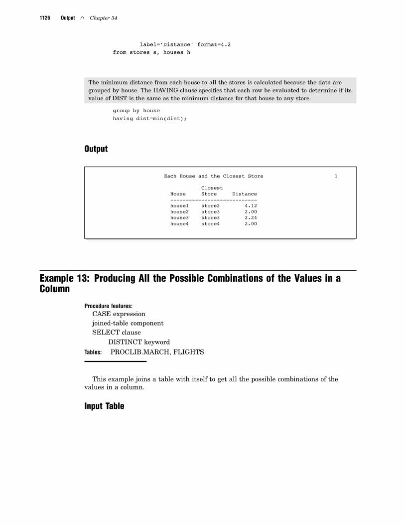
1126 Output 4 Chapter 34
label=’Distance’ format=4.2from stores s, houses h
The minimum distance from each house to all the stores is calculated because the data aregrouped by house. The HAVING clause specifies that each row be evaluated to determine if itsvalue of DIST is the same as the minimum distance for that house to any store.
group by househaving dist=min(dist);
Output
Each House and the Closest Store 1
ClosestHouse Store Distance----------------------------house1 store2 4.12house2 store3 2.00house3 store3 2.24house4 store4 2.00
Example 13: Producing All the Possible Combinations of the Values in aColumn
Procedure features:CASE expressionjoined-table componentSELECT clause
DISTINCT keywordTables: PROCLIB.MARCH, FLIGHTS
This example joins a table with itself to get all the possible combinations of thevalues in a column.
Input Table

The SQL Procedure 4 Output 1127
PROCLIB.MARCH (Partial Listing)
PROCLIB.MARCHFirst 10 Rows Only
Flight Date Depart Orig Dest Miles Boarded Capacity-----------------------------------------------------------------114 01MAR94 7:10 LGA LAX 2475 172 210202 01MAR94 10:43 LGA ORD 740 151 210219 01MAR94 9:31 LGA LON 3442 198 250622 01MAR94 12:19 LGA FRA 3857 207 250132 01MAR94 15:35 LGA YYZ 366 115 178271 01MAR94 13:17 LGA PAR 3635 138 250302 01MAR94 20:22 LGA WAS 229 105 180114 02MAR94 7:10 LGA LAX 2475 119 210202 02MAR94 10:43 LGA ORD 740 120 210219 02MAR94 9:31 LGA LON 3442 147 250
Program
libname proclib ’SAS-data-library’;
options nodate pageno=1 linesize=80 pagesize=60;
The CREATE TABLE statement creates the table FLIGHTS from the output of the query. TheSELECT clause selects the unique values of Dest. DISTINCT specifies that only one row foreach value of city be returned by the query and stored in the table FLIGHTS. The FROM clausespecifies PROCLIB.MARCH as the table to select from.
proc sql;create table flights as
select distinct destfrom proclib.march;
title ’Cities Serviced by the Airline’;
select * from flights;
Output

1128 Output 4 Chapter 34
FLIGHTS Table
Cities Serviced by the Airline 1
Dest----FRALAXLONORDPARWASYYZ
The SELECT clause specifies three columns for the output. The prefixes on DEST are tablealiases to specify which table to take the values of Dest from. The CASE expression creates acolumn that contains the character string to and from.
title ’All Possible Connections’;select f1.Dest, case
when f1.dest ne ’ ’ then ’to and from’end,
f2.Dest
The FROM clause joins FLIGHTS with itself and creates a table that contains every possiblecombination of rows. The table contains two rows for each possible route, for example,PAR <-> WAS and WAS <-> PAR.
from flights as f1, flights as f2
The WHERE clause subsets the internal table by choosing only those rows where the name inF1.Dest sorts before the name in F2.Dest. Thus, there is only one row for each possible route.
where f1.dest < f2.dest
ORDER BY sorts the result by the values of F1.Dest.
order by f1.dest;
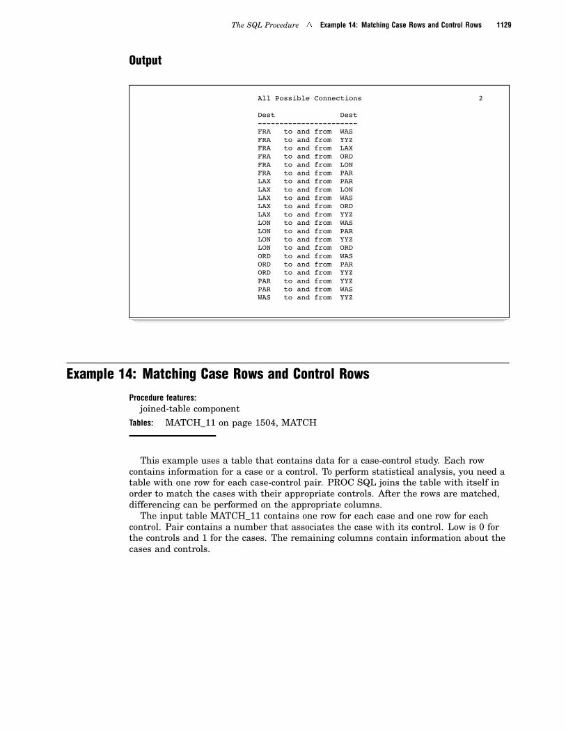
The SQL Procedure 4 Example 14: Matching Case Rows and Control Rows 1129
Output
All Possible Connections 2
Dest Dest-----------------------FRA to and from WASFRA to and from YYZFRA to and from LAXFRA to and from ORDFRA to and from LONFRA to and from PARLAX to and from PARLAX to and from LONLAX to and from WASLAX to and from ORDLAX to and from YYZLON to and from WASLON to and from PARLON to and from YYZLON to and from ORDORD to and from WASORD to and from PARORD to and from YYZPAR to and from YYZPAR to and from WASWAS to and from YYZ
Example 14: Matching Case Rows and Control Rows
Procedure features:joined-table component
Tables: MATCH_11 on page 1504, MATCH
This example uses a table that contains data for a case-control study. Each rowcontains information for a case or a control. To perform statistical analysis, you need atable with one row for each case-control pair. PROC SQL joins the table with itself inorder to match the cases with their appropriate controls. After the rows are matched,differencing can be performed on the appropriate columns.
The input table MATCH_11 contains one row for each case and one row for eachcontrol. Pair contains a number that associates the case with its control. Low is 0 forthe controls and 1 for the cases. The remaining columns contain information about thecases and controls.

1130 Input Table 4 Chapter 34
Input Table
MATCH_11 Table
First 10 Rows Only
Pair Low Age Lwt Race Smoke Ptd Ht UI race1 race2
------------------------------------------------------------------------------------------------------------
1 0 14 135 1 0 0 0 0 0 0
1 1 14 101 3 1 1 0 0 0 1
2 0 15 98 2 0 0 0 0 1 0
2 1 15 115 3 0 0 0 1 0 1
3 0 16 95 3 0 0 0 0 0 1
3 1 16 130 3 0 0 0 0 0 1
4 0 17 103 3 0 0 0 0 0 1
4 1 17 130 3 1 1 0 1 0 1
5 0 17 122 1 1 0 0 0 0 0
5 1 17 110 1 1 0 0 0 0 0
Program
options nodate pageno=1 linesize=80 pagesize=60;
The SELECT clause specifies the columns for the table MATCH. SQL expressions in theSELECT clause calculate the differences for the appropriate columns and create new columns.
proc sql;create table match as
selectone.Low,one.Pair,(one.lwt - two.lwt) as Lwt_d,(one.smoke - two.smoke) as Smoke_d,(one.ptd - two.ptd) as Ptd_d,(one.ht - two.ht) as Ht_d,(one.ui - two.ui) as UI_d
The FROM clause lists the table MATCH_11 twice. Thus, the table is joined with itself. TheWHERE clause returns only the rows for each pair that show the difference when the values forcontrol are subtracted from the values for case.
from match_11 one, match_11 twowhere (one.pair=two.pair and one.low>two.low);
The SELECT clause selects all the columns from MATCH. The OBS= data set option limits theprinting of the output to five rows.
title ’Differences for Cases and Controls’;select *
from match(obs=5);

The SQL Procedure 4 Program 1131
Output
MATCH Table
Differences for Cases and Controls 1
Low Pair Lwt_d Smoke_d Ptd_d Ht_d UI_d--------------------------------------------------------------------
1 1 -34 1 1 0 01 2 17 0 0 0 11 3 35 0 0 0 01 4 27 1 1 0 11 5 -12 0 0 0 0
Example 15: Counting Missing Values with a SAS MacroProcedure feature:
COUNT functionTable: SURVEY
This example uses a SAS macro to create columns. The SAS macro is not explainedhere. See the SAS Guide to Macro Processing for complete documentation on the SASCOUNTM macro.
Input Table
SURVEY contains data from a questionnaire about diet and exercise habits. SAS enables you touse a special notation for missing values. In the EDUC column, the .x notation indicates thatthe respondent gave an answer that is not valid, and .n indicates that the respondent did notanswer the question. A period as a missing value indicates a data entry error.
data survey;input id $ diet $ exer $ hours xwk educ;datalines;
1001 yes yes 1 3 11002 no yes 1 4 21003 no no . . .n1004 yes yes 2 3 .x1005 no yes 2 3 .x1006 yes yes 2 4 .x1007 no yes .5 3 .1008 no no . . .;
Program

1132 Program 4 Chapter 34
options nodate pageno=1 linesize=80 pagesize=60;
The COUNTM macro uses the COUNT function to perform various counts for a column. EachCOUNT function uses a CASE expression to select the rows to be counted. The first COUNTfunction uses only the column as an argument to return the number of nonmissing rows.
%macro countm(col);count(&col) "Valid Responses for &col",
The IS MISSING keywords return the rows that have any type of missing value: .n, .x, or aperiod. The PUT function returns a character string to be counted.
count(casewhen &col is missing then put(&col, 2.)end) "Missing or NOT VALID Responses for &col",
The last three COUNT functions use CASE expressions to count the occurrences of the threenotations for missing values.
count(casewhen &col=.n then put(&col, 2.)end) "Coded as NO ANSWER for &col",
count(casewhen &col=.x then put(&col, 2.)end) "Coded as NOT VALID answers for &col",
count(casewhen &col=. then put(&col, 1.)end) "Data Entry Errors for &col"
%mend;
The SELECT clause specifies the columns that are in the output. COUNT(*) returns the totalnumber of rows in the table. The COUNTM macro uses the values of the EDUC column tocreate the columns defined in the macro.
proc sql;title ’Counts for Each Type of Missing Response’;select count(*) "Total No. of Rows",
%countm(educ)from survey;

The SQL Procedure 4 Output 1133
Output
Counts for Each Type of Missing Response 1
Missing Coded asor NOT Coded as NOT Data
Total Valid VALID NO VALID EntryNo. of Responses Responses ANSWER answers Errors
Rows for educ for educ for educ for educ for educ------------------------------------------------------------
8 2 6 1 3 2

1134 Output 4 Chapter 34

The correct bibliographic citation for this manual is as follows: SAS Institute Inc., SAS ®
Procedures Guide, Version 8, Cary, NC: SAS Institute Inc., 1999. 1729 pp.
SAS® Procedures Guide, Version 8Copyright © 1999 by SAS Institute Inc., Cary, NC, USA.ISBN 1–58025–482–9All rights reserved. Printed in the United States of America. No part of this publicationmay be reproduced, stored in a retrieval system, or transmitted, in any form or by anymeans, electronic, mechanical, photocopying, or otherwise, without the prior writtenpermission of the publisher, SAS Institute Inc.U.S. Government Restricted Rights Notice. Use, duplication, or disclosure of thesoftware and related documentation by the U.S. government is subject to the Agreementwith SAS Institute and the restrictions set forth in FAR 52.227–19 Commercial ComputerSoftware-Restricted Rights (June 1987).SAS Institute Inc., SAS Campus Drive, Cary, North Carolina 27513.1st printing, October 1999SAS® and all other SAS Institute Inc. product or service names are registered trademarksor trademarks of SAS Institute Inc. in the USA and other countries.® indicates USAregistration.IBM® and DB2® are registered trademarks or trademarks of International BusinessMachines Corporation. ORACLE® is a registered trademark of Oracle Corporation. ®
indicates USA registration.Other brand and product names are registered trademarks or trademarks of theirrespective companies.The Institute is a private company devoted to the support and further development of itssoftware and related services.