Ple

ase

note

that

this

is a

n au

thor

-pro

duce

d P

DF

of a

n ar

ticle

acc

ept

ed fo

r pu

blic

atio

n fo

llow

ing

peer

rev

iew

. The

def

initi

ve p

ub

lish

er-a

uthe

ntic

ated

ve

rsio

n is

ava

ilab

le o

n th

e pu

blis

her

Web

site

1

International Journal of Adhesion and Adhesives October 2009, Volume 29, Issue 7, Pages 724-736 http://dx.doi.org/10.1016/j.ijadhadh.2009.03.002 © 2009 Elsevier Ltd All rights reserved.

Archimer Archive Institutionnelle de l’Ifremer

http://www.ifremer.fr/docelec/

Influence of adhesive bond line thickness on joint strength

P. Daviesa, *, L. Sohierb, J.-Y. Cognardc, A. Bourmaudd, D. Choqueusea, E. Rinnerte and R. Créac’hcadecb, c

a Materials and Structures group, IFREMER Brest Centre, 29280 Plouzané, France b LBMS, Université de Bretagne Occidentale, 29285 Brest, France c LBMS, ENSIETA, 29806 Brest, France d L2PIC, Université de Bretagne Sud, 56321 Lorient, France e Interfaces Group, IFREMER Brest Centre, 29280 Plouzané, France *: Corresponding author : Davies P., Tel.: +33 298 22 4777; fax: +33 298 22 4535, email address : Peter.Davies@ifremer.fr

Abstract: While the geometry of aerospace assemblies is carefully controlled, for many industrial applications such as marine structures bond line thickness can vary significantly. In this study epoxy adhesive joints of different thicknesses between aluminium substrates have been characterized using physico-chemical analyses (differential scanning calorimetry, DSC; dynamic mechanical analysis, DMA; spectroscopy), nano-indentation and mechanical testing. Thermal analyses indicated no influence of thickness on structure. Nano-indentation revealed no evidence of an interphase at the metal/epoxy interface, nor any change in modulus for different thicknesses, though Raman spectroscopy suggested there may be slight variations in composition close to the substrates. However, mechanical testing using the modified Arcan fixture indicated a significant drop in strength and failure strain under pure tension and a smaller reduction for tension/shear and pure shear loads as thickness increased. Examination of sections through joints did not indicate any physical reason for this, but numerical analysis of the stress state revealed larger stress concentration factors for tensile loading in thick joints, which may explain the thickness effect. It is recommended that joint thickness should be kept below 0.8 mm to avoid obtaining artificially low values with the Arcan test. Keywords: Epoxy; Aluminium; Mechanical properties; Arcan

2 04/03/2009

1. Introduction

Adhesive bonding is now an established joining method which has been reviewed in detail

recently [1]. It is a particularly attractive assembly technique for applications where weight

gain is at a premium, and racing yachts are one such example. However, the large scale of

structures such as boat hulls results in significant dimensional variations, so that it is not

possible to achieve the thin bond lines and tight tolerances imposed in bonded aerospace

structures. It is therefore essential to be able to characterize the influence of this parameter,

and this was the aim of the present study. There have been several previous studies in this

area using two approaches, based on either fracture mechanics or stress analysis. Kinloch [2]

reviewed some early studies of both types. For lap shear specimens, the simple stress analyses

for this geometry indicate a strong increase in failure stress with increasing joint thickness

while measurements and finite element analysis indicate much lower sensitivity to this

parameter [3]. In early studies on bond line thickness Bascom and colleagues [4] and then

Kinloch & Shaw [5] used linear elastic fracture mechanics tests to characterize the crack

propagation resistance of joints up to 3mm thick. They found an optimum joint thickness

around 0.5mm, and postulated that there is competition between a constraint mechanism, due

to the rigid substrates, at low thickness, resulting in high tensile stresses, and the amount of

dissipation in the plastic zone which increases to a maximum then reduces at higher thickness.

The following expression was proposed for the optimal joint thickness h, based on the fully

developed plastic zone radius (rp), for plane stress and linear elastic fracture mechanics [5]:

== 2

12

y

cp

EGrh

σπ (1)

where E is the adhesive modulus, Gc the critical strain energy release rate and σy the yield

stress. A peak in toughness versus bond line thickness can be expected when rp equals the

latter. These results were cited by Kinloch & Moore [6], who presented further data which

showed the same trend. More recently Kawashita et al. presented peel test data from

aluminium joints with bond line thicknesses of 0.1, 0.25 and 0.4 mm, below the optimal

thickness, for two epoxy adhesives [7]. Measured toughness increased with thickness and a

reasonable fit was obtained between test results and their LEFM model. Mall and

Ramamurthy used double cantilever beam specimens to examine fracture and crack growth

under cyclic loading in joints of different thicknesses [8]. DCB joints with different adhesive

thickness showed similar thresholds at lower crack growth rates, whereas a thicker adhesive

layer resulted in an improved resistance to the crack growth for high propagation rates. Gleich

3 04/03/2009

et al. also used a fracture mechanics approach, to show that the stress intensity factors, after

an initial decrease in the low bondline thickness range, increased with increasing bondline

thickness [9]. In another study, using the more traditional stress-based approach, Tomblin et

al [10] presented results from thick adherend shear test (TAST) and thin adherend lap shear

specimens with adhesive thicknesses in a wide range from 0.4 to 3 mm. Their aim was to

produce stress-strain data for design of secondary bonded assemblies in general aviation

applications, for which joints may be thicker than the previously-standard 0.25mm thickness.

They noted a decrease in apparent shear strength with increasing joint thickness for the three

adhesives tested on aluminium substrates with both tests. TAST specimens gave consistently

higher values than thin adherend lap shear specimens at all bond line thicknesses, due to the

development of peel stresses in the latter. Grant et al also presented results from tests on lap

shear specimens which showed a linear drop in failure load as bond-line thickness was

increased from 0.1 to 3 mm, and they attributed this to an increase in bending stress for the

thicker adhesives [11]. Taib et al recently showed results for L-section joints with adhesive

thicknesses of 0.127, 0.635 and 2.54 mm [12]. Failure loads dropped from 8.27 to 3.9 kN as

joint thickness increased, and this was attributed to a change from plane stress to plane strain

states. Finally, Jarry & Shenoi examined 1, 5 and 10mm butt strap metallic assemblies bonded

with a methacrylate adhesive and found similar strengths for 1 and 5mm but significantly

lower values for the thickest bond-line [13].

This summary of some of the previous work on bond line thickness, and the fact that

many of the papers cited are very recent, underlines the importance of this subject. There is a

tendency for measured failure stress to decrease with increasing bondline thickness, but

interpreting variations in properties can be quite complex as various factors may intervene to

modify the behaviour of joints as their thickness is increased:

- First, the nature or dimensions of defects may vary with bond line thickness.

Visual and microscopic examination can be used to check this effect.

- Second, the adhesive structure may change as thickness increases. This may

be caused by differences in cure conditions for example. Heterogeneous

thermal behaviour, such as exotherm dissipation, will depend on the

proximity of conductive substrates. Thermal analyses or local property

measurements may enable such variations to be detected.

- Thirdly, the adhesive/substrate interface properties may be modified as

thickness increases. This may be due to internal stresses developing at this

interface [14], to migration of species from the substrates into the adhesive

4 04/03/2009

(oxides) or to changes of stoichiometry within the adhesive near the substrate.

Roche and colleagues have examined these phenomena in detail [15]. Many

techniques have been used to detect interphases, based on changes in

chemical state (by Infra-Red spectroscopy or micro-thermal analysis for

example [16]) or mechanical properties (tensile, nano-indentation or even

laser acoustic methods [17]).

- Fourthly, the energy dissipating mechanisms (plasticity, damage

development) may be modified by changing the distance between the

substrates. Careful mechanical testing can be used to illustrate this.

- Finally, the change in specimen geometry with increasing bond line thickness

may cause a change in the stress state within the joint so that tests on

specimens with different thicknesses are not measuring the same properties.

In order to examine this detailed stress analysis of the joint is required.

In the present paper these different factors will be examined using various techniques, in order

to conclude on the influence of joint thickness on the mechanical behaviour of aluminium

substrates bonded with a tough epoxy adhesive. Here we focus mainly on the non-linear

behaviour of the adhesive rather than crack propagation.

2. Materials

The adhesive examined here is a two-part system. 100 parts by weight of a DGEBA

(diglicidyl ether of bisphenol A) epoxy pre-polymer are mixed with 40 parts of TTD

(trioxatridecane diamine) hardener, previously marketed as Redux 420, now Araldite 420

supplied by Huntsman. This adhesive has been widely-used for many years, in both the

aerospace and marine industries. It contains some spherical fillers, estimated from burn-off to

represent around 8% by weight. EDX (Energy Dispersive X-ray) analysis in the electron

microscope indicated these to be solid glass spheres as will be described below. The choice of

a commercial adhesive for this study, rather than a model epoxy, was made so that the results

would be of direct interest for industrial assemblies. However, the complex formulation does

make interpretation of results more complicated. The substrates are aluminium 2017 grade

alloy.

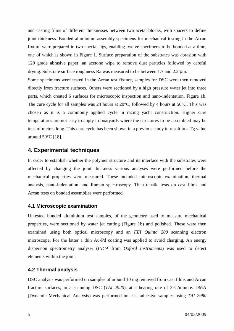
3. Specimen preparation

Adhesive film samples, for DSC (Differential Scanning Calorimetry), DMA (Dynamic

Mechanical Analysis), and tensile tests, were produced by mixing the adhesive and hardener

5 04/03/2009

and casting films of different thicknesses between two acetal blocks, with spacers to define

joint thickness. Bonded aluminium assembly specimens for mechanical testing in the Arcan

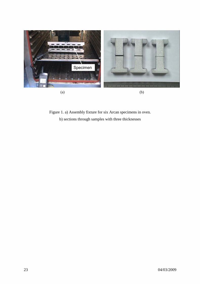
fixture were prepared in two special jigs, enabling twelve specimens to be bonded at a time,

one of which is shown in Figure 1. Surface preparation of the substrates was abrasion with

120 grade abrasive paper, an acetone wipe to remove dust particles followed by careful

drying. Substrate surface roughness Ra was measured to be between 1.7 and 2.2 µm.

Some specimens were tested in the Arcan test fixture, samples for DSC were then removed

directly from fracture surfaces. Others were sectioned by a high pressure water jet into three

parts, which created 6 surfaces for microscopic inspection and nano-indentation, Figure 1b.

The cure cycle for all samples was 24 hours at 20°C, followed by 4 hours at 50°C. This was

chosen as it is a commonly applied cycle in racing yacht construction. Higher cure

temperatures are not easy to apply in boatyards where the structures to be assembled may be

tens of metres long. This cure cycle has been shown in a previous study to result in a Tg value

around 50°C [18].

4. Experimental techniques

In order to establish whether the polymer structure and its interface with the substrates were

affected by changing the joint thickness various analyses were performed before the

mechanical properties were measured. These included microscopic examination, thermal

analysis, nano-indentation, and Raman spectroscopy. Then tensile tests on cast films and

Arcan tests on bonded assemblies were performed.

4.1 Microscopic examination

Untested bonded aluminium test samples, of the geometry used to measure mechanical

properties, were sectioned by water jet cutting (Figure 1b) and polished. These were then

examined using both optical microscopy and an FEI Quinta 200 scanning electron

microscope. For the latter a thin Au-Pd coating was applied to avoid charging. An energy

dispersion spectrometry analyser (INCA from Oxford Instruments) was used to detect

elements within the joint.

4.2 Thermal analysis

DSC analysis was performed on samples of around 10 mg removed from cast films and Arcan

fracture surfaces, in a scanning DSC (TAI 2920), at a heating rate of 3°C/minute. DMA

(Dynamic Mechanical Analysis) was performed on cast adhesive samples using TAI 2980

6 04/03/2009

equipment in the tension mode at a frequency of 1 Hz, on 10mm wide, 35mm long film

samples clamped at both ends. These were also heated at 3°C/minute, from 20 to 120°C.

4.3 Nano-indentation

Depth sensing indentation (DSI), often referred to as nanoindentation is a powerful technique

enabling local variations in modulus to be measured [19]. Many authors have investigated

interphase regions in various materials by using nanoindentation. For example, Zhu et al. [20]

studied modulus and hardness of PVC/rubber blends using nanoindentation. They have shown

an interface region characterized by an abrupt change in modulus and hardness. Bourmaud et

al [21] investigated nanomechanical characteristics of recycled poly(carbonate)/crushed

rubber blends by using nanoindentation. They revealed an interphase region between the

matrix and the rubber particles. Lee et al [22] have used nanoindentation to evaluate

interphase properties of a cellulose fiber–reinforced polypropylene composite; hardness and

modulus in the transition region were used to charecterise its mechanical properties. Ureña et

al. [23, 24] carried out nanoindentation in order to determine interfacial mechanical properties

in carbon fiber/aluminium matrix composites; they showed the effect of various coatings on

the aluminium matrix. Kim et al [25] investigated the interphase of silane treated glass fiber

composites and showed different interphase thicknesses according to the silane agent applied.

These different studies show that nanoindentation is a powerful tool to determine the

mechanical properties of various interphases.

There have been few previous applications of this technique to adhesive joints, but Zheng &

Ashcroft have used micro-indentation to measure in-situ modulus and compare values to

those for bulk adhesives [26]. In using the nanoindentation method, sample preparation is

very important because accurate results are obtained only if the indentations are significantly

deeper than the surface topography of the specimen. Meticulous preparation can significantly

reduce the uncertainty in determining the surface property when performing nanoindentation

experiments [27].

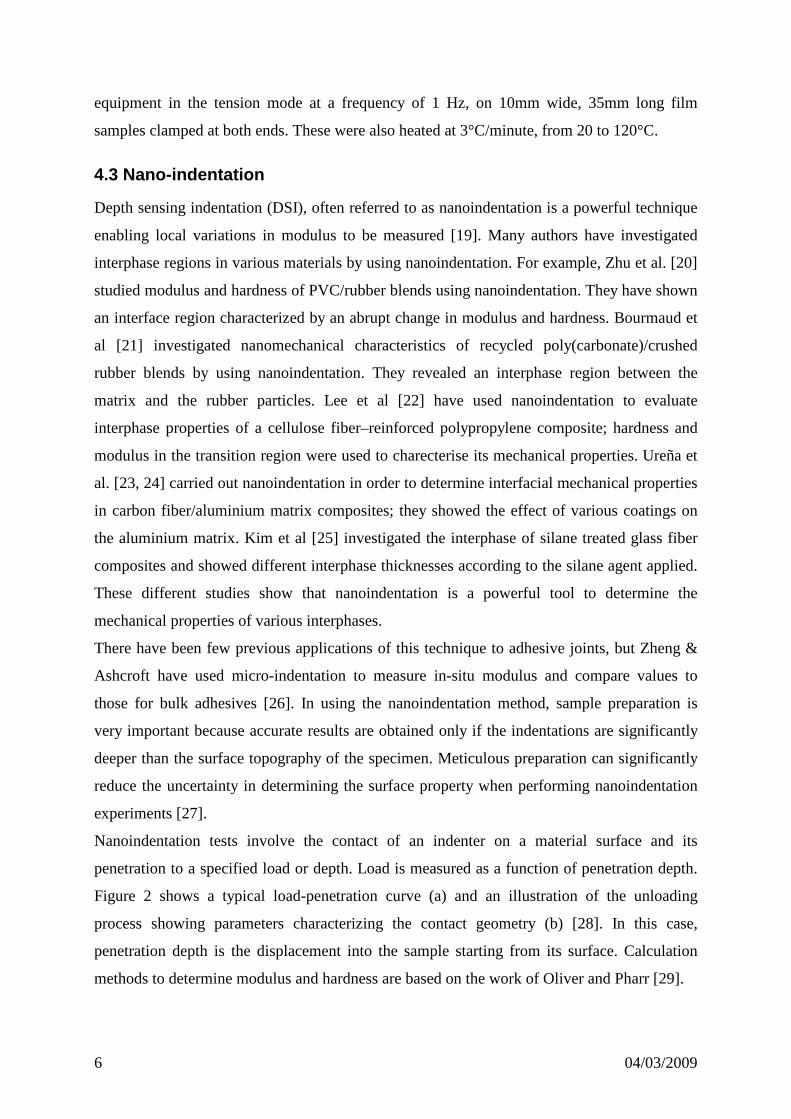
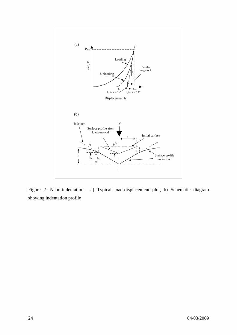
Nanoindentation tests involve the contact of an indenter on a material surface and its

penetration to a specified load or depth. Load is measured as a function of penetration depth.

Figure 2 shows a typical load-penetration curve (a) and an illustration of the unloading

process showing parameters characterizing the contact geometry (b) [28]. In this case,

penetration depth is the displacement into the sample starting from its surface. Calculation

methods to determine modulus and hardness are based on the work of Oliver and Pharr [29].

7 04/03/2009

From the load-penetration curve we can easily obtain the maximum displacement, hmax, the

maximum load on the sample, Pmax and the contact stiffness, S. S is the slope of the tangent

line to the unloading curve at the maximum loading point. The contact depth, hc is related to

the deformation behaviour of the material and the shape of the indenter. In fact hc = hmax – hs

as shown on Figure 2:

S

Phhc

maxmax ε−= (2)

where ε is a constant that depends on the geometry of the indenter (0.72 for a Berkovich

indenter). For a perfectly sharp Berkovitch indenter, projected area A can be calculated by Eq.

(3) as follows:

256.24 chA= (3)

The hardness is defined as the indentation load divided by the projected contact area, Eq. (4).

A

PH

max= (4)

The effective elastic modulus Er can be calculated with the relationship in Eq. (5):

AEaES rr πβ2

2 == (5)

where a is the contact radius and β is a constant depending on the geometry of the indenter

(1.034 for a Berkovitch tip). The reduced modulus, Er, accounting for deformation of both the

indenter and the sample, is given by:

( ) ( )i

i

r EEE

22 111 νν −+−= (6)

In the equation above, Ei (1140 GPa) and νi (0.07) are the elastic properties of the diamond

indenter. E and ν are the elastic modulus and Poisson’s ratio of the sample.

Indentation tests were performed with a commercial nanoindentation system (Nanoindenter

XP, MTS Nano Instruments) at room temperature (23 ± 1)°C with a continuous stiffness

measurement (CSM) technique. In this technique, an oscillating force at controlled frequency

and amplitude is superimposed onto a nominal applied force. The material, which is in contact

with the oscillating force, responds with a displacement amplitude and phase angle.

A three-sided pyramid (Berkovitch) diamond indenter was employed for the indentation tests.

The area function, which is used to calculate contact area Ac from contact depth hc, was

carefully calibrated by using a standard sample, prior to the experiments.

8 04/03/2009

The nanoindentation system is coupled with an optical microscope in order to control the

surface of the sample in situ. The precise coordinates of the position of the indent are

determined simultaneously to the observation of the surface.

Strain rate during loading was maintained at 0.05 s-1 for all the samples. We operated with a 3

nm amplitude, 70 Hz oscillation using identical load rate conditions. The nanoindenter tests

were carried out in the following sequence: first, after the indenter made contact with the

surface, it was driven into the material at a constant strain rate, 0.05 s-1 to a depth of 100 nm;

secondly, the load was held at maximum value for 60 s; and finally, the indenter was

withdrawn from the surface with the same rate as during loading until 10% of the maximum

load was reached.

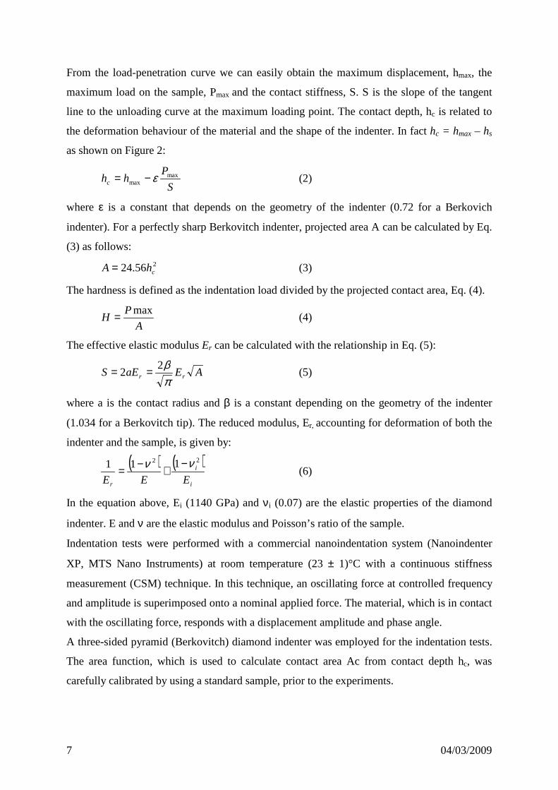
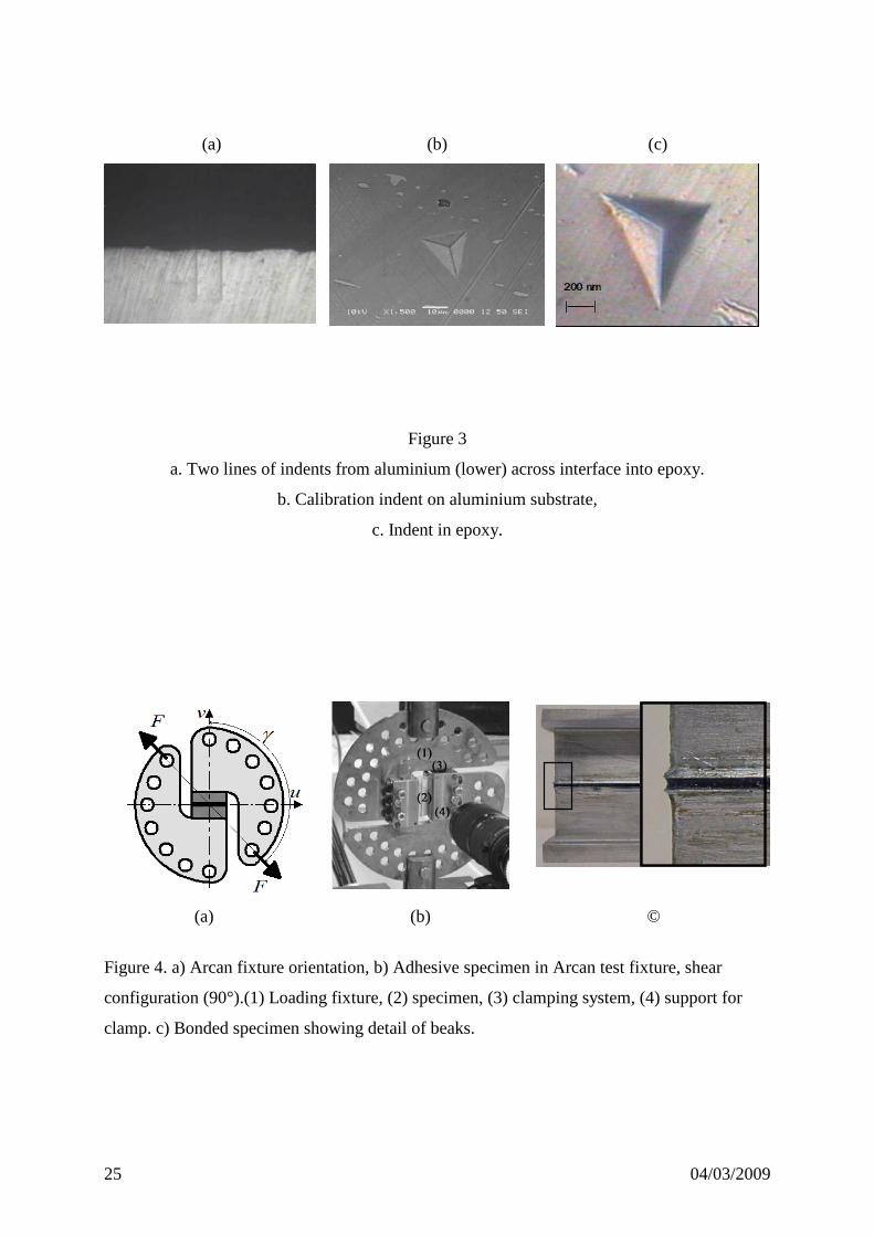
Figure 3a shows an example of two lines of 40 indents at the metal/epoxy interface. The

distance between two indents is 2 microns. It is easy to see the two lines of indents in the

aluminium, the lines continue into the epoxy above. Figure 3b shows an example of a single

indent in the aluminium, Figure 3c shows an indent in the epoxy. The surfaces were polished

using progressively finer paper then down to 0.5 microns diamond paste.

4.4 Spectroscopic analysis

There are various spectroscopic techniques which allow local measurements of molecular

structure to be made on polymers [30]. A Thermo Nicolet Infrared microscope was used first,

to try to obtain local spectra in reflection, but the reflected signal was too weak to allow

reliable analysis due to the high infrared absorption coefficients of epoxy samples.

Measurements might be possible in transmission but this would require very careful

preparation of thin sections. However, this equipment can only make measurements with a

spot greater than 100 µm², due to unfavourable spatial resolution of the microscope in the

infrared spectral domain. A solution is to carry out vibrational spectroscopy on epoxy samples

using Raman scattering spectroscopy; this provides similar information on sample features but

it allows measurements even if substrates strongly absorb infrared radiation. Using a visible

laser, high spatial resolution can be obtained. Raman scattering spectra were collected on a

Jobin-Yvon LabRam HR800 spectrometer equipped with an Olympus BX41 optical

microscope, an adjustable angle notch filter and an air cooled Andor iDus CCD camera. The

excitation was induced by a laser beam of a Sacher Lion Diode at a wavelength of 784.4 nm.

This equipment is in a controlled environment laboratory at 20°C ±1°C. The beam was

focused using a 100 x objective lens (numerical aperture = 0.90) on an area of about 3 µm².

The laser power on the sample was approximately 20 mW. The back-scattered Raman spectra

9 04/03/2009

were collected in a confocal mode to avoid optical artefacts. With a 600 l/mm grating, the

spectral resolution at 838 nm was 2.5 cm-1, with a wavenumber precision better than 1 cm-1.

The wave-number calibration is obtained by recording the band for silicon, located at 521

cm-1. The microscope is equipped with a x,y,z motorized stage which allows mapping

acquisition in autofocus mode. 21 spectra were recorded each 2.5 µm along a cross section of

50 µm on a thin (0.1 mm thickness) assembly sample. In this paper results from only 13

spectra are presented for clarity (see below).

4.5 Mechanical tests

The adhesive alone, in the form of parallel and dog-bone specimens cut from cast films of

different thicknesses, was first tested in tension on an Instron 4302 test frame with a 500 N

load cell. Loading rate was 2 mm/minute. Extension was measured on some parallel sided

10mm wide specimens using a clip-on Instron 2620-602 extensometer with 25mm gauge

length, but for the thinnest films (<0.5mm) the weight of the extensometer tended to deform

the specimen, so results were not reliable and are not presented. Tensile strength was

measured on dog-bone samples, with a central width of 10 mm and polished edges. Then

bonded aluminium joints were tested, in a modified Arcan fixture. This has been described in

detail previously [18,31]. Figure 4 shows the fixture. By changing the angle of the fixture

with respect to the machine loading axis loads from pure shear to pure tension can be applied.

Three types of loading were applied here, tension (loading with the fixture at 0° to the

machine axis), shear (loading with the fixture at 90° as shown in Figure 4) and a balanced

combination of tension and shear, by orienting the specimen at 45° to the loading axis.

Loading rate was 0.5 mm/minute for all samples. This will result in a slightly lower strain rate

for thicker bondline thicknesses, but results from previous studies suggest that this difference

will not change the response significantly [32].

The beaks, Figure 4c, enable a more uniform stress state to be achieved, but a correction is

applied to account for the small stress concentrations revealed by numerical analysis [18].

From the measured load and analysis of images of the displacements of the substrates during

the tests the mean stress can be plotted versus displacement (tangential DT or normal DN)

divided by joint thickness h. The direct study of displacements and strains within the bonded

joint is difficult due to the presence of the beaks and because the surface is not perfectly flat at

the edges of the specimen. As the adhesive thickness is small the displacements of the

substrates are used to determine strain in the joint. However, this measurement requires

validation if homogeneous strain through the joint thickness is to be assumed. In order to

10 04/03/2009

check this by analysing the displacements through the thickness of the bonded joint a special

specimen was prepared, with a 1.1mm thick adhesive bond-line and with the beak removed in

one zone studied with the camera; thus, by analysing a small zone it is possible to determine

the kinematics of the bonded joint deformation. The digital camera system employed has been

described previously [31]. For this test the sample was tested in pure shear, the crosshead

displacement rate of the tensile testing machine was 0.5 mm/min and an image was recorded

every second. On the images the thickness of the bonded joint (1.1mm) is represented with

nearly 550 pixels. The zone studied is a rectangle of 600 pixels x 230 pixels, which allows the

analysis of the displacement of 400 x 100 points in the adhesive. Figure 5 presents the

geometry of the zone studied, and a representation of the measured displacement field in the

adhesive joint at time t=60s. The displacement field appears to have a linear evolution with

respect to the x-axis (horizontal axis); at this time the relative displacement of the two ends of

the adhesive joint is DT = 0.042mm (during loading, displacements of both substrates are

observed). Then, after obtaining the displacement fields in the zones studied by image

correlation at each time, an optimisation technique is used to obtain a representation of the

displacement field of the adhesive. The vertical component of the displacement field in the

adhesive (VRi) is required at a given time, at each point Mi (Xi, Yi), in the following form:

VRi = a + b Xi (7)

where a and b are constants. The two unknowns { a,b } are obtained by the minimization of

the difference between the modelled values of displacement and the values measured for the

points Mi: (UMi, VMi); UMi and VMi are the horizontal and vertical components of the

displacement. Here only the vertical component of the displacement is used in order to

analyse the adhesive deformation, the horizontal component of the displacement is much

smaller than the vertical one. The values of measured displacements are known for N pixels

of the zone of study. By solving the following problem:

Minimization of Σ(i=1,N) { (V Ri - VMi)2} (8)

the unknowns are the solutions of a linear problem with two equations for each time:

N Σ(X i)

Σ(X i) Σ(X i)2

a

b =

Σ(V i)

Σ(X i Vi) (9)

In fact, for each image we obtain a representation of the displacement in the thickness of

the adhesive. In order to evaluate this representation the following error indicator is defined:

ζ = 1N{ Σ(i=1,N) { (a + b Xi - VMi)

2}} 0.5 (10)

11 04/03/2009

ζ represents the average distance between the modelled values of displacement and those

measured.

As the texture of the adhesive changes during loading and as the displacements are quite

large, the image analysis is performed in several steps, in order to obtain better results; thus to

take into account the complete displacement history, an upper bound of the error indicator (η)

is proposed. Figure 6-a shows the time evolution of the error indicators; the values are in mm

and have to be compared to the relative displacement of the two ends of the adhesive joint,

DT, at each time (figure 6-b). The minimal value of detectable displacement by image

correlation using multi-scale resolution techniques is less than 0.05 pixel, for images coded in

8 bits. Therefore, for the scale factor used, which corresponds to nearly 500 pixels per mm,

the order of magnitude of minimal measurable displacement is lower than 1 x 10-4 mm. The

previous analysis is therefore quite accurate and errors are very small (Figure 5).

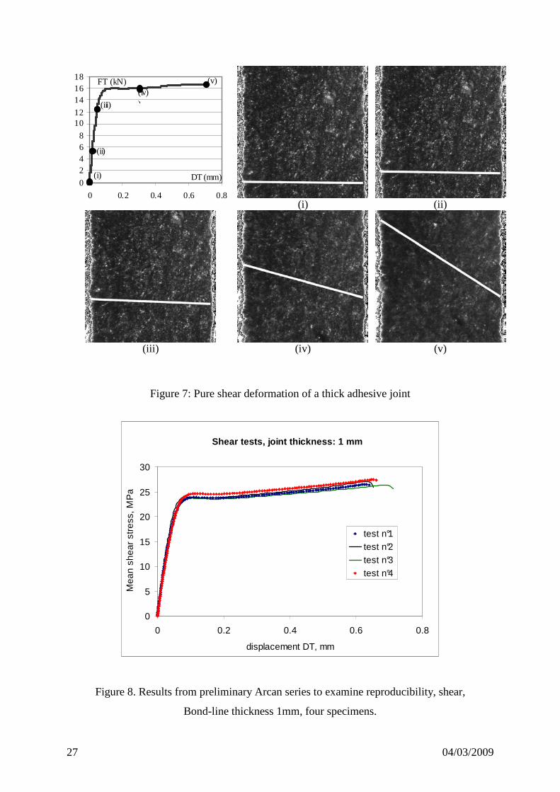
Figure 7 summarizes the results from this study; for different points on the loading curve it

shows the deformation across the adhesive joint and a linear regression representation of the

displacements in the thickness of the joint (thick white line). The assumption of homogeneous

deformation in the adhesive appears justified in the case of shear loading. The behaviour of

the adhesive close to the interface adhesive-substrate seems to be similar to that in the centre

of the joint, but a precise analysis of this zone is quite difficult as the surface of the substrate

is not perfectly flat. In order to establish the reproducibility of the method shear tests were

then performed on four nominally identical specimens prepared at the same time under

identical conditions. Figure 8 shows the results, and it is apparent that the response is quite

reproducible.

5. Results and discussion

5.1 Microscopic examination

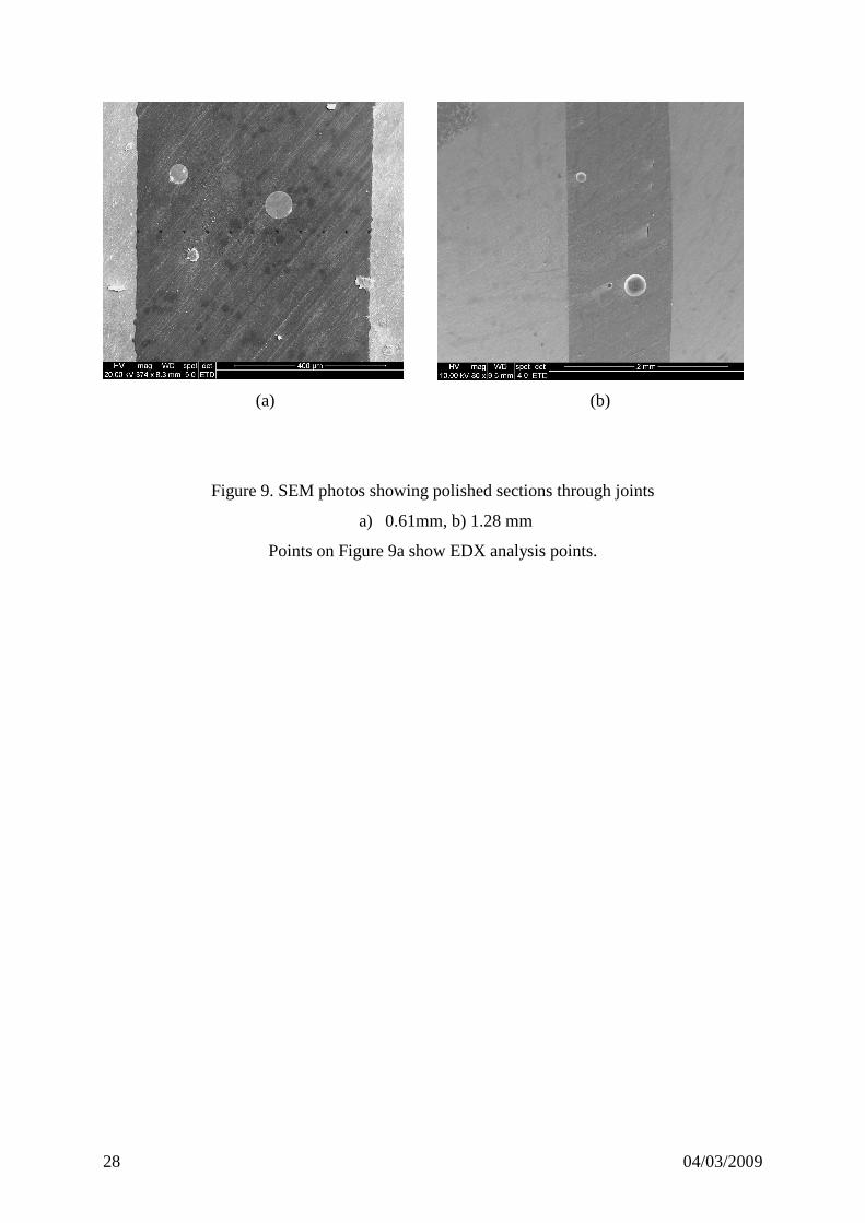
Figure 9 shows SEM photos of sections through joints of two thicknesses. While some

small defects are visible there is not a significant difference in terms of size or number of

defects between the two sections, and no significant difference was noted in other sections

examined. The spherical inclusions noted above are clearly visible. EDX analysis was

performed, the points across the joint in Figure 9a show the positions of one line of

measurements. These indicated no significant change in composition, but EDX sensitivity to

12 04/03/2009

the light elements C, O and N is limited. Analysis of the spheres clearly identified these to be

mainly silicon.

5.2 Thermal analysis

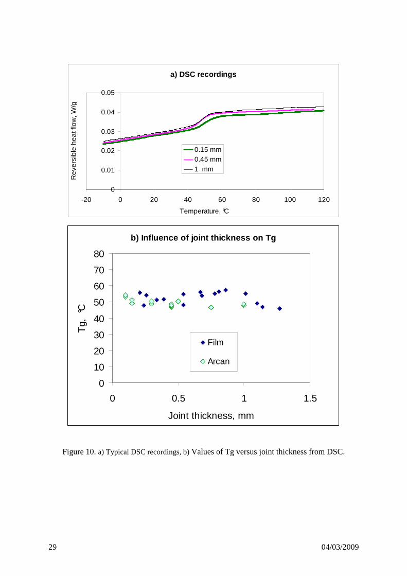
Figure 10a shows examples of the reversible part of DSC recordings for two samples of

different thickness. The values of glass transition temperature, Tg, defined as the point of

inflexion on the reversible enthalpy versus temperature plot, are shown in Figure 10b for

samples taken from joint fracture surfaces and from cast film samples. There is little

significant variation, all values are in the range 47 to 54°C, even though slightly higher values

are noted for the thinnest bond lines. If the substrate has modified the adhesive stoichiometry

over a significant difference (tens of microns) as was shown in previous studies by Roche [15]

when a higher hardener concentration was detected close to the substrate, one would expect

this to be revealed as a higher value of Tg for the thinnest joint. This is not the case here. The

values for the adhesive joints appear very similar to those obtained on thin and thick bulk film

specimens. When the temperature exceeds the Tg a small irreversible exothermic peak was

noted on the DSC plot. This indicates that cross-linking is not complete, and a higher

temperature cure would allow a higher Tg to be obtained, as has been discussed elsewhere

[18,33]. DMA also allowed Tg values to be obtained. According to the definition used

(change in slope of E’, peak tangent δ) these differ slightly from DSC values, but DMA

studies again indicated no difference in the small strain visco-elastic behaviour at different

thicknesses. Overall these thermal analysis results do not indicate any change in global

properties for different thicknesses of film or bond-line.

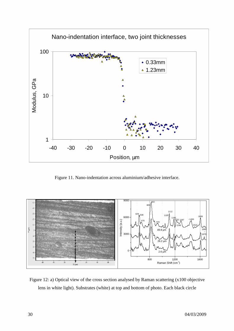
5.3 Nano-indentation

Nano-indentation was used to examine two aspects of the joints; first, to check the modulus of

joints in-situ, by indenting at mid-thickness, and second to examine the substrate/adhesive

interface region in order to determine whether an interphase was present. The results from the

check on modulus are presented in Table 1. These show very similar modulus values at the

centre of each joint, with a slight tendency towards higher values as thickness increases.

Joint thickness, mm Modulus, GPa

0.33

0.65

1.23

2.45 (0.11)

2.63 (0.19)

2.71 (0.15)

Table 1. Measured modulus values, mean ( standard deviation)

13 04/03/2009

of 10 values for each sample, measured at mid-thickness by nano-indentation.

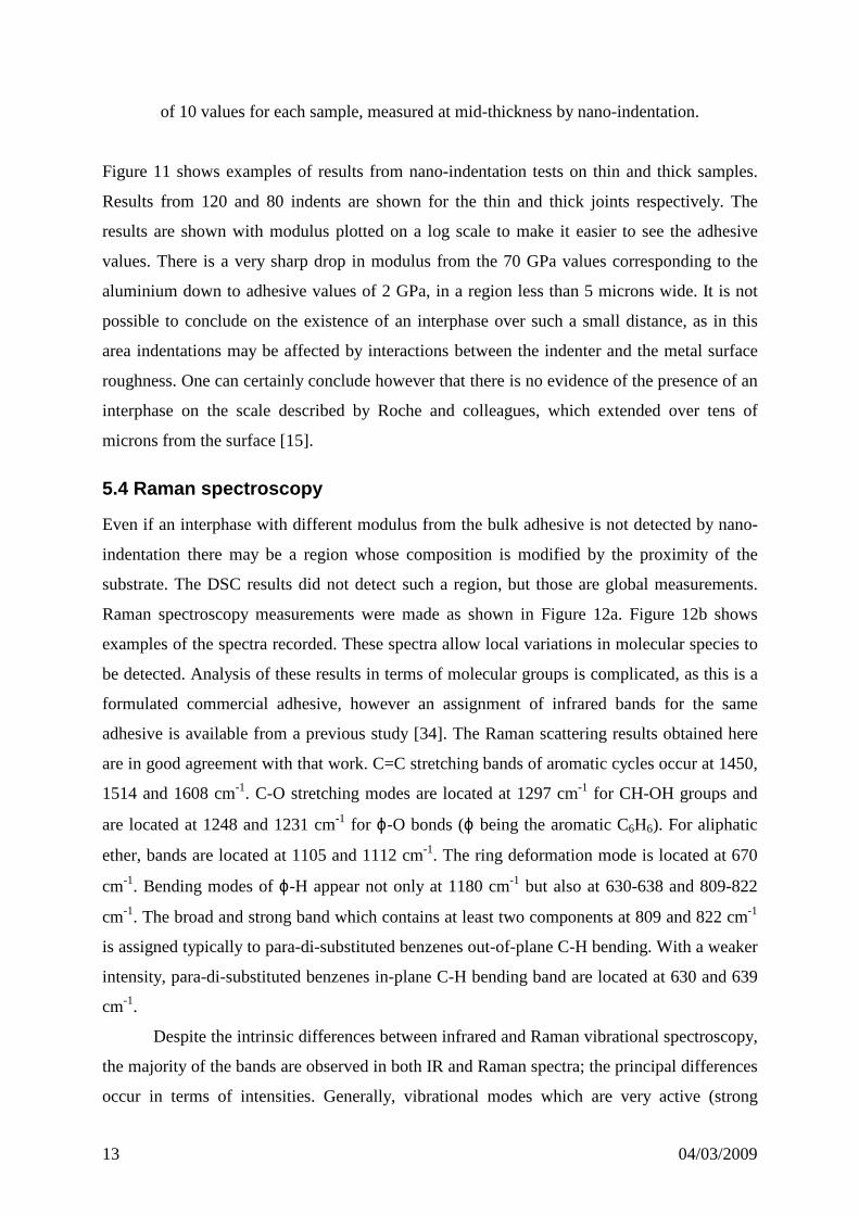
Figure 11 shows examples of results from nano-indentation tests on thin and thick samples.

Results from 120 and 80 indents are shown for the thin and thick joints respectively. The

results are shown with modulus plotted on a log scale to make it easier to see the adhesive

values. There is a very sharp drop in modulus from the 70 GPa values corresponding to the

aluminium down to adhesive values of 2 GPa, in a region less than 5 microns wide. It is not

possible to conclude on the existence of an interphase over such a small distance, as in this

area indentations may be affected by interactions between the indenter and the metal surface

roughness. One can certainly conclude however that there is no evidence of the presence of an

interphase on the scale described by Roche and colleagues, which extended over tens of

microns from the surface [15].

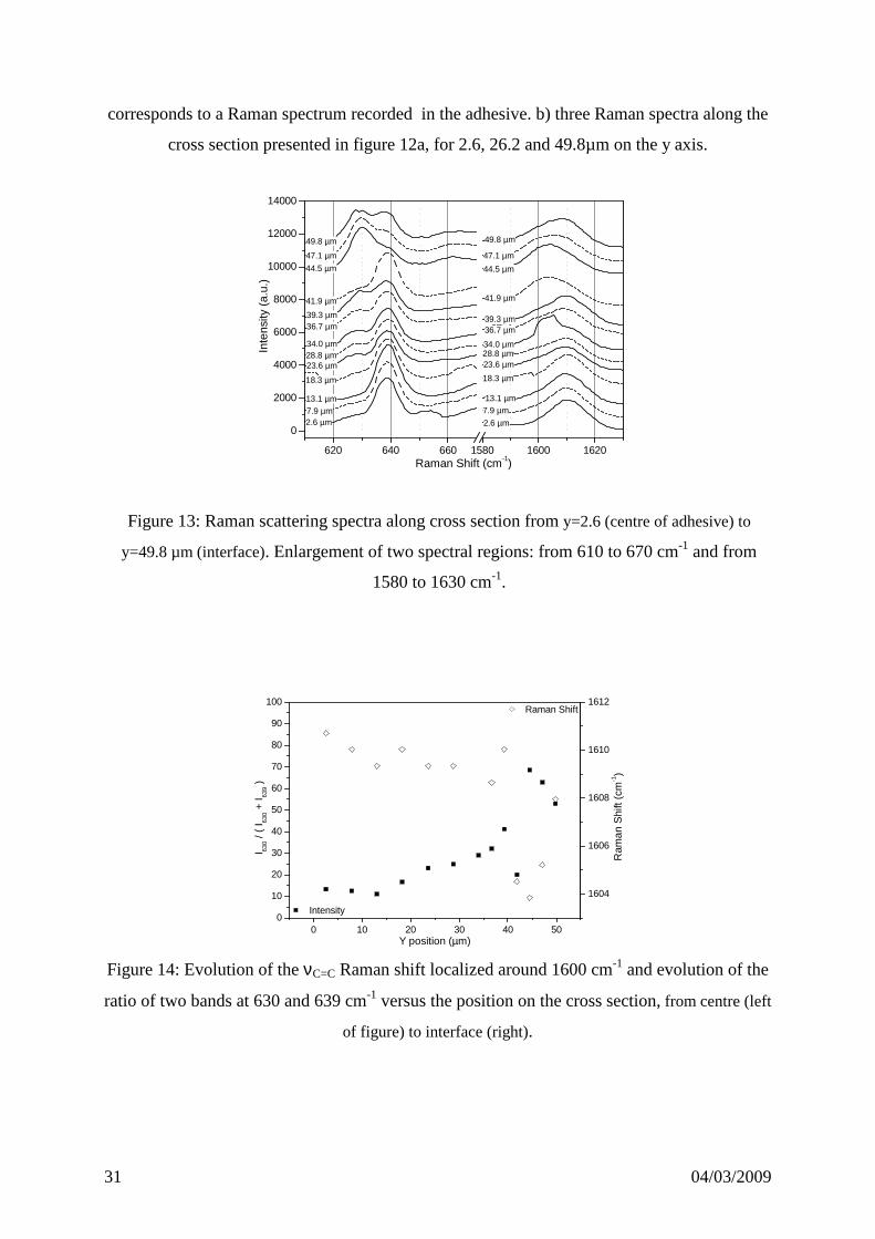
5.4 Raman spectroscopy

Even if an interphase with different modulus from the bulk adhesive is not detected by nano-

indentation there may be a region whose composition is modified by the proximity of the

substrate. The DSC results did not detect such a region, but those are global measurements.

Raman spectroscopy measurements were made as shown in Figure 12a. Figure 12b shows

examples of the spectra recorded. These spectra allow local variations in molecular species to

be detected. Analysis of these results in terms of molecular groups is complicated, as this is a

formulated commercial adhesive, however an assignment of infrared bands for the same

adhesive is available from a previous study [34]. The Raman scattering results obtained here

are in good agreement with that work. C=C stretching bands of aromatic cycles occur at 1450,

1514 and 1608 cm-1. C-O stretching modes are located at 1297 cm-1 for CH-OH groups and

are located at 1248 and 1231 cm-1 for ϕ-O bonds (ϕ being the aromatic C6H6). For aliphatic

ether, bands are located at 1105 and 1112 cm-1. The ring deformation mode is located at 670

cm-1. Bending modes of ϕ-H appear not only at 1180 cm-1 but also at 630-638 and 809-822

cm-1. The broad and strong band which contains at least two components at 809 and 822 cm-1

is assigned typically to para-di-substituted benzenes out-of-plane C-H bending. With a weaker

intensity, para-di-substituted benzenes in-plane C-H bending band are located at 630 and 639

cm-1.

Despite the intrinsic differences between infrared and Raman vibrational spectroscopy,

the majority of the bands are observed in both IR and Raman spectra; the principal differences

occur in terms of intensities. Generally, vibrational modes which are very active (strong

14 04/03/2009

bands) in infrared are inactive (weak bands) in Raman scattering and conversely. Thus, one of

the advantages of Raman scattering spectroscopy is that the C=C group has a strong stretching

vibration band which is generally weak or inactive in infrared. This band can often be used to

determine polymer conformations and to determine the extent of cross-linking [35]. As a

consequence, ϕ-H bending modes could be useful to observe the chemical vicinity of

aromatic cycles so the C-H bending bands and C=C stretching bands behaviour has been

examined along the joint cross section. These bands are plotted in figure 13 in two spectral

regions from 610 to 670 cm-1 for C-H bending and from 1580 to 1630 cm-1 for C=C

stretching.

The first spectral region exhibits a decrease of the 639 cm-1 bands to the benefit of the 630

one. As for the second spectral region, the C=C stretching band located at 1604 cm-1 at the

y=2.6 µm position shifts to higher values around 1609 cm-1 and there are changes in width and

shape. In order to study these variations through the cross section, figure 14 is obtained by

plotting intensity ratio (left axis) and Raman shift (right axis) for each analysed point of the

cross section.

The ratio is obtained by dividing the intensity of the band located at 630 cm-1 by the

addition of the intensities of the bands located at 630 and 639 cm-1. The results are presented

as a percentage. Variations are clearly present for both parameters ; the last 10 µm before

reaching the substrate show the largest variations. These results suggest that in the adhesive

close to the interface the chemical behaviour of the aromatic cycle in the resin changes. Two

hypotheses could be proposed: either the observed variations are due to stoichiometric ratio

variation of hardener and polymer and/or they are due to different resin conformations

between bulk and interface adhesive.

The results shown here are from a preliminary study to determine whether Raman

spectroscopy can be useful in analysing adhesive joints. To interpret the results in more detail

is beyond the scope of the present work, but it is clear that Raman spectroscopy provides a

very sensitive tool to examine local variations in composition, and that for the joint studied

here chemical changes appear to be localized to a very small region near the substrate, within

10µm.

5.5 Mechanical tests

Mechanical tests were then performed, first on films then on bonded joints. Figure 15 shows

examples of the first part of tensile stress-strain curves measured on parallel sided samples to

determine modulus values for thin (mean 0.64mm) and thick (mean 1.25mm) specimens.

15 04/03/2009

Failures often occurred prematurely at the extensometer knife edges but tensile modulus

values could be determined from initial slopes. These are very similar for both thickness

ranges. The values are lower than those obtained by nanoindentation (Table 1), as is usually

observed due to various factors including the higher loading rate for the latter, the stress state

beneath the indenter and surface effects. Figure 16 shows tensile strengths from tests on dog-

bone specimens without the extensometer.

Results from these tests do not indicate an influence of thickness on tensile properties of cast

films, suggesting that there is no intrinsic reason to expect an influence of thickness on

adhesive joint behaviour. Jeandrau has shown that a reasonable estimation of joint properties

may be obtained from bulk adhesive behaviour in some cases [36]. These tests also allowed

values of E and σy to be determined, which can be introduced in the equation proposed by

Kinloch & Shaw (equation 1). A value of Gc is also needed if rp is to be calculated, and this

was measured during a previous study using tapered double cantilever beam (TDCB)

specimens [37] to be around 1400 J/m². The calculated plastic zone size rp is then around

0.3mm, so the optimal joint thickness with respect to fracture energy is around 0.6mm.

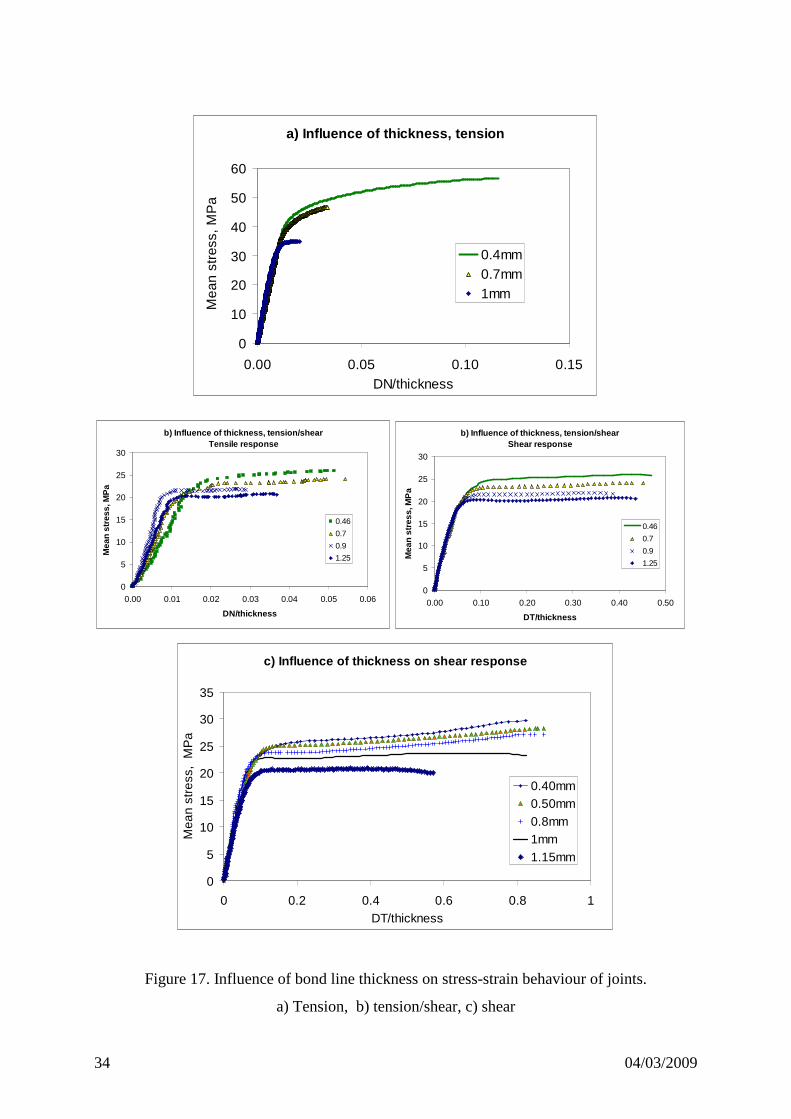
Adhesively bonded joints were then tested in the modified Arcan fixture. Figure 17

shows examples of results from 12 specimens, indicating how bond line thickness affects the

stress-strain response under tension, tension/shear and shear loading using the Arcan fixture.

Mean stress is plotted versus displacement/thickness, as in order to determine the material

behaviour law an inverse identification procedure is required [32].

There is an influence of bond-line thickness under shear and tension/shear loads on the

plateau values, with a much larger influence for tensile loading. In all the cases examined here

lower plateau values were obtained for thicker joints. The failure mode was cohesive for

tensile loading but adhesive for shear and tension/shear loads. Failure stresses are higher in

tension than in shear, but failure strains are much larger in shear. Figure 18 shows the

deformation of a joint during pure shear loading before failure, the shear bands are clearly

visible. It is interesting to note that the tensile strengths obtained on film samples are similar

to the mean tensile stress at failure of the thickest joints, whereas considerably higher

strengths were obtained on adhesive samples with thin bond-lines. The constraint on lateral

movement imposed by the substrates has a strong effect on thin film behaviour, the Poisson

effect in thicker films is more similar to that of bulk tensile specimens. Modulus values from

bulk film tests are not compared with Arcan tensile results due to uncertainty in the very small

strains measured in the latter.

16 04/03/2009

5.6 Numerical analysis of the influence of joint thickness

In order to understand the influence of bond line thickness noted in the previous section

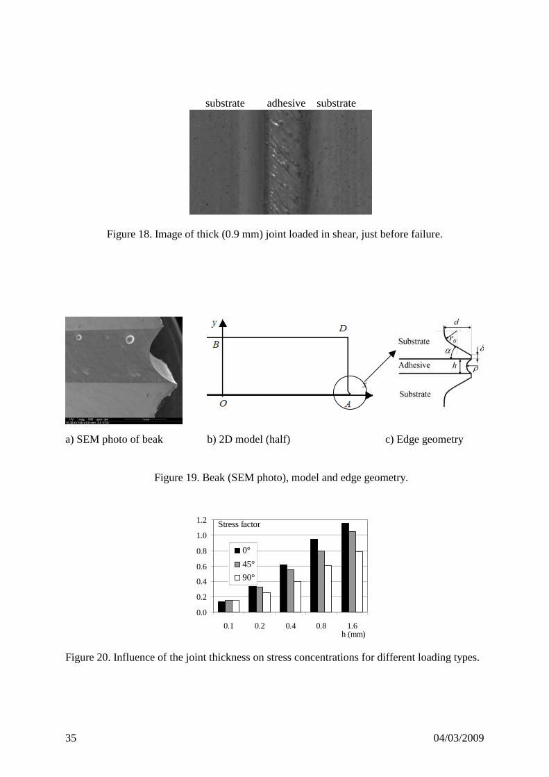
numerical modelling of the test geometry was performed, using CAST3M finite element

software [38]. Figure 19a shows an SEM image of a polished section in the beak region and

Figures 19 b and c show the model geometry.

A study of the stress distribution through the thickness of the adhesive joint, even

assuming linear elastic behaviour of the components, requires refined meshes [39]. Various

simulations have shown that good numerical results are obtained using meshes with at least

20 linear rectangular elements for a 0.1mm thickness of adhesive [40]. The geometry of the

specimens designed for the modified Arcan fixture is presented in Figure 18b (BD=33mm,

OB=15mm). The model boundary conditions are anti-symmetric on the segment OA, in order

to model only half of the structure and displacements are applied to the upper bound of the

substrate BD (in the y-direction for tensile loading and in the x-direction for shear loading).

Results are presented for aluminium substrates (Young’s modulus: Ea=80 GPa, Poisson's

ratio: νa=0.3); the material parameters for the adhesive joint are Ej=2 GPa, νj=0.3.

Calculations were made in 2D (plane stress) for different thicknesses of the adhesive joint (h)

under tensile loading (0°), tensile-shear loading (45°) and shear loading (90°) using the

following parameters: h=0.1mm, d=0.5mm, r0=0.8mm and α=45° (see Figure 19c).

The equivalent von Mises stress is used to compare stress states and results are normalised

to make analysis of the stress distributions easier; the von Mises equivalent stress is

normalized to unity at the middle of the joint (point O, Figure 19b).

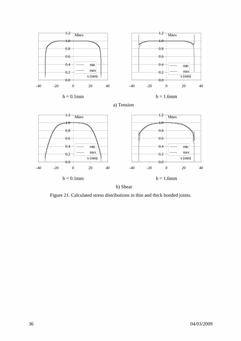
Figure 20 presents the value of the von Mises equivalent stress near the free edge of the

joint (stress factor), normalized with respect to the value at the centre of the joint. An increase

in the thickness of the adhesive joint increases the edge effects. It is important to note that the

loading conditions have an influence on the edge effects, and these are larger for tensile

loading than for shear. The influence of other parameters can be found in [41], for instance

edge effects are larger for steel substrates than for aluminium ones with this experimental

fixture. Figure 21 presents the maximum and minimum values of the von Mises equivalent

stress in the thickness of the adhesive joint along the bond line (direction x in Figure 19b).

Two extreme cases are considered, joint thicknesses (h) of 0.1 and 1.6mm. These results show

that not only the maximum stress (stress factor presented above, Figure 20) but also the stress

distributions in the adhesive joint depend on the thickness of the adhesive joint. Moreover it is

17 04/03/2009

important to note that the stress gradients close to the free edges of the adhesive increase

significantly with the joint thickness.

The results in Figures 20 and 21 clearly show that in order to obtain a valid

characterization of adhesive joint behaviour using this test fixture it is necessary to limit the

bond-line thickness. While it is hazardous to use numerical results to make quantitative

statements the trends from tests and analyses suggest that for shear loading with this test

fixture joints up to 0.8 mm may be used, while in tension it is preferable to keep the bond line

thickness below 0.6mm.

Conclusions

This study has examined the physico-chemical and mechanical behaviour of aluminium

substrates bonded with epoxy adhesive joints of different thicknesses. There is no evidence

that changing the joint thickness results in significant modifications to the polymer structure,

the interface region nor the presence of defects for this assembly, over the range from 0.2 to

1.3 mm. More sophisticated analyses would be needed to reveal local changes in chemistry

but variations detected by Raman spectroscopy and nano-indentation were confined to a very

thin layer near the substrate, whose extent is similar to the substrate surface roughness. The

tensile stiffness and strength of cast adhesive films showed no variation over the same range

of thickness. For adhesively bonded aluminium assemblies tested using the modified Arcan

fixture a small influence of bond line thickness was noted under shear and tension/shear

loads; a small reduction in mechanical properties was noted as bond line thickness was

increased. Under tensile loading a more pronounced effect was measured, with significantly

lower yield stress and failure strain for thicker joints. Numerical analysis indicates that this is

caused by a change in the stress state as thicker joints are tested. The stress concentrations are

higher for tension loading than tension/shear and lowest in shear, and all increase with

thickness. It is recommended that for this modified Arcan test bond line thickness be limited

to 0.6 mm to characterize these joints in tension with this fixture, and to below 0.8 mm for

tension/shear and pure shear. The thinner the joint the lower the edge effects and the lower the

influence of test imperfections such as misalignment. Further work is focussing on the

characterization of the effects of marine aging on the performance of these joints.

18 04/03/2009

Acknowledgements

The authors are grateful to Philippe Crassous (IFREMER), for help with the SEM

observations.

References

[1] Adams RD (editor), Adhesive Bonding, Science, Technology and Applications, Woodhead

Publishing, 2005.

[2] Kinloch AJ, Adhesion and Adhesives, Science and Technology, Chapman and Hall, 1987.

[3] Adams RD, Peppiatt NA, Stress Analysis of Adhesive-Bonded Lap Joints J. Strain Analysis, 1974,

9, 185-196.

[4] Bascom WD, Cottington RL, Timmons CO, Fracture reliability of structural adhesives, J. Appl

Polymer Sci., Applied Polymer Symp., 32, 1977, 165-188.

[5] Kinloch AJ, Shaw SJ, The fracture resistance of a toughened epoxy adhesive, J. Adhesion, 1981,

12, 59-77.

[6] Kinloch AJ, Moore DR, The influence of adhesive bond line thickness on the toughness of

adhesive joints, in The application of fracture mechanics to polymers, adhesives and composites, ed

Moore DR, Elsevier 2004, 149-155.

[7] Kawashita LF, Kinloch AJ, Moore DR, Williams JG, The influence of bond line thickness and peel

arm thickness on adhesive fracture toughness of rubber toughened epoxy-aluminium alloy laminates,

Int Jadhesion & Adhesives, 28, 2008, 199-210.

[8 ] Mall S, Ramamurthy G, Effect of bond thickness on fracture and fatigue strength of adhesively

bonded composite joints, Int J. Adhesion & Adhesives, 9, 1, 1989, 33-37.

[9] Gleich DM; Van Tooren MJL; Beukers A, A stress singularity approach to failure initiation in a

bonded joint with varying bondline thickness, J. Adhes. Sci & Tech., 15, 10, 2001, 1247-1259. [9]

[10] Tamblin JS, Yang C, Harter P, Investigation of thick bond line adhesive joints, DOT/FAA/AR-

01/33, June 2001.

[11] Grant LDR, Adams RD, DaSilva LFM, Experimental and numerical analysis of single lap joints

for the automotive industry, Int J. Adhesion & Adhesives, 29, 2009, 405-413.

[12] Taib AA, Boukhili R, Achiou S, Gordon S, Boukehili H, Bonded joints with composite

adherends. Part 1. Effect of specimen configuration, adhesive thickness, spew fillet and adherend

stiffness on fracture, Int J. Adhesion & Adhesives, 26, 2006, 226-236.

[13] Jarry E, Shenoi RA, Performance of butt strap joints for marine applications, Int J Adhesion and

Adhesives 26, 2006, 162-176.

[14] Nairn JA, Energy release rate analysis for adhesive and laminate double cantilever beam

specimens emphasizing the effect of residual stresses, Int. J Adhesion & Adhesives, 20, (2000), 59-70.

19 04/03/2009

[15] Roche AA, Bouchet J, Bentadjine S, Formation of epoxy-diamine interphases, Int J Adhesion and

Adhesives, 22, 2002, 431-441.

[16] Jansen I, Schneider D, Hassler R, Laser-acoustic, thermal and mechanical methods for

investigations of bond lines, Int J. Adhesion & Adhesives, 29, 2009, 210-216.

[17] Possart G, Presser M, Passlack S, Geiss PL, Kopnarski M, Brodyanski A, Steinmann P, Micro-

macro characterisation of DGEBA-based epoxies as a preliminary to polymer interphase modelling,

Int J. Adhesion & Adhesives (2008), doi:10.1016/j.ijadhadh.2008.10.001

[18] Cognard J.Y., Davies P., Sohier L., Créac’hcadec R., A study of the non-linear behaviour of

adhesively-bonded composite assemblies, Composite Structures, Vol. 76, 2006, 34-46.

[19] Fischer-Cripps C., Nanoindentation, Springer 2002.

[20] Shui-Han Zhu, C.-M.C., Yiu-Wing Mai,, Micromechanical properties on the surface of PVC/SBR

blends spatially resolved by a nanoindentation technique. Polymer Engineering and Science, 2004.

44(3): p. 609-614.

[21] Bourmaud, A., et al., Investigation of the polycarbonate/crushed-rubber-particle interphase by

nanoindentation. Journal of Applied Polymer Science, 2007. 103(4): p. 2687-2694.

[22] Lee, S.-H., et al., Evaluation of interphase properties in a cellulose fiber-reinforced polypropylene

composite by nanoindentation and finite element analysis. Composites Part A: Applied Science and

Manufacturing, 2007. 38(6): p. 1517-1524.

[23] Campo, M., A. Ureña, and J. Rams, Effect of silica coatings on interfacial mechanical properties

in aluminium--SiC composites characterized by nanoindentation. Scripta Materialia, 2005. 52(10): p.

977-982.

[24] Ureña, A., et al., Characterization of interfacial mechanical properties in carbon fiber/alhuminium

matrix composites by the nanoindentation technique. Composites Science and Technology, 2005.

65(13): p. 2025-2038.

[25] Kim, J.-K., M.-L. Sham, and J. Wu, Nanoscale characterisation of interphase in silane treated

glass fibre composites. Composites Part A: Applied Science and Manufacturing, 2001. 32(5): p. 607-

618.

[26] Zheng S, Ashcroft IA, A depth sensing indentation study of the hardness and modulus of

adhesives, Int J Adhesion & Adhesives, 25, 2005, 67-76.

[27] L. Shen, T. Liu, P. Lv. Polishing effect on nanoindentation behavior of nylon 66 and its

nanocomposites. Polymer Testing 2005;24(6):746.

[28] X. Li, B. Bhushan. A review of nanoindentation continuous stiffness measurement technique and

its applications. Materials Characterization 2002;48(1):11.

[29] Oliver WC, Pharr GM, An improved technique for determining hardness and elastic-modulus

using load and displacement sensing indentation experiments, J Mater Res, 1992, 7, 1564-1583.

[30] Koenig JL, Spectroscopy of polymers, 2nd edition, Elsevier 1999.

20 04/03/2009

[31] Cognard JY, Davies P, Gineste B, Sohier L, Development of an improved adhesive test method

for composite assembly design, Composites Science & Technology - March 2005; 65 (3-4) 359-368.

[32] Créach’cadec R, Cognard J-Y, Heuzé T, On modelling the non-linear behaviour of thin adhesive

films in bonded assemblies with interface elements, J. Adhesion Sci. & Tech., 2008, available on-line.

[33] Lapique F, Radford K, Curing effects on viscosity and mechanical properties of a commercial

epoxy resin adhesive, Int J Adhesion and Adhesives, Vol. 22, 4, 2002, 337-346

[34] Chaignaud S, Durability of elastomer/metal assemblies, PhD thesis Université de Toulon et du

Var, October 2003 (in French).

[35] Socrates G, Infrared and Raman Characteristic Group Frequencies, Tables and Charts, Wiley, 3rd

edition, 2001.

[36] Jeandrau JP, Analysis and design data for adhesively bonded joints, Int J Adhes & Adhesives, 11,

2, April 1991, 71-79.

[37] Ducept F, Davies P, Gamby D, Mixed mode failure criteria for a glass/epoxy composite and an

adhesively bonded composite/composite joint, Int J Adhesion & Adhesives, 20, 2000, 233-244.

[38] J.Y. Cognard, F. Thomas, P. Verpeaux, An integrated approach to solving mechanical problems

on parallel computers, Advances in Engineering Software, 31, 885-899, 2000.

[39] Cheikh M, Coorevits P, Loredo M., Modelling the stress vector continuity at the interface of

bonded joints, Int. J. Adhesion & Adhesives, 22, 249-257, 2001.

[40] Cognard J.Y., Créac’hcadec R., Davies P, Sohier L., Numerical modelling of the non-linear

behavior of adhesively-bonded assemblies, in Innovation In Engineering Computational Structures

Technology, Saxe-Coburg Publications, ISBN 1-874672-27-X, 225-247, 2006.

[41] Cognard J.Y., Numerical analysis of edge effects in adhesively-bonded assemblies. Application to

the determination of the adhesive behaviour, Computers & Structures, 2008 (accepted for publication).

21 04/03/2009

List of Figure headings.

Figure 1. a) Assembly fixture for 6 Arcan specimens in oven. b) Arcan samples with three thicknesses,

sections after high pressure water-jet cutting.

Figure 2. Nano-indentation. a) Typical load-displacement plot, b) Schematic diagram showing

indentation profile

Figure 3a. Two lines of indents from aluminium (lower) across interface into epoxy.

b. Calibration indent on aluminium substrate, c. Indent on epoxy.

Figure 4. a) Arcan fixture orientation, b) Adhesive specimen in Arcan test fixture, shear configuration

(90°).(1) Loading fixture, (2) specimen, (3) clamping system, (4) support for clamp. c) Bonded

specimen showing detail of beaks.

Figure 5: Zone studied and displacement field at t=60s, 1.1 mm thick bondline

Figure 6: time evolution of the error indicator and relative displacement

Figure 7: Pure shear deformation of a thick adhesive joint

Figure 8. Results from preliminary Arcan series to examine reproducibility, pure shear, bond line

thickness 1mm, four specimens.

Figure 9. SEM photos showing polished sections through joints

a) 0.61mm, b) 1.28 mm. Points on photo a) indicate EDX analysis points.

Figure 10. a) Typical DSC recordings, b) Values of Tg versus joint thickness from DSC.

Figure 11. Nano-indentation across aluminium/adhesive interface.

Figure 12: a) Optical view of the cross section analysed by Raman scattering (x100 objective lens in

white light). Substrates (white) at top and bottom of photo. Each black circle corresponds to a

Raman spectrum recorded, in the adhesive, b): three Raman spectra along the cross section presented

in figure 12a, for 2.6, 26.2 and 49.8µm on the y axis.

Figure 13: Raman scattering spectra along cross section from y=2.6 (centre of adhesive) to y=49.8 µm

(interface). Enlargement of two spectral regions: from 610 to 670 cm-1 and from 1580 to 1630 cm-1.

Figure 14: Evolution of the nC=C Raman shift localized around 1600 cm-1 and evolution of the ratio of

two bands at 630 and 639 cm-1 versus the analysed points along cross section, from centre (left of

figure) to interface (right).

Figure 15. Typical tensile stress-strain plots parallel-sided film specimens, and mean modulus values

with standard deviations (calculated over strain range 0.1-0.3%) for thin and thick specimens. Six

specimens were tested for each thickness range.

Figure 16. Strength results from tensile tests on films, dogbone specimens.

Figure 17. Influence of bond line thickness on stress-strain behaviour of joints.

a) Tension (0°), b) Tension/shear (45°), c) Shear (90°)

Figure 18. Image of thick (0.9 mm) joint loaded in shear, just before failure

Figure 19. Beak (SEM photo), model and edge geometry.

Figure 20. Influence of the thickness of the joint on stress concentrations for different loading types.

22 04/03/2009

Figure 21. Calculated stress distributions in thin and thick bonded joints, a)Tension, b) Shear.

23 04/03/2009

Specimen Specimen

(a) (b)

Figure 1. a) Assembly fixture for six Arcan specimens in oven.

b) sections through samples with three thicknesses

24 04/03/2009

Loa

d, P

Unloading

Displacement, h

Loading

S

Possible range for hc

hf hmax

Pmax

hc for ε = 1 hc for ε = 0.72

(a)

P Indenter

Initial surface

h hc

hf

hs

a

(b)

Surface profile after load removal

Surface profile under load

Figure 2. Nano-indentation. a) Typical load-displacement plot, b) Schematic diagram

showing indentation profile

25 04/03/2009

(a) (b) (c)

Figure 3

a. Two lines of indents from aluminium (lower) across interface into epoxy.

b. Calibration indent on aluminium substrate,

c. Indent in epoxy.

(a) (b) ©

Figure 4. a) Arcan fixture orientation, b) Adhesive specimen in Arcan test fixture, shear

configuration (90°).(1) Loading fixture, (2) specimen, (3) clamping system, (4) support for

clamp. c) Bonded specimen showing detail of beaks.

26 04/03/2009

� substrate adhesive substrate �

0 mm 0.042mm

Figure 5: Zone studied and displacement field at t=60s, 1.1mm thick bondline

Error indicator (mm)

0.000

0.002

0.004

0.006

0.008

0.010

0.012

0 50 100 150time (s)

ζη

DT (mm)

0

0.1

0.2

0.3

0.4

0.5

0.6

0.7

0.8

0 50 100 150

time (s)

(a) error indicator (b) relative displacement

Figure 6: time evolution of the error indicator and relative displacement

27 04/03/2009

Figure 7: Pure shear deformation of a thick adhesive joint

Shear tests, joint thickness: 1 mm

0

5

10

15

20

25

30

0 0.2 0.4 0.6 0.8

displacement DT, mm

Mea

n sh

ear

stre

ss, M

Pa

test n°1test n°2test n°3test n°4

Figure 8. Results from preliminary Arcan series to examine reproducibility, shear,

Bond-line thickness 1mm, four specimens.

FT (kN)

0

2468

1012

141618

0 0.2 0.4 0.6 0.8

DT (mm)(i)

(iii)

(iv))

(v)

(ii)

(i)

(ii)

(iii)

(iv)

(v)

28 04/03/2009

(a) (b)

Figure 9. SEM photos showing polished sections through joints

a) 0.61mm, b) 1.28 mm

Points on Figure 9a show EDX analysis points.

29 04/03/2009

a) DSC recordings

0

0.01

0.02

0.03

0.04

0.05

-20 0 20 40 60 80 100 120

Temperature, °C

Rev

ersi

ble

hea

t flo

w, W

/g

0.15 mm0.45 mm1 mm

b) Influence of joint thickness on Tg

0

10

20

30

40

50

60

70

80

0 0.5 1 1.5

Joint thickness, mm

Tg,

°C

Film

Arcan

Figure 10. a) Typical DSC recordings, b) Values of Tg versus joint thickness from DSC.

30 04/03/2009

Nano-indentation interface, two joint thicknesses

1

10

100

-40 -30 -20 -10 0 10 20 30 40

Position, µm

Mod

ulus

, GP

a

0.33mm1.23mm

Figure 11. Nano-indentation across aluminium/adhesive interface.

800 1200 1600

0

3000

6000

9000

1514

1660 ~1670

1608

~14501297

1248

12311180

1112

1105

915

822

809

670

638

49.8 µm

26.2 µm

Inte

nsity

(a.

u.)

Raman Shift (cm-1)

2.6 µm

629

Figure 12: a) Optical view of the cross section analysed by Raman scattering (x100 objective

lens in white light). Substrates (white) at top and bottom of photo. Each black circle

31 04/03/2009

corresponds to a Raman spectrum recorded in the adhesive. b) three Raman spectra along the

cross section presented in figure 12a, for 2.6, 26.2 and 49.8µm on the y axis.

620 640 660 1580 1600 1620

0

2000

4000

6000

8000

10000

12000

14000

49.8 µm49.8 µm

47.1 µm47.1 µm

44.5 µm44.5 µm

41.9 µm41.9 µm

39.3 µm39.3 µm

36.7 µm36.7 µm

34.0 µm34.0 µm28.8 µm28.8 µm23.6 µm23.6 µm

18.3 µm 18.3 µm

13.1 µm13.1 µm7.9 µm7.9 µm2.6 µm

Inte

nsity

(a.

u.)

Raman Shift (cm-1)

2.6 µm

Figure 13: Raman scattering spectra along cross section from y=2.6 (centre of adhesive) to

y=49.8 µm (interface). Enlargement of two spectral regions: from 610 to 670 cm-1 and from

1580 to 1630 cm-1.

0 10 20 30 40 500

10

20

30

40

50

60

70

80

90

100

1604

1606

1608

1610

1612

Intensity

I 630 /

( I 63

0 + I 63

9 )

Y position (µm)

Ram

an S

hift

(cm

-1)

Raman Shift

Figure 14: Evolution of the νC=C Raman shift localized around 1600 cm-1 and evolution of the

ratio of two bands at 630 and 639 cm-1 versus the position on the cross section, from centre (left

of figure) to interface (right).

32 04/03/2009

Tensile tests on films (parallel-sided specimens)

y(0.64mm) = 1802x + 0.3R² = 0.9999

y(1.19mm) = 1783x - 0.4R² = 0.9999

0

5

10

15

20

25

0 0.005 0.01 0.015 0.02

Strain

Str

ess,

MP

a

E (1.19-1.29mm) = 1702 ( 80) MPaE (0.57-0.71mm) = 1778(180) MPa

Figure 15. Typical tensile stress-strain plots parallel-sided film specimens, and mean modulus

values with standard deviations (calculated over strain range 0.1-0.3%) for thin and thick

specimens. Six specimens were tested for each thickness range.

Influence of film thickness on tensile strength

0

5

10

15

20

25

30

35

40

0 0.2 0.4 0.6 0.8 1 1.2 1.4

Thickness, mm

Str

eng

th,

MP

a

Figure 16. Strength results from tensile tests on films, dogbone specimens

33 04/03/2009

34 04/03/2009

a) Influence of thickness, tension

0

10

20

30

40

50

60

0.00 0.05 0.10 0.15DN/thickness

Mea

n st

ress

, MP

a

0.4mm0.7mm1mm

b) Influence of thickness, tension/shearTensile response

0

5

10

15

20

25

30

0.00 0.01 0.02 0.03 0.04 0.05 0.06

DN/thickness

Mea

n s

tres

s, M

Pa

0.46

0.7

0.9

1.25

b) Influence of thickness, tension/shearShear response

0

5

10

15

20

25

30

0.00 0.10 0.20 0.30 0.40 0.50

DT/thickness

Mea

n s

tres

s, M

Pa

0.46

0.7

0.9

1.25

c) Influence of thickness on shear response

0

5

10

15

20

25

30

35

0 0.2 0.4 0.6 0.8 1DT/thickness

Mea

n st

ress

, M

Pa

0.40mm0.50mm0.8mm1mm1.15mm

Figure 17. Influence of bond line thickness on stress-strain behaviour of joints.

a) Tension, b) tension/shear, c) shear

35 04/03/2009

substrate adhesive substrate

Figure 18. Image of thick (0.9 mm) joint loaded in shear, just before failure.

a) SEM photo of beak b) 2D model (half) c) Edge geometry

Figure 19. Beak (SEM photo), model and edge geometry.

Stress factor

0.0

0.2

0.4

0.6

0.8

1.0

1.2

0.1 0.2 0.4 0.8 1.6h (mm)

0°

45°

90°

Figure 20. Influence of the joint thickness on stress concentrations for different loading types.

36 04/03/2009

Mises

0.0

0.2

0.4

0.6

0.8

1.0

1.2

-40 -20 0 20 40

x (mm)

min

max

Mises

0.0

0.2

0.4

0.6

0.8

1.0

1.2

-40 -20 0 20 40

x (mm)

min

max

h = 0.1mm h = 1.6mm

a) Tension

Mises

0.0

0.2

0.4

0.6

0.8

1.0

1.2

-40 -20 0 20 40

x (mm)

min

max

Mises

0.0

0.2

0.4

0.6

0.8

1.0

1.2

-40 -20 0 20 40

x (mm)

min

max

h = 0.1mm h = 1.6mm

b) Shear

Figure 21. Calculated stress distributions in thin and thick bonded joints.