psyc3010 lecture 12 - UQ Psychology

1

psyc3010 lecture 12

This week:

(1)PSYC3010 - overview

(2)A bit on logistic regression

(3)T-VALS

(4)Discussion of exam and distribution of practice exam

(5) Interconnections between ANOVA and regression [2nd part of lecture – optional / advanced]

Howell ch 16 p. 604-617

last week: mixed anova

2

(1) what have we “added”

in 3010 from 2010?

3

course overview

PSYC2010

designs involving one factor or one

predictor

PSYC3010

designs involving multiple factors,

predictors, or categorical variables

4

PSYC2010

one-way between-subjects ANOVA

one-way within-subjects ANOVA

PSYC3010

factorial ANOVA

between-subjects

– 2-way

– 3-way

within-subjects

mixed

blocking (and ANCOVA)

5

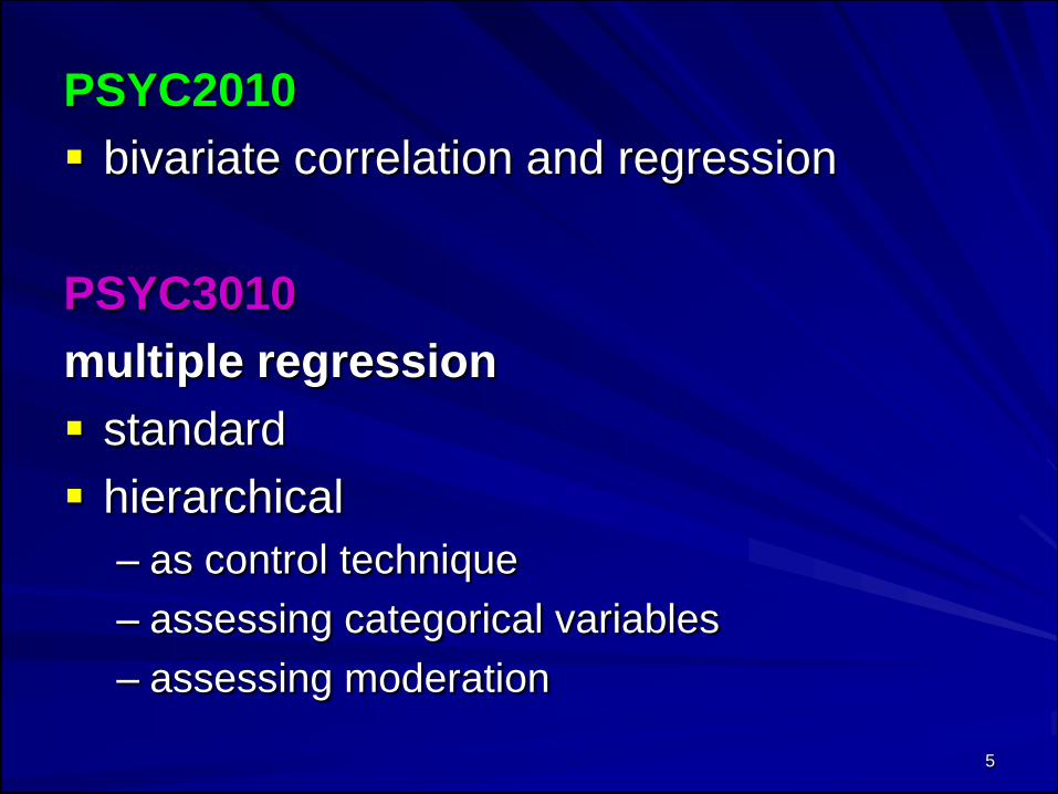
PSYC2010

bivariate correlation and regression

PSYC3010

multiple regression

standard

hierarchical

– as control technique

– assessing categorical variables

– assessing moderation

6

The purpose of statistics To understand the shape of the data

To understand meaningful questionsand assess meaningless ranting– “Women mature faster than men” “Men are

stronger”• What‟s the standard deviation? Is the difference

reliable - Is it even going to be significant in the population?

• What‟s the effect size? What portion of the variance in the data does gender account for?

• What are other factors associated with gender to control for (e.g., via ANCOVA)? [ANOVA is not causation!]

• What other factors might moderate this effect? (interactions!)

7

The purpose of statistics Meaningful ?s and meaningless ranting

– The wealthier you are, the happier you are!• Is that relationship reliable, is it significant in the

population?

• What is the effect size?

• What other factors might need to be controlled for? [Correlation is not causation!]

• What other factors might moderate this effect? (interactions!)

• Is this really a linear effect ?

To read psych articles, need to know statistics –now you can read most & understand them

more broadly, it‟s difficult to understand human variability meaningfully without understanding what variability and differences are and are not.

8

when do you use which

analysis?Need to consider the type of variables:

independent (predictor) and dependent (criterion).

Predictors

Categorical

Categorical & Continuous

Continuous

Continuous

Categorical

Criterion

Continuous

Continuous

Continuous

Categorical

Categorical

Method

ANOVA; MR

MR

MR

Logistic Regression

Log-linear Analysis

9

(2) A bit on logistic regression

If all our acts are conditioned behaviour, then so are our theories:

yet your behaviourist claims his is objectively true.

-- W. H. Auden

10

0

1

2

3

4

5

6

7

8

9

10

0 1 2 3 4 5 6 7 8 9 10

Number of Social Events Attended

Lif

e S

ati

sfa

cti

on

Multiple regression = continuous IVs and DVs,

each normally distributed. We fit the data with a

linear model – the straight line minimising the

discrepancy between Y and Y hat

11

Logistic regression = continuous IVs and categorical (0, 1)

DV. Obviously (a) Y is not normally distributed and (b) a

straight line fits this data poorly.

0

0.1

0.2

0.3

0.4

0.5

0.6

0.7

0.8

0.9

1

0 1 2 3 4 5 6 7 8 9 10


Mo

rtality

wit

hin

5 y

ears

(1=d

ead

)

12

Accordingly we fit the data with a logistic model – the S-

shape curve (a.k.a., sigmoidal curve) that best predicts

whether an observation will be in one group (0) versus

another (1).

0

0.1

0.2

0.3

0.4

0.5

0.6

0.7

0.8

0.9

1

0 1 2 3 4 5 6 7 8 9 10


Mo

rta

lity

wit

hin

5 y

ea

rs (

1=

de

ad

)

13

Conceptual similarities:

Interpreting logistic R2 and R2 change

In SPSS for logistic regression, you get R2 estimates

labelled Cox & Snell R2 and Nagelkerke R2

– These are two ways of understanding the “variance” in

dichotomous (0, 1) DVs

– No convention exists regarding which to report - C&S is the more

conservative one, and Nagelkerke is more liberal – at the

moment Nagelkerke R2 is more common.

Hierarchical logistic regression can be performed

– SPSS will output C&S and N R2 for each model but you need to

subtract the later R2 from earlier to get R2 change / block

R2 and R2 change are tested with chi-square ( χ2 ) tests,

not F-tests, but structure of write-up = identical

Both X2 for model and for block are reported,

R2 change must be calculated by hand from the output.

14

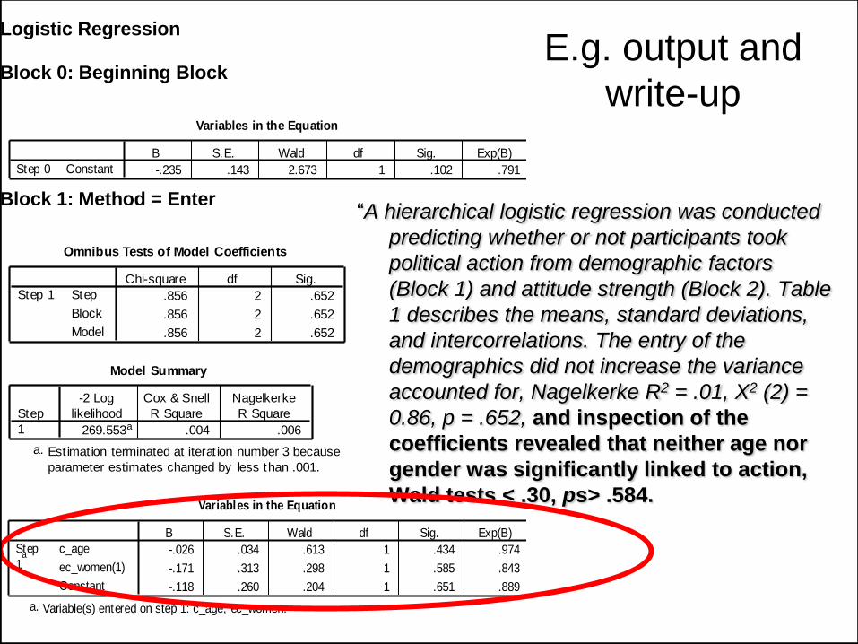
E.g. output and

write-up

Logistic Regression Block 0: Beginning Block

Variables in the Equation

-.235 .143 2.673 1 .102 .791ConstantStep 0

B S.E. Wald df Sig. Exp(B)

Block 1: Method = Enter

Omnibus Tests of Model Coefficients

.856 2 .652

.856 2 .652

.856 2 .652

Step

Block

Model

Step 1

Chi-square df Sig.

Model Summary

269.553a .004 .006

Step

1

-2 Log

likelihood

Cox & Snell

R Square

Nagelkerke

R Square

Est imation terminated at iterat ion number 3 because

parameter estimates changed by less than .001.

a.


-.026 .034 .613 1 .434 .974

-.171 .313 .298 1 .585 .843

-.118 .260 .204 1 .651 .889

c_age

ec_women(1)

Constant

Step

1a


Variable(s) entered on step 1: c_age, ec_women.a.

“A hierarchical logistic regression was conducted

predicting whether or not participants took

political action from demographic factors

(Block 1) and attitude strength (Block 2).

Table 1 describes the means, standard

deviations, and intercorrelations. The entry of

the demographics did not increase the

variance accounted for, Nagelkerke R2 = .01,

X2 (2) = 0.86, p = .652 [snip]

15



14.475 1 .000

14.475 1 .000

15.331 3 .002

Step

Block

Model

Step 1

Chi-square df Sig.

Model Summary

255.078a .075 .100

Step

1

-2 Log

likelihood

Cox & Snell

R Square

Nagelkerke

R Square

Est imat ion terminated at iterat ion number 4 because


a.


-.045 .035 1.622 1 .203 .956

-.054 .327 .028 1 .868 .947

.404 .110 13.439 1 .000 1.498

-1.073 .379 8.015 1 .005 .342

c_age

ec_women(1)

atstr_sc

Constant

Step

1a


Variable(s) entered on step 1: atst r_sc.a.

“However, the entry of attitude strength in

Block 2, significantly increased the variance

accounted for, Nagelkerke R2 change = .09,

X2 (1) = 14.48, p < .001. [snip] The final

model accounted for only 10% of the

variance in action however, X2 (3) = 15.33,

p = .002.

E.g. output

and write-up

Note: the the difference

between 2LL in this model

(255.078) and the first model

(269.553) equals the chi-

square value (14.475).

Some reviewers prefer

reporting 2LL over R2

16

How should we like it were stars to burn

With a passion for us we could not return?

If equal affection cannot be

Let the more loving one be me .

-- W. H. Auden

17

Return to the data…

0

0.1

0.2

0.3

0.4

0.5

0.6

0.7

0.8

0.9

1

0 1 2 3 4 5 6 7 8 9 10


Mo

rta

lity

wit

hin

5 y

ea

rs (

1=

de

ad

)

18

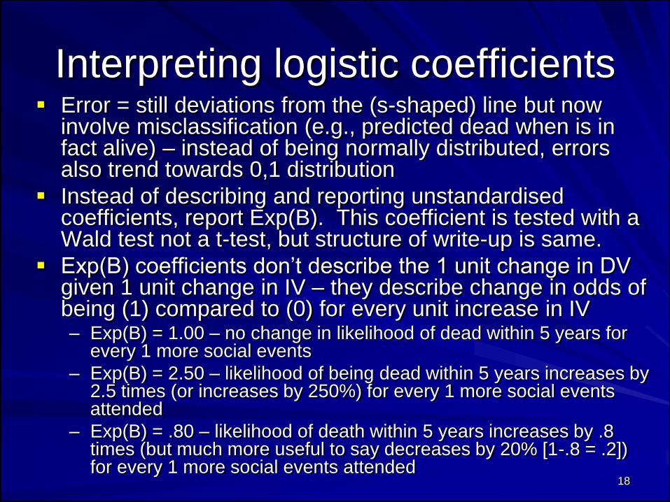
Interpreting logistic coefficients Error = still deviations from the (s-shaped) line but now

involve misclassification (e.g., predicted dead when is in fact alive) – instead of being normally distributed, errors also trend towards 0,1 distribution

Instead of describing and reporting unstandardised coefficients, report Exp(B). This coefficient is tested with a Wald test not a t-test, but structure of write-up is same.

Exp(B) coefficients don‟t describe the 1 unit change in DV given 1 unit change in IV – they describe change in odds of being (1) compared to (0) for every unit increase in IV– Exp(B) = 1.00 – no change in likelihood of dead within 5 years for

every 1 more social events

– Exp(B) = 2.50 – likelihood of being dead within 5 years increases by 2.5 times (or increases by 250%) for every 1 more social events attended

– Exp(B) = .80 – likelihood of death within 5 years increases by .8 times (but much more useful to say decreases by 20% [1-.8 = .2]) for every 1 more social events attended

19

E.g. output and

write-up

Logistic Regression Block 0: Beginning Block


-.235 .143 2.673 1 .102 .791ConstantStep 0




.856 2 .652

.856 2 .652

.856 2 .652

Step

Block

Model

Step 1

Chi-square df Sig.

Model Summary

269.553a .004 .006

Step

1

-2 Log

likelihood

Cox & Snell

R Square

Nagelkerke

R Square

Est imation terminated at iterat ion number 3 because


a.


-.026 .034 .613 1 .434 .974

-.171 .313 .298 1 .585 .843

-.118 .260 .204 1 .651 .889

c_age

ec_women(1)

Constant

Step

1a


Variable(s) entered on step 1: c_age, ec_women.a.

“A hierarchical logistic regression was conducted

predicting whether or not participants took

political action from demographic factors

(Block 1) and attitude strength (Block 2). Table

1 describes the means, standard deviations,

and intercorrelations. The entry of the

demographics did not increase the variance

accounted for, Nagelkerke R2 = .01, X2 (2) =

0.86, p = .652, and inspection of the

coefficients revealed that neither age nor

gender was significantly linked to action,

Wald tests < .30, ps> .584.

20



14.475 1 .000

14.475 1 .000

15.331 3 .002

Step

Block

Model

Step 1

Chi-square df Sig.

Model Summary

255.078a .075 .100

Step

1

-2 Log

likelihood

Cox & Snell

R Square

Nagelkerke

R Square

Est imat ion terminated at iterat ion number 4 because


a.


-.045 .035 1.622 1 .203 .956

-.054 .327 .028 1 .868 .947

.404 .110 13.439 1 .000 1.498

-1.073 .379 8.015 1 .005 .342

c_age

ec_women(1)

atstr_sc

Constant

Step

1a


Variable(s) entered on step 1: atst r_sc.a.

“However, the entry of attitude strength in

Block 2, significantly increased the variance

accounted for, Nagelkerke R2 change = .09,

X2(1) = 14.48, p < .001. Specifically, on a

scale from 0 to 5, every additional unit of

attitude strength increased the

likelihood of political action by 150%,

Exp(B) = 1.50, Wald = 13.44, p < .001.

The final model accounted for only 10% of

the variance in action however, X2 (3) =

15.33, p = .002.”

E.g. output and write-up

21

Logistic regression is seen quite often, e.g.:– clinical psychology (what factors predict becoming

schizophrenic, recurrence of depression?)

– social (predict attending rally, getting divorced?)

– org psych (predict quitting the firm / being promoted?)

Occasionally other statistics are reported but the above would serve in a journal article at the moment.

Also can have multiple categories on DV – Use multinomial logistic regression

So worth knowing

Field spells it all out rather nicely and goes thru SPSS

Covered in Howell section 15.14 (5th & 6th ed)

But not assessed on exam!

Also note: on course outline this week‟s reading and extra tutorial exercise is Log linear (Howell chpt 17) but we won‟t get around to covering this so feel free to ignore (as psychs you will come across logistic regression far more frequently)

22

(3) T-VALS

Knowing artists, you think you know all about Prima Donnas:

boy!, just wait till you hear scientists get up and sing.

-- W. H. Auden

23

(4) Exam Info

24

Structure of the exam 40 multiple-choice questions

– 1 mark each; content spread across the 11 content lectures

2 short answer questions

– 10 marks each; content focuses on key themes of the course: factorial ANOVA (within, between, and/or mixed) and multiple

regression (standard, hierarchical, and/or moderation)– Each short-answer question has a bonus question worth 1 mark

(so in theory could score 11/10) – take a punt if you have time

2 hours working time + 10 mins perusal

– Pace yourself

formula sheet included

– does not include DF calculations

– up on Blackboard now (see “practice exam questions” link)

25

content of exam

primarily conceptual

moving between research questions, design, and hypotheses

partitioning variance

understanding of linear models

understanding of error terms

interpretation of statistics– description of results (e.g., F and p values provided)

– no SPSS output

calculating degrees of freedom

26

preparing for the exam

revise the lecture notes

everything you need to know for the exam can be found in the 12 lectures

read the readings

readings (and tute exercises) will help to consolidate and clarify this material

complete the practice questions

the practice exam (web handouts) and extra practice questions (tute workbook, web handouts) are representative of the kinds of questions you will have to answer

think about what might be asked on the exam

the exam content MC questions are more or less evenly spread across the lectures

The short answer questions target key themes of course – factorial ANOVA (between/ within / mixed) and regression

27

Important Examination Information. Candidates are reminded of the following:

Double-check the examination timetable to ensure you have the correct date, time and venue for your examination.

Be at the examination room at least 15 minutes before the scheduled start time.

Bring your University Identity Card to the examination room. Your identity card must be prominently displayed on your desk. The University will conduct identity checks. You may not be permitted to sit the examination if you do not have your student ID card with you.

You are not permitted to have a mobile telephone on your person during an examination. Please be aware that the use of mobile phone detectors has recently been introduced for examination rooms.

Do not bring anything such as books, notes, calculators etc into the examination room unless they are specifically permitted for that examination and are listed on the examination cover sheet; (Candidates found in possession of unauthorised items in an examination will be liable to investigation for misconduct.)

Bring pens, pencils, rulers, erasers etc. Do not attempt to take your own scrap paper or post-it notes into the examination room.

When you enter the examination venue, sit at the seat number given to you on entry to the exam room.

No food or drinks, other than a small clear bottle of still water with the label removed, can be taken into the examination room.

Leave all personal property, other than writing and drawing instruments in the area specified by the Invigilator. Please note these items are left at the candidate‟s own risk.

Do not bring into the examination room, any item which may cause a disturbance to others, for example an audible alarm watch.

28

Practice exam

10 MC questions, 2 short answer

Answers will be discussed in tutes this

week

29

(5) Interconnections between

ANOVA and regression

30

ANOVA

& t-tests

between/within

Bivariate

(simple)correlation

Factorial

ANOVA

between/within& mixed

Multiple

Regression

…multivariate methods…

31

experimental vs. correlational

research

this is what many will tell you about the differences between anova vs correlational designs:

Anova designs– the only research strategy in which causation can be inferred -

the factor can be said to “cause” changes in DV

– this is because the IV is manipulated

correlational research– can not be used to infer causality

– this is because variables are not manipulated -- just measured

32

experimental vs. correlational

researchthis is misleading because:

it is confuses research methodology (PSYC3042) with statistical methodology (PSYC3010), and it assumes that the benefits of experimental research transfer automatically to anova

- the differences between experimental and correlational research involve random assignment to levels of IV vs observation of natural / measured levels of IV

- These have NOTHING to do with the differences between anova and regression, which involve partitioning variance between factors and within versus between a regression line and observations

- ANOVA can be carried out statistically with regression analyses; t-tests can be carried out with correlations

- All of these statistical techniques are generalisations of one underlying model, the general linear model (GLM)

33

The General Linear Model

What is it?

Xijk = + j + k + jk + eijk

Xij = + j + i + eij

Y = b1X + b2Z + b3XZ + c + e

34

The General Linear Model

What is it?

a system of linear equations

which can be used to model data

quite similar to the T1000:

- powerful!

- versatile!

- can execute a range of operations!

- can take on a variety of appearances!

- provides the basis for just about

every parametric statistical test we

know (OK, weak link there…)

Read Cronbach, 1968 for more

35

he closed his eyes

upon that last picture, common to us all,

of problems like relatives gathered

puzzled and jealous about our dying.

-- W. H. Auden, “In Memory of Sigmund Freud”

36

magic tricks!

it is fairly easy to show that:

1. a t-test is a correlation

2. factorial anova is a standard

regression problem

3. ancova is a hierarchical

regression problem

4. interactions in anova are

identical to those in MMR

37

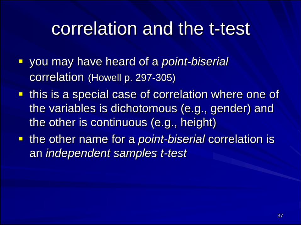
correlation and the t-test

you may have heard of a point-biserial

correlation (Howell p. 297-305)

this is a special case of correlation where one of

the variables is dichotomous (e.g., gender) and

the other is continuous (e.g., height)

the other name for a point-biserial correlation is

an independent samples t-test

38

Females Males

150 165

160 170

165 180

155 175

Heights of males and

females – this is how we

are used to seeing the data

laid out when we are doing

hand calculations for t-test

but we know that SPSS

would prefer that we lay the

data out like this

hmmm…looks familiar…

Gender Height

1 150

1 160

1 165

1 155

2 165

2 170

2 180

2 175

39

so let‟s run our t-test…

Independent Samples Test

.000 1.000 -3.286 6 .017

-3.286 6.000 .017

Equal variances

assumed

Equal variances

not assumed

HEIGHT

F Sig.

Lev ene's Test for

Equality of Variances

t df Sig. (2-tailed)

t-test f or Equality of Means

t(6) = 3.29, p = .017

40

now run as a correlation… (just as if we had two continuous variables)

r = .802, p = .017, r2 = .643

Correlations

1 .802*

. .017

8 8

.802* 1

.017 .

8 8

Pearson Correlation

Sig. (2-tailed)

N

Pearson Correlation

Sig. (2-tailed)

N

GENDER

HEIGHT

GENDER HEIGHT

Correlat ion is signif icant at the 0.05 lev el (2-tailed).*.

p value is the same as in t-test

41

re-run as an anova… (to get estimates of effect size)

F(1,6) = 10.8, p = .017, η2 = .643 p value is again the same

partial η2 = r2 (from previous slide)

F (i.e., 10.8) = t2 (i.e., 3.292)

Tests of Between-Subjects Effects

Dependent Variable: HEIGHT

450.000a 1 450.000 10.800 .017 .643

217800.000 1 217800.000 5227.200 .000 .999

450.000 1 450.000 10.800 .017 .643

250.000 6 41.667

218500.000 8

700.000 7

Source

Corrected Model

Intercept

GENDER

Error

Total

Corrected Total

Ty pe III Sum

of Squares df Mean Square F Sig.

Part ial Eta

Squared

R Squared = .643 (Adjusted R Squared = .583)a.

42

now run as a regression… (just for the sake of comparison)

R2 = .643, F(1,6) = 10.8, p = .017

Model Summary

.802a .643 .583 6.45497

Model

1

R R Square

Adjusted

R Square

Std. Error of

the Estimate

Predic tors : (Constant), GENDERa.

ANOVAb

450.000 1 450.000 10.800 .017a

250.000 6 41.667

700.000 7

Regression

Residual

Total

Model

1

Sum of

Squares df Mean Square F Sig.

Predictors: (Constant), GENDERa.

Dependent Variable: HEIGHTb.

R2 = partial e2 = r2

F and p are

the same…

43

an additional slide to consolidate

structural modelsFirst to help interpretation re-run MR using dummy coding (female = 1 male

= 0) Can use structural model to calc means:

Group Statistics

4 172.5000 6.45497 3.22749

4 157.5000 6.45497 3.22749

gender

male

f emale

height

N Mean Std. Dev iat ion

Std. Error

Mean

From t-test

Coefficientsa

172.500 3.227 53.447 .000

-15.000 4.564 -.802 -3.286 .017

(Constant)

gender

Model

1

B Std. Error

Unstandardized

Coeff icients

Beta

Standardized

Coeff icients

t Sig.

Dependent Variable: heighta.

From regress

Y hat = a + B1X 1

So, for men (coded as zero), Y hat = 172.50 – (15.00*0) = 172.50

And for women (coded as one), Y hat = 172.50 – (15.00*1) = 157.50

44

explanation

a t-test, or an anova between two groups, is just a special case of correlation, – which in turn is just a special case of regression,

– which is a representation of the General Linear Model

SPSS did the same* thing in all four analyses –it just presented the output in different ways

*(strictly speaking, bivariate correlations and t-tests are not executions of the GLM – they are calculated using „shortcuts‟ that achieve the same basic results)

45

hierarchical regression and ancova

in ancova our goal was to remove the effects of a covariate before examining our treatment effect

in hierarchical regression, the idea was to examine the contribution of a set of variables at step 2 after accounting for prediction at step 1– as it turns out, both are basically doing the same

thing!

46

let‟s go back to

our height data

– and include

age as a

covariate:

data is laid out how we

would for an ancova or a

hierarchical regression

Sex Age Height

1 16 150

1 18 160

1 17 165

1 17 155

2 16 165

2 17 170

2 18 180

2 17 175

47



606.250a 2 303.125 16.167 .007 .866

47.690 1 47.690 2.543 .172 .337

156.250 1 156.250 8.333 .034 .625

450.000 1 450.000 24.000 .004 .828

93.750 5 18.750

218500.000 8

700.000 7

Source

Corrected Model

Intercept

AGE

GENDER

Error

Total

Corrected Total

Ty pe III Sum

of Squares df Mean Square F Sig.

Part ial Eta

Squared


first run as an ancova …

for gender, F(1,5) = 24.00, p = .004

this is the effect after controlling for age

48

Model Summary

.472a .223 .223 1.724 1 6 .237

.931b .866 .643 24.000 1 5 .004

Model

1

2

R R Square

R Square

Change F Change df 1 df 2 Sig. F Change

Change Statist ics

Predic tors : (Constant), AGEa.

Predic tors : (Constant), AGE, GENDERb.

now run as hierarchical regression…

Fch(1,8) = 24.00, p = .004

this is the effect after controlling for age

49

Minor diffs in output

there are some minor differences in presentation:

– in our ancova we are given η2 = .828 but in regression

the R2ch was .643

– η2 actually corresponds to the squared partial

correlation for gender .912 = .828

Coefficientsa

.725 .496

.472 1.313 .237 .472 .472

.976 .374

.472 2.887 .034 .791 .472

.802 4.899 .004 .910 .802

(Constant)

AGE

(Constant)

AGE

GENDER

Model

1

2

Beta

Standardized

Coeff icients

t Sig. Part ial Part

Correlat ions

Dependent Variable: HEIGHTa.

50

Minor diffs in output

– in our ancova the test for age is given as F(1,5) =

8.33, p = .034

– this actually corresponds to the test of the coefficient

for age in the full model at step 2:

• remember t2 = F (2.8872 = 8.33)

Coefficientsa

.725 .496

.472 1.313 .237 .472 .472

.976 .374

.472 2.887 .034 .791 .472

.802 4.899 .004 .910 .802

(Constant)

AGE

(Constant)

AGE

GENDER

Model

1

2

Beta

Standardized

Coeff icients

t Sig. Part ial Part

Correlat ions

Dependent Variable: HEIGHTa.

51

explanation

ancova and hierarchical regression achieve the same broad purpose

some minor differences in the output simply reflect defaults which have been programmed into SPSS – e.g., as effect sizes have only recently become

emphasised for anova, these don‟t line up as you would expect with the ones for regression, but the link is in there somewhere!

52

interactions – MMR vs anova

testing interactions in anova and MMR

look incredibly different

– this is just because they have different

histories

– essentially they are doing the same thing

53

2 categorical variables

going back to our height data, let‟s say we

wanted to examine the interaction

between maternal diet and gender in the

prediction of height…

– factor A is gender (M/F)

– factor B is maternal diet (healthy, unhealthy)(N = 16)

54



950.000a 3 316.667 8.444 .003

435600.000 1 435600.000 11616.000 .000

625.000 1 625.000 16.667 .002

100.000 1 100.000 2.667 .128

225.000 1 225.000 6.000 .031

450.000 12 37.500

437000.000 16

1400.000 15

SourceCorrected Model

Intercept

GENDER

DIET

GENDER * DIET

Error

Total

Corrected Total

Ty pe III Sum

of Squares df Mean Square F Signif icance


anova – the way we know…

F (1,12) = 6.00, p = .031

55

MMR…

in our MMR lecture we talked briefly about

categorical variables in MMR – they can

get a bit tricky

but with dichotomous variables it is dead

easy

– enter additive effects (gender and diet) at step

1

– interaction term (gender*diet) at step 2….

56

MMR…

Model Summary

.720a .518 .444 7.20577 .518 6.981 2 13 .009

.824b .679 .598 6.12372 .161 6.000 1 12 .031

Model

1

2

R R Square

Adjusted

R Square

Std. Error of

the Estimate

R Square

Change F Change df 1 df 2

Signif icance F

Change

Change Statist ics

Predic tors: (constant) DIET, GENDER...a.

Predic tors: (constant) DIET, GENDER, INT...b.

Fch (1,12) = 6.00, p = .031

57

implications

the GLM has been behind the scenes for just about all of the statistical methods examined in PSYC3010

we stick to a lot of these conventions about when to use ANOVA instead of regression for practical reasons

by understanding the common links through all these analyses we can be less rigid in our use of these tools

here are some of the comparisons we can make

58

hypothesis testing

in anova we test the hypothesis that our manipulations have had a significant effect on our DV

H0: 1 = 2 = 3

– the null hypothesis – no differences among treatment means

H1: the null hypothesis is false– the alternative hypothesis – there is at least one difference among

treatment means

in regression we test the hypothesis that our predictors are accounting for a significant amount of variance in our criterion

H0: the relationship between the criterion and the set of predictors is zero

H1: the relationship between the criterion and the set of predictors isnot zero

59

variance partitioning

in anova we want to partition the total variance out into effects and error terms– main effects and interactions compared to error

– the goal is to attribute a significant and substantial proportion of variance in our DV to our effects

in regression we want to model our data by finding the line/plane of best fit, i.e., the one that minimises errors of prediction– the model can then be described in terms of additive effects

and interactions, which are compared to error

– the goal is to explain a significant and substantial proportion of variance in our criterion as possible

60

effect size

in anova we can quantify the amount of the total variance which each effect accounts for– eta-squared (sample estimate)

– omega-squared (population estimate)

in regression we can quantify the amount of variance that our model accounts for– R2 (sample estimate)

– R2 adjusted (population estimate)

– sr2 (importance of individual predictor)

61

complex relationships

in anova we can test for 2-way or 3-way interactions (and beyond!)– the effect of factor A on the DV changes over levels of factor B

– follow-up these with simple effects – i.e., examine the effect of A on the DV at each level of B

in regression we can test for 2-way or 3-way interactions (and beyond!)– the relationship between X and Y varies over values of Z

– follow-up these with simple slopes – i.e., examine the relationship between X and Y at high and low conditional values of Z

62

increasing power

in anova we can employ a number of statistical and methodological techniques: – blocking on a concomitant factor

– remove individual differences (i.e., use a within-subjects design)

– include a covariate (i.e., use ancova)

in regression we also have some similar techniques at our disposal:– partial the effect of another variable out first (i.e., use hierarchical

regression - similar to ancova)

– improve measurement (e.g., measure subjects with most reliable measures – i.e., higher alpha)

63

The multivariate universe:

Before 3010:– Single explanations

– Barely grasp difference between correlations and group differences

– Tendency to rely too much on p-values

After 3010:– Multiple explanations

– Explanations that interact, or are inter-related

– Variables considered jointly so you can see interactions and inter-relationships explain more than considering each alone

– Strong understanding of correlations and group differences

– Understanding key idea of effect sizes

64

In the tutes:

This week: Practice exam

In future :

Consult times for me for the exam will be Friday November 7th 11am-12 and 1-2pm or by appointment– Not available on weekends – please go through

materials & ask questions ahead of time!

Every effort will be made to post the A2 marks online by Friday November 7th, although this cannot be guaranteed

Documents

psyc3010 lecture 12 - UQ Psychology