PSEUDOSPECTRAL SOLUTION OF NEAR …people.ku.edu/~wzhuang/research/paper/MHS98.pdf · PSEUDOSPECTRAL SOLUTION OF NEAR-SINGULAR PROBLEMS USING NUMERICAL COORDINATE TRANSFORMATIONS

PSEUDOSPECTRAL SOLUTION OF NEAR-SINGULAR PROBLEMSUSING NUMERICAL COORDINATE TRANSFORMATIONS BASED

ON ADAPTIVITY∗

L. S. MULHOLLAND† , W.-Z. HUANG‡ , AND D. M. SLOAN†

SIAM J. SCI. COMPUT. c© 1998 Society for Industrial and Applied MathematicsVol. 19, No. 4, pp. 1261–1289, July 1998 012

Abstract. The work presented here describes a method of coordinate transformation thatenables spectral methods to be applied efficiently to differential problems with steep solutions. Theapproach makes use of the adaptive finite difference method presented by Huang and Sloan [SIAMJ. Sci. Comput., 15 (1994), pp. 776–797]. This method is applied on a coarse grid to obtain a roughapproximation of the solution and a suitable adapted mesh. The adaptive finite difference solutionpermits the construction of a smooth coordinate transformation that relates the computational spaceto the physical space. The map between the spaces is based on Chebyshev polynomial interpolation.Finally, the standard pseudospectral (PS) method is applied to the transformed differential problemto obtain highly accurate, nonoscillatory numerical solutions. Numerical results are presented forsteady problems in one and two space dimensions.

Key words. adaptivity, equidistribution, pseudospectral, differential equations

AMS subject classifications. 65N35, 65N50, 76D30

PII. S1064827595291984

1. Introduction. PS methods provide an attractive alternative to finite differ-ence and finite element methods for numerical solution of differential equations. ThePS method involves approximation by global basis functions—trigonometric or alge-braic polynomials, for example—whereas finite difference and finite element methodsinvolve local approximations. For problems with smooth solutions the convergencerate of PS methods is faster than algebraic as the number of grid points increases, andthe significance of this so-called spectral convergence is that a specified accuracy canusually be achieved using fewer grid points than would be required by the algebraicallyconvergent finite difference or finite element approaches. However, if a solution has asteep region such as a boundary layer or an interior layer the PS method will achievehigh accuracy only if the number of grid points is sufficiently high to permit resolu-tion of the localized phenomena. The required number can be prohibitive in practice,and if insufficient grid points are used an inaccurate numerical solution contaminatedby global oscillations will result. In situations of this type a PS method will not becompetitive with local approximation methods.

Various schemes have been proposed for improving spectral or PS approximationsof steep or discontinuous solutions. The schemes might well be classified into twogroups that treat dependent and independent variables, respectively.

Remedial action on dependent variables usually involves the addition of some formof artificial viscosity or the application of postprocessing such as filtering. Examplesof filtering applied to spectral approximation of discontinuous solutions may be foundin the papers by Majda, McDonough, and Osher [21]; Gottlieb, Lustman, and Orszag

∗Received by the editors August 23, 1995; accepted for publication (in revised form) September30, 1996; published electronically April 16, 1998.

http://www.siam.org/journals/sisc/19-4/29198.html†Department of Mathematics, University of Strathclyde, Glasgow G1 1XH, Scotland

([email protected], [email protected]). The first author was supported by the Engineer-ing and Physical Sciences Research Council (EPSRC).

‡Department of Mathematics, University of Kansas, Lawrence, KS 66045 ([email protected]).

1261

1262 L. S. MULHOLLAND, W.-Z. HUANG, AND D. M. SLOAN

[12]; and Cai, Gottlieb, and Shu [7], [8]. The vanishing viscosity method proposed byTadmor for shock capturing is described in [23, 24, 25]. All of these methods producespectral accuracy in smooth regions between discontinuities, with each discontinuitygenerally confined to one grid interval. Recently, Huang and Sloan [17] proposedan upwind PS method for singular perturbation problems without turning points.This upwind method is shown to be free of oscillations and spectrally accurate as thenumber of grid points tends to infinity, with the perturbation parameter held fixed.

Methods that deal with treatment of the independent variable are applicable toproblems with steep, but smooth, solutions. Here, the usual approach is to apply acoordinate transformation that is designed to smooth out regions of high gradient.In the transformed coordinate a PS method can yield spectral accuracy using a rea-sonably small number of grid points. A transformation that adapts to the featuresof a solution—usually constructed as the solution is being generated numerically—isthe basis of adaptive grid generators. This has been used to great effect with finitedifference and finite element methods (for example, see [6], [10], [15], [18], [26], [27],[28]). A common theme in adaptive finite difference and finite element methods is theconcept of equidistribution, which seeks to distribute some function evenly over thedomain of the problem. The function is usually some measure of computational erroror solution variation. The paper by Huang and Sloan [18] gives an interpretation ofequidistribution in the context of adaptive grid generation for multidimensional prob-lems. An equidistribution principle is developed in [18] and it is used to formulate afinite difference grid generation algorithm in two space dimensions.

Adaptive schemes have so far not been extended in a widely applicable formula-tion to spectral or PS approximation methods. In this paper we show how adaptivitybased on equidistribution may be incorporated into PS discretization of problems inone space dimension. We also show how to improve the effectiveness of PS methodsfor steep solutions in one and two dimensions by adapting a coordinate transformationto a quickly computed finite difference solution. A highly accurate PS solution is thenobtained in the transformed coordinate. Adaptively generated coordinate transfor-mations have been used previously in PS computations. In [1] this approach is usedto solve problems with steep, but continuous, solutions and a coordinate transforma-tion is coupled with artificial viscosity to solve shock wave problems. An analogoustechnique is adopted in [2], [3], [4], [5], and [14] to solve the Burgers equation, reac-tion diffusion equations, and flame propagation problems. In each of these papers thecoordinate transformation is represented as a parameterized function whose structureis known a priori. The parameter values are obtained by minimizing a functional thatmeasures some error in the computed solution: for example, the functional might berelated to the interpolation error. For a specified number of grid points the accuracyobtained in the transformed coordinate is much higher than that which would resultfrom direct PS solution in the physical coordinate. Note that, in general, polynomialapproximation in the transformed coordinate corresponds to approximation in thephysical coordinate by means of basis functions that are not polynomials. It is theuse of basis functions resulting from the mapping that gives rise to the high accuracyof the computed solution.

A parameterized transformation containing a small number of parameters—asused in [2], [3], [4], [5], and [14]—is only effective if prior knowledge of the solution isavailable. For example, the prior knowledge might be information on the locations offronts. Here we remove the need for prior knowledge by using parameterized functionscontaining many parameters, with information on the features of the solution gener-

ADAPTIVE PSEUDOSPECTRAL METHOD 1263

ated by means of a low-cost adaptive finite difference method. Since the knowledgeof the solution is generated numerically the features of the solution are not needed apriori, and the method is thus widely applicable.

The objectives of this paper are to show that adaptivity may be coupled withPS discretization to produce highly accurate solutions to problems that have steep,smooth solutions. We show how a postprocessing PS discretization may be appliedto adaptive finite difference solutions, computed quickly on coarse grids, to producehighly accurate results at little extra cost. The PS discretization is applied to asystem that has the same degree of nonlinearity as the physical system. For example,if the physical PDE is linear, then the PS discrete equations are linear. Section 2extends the finite difference adaptive method of Huang and Sloan [18] to deal with PSdiscretization in one space dimension. In section 3 we use the adaptive finite differencescheme in [18] to produce an approximation of the solution and an adapted mesh inthe physical coordinate: here a coarse mesh suffices to give a solution that need not behighly accurate. Polynomial interpolation is then used to obtain approximations tothe physical mesh at Chebyshev nodes, and a coordinate transformation is obtained byfitting a Chebyshev polynomial expansion to these nodal values. Finally, a standardPS method is employed to solve the transformed differential equation. The processis presented for problems in one space dimension in section 3 and for two spacedimensions in section 4, and in each of these sections numerical results are describedfor steady problems with near-singular solutions. Section 5 contains conclusions andcomments on our PS adaptive algorithms.

2. PS adaption based on equidistribution.

2.1. Formulation of algorithm. In [18] the concept of equidistribution is usedto generate a one-to-one coordinate transformation from the computational domainDc to the physical domain Dp in the form

x = x(ξ), ξ ∈ Dc ⊂ Rm.(2.1)

The determination of a mesh, or distribution of nodes, on Dp is equivalent to theconstruction of a (discrete) transformation (2.1). The presentation by Huang andSloan shows how an equidistribution principle may be used to determine a distributionof nodes on Dp that corresponds—under the transformation (2.1)—to a given uniformmesh on Dc.

In this section we give the obvious PS extension of the algorithm in [18]: a (dis-crete) transformation (2.1) is constructed that determines a distribution of nodes onDp corresponding to a set of Chebyshev–Gauss–Lobatto nodes on Dc. For simplic-ity we present the PS adaptive method for steady differential problems in one spacedimension, in which case the map (2.1) takes the form

x = x(ξ), ξ ∈ [−1, 1].(2.2)

Without loss of generality we assume that x ∈ [−1, 1] ⊂ R under (2.2), with

x(−1) = −1, x(+1) = +1.(2.3)

Consider the linear boundary value problem ε

d2u

dx2− p(x)

du

dx− q(x)u = f(x), x ∈ (−1, 1),

u(−1) = a, u(+1) = b,(2.4)


where ε > 0 is a small constant (ε � 1) and p, q, and f are smooth functions. (Itwill be obvious in the sequel that more general linear and nonlinear boundary valueproblems may be dealt with in an analogous manner.) If x is related to a coordinateξ ∈ Dc = [−1, 1] by the transformation (2.2) and (2.3), and if v(ξ) = u(x(ξ)), we maywrite equation (2.4) with independent variable ξ in the form

ε

(xξ)2d2v

dξ2−[p(x(ξ))

xξ+

εxξξ(xξ)3

]dv

dξ− q(x(ξ))v = f(x(ξ)), ξ ∈ (−1, 1),

v(−1) = a, v(+1) = b,

(2.5)

where xξ ≡ dxdξ . If x = x(ξ) is chosen such that v(ξ) is slowly varying, the PS approx-

imation of (2.5) will exhibit spectral accuracy. To obtain an effective transformation(2.2) we need to make use of information concerning the features of the solution of(2.4). Here we input the essential information by ensuring that a monitor functionbased on scaled arc length be equally distributed throughout the physical domain Dp

[18].Following [18] we use the monitor function

M(x, u) = 1 + α2

(du

dx

)2

,(2.6)

where α is a real parameter. The condition that M be equally distributed betweennodes in Dp that correspond one-to-one with Chebyshev–Gauss–Lobatto nodes in Dc

is readily shown to be

√1− ξ2 M

12 xξ = constant.(2.7)

(2.7) is a reformulation of equation (16) in [18], with the nodes in the ξ coordinatenow distributed at Chebyshev locations. The aim now is to obtain a PS solution ofthe coupled equations (2.5) and (2.7), making use of the boundary conditions (2.3)and the monitor function representation (2.6).

There are several possible discretizations of the mesh equation (2.7). The onethat we eventually adopted is obtained by squaring (2.7) then differentiating withrespect to ξ. This procedure gives

xξ[(1− ξ2)xξξ − ξxξ] + α2vξ[(1− ξ2) vξξ − ξvξ] = 0,(2.8)

where we have used the transformed monitor function

M = 1 + α2( vξxξ

)2

.(2.9)

Equations (2.3), (2.5), and (2.8) are solved by PS discretization to yield approxima-

tions {xi}Ni=0 and {vi}Ni=0 at the Chebyshev nodes

ξi = − cosπi

N, i = 0, 1, . . . , N,(2.10)

where N is a positive integer and α is set to some preselected value. Approximationsto derivatives at node ξi are computed as summations of the form

(xξ)i =N∑j=0

D(1)ij xj , (xξξ)i =

N∑j=0

D(2)ij xj ,(2.11)


where D(1) and D(2) are, respectively, the first-order and second-order PS differenti-ation matrices corresponding to the nodes (2.10). The reader is referred to references[9] and [11] for information on PS solutions.

The nonlinear algebraic system in 2(N − 1) unknowns arising from the PS dis-cretization of (2.3), (2.5), and (2.8) is solved using a Newton–Raphson iteration withexact representation of the Jacobian, and with continuation in the parameters α andε. The parameter ε is set to a value ε ∼ 1 and a family of problems is solved on thecontinuation path [0, ε] → [α, ε], with the arc-length scaling parameter increasing bysmall steps from 0 to α. A second family of problems is then solved on the continua-tion path [α, ε] → [α, ε], with the diffusion parameter decreasing by small steps fromε to ε. The discrete system with ε << 1 may have a number of unstable solutions. Byemploying continuation in ε from the relatively large value—where there is only one(stable) solution for prescribed α—the path of the stable solution can be followed.The implementation of the continuation process involved a step length, initially set tosolve in one step, reduced by a factor 4 on failure of the Newton–Raphson method andincreased by a factor 1.1 on successful convergence. The Newton–Raphson methodwas deemed to have failed if the residual increased on successive iterations or wheneight iterations were performed without convergence to a required tolerance.

If the equations are solved in the manner described above the mesh quality maybe poor. In particular, for this one-dimensional situation, it is possible that nodecrossing will occur. This corresponds to a situation where the transformation (2.2)is not strictly monotonic increasing in some subregion of [−1, 1]. To avoid this typeof difficulty it is necessary to incorporate some smoothing into the solution process.This has been discussed, for example, in [10] and [18] and an analysis is given in [16].

The smoothing introduced here is achieved by introducing filtering during theevaluation of PS derivative approximations as in equations (2.11). Derivative filteringis readily achieved by modifying the appropriate PS differentiation matrix, and forthis purpose it is convenient to consider a factorized form of the matrix. Suppose afunction v is approximated by the Nth degree polynomial expressed as

v(ξ) ∼ vN (ξ) =N∑n=0

an Tn(ξ),(2.12)

where Tn is a Chebyshev polynomial of the first kind of degree n. If the coeffi-

cients{an}Nn=0

are chosen such that v(ξi) = vN (ξi) for i = 0, 1, . . . , N , then a =

[a0, a1, . . . , aN ]T is related to vN = [vN (ξ0), vN (ξ1), . . . , vN (ξN )]T by the linear rela-tion

vN = C−1 a or a = C vN ,(2.13)

where C is the discrete Chebyshev transform matrix. The first derivative of v isapproximated by

dvNdξ

=N∑n=0

b(1)n Tn(ξ),(2.14)

where the properties of Chebyshev polynomials enable us to relate

b(1) = [b(1)0 , b

(1)1 , . . . , b

(1)N ]T to a as (see [13])

b(1) = E(1) a.(2.15)


The vector that approximates the first-order derivative of v at the nodes{ξi}Ni=0

isgiven by

v(1)N =

[dvNdξ

(ξ0),dvNdξ

(ξ1), . . . ,dvNdξ

(ξN )]T,

and it is readily seen from (2.13)–(2.15) that this is

v(1)N = C−1 E(1) C vN .(2.16)

The matrix C−1 E(1) C is the first-order PS differentiation matrix D(1) introduced in(2.11). Higher-order differentiation matrices have the structure

D(r) = C−1 E(r) C, r = 2, 3, . . . ,(2.17)

where E(r) is readily determined [13]. Alternative views of D(r) are described in thereview by Fornberg and Sloan [11].

Filtering may be included in the differentiation process by modifying D(r) to

D̃(r) = C−1 E(r) BC,(2.18)

where B is a diagonal matrix with elements Bii = βi, i = 0, 1, . . . , N . In this sectionwe have adopted an exponential filter of the form

βi = exp[−δ(i/N)γ ] with δ = 32.(2.19)

Note that β0 = 1, 0 < βi < 1 for i = 1, 2, . . . , N , and βi ≈ 0 for i close to N . Theeffect of introducing B in (2.18) is to diminish the magnitudes of the high componentsin the expansion (2.12) prior to the differentiation process. Filtering may be includedin the approximations to xξ, xξξ, vξ, vξξ in (2.5), (2.8).

2.2. Illustrative examples. We now apply the above algorithm to four sim-ple test problems: three linear and one nonlinear. In each case the same filteringstrategy has been employed: the differentiation matrix D̃(r), given by (2.18), is usedfor the evaluation of vξ and vξξ in (2.8), and for the evaluation of xξ and xξξ in thetransformed differential equation to be solved.

Example 2.1. Consider the linear boundary value problem ε

d2u

dx2+ 2x

du

dx= 0, x ∈ (−1, 1),

u(−1) = −1, u(1) = 1.(2.20)

Given that the exact solution of (2.20) will be very close to u(x) = erf(x/√ε), we

note that for small ε this variable coefficient problem has a steep front at x = 0.

Upon transformation, the term ε d2udx2 becomes ε

xξ(vξxξ

)ξ, with the ith component in the

discrete system given by ε(xξ)i

∑Nk=0 D

(1)ik (

vξxξ

)k. The same discretization procedure is

adopted for the identical second derivative term in Examples 2.2–2.4.We use problem (2.20) to first illustrate the necessity for some form of grid adap-

tion when applying a PS method to approximate solutions with steep gradients. Fig-ure 1a plots the standard PS method approximation for the solution of (2.20) withε = 0.0002, using N = 32. The corresponding adaptive PS approximation, with meshadaption parameter α = 0.5 and filter parameter γ = 10, is plotted in Figure 1b and


-1.5

-1

-0.5

0

0.5

1

1.5

-1 -0.5 0 0.5 1

u

x

(a) Standard PS method

approx.exact

-1.5

-1

-0.5

0

0.5

1

1.5

-1 0 1

u (o

r x)

x (or ξ)

(b) Adaptive PS method

approx: u(x)map: x(ξ)

Fig. 1. Standard and adaptive PS solutions of (2.20) with ε = 0.0002 and N = 32.

0.055

0.06

0.065

0.07

0.075

0.08

0.085

8 14 20 26 32

max

imum

err

or

filter parameter, γ

Adaptive PS error

Fig. 2. Maximum absolute errors versus filter parameter γ for adaptive PS solutions to (2.20)with ε = 0.0002, α = 0.5, and N = 32.

shows that the grid adaption effectively removes the large oscillations by sufficientlyresolving the steep front. Figure 1b also plots the mapping x(ξ) used implicitly in theadaptive PS method; we note that the value of xξ(ξ), though positive throughout, isvery small in a small neighborhood of x = 0.

To show the effect of the filter parameter γ on the error in approximation of theadaptive PS method, Figure 2 plots the maximum absolute error against a range ofvalues of γ. For smaller values of γ the filter becomes too strong for steep fronts tobe sufficiently resolved: the continuation method halts before ε has been reduced aslow as 0.0002. For larger values of γ the filter becomes too weak to dampen out smalloscillations in x(ξ) resulting in a loss of monotonicity: grid crossing is observed. Thefigure shows that within the range of permissible values of γ, the maximum error doesnot vary substantially.

Although the adaptive PS method appears to improve on the standard PS methodfor solving (2.20) given moderately small values of ε, it fails for values of ε much below0.0002. A finite difference method, on the other hand, can provide (see section 3)results of a similar accuracy for much smaller values of ε.

Example 2.2. We now consider a problem obtained by modifying Example 2.1 so


that the solution has a nonzero gradient outside the front for small ε. This is ε

d2u

dx2+ x

du

dx= −επ2 cos(πx)− πx sin(πx), x ∈ (−1, 1),

u(−1) = −2, u(1) = 0.(2.21)

For this problem, the adaptive PS method performs no better than the standard PSmethod for values of ε down to 0.001 and does not converge at all for smaller valuesof ε.

Example 2.3. The linear boundary value problem ε

d2u

dx2+ 2x

du

dx= − 2√

πε

[e−(x+0.5)2/ε − e−(x−0.5)2/ε

], x ∈ (−1, 1),

u(−1) = −2, u(1) = 2

(2.22)

has steep fronts at x = ±0.5 for small ε.The results for this problem are very similar to those of Example 2.2. The adaptive

PS method performs no better than the standard PS method.Example 2.4. The final illustration in this subsection is the nonlinear boundary

value problem ε

d2u

dx2− d(u2)

dx= 0, x ∈ (−1, 1),

u(−1) = 1, u(1) = −1.(2.23)

In this case the steep front, situated at x = 0, has width of order ε, whereas in thethree previous examples the width was of order

√ε. Figure 3 plots the transformation

x(ξ), the monitor function (scaled to have maximum value 1) in computational space,and the computed solution, for ε = 0.01, in physical and computational space, usingN = 32, α = 1, and γ = 10. The maximum absolute error in this case is 4.440× 10−2

compared with an error of 0.678 for the standard PS method. Note that the effectof filtering uξ in the mesh equation is to allow contributions from higher derivativesuξξ, uξξξ, etc. to the computed monitor function [22]. This effect is desirable withrespect to uξξ for the better resolution of x(ξ), where xξ is varying rapidly, but is lessdesirable with respect to higher derivatives. Unfortunately, the filtering process usedhere cannot be that selective.

The numerical experiments described above led us to conclude that simultaneoussolution of discretized forms of (2.5) and (2.8) has its drawbacks. For example, in anextremely steep region the map x = x(ξ) may have ripples that destroy monotonicity,and this gives rise to node crossing. To avoid this, extreme care is needed in intro-ducing filtering. Furthermore, the effort expended in finding a very accurate solutionof the mesh equation (2.8) reduces the computational efficiency of this approach, par-ticularly if one wished to apply it to multidimensional problems. A high accuracy isnot required for the node locations. In the next section we present a method thatovercomes some of these problems.

3. Adaptive transformation method in one dimension.

3.1. Adaptive finite difference method. Here we give a brief description ofthe adaptive finite difference method that is used in the construction of the one-to-one coordinate transformation between the physical and computational domains. Themethod is a one-dimensional formulation of the equidistribution method described in


-1

-0.5

0

0.5

1

-1 0 1

u [o

r x]

x (or ξ)

Adaptive PS method

physical solution: u(x)transformation: x(ξ)

mapped solution: u(ξ)scaled monitor: M(ξ)

Fig. 3. Map, monitor function and adaptive PS solution of (2.23) with ε = 0.01 for N = 32,α = 1, and γ = 10.

[18]. Suppose the aim is to solve equation (2.4). We assume that a transformationx = x(η) is required relating physical nodes

{xi}ni=0

in Dp = [−1, 1] and evenly spacednodes

ηi = −1 +2i

n, i = 0, 1, . . . , n(3.1)

in Dc = [−1, 1]. The equidistribution principle is expressed as

[M x2

η

] 12

= constant,(3.2)

where M is the scaled arc-length monitor function

M = 1 + α2(wη

xη

)2

(3.3)

introduced in (2.6), and w(η) = u(x(η)). Equation (3.2) is approximated at ηi+1/2 bysecond-order central finite differences to give

[M

i+12

(xi+1 − xiηi+1 − ηi

)2] 1

2= constant, i = 0, 1, . . . , n− 1,

where

Mi+

12

= 1 + α2(wi+1 − wi

xi+1 − xi

)2

and xi = x(ηi), wi = u(xi). As in [18] we eliminate the constant and obtain thesystem

[M

i− 12

(xi − xi−1

ηi − ηi−1

)2] 1

2 −[M

i+12


)2] 1

2= 0, i = 1, 2, . . . , n− 1.(3.4)


To obtain a smooth mesh we make use of smoothed matrices

M̃i+

12

=

i+p∑k=i−p

Mk+

12

( q

q + 1

)|k−i|i+p∑

k=i−p

( q

q + 1

)|k−i| ,(3.5)

where the positive real number q is the smoothing parameter and the nonnegativeinteger p is the smoothing index [18]. In (3.5) the summations contain only thoseelements that are well defined (0 ≤ k ≤ n − 1). The discretized grid equation maynow be written as

[M̃

i− 12

(xi − xi−1

ηi − ηi−1

)2] 1

2 −[M̃

i+12


)2] 1

2= 0,

for i = 1, 2, . . . , n− 1,with x0 = −1 and xn = +1.

(3.6)

This grid system is augmented by a finite difference approximation of the differ-ential equation (2.4). This is obtained by first transforming to the computationalcoordinate—to give an equation akin to (2.5), with v and ξ replaced by w and η,respectively—and then discretizing on the uniform mesh by three-point upwind andcentral finite differences for the first and second derivatives, respectively. It should benoted that central differences may be used to approximate the first-order derivative

within the adaptive algorithm. The resulting nonlinear algebraic system in{xi}n−1

i=1

and{ui}n−1

i=1is solved by Newton iteration with exact Jacobian and continuation in

α and ε as described immediately below equation (2.11).Note the effect of the smoothing index p on the structure of the Jacobian in

the Newton iteration. The linearization of (3.6) gives rise to a linear (3 + 2p) blockdiagonal system, where each block is 2 × 2. As p increases the smoothness of themesh increases, and mesh points tend to move out from steep regions to the adjacentregions of high curvature. Note, of course, that the matrices to be inverted in theNewton iteration become more dense as p is increased. To obtain a high quality meshit is essential to find a balance between the tendency of increasing α2 to pull meshpoints into a steep region and the tendency of increasing p to move mesh points outfrom a steep region.

3.2. Construction of coordinate transformation. The previous section pro-vides a discrete transformation that relates the physical mesh

{xi}ni=0

to an evenly

spaced mesh{ηi}ni=0

on Dc. We now use this information to provide a smooth trans-formation like (2.2) that will take u in (2.4) to a suitably slowly varying v in (2.5). Weseek a transformation x = x(ξ) relating the computational and physical domains thatsatisfy some essential properties. To ensure that the map is differentiable and readilycomputable we shall approximate x = x(ξ) by a real polynomial Pm(ξ), where thedegree m need not be set equal to n. To prevent node crossing in Dp we could imposethe severe monotonicity condition P ′

m(ξ) > 0 ∀ξ ∈ [−1, 1]. In principle, this can beachieved by a least squares approach, but it gives rise to a very unwieldy system ofequations in the parameters that define Pm. The conditions imposed effectively ensurethat P ′

m has no real zeros in the interval [−1, 1]. There are approximation theoreticresults on monotone approximation by polynomials that are based on Jackson-typetheorems: the reader is referred to the paper by Leviatan [19] and references therein.


Here we present a simple technique for the construction of a polynomial approxi-mation to the map x = x(ξ). It does not guarantee strict monotonicity for ξ ∈ [−1, 1],but it gives consistently good results in practice. The transformation will be approxi-mated by a Chebyshev polynomial expansion of degree m, and to evaluate coefficientsin this expansion we require values of x at the Chebyshev nodes

ξi = − cosπi

m, i = 0, 1, . . . ,m.(3.7)

The values{xi}mi=0

that approximate x at these Chebyshev nodes are obtained by

linear interpolation on the solution{xj}nj=0

computed on the evenly spaced grid. The

transformation (2.2) is approximated by

x(ξ) =

m∑k=0

ak Tk(ξ)(3.8)

and the interpolatory conditions x(ξi) = xi, i = 0, 1, . . . ,m, yield

ak =2

m

1

ck

m∑j=0

xjcj

cos(πkjm

),(3.9)

where

ck =

{1, k = 1, 2, . . . ,m− 1,2, k = 0,m.

(3.10)

To achieve spectral accuracy when solving the transformed equation (2.5) bymeans of a PS method it is absolutely essential that the transformation (2.2) (nowapproximated by (3.8)) be smooth. The polynomial approximation will not gener-ally have positive gradient throughout [−1, 1]: there will be small amplitude, highfrequency oscillations in regions of Dc that correspond to regions of large gradient inDp. The effect of these oscillations can be diminished by using an appropriate filterin the expansion (3.8). The smoothed transformation is

x = Pm(ξ) =

m∑k=0

σk ak Tk(ξ),(3.11)

where

0 ≤ σk+1 ≤ σk ≤ 1 for k = 0, 1, . . . ,m− 1.

Two filters used in the computations to be presented in this section are the raised co-sine filter and the 2-parameter exponential filter. These may be written, respectively,as

σk =1

2

[1 + cos

(πkm

)],(3.12)

σk = exp[− δ(k/m)γ

],(3.13)

where δ and γ are positive real numbers.


Note that the introduction of filtering yields a transformation (3.11) that no longersatisfies the boundary conditions (2.3). If steep regions in the solution u of (2.4) arenot close to the boundaries, then no real difficulties ensue, since u(−1) ∼ u(Pm(−1))and u(+1) ∼ u(Pm(+1)). If the problem has a steep boundary layer, however, thenthe transformation must satisfy (2.3). This can be achieved if we proceed as follows.The procedure refers to real polynomials Qm−2 and Qm−2 of degree m−2 and to real

polynomials Pm and Pm of degree m.Procedure.

(i) Define Qm−2 by Pm(ξ) = (1− ξ2)Qm−2(ξ) + ξ =∑m

k=0 akTk(ξ);

(ii) Write Qm−2 in the form

Qm−2(ξ) =m−2∑k=0

bk Tk(ξ)

and obtain{bk}m−2

k=0using the recurrence relation

bj := −4aj+2 + 2bj+2 − bj+4 for j = m− 2,m− 3, . . . , 0

(bj ≡ 0 for j > m− 2) followed by the correction b0 := 0.5b0;(iii) Replace Qm−2(ξ) by the filtered expansion

Qm−2(ξ) =

m−2∑k=0

σk bk Tk(ξ);

(iv) Define Pm by

Pm(ξ) = (1− ξ2)Qm−2(ξ) + ξ.(3.14)

Note that (3.14) satisfies the boundary conditions at ξ = ±1.This completes the construction of the approximation to the map (2.2) and (2.3).

The differential problem (2.4) is transformed to the form (2.5), and this problem isnow solved using a standard PS method based on nodes

ξi = − cosπi

N, i = 0, 1, . . . , N.(3.15)

The complete computation uses integers n,m, and N that are completely independentof each other. Typical values in the computations described below are n = 40, m = 64,and N = 128.

3.3. Illustrative examples. Here we repeat, for the adaptive transformationmethod outlined above, the examples given in section 2.2, that is, the interior layerproblems (2.20)–(2.23).

Example 3.1. To illustrate how well the adaptive transformation method can copewith very steep fronts, we apply the method to problem (2.20) with ε = 10−10. In allcalculations involving the smoothing process (3.5) we set the parameter q to the value2. Filtering of the Chebyshev expansion (3.11) was effected using the exponentialfilter (3.13) with δ set to the value 32. Figure 4a plots the approximate solutionon physical and computational meshes and the smoothed and unsmoothed maps forthe parameter set {n = 64, α = 8, p = 18, m = 164, γ = 7, N = 128}. Figure 4bplots the corresponding monitor function, in physical and computational space, for


-1

-0.5

0

0.5

1

-1 -0.5 0 0.5 1

u [o

r x]

x (or ξ)

(a) Transformation-PS solution and map

FD map: xi smooth map: x(ξ)

solution: u(x)mapped sol.: u(ξ)

1

250000

500000

750000

-1 -0.5 0 0.5 1

mon

itor

func

tion

x (or ξ)

(b) Finite difference monitor function

phys.: M(x)comp.: M(ξ)

Fig. 4. Adaptive transformation solution, maps, and monitor function for (2.20) with ε =10−10, n = 64, m = 164, N = 128.

Table 1Maximal errors of adaptive transformation method, using n = 32, α = 4, p = 8, m = 64, and

γ = 4 for (2.20) with ε = 10−6.

N max. error N max. error

16 8.913× 10−3 20 4.472× 10−3

32 1.122× 10−4 40 9.967× 10−6

64 4.309× 10−8 80 7.920× 10−9

128 1.830× 10−12 160 1.781× 10−13

the adaptive finite difference method. For this steep problem (front–width≈ 10−5) thefinite difference error is 3.304×10−3 and the transformation-PS error is 2.317×10−7.

In Table 1 we summarize the maximal errors of computed solutions to (2.20), fordifferent values of N , of the adaptive transformation method for the case ε = 10−6

using m = 64 and filter (3.13) with γ = 4; these are based on an adaptive finitedifference computed solution, using n = 32, α = 4, and p = 8, whose maximumabsolute error was 9.478 × 10−3. The increase in accuracy as N increases clearlyexhibits spectral convergence. For the finite difference method alone to achieve anaccuracy of 1.830×10−12 it would have to use in the order of 2.3 million mesh points.

Thus we have demonstrated that PS postprocessing can produce very accuratesolutions, but we have yet to demonstrate its computational efficiency. An interestingpoint here is, what do we compare the cost of the PS method against? We have twoclear choices:

(i) a purely adaptive finite difference strategy with increasing number of gridpoints,

(ii) low-order finite difference postprocessing replacing PS postprocessing.

The first case, where we simply apply the first stage finite difference adaptive gridmethod with more grid points to achieve greater accuracy, will not be competitiveas our adaptive algorithm stands. This is because the first stage algorithm has beendesigned for robustness (able to solve very stiff problems) rather than computationalefficiency. More specifically, for the same number of grid points n the second-orderadaptive grid method repeatedly solves a nonlinear system of 2(n − 1) equationsusing a nearly full Jacobian, while the PS method solves a full system of (n − 1)equations which will be linear if the underlying PDE is linear. The second methodprovides for a much more realistic (and much studied) comparison, that is, betweenPS and finite difference methods for solving problems with smooth solutions. As anexample, we apply centered second-order finite difference postprocessing to the above


problem. Figure 5 graphs the computational cost of achieving a range of accuraciesfor both PS and second-order finite difference postprocessing normalized to the costfor the adaptive grid method to obtain an adapted grid; all parameter values arethose listed in the caption for Table 1. Figure 5 clearly shows that the PS method ismore efficient than the finite difference method when very high accuracy of solutionis sought. Projected finite difference cost is an estimate for higher accuracies basedon an O(n) operation count and no round-off error. Further work is required to givea detailed comparison of postprocessing strategies over a number of test problems inone and two dimensions.

0.01

0.1

1

10

100

1000

0 5 10 15

Nor

mal

ized

cpu

-Log(error)

Costs of PS and FD postprocessing

PS post-processingFD post-processing

projected FD cost

Fig. 5. Comparison of computational costs for PS and second-order finite difference postpro-cessing to achieve a range of accuracies to the solution of (2.20).

For the remaining examples in this section we simply provide figures showing thecomputed solutions and their associated transformations for very small values of ε.The general trends with respect to the various parameters of the overall method aresimilar in all cases.

Example 3.2. Figure 6 shows the adaptive transformation solution and associatedtransformation for problem (2.21) with ε = 10−10 and using the parameter valueslisted in the caption. The maximum pointwise error of the method in this case is7.549× 10−6 compared with 8.575× 10−2 for the adaptive finite difference method.

Example 3.3. Figure 7 shows the adaptive transformation solution and associatedtransformation for problem (2.22) with ε = 10−6 and using the parameter values listedin the caption. The maximum pointwise error of the method in this case is 3.134×10−5

compared with 2.372× 10−2 for the adaptive finite difference method.

Example 3.4. Figure 8 shows the adaptive transformation solution and associatedtransformation for the nonlinear problem (2.23) with ε = 10−5 and using the param-eter values listed in the caption. The maximum pointwise error of the method in thiscase is 6.311 × 10−7 compared with 2.192 × 10−3 for the adaptive finite differencemethod.

Parameter sensitivity. In the overall method there are many free parametersfor which values must be set. For some of these parameters the values can be fixed


-2

-1.5

-1

-0.5

0

0.5

1

1.5

2

-1 -0.5 0 0.5 1

u (o

r x)

x (or ξ)

Adaptive transformation solution and map

smoothed map: x(ξ)physical solution: u(x)mapped solution: u(ξ)

Fig. 6. Adaptive transformation solution and transformation for (2.21) with ε = 10−10 andusing n = 64, α = 2, p = 16, m = 128, N = 128, and γ = 6.

-2

-1.5

-1

-0.5

0

0.5

1

1.5

2

-1 -0.5 0 0.5 1

u (o

r x)

x (or ξ)





-1

-0.8

-0.6

-0.4

-0.2

0

0.2

0.4

0.6

0.8

1

-1 -0.5 0 0.5 1

u (o

r x)

x (or ξ)




and never altered: e.g., q = 2 in the smoothing process (3.5) and δ = 32 in the filter(3.13). For the degree of polynomial expansion m in the transformation procedure, avalue of 164 was found to be large enough in all test cases tried in this paper. Thereally critical parameters with respect to PS solution sensitivity are the smoothingindex p and the filter parameter γ. we now consider these parameters in more detail.

Solution sensitivity with respect to γ. We first address the question of howsensitive is the adaptive transformation method to the choice of filter parameter γ.As an example, Figure 9 plots the maximum pointwise error of the method applied to(2.20) with ε = 10−6 and using n = 64, α = 4, p = 8, m = 164, N = 128 for a range ofvalues for the filter parameter in (3.13). In this case, the optimal choice of γ = 2.3 isvery sharp; however, any value between 2.1 and 8 would yield a satisfactory error andthe rapid convergence achieved by the PS method will reduce the error very quicklywith increasing N . For the other test problems the optimal choice for γ is less sharp,but there is a persisting pattern: γ has a minimum value below which the mapping isno longer monotone, γ should be small (i.e., close to but not less than the minimumvalue), and the best choice for γ is relatively invariant with respect to n and α for aparticular test problem.

Solution sensitivity with respect to p. With regard to the choice of valuefor the smoothing index p we note that the best choice with respect to minimizingerror in the adaptive finite difference computed solution is not necessarily the idealchoice with respect to the construction of a smooth coordinate transformation. It isour experience that the latter is usually larger than the former to allow for betterresolution of x(ξ) wherever |xξξ| is large. Figure 10 indicates, for Example 3.4, howthe best choice for p might vary with different values for n and α. We observe thatchoosing 8 ≤ p ≤ 10 is close to optimal in all cases. It is our experience that the best


1e-11

1e-10

1e-09

1e-08

1e-07

1e-06

1e-05

0.0001

0.001

0 5 10 15 20

max

imum

err

or

filter parameter, γ

Maximum pointwise error

Fig. 9. Maximum pointwise error versus filter parameter γ for the adaptive transformationmethod applied to (2.20), with ε = 10−6 and using n = 64, α = 4, p = 8, m = 164, N = 128.

1e-07

1e-06

1e-05

0.0001

0.001

0.01

0.1

1

0 5 10 15

L ∞ e

rror

of P

S m

etho

d

p: smoothing index

Example 3.4: PS solution sensitivity to FD parameters

Lines of constant α n=32, γ=6n=48, γ=8n=64, γ=8

Fig. 10. Maximum pointwise error versus smoothing index p for the adaptive transformationmethod applied to (2.23), with ε = 10−3 and using γ = 6 or 8, m = 164 and N = 128, and variousvalues for n, α, and γ


choice for p varies from problem to problem but does not vary significantly as we varyn and α when solving a particular problem.

From our gathered numerical evidence it would seem that the choice of p is far lesscritical in obtaining good PS approximations than is the choice of γ. This conclusionis reached by examining contour plots of maximum errors against p and γ (for brevitythese are not included here) which show steep gradients in the γ direction and shallowgradients in the p direction.

4. Adaptive transformation method in two dimensions.

4.1. Construction of the coordinate transformation. Here we consider asecond-order boundary value problem represented as

L(u, ux, uy, uxx, uxy, uyy; ε) = 0,(4.1)

where, as before, ε is a small positive parameter and L is a linear or nonlinear operator.Although the method presented here can generally be applied to problems defined onsimply connected domains in R2 we select the rectangular domain [−1, 1]× [−1, 1] forsimplicity. Suppose that u is subject to Dirichlet boundary conditions{

u(−1, y) = uL(y), u(+1, y) = uR(y) for y ∈ [−1, 1],

u(x,−1) = uB(x), u(x,+1) = uT (x) for x ∈ [−1, 1],(4.2)

and that u is continuously differentiable, albeit steep, on [−1, 1] × [−1, 1]. In thissection we assume that we have at our disposal a one-to-one coordinate transformation

x = X(ξ, η) and y = Y (ξ, η), ∀(ξ, η) ∈ [−1, 1]× [−1, 1],(4.3)

where ξ and η denote the spatial coordinates on the computational domain Dc. Fur-thermore, suppose that the transformations (4.3) satisfy end conditions{

X(−1, η) = −1, X(+1, η) = +1 ∀ η ∈ [−1, 1],

Y (ξ,−1) = −1, Y (ξ,+1) = +1 ∀ ξ ∈ [−1, 1].(4.4)

Under the transformation (4.3) we may write the differential problem (4.1) and(4.2) in terms of the dependent variable v(ξ, η) = u(X(ξ, η), Y (ξ, η)) and indepen-dent variables ξ and η. As in the analogous transformation of (2.4) to (2.5) forone-dimensional problems we assume that v(ξ, η) is sufficiently smooth for PS ap-proximation to yield spectral accuracy.

The method used to generate X and Y is an extension of the one-dimensionalmethod described in section 3. The first stage of the construction involves the solutionof problem (4.1) by means of the two-dimensional adaptive finite difference methodof Huang and Sloan [18]. Our approach differed from that described in [18] onlyin the technique adopted for the solution of the coupled nonlinear algebraic systemin the grid locations (xi,j , yi,j) and the approximations ui,j at these points for i =0, 1, . . . , n; j = 0, 1, . . . ,m. Here we use a fully coupled system and a Newton iterationwith exact Jacobian and continuation. The nonlinear solver is the obvious extensionof that outlined for one-dimensional problems under equation (3.6). An alternativeapproach to the computation of the coarse grid is offered by the adaptive finite volumemethod proposed by Mackenzie [20].

As in the one-dimensional case, we aim to construct transformations that preventmesh crossing. The monotonicity condition which we hope to achieve is given in thefollowing definition.


Definition 4.1. The two-dimensional coordinate transformation (4.3) is mono-tonic in ξ and η in [−1, 1]× [−1, 1] if, given

−1 ≤ ξ1 < ξ2 ≤ 1 and − 1 ≤ η1 < η2 ≤ 1,

then

X(ξ1, η) < X(ξ2, η) ∀ η ∈ [−1, 1] and

Y (ξ, η1) < Y (ξ, η2) ∀ ξ ∈ [−1, 1].

Monotonicity in ξ and η, as defined above, will not guarantee the reversibilityof the coordinate transformation (4.3): the necessary and sufficient condition forreversibility is that the Jacobian of the transformation be nonzero on the whole com-putational domain, including the boundary. Here we use the obvious extension ofthe one-dimensional approach that was described in section 3. Again, it does notguarantee strict monotonicity, but it gives good results for some extremely severe testproblems in two space dimensions.

The finite difference adaptive method [18] on the coarse, evenly spaced computa-tional grid {

ξi}ni=0

,{ηj}mj=0

produces the physical mesh (xi,j , yi,j) for i = 0, 1, . . . , n and j = 0, 1, . . . ,m. Wethen use bilinear interpolation to obtain the values xk,` and yk,` for k = 0, 1, . . . , nxand ` = 0, 1, . . . ,my, where these values approximate x and y, respectively, at theChebyshev nodes

ξk = − cosπk

nx, η` = − cos

π`

my.(4.5)

The transformation for x in (4.3) is approximated by

P x(ξ, η) =

nx∑i=0

my∑j=0

axi,j Ti(ξ)Tj(η),(4.6)

and the interpolatory conditions

P x(ξk, η`) = xk,`

for k = 0, 1, . . . , nx,

` = 0, 1, . . . ,my,

(4.7)

yield the coefficients axk,`. Similarly, the transformation for y in (4.3) is approximatedby

P y(ξ, η) =

nx∑i=0

my∑j=0

ayi,j Ti(ξ)Tj(η),(4.8)

with coefficients selected such that

P y(ξk, η`) = yk,`

for k = 0, 1, . . . , nx,

` = 0, 1, . . . ,my.

(4.9)


Smoothing is introduced to P x and P y by means of a boundary-preserving filter whichis now illustrated for the transformation P x.

Procedure(i) Define a bivariate polynomial Qx by P x(ξ, η) = (1− ξ2)Qx(ξ, η) + ξ;(ii) Write Qx as a double Chebyshev series in the form

Qx(ξ, η) =

nx−2∑i=0

my∑j=0

bxi,j Ti(ξ)Tj(η).

The bxi,j are obtained using, for eachj = 0, 1, . . . ,my, the recurrence relation

bxi,j := −4axi+2,j + 2bxi+2,j − bxi+4,j (bxi,j ≡ 0 for i > nx − 2)

for i = nx − 2, nx − 3, . . . , 0, followed by bx0,j := 0.5bx0,j ;

(iii) Replace Qx(ξ, η) by the filtered expansion

Qx(ξ, η) =

nx−2∑i=0

my∑j=0

σi,j bxi,j Ti(ξ)Tj(η);

(iv) Define Px by

Px(ξ, η) = (1− ξ2)Qx(ξ, η) + ξ.(4.10)

In (iii) above the filter is conveniently defined by

σi,j = exp

[− δ

( √(i2 + j2)√

(n2x +m2

y)

)γ],(4.11)

where δ and γ are positive real numbers. As in the one-dimensional case the parameterδ was set to the value 32 in all numerical computations. The transformation Py isdefined by an analogous procedure, and the transformations (4.3) are given by theidentification {

x = X(ξ, η) := Px(ξ, η),

y = Y (ξ, η) := Py(ξ, η).(4.12)

This completes the construction of the approximation to the map (4.3) and (4.4).The availability of the differentiable map permits the transformation of (4.1) to aproblem with dependent variable v and independent variables ξ and η, where v(ξ, η) =u(X(ξ, η), Y (ξ, η)). The transformation makes use of the identities

ξx =1

gyη, ξy = −1

gxη, ηx = −1

gyξ, ηy =

1

gxξ,(4.13)

where g is the Jacobian of the transformation, ∂(X,Y )∂(ξ,η) . For example, the first derivative

terms become

ux = ξx vξ + ηx vη = (yη vξ − yξ vη)/g,

uy = ξy vξ + ηy vη = (−xη vξ + xξ vη)/g.


The second derivative term uxx transforms to

uxx = ξxx vξ + ηxx vη + (ξx)2vξξ + 2ξx ηx vξη + (ηx)

2vηη,

where differentiation of the appropriate terms in (4.13) yields

ξxx =1

g3

[− (yη)2gξ + yξyηgη + yηyξηg − yξyηηg

],

ηxx =1

g3

[yξyηgξ − (yξ)

2gη + yηyξξg − yξyξηg].

(4.14)

uxx is expressed in terms of ξ and η derivatives by means of (4.13) and (4.14). If allsecond derivatives are transformed in a similar manner the differential problem (4.1)and (4.2) may be expressed in the form

L(v, vξ, vη, vξξ, vξη, vηη; ε) = 0, (ξ, η) ∈ [−1, 1]× [−1, 1],(4.15)

with boundary conditions

v(−1, Y (−1, η)) = uL(Y (−1, η)) for η ∈ [−1, 1],

v(+1, Y (+1, η)) = uR(Y (+1, η)) for η ∈ [−1, 1],

v(X(ξ,−1),−1) = uB(X(ξ,−1)) for ξ ∈ [−1, 1],

v(X(ξ,+1),+1) = uT (X(ξ,+1)) for ξ ∈ [−1, 1].

(4.16)

Equations (4.15) and (4.16) are now solved using a standard PS method based onnodes

ξi = − cos

πi

Nx, i = 0, 1, . . . , Nx,

ηj = − cosπj

My, j = 0, 1, . . . ,My.

(4.17)

The complete computation uses integers n,m, nx,my, Nx, and My that are indepen-dent of each other. The main programming effort for the overall method in two dimen-sions is in the coding of the exact Jacobian of the adaptive finite difference discretesystem for the mesh equation incorporating variable adaptivity (α) and smoothing(p). However, this effort need only be expended once, provided the same form of mon-itor function is used; only a little extra effort is involved in recoding the discretizationsof different differential equations to be solved.

4.2. Illustrative examples.Example 4.1. Consider the convection-diffusion equation

1

ε

∂u

∂x=

∂2u

∂x2+∂2u

∂y2+ ω2

[1− e(x−1)/ε

]sin(ωy), 0 < x, y < 1,(4.18)

with boundary conditions on the unit square given by the exact solution

u(x, y) =[1− e(x−1)/ε

]sin(ωy).(4.19)

Here ω and ε are prescribed positive constants, with, generally, ε << 1. The exactsolution has a steep front along the line x = 1 whose gradient is independent of y. Wewould therefore expect that mesh adaption will be mostly in the x direction and that


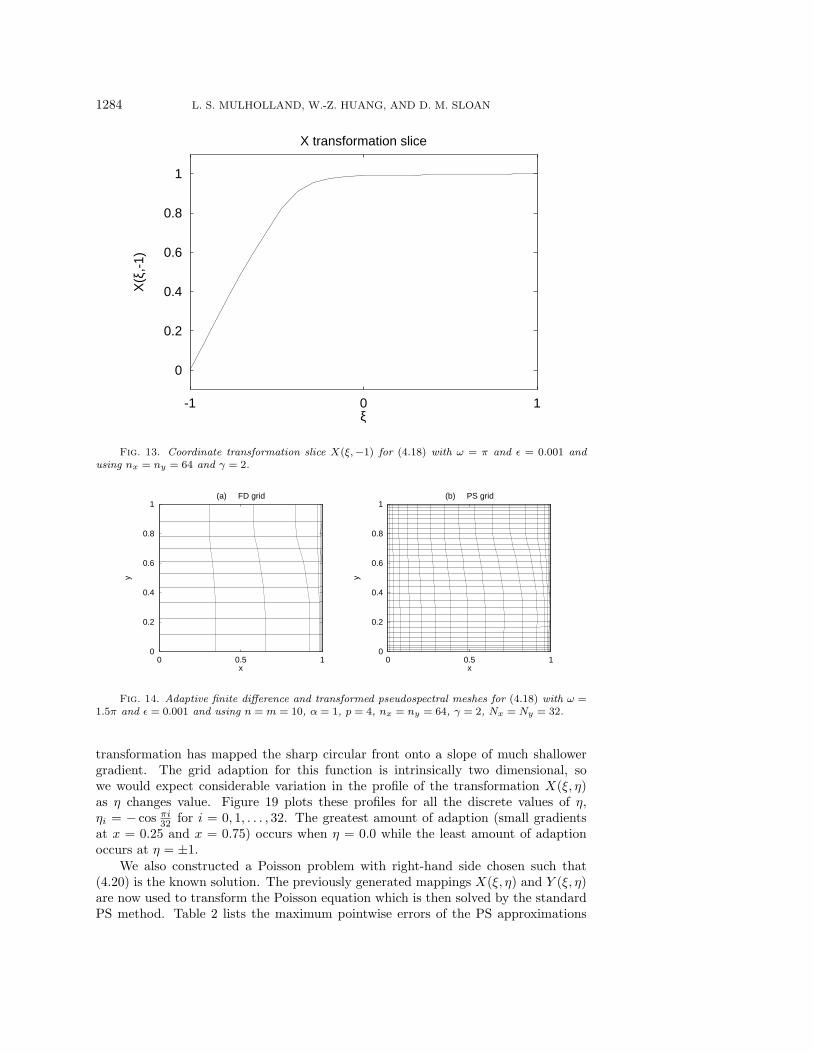
the grid will remain orthogonal. Figure 11 shows the adaptive finite difference andtransformed PS meshes generated for problem (4.18) with ω = π and ε = 0.001 andusing the parameter values listed in the caption. Figure 12 shows the correspondingadaptive transformation solution in both physical and computational coordinates; thissolution has a maximum pointwise error of 1.474× 10−4, whereas the adaptive finitedifference method has an error of 4.060 × 10−2. A cross section of the associatedtransformation X(ξ, η) for η = −1 is plotted in Figure 13—the cross section is verysimilar across all values of η; as expected the transformation Y (ξ, η) ≈ η ∀ξ.

0

0.2

0.4

0.6

0.8

1

0 0.5 1

y

x

(a) FD grid

0

0.2

0.4

0.6

0.8

1

0 0.5 1

y

x

(b) PS grid

Fig. 11. Adaptive finite difference and transformed PS meshes for (4.18) with ω = π andε = 0.001 and using n = m = 10, α = 1, p = 4, nx = ny = 64, γ = 2, Nx = Ny = 32.

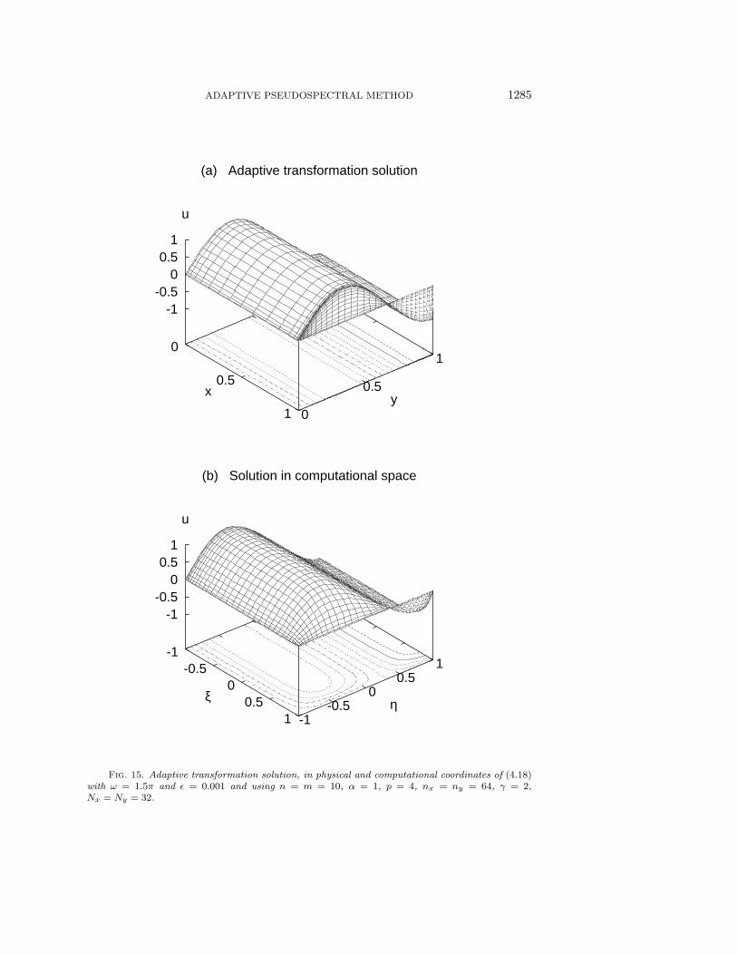
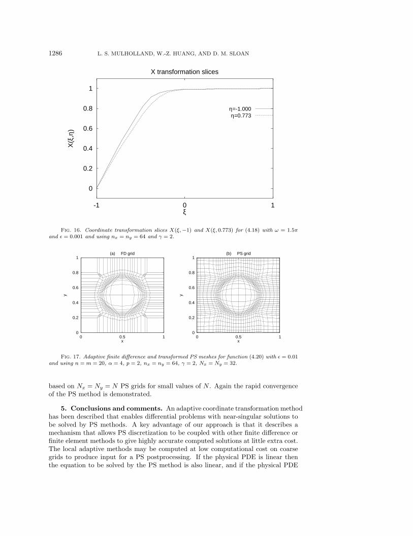
If we now set ω = 1.5π in (4.18) then we would expect a small amount of gridadaption in the y direction and some variation in cross section of X(ξ, η) for differ-ent values of η. Figure 14 shows the adaptive finite difference and transformed PSmeshes generated for problem (4.18) with ω = 1.5π and all other parameter valuesunaltered. Figure 15 shows the corresponding adaptive transformation solution inboth physical and computational coordinates; this solution has a maximum pointwiseerror of 1.105 × 10−3, whereas the adaptive finite difference method has an error of5.839× 10−2. Cross sections of the associated transformation X(ξ, η) for η = −1 andη = 0.773 are plotted in Figure 16—the cross sections do vary slightly with η.

Example 4.2. Fit a PS grid to

u = tanh

[1

ε

(1

16−(x− 1

2

)2

−(y − 1

2

)2)]

.(4.20)

For small ε this function resembles a top hat with front located on the circle(x− 1

2 )2+(y− 12 )2 = 1

16 . We use the adaptive finite difference method with n = m = 20,α = 4, and p = 2 to generate a finite difference grid for the function with ε = 0.01.The transformation method is then used, with settings nx = my = 64 and γ = 2,to generate mappings X(ξ, η) and Y (ξ, η) which allow u to be transformed into afunction of ξ and η. This done, an Nx = My = 32 PS grid is laid in (ξ, η) space.Figure 17 shows the finite difference and PS grids adapted to the function (4.20).Note that the finite difference grid actually crosses due to the high level of adaption(α = 4) and the low level of smoothing (p = 2), while the PS grid does not cross.This is a clear case of wrinkles in the initial data being smoothed out by the filteringprocess used in obtaining X(ξ, η) and Y (ξ, η). Figure 18 shows how the coordinate


(a) Adaptive transformation solution

0

0.5

1

x

0

0.5

1

y

0

0.5

1

u

(b) Solution in computational space

-1-0.5

00.5

1

ξ

-1-0.5

00.5

1

η

0

0.5

1

u

Fig. 12. Adaptive transformation solution, in physical and computational coordinates of (4.18)with ω = π and ε = 0.001 and using n = m = 10, α = 1, p = 4, nx = ny = 64, γ = 2, Nx = Ny = 32.


0

0.2

0.4

0.6

0.8

1

-1 0 1

X(ξ

,-1)

ξ

X transformation slice

Fig. 13. Coordinate transformation slice X(ξ,−1) for (4.18) with ω = π and ε = 0.001 andusing nx = ny = 64 and γ = 2.

0

0.2

0.4

0.6

0.8

1

0 0.5 1

y

x

(a) FD grid

0

0.2

0.4

0.6

0.8

1

0 0.5 1

y

x

(b) PS grid

Fig. 14. Adaptive finite difference and transformed pseudospectral meshes for (4.18) with ω =1.5π and ε = 0.001 and using n = m = 10, α = 1, p = 4, nx = ny = 64, γ = 2, Nx = Ny = 32.

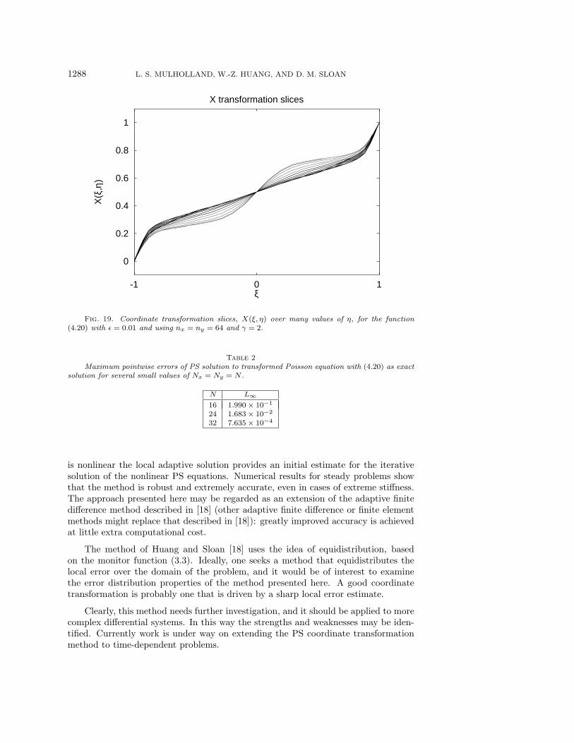
transformation has mapped the sharp circular front onto a slope of much shallowergradient. The grid adaption for this function is intrinsically two dimensional, sowe would expect considerable variation in the profile of the transformation X(ξ, η)as η changes value. Figure 19 plots these profiles for all the discrete values of η,ηi = − cos πi

32 for i = 0, 1, . . . , 32. The greatest amount of adaption (small gradientsat x = 0.25 and x = 0.75) occurs when η = 0.0 while the least amount of adaptionoccurs at η = ±1.

We also constructed a Poisson problem with right-hand side chosen such that(4.20) is the known solution. The previously generated mappings X(ξ, η) and Y (ξ, η)are now used to transform the Poisson equation which is then solved by the standardPS method. Table 2 lists the maximum pointwise errors of the PS approximations


(a) Adaptive transformation solution

0

0.5

1

x

0

0.5

1

y

-1-0.5

00.5

1

u

(b) Solution in computational space

-1-0.5

00.5

1

ξ

-1-0.5

00.5

1

η

-1-0.5

00.5

1

u

Fig. 15. Adaptive transformation solution, in physical and computational coordinates of (4.18)with ω = 1.5π and ε = 0.001 and using n = m = 10, α = 1, p = 4, nx = ny = 64, γ = 2,Nx = Ny = 32.


0

0.2

0.4

0.6

0.8

1

-1 0 1

X(ξ

,η)

ξ

X transformation slices

η=-1.000η=0.773

Fig. 16. Coordinate transformation slices X(ξ,−1) and X(ξ, 0.773) for (4.18) with ω = 1.5πand ε = 0.001 and using nx = ny = 64 and γ = 2.

0

0.2

0.4

0.6

0.8

1

0 0.5 1

y

x

(a) FD grid

0

0.2

0.4

0.6

0.8

1

0 0.5 1

y

x

(b) PS grid

Fig. 17. Adaptive finite difference and transformed PS meshes for function (4.20) with ε = 0.01and using n = m = 20, α = 4, p = 2, nx = ny = 64, γ = 2, Nx = Ny = 32.

based on Nx = Ny = N PS grids for small values of N . Again the rapid convergenceof the PS method is demonstrated.

5. Conclusions and comments. An adaptive coordinate transformation methodhas been described that enables differential problems with near-singular solutions tobe solved by PS methods. A key advantage of our approach is that it describes amechanism that allows PS discretization to be coupled with other finite difference orfinite element methods to give highly accurate computed solutions at little extra cost.The local adaptive methods may be computed at low computational cost on coarsegrids to produce input for a PS postprocessing. If the physical PDE is linear thenthe equation to be solved by the PS method is also linear, and if the physical PDE


(a) Function in physical space

00.2

0.40.6

0.81

x0

0.20.4

0.60.8

1

y

-1.5-1

-0.50

0.51

u

(b) Function in computational space

-1-0.5

00.5

1ξ

-1-0.5

00.5

1

η

-1.5-1

-0.50

0.51

u

Fig. 18. Function (4.20) with ε = 0.01 fitted to PS mesh in both physical and computationalcoordinates using n = m = 20, α = 4, p = 2, nx = ny = 64, γ = 2, Nx = Ny = 32.


0

0.2

0.4

0.6

0.8

1

-1 0 1

X(ξ

,η)

ξ

X transformation slices

Fig. 19. Coordinate transformation slices, X(ξ, η) over many values of η, for the function(4.20) with ε = 0.01 and using nx = ny = 64 and γ = 2.

Table 2Maximum pointwise errors of PS solution to transformed Poisson equation with (4.20) as exact

solution for several small values of Nx = Ny = N .

N L∞16 1.990× 10−1

24 1.683× 10−2

32 7.635× 10−4

is nonlinear the local adaptive solution provides an initial estimate for the iterativesolution of the nonlinear PS equations. Numerical results for steady problems showthat the method is robust and extremely accurate, even in cases of extreme stiffness.The approach presented here may be regarded as an extension of the adaptive finitedifference method described in [18] (other adaptive finite difference or finite elementmethods might replace that described in [18]): greatly improved accuracy is achievedat little extra computational cost.

The method of Huang and Sloan [18] uses the idea of equidistribution, basedon the monitor function (3.3). Ideally, one seeks a method that equidistributes thelocal error over the domain of the problem, and it would be of interest to examinethe error distribution properties of the method presented here. A good coordinatetransformation is probably one that is driven by a sharp local error estimate.

Clearly, this method needs further investigation, and it should be applied to morecomplex differential systems. In this way the strengths and weaknesses may be iden-tified. Currently work is under way on extending the PS coordinate transformationmethod to time-dependent problems.


REFERENCES

[1] J. M. Augenbaum, An adaptive pseudospectral method for discontinuous problems, Appl. Nu-mer. Math., 5 (1989), pp. 459–480.

[2] C. Basdevant, M. Deville, P. Haldenwang, J. M. Lacroix, D. Orlandi, A. Patera, R.Peyret, and J. Quazzani, Spectral and finite difference solutions of Burgers’ equation,Comput. Fluids, 14 (1986), pp. 23–41.

[3] A. Bayliss, D. Gottlieb, B. Matkowsky, and M. Minkoff, An adaptive pseudospectralmethod for reaction diffusion problems, J. Comput. Phys., 81 (1989), pp. 421–443.

[4] A. Bayliss and B. Matkowsky, Fronts, relaxation oscillations and period doubling in solidfuel combustion, J. Comput. Phys., 71 (1987), pp. 147–188.

[5] A. Bayliss and E. Turkel, Mappings and accuracy for Chebyshev pseudospectral approxima-tions, J. Comput. Phys., 101 (1992), pp. 349–359.

[6] J. U. Brackbill and J. S. Saltzman, Adaptive zoning for singular problems in two dimen-sions, J. Comput. Phys., 46 (1982), pp. 342–368.

[7] W. Cai, D. Gottlieb, and C.-W. Shu, Essentially nonoscillatory spectral Fourier methodsfor shock wave calculation, Math. Comput., 52 (1989), pp. 389–410.

[8] W. Cai, D. Gottlieb, and C.-W. Shu, On one-sided filters for spectral Fourier approximationof discontinuous functions, SIAM J. Numer. Anal., 29 (1992), pp. 905–916.

[9] C. Canuto, M. Y. Hussaini, A. Quarteroni, and T. A. Zang, Spectral Methods in FluidDynamics, Springer-Verlag, Berlin, Heidelberg, New York, 1988.

[10] E. A. Dorfi and L. O’C. Drury, Simple adaptive grids for 1-D initial value problems, J.Comput. Phys., 69 (1987), pp. 175–195.

[11] B. Fornberg and D. M. Sloan, A review of PS methods for solving PDEs, Acta Numerica,(1994), pp. 203–267.

[12] D. Gottlieb, L. Lustman, and S. A. Orszag, Spectral calculations in one-dimensional in-viscid compressible flow, SIAM J. Sci. Statist. Comput., 2 (1981), pp. 296–310.

[13] D. Gottlieb and S. A. Orszag, Numerical Analysis of Spectral Methods, SIAM, Philadelphia,1977.

[14] H. Guillard and R. Peyret, On the use of spectral methods for the numerical solution ofstiff problems, Comput. Meth. Appl. Mech. Engrg., 66 (1988), pp. 17–43.

[15] D. F. Hawken, J. J. Gottlieb, and J. S. Hansen, Review of some adaptive node-movementtechniques in finite element and finite difference solutions of PDEs, J. Comput. Phys., 95(1991), pp. 254–302.

[16] W.-Z. Huang and R. D. Russell, Analysis of Moving Mesh PDEs with Spatial Smoothing,Simon Fraser Mathematics Research Report, Simon Fraser University, Burnaby, BC, 1993,pp. 93–17.

[17] W.-Z. Huang and D. M. Sloan, A new pseudospectral method with upwind features, IMA J.Numer. Anal., 13 (1993), pp. 413–430.

[18] W.-Z. Huang and D. M. Sloan, A simple adaptive grid method in two dimensions, SIAM J.Sci. Comput., 15 (1994), pp. 776–797.

[19] D. Leviatan, Monotone and comonotone polynomial approximation revisited, J. Approx. The-ory, 53 (1988), pp. 1–16.

[20] J. A. Mackenzie, The efficient generation of simple two-dimensional adaptive grids, SIAM J.Sci. Comput., (1998), to appear.

[21] A. Majda, J. McDonough, and S. Osher, The Fourier method for non-smooth initial data,Math. Comput., 32 (1978), pp. 1041–1081.

[22] L. S. Mulholland and D. M. Sloan, The effect of filtering on the pseudospectral solution ofevolutionary partial differential equations, J. Comput. Phys., 96 (1991), pp. 369–390.

[23] E. Tadmor, Convergence of spectral methods for nonlinear conservation laws, SIAM J. Numer.Anal., 26 (1989), pp. 30–44.

[24] E. Tadmor, Shock capturing by the spectral viscosity method, Comput. Meth. Appl. Mech.Engrg., 80 (1990), pp. 197–208.

[25] E. Tadmor, Local error estimates for discontinuous solutions of nonlinear hyperbolic equations,SIAM J. Numer. Anal., 28 (1991), pp. 891–906.

[26] T. Tang and M. R. Trummer, Boundary layer resolving pseudospectral methods for singularperturbation problems, SIAM J. Sci. Comput., 17 (1996), pp. 430–438.

[27] J. F. Thompson, Z. U. A. Warsi, and C. W. Mastin, Numerical Grid Generation, North–Holland, New York, 1985.

[28] A. B. White, On selection of equidistribution meshes for two-point boundary value problems,SIAM J. Numer. Anal., 16 (1979), pp. 472–502.

Documents

PSEUDOSPECTRAL SOLUTION OF NEAR …people.ku.edu/~wzhuang/research/paper/MHS98.pdf · PSEUDOSPECTRAL SOLUTION OF NEAR-SINGULAR PROBLEMS USING NUMERICAL COORDINATE TRANSFORMATIONS