Provenance and data differencing for workﬂow

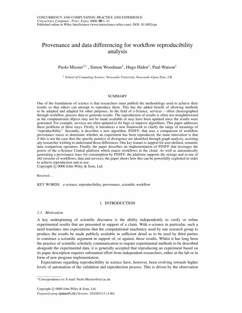
CONCURRENCY AND COMPUTATION: PRACTICE AND EXPERIENCEConcurrency Computat.: Pract. Exper. 0000; 00:1–21Published online in Wiley InterScience (www.interscience.wiley.com). DOI: 10.1002/cpe

Provenance and data differencing for workflow reproducibilityanalysis

Paolo Missier1∗ , Simon Woodman1, Hugo Hiden1, Paul Watson1

1 School of Computing Science, Newcastle University, Newcastle-Upon-Tyne, UK

SUMMARY

One of the foundations of science is that researchers must publish the methodology used to achieve theirresults so that others can attempt to reproduce them. This has the added benefit of allowing methodsto be adopted and adapted for other purposes. In the field of e-Science, services – often choreographedthrough workflow, process data to generate results. The reproduction of results is often not straightforwardas the computational objects may not be made available or may have been updated since the results weregenerated. For example, services are often updated to fix bugs or improve algorithms. This paper addressesthese problems in three ways. Firstly, it introduces a new framework to clarify the range of meanings of“reproducibility”. Secondly, it describes a new algorithm, PDIFF, that uses a comparison of workflowprovenance traces to determine whether an experiment has been reproduced; the main innovation is thatif this is not the case then the specific point(s) of divergence are identified through graph analysis, assistingany researcher wishing to understand those differences. One key feature is support for user-defined, semanticdata comparison operators. Finally, the paper describes an implementation of PDIFF that leverages thepower of the e-Science Central platform which enacts workflows in the cloud. As well as automaticallygenerating a provenance trace for consumption by PDIFF, the platform supports the storage and re-use ofold versions of workflows, data and services; the paper shows how this can be powerfully exploited in orderto achieve reproduction and re-use.Copyright c© 0000 John Wiley & Sons, Ltd.

Received . . .

KEY WORDS: e-science, reproducibility, provenance, scientific workflow

1. INTRODUCTION

1.1. Motivation

A key underpinning of scientific discourse is the ability independently to verify or refuteexperimental results that are presented in support of a claim. With e-science in particular, such aneed translates into expectations that the computational machinery used by one research group toproduce the results be made publicly available in sufficient detail as to be used by third partiesto construct a scientific argument in support of, or against, those results. Whilst it has long beenthe practice of scientific scholarly communication to require experimental methods to be describedalongside the experimental data, it is generally accepted that reproducing an experiment based onits paper description requires substantial effort from independent researchers, either in the lab or inform of new program implementation.

Expectations regarding reproducibility in science have, however, been evolving towards higherlevels of automation of the validation and reproduction process. This is driven by the observation

∗Correspondence to: E-mail: [email protected]

Copyright c© 0000 John Wiley & Sons, Ltd.Prepared using cpeauth.cls [Version: 2010/05/13 v3.00]

2 P. MISSIER, S. WOODMAN, H, HIDEN, P. WATSON

that actual acceleration of the production of scientific results, enabled by technology infrastructurewhich provides elastic computational facilities for “big data” e-science, is critically dependentupon the large-scale availability of datasets themselves, their sharing, and their use in collaborativesettings.

Following this observation, new social incentives are being tested with the goal of encouraging,and in some cases forcing, the publication of datasets associated with the results published inpapers. Evidence of increasing sharing can be found mostly in the form of online repositories. Theseinclude, amongst others, the recently created Thomson’s Data Citation Index†; the Dryad repositoryfor published data underlying articles in the biosciences (datadryad.org/); the databib.orgregistry of data repositories (databib.org/) (over 200 user contributed repository entries attime of writing), as well as Best Practice guidelines for data publication, issued by data preservationprojects like DataONE‡.

This dissemination phenomenon combines with the increasing rate at which publishable datasets are being produced, resulting in the need for automated validation and quality controlof the experimental methods and of their outcomes, all of which imposes new reproducibilityrequirements. Here the term reproducibility denotes the ability for a third party who has access tothe description of the original experiment and its results to reproduce those results using a possiblydifferent setting, with the goal to to confirm or dispute the original experimenter’s claims. Notethat this subsumes, and is hopefully more interesting, than the simpler case of repeatability, i.e.the attempt to replicate an experiment and obtain the same exact results when no changes occuranywhere.

In this paper we focus on the specific setting of workflow-based experiments, where reproductioninvolves creating a new version of the original experiment, while possibly altering some of theconditions (technical environment, scientific assumptions, input datasets). In this setting, we addressthe need to support experimenters in comparing results that may diverge because of those changes,and to help them diagnose the causes of such divergence. Depending on the technical infrastructureused to carry out the original experiment, different technical hurdles may stand in the way ofrepeatability and reproducibility. The apparently simple task of repeating a completely automatedprocess that was implemented for example using workflow technology, after a period of time sincethe experiment was originally carried out, may be complicated by the evolution of the technicalenvironment that supports the implementation, as well as by changes in the state of surroundingdatabases, and other factors that are not within the control of the experimenter. This well-knownphenomenon, known as “workflow decay”, is one indication that complete reproducibility maybe too ambitious even in the most favourable of settings, and that weaker forms of partialreproducibility should be investigated, as suggested by De Roure et al. [1]. Yet, it is easy to seethat this simple form of repeatability underpins the ability to reuse experiments designed by othersas part of new experiments. Cohen-Boulakia et al. elaborate on reusability specifically for workflow-based programming [2]: a older workflow that has ceased to function is not a candidate for reuse aspart of a new workflow that is being designed today.

Additional difficulties may be encountered when more computational infrastructure with specificdependencies (libraries, system configuration) is deployed to support data processing and analysis.For some of these, well-known techniques involving the use of virtual machines (VMs) can beused. VMs make complex applications self-contained by providing a runtime environment thatfulfills all of the applications dependencies. One can, for instance, create a VM containing anapplication consisting of a variety of bespoke scripts, along with all the libraries, databases andother dependencies that ensure the scripts can run successfully regardless of where the VMs aredeployed, including on public cloud nodes.

†wokinfo.com/products tools/multidisciplinary/dci/‡notebooks.dataone.org/bestpractices/

Copyright c© 0000 John Wiley & Sons, Ltd. Concurrency Computat.: Pract. Exper. (0000)Prepared using cpeauth.cls DOI: 10.1002/cpe

PROVENANCE AND DATA DIFFERENCING FOR REPRODUCIBILITY 3

1.2. Goals

VM technology is useful to provide a self-contained runtime environment, and indeed Groth etal. show that a combination of VM technology for partial workflow re-run along with provenancecan be useful in certain cases to promote reproducibility [3]. However, our contention is that itis the capability to compare execution traces and datasets with each other that sits at the coreof any argumentation that involves the reproduction of scientific results. Simple as it sounds, thisaspect of reproducibility seems to have received relatively little attention in the recent literature,with a few exceptions as noted later. Yet, without appropriate operational definitions of similarityof data, one cannot hope to answer the question of whether the outcome of an experiment is a validconfirmation of a previous version of the same, or of a similarly designed experiment. The workdescribed in this paper is focused primarily on this aspect of reproducibility, namely on addingdata-comparison capability to an existing e-science infrastructure, and to make it available to userscientists in addition to other reproducibility features, as a tool for supporting scientific discourse.

Our long term goal is to support experimenters in answering two related questions. Firstly, giventhe ability to carry out (variations of) the same experiments, to what extent can the outcomes of thoseexperiments be considered equivalent? Secondly, if they are not equivalent, what are the possiblecauses for the divergence?

Answering the first question is hard in general, as it requires knowledge of the type of the data,their format, and more importantly, their semantics. Consider for example two workflows, whichprocess data in a similar way but at some stage employ two different statistical learning techniquesto induce a classification model. Presumably, their outputs will be different for any execution ofeach of the two, and yet they may still be sufficiently close to be comparable. Thus, in this casea legitimate question is, are there suitable measures of data similarity that help support high-level conclusions of the form “the second method confirms the results of the first on a specificset of input datasets”? Answering this question requires knowledge of machine learning theory,namely to establish whether two classifiers can be considered equivalent, although the resultsthey produce are not identical. While the general problem of establishing data equivalence isknowledge-intensive, limiting the scope to simpler structural comparison may still lead to effectiveconclusions. For instance, for some applications that operate on XML data, it may be enoughto just define measures of similarity between two XML documents based on computing theirstructural differences, a problem successfully addressed by Wang et al. [4]. These examples suggesta spectrum of complexity in data similarity, starting from the simplest (two datasets are the sameif their files are byte-wise identical), to structurally more complex data structures (XML “diff”operators), to end with the harder problems of semantics-based similarity as in the earlier machinelearning example.

Our second question, regarding the diagnosis of the possible causes for dissimilarity of results,requires the ability to capture and then analyse the provenance traces associated with each of theexperiments. Stucturally, the provenance trace of a workflow execution is an acyclic digraph (DAG)in which the nodes denote either a piece of data or an activity, and the edges denote relationshipsamongst data and activities, which reflect the production and consumption of data throughout theworkflow execution steps (a simple but more formal definition is given in Sec. 2). While the problemof comparing two traces is in principle a classic one of finding subgraph isomorphisms in directedlabelled graphs [5, 6], greatly simplifying assumptions can be made by observing that workflowprovenance traces are a specific type of acyclic digraph with additional labelling, namely regardingthe ports on which activities produce and consume data items, which make it possible to reduce thespace of potential matches. Our assumption is that two provenance traces pertaining to two similarworkflows are expected to be structurally similar, and to contain data nodes that are comparable,in the sense clarified above. When this is the case, then there is hope that one can detect points inthe traces where results begin to diverge, and to diagnose the causes of such divergence by pairwisegraph traversal.



1.3. Contributions

We offer two main contributions, both set in the context of workflow-based e-science. Our referenceimplementation is based upon the e-Science Central workflow management system, developed byHiden et al. in our group [7]. The first contribution (Sec. 2) is a framework to characterise thereproducibility space, defined by the change in time of one or more of the technical elementsthat make up a computational experiment, leading to various forms of “workflow decay”, i.e.disfunctional or broken workflows.

The second contribution, described in Sec. 3, is PDIFF, an algorithm and prototypeimplementation to help users analyse diverging outputs that occur when trying to reproduceworkflows over time. This is complemented by an initial set of data comparison functions thataddress typical data types used in e-Science Central workflows. As these workflows are routinelyused to produce, for example, machine learning models for chemical engineering research [8], oursuite of data comparison functions includes the statistical similarity of predictive models producedusing machine learning techniques (in addition to comparing plain text files and XML documents).This set of functions is easily extensible, as they are implemented using workflow blocks, whichcan be rapidly implemented and deployed on the middleware.

Finally, in Sec. 4 we describe how PDIFF and the data diff functions leverage the currente-Science Central middleware and complement the functionality of its existing provenancemanagement sub-system. The technique described in the paper is not specific to the e-ScienceCentral platform, however. Indeed, since e-Science Central provenance is encoded using the OpenProvenance Model [9] (and will in the near future be aligned with the new PROV model [10]), itapplies to any provenance system that adopts the standard.

1.4. Related work

The perceived importance of enabling transparent, reproducible science has been growing overthe past few years. There is a misplaced belief, however, that adopting e-science infrastructuresfor computational science will automatically provide longevity to the programs that encode theexperimental methods. Evidence to the contrary, along with some analysis of the causes of non-reproducibility, is beginning to emerge, mainly in the form of editorials [11], [12]. The argument insupport of reproducible research, however, is not new, dating back from 2006 [13]. More recently,Dummond and Peng separately make a distinction between repeatability and reproducibility [14],[15]. Bechhofer et al. make a similar distinction concerning specifically the sharing of scientificdata [16].

In high profile Data Management conferences like SIGMOD, established initiatives to encouragecontributors to make their experiments reproducible and shareable have been ongoing for a numberof years, with some success§.

Technical solutions for ensuring reproducibility in computational sciences date back over 10years [17], but have matured more recently with workflow management systems (WFMS) likeGalaxy [18], [19] and VisTrails [20]. In both Galaxy and VisTrails, repeatability is facilitated byensuring that the evolution of the software components used in the workflows is controlled by theorganizations that design the workflows. This “controlled services” approach is shared by otherWFMS such as Kepler [21] and Knime (www.knime.org/), an open-source workflow-basedintegration platform for data analytics. This is in contrast to WFMS like Taverna [22], which are ableto orchestrate the invocation of operations over arbitrary web services, which makes it very generalbut also very vulnerable to version changes as well as maintenance issues of those services. A recentanalysis of the decay problem, conducted by Zhao et al. on about 100 Taverna workflows authoredbetween 2007 and 2012 that are published on the myExperiment repository, reveals that more than80% of those workflows either fail to produce the expected results, or fail to run altogether [23]. Sucha high failure rate is not surprising given that experimental workflows by their nature tend to makeuse, at least in part, of experimental services which are themselves subject to frequent changes or

§The SIGMOD reproducibility initiative: www.sigmod.org/2012/reproducibility.shtml.



may cease to be maintained. There are no obvious solutions to this problem, either, but the analysistechnique described in this paper applies to Taverna provenance traces [24], which comply withthe Open Provenance Model (and now with the W3C PROV model [10]). In this respect, e-ScienceCentral sits in the “closed world” camp, with versioned services data and workflows stored andmanaged by the platform. By default a workflow will make use of the latest version of a service, butthis can be overridden, to the extent that past versions are still available on the platform. In any case,the version history of each service can be queried, a useful feature for the application described inthis work.

The use of provenance to enable reproducibility has been explored in several settings. Moreaushowed that a provenance trace expressed using the Open Provenance Model can be given adenotation semantics (that is, an interpretation) that effectively amounts to “executing” a provenancegrpah and thus reproducing the computation it represents [25]. In the workflow setting, to the bestof our knowledge, VisTrails and Pegasus/Wings [26] are the only WFMS where the evolution ofworkflows is recorded, leading to a complete provenance trace that accounts for all edit operationsperformed by a designer to create a new version of an existing workflow, as shown by Koop etal. [27]. A similar feature is available in e-Science Central, namely in the form of a record historyof all versions of a workflow. Whilst edit scripts can potentially be constructed from such history,those are currently not explicit or in the form of a provenance trace. Thus, our divergence analysisis solely based upon the provenance of workflow executions, rather than the provenance of theworkflow itself. Note that this makes the technique more widely applicable, i.e. to the majority ofWFMS for which version history is not available.

Our technique falls under the general class of graph matching [28]. Specifically relevant is theheuristic polinomial algorithm for change detection in un-ordered trees, by Chawathe and Garcia-Molina [29]. Although matching provenance traces can be viewed as a change detection problem,it is less general because additional constraints on the data nodes, derived from the semantics ofprovenance graphs, reduce the space of possible matching candidates for any given node.

The idea of comparing workflow and provenance traces was explored by Altintas et al. [30] forthe Kepler system, with the goal of exploiting a database of traces as a cache to be used in lieuof repeating potentially expensive workflow computation wheneve possible. This “smart rerun”is based on matching provenance trace fragments with an upcoming computation fragment in aworkflow run, and replace the latter with the former when a match is found. This serves a differentpurpose from PDIFF, however. Whilst in SRM success is declared when a match is found, inPDIFF the interesting points in the graphs are those where divergence, rather than matching nodes,are detected.

Perhaps the most prominent research result on computing the difference of two provenance graphsis that of Bao et al. [31]. The premise of the work is that general workflow specifications that includearbitrary loops lead to provenance traces for which “differencing” is as complex as general subgraphisomorphism. The main insight is that the differencing problem becomes computationally feasibleunder the additional assumption that the workflow graphs have a series-parallel (s-p) structure,with well-nested forking and looping. While the e-Science Central workflow model does allowthe specification of non-s-p workflows, its loop facility is highly restricted, i.e. to a map operatorthat iterates over a list. Additionally, PDIFF relies on named input and output ports to steer thecoordinated traversal of two provenance graphs, as explained in Sec. 3.1. The combination of thesefeatures leads to a provenance comparison algorithm where each node is visited once.

2. A FRAMEWORK FOR REPRODUCIBILITY IN COMPUTATIONAL EXPERIMENTS

The framework presented in this section applies to generic computer programs for which provenancetraces can be generated. However, we restrict our attention to scientific workflows and workflowmanagement systems, as the approach described in the rest of the paper has been implementedspecifically for a workflow-based programming environment, namely eScience Central. Scientificworkflows and their virtues as a programming paradigm for the rapid prototyping of scienceapplications have been described at length by Deelman et al. [32]. For our purposes, we adopt



a minimal definition of workflow as a directed graph W = 〈T,E〉 consisting of a set T ofcomputational units (tasks) which are capable of producing and consuming data items on portsP and a set E ⊂ T × T of edges representing data dependencies amongst processors, such that〈ti.pA, tj .pB〉 ∈ E denotes that data produced by ti on port pA ∈ P is to be routed to port pB ∈ Pof task tj during the course of the computation¶. We write:

tr = exec(W,d,ED ,wfms) (1)

to denote the execution of a workflow W on input data d, with the additional indication that Wdepends on external elements such as third-party services and database state, collectively denotedED (for “External Dependencies”). W also depends on a runtime environment wfms , namely theworkflow management system.

The outcome of the execution is a graph-structured execution trace tr . A trace is defined by aset D of data items, a set A of activities, and a set R = {R1 . . . Rn} of relations Ri ⊂ (D ∪A)×(D ∪A). Different provenance models, including the OPM and PROV, introduce different typesof relations. For the purpose of this work, we adopt a simple model R = {used , genBy} whereused ⊂ A× P ×D and genBy ⊂ D ×A× P denote that an activity a has used data item d fromits port p, written used(a, p, d), and that d has been generated by a on port p, written genBy(d, a, p),respectively. Thus, a trace is simply a set of used and genBy records which are created duringone workflow run, from the observation of the inputs and outputs of each workflow block that isactivated. In particular, activities that appear in a trace correspond to instances, or invocations, oftasks that appear in the workflow. Distinguished data items in a trace for a workflow run are theinputs and the outputs of the workflow, denoted tr .I and tr .O respectively. Formally, tr .I = {d ∈D|a ∈ A ⇒ (d, a) /∈ genBy}. Symmetrically, tr .O = {d ∈ D|a ∈ A ⇒ (a, d) /∈ used}.

2.1. Evolution of workflow execution elements

At various points in time, each of the elements that participate in an execution may evolve, eitherindependently or in lock-step. This is represented by subscripting each of the elements in (1), asfollows:

tr t = exect(Wi,EDj , dh,wfmsk), with i, j, h, k < t (2)

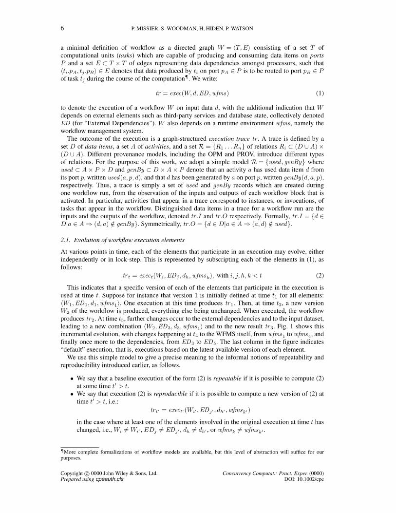
This indicates that a specific version of each of the elements that participate in the execution isused at time t. Suppose for instance that version 1 is initially defined at time t1 for all elements:〈W1,ED1, d1,wfms1〉. One execution at this time produces tr1. Then, at time t2, a new versionW2 of the workflow is produced, everything else being unchanged. When executed, the workflowproduces tr2. At time t3, further changes occur to the external dependencies and to the input dataset,leading to a new combination 〈W2,ED3, d3,wfms1〉 and to the new result tr3. Fig. 1 shows thisincremental evolution, with changes happening at t4 to the WFMS itself, from wfms1 to wfms4, andfinally once more to the dependencies, from ED3 to ED5. The last column in the figure indicates“default” execution, that is, executions based on the latest available version of each element.

We use this simple model to give a precise meaning to the informal notions of repeatability andreproducibility introduced earlier, as follows.

• We say that a baseline execution of the form (2) is repeatable if it is possible to compute (2)at some time t′ > t.

• We say that execution (2) is reproducible if it is possible to compute a new version of (2) attime t′ > t, i.e.:

tr t′ = exect′(Wi′ ,EDj′ , dh′ ,wfmsk′)

in the case where at least one of the elements involved in the original execution at time t haschanged, i.e., Wi 6= Wi′ , EDj 6= EDj′ , dh 6= dh′ , or wfmsk 6= wfmsk′ .

¶More complete formalizations of workflow models are available, but this level of abstraction will suffice for ourpurposes.



W ED d wfms

t1

t2

t3

W1

W2

ED1

ED3

d1

d3

wfms4t4

wfms1 tr1 = exec1(W1,SD1,d1,wfms1)

tr3 = exec3(W2,SD3,d3,wfms1)

tr5 = exec5(W2,SD5,d3,wfms4)ED5t5



Figure 1. Example of evolution timeline

Notice that a situation where data changes: dh → dh′ but Wi remains the same, or vice versa, mayrequire additional adapters to ensure that the new input can be used in the original workflow, or thatthe new workflow can accommodate the original input, respectively.

These simple definitions entail a number of issues that make repeating and reproducing executionscomplex in practice. Firstly, execution repetition becomes complicated when at least one theelements involved in the computation has changed between t and t′, because in this case each of theoriginal elements must have been saved and still made available. Secondly, reproducibility is nottrivial either, because in general there is no guarantee that the same workflow can be run with newexternal dependencies, or using a new version of the WFMS, or using a new input dataset.

Furthermore, we interpret the notion of reproducibility as a means by which experimentersvalidate results using deliberately altered conditions (Wi′ , dj′). In this case, the goal may not beto obtain exactly the original result, but rather one that is similar enough to it to conclude that theoriginal method and its results were indeed valid. Thus, we propose that reproducibility requires theability to compare the results tr t.O, tr t′ .O of two executions, using dedicated similarity functions,i.e., ∆D(tr t.O, tr t′ .O) (for example, one such function may simply detect whether the two datasetsare identical). However, a further complication arises as the criteria used to compare two data itemsin general depends on the type of the data, requiring the definition of a whole collection of ∆D

functions, one for each of possibly many data types of interest.A final problem arises when one concludes, after having computed exect(. . . ), exect′(. . . ), and

∆D(tr t.O, tr t′ .O), that the results are in fact not similar enough to conclude that the execution hasbeen successfully reproduced. In this case, one would like to identify the possible causes for suchdivergence.

We address these problems in the rest of the paper. In particular, after discussing generaltechniques for supporting repeatability and reproducibility, we focus on the last problem, namelythe role of provenance traces in diagnosing divergence in non-reproducible results, and describe aprototype implementation of such a diagnostic tool built as part of the eScience Central WFMS,underpinned by simple but representative data similarity functions.

2.2. Mapping the reproducibility space

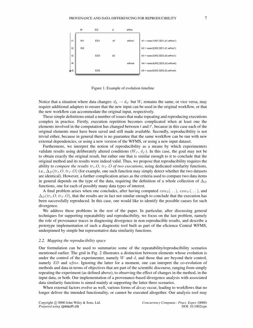
Our formulation can be used to summarize some of the repeatability/reproducibility scenariosmentioned earlier. The grid in Fig. 2 illustrates a distinction between elements whose evolution isunder the control of the experimenter, namely W and d, and those that are beyond their control,namely ED and wfms . Ignoring the latter for a moment, one can interpret the co-evolution ofmethods and data in terms of objectives that are part of the scientific discourse, ranging from simplyrepeating the experiment (as defined above), to observing the effect of changes in the method, in theinput data, or both. Our implementation of a provenance-based divergence analysis with associateddata similarity functions is aimed mainly at supporting the latter three scenarios.

When external factors evolve as well, various forms of decay occur, leading to workflows that nolonger deliver the intended functionality, or cannot be executed altogether. Our analysis tool may



dwf

dwf ! wf'

d ! d'wf

d ! d'wf ! wf'

ED

wfs wfs ! wfs'

ED ! ED'

resultsconfirmation

repeatability

reproducibility

Experimentalvariations

methodvariation

datavariation

data and method

variation

Environmental variations

decay region

disfunctionalworkflow

- service updates- state changes

non-functioningworkflow

exceptionanalysis,

debugging

divergenceanalysis

Figure 2. Mapping the reproducibility space

help diagnose the former case, where the results are not as expected and the cause is to be foundin new versions of third-party services, updated database states, or the non-deterministic behaviourof some of the workflow blocks. In contrast, exceptions analysis is required to diagnose a brokenworkflow, and it is out of the scope of this work.

3. PROVENANCE AND DATA DIFFERENCING

3.1. Detecting divergence in execution traces

In this section we present PDIFF, an algorithm designed to compare two provenance traces, tr t,tr t′ , that are generated from related executions, i.e., of the form (2) where at least one of the fourcontributing elements has changed between times t and t′. Specifically, the algorithm attempts toidentify differences in the two traces, which are due to one of the causes portrayed in Fig. 2, namelyworkflow evolution, input data evolution, as well as non-destructive external changes such as serviceand database state evolution. Note that we only consider cases where both executions succeed,although they may produce different results. We do not consider the cases of workflow decay thatlead to nonfunctional workflows, as those are best analysed using standard debugging techniques,and by looking at runtime exceptions.

The aim of the divergence detection algorithm is to identify whether two execution traces areidentical, and if they are not, where do they diverge. Specifically, given two outputs, one from eachof the two traces, the algorithm tries to match nodes from the two graphs by traversing them inlock-step as much as possible, from the bottom up, i.e., starting from the final workflow outputs.When mismatches are encountered, either because of differences in data content, or because ofnon-isomorphic graph structure, the algorithm records these mismatches in a “delta” data structureand then tries to continue by searching for new matching nodes further up in the traces. The deltastructure is a graph whose nodes are labelled with pairs of trace nodes that are expected to matchbut do not, as well as with entire fragments of trace graphs that break the continuity of the lock-steptraversal. Broadly speaking, the graph structure reflects the traversal order of the two graphs. A moredetailed account of the construction can be found in Sec. 3.2. Our goal is to compute a final deltatree that can be used to explain observed differences in workflow outputs, in terms of differencesthroughout the two executions. We first illustrate the idea in the case of simple data evolution:

tr t = exect(W,ED , d,wfms), tr t′ = exect′(W,ED , d′,wfms)



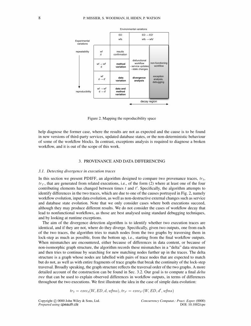
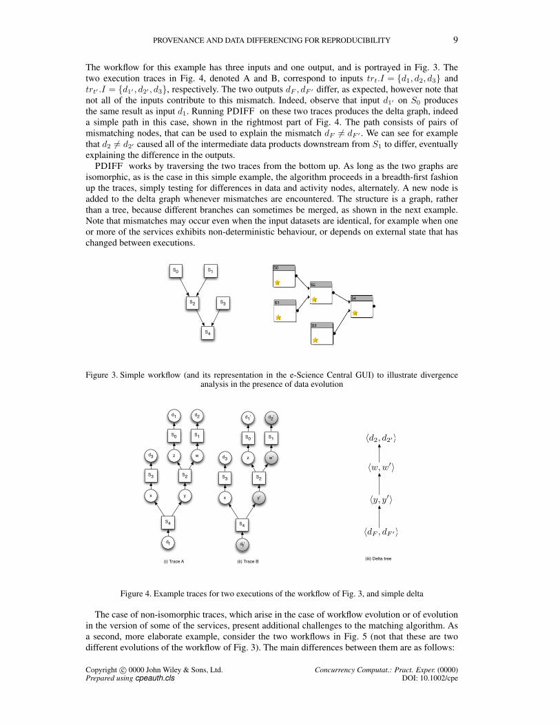
The workflow for this example has three inputs and one output, and is portrayed in Fig. 3. Thetwo execution traces in Fig. 4, denoted A and B, correspond to inputs trt.I = {d1, d2, d3} andtrt′ .I = {d1′ , d2′ , d3}, respectively. The two outputs dF , dF ′ differ, as expected, however note thatnot all of the inputs contribute to this mismatch. Indeed, observe that input d1′ on S0 producesthe same result as input d1. Running PDIFF on these two traces produces the delta graph, indeeda simple path in this case, shown in the rightmost part of Fig. 4. The path consists of pairs ofmismatching nodes, that can be used to explain the mismatch dF 6= dF ′ . We can see for examplethat d2 6= d2′ caused all of the intermediate data products downstream from S1 to differ, eventuallyexplaining the difference in the outputs.

PDIFF works by traversing the two traces from the bottom up. As long as the two graphs areisomorphic, as is the case in this simple example, the algorithm proceeds in a breadth-first fashionup the traces, simply testing for differences in data and activity nodes, alternately. A new node isadded to the delta graph whenever mismatches are encountered. The structure is a graph, ratherthan a tree, because different branches can sometimes be merged, as shown in the next example.Note that mismatches may occur even when the input datasets are identical, for example when oneor more of the services exhibits non-deterministic behaviour, or depends on external state that haschanged between executions.

S0 S1

S2 S3

S4

Figure 3. Simple workflow (and its representation in the e-Science Central GUI) to illustrate divergenceanalysis in the presence of data evolution

d1

S0

d2

S1

z w

S2

d3

yx

S3

S4

df

d1'

S0

d2'

S1

z w'

S2

d3

y'x

S3

S4

df'

(i) Trace A (ii) Trace B

�dF , dF ��

�y, y��

�w,w��

�d2, d2��

(iii) Delta tree

Figure 4. Example traces for two executions of the workflow of Fig. 3, and simple delta

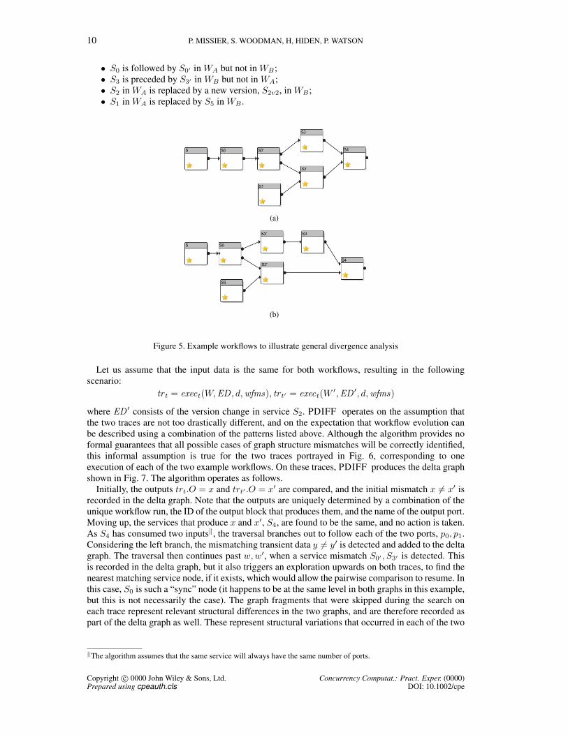
The case of non-isomorphic traces, which arise in the case of workflow evolution or of evolutionin the version of some of the services, present additional challenges to the matching algorithm. Asa second, more elaborate example, consider the two workflows in Fig. 5 (not that these are twodifferent evolutions of the workflow of Fig. 3). The main differences between them are as follows:



• S0 is followed by S0′ in WA but not in WB;• S3 is preceded by S3′ in WB but not in WA;• S2 in WA is replaced by a new version, S2v2, in WB;• S1 in WA is replaced by S5 in WB .

(a)

(b)

Figure 5. Example workflows to illustrate general divergence analysis

Let us assume that the input data is the same for both workflows, resulting in the followingscenario:

tr t = exect(W,ED , d,wfms), tr t′ = exect(W ′,ED ′, d,wfms)

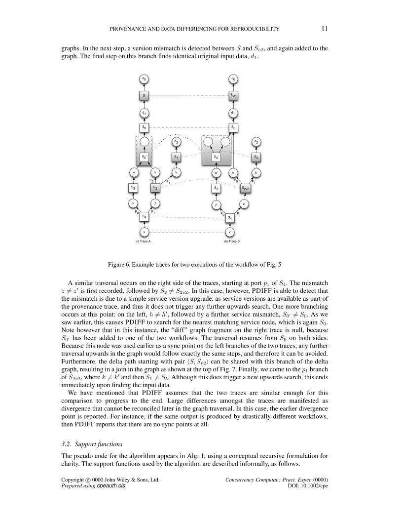
where ED ′ consists of the version change in service S2. PDIFF operates on the assumption thatthe two traces are not too drastically different, and on the expectation that workflow evolution canbe described using a combination of the patterns listed above. Although the algorithm provides noformal guarantees that all possible cases of graph structure mismatches will be correctly identified,this informal assumption is true for the two traces portrayed in Fig. 6, corresponding to oneexecution of each of the two example workflows. On these traces, PDIFF produces the delta graphshown in Fig. 7. The algorithm operates as follows.

Initially, the outputs trt.O = x and trt′ .O = x′ are compared, and the initial mismatch x 6= x′ isrecorded in the delta graph. Note that the outputs are uniquely determined by a combination of theunique workflow run, the ID of the output block that produces them, and the name of the output port.Moving up, the services that produce x and x′, S4, are found to be the same, and no action is taken.As S4 has consumed two inputs‖, the traversal branches out to follow each of the two ports, p0, p1.Considering the left branch, the mismatching transient data y 6= y′ is detected and added to the deltagraph. The traversal then continues past w,w′, when a service mismatch S0′ , S3′ is detected. Thisis recorded in the delta graph, but it also triggers an exploration upwards on both traces, to find thenearest matching service node, if it exists, which would allow the pairwise comparison to resume. Inthis case, S0 is such a “sync” node (it happens to be at the same level in both graphs in this example,but this is not necessarily the case). The graph fragments that were skipped during the search oneach trace represent relevant structural differences in the two graphs, and are therefore recorded aspart of the delta graph as well. These represent structural variations that occurred in each of the two

‖The algorithm assumes that the same service will always have the same number of ports.



graphs. In the next step, a version mismatch is detected between S and Sv2, and again added to thegraph. The final step on this branch finds identical original input data, d1.

d1

S0

S0'

w h

S3 S2

y z

S4

x

k

S1

d2

d1'

S0

k'h'

S3'

S2v2

w'

S3

S4

y' z'

x'

S5

d2

(i) Trace A (ii) Trace B

P0 P1P0 P1

P0 P0 P1P1

S Sv2

d0 d0

Figure 6. Example traces for two executions of the workflow of Fig. 5

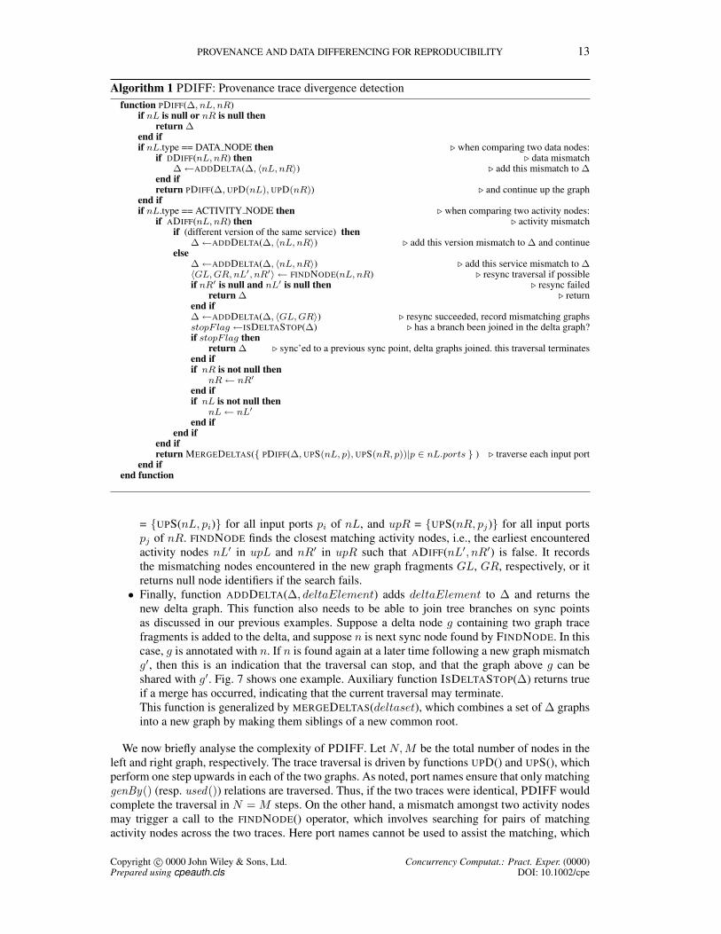
A similar traversal occurs on the right side of the traces, starting at port p1 of S4. The mismatchz 6= z′ is first recorded, followed by S2 6= S2v2. In this case, however, PDIFF is able to detect thatthe mismatch is due to a simple service version upgrade, as service versions are available as part ofthe provenance trace, and thus it does not trigger any further upwards search. One more branchingoccurs at this point: on the left, h 6= h′, followed by a further service mismatch, S0′ 6= S0. As wesaw earlier, this causes PDIFF to search for the nearest matching service node, which is again S0.Note however that in this instance, the “diff” graph fragment on the right trace is null, becauseS0′ has been added to one of the two workflows. The traversal resumes from S0 on both sides.Because this node was used earlier as a sync point on the left branches of the two traces, any furthertraversal upwards in the graph would follow exactly the same steps, and therefore it can be avoided.Furthermore, the delta path starting with pair 〈S, Sv2〉 can be shared with this branch of the deltagraph, resulting in a join in the graph as shown at the top of Fig. 7. Finally, we come to the p1 branchof S2v2, where k 6= k′ and then S1 6= S5. Although this does trigger a new upwards search, this endsimmediately upon finding the input data.

We have mentioned that PDIFF assumes that the two traces are similar enough for thiscomparison to progress to the end. Large differences amongst the traces are manifested asdivergence that cannot be reconciled later in the graph traversal. In this case, the earlier divergencepoint is reported. For instance, if the same output is produced by drastically different workflows,then PDIFF reports that there are no sync points at all.

3.2. Support functions

The pseudo code for the algorithm appears in Alg. 1, using a conceptual recursive formulation forclarity. The support functions used by the algorithm are described informally, as follows.



�x, x��

�y, y�� z, z��

�w,w��

�k, k��S0� , S3��

S0' S3'

�S1, S5�(service repl.)

�S2, S2v2�(version change)

�h, h��

S0'

P0 branch of S4 P1 branch of S4

P0 branch of S2 P1 branch of S2

�S,Sv2�(version change)

�d, d��

�S0, S0��

Figure 7. Delta graph from PDIFF on the traces of Fig. 6

• Functions UPD(d) and UPS(a, p) perform one step of the upwards graph traversal. Specifically,UPD(d) traverses a genBy(d, a) relation where d is a data node and returns the node for theactivity a that generated d. UPS(a, p) traverses a used(a, d, p) relation where a is an activitynode, and returns the node for the data d used by a through port p.

• Function DDIFF(nL, nR) defines datatype-specific comparison of data. This is used whenmatching the inputs and outputs of two workflow executions, i.e., tr t.I and tr t.O. Examplesof such data comparison functions are presented in the next section. Note that intermediateresults, represented as internal data nodes in the traces above, are transient data which are notexplicitly stored in the provenance database. To save space, only their MD-5 hash is recordedin the node. This results in a crude but very efficient data mismatch test for internal nodes withboolean result. In contrast, in the case of actual data the function may produce a similarityvalue between 0 and 1. For simplicity, we assume that a threshold is applied, so that datadiff functions all return TRUE if significant differences are detected, and FALSE otherwise∗∗.Similarly, function ADIFF(nL, nR) compares two service nodes using the service identifiers,and returns TRUE if the services are not the same. It can further flag differences that are duesolely to mismatches in service versions.

• FINDNODE(nL, nR) performs the search for a new matching node following a service nodemismatch. It returns a 4-tuple consisting of the graph fragments that were skipped duringthe search (either or both can be null), as well as references to the matching service nodesin each of the two traces, if they exist (note that either both of these are valid references,or neither is). More formally, consider the subgraphs upwards from nL and nR, i.e., upL

∗∗Whilst the transient nature of intermediate data does preclude the use of content-based comparison functions, note thatone can control the granularity of provenance, and thus the points where actual data is stored with it, by breaking downa complex workflow into a composition of smaller ones. Using small workflows is indeed typical for existing e-ScienceCentral applications.



Algorithm 1 PDIFF: Provenance trace divergence detectionfunction PDIFF(∆, nL, nR)

if nL is null or nR is null thenreturn ∆

end ifif nL.type == DATA NODE then . when comparing two data nodes:

if DDIFF(nL, nR) then . data mismatch∆←ADDDELTA(∆, 〈nL, nR〉) . add this mismatch to ∆

end ifreturn PDIFF(∆, UPD(nL), UPD(nR)) . and continue up the graph

end ifif nL.type == ACTIVITY NODE then . when comparing two activity nodes:

if ADIFF(nL, nR) then . activity mismatchif (different version of the same service) then

∆←ADDDELTA(∆, 〈nL, nR〉) . add this version mismatch to ∆ and continueelse

∆←ADDDELTA(∆, 〈nL, nR〉) . add this service mismatch to ∆〈GL, GR, nL′, nR′〉 ← FINDNODE(nL, nR) . resync traversal if possibleif nR′ is null and nL′ is null then . resync failed

return ∆ . returnend if∆←ADDDELTA(∆, 〈GL, GR〉) . resync succeeded, record mismatching graphsstopF lag ←ISDELTASTOP(∆) . has a branch been joined in the delta graph?if stopF lag then

return ∆ . sync’ed to a previous sync point, delta graphs joined. this traversal terminatesend ifif nR is not null then

nR← nR′

end ifif nL is not null then

nL← nL′

end ifend if

end ifreturn MERGEDELTAS({ PDIFF(∆, UPS(nL, p), UPS(nR, p))|p ∈ nL.ports } ) . traverse each input port

end ifend function

= {UPS(nL, pi)} for all input ports pi of nL, and upR = {UPS(nR, pj)} for all input portspj of nR. FINDNODE finds the closest matching activity nodes, i.e., the earliest encounteredactivity nodes nL′ in upL and nR′ in upR such that ADIFF(nL′, nR′) is false. It recordsthe mismatching nodes encountered in the new graph fragments GL, GR, respectively, or itreturns null node identifiers if the search fails.

• Finally, function ADDDELTA(∆, deltaElement) adds deltaElement to ∆ and returns thenew delta graph. This function also needs to be able to join tree branches on sync pointsas discussed in our previous examples. Suppose a delta node g containing two graph tracefragments is added to the delta, and suppose n is next sync node found by FINDNODE. In thiscase, g is annotated with n. If n is found again at a later time following a new graph mismatchg′, then this is an indication that the traversal can stop, and that the graph above g can beshared with g′. Fig. 7 shows one example. Auxiliary function ISDELTASTOP(∆) returns trueif a merge has occurred, indicating that the current traversal may terminate.This function is generalized by MERGEDELTAS(deltaset), which combines a set of ∆ graphsinto a new graph by making them siblings of a new common root.

We now briefly analyse the complexity of PDIFF. Let N,M be the total number of nodes in theleft and right graph, respectively. The trace traversal is driven by functions UPD() and UPS(), whichperform one step upwards in each of the two graphs. As noted, port names ensure that only matchinggenBy() (resp. used()) relations are traversed. Thus, if the two traces were identical, PDIFF wouldcomplete the traversal in N = M steps. On the other hand, a mismatch amongst two activity nodesmay trigger a call to the FINDNODE() operator, which involves searching for pairs of matchingactivity nodes across the two traces. Here port names cannot be used to assist the matching, which



therefore requires one activity node lookup in one of the graph, for each activity node in the othergraph. In the worst case, this results in N.M comparisons for a call to FINDNODE() that occurs nearthe bottom of the graph (i.e., at the first activity node from the bottom). As the traversal progressesupwards, more calls to FINDNODE() may occur, but they operate on progressively smaller fragmentsof the graphs, and any new search will stop at the first sync node that was found in a previous search(i.e., when function ISDELTASTOP() returns true). Considering the extreme cases, suppose thatdivergence is detected at the bottom of the graphs, and the only sync node is at the very top. Thisinvolves only one call to FINDNODE(), with cost approximately N.M , and then PDIFF terminates.In this case, the algorithm involves at most min(N,M) + N.M steps. The other extreme caseoccurs when the sync nodes are one step away from the diverging nodes. Now FINDNODE() iscalled repeatedly, at most min(N,M) times, but each time it completes after only one comparison,resulting in 2.min(N,M) steps.

To summarize, PDIFF is designed to assist reproducibility analysis by using provenance tracesfrom different executions to identify the following possible causes of diverging output values forthose executions:

• data and workflow evolution;• non-deterministic behaviour in some of the services, including the apparent non-determinism

due to changes in external service (or database) state;• service version upgrades.

3.3. Differencing data (DDiff)

Determining the similarity between two data sets is highly dependant not only on the type andrepresentation but also the semantics of the data. Not all data sets can be compared using a byte-wise comparator to determine if they are equivalent. For example, two models produced from thesame data set may well be equivalent but are unlikely to be byte-wise identical. In addition, aBoolean response of equivalent or not equivalent is a somewhat naıve approach and may providefalse negatives and be less amenable to statistical analysis.

Within e-Science Central we have built a flexible architecture in which it is possible toembed different algorithms for different types and representations of data. Following the standardextensibility model of e-Science Central, new data comparison functions can be implemented asworkflow blocks (typically as Java classes that interact with the system’s API).

We provide algorithms which calculate the equivalent of three classes of data. The algorithms areimplemented as e-Science Central workflows (described in Section 4) which implement a commoninterface allowing the system to determine dynamically which one to use for the relevant data set.

Text or CSV Comparing textual files is straightforward, and tools such as GNU diff or cmp††

are commonly used and well understood. By default GNU diff works by comparing eachfile, line by line, and returning the differences, known as hunks. It is possible to configurediff to ignore whitespace or text case differences which is useful for scientific data setswhere, for example, the header row may have different capitalisation but the data sets areotherwise identical. If no hunks are returned by diff the files are identical. However, if hunksare returned, the files differ in some way. In order to calculate the similarity, s, we return thepercentage of lines that are unchanged, converted to a number in the range 0 ≤ s ≤ 1

XML Comparing XML files is more complex than comparing textual data due to the semantic rulesgoverning its structure. For example, the ordering of attributes is not important, generally theorder of nodes is not important (although this is schema dependent) and where namespacesare used the prefix is not important. Existing work on comparing XML documents often triesto minimise the transformation necessary to turn one document into another (the so called,‘edit script’) or maximise the common structure from one document to another [33, 4, 34].

††gnu.org/software/diffutils/



For the purposes of comparing XML documents we use XOM (xom.nu/) which is ableto canonicalise XML documents so that they can be compared. Again, similarity, s is thepercentage of the document which has changed where 0 ≤ s ≤ 1.

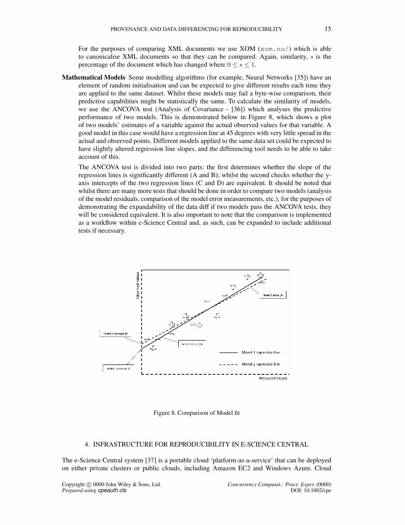
Mathematical Models Some modelling algorithms (for example, Neural Networks [35]) have anelement of random initialisation and can be expected to give different results each time theyare applied to the same dataset. Whilst these models may fail a byte-wise comparison, theirpredictive capabilities might be statistically the same. To calculate the similarity of models,we use the ANCOVA test (Analysis of Covariance - [36]) which analyses the predictiveperformance of two models. This is demonstrated below in Figure 8, which shows a plotof two models’ estimates of a variable against the actual observed values for that variable. Agood model in this case would have a regression line at 45 degrees with very little spread in theactual and observed points. Different models applied to the same data set could be expected tohave slightly altered regression line slopes, and the differencing tool needs to be able to takeaccount of this.

The ANCOVA test is divided into two parts: the first determines whether the slope of theregression lines is significantly different (A and B); whilst the second checks whether the y-axis intercepts of the two regression lines (C and D) are equivalent. It should be noted thatwhilst there are many more tests that should be done in order to compare two models (analysisof the model residuals, comparison of the model error measurements, etc.), for the purposes ofdemonstrating the expandability of the data diff if two models pass the ANCOVA tests, theywill be considered equivalent. It is also important to note that the comparison is implementedas a workflow within e-Science Central and, as such, can be expanded to include additionaltests if necessary.

Figure 8. Comparison of Model fit

4. INFRASTRUCTURE FOR REPRODUCIBILITY IN E-SCIENCE CENTRAL

The e-Science Central system [37] is a portable cloud ‘platform-as-a-service’ that can be deployedon either private clusters or public clouds, including Amazon EC2 and Windows Azure. Cloud



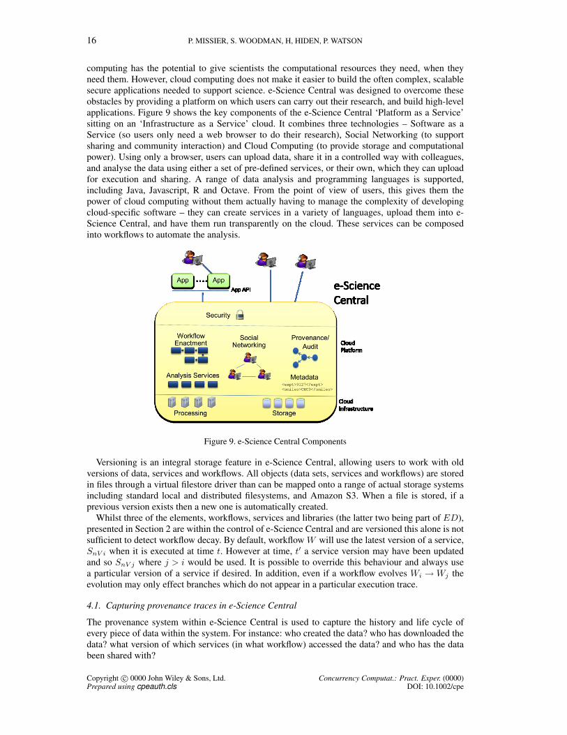
computing has the potential to give scientists the computational resources they need, when theyneed them. However, cloud computing does not make it easier to build the often complex, scalablesecure applications needed to support science. e-Science Central was designed to overcome theseobstacles by providing a platform on which users can carry out their research, and build high-levelapplications. Figure 9 shows the key components of the e-Science Central ‘Platform as a Service’sitting on an ‘Infrastructure as a Service’ cloud. It combines three technologies – Software as aService (so users only need a web browser to do their research), Social Networking (to supportsharing and community interaction) and Cloud Computing (to provide storage and computationalpower). Using only a browser, users can upload data, share it in a controlled way with colleagues,and analyse the data using either a set of pre-defined services, or their own, which they can uploadfor execution and sharing. A range of data analysis and programming languages is supported,including Java, Javascript, R and Octave. From the point of view of users, this gives them thepower of cloud computing without them actually having to manage the complexity of developingcloud-specific software – they can create services in a variety of languages, upload them into e-Science Central, and have them run transparently on the cloud. These services can be composedinto workflows to automate the analysis.

Figure 9. e-Science Central Components

Versioning is an integral storage feature in e-Science Central, allowing users to work with oldversions of data, services and workflows. All objects (data sets, services and workflows) are storedin files through a virtual filestore driver than can be mapped onto a range of actual storage systemsincluding standard local and distributed filesystems, and Amazon S3. When a file is stored, if aprevious version exists then a new one is automatically created.

Whilst three of the elements, workflows, services and libraries (the latter two being part of ED),presented in Section 2 are within the control of e-Science Central and are versioned this alone is notsufficient to detect workflow decay. By default, workflow W will use the latest version of a service,SnV i when it is executed at time t. However at time, t′ a service version may have been updatedand so SnV j where j > i would be used. It is possible to override this behaviour and always usea particular version of a service if desired. In addition, even if a workflow evolves Wi → Wj theevolution may only effect branches which do not appear in a particular execution trace.

4.1. Capturing provenance traces in e-Science Central

The provenance system within e-Science Central is used to capture the history and life cycle ofevery piece of data within the system. For instance: who created the data? who has downloaded thedata? what version of which services (in what workflow) accessed the data? and who has the databeen shared with?



Figure 10. e-Science Central Provenance Model

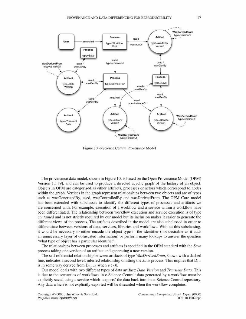
The provenance data model, shown in Figure 10, is based on the Open Provenance Model (OPM)Version 1.1 [9], and can be used to produce a directed acyclic graph of the history of an object.Objects in OPM are categorised as either artifacts, processes or actors which correspond to nodeswithin the graph. Vertices in the graph represent relationships between two objects and are of typessuch as wasGeneratedBy, used, wasControlledBy and wasDerivedFrom. The OPM Core modelhas been extended with subclasses to identify the different types of processes and artifacts weare concerned with. For example, execution of a workflow and a service within a workflow havebeen differentiated. The relationship between workflow execution and service execution is of typecontained and is not strictly required by our model but its inclusion makes it easier to generate thedifferent views of the process. The artifacts described in the model are also subclassed in order todifferentiate between versions of data, services, libraries and workflows. Without this subclassing,it would be necessary to either encode the object type in the identifier (not desirable as it addsan unnecessary layer of obfuscated information) or perform many lookups to answer the question‘what type of object has a particular identifier’.

The relationships between processes and artifacts is specified in the OPM standard with the Saveprocess taking one version of an artifact and generating a new version.

The self referential relationship between artifacts of type WasDerivedFrom, shown with a dashedline, indicates a second level, inferred relationship omitting the Save process. This implies that Di,v

is in some way derived from Di,v−1 when v > 0.Our model deals with two different types of data artifact: Data Version and Transient Data. This

is due to the semantics of workflows in e-Science Central: data generated by a workflow must beexplicitly saved using a service which ‘exports’ the data back into the e-Science Central repository.Any data which is not explicitly exported will be discarded when the workflow completes.



4.2. Provenance database implementation

Given that the provenance structure being stored is a directed acyclic graph, we chose to store itin the non-relational graph database, Neo4j (www.neo4j.org). Neo4j differs from traditionalrelational databases as its structure is not in terms of tables and rows and columns, but in nodes,relationships and properties. This provides a much more natural fit to our model, and allows us tostore the provenance graph directly instead of encoding it in a relational model. Neo4j has also beenshown to scale well, and most importantly, to perform well in terms of queries even when storing avery large graph structure [38]. Libraries are provided to allow users to work with Neo4j directly ineither Java or Ruby.

Various components within e-Science Central all log provenance information. From the outsetthe system was designed such that the order in which provenance events are received by the serveris not important. For instance, we could have an arbitrary interleaving of the events which signifythat a ‘Service has run’ and that the ‘Service accessed some data’. Each of these events contains asubset of information which must be added to the provenance database: the first event contains theservice name, start and completion time (and some other information) whereas the latter defines theidentity of the data which was read. Instead of SQL queries, Neo4j supports an operation known asa traversal whereby the user defines a starting node and rules about what types of relationship/nodeto ‘traverse’. The result is a set of paths from the starting node to the acceptable ending nodes. Theprovenance server is decoupled from e-Science Central with a durable JMS queue which allows e-Science Central to minimise the number of synchronous write operations which must be performedin a synchronous request.

4.3. Implementing PDIFF using Neo4j

The Neo4j database used by e-Science Central contains not just the execution traces which weare interested in traversing for PDIFF but also all the provenance for other items within e-ScienceCentral. For example, there may be multiple executions of each workflow but we are only interestedin two specific executions. Also, the provenance may indicate a data set may have been createdthrough a Save process which does not concern us.

The Neo4j traversal framework allows us to traverse the graph but restrict the traversal torelationships of a particular type and direction. During most of our traversals we restrict ourselvesto the used and genBy types with direction outgoing . This allows us to navigate back from theoutput data set in each execution trace back to the original input data sets. However, the semanticsof Neo4j traversals are that you are guaranteed to visit each node in the graph but not traverse everyedge. This would have the potential to miss branches in the execution trace which we should becomparing. To mitigate this we make additional calls to the database to ensure we retrieve all therelationships for each node.

As we traverse through the graph we build up a report containing the tree of ‘Delta’ descriptionsmaking use of the functions described below.

UPD(d) Navigates from either a Transient Data or Data Version node along an outgoing genByrelationship to the Service Run node which created it and returns this node. If there is no suchrelationship null is returned indicating the end of the graph. In this case, d is a Transient Datanode and an exception is thrown as this is an invalid starting point in the execution trace.

UPS(a, p) Navigates along an outgoing used relationship to a Transient Data or Data Version nodeand returns it. The Neo4j relationship which represents the edge contains an attribute for theport name p and so we filter based on this. If no such node is found an exception is thrown asthis is an invalid starting point to the execution trace.

DDIFF(NL, NR) If nL and nR are Transient Data nodes then this returns whether or not the MD-5hash values of the data are the same. If nL and nR are Data Version nodes then it will executeand e-Science Central workflow to determine whether or not the data sets are equivalent. Theworkflow executed is dependent on the MIME type of the data set as recorded as an attributeof the node in Neo4j.



ADIFF(NL, NR) This returns a 2-tuple containing whether or not the service identifier and versionidentifier for nL and nR are equal. In order to get the service and version identifier we mustnavigate the instanceOf relationship to the Service Version node in the provenance database.If either of the Service Version nodes is null then an exception is thrown as the graph is invalid.

FINDNODE(NL, NR) This performs a breadth first search of each of the execution traces in orderto try to find two nodes that enable the analysis to be re-synchronised. For brevity we willassume in the following discussion that the Service Run nodes can be compared directly –in practice we must navigate along the instanceOf relationship and perform the comparisonthere. Initially we select nL′ as a match candidate which is the next Service Run in the tracetraversing along used and genBy with direction outgoing . We then perform a breadth firsttraversal of the same relationship types beginning from nR searching for a match with nL′. Ifa match is found it is recorded as candidateL along with the depth at which it was found. Ifno match was found, we traverse back one step further from nL′ and repeat the search fromnR.If no candidate is found, the entire graph fragments from nL and nR are returned as there is nomatching node that enables the graphs to be re-synchronised. However, if a match is found, thesearch is re-performed but searching for nR′ nodes in the nL graph. When a second match isfound, namely candidateR, the search terminates. The returned nodes (and associated graphfragments) are those with the lowest combined depths from nL and nR. The second searchdeals with the case where a closer node match is found had we searched the other graph first.We can terminate on finding a match as we know that this will either be the same match asthe candidateL or a match with a lower combined depth. The nodes which are returned as asynchronisation point are also stored so that we are able to join future branches in the results.

ADDDELTA(∆, DATAELEMENT) Builds up the result graph. The results are constructed using asimple graph implementation where each node is able to contain one of the following objects:a Transient Data mismatch (the actual MD-5 hash values are of little use); the service andversion identifiers in case of a service or version change; or two graphs representing thegraph fragments which appear in one of the graphs but not the other. In the case of the graphfragments, the previous node nL and nR are included along with the subsequent nodes nL′

and nR′ for clarity. The result is stored in e-Science Central and can be exported to GraphMLfor visualisation or use in other applications.

At this time, the PDIFFimplementation is not yet integrated into e-Science Central. In the nextstage, the diagnosis functionality offered by the algorithm will be exposed to users through asimple interface. Users will be able to select two workflow runs and obtain a “diff” report on theirdivergence. Thanks to the relative small size of typical workflows, the diff graph can be visualizedas part of the e-Science Central web-based graphical interface.

5. CONCLUSIONS

The ability to reproduce experimental results underpins scientific discourse and is key to establishingcredibility in scholarly communication. Yet, several factors complicate the task of reproducing otherscientists’ results in settings other than the original one. Such factors include differences in theexperimental environment (different lab, research group, equipment technology) and insufficientdetail in the description of the methods. In computational science, the operating environmenttypically includes e-science infrastructure facilities, and the methods are formally encoded in theform of executable scripts, workflows, or general computer programs. This level of automationcreates the perception that the limitations in reproducibility of results can be easily overcome. Inreality, however, the traditional limiting factors are simply replaced by others, including an unstableand evolving operational environment, and lack of maintenance of related programs with mutualdependencies, which become unable to function together. As a result, scientific applications sufferfrom forms of decay that limit their longevity, and thus their reuse and evolution in time.



In this paper we have focused specifically on workflow-based e-science, and on a scenario whereattempts to reproduce earlier results translates into new runs of the same workflow at a later time.We assume that the workflow is still executable, but it may produce unexpected results or may havebeen made dysfunctional by changes in its system environment, or by uncontrolled evolution of theworkflow itself or of its input data.

We have presented two main contributions. Firstly, we have proposed a framework meant toclarify the range of meanings of the often ambiguous term “reproducibility”. We have then usedthe famework to situate our second contribution, namely the PDIFF algorithm for diagnosing thedivergence between two executions by comparing their associated provenance traces. We havealso described a number of data comparison function, which underpin provenance comparison.Finally, we have discussed the current implementation of PDIFF on the e-Science Central workflowmanagement middleware. PDIFF will be integrated in the public-facing version of e-ScienceCentral in the near future, with attention to usability testing, which has not being addressed inthe current prototype version.

REFERENCES

1. Roure DD, Belhajjame K, Missier P, Al E. Towards the preservation of scientific workflows. Procs. of the 8thInternational Conference on Preservation of Digital Objects (iPRES 2011), Singapore, 2011; 228–231.

2. Cohen-Boulakia S, Leser U. Search, adapt, and reuse: the future of scientific workflows. SIGMOD Rec.Sep 2011; 40(2):6–16, doi:http://doi.acm.org/10.1145/2034863.2034865. URL http://doi.acm.org/10.1145/2034863.2034865.

3. Groth P, Deelman E, Juve G, Mehta G, Berriman B. A Pipeline-Centric Provenance Model. The 4th Workshop onWorkflows in Support of Large-Scale Science, 2009.

4. Wang Y, DeWitt D, Cai JY. X-diff: an effective change detection algorithm for XML documents. Data Engineering,2003. Proceedings. 19th International Conference on, 2003; 519 – 530, doi:10.1109/ICDE.2003.1260818.

5. Berztiss AT. A Backtrack Procedure for Isomorphism of Directed Graphs. J. ACM Jul 1973; 20(3):365–377, doi:10.1145/321765.321766. URL http://doi.acm.org/10.1145/321765.321766.

6. Ullmann JR. An Algorithm for Subgraph Isomorphism. J. ACM Jan 1976; 23(1):31–42, doi:10.1145/321921.321925. URL http://doi.acm.org/10.1145/321921.321925.

7. Hiden H, Watson P, Woodman S, Leahy D. e-Science Central: Cloud-based e-Science and its application to chemicalproperty modelling. Technical report cs-tr-1227, School of Computing Science, Newcastle University 2011.

8. Cala J, Watson P, Woodman S. Cloud Computing for Fast Prediction of Chemical Activity. Procs. 2nd InternationalWorkshop on Cloud Computing and Scientific Applications (CCSA), Ottawa, Canada, 2012.

9. Moreau L, Clifford B, Freire J, Futrelle J, Gil Y, Groth P, Kwasnikowska N, Miles S, Missier P, Myers J, et al.. TheOpen Provenance Model — Core Specification (v1.1). Future Generation Computer Systems 2011; 7(21):743–756,doi:http://dx.doi.org/10.1016/j.future.2010.07.005.

10. Moreau L, Missier P, Belhajjame K, B’Far R, Cheney J, Coppens S, Cresswell S, Gil Y, Groth P, Klyne G,et al.. PROV-DM: The PROV Data Model. Technical Report, World Wide Web Consortium 2012. URL http://www.w3.org/TR/prov-dm/.

11. Hanson B, Sugden A, Alberts B. Making Data Maximally Available. Science 2011; 331(6018):649, doi:10.1126/science.1203354.

12. Merall Z. Computational science: ...Error. Nature Oct 2010; 467:775–777, doi:10.1038/467775a.13. Peng RD, Dominici F, Zeger SL. Reproducible Epidemiologic Research. American Journal of Epidemiology 2006;

163(9):783–789, doi:10.1093/aje/kwj093. URL http://aje.oxfordjournals.org/content/163/9/783.abstract.

14. Drummond C. Science, Replicability is not Reproducibility: Nor is it Good Science. Procs. 4th workshop onEvaluation Methods for Machine Learning In conjunction with ICML 2009, Montreal, Canada, 2009. URLhttp://cogprints.org/7691/7/ICMLws09.pdf.

15. Peng R. Reproducible Research in Computational Science. Science Dec 2011; 334(6060):1226–1127.16. Bechhofer S, De Roure D, Gamble M, Goble C, Buchan I. Research Objects: Towards Exchange and Reuse of

Digital Knowledge. Nature Precedings 2010; URL http://dx.doi.org/10.1038/npre.2010.4626.1.17. Schwab M, Karrenbach M, Claerbout J. Making Scientific Computations Reproducible. Computing in

Science Engineering 2000; 2(6):61–67, doi:10.1109/5992.881708. URL http://ieeexplore.ieee.org/lpdocs/epic03/wrapper.htm?arnumber=881708.

18. Mesirov J. Accessible Reproducible Research. Science 2010; 327. URL www.sciencemag.org.19. Nekrutenko A. Galaxy: a comprehensive approach for supporting accessible, reproducible, and transparent

computational research in the life sciences. Genome Biology 2010; 11(8):R86. URL http://dx.doi.org/10.1186/gb-2010-11-8-r86.

20. Scheidegger C, Vo H, Koop D, Freire J. Querying and Re-Using Workflows with VisTrails. Procs. SIGMOD, 2008;1251–1254. URL http://portal.acm.org/citation.cfm?id=1376747.

21. Ludascher B, Altintas I, Berkley C. Scientific Workflow Management and the Kepler System. Concurrency andComputation: Practice and Experience 2005; 18:1039–1065. URL http://onlinelibrary.wiley.com/doi/10.1002/cpe.994/abstract;jsessionid=B39961C2FDAF407AB30BCB118612D171.d02t02.



22. Missier P, Soiland-Reyes S, Owen S, Tan W, Nenadic A, Dunlop I, Williams A, Oinn T, Goble C. Taverna,reloaded. Procs. SSDBM 2010, Gertz M, Hey T, Ludaescher B (eds.), Heidelberg, Germany, 2010. URL http://www.ssdbm2010.org/.

23. Zhao J, Gomez-Perez J, Belhajjame K, Klyne G, Al E. Why Workflows Break - Understanding and CombatingDecay in Taverna Workflows. Procs. e-science conference, Chicago, 2012.

24. Missier P, Paton N, Belhajjame K. Fine-grained and efficient lineage querying of collection-based workflowprovenance. Procs. EDBT, Lausanne, Switzerland, 2010.

25. Moreau L. Provenance-based reproducibility in the Semantic Web. Web Semantics: Science, Services andAgents on the World Wide Web 2011; 9(2):202–221, doi:10.1016/j.websem.2011.03.001. URL http://www.sciencedirect.com/science/article/pii/S1570826811000163.

26. Kim J, Deelman E, Gil Y, Mehta G, Ratnakar V. Provenance trails in the Wings-Pegasus system. Concurrency andComputation: Practice and Experience 2008; 20:587–597, doi:http://dx.doi.org/10.1002/cpe.1228. URL http://www3.interscience.wiley.com/journal/115805532/abstract.

27. Koop D, Scheidegger C, Freire J, Silva C. The Provenance of Workflow Upgrades. Provenance and Annotation ofData and Processes, Lecture Notes in Computer Science, vol. 6378, McGuinness D, Michaelis J, Moreau L (eds.).Springer Berlin / Heidelberg, 2010; 2–16. URL http://dx.doi.org/10.1007/978-3-642-17819-1\2.

28. Bunke H. Graph Matching: Theoretical Foundations, Algorithms, and Applications. Procs. Vision Interface, 2000.29. Chawathe SS, Garcia-Molina H. Meaningful change detection in structured data. SIGMOD Rec. Jun 1997;

26(2):26–37, doi:10.1145/253262.253266. URL http://doi.acm.org/10.1145/253262.253266.30. Altintas I, Barney O, Jaeger-Frank E. Provenance Collection Support in the {K}epler Scientific Workflow System.

IPAW, 2006; 118–132, doi:http://dx.doi.org/10.1007/11890850\ 14.31. Bao Z, Cohen-Boulakia S, Davidson S, Eyal A, Khanna S. Differencing Provenance in Scientific Workflows.

Procs. ICDE, 2009, doi:http://dx.doi.org/10.1109/ICDE.2009.103. URL http://ieeexplore.ieee.org/xpl/freeabs\ all.jsp?tp=\&arnumber=4812456\&isnumber=4812372.

32. Deelman E, Gannon D, Shields M, Taylor I. Workflows and e-Science: An overview of workflow systemfeatures and capabilities. Future Generation Computer Systems 2009; 25(5):528–540, doi:DOI:10.1016/j.future.2008.06.012. URL http://www.sciencedirect.com/science/article/B6V06-4SYCPKX-2/2/bb631979e3dd7071ddede90bbff65a91.

33. Schubert E, Schaffert S, Bry F. Structure-preserving difference search for XML documents. Extreme MarkupLanguages R©, 2005.

34. Cobena G, Abiteboul S, Marian A. Detecting changes in XML documents. Data Engineering, 2002. Proceedings.18th International Conference on, 2002; 41 –52, doi:10.1109/ICDE.2002.994696.

35. Cybenko G. Approximation by superpositions of a sigmoidal function. Mathematics of Control, Sig-nals, and Systems (MCSS) 1989; 2:303–314. URL http://dx.doi.org/10.1007/BF02551274,10.1007/BF02551274.

36. Rutherford A. Introducing ANOVA and ANCOVA : a GLM approach. SAGE, 2001. URL http://www.worldcat.org/isbn/9780761951605.

37. Watson P, Hiden H, Woodman S. e-Science Central for CARMEN: science as a service. Concurrency andComputation: Practice and Experience December 2010; 22:2369–2380, doi:http://dx.doi.org/10.1002/cpe.v22:17.URL http://dx.doi.org/10.1002/cpe.v22:17.

38. Dominguez-Sal D, Urbon-Bayes P, Gimenez-Vano A, Gomez-Villamor S, Martınez-Bazan N, Larriba-Pey JL.Survey of graph database performance on the HPC scalable graph analysis benchmark. Proceedings of the 2010international conference on Web-age information management, WAIM’10, Springer-Verlag: Berlin, Heidelberg,2010; 37–48. URL http://dl.acm.org/citation.cfm?id=1927585.1927590.


Documents

Provenance and data differencing for workﬂow