Embed Size (px)
Citation preview

UNIVERSITE LIBRE DE BRUXELLES
Faculte des Sciences
Departement d’Informatique
Provably Correct Code Generation of
Real-Time Controllers
Memoire presente en vue de l’obtention
du grade de Licencie en Informatique
Nicolas MAQUET
Annee academique 2005–2006
Remerciements
Ce sujet de memoire m’a ete propose par M. Jean-Francois Raskin. Je tiens a leremercier pour son aide apportee tout au long de la realisation de ce travail. Sonenthousiasme pour la recherche et son intransigeance technique sont pour moides exemples.
Je tiens egalement a remercier M. Laurent Doyen et M. Martin De Wulf,et tout particulierement ce dernier pour avoir relu et commente de nombreusesversions de ce travail, et pour avoir repondu avec bonne humeur a mes myriadesde questions.
Je remercie tout le corps academique du Departement d’Informatique, pourleur travail de tous les jours a la realisation d’un enseignement scientifique dequalite.
Un grand merci a tous mes amis, pour leur chaleureux soutien dans les mo-ments difficiles et leur presence de tous les jours. Un remerciement tout par-ticulier a Thierri de Vos pour son interet enthousiaste a mes travaux, et pouravoir accepte de m’aider a la realisation d’un chapitre de ce memoire mais quin’a malheureusement pas abouti (il s’agissait d’une etude de cas supplementaireimpliquant des automates hybrides). Ton travail ne restera pas vain, ce n’est quepartie remise !
Enfin, je tiens a temoigner ma gratitude envers toute ma famille pour leuramour et leur soutien tout au long de mes etudes. Je ne peux pas vous remerciertous personnellement ici, mais je ne peux m’empecher de citer ceux et celles queje vois et qui me soutiennent quotidiennement (et qui donc, en particulier, ont dume supporter jour apres jour pendant la redaction de cet ouvrage . . . ) : Maman,Chloe, Roland, Martine, Maxime, Philippe, Catherine, Etienne, et Amandine.Merci !
ii

A mon frere, Laurent MaquetA mon pere, Philippe Maquet
iii

Contents
1 Introduction 21.1 Formal Methods for Software Verification . . . . . . . . . . . . . . 2
1.1.1 Bottom-Up Approach . . . . . . . . . . . . . . . . . . . . . 21.1.2 Top-Down Approach . . . . . . . . . . . . . . . . . . . . . 3
1.2 Provably Correct Real-Time Controllers . . . . . . . . . . . . . . 31.3 Modeling Real-Time Controllers with Timed Automata . . . . . . 41.4 Modeling Environments With Timed or
Hybrid Automata . . . . . . . . . . . . . . . . . . . . . . . . . . . 51.5 Synchrony Hypothesis . . . . . . . . . . . . . . . . . . . . . . . . 61.6 Syntax and Semantics . . . . . . . . . . . . . . . . . . . . . . . . 71.7 AASAP Semantics and Implementability . . . . . . . . . . . . . . 81.8 Implementing Controllers Systematically . . . . . . . . . . . . . . 81.9 Goal and Structure of this Work . . . . . . . . . . . . . . . . . . . 9
2 Timed Automata 112.1 Syntax of Timed Automata . . . . . . . . . . . . . . . . . . . . . 112.2 Classical Semantics of Timed Automata . . . . . . . . . . . . . . 152.3 Timed Systems Analysis . . . . . . . . . . . . . . . . . . . . . . . 192.4 Timed Automata in the Literature . . . . . . . . . . . . . . . . . 21
3 Implementability of Timed Controllers 223.1 Overview of the Almost ASAP Approach . . . . . . . . . . . . . . 243.2 Simulation and Controller Refinement . . . . . . . . . . . . . . . . 243.3 Elastic Controllers and ASAP Semantics . . . . . . . . . . . . . 263.4 Almost ASAP Semantics . . . . . . . . . . . . . . . . . . . . . . . 263.5 Almost ASAP Semantics Analysis . . . . . . . . . . . . . . . . . . 32
4 Implementation Semantics 334.1 Program Semantics . . . . . . . . . . . . . . . . . . . . . . . . . . 34
4.1.1 Formalization of the Program Semantics . . . . . . . . . . 354.1.2 Comments on the Program Semantics . . . . . . . . . . . . 364.1.3 AASAP Simulability of the Program Semantics . . . . . . 374.1.4 Implementability of the Program Semantics . . . . . . . . 38
iv

4.1.5 Limitations of the Program Semantics . . . . . . . . . . . 384.2 Real-Time Semantics . . . . . . . . . . . . . . . . . . . . . . . . . 40
4.2.1 Overview of the Real-Time Semantics . . . . . . . . . . . . 414.2.2 Formalization of the Real-Time Semantics . . . . . . . . . 424.2.3 AASAP Simulability of the Real-Time Semantics . . . . . 444.2.4 Implementability of the Real-Time Semantics . . . . . . . 514.2.5 Benefits of the Real-Time Semantics . . . . . . . . . . . . 52
5 RTAI : GNU/Linux Made RT Capable 535.1 Architecture of RTAI . . . . . . . . . . . . . . . . . . . . . . . . . 535.2 RTAI Service Routines . . . . . . . . . . . . . . . . . . . . . . . . 54
5.2.1 Timer Routines . . . . . . . . . . . . . . . . . . . . . . . . 545.2.2 Task-Management Routines . . . . . . . . . . . . . . . . . 56
5.3 The RTAI Scheduler . . . . . . . . . . . . . . . . . . . . . . . . . 57
6 Code Generation of Real-Time Controllers 596.1 Input Language . . . . . . . . . . . . . . . . . . . . . . . . . . . . 59
6.1.1 Specification Section . . . . . . . . . . . . . . . . . . . . . 596.1.2 Decoration Section . . . . . . . . . . . . . . . . . . . . . . 61
6.2 Code Generation . . . . . . . . . . . . . . . . . . . . . . . . . . . 666.2.1 Architecture of the Generated Code . . . . . . . . . . . . . 666.2.2 Correctness of the Generated Code . . . . . . . . . . . . . 72
6.3 Use of the Spectre Decoration Language . . . . . . . . . . . . . 736.4 Implementation of Spectre . . . . . . . . . . . . . . . . . . . . . 74
7 Case Study : Philips Audio Control Protocol 757.1 Description of the PACP . . . . . . . . . . . . . . . . . . . . . . . 767.2 Modeling the PACP with Timed Automata . . . . . . . . . . . . . 76
7.2.1 Sender Automaton . . . . . . . . . . . . . . . . . . . . . . 777.2.2 Receiver Automaton . . . . . . . . . . . . . . . . . . . . . 78
7.3 Verification Results . . . . . . . . . . . . . . . . . . . . . . . . . . 797.4 Systematic Implementation of the PACP
using Spectre . . . . . . . . . . . . . . . . . . . . . . . . . . . . 807.4.1 Sender Specification . . . . . . . . . . . . . . . . . . . . . 807.4.2 Sender Decoration . . . . . . . . . . . . . . . . . . . . . . 807.4.3 Receiver Specification . . . . . . . . . . . . . . . . . . . . . 827.4.4 Receiver Decoration . . . . . . . . . . . . . . . . . . . . . 827.4.5 Assigning the RT Semantics Parameters . . . . . . . . . . 84
7.5 Execution of the Generated Code . . . . . . . . . . . . . . . . . . 84
8 Conclusions 89
v

1
A Spectre Grammar 91A.1 Typographical Conventions Used . . . . . . . . . . . . . . . . . . 91A.2 Grammar . . . . . . . . . . . . . . . . . . . . . . . . . . . . . . . 91
B Example of Spectre Output 95
Chapter 1
Introduction
This work studies a methodology for creating provably correct real-time softwarecontrollers. A real-time software is a program for which the correctness dependsnot only on the soundness of its outputs, but also on the time at which thoseoutputs are produced. For instance, a nuclear power-plant emergency shutdownsequence might involve numerous steps such as opening valves, raising roboticarms, triggering sound alerts, etc. Each of those steps must be accomplished ina timely fashion in order to prevent a catastrophe. When the possible damagecaused by software failure reaches a certain point, it is more and more considerednecessary to have some kind of formal assurance that the control software willalways operate as required, that is by keeping the controlled environment in asafe state (the plant has not exploded, the aircraft has not crashed, etc.). Toobtain this formal assurance, we need a way of reasoning on control software suchthat a proof of correctness can be constructed. This is done by (1) constructinga formal model M of the system (including environment and control software),(2) by specifying a formal property ψ that the model needs to satisfy, and (3)by proving that M |= ψ. When such a proof can be obtained, we say that thecontrol software is provably correct.
1.1 Formal Methods for Software Verification
Several formal methods for creating provably correct software have been studiedin computer science, each having their own particularities. These methods canbe classified in two distinct categories, which we introduce in turn.
1.1.1 Bottom-Up Approach
One way of reasoning about software that yields correctness proofs works byproceeding bottom-up. Based on informal specifications, a software solution iscreated, using standard software design techniques. After this first step, the
2

CHAPTER 1. INTRODUCTION 3
control software and its environment are then abstracted, to provide a formalmodel. Great care has to be put into this abstraction phase, to make sure thatthe model is a sound over-approximation of the real system.
The notion of over-approximation is a key concept in software verification. Inshort, a formal model correctly over-approximates a real-world system if we havethat every property which can be proven true on the model will also be true forthe real system. This is done by ensuring that every possible behavior of the realsystem is included in the set of behaviors that the model contains. The modelcan contain more behaviors however, hence the term over-approximation.
Once the formal model has been created, it is possible to reason on that modelin a formal way, in order to obtain formal assurance that the real system is indeedcorrect (i.e. it satisfies some formal specification).
1.1.2 Top-Down Approach
Another approach to software verification (and the one we will use in this study)works the other way around. Using the informal specifications of the systemto implement, a model is created before the beginning of the implementationprocess. The same care has to be put into the model design than in the formerapproach, in order to reason on a sound over-approximation of the target system.This approach however, has one considerable advantage : after having verifiedthat the model is correct, it is possible to construct the implementation of thesoftware in a systematic way. This of course requires that the model be designedin such a way that a systematic implementation is possible. Another considerableadvantage of the top-down approach is that it can detect design flaws before theimplementation process. If severe errors are found after the implementation hasbeen created, part of the programming effort will have been wasted.
1.2 Provably Correct Real-Time Controllers
In this work, we will use a top-down verification approach and apply it in thecontext of real-time embedded controllers. In this study, a controller is a real-time software interacting with an environment, and which has the responsibilityof keeping its environment in a safe state (or set of states). Such controllers areoften embedded physically in their environments, as for instance the ABS whichis found in cars, or the auto-pilot software aboard airplanes. These embeddedapplications are often found in safety-critical environments, justifying the needfor formal verification.
The verification process that we will use to verify software controllers willfocus on the soundness of its output commands. We will not care so much aboutthe secondary computations that the controller must make to take decisions,
CHAPTER 1. INTRODUCTION 4
but rather focus on verifying that the controller is able to issue the appropriatecommands at the right time, in all situations.
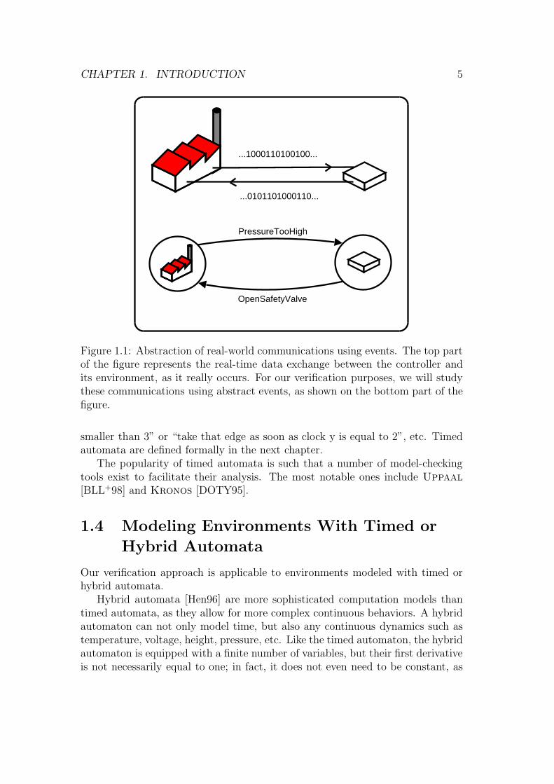
For example, consider a controller interacting with a valve, which needs tobe operated to regulate the air-pressure of a tank. The software controller isaware of the current air-pressure by using an input-sensor and is linked to thevalve by an output port. The valve control chip periodically reads an integervalue on its input port and changes the valve opening angle accordingly, in real-time. In this situation, the control software operates by monitoring an integerinput value and changing an integer output value accordingly. Our verificationmethodology will not manipulate these values directly, but rather abstract themwith events. In this case, the output command could be abstracted by a singleChangeValveAperture event, and our verification process will be able to verify thatit is issued by the controller appropriately. The rationale behind this abstractionis that (1) it greatly simplifies the design of the controllers and (2) that once ithas been proven that the right command is always emitted at the right time,it is always possible to prove that the actual contents of that command is alsoappropriate, if need be. This latter verification would need other techniqueswhich are beyond the scope of this work, so we will not discuss them further.The abstraction of controller-environment communication is illustrated at figure1.1.
By abstracting the inputs and outputs of our software controllers with events,it is possible to design and analyze them in a natural way by using language the-ory. Hence, we will model the software control-logic with automata. Likewise, wewill construct models for the environments using automata, and study the systemas a whole, using the composition of the controller and environment automata.
1.3 Modeling Real-Time Controllers with Timed
Automata
Since we need to design and verify control logics with real-time requirements,finite-state machines (regular languages) do not suffice in our context. We willneed a more powerful computation model to analyze real-time software con-trollers, namely the timed automaton.
Timed automata have been introduced in [AD94], as an extension to regularautomata incorporating the notion of time, and have been widely adopted in theresearch community as a tool for modeling real-time systems. A timed automatonis a finite-state machine augmented with a finite number of clocks. These clocksare real-valued variables which are used to count time and thus have a firstderivative equal to one. They are used to restrict the possible behaviors of theautomaton, by adding timing constraints to its nodes and edges. For example itis possible to express behaviors such that “stay in that location while clock x is
CHAPTER 1. INTRODUCTION 5
PressureTooHigh
OpenSafetyValve
...1000110100100...
...0101101000110...
Figure 1.1: Abstraction of real-world communications using events. The top partof the figure represents the real-time data exchange between the controller andits environment, as it really occurs. For our verification purposes, we will studythese communications using abstract events, as shown on the bottom part of thefigure.
smaller than 3” or “take that edge as soon as clock y is equal to 2”, etc. Timedautomata are defined formally in the next chapter.
The popularity of timed automata is such that a number of model-checkingtools exist to facilitate their analysis. The most notable ones include Uppaal[BLL+98] and Kronos [DOTY95].
1.4 Modeling Environments With Timed or
Hybrid Automata
Our verification approach is applicable to environments modeled with timed orhybrid automata.
Hybrid automata [Hen96] are more sophisticated computation models thantimed automata, as they allow for more complex continuous behaviors. A hybridautomaton can not only model time, but also any continuous dynamics such astemperature, voltage, height, pressure, etc. Like the timed automaton, the hybridautomaton is equipped with a finite number of variables, but their first derivativeis not necessarily equal to one; in fact, it does not even need to be constant, as

CHAPTER 1. INTRODUCTION 6
hybrid automata define their continuous dynamics with differential equations.The tank environment of the previous section for example, could be modeled
elegantly with a hybrid automaton. It would have a variable representing thepressure of the tank, with each discrete location enforcing a particular pressuredynamics (indicating how fast the pressure rises when the valve is closed, forinstance). With an environment modeled this way, it is possible to verify formallythat the pressure variable will never reach some critical threshold for example.
Unlike with timed automata, the analysis of hybrid automata turns out tobe undecidable in the general case1. This is immediate, because we do not knowhow to solve differential equations in general. To work around this undecidability,several subclasses of hybrid automata have been studied, most notably the rect-angular hybrid automaton. The study of these subclasses has made it possible toanalyze hybrid automata with the help of automated tools. These tools includefor example HyTech [HHW97] and Phaver [Fre05].
In this work we will restrict ourselves to the use of timed automata. However,our methodology is completely applicable to environments modeled with hybridautomata.
1.5 Synchrony Hypothesis
Many approaches to the software verification problem use what is usually referredto as the synchrony hypothesis. When making that hypothesis we assume thatthe hardware on which our software controller will run is perfect in the followingsense :
1. The synchrony hypothesis assumes an infinitely fast hardware. This impliesthat (1) any computation can be done in zero time units, and (2) that thecontroller can read input data and emit output commands instantaneously.
2. It also assumes that clock rounding errors never happen; this is essentiallythe same as requiring hardware clocks of infinite precision.
3. Finally, it assumes that the hardware clocks do not drift. A drifting clockis a digital clock which sometimes “looses” a tick, yielding inaccurate timereadings. No real-world clock has a drift of zero, even the most sophisticatedatomic clocks do drift (albeit very slowly).
The reason why such an unrealistic hypothesis is used is that (1) it greatlysimplifies the design and analysis of software systems and (2) that in many situa-tions the execution times and rounding errors are just too small compared to thescale of the environment. Indeed, if every delay or time lapse is of several orders
1By analysis of timed or hybrid automata, we mean reachability analysis unless otherwisestated.

CHAPTER 1. INTRODUCTION 7
of magnitude smaller than any time constraint required by the environment, theycan be safely ignored.
However, clearly there are cases where making the synchrony hypothesis isjust too unrealistic. In those circumstances, we have to make sure that the soft-ware will run appropriately, even on hardware with limited speed and relativelyunreliable clocks.
One way of achieving this verification is to study the target hardware plat-form, and incorporate its limitations into the controller model. This can be quitedifficult and time consuming, and the result might only be valid for one platform.
Another approach has been studied by Raskin et al. in [DDR05b], whichworks by using the synchrony hypothesis for the design of the controller, andby formally validating that hypothesis during the verification phase. This isachieved by using a special semantics for the controller automaton, called theAlmost ASAP semantics. This approach is studied in detail in chapter 3.
1.6 Syntax and Semantics
The theoretical aspects of this work will rely heavily on the dual notions of syntaxand semantics. In this work, what we call syntax is a formal definition of a set oflegal objects. The syntax definition indicates which are legal objects and whichare not. For example, the syntax of regular expressions is such that (a+ b(cd)∗)and ((ab)+c) are considered legal, while ((ab)a) and ((acd)+)) are not.
A syntax definition alone is meaningless without an associated semantics. Thesemantics definition creates a formal object, the form of which depends on thesyntax. To continue with regular expression, the semantics of (a+ b(cd)∗), whichwe note [[(a + b(cd)∗)]] is the set of strings : {a, b, bcd, bcdcd, bcdcdcd, . . .}.
The advantage of distinguishing syntax and semantics is clear : it is muchmore convenient to write (ab)∗(cd)∗ + e+f , than {ǫ, ab, abab, ababab, . . . , cd, cdcd,cdcdcd, . . . , abcd, ababcd, abababcd, . . . , abcdcd, abcdcdcd, . . . , ef, eef, eeef, . . .}.
Moreover, the latter description is not only heavy and difficult to understand,it is also ambiguous2. This is why we use syntax definitions; to represent complex(and possibly infinite) mathematical objects (which are ultimately described bythe semantics) in a concise and unambiguous manner.
In this work, we will not use regular expression to reason on software con-trollers, but rather timed automata and timed transition systems. Timed au-tomata will provide syntax to our models, and we will define their semantics inthe form of timed transition systems. As with timed automata, timed transitionsystems will be discussed in the next chapter.
2This example is a bit overdone to stress the point. It is of course possible the express thelanguage of the regular expression above in a totally unambiguous fashion.

CHAPTER 1. INTRODUCTION 8
1.7 AASAP Semantics and Implementability
As stated previously, the Almost ASAP semantics provides a means to formallyvalidate the synchrony hypothesis. This approach works as follows :
1. A model for the controller is designed, using timed automata. At thispoint, we do not worry about the limitations of the hardware yet. Thisallows the designer to focus on control logic rather than implementationdetails, yielding simpler and more elegant models.
2. When the controller automaton and environment automata have been cre-ated, they are analyzed in the classical way by composing both automataand applying model-checking techniques. This analysis is made using thestandard semantics for timed automata, which does not forbid unimple-mentable behaviors. A sequence of actions is considered unimplementablein our context, if it cannot be executed by hardware, no matter how fast itis or how precise its digital clocks are. These behaviors include for example :taking several discrete transitions consecutively, without letting time elapse;or taking transitions only at fixed points in time (this is unimplementablebecause it requires infinite clock-precision). Thus, this preliminary analy-sis can yield “correctness proofs” for controllers which cannot be used inpractice.
3. To make sure that the control strategy can be be executed by hardware,we analyze the system a second time, but with this time using the Al-most ASAP semantics for the controller. Using this semantics, it is bepossible verify (with the help of automated tools) the correctness and im-plementability of control strategies expressed with timed automata3.
The reader might wonder why the second step is necessary. In fact, it is not.However, as analyzing the classical semantics of timed automata is much fasterthan with the Almost ASAP semantics, that second step is very useful in practice(because if it fails, the next step will certainly fail as well).
1.8 Implementing Controllers Systematically
We have stated earlier that one of the advantages of the top-down verification ap-proach is that it is possible to create implementations in a systematic way. Withthe Almost ASAP semantics approach, this is achieved using an implementationsemantics.
3Actually, the Almost ASAP semantics is not exactly applied on timed automata but ratheron one of its subclass, called Elastic controllers. The difference is quite small however, andwill be detailed in the following chapters.

CHAPTER 1. INTRODUCTION 9
Once the control-logic of the controller has been proven correct and imple-mentable, we give a third semantics to the controller’s timed automaton, whichdoes not only describe what the controller does, but also contains details onhow this is achieved in practice. The purpose of the three semantics we havementioned can be summarized as follows :
• The classical semantics enables us to ensure that a control strategy is soundin the context of the synchrony hypothesis.
• The Almost ASAP semantics enables us to verify that a control strategyremains sound, even when executed on hardware with limited speed andprecision.
• The implementation semantics describes how the control strategy is exe-cuted by hardware and enables us to construct implementations in a sys-tematic way.
In [DDR05b], Raskin et al. have demonstrated how their methodology canbe used to create implementations in a systematic manner, by using a proof-of-concept implementation semantics, which they called program semantics. Theysuccessfully applied this methodology in practice, by creating a code generatingtool4 for the Lego Mindstormstm platform.
1.9 Goal and Structure of this Work
The goal of this work is to study how the Almost ASAP semantics approach canbe applied to more realistic embedded real-time platforms. The implementationsemantics described in [DDR05b] has been voluntarily kept simple, and thusmakes almost no hypothesis about the target run-time environment. As we willsee in the following, the Almost ASAP semantics approach can be improved if weassume that the generated code will run on a hard real-time operating system.Our work will be structured as follows :
• In chapter 2, we define timed automata and their classical semantics. Wewill see how these automata are suitable for the design and analysis ofreal-time software and how this is done in practice.
• In chapter 3, we define the Almost ASAP semantics and the various defini-tions needed for its use. We will keep a to-the-point approach, by reviewingonly the essential aspects which will be needed in this work.
4The tool is available at http://www.ulb.ac.be/di/ssd/madewulf/aasap/

CHAPTER 1. INTRODUCTION 10
• In chapter 4, we define the Program Semantics, as described in [DDR05b].This definition will be followed by a discussion analyzing how it can be im-proved in the context of real-time operating systems. We will then definea new implementation semantics, called unsurprisingly Real-Time Seman-tics, which takes advantage of the capabilities of an RTOS. To validate thisnew semantics formally, we provide a complete simulation proof with theAlmost ASAP Semantics.
• In chapter 5, we present a modern hard real-time operating system, namelyRTAI5. We briefly describe its architecture and a small subset of its API(this information is needed in the following chapter).
• In chapter 6, we present Spectre, a tool for generating provably correctreal-time code which has been created to demonstrate the practical appli-cability of our work. We describe how a Spectre-generated controller usesthe RTAI run-time environment to behave consistently with the Real-TimeSemantics. We also describe the tool’s input language, along with detailsillustrating how it generates code and in what respect this code can beconsidered provably correct.
• In chapter 7, we illustrate the use of Spectre with a case-study.
• In chapter 8, we conclude this work by a discussion reviewing the progressmade in this work, and pointing out some suggestions as to how it couldbe improved.
• Appendix A contains the grammar of the Spectre input language.
• Appendix B contains an example of a Spectre-generated controller.
5RTAI is freely available for download at http://www.rtai.org

Chapter 2
Timed Automata
This chapter introduces the theoretical background needed for the following chap-ters. Definitions are given for timed automata, as well as a number of their usefulproperties. In the final part of the chapter, we show how these computation mod-els can be used in practice with a couple examples.
2.1 Syntax of Timed Automata
Timed automata are finite state automata extended with a finite number of clocks.When a timed automaton (TA) stays in one particular location, each of his clocks’value increases continuously with first derivative equal to one. As a discretetransition occurs, the TA can either reset a clock to zero, or leave it untouched.Before the formal definition, here is a small example of a timed automaton :
Figure 2.1: Simple example of a timed automaton.
11

CHAPTER 2. TIMED AUTOMATA 12
This simple timed automaton has four locations and one clock : t. As indi-cated by the small arrow in the upper left part of the figure, location 1 is theinitial location of this automaton. Three of the four transitions are labeled with astring; they materialize events that occur in the system. Labels and events will betreated in depth later in this chapter. Transition 2 → 4 assigns the clock t to thevalue zero. Thus, while in location 4, the value of clock t increases continuouslyfrom zero onward. Exactly three time units later, t will hold the value 3 and thetransition 4 → 1 will be enabled, because the predicate attached to it becomestrue. When one of its transition becomes enabled a timed automaton can takethat transition as long as it stays enabled. It is important to note that a TA doesnot have to take an enabled transition, and this often leads to non-deterministicbehaviors. In this particular case, the automaton is fully deterministic thanksto the predicate attached to location 4. The automaton cannot refuse to firetransition 4 → 1 when t equals 3 without violating the predicate t ≤ 3.
Synchronization labels
The edges of timed automata are sometimes tagged with strings. Their purposecan be purely informational (as in the example of figure 2.1), or they can be usedto synchronize events with other automata. When modeling complex interactingsystems, it is often convenient to model each system separately with its ownTA. Then, a special operation called synchronized product (also called parallelcomposition in the literature) makes one big timed automaton with all the smallones. The synchronization labels provide a means of communication between theautomata within the composition. This is best illustrated by an example.
The example of figure 2.2 is a much simplified version of the ICMP1 protocol.One station sends a “ping” packet to the other, which in turn responds with an“echo” reply. Observe that not all labels are used to synchronize the sender withthe receiver : the label Timeout is not seen by the receiver. Throughout thiswork, we will use the popular convention of adding an exclamation mark afteroutput messages, and a question mark after input messages. As illustrated bythe figure, the synchronized product is a somewhat natural operation.
Guards and rate conditions
The control flow in timed automata is coerced by the predicates attached to itslocations and edges. The edge predicates are often called guards in the literature.When a guard becomes true, the corresponding edge is said to be enabled and theautomaton can follow that edge as long as it stays enabled. Location predicatesare also often called invariant predicates in the literature. A timed automatoncannot be in a location unless its invariant predicate is true, and must thus leaveits location whenever it becomes false. In the example of figure 2.2, the receiver
1ICMP stands for Internet Control Message Protocol.

CHAPTER 2. TIMED AUTOMATA 13
Figure 2.2: Illustration of synchronization labels and parallel composition.

CHAPTER 2. TIMED AUTOMATA 14
automaton can delay the “echo” up to beta time units, as it can take transition4 → 3 without restriction (it is always enabled because its predicate is true2).It may not stay longer, however, without violating the invariant predicate oflocation 4.
Syntax definitions
Before defining the timed automaton, we need to precise what kind of predicatescan be used in their definition. We will use a notion similar to the one intro-duced in [AD94], namely the rectangular clock predicate. Basically, with thesepredicates it is only possible to compare a clock to a positive rational value, or toa rational interval (possibly infinite). It is not permitted to compare two clocksdirectly for example. Here is the formal definition.
Definition 1 [Rectangular Clock Constraint / Predicate] A rectangular clockconstraint over a set of clocks X is a formula of the form x ∈ I, where I is arational interval, open or closed and possibly infinite. Formally, I is of the form(a, b), [a, b), (a, b], or[a, b] with a, b ∈ Q≥0 ∪ {+∞} and a ≤ b.
A rectangular clock predicate is a finite set of rectangular clock constraints.For a rectangular clock predicate p and a clock valuation v, we write v |= p ifv(x) ∈ I for every “x ∈ I” appearing in p. Finally, the set of all rectangularclock predicates over a clock set X is noted Rect(X), and that same set but withclosed intervals is noted Rectc(X). �
Note that this definition is quite restrictive. It is not possible to express adisjunction directly with one predicate for instance. These restrictions are madeto reduce the complexity of timed automata analysis. This phenomenon is wellknown : models that are too expressive quickly become undecidable. It is shownin [AD94], for instance that allowing to compare a rational value to the sum oftwo clocks leads to undecidability of timed automata analysis.
We are now ready to define the timed automaton formally.
Definition 2 [Timed Automaton - Syntax] A timed automaton is a tuple 〈Loc, l0,Var, Inv, Labin, Labout, Labτ ,Edg〉 where :
• Loc is a finite set of locations.
• l0 ∈ Loc is the initial location.
• Var is a finite set of clocks, which are positive real-valued variables.
• Lab = Labin∪Labout∪Labτ is a structured, finite alphabet of synchronizationlabels. It is partitioned into input output and internal labels, respectively.
2Predicates that evaluate to true are omitted in the figures.

CHAPTER 2. TIMED AUTOMATA 15
• Edg ⊆ Loc × Loc × Rect(Var) × Lab × 2Var is a finite set of edges, alsocalled transitions. The edge (l1, l2, g, σ, R) goes from location l1 to l2, re-sets the clocks contained in R to zero and is enabled only when the clockguard g is true. Depending on the label σ attached to the edge, the tran-sition represents the acceptance of an input (σ ∈ Labin), the emission ofoutput(σ ∈ Labout), or an internal event (σ ∈ Labτ ).
�
2.2 Classical Semantics of Timed Automata
As mentioned in the introduction, the above syntax definition does not meanmuch without an associated semantics. As we will define several semantics fortimed automata in this work (four in total), we will give a name to each to avoidambiguity. We start by defining the classical semantics of timed automata.
Timed transition systems
To formalize the semantics of timed automata we will use timed transition systems(TTS). The TTS associated to a timed automaton captures two things : (1) thecomplete state space of the TA, and (2) for each state of that space, the TTS tellswhich states are reachable in one move3. The state space of a timed automatonis the set of all configurations it can have, i.e. its current location and the valueof its clocks. As the clocks take their values from a dense set, the state space isalmost always infinite4.
Definition 3 [Timed Transition System] A timed transition system T is a tuple〈S, ι,Σ,→〉 where :
• S is a (possibly infinite) set of states.
• ι ∈ S is the initial state.
• Σ is a finite set of labels.
• →⊆ S × Σ ∪ R≥0 × S is the transition relation with R≥0 being the set{x ∈ R | x ≥ 0} of all non-negative real numbers.
�
3In this context, a move is understood as either a discrete jump or an arbitrarily small timeincrement.
4One could make a timed automaton which never lets time elapse, by taking an infinitenumber of transitions at time zero. Then indeed, the state space of that automaton would befinite.

CHAPTER 2. TIMED AUTOMATA 16
Timed transition systems are very useful because they contain in a somewhatconcise manner all the possible behaviors of a timed system. This notion ofpossible behavior is formalized by a path, and is defined as follows :
Definition 4 [Path in TTS] A finite path in the timed transition system T =〈S, ι,Σ,→〉 is a finite sequence alternating between state and transition labels,and is noted λ. Let λ = (s0, τ0, s1, τ1, . . . , τn−1, sn). λ is a finite path of T if (1)for every i ∈ [0, n], si ∈ S and (2) for every i ∈ [0, n), (si, τi, si+1) ∈→. The lengthof λ is n + 1 and is denoted | λ | . This definition is extended to infinite pathsin the obvious way and the length of such a path is +∞. A path λ is initial if itsfirst state is the initial state. We write PathF(T ) the set of all finite initial pathsof T and Path∞(T ) the set of all infinite initial paths of T . The set of stateswhich appear in λ is noted State(λ) �
Now we can define the useful notion of reachability in TTS :
Definition 5 [state-reachability in TTS] Let T = 〈S, ι,Σ,→〉 be a timed tran-sition system and a state s ∈ S. The state s is reachable in T if there exists afinite initial path λ = (s0, τ0, s1, τ1, . . . , τn−1, sn) such that sn = s. The set of allreachable states in T is noted Reach(T ). �
As stated in the introduction, the verification process we employ requires acomposition of the interacting system models. We cannot perform this composi-tion at the syntax level because the environment and controller semantics will notbe the same. Hence, we need a way of composing timed transition systems. Thiscomposition requires a partitioning of the synchronization labels into three sets,so we refine our definition of TTS with a definition of structured timed transitionssystems.
Definition 6 [Structured Timed Transition System] A structured timed transi-tion system (STTS) T is a tuple 〈S, ι,Σin,Σout,Στ ,→〉 where :
• S is a (possibly infinite) set of states.
• ι ∈ S is the initial state.
• The set of labels is partitioned into input (Σin) output (Σout) and internallabels (Στ ).
• →⊆ S × Σin ∪ Σout ∪ Στ ∪ R≥0 × S is the transition relation.
�
Before formalizing the notion of composition mentioned earlier, we need totake a few precautions. We have seen that timed automata communicate throughsynchronization on common labels. This communication is blocking and we need
CHAPTER 2. TIMED AUTOMATA 17
to make sure that (1) no automaton deliberately refuses an input from anotherand (2) no automaton sends an output to one that cannot receive it. These issuesare resolved by imposing input enabledness of the STTS.
Definition 7 [Input Enabled STTS] A STTS T = 〈S, ι,Σin,Σout,Στ ,→〉 is inputenabled if it can accept any input symbol, at any time. Formally, T must be suchthat for all σ ∈ Σin, for all s1 ∈ S there exists s2 ∈ S such that (s1, σ, s2) ∈→.
�
We are now ready to define the composition of two STTS. Note that thisdefinition can be extended to the composition of any number of STTS.
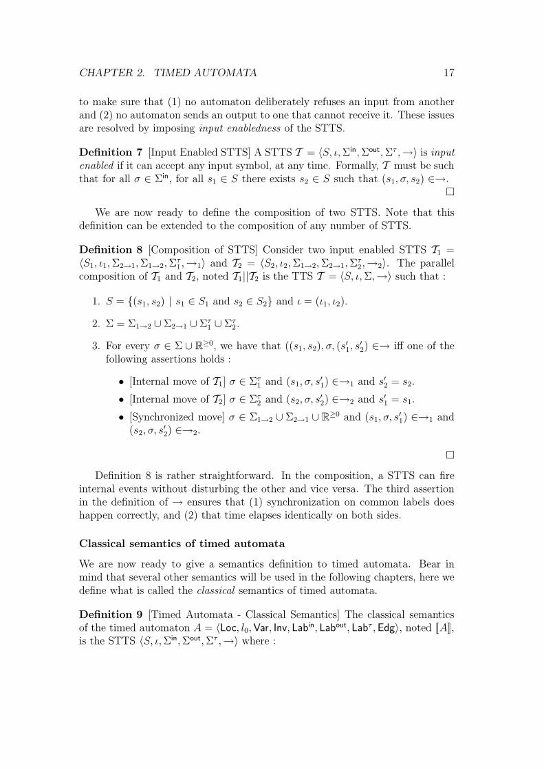
Definition 8 [Composition of STTS] Consider two input enabled STTS T1 =〈S1, ι1,Σ2→1,Σ1→2,Σ
τ1,→1〉 and T2 = 〈S2, ι2,Σ1→2,Σ2→1,Σ
τ2,→2〉. The parallel
composition of T1 and T2, noted T1||T2 is the TTS T = 〈S, ι,Σ,→〉 such that :
1. S = {(s1, s2) | s1 ∈ S1 and s2 ∈ S2} and ι = (ι1, ι2).
2. Σ = Σ1→2 ∪ Σ2→1 ∪ Στ1 ∪ Στ
2.
3. For every σ ∈ Σ ∪ R≥0, we have that ((s1, s2), σ, (s′1, s
′2) ∈→ iff one of the
following assertions holds :
• [Internal move of T1] σ ∈ Στ1 and (s1, σ, s
′1) ∈→1 and s′2 = s2.
• [Internal move of T2] σ ∈ Στ2 and (s2, σ, s
′2) ∈→2 and s′1 = s1.
• [Synchronized move] σ ∈ Σ1→2 ∪ Σ2→1 ∪ R≥0 and (s1, σ, s′1) ∈→1 and
(s2, σ, s′2) ∈→2.
�
Definition 8 is rather straightforward. In the composition, a STTS can fireinternal events without disturbing the other and vice versa. The third assertionin the definition of → ensures that (1) synchronization on common labels doeshappen correctly, and (2) that time elapses identically on both sides.
Classical semantics of timed automata
We are now ready to give a semantics definition to timed automata. Bear inmind that several other semantics will be used in the following chapters, here wedefine what is called the classical semantics of timed automata.
Definition 9 [Timed Automata - Classical Semantics] The classical semanticsof the timed automaton A = 〈Loc, l0,Var, Inv, Labin, Labout, Labτ ,Edg〉, noted [[A]],is the STTS 〈S, ι,Σin,Σout,Στ ,→〉 where :

CHAPTER 2. TIMED AUTOMATA 18
• S = {(l, v) | l ∈ Loc and v is a valuation of the clocks in Var such thatv |= Inv(l)}.
• ι = (l0, v0) with v0 being a valuation of the clocks in Var assigning the valuezero to each clock.
• Σin = Labin,Σout = Labout,Στ = Labτ .
• For every σ ∈ Σin ∪ Σout ∪ Στ ∪ R≥0, the transition ((l, v), σ, (l′, v′)) ∈→ iffone of the following assertions holds :
– σ ∈ Σin ∪ Στ ∪ Σout and there exists an edge (l, l′, g, σ, R) ∈ Edg withv |= g and v′ being the same valuation than v but assigning the valuezero to the clocks in R.
– The edge mentioned above doesn’t exist, σ ∈ Σin and (l′, v′) = (l, v).
– σ ∈ R≥0, l′ = l and for each clock x ∈ Var we have that (1) v′(x) =v(x) + t and (2) ∀t′ ∈ [0, t] : v + t′ |= Inv(l).
�
Notice how definition 9 formalizes the intuitions given previously. The se-mantic state space of the timed automaton (S in the definition) is the set ofall configurations (i.e. location and clock valuation) which satisfy the invariantpredicates. Transitions can occur along enabled edges, which is only the casewhen their guard is satisfied by the current clock valuation. The syntactic com-ponent R of an edge indicates which clocks need to be reset after taking thatedge. A timed automaton can stay in (or enter) a location if and only if thecorresponding location predicate is satisfied. Finally, observe that our definitionof the classical semantics of timed automata is input-enabled : if an input arrivesand no edge specifies what to do, an implicit self-loop occurs (as stated by thesecond assertion in the definition of →).
Illustration of the semantics definition
This definition is essential to the following chapters so we illustrate with anexample. Let A be the timed automaton depicted in figure 2.1. The syntax ofthat automaton has not been given formally but it is straightforward. Its classicalsemantics is the STTS [[A]]= 〈S, ι,Σin,Σout,Στ ,→〉 where :
• S = {(l, v) | l ∈ {1, 2, 3}, v(t) ∈ [0,+∞)} ∪ {(4, v) | v(t) ∈ [0, 3]}
• ι = (1, v0) with v0(t) = 0
• Σin = Σout = φ, Στ = {ǫ,EnterPassword,BadPassword,PasswordOK}

CHAPTER 2. TIMED AUTOMATA 19
• → = {((1, v),EnterPassword, (2, v)) | v(t) ∈ [0,+∞)}∪ {((2, v),PasswordOK, (2, v)) | v(t) ∈ [0,+∞)}∪ {((2, v),BadPassword, (4, v′)) | v(t) ∈ [0,+∞), v′(t) = 0}∪ {((4, v), ǫ, (1, v)) | v(t) = 3}∪ {((l, v), δ, (l, v + δ)) | δ ∈ R≥0, l ∈ {1, 2, 3}, v(t) ∈ [0,+∞)}∪ {((4, v), δ, (l, v + δ)) | δ ∈ R≥0, v + δ(t) ∈ [0, 3]}
2.3 Timed Systems Analysis
When using timed automata to analyze a timed system, we are generally in-terested not only by the model itself but by the formal properties that can beinferred from it. For example, an interesting property of the automaton of figure2.1 could be phrased as “A brute-force attack of n password attempts requiresat least 3n time units”. Of course, we usually want to be more formal and thissection will show how properties are defined and used in practice.
Formal specifications have many kind of properties and this work will mainlyfocus on one kind : safety properties. A safety property requires a formal systemto stay in a predefined subset of the state space, which is usually referred as thesafe states or good states. These kind of properties are very useful in practiceand suffice for many applications. One notable exception where safety propertiesare not enough is the liveness (or fairness) type of property, which requires themodel to actually do what it is supposed to, in a finite amount of time, and tohave no deadlock5.
To define safety properties formally, we need to extend the notion of reacha-bility of definition 5 to regions. A region of a timed transition system is a subsetof its state space. A region R is reachable in the TTS T if R ∩ Reach(T ) 6= φ.
Definition 10 [Safety Property in TTS] Let T = 〈S, ι, σ,→〉 and let R ⊆ S bea region representing a set of good states. T is safe for R iff Reach(T ) ⊆ R.
�
In practice, we use algorithms which compute Reach(T ), and determine ifthat set has an intersection with the complement of R in S. The set R = S \ Ris often called the set of bad states.
To formalize properties in a natural way, we usually use what is called amonitor automaton. This automaton usually consists of two states : Good andBad with one edge going from the first to the second. On that edge we attach apredicate corresponding to the negation of the property we want to verify. Thatmonitor automaton is then included in the composition, along with the otheragents in the system and we compute a reachability analysis to verify if indeed
5Indeed, a model which sits forever in its initial state (provided that state is safe) triviallysatisfies any safety property. This is usually easily detected, however, and does not always needto be verified formally.

CHAPTER 2. TIMED AUTOMATA 20
Bad is never reachable. Of course, some safety properties will be complex enoughso that they cannot be expressed with only one clock predicate, and in that casea bigger monitor automaton will be needed.
For example, to formalize the property mentioned previously, the monitorautomaton of figure 2.3 would work. To express the property accurately, it needsthree states.
PasswordOK ?Bad
Good1
BadPassword ?c := 0
c = 3
c <= 3
Good2
Figure 2.3: Example monitor automaton.

CHAPTER 2. TIMED AUTOMATA 21
2.4 Timed Automata in the Literature
This chapter only scratched the surface of the theory of timed automata. To keepthis work at a reasonable size, we have only given the few definitions needed forthe understanding of the following chapters. We have not described, for instance,how timed automata can be analyzed effectively using automated tools. Thisinformation, along with decidability results, can be found for example in [BY04]and [AD94].

Chapter 3
Implementability of TimedControllers
The final goal of this work is to develop a methodology for building real-timeembedded software with formal assurance that it will work as intended. In theprevious chapter, we have seen that timed automata can be used to provide amodel for the controller and its environment and that it is possible to obtainformal assurance that this model is correct, in the sense that it satisfies someformal requirement.
However, as stated in the introduction, this proof of correctness is only valid inthe context of the synchrony hypothesis. This is because the classical semanticsof timed automata allows unimplementable behaviors. Consider the followingcontroller :
Figure 3.1: This timed automaton has a classical semantics that is not imple-mentable because it requires an infinite clock precision, which any hardware isincapable of.
This controller is obviously not implementable and it illustrates one reason
22

CHAPTER 3. IMPLEMENTABILITY OF TIMED CONTROLLERS 23
for this : any computer hardware has clocks with finite precision. The clocks oftimed automata take their values from a dense set, whereas hardware clocks arealways discrete and thus have limited precision. If the correctness of a controlstrategy relies on infinite time precision, then it will not be implementable. Weneed to make sure that clock-rounding errors will not induce bad behaviors ofthe controller.
Infinite clock precision is not the only cause of unimplementability, as illus-trated by this controller :
Figure 3.2: This second example illustrates the unimplementability caused bythe instantaneity required by the classical semantics. The classical semantics oftimed automata requires that these two transitions be taken in zero time unitswhich is impossible on any hardware.
This last example does not require infinite clock-precision (even digital clockscan hold an exact null value) and yet it is not implementable. This is becauseuntil now we have considered that the communication between the interactingcomponents of the system was instantaneous. This is very convenient at themodeling level, but again it needs to be formally validated. Communications inreal implementations will always introduce delays and we need to make sure thatthe control strategy remains correct when they happen.
The synchrony hypothesis can be seen as an undesirable “side-effect” of theclassical semantics of timed automata. This problem could be solved by taking thehardware limitation into account in the controller design process. This amountsto make syntactic changes to the controller automaton, by adding enough nodes,clocks, predicates and edges in order to obtain a implementable model.
The Almost ASAP semantics approach suggests a different path; it incorpo-rates the hardware limitations the target platform by the means of a semanticschange. This is very convenient because it keeps the controller automaton free ofimplementation details.

CHAPTER 3. IMPLEMENTABILITY OF TIMED CONTROLLERS 24
3.1 Overview of the Almost ASAP Approach
Recall the classical semantics of timed automata defined in the previous chap-ter. This semantics interprets the syntax in the most obvious manner; an edgeguarded by the predicate t = 3 can only be taken when t is exactly 3. Simi-larly, the classical semantics makes the emission of an output event correspondto its arrival to the receiver at the exact same time. The idea behind the AlmostASAP semantics is to make an interpretation of the syntax that is more relaxed;by allowing some bounded imprecision on the guard evaluation mechanism, andsome bounded delay during synchronization on common labels, the almost ASAPsemantics makes the control strategy something which can be executed by hard-ware.
The Almost ASAP semantics is parametric, it takes a real-valued parameternoted ∆, which represents a superior bound on both the time-imprecision ofthe hardware and communication delay. This parameter is used throughout thesemantics, extending its possible behaviors to a wider range. For example, withthe AASAP semantics the interpretation of every guard of the automaton isenlarged by the parameter ∆. An edge with a guard predicate t = 3 will betraversable when t ∈ [3 − ∆, 3 + ∆]. So, if the time imprecision of the hardwareis bounded by ∆, the controller implementation will have a chance to take theedge appropriately. The AASAP semantics also makes a distinction between theemission of an event and its arrival. This is done by duplicating event labels :one set corresponds to the emissions, and the other to the actual treatments bythe receivers. When an event is emitted by the environment, the almost ASAPsemantics allows the controller to wait up to ∆ time units before taking thatevent into account. This represents the time needed for the hardware to detectthe event appropriately.
Suppose we have a controller modeled with a timed automaton A. We canprove that [[A]] satisfies some properties, but we cannot do so directly for its almostASAP semantics : [[A]]AAsap
∆ . To be able to analyze the almost ASAP semanticseffectively with the tools and theories available, we need a way of transforming Ainto some A′ such that [[A′]] is somehow similar to [[A]]AAsap
∆ . In this work, we willuse simulations - and the dual notion of refinement - to formalize this similarity.
3.2 Simulation and Controller Refinement
In the previous chapter, we have defined the structured timed transition system,which in our context is used to represent the timed state space of the controllersand environments we want to model. The STTS describes for each state, whichstates are reachable in one transition - discrete or continuous. The possiblebehaviors of an STTS is represented by the set of all its initial paths. Theconcept of simulation is closely related to initial paths; intuitively, an STTS A
CHAPTER 3. IMPLEMENTABILITY OF TIMED CONTROLLERS 25
can simulate another STTS B if every initial path of B is also an initial path ofA. In short, in order for A to simulate B it must have at least as much possiblebehaviors as B. The notion simulation is defined formally by constructing arelation between the state spaces of the two STTS :
Definition 11 [Simulation relation for STTS] Given two STTS,T1 = 〈S1, ι1,Σ
in1 ,Σ
out1 ,Στ
1 ,→1〉 and T2 = 〈S2, ι2,Σin2 ,Σ
out2 ,Στ
2,→2〉, let Σ = Σout1 ∪
Σin1 ∪Στ
1 , we say that T2 is simulable by T1, noted T2 ⊑ T1, if there exists a relationR ⊆ S2 × S1 (called a simulation relation) such that:
• (ι2, ι1) ∈ R;
• for any (s2, s1) ∈ R, for any σ ∈ Σ∪R≥0, for any s′2 such that (s2, σ, s′2) ∈→2,
there exists s′1 ∈ S1 such that (s1, σ, s′1) ∈→1 and (s′2, s
′1) ∈ R.
�
When two STTS can simulate each other, we say that they are mutuallysimilar, but this will not be needed in the following. The similarity we havedefined is sufficient in our context because it preserves safety properties.
To reason on preservation of safety properties, it is convenient to think interms of refinement. The notion of refinement is dual to that of simulation; ifB ⊑ A, i.e. A can simulate B, then we say that B refines A, in the sense thatB has less possible behaviors than A. Safety properties which are satisfied by anSTTS are also satisfied by any refined version of that STTS. In fact, simulationrelations even preserve stronger properties such as the ones that can be expressedwith LTL formulas.
Recall from definition 10 that an STTS T is safe for a region R iff Reach(T ) ⊆R. The preservation of safety properties is formalized as follows :
Theorem 1 Let T1 = 〈S1, ι1,Σin1 ,Σ
out1 ,Στ
1 ,→1〉 , T2 = 〈S2, ι2,Σin2 ,Σ
out2 ,Στ
2,→2〉be two STTS such that T1 ⊑ T 2. If T2 is safe for a region R ⊆ S2 ⊆ S1 then T1
is also safe for R.
This theorem will be extremely useful in the following. Recall that our ulti-mate goal is to generate provably correct code in a systematic fashion. As we haveseen in the introduction, this will require the use of an implementation semantics,which details how the hardware executes the control strategy described by thecorresponding timed automaton. To verify the soundness of the implementationsemantics, we will use simulation proofs. Indeed, if we can prove that an imple-mentation semantics is simulable by the AASAP, then we will not need to verifythe safety of that implementation semantics, thanks to the above theorem. Sucha simulation proof will be given for the Real-Time Semantics in the next chapter.

CHAPTER 3. IMPLEMENTABILITY OF TIMED CONTROLLERS 26
3.3 Elastic Controllers and ASAP Semantics
As seen in the previous chapter, invariant predicates can be attached to thenodes of a timed automaton to force it to leave its location. This was necessaryin order to obtain a controller which does not idle constantly. A simpler wayto work with timed automata is to remove invariants completely and assume anASAP behavior. This ASAP semantics makes the automaton take every actionas soon as possible, thus removing the need for invariant predicates completely.In [DDR05b], controllers are modeled with this subclass of timed automata, andare called Elastic controllers.
Definition 12 [Elastic Controller] An Elastic controller A is a tuple〈Loc, l0,Var, Labin, Labout, Labτ ,Edg〉 where:
• Loc is a finite set of locations;
• l0 ∈ Loc is the initial location;
• Var = {x1, . . . , xn} is a finite set of clocks;
• Lab = Labin ∪ Labout ∪ Labτ is a finite structured alphabet of labels, par-titioned into input labels Labin, output labels Labout, and internal labelsLabτ ;
• Edg is a set of edges of the form (l, l′, g, σ, R) where l, l′ ∈ Loc are locations,σ ∈ Lab is a label, g ∈ Rectc(Var) is a guard and R ⊆ Var is a set of clocksto be reset.
�
Note that Elastic controllers only use closed rectangular predicates. This isbecause in our context of finite clock-precision, comparing a clock to a non-closedrational interval does not make sense.
3.4 Almost ASAP Semantics
Before defining the AASAP semantics we need a couple more definitions:
Definition 13 [True Since] We define the function “True Since”, noted TS :[Var → R≥0] × Rectc(Var) → R≥0 ∪ {−∞}, as follows:
TS(v, g) =
{
t if v |= g ∧ v − t |= g ∧ ∀t′ > t : v − t′ 6|= g−∞ otherwise
�

CHAPTER 3. IMPLEMENTABILITY OF TIMED CONTROLLERS 27
This TS function will be used in the AASAP semantics definition to expressthat the controller must take action when the predicate of an outgoing edge hasbeen true long enough. Recall that the AASAP semantics allows a delay of upto ∆ time units before taking a transition.
To represent the clock imprecision, the guards attached to the edges of theelastic controller are enlarged. This is formalized as follows :
Definition 14 [Guard Enlargement] Let g(x) be the rectangular constraint “x ∈[a, b]”, the rectangular constraint ∆g(x)∆ with ∆ ∈ Q≥0 is the formula “x ∈ [a−∆, b+∆]” if a−∆ ≥ 0 and “x ∈ [0, b+∆]” otherwise. If g is a closed rectangularpredicate then ∆g∆ is the set of closed rectangular constraints {∆g(x)∆ | g(x) ∈g}. �
We are now ready to define the AASAP semantics. Intuitions are given rightafter the definition.
Definition 15 [AASAP semantics] Given an Elastic controller
A = 〈Loc, l0,Var, Labin, Labout, Labτ ,Edg〉
and ∆ ∈ Q≥0, the AASAP semantics of A, noted [[A]]AAsap
∆ is the STTS
T = 〈S, ι,Σin,Σout,Στ ,→〉
where:
(A1) S is the set of tuples (l, v, I, d) where l ∈ Loc, v ∈ [Var → R≥0], I ∈ [Σin →R≥0 ∪ {⊥}] and d ∈ R≥0;
(A2) ι = (l0, v, I, 0) where v is such that for any x ∈ Var : v(x) = 0, and I issuch that for any σ ∈ Σin, I(σ) = ⊥;
(A3) Σin = Labin, Σout = Labout, and Στ = Labτ ∪ Labin ∪ {ǫ};
(A4) The transition relation is defined as follows:
– for the discrete transitions, we distinguish five cases:
(A4.1) let σ ∈ Labout. We have ((l, v, I, d), σ, (l′, v′, I, 0)) ∈→ iff thereexists (l, l′, g, σ, R) ∈ Edg such that v |= ∆g∆ and v′ = v[R := 0] ;
(A4.2) let σ ∈ Labin. We have ((l, v, I, d), σ, (l, v, I ′, d)) ∈→ iff
· either I(σ) = ⊥ and I ′ = I[σ := 0];
· or I(σ) 6= ⊥ and I ′ = I.
(A4.3) let σ ∈ Labin. We have ((l, v, I, d), σ, (l′, v′, I ′, 0)) ∈→ iff thereexists (l, l′, g, σ, R) ∈ Edg, v |= ∆g∆, I(σ) 6= ⊥, v′ = v[R := 0] andI ′ = I[σ := ⊥] ;

CHAPTER 3. IMPLEMENTABILITY OF TIMED CONTROLLERS 28
(A4.4) let σ ∈ Labτ . We have ((l, v, I, d), σ, (l′, v′, I, 0)) ∈→ iff thereexists (l, l′, g, σ, R) ∈ Edg, v |= ∆g∆, and v′ = v[R := 0] ;
(A4.5) let σ = ǫ. We have for any (l, v, I, d) ∈ S : ((l, v, I, d), ǫ, (l, v, I, d))∈→.
– for the continuous transitions:
(A4.6) for any t ∈ R≥0, we have ((l, v, I, d), t, (l, v + t, I + t, d + t)) ∈→iff the two following conditions are satisfied:
· for any edge (l, l′, g, σ, R) ∈ Edg with σ ∈ Labout ∪ Labτ , wehave that:
∀t′ : 0 ≤ t′ ≤ t : (d+ t′ ≤ ∆ ∨ TS(v + t′, g) ≤ ∆)
· for any edge (l, l′, g, σ, R) ∈ Edg with σ ∈ Labin, we have that:
∀t′ : 0 ≤ t′ ≤ t : (d+t′ ≤ ∆∨TS(v+t′, g) ≤ ∆∨(I+t′)(σ) ≤ ∆)
�
Comments on the AASAP semantics definition
(A1) The state space is made of 4-tuples (l, v, I, d). l and v are the locationand clock-valuation as in the classical semantics. I is vector assigning areal value to every input label, representing the time elapsed since the lastuntreated occurrence of that label, or ⊥ if there is no pending occurrence ofthat label. The AASAP semantics does not react instantaneously to inputevents, so it needs to remember how long it has delayed an input. The valued holds the time elapsed since the last location change occurred. That valuewill be used to delay edge crossings; the controller can ignore an enablededge if d is smaller than ∆.
(A2) The initial location definition is straightforward.
(A3) As mentioned previously, the AASAP semantics duplicates input labels.A distinction is made between the emission of an output label σ and itsreception as an input label σ by the controller. When the input is actuallyreceived, it is treated as an internal event, hence Labin is added to Στ .
(A4.1) To cross an edge tagged with an output label, the current clock valuationmust satisfy the corresponding guard predicate, enlarged by ∆. The nota-tion v′ = v[R := 0] means that v′ is the same valuation than v but assigningthe value 0 to the clocks in R. This behavior is exactly the same as in theusual semantics, except for the guard enlargement.
(A4.2) This rule indicates what happens when a label is emitted by the environ-ment. In the normal case, the corresponding value in I is set to zero. If

CHAPTER 3. IMPLEMENTABILITY OF TIMED CONTROLLERS 29
more than one input of the same kind is received before the controller hadthe chance to treat the first one, the semantics simply ignores the othersand the “older” value in I is kept. Note that no edge is crossed at this point,the controller stays in its location for now. Also, this rule alone ensures theinput enabledness of the controller.
(A4.3, 4, 5) These rules should be clear with the previous comments.
(A4.6) The previous rules defined when the controller can take action, this rulestates when it must do so. It can let t time units elapse and not take atransition only if (1) the controller made a location change less than ∆ timeunits ago : d+ t ≤ ∆; or (2) there are no enabled outgoing edge, or if thereare enabled outgoing edges, they have been enabled for less than ∆ timeunits : TS(v + t, g) ≤ ∆. Also, the controller cannot delay the treatmentof an input event more than ∆ time units : (I + t′)(σ) ≤ ∆.
Summary of the Almost ASAP semantics
Let us summarize the previous formal definition. In our methodology, controlstrategies are expressed using a syntax that is free of invariant predicates. Thecontroller always tries to take a transition as soon as it can thus, almost as soonas possible. The “almost” is quantified by the parameter ∆, which is the upperbound on three different delays or time imprecisions :
• The controller can wait up to ∆ time units between two location changes,no matter the outgoing edge guards. This represents the fact that CPUsare not infinitely fast; a “location change” in the real world takes up a fewprocessor cycles. It would be unreasonable to qualify a semantics allow-ing an infinite number of location changes in a finite amount of time asimplementable.
• Since digital clocks aboard real computers have finite precision, every edgeof the controller is enlarged by the value ∆. If clock-rounding errors areguaranteed to be always smaller than ∆, then then controller implementa-tion will be able to cross the edge appropriately in all situations, despitethe imprecision of its clocks.
• Finally, the almost ASAP semantics models communication delays that canbe as large as ∆. Each time an input arrives, the controller can wait up to∆ time units before taking the corresponding edge, thus taking the inputinto account.

CHAPTER 3. IMPLEMENTABILITY OF TIMED CONTROLLERS 30
Example
As with the Classical Semantics, we illustrate the Almost AASAP Semanticsdefinition with an example. Again, we use the timed automaton of figure 2.1but with a minor modification : consider EnterPassword as an input label andBadPassword and PasswordOK as output labels. Also, as we work with an Elasticcontroller this time, the predicate attached to location 4 is removed. To simplifythe notations, consider that the clock valuation v and the input delay vectorI are real values - I can still have the value ⊥. There is only one clock andinput label in this example so this works fine. Finally, in the definition of →,assume that the free variables which are not quantified on the right hand sideof the set definitions are simply non-negative real values. The Almost ASAPsemantics of that Elastic controller is the structured timed transition system[[A]]AAsap
∆ = 〈S, ι,Σin,Σout,Στ ,→〉 where :
• S = {(l, v, I, d) | l ∈ {1, 2, 3, 4}, v, d ∈ R≥0, I ∈ {R≥0 ∪ ⊥}}
• ι = (1, 0,⊥, 0)
• Σin = {EnterPassword},Σout = {EnterPassword,BadPassword},Στ = {ǫ}
• → = {((l, v,⊥, d),EnterPassword, (l, v, 0, d)) | l ∈ {1, 2, 3, 4}} (1)∪ {((l, v, I, d),EnterPassword, (l, v, I, d)) | l ∈ {1, 2, 3, 4}} (2)
∪ {((1, v, I, d),EnterPassword, (2, v,⊥, 0))} (3)∪ {((2, v, I, d),PasswordOK, (3, v, I, 0)) | I ∈ {R≥0 ∪⊥}} (4)∪ {((2, v, I, d),BadPassword, (4, 0, I, 0)) | I ∈ {R≥0 ∪ ⊥}} (5)∪ {((4, v, I, d), ǫ, (1, v, I, 0)) | v ∈ [3 − ∆, 3 + ∆], I ∈ {R≥0 ∪ ⊥}} (6)∪ {((1, v,⊥, d), t, (1, v + t,⊥, d+ t))} (7)∪ {((1, v, I, d), t, (1, v + t, I + t, d+ t)) | I ∈ {R≥0 ∪ ⊥}, I + t ≤ ∆} (8)∪ {((2, v, I, d), t, (2, v + t, I + t, d+ t)) | I ∈ {R≥0 ∪ ⊥}, d+ t ≤ ∆} (9)∪ {((3, v, I, d), t, (3, v + t, I + t, d+ t)) | I ∈ {R≥0 ∪ ⊥}} (10)∪ {((4, v, I, d), t, (4, v + t, I + t, d+ t)) | I ∈ {R≥0 ∪ ⊥}, v + t ≤ 3} (11)∪ {((4, v, I, d), t, (4, v + t, I + t, d+ t)) | I ∈ {R≥0 ∪ ⊥}, d+ t ≤ ∆} (12)
Comments on the discrete transitions
• (1) The controller waits for the input event EnterPassword. When it arrives,I is set to zero but no location change occurs yet. Notice that there isno restriction on the location here; the controller can receive the inputEnterPassword at any time, ensuring input-enabledness.
• (2) As stated by the semantics, the controller ignores the subsequent emis-sions of an untreated input symbol; I and d are left untouched (We knowthat there is an untreated occurrence of the input symbol because I is areal value and not ⊥).

CHAPTER 3. IMPLEMENTABILITY OF TIMED CONTROLLERS 31
• (3) This set of transitions represent what happens when the controller hastaken the input into account. I is reset back to ⊥, d is reset to zero, andthe location changes from 1 to 2.
• (4) There is no guard attached to the edge 2 → 3, so this transition can betaken for any valuation v. It is important to note however, that this doesnot mean that the controller can delay the emission indefinitely; at somepoint it will have to make that transition when the transition relation →does not allow it to let time pass anymore.
• (5) This works just the same as the previous one, except that we reset theclock valuation as required by the edge 2 → 4.
• (6) The edge 4 → 1 illustrates how the guard enlargement works. Thisedge is enabled as long as the clock valuation satisfies the enlarged guardpredicate.
Comments on the continuous transitions
• (7) Since the only outgoing edge of location 1 corresponds to an input, thecontroller can wait there indefinitely, as long as no input has arrived, i.e.as long as I = ⊥.
• (8) When in location 1, the controller can delay an untreated input for aslong as ∆ time units but not longer.
• (9) When in location 2, the controller faces two outgoing edges that arealways enabled. The classical semantics would require it to fire one of thetwo immediately. Here, we allow the controller to stay in the location 2 foras long as d does not grow larger than ∆.
• (10) As there is no outgoing edge in location 3, the Almost ASAP controllercan of course let time pass indefinitely.
• (11) This one is a little more subtle. The controller can delay the transition4 → 1 for as long as the enlarged guard has not been true for longer than∆ time units. Formally, using the semantics definition, we know that thecontroller can wait t time units if TS(v + t, v + t ∈ [3 − ∆, 3 + ∆]) ≤ ∆,which is equivalent to v + t ≤ 3.
• (12) This is the same as (9), but for location 4.

CHAPTER 3. IMPLEMENTABILITY OF TIMED CONTROLLERS 32
3.5 Almost ASAP Semantics Analysis
We have defined the Almost ASAP Semantics formally and given some intuitionsand examples about why it is useful to ensure implementability. However, asstated previously, the AASAP semantics is not known to model-checking toolsand thus cannot be analyzed “as is”. To work around this difficulty, it is shown in[DDR05b] how to construct a timed automaton with a Classical Semantics thatis simulable by the Almost ASAP semantics of another automaton which can beconstructed effectively. This is formalized by the following theorem :
Theorem 2 For any Elastic controller A, for any ∆ ∈ Q>0, we can con-struct effectively a timed automaton A∆ = F(A,∆) such that [[A]]AAsap
∆ ⊑[[A∆]]and [[A∆]]⊑[[A]]AAsap
∆ .
The interested reader will find all the details of this construction, with fullproofs, in [DDR05b].
Thanks to this theorem, we are able to analyze the Almost ASAP Semanticseffectively. We explain briefly how this is achieved in practice. Suppose we wantto control an environment E to avoid some bad region B, subset of the statespace of the STTS [[E]]. Using the methods introduced in the previous chapter, itis possible to design an elastic controller A and verify formally that [[A]] is safe1
and controls E to avoid B. Now we want to to know if the control strategy Ais implementable. To achieve this, we need to find if there exists some ∆ > 0such that [[A]]AAsap
∆ controls [[E]] to avoid B as well. Hence, we construct thetimed automaton A∆ and analyze it parametrically to verify if there exists apositive rational ∆ such that the control strategy A controls its environment Ein a safe and implementable manner. This parametric analysis can for examplebe computed with the help of HyTech. If no parametric tool is available or if itscomputation does not terminate, it always possible to obtain an approximationof the best ∆ by doing a binary search in the range of possible values. This way,the best ∆ value can be approximated up to any precision.
Our work focuses on the satisfaction of safety properties, but in fact the aboveconstruction could be used to prove the satisfaction of more complex properties,such as LTL (Linear Temporal Logic) formulas or even real-time properties suchas those expressed in MITL (Metric Interval Temporal Logic) or TCTL (TimedComputational Tree Logic).
1It must be mentioned that in this case, [[A]] is understood as the classical semantics of A,but with an ASAP behavior. The classical semantics as defined in the previous chapter cannotbe used “as is” with Elastic controllers.

Chapter 4
Implementation Semantics
The previous chapter introduced a methodology with which we are able to designand validate implementable strategies, using the Almost ASAP Semantics. Butas explained in the introduction, the Almost ASAP Semantics only describeswhat is to be done to keep the environment in a safe state, but contains littleinformation about how a software controller is supposed to achieve this. Weprovide this additional information in an implementation semantics.
We will require the implementation semantics to have the following charac-teristics :
• Parametricity. As the AASAP semantics, the implementation semanticswill need to be parametric. Its parameters will represent the run-timelimitations that the implementation will have to face. This includes clockimprecision, communication delays, CPU speed, etc.
• Almost ASAP Simulability. We will require that the implementationsemantics be simulable by the Almost ASAP semantics. As both semanticsare parametric, the existence of such a simulation relation will depend onthe value of the parameters. As we have seen, STTS refinements preservesafety properties. Thus, if a controller has been proven safe for a positiveAlmost ASAP semantics parameter ∆, then there will exist a set of param-eters (constrained by ∆) such that the implementation semantics will besafe for those parameters.
• Systematic Implementability. This is probably the trickiest part. Theimplementation semantics will need to contain details about how exactlythe software controller will function. We will require it to contain “enoughdetails” in order to be able to create a fully-functional implementation in asystematic fashion. This will be hard to prove formally, so we will need tojustify this with informal arguments.
The rest of this chapter will be organized as follows. First, we will review theproof-of-concept implementation semantics which was introduced in [DDR05b].
33

CHAPTER 4. IMPLEMENTATION SEMANTICS 34
We will see how this semantics satisfies the above requirements, and then identifycertain aspects which could be improved. This discussion will lead to a newimplementation semantics, specially designed to take advantage of the featuresof real-time operating systems.
4.1 Program Semantics
In [DDR05b], Raskin et al. have demonstrated the practical applicability ofthe AASAP semantics with a simple, yet functional, approach. The resultingprogram is composed of an infinite loop which is executed as fast as possible.The body of that loop is called an execution round and it is composed of thefollowing steps :
1. The clock register is read and stored in a global variable.
2. The input sensors are checked and stored in a vector.
3. The outgoing edges of the current location are checked. If one of them isenabled, the edge is taken and the input vector, current location and clockvalues are updated accordingly.
4. The next execution round starts immediately.
This simple implementation scheme has been chosen because it is obviouslyimplementable. Also, this can formalized quite naturally if we make a coupleassumptions; (1) the length of an execution round is bounded by a finite rationalvalue, called ∆L, and (2) the clock register of the CPU (or whichever clock valueis read by the program) is updated every ∆P time units. Using these two values,it is possible to create a formal semantics which is a refined version of the AlmostASAP semantics.
Clock rounding
Before giving a formal definition of the Program Semantics, we need a way toformalize the time-imprecision induced by digital clocks. This is done by usingthe following clock-rounding function, which converts an exact time value intoits corresponding digital value, depending on the clock granularity ∆P :
Definition 16 [Clock rounding] Let T ∈ R≥0 and ∆ ∈ Q>0.⌊T ⌋∆ = ⌊ T
∆⌋∆, where ⌊x⌋ is the greatest integer k such that k ≤ x.
Likewise, ⌈T ⌉∆ = ⌈ T∆⌉∆, where ⌈x⌉ is the smallest integer k such that k ≥ x.
�
From this definition, we obtain the following lemma, which will be used ex-tensively in the following.
CHAPTER 4. IMPLEMENTATION SEMANTICS 35
Lemma 1 For any T ∈ R≥0, any ∆ ∈ Q>0, we have that :
T − ∆ < ⌊T ⌋∆ ≤ T , and
T ≤ ⌈T ⌉∆ < T + ∆.
4.1.1 Formalization of the Program Semantics
In order to prove that this simple implementation strategy is indeed simulableby the Almost ASAP semantics, we need a formal semantics definition for thisstrategy; this is done as follows :
Definition 17 [Program Semantics] Let A be an Elastic controller and ∆L,∆P ∈ Q>0. Let ∆S = ⌈∆L + ∆P ⌉∆P
. The (∆L,∆P ) Program Semantics of A,noted [[A]]Prg
∆L,∆Pis the structured timed transition system T = 〈S, ι,Σin,Σout,
Στ ,→〉 where:
(P1) S is the set of tuples (l, r, T, I, u, d, f) such that l ∈ Loc, r is a functionfrom Var into R≥0, T ∈ R≥0, I is a function from Labin into R≥0 ∪ {⊥},u ∈ R≥0, d ∈ R≥0, and f ∈ {⊥,⊤};
(P2) ι = (l0, r, 0, I, 0, 0,⊥) where r is such that for any x ∈ Var, r(x) = 0, I issuch that for any σ ∈ Labin, I(σ) = ⊥;
(P3) Σin = Labin, Σout = Labout, Στ = Labτ ∪ Labin ∪ {ǫ};
(P4) the transition relation → is defined as follows:
– for the discrete transitions:
(P4.1) let σ ∈ Labout. ((l, r, T, I, u, d,⊥), σ, (l′, r′, T, I, u, 0,⊤)) ∈→ iffthere exists (l, l′, g, σ, R) ∈ Edg such that ⌊T ⌋∆P
− r |= ∆Sg∆S
andr′ = r[R := ⌊T ⌋∆P
].
(P4.2) let σ ∈ Labin. ((l, r, T, I, u, d, f), σ, (l, r, T, I ′, u, d, f)) ∈→ iff
· either I(σ) = ⊥ and I ′ = I[σ := 0];
· or I(σ) 6= ⊥ and I ′ = I.
(P4.3) let σ ∈ Labin. ((l, r, T, I, u, d,⊥), σ, (l′, r′, T, I ′, u, 0,⊤)) ∈→ iffthere exists (l, l′, g, σ, R) ∈ Edg such that ⌊T ⌋∆P
− r |= ∆Sg∆S
,I(σ) > u,r′ = r[R := ⌊T ⌋∆P
] and I ′ = I[σ := ⊥];
(P4.4) let σ ∈ Labτ . ((l, r, T, I, u, d,⊥), σ, (l′, r′, T, I, u, 0,⊤)) ∈→ iffthere exists (l, l′, g, σ, R) ∈ Edg such that ⌊T ⌋∆P
− r |= ∆Sg∆S
and r′ = r[R := ⌊T ⌋∆P].
(P4.5) ((l, r, T, I, u, d, f), ǫ, (l, r, T + u, I, 0, d,⊥)) ∈→ iff either f = ⊤ orthe two following conditions hold:

CHAPTER 4. IMPLEMENTATION SEMANTICS 36
· for any σ ∈ Labin, for any (l, l′, g, σ, R) ∈ Edg, we have thateither ⌊T ⌋∆P
− r 6|= ∆Sg∆S
or I(σ) ≤ u
· for any σ ∈ Labout ∪Labτ , for any (l, l′, g, σ, R) ∈ Edg, we havethat ⌊T ⌋∆P
− r 6|= ∆Sg∆S
– for the continuous transitions:
(P4.6) ((l, r, T, I, u, d, f), t, (l, r, T, I+t, u+t, d+t, f)) ∈→ iff u+t ≤ ∆L.
�
4.1.2 Comments on the Program Semantics
The previous definition is clearly not obvious so we comment the most importantparts.
State space
The state space of this new STTS is a bit more complicated than the one usedwith the AASAP semantics; it is composed of tuples of the form (l, r, T, I, u, d, f).
• l, I, and d have the same meaning they had in the AASAP semantics.
• The value T holds the exact time at which the current execution round wasstarted.
• The function r represents the clock-valuation but it works differently fromthe valuation v of the AASAP semantics. Timed automata can have anynumber of clocks, all containing a different value and increasing simulta-neously. In practice however, there is usually only one clock used, so the“clocks” used by the real-time program are materialized by integer variableswhich, when reset, are assigned to the current clock value (i.e. ⌊T ⌋∆P
). Toobtain a clock’s value1, the value stored in r must be substracted from T .The values stored in r are digital values (as opposed to T ) and are thusalways a multiple of ∆P .
• The variable u holds the exact time elapsed since the beginning of thecurrent execution round. Thus, T + u is always the exact present time.
• The flag f is set to ⊤ when the current execution round ends. It holds thevalue ⊥ at all other times.
1By current clock value, we mean the value of the clock at the beginning of the currentexecution round.

CHAPTER 4. IMPLEMENTATION SEMANTICS 37
Transition relation
Remember that this Program Semantics is meant to be a refined version of theAlmost ASAP semantics. Basically, this implies two things : (1) when the Pro-gram Semantics makes a discrete jump, the AASAP semantics must be able tofollow and (2) when the Program Semantics lets time elapse without making anytransition, the AASAP semantics must be able to do the same. We will notgive the full simulation proof here (as another lengthy simulation proof will bedetailed later), so while explaining the rules of the transition relation, we alsogive insights on how this makes the Program Semantics simulable by the AlmostASAP. The rules which are simple enough are not mentioned.
(P4.1) In the Program Semantics, the guards are enlarged with the value ∆S =⌈∆L + ∆P ⌉∆P
. It is rounded with ∆P because this constant is intendedto be written in real code - to enlarge the edge guards - so it needs tobe expressible in a non-fractional amount of time units ∆P . Observe thatan edge guarded by the predicate g is enabled when ⌊T ⌋∆P
− r |= ∆Sg∆S
.⌊T ⌋∆P
is the value held by the global variable we mentioned previously, andas r, g and ∆S are readily available by the program, this is a computationthat can be made by the software controller.
(P4.3) This rule is self-explanatory, except for the I(σ) > u requirement. Remem-ber that inputs are checked only at the beginning of the execution round, sothe program cannot treat an input which has arrived after the beginning ofthe current round, and must wait until the next one. The value u representsthe time spent into the current round, so it must be strictly smaller thanI(σ) for the program to take the arrival of σ into account in the currentround.
(P4.5) This transition is taken when a new execution round is started. If theprogram has already made an action this round (i.e. f = ⊤) then a newround can start immediately. If not, a new round can start, but only ifthere are no enabled outgoing edges at the current location.
4.1.3 AASAP Simulability of the Program Semantics
In [DDR05b], a simulation proof is given, asserting that the Program Semanticsis simulable by the Almost ASAP semantics, requiring only that ∆P and ∆L aresmall enough compared to ∆. This is stated by the following theorem :
Theorem 3 Let A be an Elastic controller, for any rationals ∆, ∆L, ∆P ∈ Q>0
such that ∆ > 3∆L + 4∆P , we have [[A]]Prg∆L,∆P
⊑[[A]]AAsap∆ .
We omit the proof of this theorem here, but it can be found in [DDR05b].To clarify things a bit, we illustrate the existence of the bound ∆ > 3∆L + 4∆P
with an example.

CHAPTER 4. IMPLEMENTATION SEMANTICS 38
Insights on the bound 3∆L + 4∆P
The following scenario should make the value of this bound on ∆ more clear.Consider an outgoing edge tagged with an output event, and guarded with thepredicate t = 3. In this context, a worst-case scenario is to have ⌊T ⌋∆P
− r(t) =3 − ∆S − ∆P , which is the case when the guard has been missed by exactly oneclock tick. Then, at worst, the edge will be taken at the end of the next round,when TS(t = 3) = 3∆L + 4∆P . The 4∆P term in the expression is the worstrounding-error possible in the guard-evaluation mechanism. The 3∆L term isexplained by (1) the fact the edge is fired 2∆L time units after it is “enabled”and (2) that the the maximum error between r(t) and the exact value of t canbe as large as ∆L (not considering the rounding error which has already beencounted). Remember that the Almost ASAP semantics must take an edge whichhas been enabled for ∆ time units, so this example shows that a simulationrelation cannot exist between the two semantics unless ∆ > 3∆L + 4∆P . Theinterested reader will find the complete proof in [DDR05b].
4.1.4 Implementability of the Program Semantics
At this point it should be clear that, using the Program Semantics, it is possible toconstruct effectively a piece of software which can be considered provably correct.Again, this has been demonstrated successfully in [DDR05a].
4.1.5 Limitations of the Program Semantics
The implementation strategy that we have previously described was meant todemonstrate the usefulness of the Almost ASAP semantics in a practical manner.However, there is still space for improvements left and one of the main objectivesof this work is to create an implementation strategy that could be even moreuseful.
The big downside of the Program Semantics just described is that it imposesa CPU usage of 100%. This is inconvenient for at least three reasons, which wedetail in turn.
1. Multitasking
Clearly, a real-time task requiring a usage of 1 cannot be executed along-sideother tasks. This is unfortunate because there are many cases where real-timeinfrastructures are best designed using many different independent tasks in par-allel. The advantages of a multitask design are numerous :
• Modularity. Compared to monolithic designs, multitasking offers the ben-efit of a greater modularity. Tasks can be added, changed or removed with-

CHAPTER 4. IMPLEMENTATION SEMANTICS 39
out affecting the other tasks (of course, we still need to verify that thereal-time instance stays schedulable when adding and/or changing tasks).
• Simplicity. In many cases, using concurrency can lead to a simpler design,especially if the system needs to perform various, unrelated actions withdifferent levels of importance.
• Fault tolerance. Usually, not all of the code is completely safety-criticaland since most of the attention will have been put on assuring that thecritical part works, the quality of the less important code might be lower.If a non-critical task crashes, it can be restarted without causing a catas-trophe; monolithic systems however, can be brought down by the silliestbug in some relatively unimportant code.
• Performance. If one CPU is not fast enough, make it 2, or even 128 ifneed be ! As the processors’ performance have begun to stall in the lastfew years, the only way to faster software lies in multi-cores, SMP andother multi-tasking hardware technologies. Of course, these require thatthe software be split into parallel tasks.
2. User interaction
The next inconvenience of having a real-time task with a 100% CPU usage is thatit will certainly be very limited in terms of user interaction. The user interfacecode could be built-in, but this is hardly possible in our context of automaticcode generation. Moreover, even if there is only one real-time task running in thesystem, it is very useful to be able to run a background server, which can executetasks which are non-critical and not necessarily real-time.
For example, the real-time platform that was chosen to experiment with thecode generation works this way. RTAI, the Real-Time Application Interface, isa nano-kernel which contains a real-time scheduler that runs a modified versionof the Linux operating system as its idle loop. The real-time system is operatedfrom within Linux. This setup is a very convenient environment; it has all theadvantages of a modern hard real-time OS, along with all the applications andtools available to Linux. However, the architecture of RTAI requires not tolaunch tasks which take up all CPU resources because otherwise Linux won’t beexecuted, leading to a unrecoverable freeze. The architecture of RTAI is describedin chapter 5.
3. Power consumption
In our context of embedded controllers, the power consumption induced by thesoftware execution is not to be overlooked. Embedded applications will oftenrun on batteries, so we need to make sure that the controller does not waste

CHAPTER 4. IMPLEMENTATION SEMANTICS 40
CPU power unnecessarily. In that respect, the Program Semantics can be clearlyimproved.
4.2 Real-Time Semantics
In this section, we introduce a new implementation semantics, which mimics thebehavior of a periodic hard real-time task. It is quite similar to the ProgramSemantics of the previous section, with the notable difference that the beginningof each execution round are evenly spaced in a periodic fashion. This will be theperiod of the real-time task and will be called ∆T . Additionally we require thatevery execution round ends within a fixed time amount, called ∆D, representingthe deadline of the periodic task. Finally, we require that ∆D ≤ ∆T . This isillustrated at figure 4.1.
(1)
(2)
(3)
A B C D
A B C DA C
Program Semantics
Real-Time Semantics
Figure 4.1: Comparison of the Program Semantics and Real-Time Semanticsexecuting four consecutive execution rounds.
The above figure illustrates the respective behaviors of the two implementa-tion semantics when executing four consecutive execution rounds (A,B,C andD). In the Program Semantics, the length of an execution round is bounded by∆L (1). The Real-Time Semantics has much tighter requirements and imposesthat every execution round be started at periodic time intervals ∆T (2). It also

CHAPTER 4. IMPLEMENTATION SEMANTICS 41
requires that every execution round completes within ∆D time units (3). Observefrom the figures that the Real-Time Semantics allows the execution round to bepreempted. This has no consequence, as long as the deadline is always met.
At a first glance, it might seem unnatural to improve a semantics by forcingit to slow down, so we motivate this choice with a few arguments.
Why make the controller idle ?
The answer to that question is simple; the environment does not always needto be watched over a 100% of the time. Consider the following example. AnAlmost ASAP controller has been proven safe, and controls its environement forall values of ∆ < 2 seconds. After implementing the controller, the worst caseexecution time of the execution round is estimated to 10ms and the platform it isrunning on has a clock granularity of 1ms. Using the traditional implementationstrategy, we would obtain a program running the execution round at least 100times per second, which in this case is about 200 times more than what was reallyneeded.
True, the previous argument is not really a strong one, because if we wantedto design controllers with such slow (2 seconds) reaction times, we would not haveneeded to part from the synchrony hypothesis in the first place, and the AASAPmethodology would not be needed. Still, even if we will probably not bring theCPU usage of our controllers from 100% to 0,5% like in the previous example,the gain will lie somewhere in the middle, providing all the advantages we havepreviously mentioned (the possibility of running other tasks and / or running abackground server, consuming less power, etc.).
4.2.1 Overview of the Real-Time Semantics
In practice, the implementation of this new semantics will be quite similar towhat was done with the Program Semantics, except that it explicitly uses somefeatures of a real-time OS. This new implementation strategy is as follows :
• At startup, the controller initializes its variables, and asks the RTOS tocreate a new periodic task with a period of ⌊∆T ⌋∆P
(the period must bean integral number of clock ticks). Usually, the task-creation process in anRTOS is just a matter of indicating which procedure to call when the taskis to be run, and which priority it has. We will call this procedure rt main.
• Every time the task is scheduled, the procedure rt main is invoked2 andperforms the same actions than the body of the execution loop in the Pro-gram Semantics (clock-reading, sensor-checking and edge-crossing, in thatorder).
2Actually, in practice it is not really a procedure call in the traditional sense. Rather, thecontext of the RT task is restored to where it was right before its preemption.
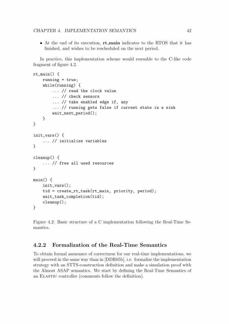
CHAPTER 4. IMPLEMENTATION SEMANTICS 42
• At the end of its execution, rt main indicates to the RTOS that it hasfinished, and wishes to be rescheduled on the next period.
In practice, this implementation scheme would resemble to the C-like codefragment of figure 4.2.
rt_main() {
running = true;
while(running) {
... // read the clock value
... // check sensors
... // take enabled edge if, any
... // running gets false if current state is a sink
wait_next_period();
}
}
init_vars() {
... // initialize variables
}
cleanup() {
... // free all used resources
}
main() {
init_vars();
tid = create_rt_task(rt_main, priority, period);
wait_task_completion(tid);
cleanup();
}
Figure 4.2: Basic structure of a C implementation following the Real-Time Se-mantics.
4.2.2 Formalization of the Real-Time Semantics
To obtain formal assurance of correctness for our real-time implementations, wewill proceed in the same way than in [DDR05b], i.e. formalize the implementationstrategy with an STTS-construction definition and make a simulation proof withthe Almost ASAP semantics. We start by defining the Real-Time Semantics ofan Elastic controller (comments follow the definition).

CHAPTER 4. IMPLEMENTATION SEMANTICS 43
Definition 18 [Realtime Task Semantics] Let A be an Elastic controller and∆T , ∆D, ∆P ∈ Q>0. Let ∆S = ⌈∆T + ∆P ⌉∆P
. The (∆T ,∆D,∆P ) real-timetask semantics of A, noted [[A]]RT
∆T ,∆D,∆Pis the structured timed transition system
T = 〈S, ι,Σin,Σout, Στ ,→〉 where:
(RT1) S is the set of tuples (l, r, T, I, u, d, f) such that l ∈ Loc, r is a functionfrom Var into R≥0, T ∈ R≥0, I is a function from Labin into R≥0 ∪ {⊥},u ∈ R≥0, d ∈ R≥0, and f ∈ {⊥,⊤};
(RT2) ι = (l0, r, 0, I, 0, 0,⊥) where r is such that for any x ∈ Var, r(x) = 0, I issuch that for any σ ∈ Labin, I(σ) = ⊥;
(RT3) Σin = Labin, Σout = Labout, Στ = Labτ ∪ Labin ∪ {ǫ};
(RT4) the transition relation → is defined as follows:
– for the discrete transitions:
(RT4.1) let σ ∈ Labout. ((l, r, T, I, u, d,⊥), σ, (l′, r′, T, I, u, 0,⊤)) ∈→ iffthere exists (l, l′, g, σ, R) ∈ Edg such that ⌊T ⌋∆P
− r |= ∆Sg∆S
andr′ = r[R := ⌊T ⌋∆P
].
(RT4.2) let σ ∈ Labin. ((l, r, T, I, u, d, f), σ, (l, r, T, I ′, u, d, f)) ∈→ iff
· either I(σ) = ⊥ and I ′ = I[σ := 0];
· or I(σ) 6= ⊥ and I ′ = I.
(RT4.3) let σ ∈ Labin. ((l, r, T, I, u, d,⊥), σ, (l′, r′, T, I ′, u, 0,⊤)) ∈→ iffthere exists (l, l′, g, σ, R) ∈ Edg such that ⌊T ⌋∆P
− r |= ∆Sg∆S
,I(σ) > u,r′ = r[R := ⌊T ⌋∆P
] and I ′ = I[σ := ⊥];
(RT4.4) let σ ∈ Labτ . ((l, r, T, I, u, d,⊥), σ, (l′, r′, T, I, u, 0,⊤)) ∈→ iffthere exists (l, l′, g, σ, R) ∈ Edg such that ⌊T ⌋∆P
− r |= ∆Sg∆S
and r′ = r[R := ⌊T ⌋∆P].
(RT4.5) ((l, r, T, I, u, d,⊥), ǫ, (l, r, T, I, u, d,⊤)) ∈→ iff the two followingconditions hold:
· for any σ ∈ Labin, for any (l, l′, g, σ, R) ∈ Edg, we have thateither ⌊T ⌋∆P
− r 6|= ∆Sg∆S
or I(σ) ≤ u
· for any σ ∈ Labout ∪Labτ , for any (l, l′, g, σ, R) ∈ Edg, we havethat ⌊T ⌋∆P
− r 6|= ∆Sg∆S
(RT4.6) ((l, r, T, I, u, d,⊤), ǫ, (l, r, T + u, I, 0, d,⊥)) ∈→ iff u = ∆T .
– for the continuous transitions:
(RT4.7) ((l, r, T, I, u, d,⊥), t, (l, r, T, I+t, u+t, d+t,⊥)) ∈→ iff u+t ≤ ∆D.
(RT4.8) ((l, r, T, I, u, d,⊤), t, (l, r, T, I+t, u+t, d+t,⊤)) ∈→ iff u+t ≤ ∆T .
�

CHAPTER 4. IMPLEMENTATION SEMANTICS 44
Quite not surprisingly, this definition is very similar to the Program Semanticsdefinition. The few differences are detailed in turn.
Comments on the Real-Time Semantics definition
• The worst-case execution time of the execution round ∆L has been replacedwith two distinct parameters ∆T (the period of the real-time task) and ∆D
(its deadline).
• In this semantics, the flag f indicates whether the task is currently idle (⊤)or not idle (⊥). More precisely, ⊤ indicates that the task is waiting to berescheduled at the beginning of the next period. When f = ⊥ the task isactive, but this not necessarily means that it has the CPU; its schedulingstate can be either of ready to run, preempted, or running.
• Rule (RT4.7) says that the task can let time elapse while not finished, untilthe deadline is reached.
• Rules (RT4.8) and (RT4.9) make the task idle until the next period begins.
Real-Time semantics and periodic tasks
The purpose of the Real-Time Semantics is to mimic the behavior of schedulablehard-real time periodic task. We justify this by analyzing the semantics rules :
• Periodicity. Rule (RT4.6) ensures the exact periodicity of the real-timetask.
• Schedulability. The RT semantics behaves as a periodic task which nevermisses a deadline. This is enforced by rule (RT4.7); the flag ⊥ indicatesthat the task has not reached completion yet, which can never be the casewhen u > ∆D
• Preemptability. As said earlier, the Real-Time Semantics allows the taskto be preempted. This is not explicitly indicated in the semantics, becausethe only thing it cares about is that the deadline is reached. When runningother higher-priority tasks, the only thing we have to make sure is that thisperiodic task remains schedulable.
4.2.3 AASAP Simulability of the Real-Time Semantics
The real time semantics is simulable by the Almost ASAP semantics, providedthat their respective parameters satisfy the following inequality :
∆ > ∆T + 2∆D + 4∆P
This is formalized by the following theorem :

CHAPTER 4. IMPLEMENTATION SEMANTICS 45
Theorem 4 (Simulation) Let A be an Elastic controller. For any rationals∆,∆T ,∆D,∆P ∈ Q>0 such that ∆T +2∆D+4∆P < ∆ we have [[A]]RT
∆T ,∆D,∆P⊑[[A]]AAsap
∆ .
Notation Reminder
(l1, r1, T1, I1, u1, d1, f1) ∈ S1
• l1 ∈ Loc is the current location.
• r1 : Var → R≥0 contains the dis-crete time at which each clock hasbeen last reset.
• T1 ∈ R≥0 contains the exact timeat which the current period hasstarted.
• I1 : Labin → R≥0 ∪ {⊥} is a func-tion used to remember the timeelapsed since the oldest untreatedoccurrence of each input symbol.I1(σ) = ⊥ means that there is nountreated occurrence of σ.
• u1 ∈ R≥0 holds the exact timeelapsed since T1 (The exact cur-rent is thus always T1 + u1).
• d1 ∈ R≥0 contains the exacttime elapsed since the last dis-crete jump occurred.
• f1 = ⊥ means that the task is cur-rently active, and when f1 = ⊤the task is idle.
(l2, v2, I2, d2) ∈ S2
• l2, I2, and d2 have a meaning thatis identical to l1, I1, and d1, re-spectively.
• v2 : Var → R≥0 contains the exacttime value of each clock.
Real-Time semantics simulation proof
Proof. Let [[A]]RT∆T ,∆D,∆P
= (S1, ι1,Σin1 ,Σ
out1 ,Στ
1,→1) and [[A]]AAsap
∆ = (S2, ι2,Σin2 ,
Σout2 ,Στ
2,→2).Consider the relation R ⊆ S1 × S2 that contains all the pairs:
(s1, s2) = ((l1, r1, T1, I1, u1, d1, f1), (l2, v2, I2, d2))
such that the following conditions hold:
(R1) l1 = l2;
(R2) for any x ∈ Var, |v2(x) − (T1 − r1(x) + u1)| ≤ ∆D + ∆P
(R3) for any σ ∈ Labin, I1(σ) = I2(σ);
(R4) d1 = d2;

CHAPTER 4. IMPLEMENTATION SEMANTICS 46
(R5) there exists (l′′2 , v′′2 , I
′′2 , d
′′2) such that:
– if f1 = ⊥ then ((l2, v2, I2, d2),∆D − u1, (l′′2 , v
′′2 , I
′′2 , d
′′2)) ∈→2.
– if f1 = ⊤ then ((l2, v2, I2, d2),∆T − u1, (l′′2 , v
′′2 , I
′′2 , d
′′2)) ∈→2.
Let us show that R is a simulation relation.
1. (ι1, ι2) ∈ R. We have to check the 5 rules of the simulation relation.
(R1), (R2), (R3) and (R4) are clearly true.
(R5) To establish this property, we first note that d2 = 0 and so d2+∆D < ∆which implies ∀t′ ≤ ∆D : d2 + t′ < ∆. Hence the two conditions of rule(A4.6) are verified.
2. Let us assume that (s1, s2) = ((l1, r1, T1, I1, u1, d1, f1), (l2, v2, I2, d2)) ∈ Rand that (s1, σ, s
′1) ∈→1 (with s′1 = (l′1, r
′1, T
′1, I
′1, u
′1, d
′1, f
′1)). We must prove
that for each value of σ, there exists a state s′2 ∈ S2 such that (s2, σ, s′2) ∈→2
and (s′1, s′2) ∈ R.
Since (s1, s2) ∈ R we know that:
(H1) s2 = (l1, v2, I1, d1)
(H2) ∀x ∈ Var : T1−r1(x)+u1−∆D−∆P ≤ v2(x) ≤ T1−r1(x)+u1+∆D+∆P
(H3) there exists s′′2 = (l′′2 , v′′2 , I
′′2 , d
′′2) ∈ S2 such that:
– either f1 = ⊥ and ((l2, v2, I2, d2),∆D − u1, (l′′2 , v
′′2 , I
′′2 , d
′′2)) ∈→2.
– or f1 = ⊤ and ((l2, v2, I2, d2),∆T − u1, (l′′2 , v
′′2 , I
′′2 , d
′′2)) ∈→2.
Note : (H1) is obtained by (R1), (R3), (R4); (H2) by (R2),and (H3) by (R5).
The rest of the proof works case by case on the possible types of σ:
case (a) let σ ∈ Σin
Since (s1, σ, s′1) ∈→1 we know that:
s′1 =
{
(l1, r1, T1, I1[{σ} := 0], u1, d1, f1) if I1(σ) = ⊥(l1, r1, T1, I1, u1, d1, f1) if I1(σ) 6= ⊥
Let us first prove that ∃s′2 ∈ S2 : (s2, σ, s′2) ∈→2. This is immediate
since the AASAP semantics is input enabled. Now that we know s′2exists we can say that:
s′2 =
{
(l1, v2, I1[{σ} := 0], d1) if I1(σ) = ⊥(l1, v2, I1, d1) if I1(σ) 6= ⊥
It is now easy to prove that (s′1, s′2) ∈ R. Indeed, it is obvious that s′2
fulfills the five conditions of the simulation relation if (s1, s2) ∈ R.

CHAPTER 4. IMPLEMENTATION SEMANTICS 47
case (b) let σ ∈ Σout
Since (s1, σ, s′1) ∈→1 we know by RT4.1 that:
(J1)
{
∃(l1, l′1, g, σ, R) ∈ Edg : ⌊T1⌋∆P
− r1 |= ∆Sg∆S
s′1 = (l′1, r1[R := ⌊T1⌋∆P], T1, I1, u1, 0,⊤)
Let us first prove that ∃s′2 ∈ S2 : (s2, σ, s′2) ∈→2. We use the same
edge as in the real time semantics (see (J1)). This amounts to provethat: ∀x ∈ Var : v2(x) |= ∆g∆(x). Let ax = lb(g(x)) and bx = rb(g(x)).We know that ∀x ∈ Var:
ax − ∆S ≤ ⌊T1⌋∆P− r1(x) ≤ bx + ∆S (1)
→ ax − ∆S − ∆P ≤ T1 − r1(x) ≤ bx + ∆S + ∆P (2)→ ax − ⌈∆T + ∆P ⌉∆P
− ∆P ≤ T1 − r1(x) ≤ bx + ⌈∆T + ∆P ⌉∆P+ ∆P (3)
→ ax − ∆T − 3∆P ≤ T1 − r1(x) ≤ bx + ∆T + 3∆P (4)→ ax − ∆T − ∆D − 4∆P + u1 ≤ T1 − r1(x) − ∆D − ∆P + u1 ∧
T1 − r1(x) + ∆D + ∆P + u1 ≤ bx + ∆T + ∆D + 4∆P + u1
→ ax − ∆T − ∆D − 4∆P + u1 ≤ v2(x) ≤ bx + ∆T + ∆D + 4∆P + u1 (5)→ ax − ∆T − ∆D − 4∆P ≤ v2(x) ≤ bx + ∆T + 2∆D + 4∆P (6)→ ax − ∆ ≤ v2(x) ≤ bx + ∆ (7)→ v2(x) |= ∆g∆
(1) Hypothesis (J1) (5) Hypothesis (H2)(2) Lemma 1 (6) f1 = ⊥ → 0 ≤ u1 ≤ ∆D
(3) ∆S = ⌈∆T + ∆P ⌉∆P(7) ∆ > ∆T + 2∆D + 4∆P
(4) Lemma 1
Now that it is established that ∃s′2 ∈ S2 : (s′1, σ, s′2) ∈→2, we know
that s′2 = (l′1, v2[R := 0], I1, 0).
It remains to prove that (s′1, s′2) ∈ R which means we must check the
five rules of the simulation relation. (R1),(R3),(R4) are clearly true.(R5) is seen easily using (A4.6) and the fact that u2 = 0.
To prove (R2) we have to prove that:
∀x ∈ Var :
{
T1 − r1[R := ⌊T1⌋∆P](x) + u1 − ∆D − ∆P ≤ v2[R := 0](x)
v2[R := 0](x) ≤ T1 − r1[R := ⌊T1⌋∆P](x) + u1 + ∆D + ∆P
This proposition is the same as (H2) for x /∈ R. For x ∈ R, it amountsto prove:
T1 − ⌊T1⌋∆P+ u1 − ∆D − ∆P ≤ 0 ≤ T1 − ⌊T1⌋∆P
+ u1 + ∆D + ∆P .
which is implied by T1 − ∆P − ⌊T1⌋∆P≤ 0 ≤ T1 + ∆P − ⌊T1⌋∆P
sincef1 = ⊥ and thus u1 − ∆D ≤ 0. This is a consequence of Lemma 1.This establishes (R2).

CHAPTER 4. IMPLEMENTATION SEMANTICS 48
case (c) let σ ∈ Στ . Στ = Labτ ∪ Labin ∪ {ǫ}. The proof for the first two setsis similar to the previous case. Let σ = ǫ. Depending on the valueof the flag f1, the transition taken will be different (see (RT4.5) and(RT4.6)). We treat these two cases in turn with f1 = ⊥ in (c.1) andf1 = ⊤ in (c.2).
(c.1) Since (s1, ǫ, s′1) ∈→1 and f1 = ⊥ we know by (RT4.5) that
(K1) s′1 = (l1, r1, T1, I1, u1, d1,⊤)
(K2) - for any σ such that σ ∈ Labin, for any (l1, l′, g, σ, R) ∈ Edg, we
have thateither ⌊T1⌋∆P
− r1 6|= ∆Sg∆S
or I1(σ) ≤ u1
- for any σ ∈ Labout ∪ Labτ , for any (l1, l′, g, σ, R) ∈ Edg, we
have that⌊T1⌋∆P
− r1 6|= ∆Sg∆S
By rule (A4.5) of the AASAP-semantics, we know that there existss′2 ∈ S2 such that (s2, ǫ, s
′2) and
(K3) s′2 = s2 = (l1, v2, I1, d1).
Now we have to prove that (s′1, s′2) ∈ R. (R1), (R2), (R3) and (R4)
are clearly true. Let us now prove (R5). In this case, we must showthat there exists s′′2 s.t. ((l1, v2, I1, d1),∆T − u1, s
′′2) ∈→2. According
to rule (A4.6), it amounts to prove that
(L1) for any edge (l1, l′, g, σ, R) ∈ Edg with σ ∈ Labout ∪ Labτ , we have
that:
∀t′ : 0 ≤ t′ ≤ ∆T − u1 : (d1 + t′ ≤ ∆ ∨ TS(v2 + t′, g) ≤ ∆)
(L2) for any edge (l1, l′, g, σ, R) ∈ Edg with σ ∈ Labin, we have that:
∀t′ : 0 ≤ t′ ≤ ∆T − u1 : (d1 + t′ ≤ ∆ ∨ TS(v2 + t′, g) ≤∆ ∨ (I1 + t′)(σ) ≤ ∆)
We first make a proof for labels of (L1).
∀(l1, l′, g, σ, R) ∈ Edg with σ ∈ Labout we have ⌊T1⌋∆P
6|= ∆Sg∆S
by(K2). Let ax = lb(g(x)) and bx = rb(g(x)). There are two possiblecases:
(a) ∃x ∈ Var such that⌊T1⌋∆P
− r1(x) < ax − ∆S
→ ⌊T1⌋∆P− r1(x) < ax − ⌈∆T + ∆P ⌉∆P
(1)→ T1 − r1(x) < ax − ∆T (2)→ T1 − r1(x) + u1 + ∆D + ∆P < ax − ∆T + u1 + ∆D + ∆P
→ v2(x) < ax − ∆T + u1 + ∆D + ∆P (3)→ ∀t′ : 0 ≤ t′ ≤ ∆T − u1 : v2(x) + t′ ≤ ax + ∆D + ∆P
→ ∀t′ : 0 ≤ t′ ≤ ∆T − u1 : TS(v2(x) + t′, g(x)) ≤ ∆D + ∆P
→ ∀t′ : 0 ≤ t′ ≤ ∆T − u1 : TS(v2(x) + t′, g(x)) ≤ ∆ (4)→ ∀t′ : 0 ≤ t′ ≤ ∆T − u1 : TS(v2 + t′, g) ≤ ∆

CHAPTER 4. IMPLEMENTATION SEMANTICS 49
(1) ∆S = ⌈∆T + ∆P ⌉∆P(3) Hypothesis (H2)
(2) Lemma 1 (4) ∆ > ∆T + 2∆D + ∆P
(b) ∃x ∈ Var such that⌊T1⌋∆P
− r1(x) > bx + ∆S
→ ⌊T1⌋∆P− r1(x) > bx + ⌈∆T + ∆P ⌉∆P
(1)→ T1 − r1(x) > bx + ∆T + ∆P (2)→ T1 − r1(x) + u1 − ∆D − ∆P > bx + ∆T + u1 − ∆D
→ v2(x) > bx + ∆T + u1 − ∆D (3)→ v2(x) > bx (4)→ ∀t′ : 0 ≤ t′ ≤ ∆T − u1 : v2(x) + t′ > bx→ ∀t′ : 0 ≤ t′ ≤ ∆T − u1 : TS(v2(x) + t′, g(x)) ≤ ∆ (5)→ ∀t′ : 0 ≤ t′ ≤ ∆T − u1 : TS(v2 + t′, g) ≤ ∆
(1) ∆S = ⌈∆T + ∆P ⌉∆P(4) ∆D ≤ ∆T ∧ u1 ≥ 0
(2) Lemma 1 (5) v2(x) + t′ 6|= g(x)(3) Hypothesis (H2)
Thus, both cases imply that (L1) is true.
The proof for (L2) is the same if we have, by (K2), ⌊T1⌋∆P6|= ∆S
g∆S.
If not, we have I1(σ) < u1 which also proves (L2). Indeed
I1(σ) < u1
→ ∀t′ : 0 ≤ t′ ≤ ∆T − u1 : I1(σ) + t′ < ∆T
→ ∀t′ : 0 ≤ t′ ≤ ∆T − u1 : I1(σ) + t′ < ∆ (∆T < ∆)
(c.2) Since (s1, ǫ, s′1) ∈→1 and f1 = ⊤ we know by (RT4.6) that
(M1) s′1 = (l1, r1, T1 + ∆T , I1, 0, d1,⊥)
By rule (A4.5) of the AASAP-semantics, we know that there existss′2 ∈ S2 such that (s2, ǫ, s
′2) and
(M2) s′2 = s2 = (l1, v2, I1, d1).
Now we have to prove that (s′1, s′2) ∈ R. (R1), (R2), (R3) and (R4)
are clearly true. Let us now prove (R5). In this case we have u1 = 0,so we must show that there exists s′′2 s.t. ((l1, v2, I1, d1),∆D, s
′′2) ∈→2.
According to rule (A4.6), it amounts to prove that
(N1) for any edge (l1, l′, g, σ, R) ∈ Edg with σ ∈ Labout ∪ Labτ , we have
that:
∀t′ : 0 ≤ t′ ≤ ∆D : (d1 + t′ ≤ ∆ ∨ TS(v2 + t′, g) ≤ ∆)
(N2) for any edge (l1, l′, g, σ, R) ∈ Edg with σ ∈ Labin, we have that:
∀t′ : 0 ≤ t′ ≤ ∆D : (d1 + t′ ≤ ∆ ∨ TS(v2 + t′, g) ≤∆ ∨ (I1 + t′)(σ) ≤ ∆)
First, if a location change occurred during the last period, then (N1)and (N2) are clearly true. Indeed
CHAPTER 4. IMPLEMENTATION SEMANTICS 50
d1 < ∆T
→ ∀t′ : 0 ≤ t′ ≤ ∆D : d1 + t′ < ∆T + ∆D
→ ∀t′ : 0 ≤ t′ ≤ ∆D : d1 + t′ < ∆ (∆ > ∆T + 2∆D + 4∆P )Now we have yet to prove that (N1) and (N2) are true in the casewhere there was no location change during the last period. We proceedin a similar way than in case (c.1). If there was no location changeduring the last period, we now that
(M3) - for any σ such that σ ∈ Labin, for any (l1, l′, g, σ, R) ∈ Edg, we
have that either ⌊T1⌋∆P− r1 6|= ∆S
g∆Sor I1(σ) ≤ ∆T
- for any σ ∈ Labout ∪ Labτ , for any (l1, l′, g, σ, R) ∈ Edg, we
have that ⌊T1⌋∆P− r1 6|= ∆S
g∆S
We first make a proof for labels of (N1).
∀(l1, l′, g, σ, R) ∈ Edg with σ ∈ Labout we have ⌊T1⌋∆P
6|= ∆Sg∆S
by(M3). Let ax = lb(g(x)) and bx = rb(g(x)). There are two possiblecases:
(a) ∃x ∈ Var such that⌊T1⌋∆P
− r1(x) < ax − ∆S
→ ⌊T1⌋∆P− r1(x) < ax − ⌈∆T + ∆P ⌉∆P
(1)→ T1 − r1(x) < ax − ∆T (2)→ T1 − r1(x) + u1 + ∆D + ∆P < ax − ∆T + u1 + ∆D + ∆P
→ v2(x) < ax − ∆T + u1 + ∆D + ∆P (3)→ v2(x) < ax + ∆D + ∆P (4)→ ∀t′ : 0 ≤ t′ ≤ ∆D : v2(x) + t′ ≤ ax + 2∆D + ∆P
→ ∀t′ : 0 ≤ t′ ≤ ∆D : TS(v2(x) + t′, g(x)) ≤ 2∆D + ∆P
→ ∀t′ : 0 ≤ t′ ≤ ∆D : TS(v2(x) + t′, g(x)) ≤ ∆ (5)→ ∀t′ : 0 ≤ t′ ≤ ∆D : TS(v2 + t′, g) ≤ ∆
(1) ∆S = ⌈∆T + ∆P ⌉∆P(4) u1 = ∆T
(2) Lemma 1 (5) ∆ > ∆T + 2∆D + 4∆P
(3) Hypothesis (H2)
(b) ∃x ∈ Var such that⌊T1⌋∆P
− r1(x) > bx + ∆S
→ ⌊T1⌋∆P− r1(x) > bx + ⌈∆T + ∆P ⌉∆P
(1)→ T1 − r1(x) > bx + ∆T + ∆P (2)→ T1 − r1(x) + u1 − ∆D − ∆P > bx + ∆T + u1 − ∆D
→ v2(x) > bx + ∆T + u1 − ∆D (3)→ v2(x) > bx + 2∆T − ∆D (4)→ v2(x) > bx (5)→ ∀t′ : 0 ≤ t′ ≤ ∆D : v2(x) + t′ > bx→ ∀t′ : 0 ≤ t′ ≤ ∆D : TS(v2(x) + t′, g(x)) ≤ ∆ (6)→ ∀t′ : 0 ≤ t′ ≤ ∆D : TS(v2 + t′, g) ≤ ∆

CHAPTER 4. IMPLEMENTATION SEMANTICS 51
(1) ∆S = ⌈∆T + ∆P ⌉∆P(4) u1 = ∆T
(2) Lemma 1 (5) ∆ > ∆T + 2∆D + 4∆P
(3) Hypothesis (H2) (6) v2(x) + t′ 6|= g(x)
Thus, both cases imply that (N1) is true.
The proof for (N2) is the same if we have, by (M3), ⌊T1⌋∆P6|= ∆S
g∆S.
If not, we have I1(σ) < ∆T which also proves (N2). Indeed
I1(σ) < ∆T
→ ∀t′ : 0 ≤ t′ ≤ ∆D : I1(σ) + t′ < ∆T + ∆D
→ ∀t′ : 0 ≤ t′ ≤ ∆D : I1(σ) + t′ < ∆ (∆ > ∆T + 2∆D + 4∆P )
case (d) let σ ∈ R≥0. For the sake of clarity let us consider that σ = t. Again,we need to consider two different cases depending on the value of f1.We treat these two cases in turn with f1 = ⊥ in (d.1) and f1 = ⊤ in(d.2).
(d.1) Since f1 = ⊥ and (s1, t, s′1) ∈→1 we know by (RT4.7) that
(P1) s′1 = (l1, r1, T1, I1 + t, u1 + t, d1 + t,⊥);
(P2) u1 + t ≤ ∆D.
With those facts, we know that there exists s′2 = (l′2, v′2, I
′2, d
′2) ∈ S2
such that (s2, t, s′2) ∈→2 because (s2,∆D − u1, s
′′2) ∈→2 by (H3) and
t ≤ ∆D − u1 by (P2).
Now we have (s2, t, s′2) ∈→2 and we know that:
(P3) s′2 = (l1, v2 + t, I1 + t, d1 + t)
We can now prove that (s′1, s′2) ∈ R. We have to check the five points
of the simulation relation: (R1), (R2), (R3) and (R4) are easy to proveusing hypothesis (H1) to (H3) and (P1) to (P3).
For (R5), since by (H3), there exists s′′2 = (l′′2 , v′′2 , I
′′2 , d
′′2) ∈ S2 such that
((l2, v2, I2, d2),∆D − u1, (l′′2 , v
′′2 , I
′′2 , d
′′2)) ∈→2, we have ((l1, v2 + t, I1 +
t, d1 + t), (∆D − u1 − t), (l′′2 , v′′2 , I
′′2 , d
′′2)) ∈→2.
(d.2) This case is proven exactly the same way as for (c.1), just replace ∆D
with ∆T , and use (RT4.7) and the second item of (H3).
�
4.2.4 Implementability of the Real-Time Semantics
We have stated in the beginning of this chapter that an appropriate implemen-tation semantics should contain “enough information” about how the controlsoftware must function. This is arguably the case for the Real-Time Semantics :the controller is a periodic real-time task, executing the same sequence of steps

CHAPTER 4. IMPLEMENTATION SEMANTICS 52
at every period. Moreover, this sequence of steps is detailed thoroughly, it isthus possible to create a code generator which will create the control softwareautomatically. Such a code generator has been constructed and is discussed indetail in chapter 6.
4.2.5 Benefits of the Real-Time Semantics
It should be noted that one does not need to use the Real-Time Semantics tocreate provably correct real-time software in the form of a periodic task. TheProgram Semantics can also be used for that purpose. Indeed, the latter se-mantics requires that every execution round be finished within ∆L time units.Hence, we can implement our controller with a real-time task of period ∆L, andif it can be proven that the WCRT3 of that task is smaller than ∆L, then thatimplementation will be provably correct provided that ∆ > 3∆L + 4∆P .
The benefit of the Real-Time Semantics is that it takes advantage of theknowledge that the WCRT of the task is smaller than ∆L. The Program Se-mantics requires it, but does nothing with that information. This is why theReal-Time Semantics splits the ∆L parameter into two distinct parameters ∆T
and ∆D; the value of ∆D is used to provide a tighter simulation requirement :∆ > ∆T + 2∆D + 4∆P . As ∆D and ∆P will be of an order of magnitude smallerthan ∆T in many applications, using the Real-Time Semantics provides a gain ofnearly 3 units on the simulation bound.
Observe that when using periodic real-time tasks instead of a program run-ning an infinite loop, we need to measure the task’s WCRT, instead of the loopWCET4. The worst-case reaction time of a periodic task measures the true worst-case time amount that it needs to reach completion from the moment it has beenready to run. The WCRT may be slightly larger than the WCET because itincludes the time spent serving interrupts, the time spent in the scheduler andthe time spent serving higher priority tasks.
3Worst-Case Reaction Time4Worst-Case Execution Time

Chapter 5
RTAI : GNU/Linux Made RTCapable
In this chapter, we describe RTAI, a modern hard real-time operating system.We start by a brief overview of its architecture, and then detail a small subset ofRTAI’s API which will be needed for the following chapter.
5.1 Architecture of RTAI
RTAI is not exactly a real-time operating system in itself. Rather, it is an exten-sion of the general-purpose Linux OS, designed to make it hard real-time capable.Because it not a self-contained RTOS, RTAI has a quite exotic architecture. Itis essentially composed of three parts :
• A hardware abstraction layer (HAL)
• A patch for the Linux kernel
• A set of real-time services. These include : a real-time scheduler, inter-process communication primitives, real-time threads management primi-tives, etc.
The purpose of the kernel patch and the HAL is to prevent Linux fromhandling hardware interrupts directly. To achieve this, a patch for the Linuxkernel replaces every interrupt-related instruction contained in the kernel witha macro which transfers the request to the hardware abstraction layer. This ineffect isolates the kernel from the hardware in a transparent manner. The trickis that the HAL not only listens to the requests from Linux, but also from theRTAI core, to which it will give a higher priority. When an interrupt arrives, itis first treated by an RTAI handler. It is only after this first handling phase thatthe interrupt is forwarded to Linux.
53
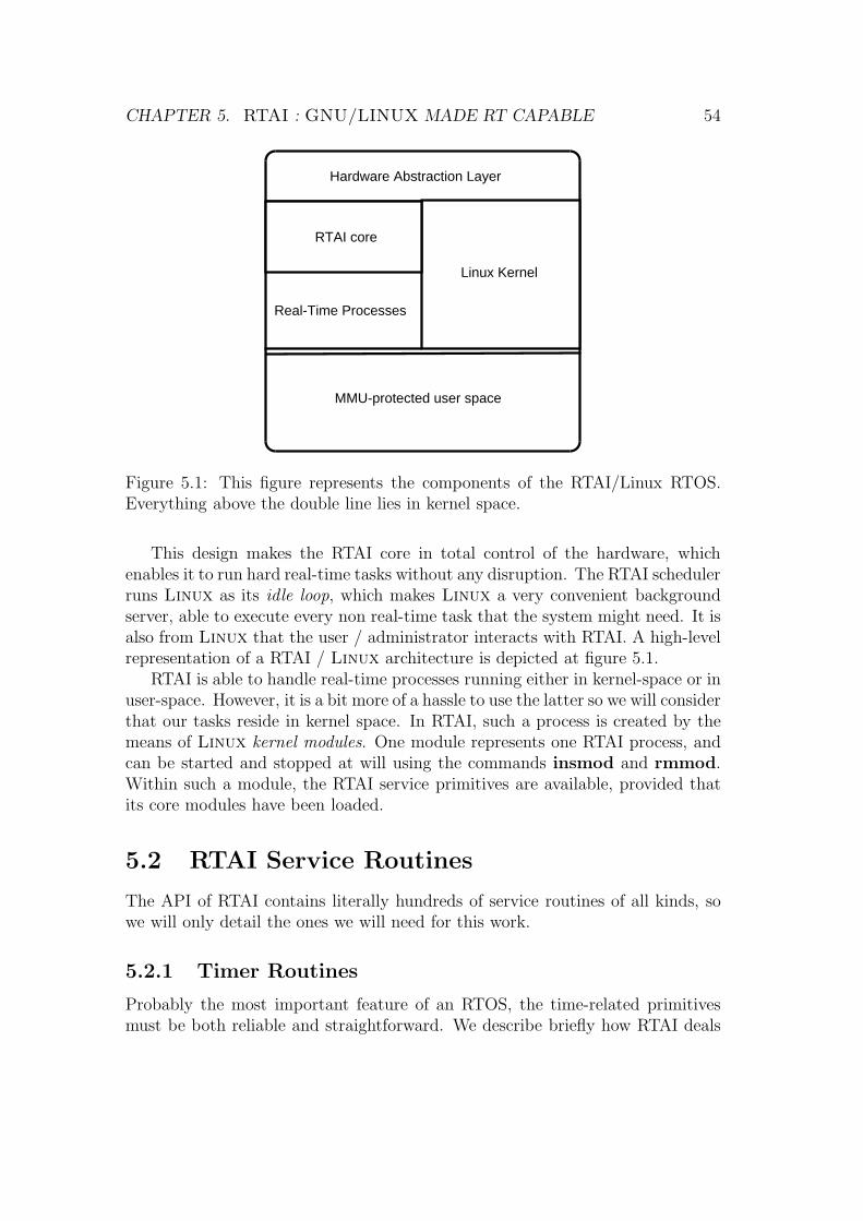
CHAPTER 5. RTAI : GNU/LINUX MADE RT CAPABLE 54
Hardware Abstraction Layer
RTAI core
MMU-protected user space
Linux Kernel
Real-Time Processes
Figure 5.1: This figure represents the components of the RTAI/Linux RTOS.Everything above the double line lies in kernel space.
This design makes the RTAI core in total control of the hardware, whichenables it to run hard real-time tasks without any disruption. The RTAI schedulerruns Linux as its idle loop, which makes Linux a very convenient backgroundserver, able to execute every non real-time task that the system might need. It isalso from Linux that the user / administrator interacts with RTAI. A high-levelrepresentation of a RTAI / Linux architecture is depicted at figure 5.1.
RTAI is able to handle real-time processes running either in kernel-space or inuser-space. However, it is a bit more of a hassle to use the latter so we will considerthat our tasks reside in kernel space. In RTAI, such a process is created by themeans of Linux kernel modules. One module represents one RTAI process, andcan be started and stopped at will using the commands insmod and rmmod.Within such a module, the RTAI service primitives are available, provided thatits core modules have been loaded.
5.2 RTAI Service Routines
The API of RTAI contains literally hundreds of service routines of all kinds, sowe will only detail the ones we will need for this work.
5.2.1 Timer Routines
Probably the most important feature of an RTOS, the time-related primitivesmust be both reliable and straightforward. We describe briefly how RTAI deals

CHAPTER 5. RTAI : GNU/LINUX MADE RT CAPABLE 55
with time readings.
One-shot and periodic modes
RTAI provides two different ways to get real-time class clock-readings : the one-shot and periodic modes. On Intel-based machines (we will not consider otherhardware platforms in this work but it should only differ slightly), both modesinteract with the 8254 Programmable Interval Timer (PIT) chip. This hardwarecounter can be programmed to :
• Trigger an interrupt after a certain amount of time has passed (this is usedby the one-shot mode).
• Trigger an interrupt at fixed periodic intervals (used by the periodic mode).
In the one-shot mode, the 8254 timer needs to be reprogrammed after eachinterrupt. This is very flexible (a different delay can be specified each time),but it generates a lot of overhead on low-end machines (reprogramming the PITtakes up a few CPU cycles). The periodic mode, however less flexible, has theadvantage of only needing to program the PIT once, and is hence less subjectto jitter. We will only use the periodic mode in the following, which is done inRTAI by calling the function rt_set_periodic_mode().
Clock-resolution setting
In the periodic mode, it is the interval between two clock interrupts which definesthe resolution of RTAI’s clocks. This is very convenient, because the 8254 PITaccepts a wide range of frequencies : from 1193180 Hz to about 18 Hz; we willthus bee able to choose the appropriate clock resolution. The PIT is programmedby writing a number of ticks in a 16-bit register. There are exactly 1193180 ticksin one second, thus writing the value 1 in the register makes the PIT triggerinterrupts at a frequency of a little more than a megahertz. This is obviously avery bad idea, because it is probably more interrupts than the CPU can handleand would ultimately lead to a crash1. The clock-resolution must hence be chosenwith care, by finding the best trade-off between interrupt-handling overhead andclock-precision.
To program the PIT in RTAI, simply call the function start_rt_timer(ticks).This call must be made after calling rt_set_periodic_mode(). Once the PITstarts triggering interrupts, the clocks of RTAI are updated automatically, andwe can start using them. When the timer is not needed anymore, it is advised tocall stop_rt_timer(), which reverts the PIT to its default settings.
1This was tried by the author on a 500 MHz Pentium machine, resulting as expected in acomplete freeze.

CHAPTER 5. RTAI : GNU/LINUX MADE RT CAPABLE 56
Reading the current time
Once the timer mode and clock-resolution have been set, we can start measuringtime by calling the primitive RTIME rt_get_time(). On all platforms, this callalways returns a 64-bit unsigned integer.
5.2.2 Task-Management Routines
The following describes how real-time tasks are created and managed in RTAI.
Creating a new task
RTAI holds all information about a task into a RT_TASK structure. A new taskis created using the rt_task_init function, which has the following signature :
int rt_task_init (RT_TASK *task,
void (*thread_main)(int),
int data,
int stack_size,
int priority,
int uses_fpu,
void(*signal)(void));
Calling this function initializes the task structure and creates a new taskwith the indicated parameters. The function pointer thread_main is the entrypoint of the task, and data is an integer that will be given as parameter tothread_main. The function signal will be called each time the scheduler setsthe task back in the running state, which enables the task to be aware thatit has been preempted (this parameter can be safely set to 0 if this feature isnot desired). The priority parameter must be an integer between 0 (highestpriority) and 255 (lowest priority). The RTAI scheduler does not require that alltasks have different priorities.
Making a task periodic
If we wish to create a periodic task, a subsequent call to the rt_task_make_periodicfunction must be made. Its signature is very straightforward :
int rt_task_make_periodic (RT_TASK *task,
RTIME offset,
RTIME period);
If task has been correctly initialized by rt_task_init, this call will make thetask periodic, with the specified offset and period values. Both offset andperiod are expressed in units defined by the clock resolution (set by start_rt_timer).

CHAPTER 5. RTAI : GNU/LINUX MADE RT CAPABLE 57
When the task is scheduled for the first time, its entry-point function is called.When the task returns from that function, it is stopped and will not be resched-uled. When a task is preempted, its context is saved, and will be restored whenrescheduled. A periodic task does not need to wait for preemption however, it canexplicitly yield its current period by calling the rt_task_wait_period() func-tion, which takes no parameters. The structure of a periodic task entry-pointfunction in RTAI would typically resemble the following :
void task_main (int data)
{
int running = 1;
while (running)
{
perform_important_things ();
if (are_we_done_yet ())
running = 0;
else
rt_task_wait_period ();
}
}
Deleting a task
Deleting unused tasks is needed so that the real-time scheduler does not fill upwith zombies2. This is done by simply calling rt_task_delete.
5.3 The RTAI Scheduler
To conclude this short presentation of RTAI, we briefly describe the RTAI sched-uler that will be used in the next chapter.
RTAI natively supports the use of 3 built-in schedulers : namely UP, SMPand MUP3. Only the first one is meant to be used on uni-processors machines (wewill not consider other cases in the following), so we shall use the UP scheduler.
As a standard fixed-priority scheduler, UP will always favor the pending taskwith highest priority (again, there are 256 unique priorities in RTAI, 0 being thehighest). The UP scheduler manages tasks with equal priorities by applying around-robin strategy. Priority assignments should hence be made using the RateMonotonic, or Deadline Monotonic algorithms.
2In Unix terminology, a zombie process is a process which has completed its execution butstill resides in the process table. While in this state, it is possible to investigate why the processwas terminated, and retrieve other useful information.
3UP, SMP and MUP respectively stand for “uni-processor”, “symmetric multi-processor”,and “multi uni-processor”.

CHAPTER 5. RTAI : GNU/LINUX MADE RT CAPABLE 58
In addition to the schedulers packaged with the RTAI distribution, RTAI alsoeasily supports custom-made schedulers. As every service in RTAI is materializedby kernel modules, using a custom scheduler amounts to simply load a differentmodule. This can be used for instance to implement a dynamic priority schedulerwith an Earliest Deadline First strategy.
Whichever scheduling strategy is used, this choice is orthogonal to our con-cerns. Remember that regarding scheduling, the only thing the Real-Time Se-mantics cares about is never to miss a deadline. How exactly this is guaranteedis beyond the scope of this work.
Chapter 6
Code Generation of Real-TimeControllers
In this chapter we present Spectre1, a tool for generating real-time code fromtimed-automata. Spectre currently generates code for RTAI but should beeasily adapted to work with any other RTOS. The following is divided in twomain parts : first we describe the tool’s input language and discuss the variousdesign choices which had to be made; in the second part, we describe how Spec-tre generates code and discuss the to which extent the generated code can beconsidered provably correct.
6.1 Input Language
The Spectre input language is composed of two sections :
1. The specification section describes the model of the controller in the formof a timed automaton.
2. The decoration section holds the controller’s functionality code. This sec-tion maps the timed automaton’s abstract behavior to concrete side-effects.
6.1.1 Specification Section
The syntax of this section is quite classic, as it is heavily inspired from theElastic input language [DDR05a], which is very similar to HyTech’s.
A short example of a Spectre specification can be found at figure 6.1. Thisexample really does nothing meaningful, it is only meant to present as manysyntactic elements as possible in a relatively short space. Most of the syntaxshould be rather self-explanatory, so we only explain the essential here. More
1Spectre stands for Specification de Controleurs Temps-Reels Embarques.
59

CHAPTER 6. CODE GENERATION OF REAL-TIME CONTROLLERS 60
specification example
clocks : x;
vars : a, b;
orders : o;
internals : i;
events : e;
initially A, {x := 0, a := 0, b := 0};
location A :
{x = 2, b = 1}, e, {a := 7}, B;
{3 <= x, x <= 4, b = 0}, e, {a := a + 4}, B;
{3 <= x, x <= 4, b = 1}, e, {a := a + 2}, B;
location B :
{a <= 10}, i, {a := a + 1}, B;
{a >= 10}, o, {a := 0, x := 0, b := 1}, A;
{a >= 10}, none, {a := 0, x := 0, b := 0}, A;
end
Figure 6.1: Example of a Spectre specification section.
information about the Spectre input language, along with a complete grammar,can be found in the appendix.
Comments on the specification syntax
The “initially” line indicates which location is the initial location of the automa-ton. The assignments on the right side of the line specify the initial values of theclocks and variables. There is a key difference here with HyTech for example,which specifies the initial clock and variables valuations with constraints ratherthan assignments, and thus allows non-deterministic initial valuations. As Spec-tre will ultimately need to generate code, it needs to know the precise initialvalue of each clock and variable. This should not be a problem in practice, ifa controller has been proven correct for a range of possible initial values, thedesigner can always choose precise values from that range.
Each “location” paragraph defines a location of the automaton and its out-going edges, if any. The syntax for edges is composed of (in that order) : guardpredicates, a label, updates, and the destination location. The guard predicates
CHAPTER 6. CODE GENERATION OF REAL-TIME CONTROLLERS 61
are separated by commas, and the guard as a whole is the conjunction of thepredicates it contains. Any empty guard is simply interpreted as True. The edgelabel can be either one of the previously declared events, orders or internals2, orthe keyword “none” which represents the silent label ǫ. Just like the initial valua-tions, the guards updates are expressed using a set of assignments. As expected,any unmentioned clock or variable is left untouched by the update.
A note about discrete variables
The perspicacious reader will have noted that, in the previous chapters, therewere no mention of discrete variables in the syntax of timed automata. Howdo these fit with the definition of timed automata given previously ? The an-swer is simple : discrete variables are just a very convenient syntactic additionto standard timed automata, which allows a designer to represent a timed au-tomaton in a more natural way. To translate a timed automaton with discretevariables into the “classical” syntax, just multiply every location by the numberof possible valuations of the discrete variables. As a direct consequence, for theautomaton to remain finite-state, there must be a finite number of possible valu-ations of the discrete variables. The usefulness of discrete variables in timed andhybrid automata is unquestioned in practice. The tools HyTech and Uppaalfor example, both allow their use extensively. A simple example showing how totransform a timed automaton with variables into its variable-less equivalent isshown at figure 6.2.
6.1.2 Decoration Section
As stated previously, the decoration section of a Spectre input file containsall the code and information necessary to produce a fully-functional real-timecontroller, that will be provably correct w.r.t to the specification3. The decorationis composed of several different items, which can be found at most once in thedecoration. We detail each item type in turn.
Global decoration
This item is optional, but it will most likely be present in any implementation. Itenables the user to provide global declarations. Everything that will be neededfurther on can be declared here -functions, global variables, includes, etc. Thefollowing code fragment shows how a global decoration item is declared in Spec-tre.
2The Elastic terminology identifies input labels as “events”, and output labels as “orders”.We have chosen to keep that terminology in Spectre.
3This will only hold under certain conditions which will be detailed later on.

CHAPTER 6. CODE GENERATION OF REAL-TIME CONTROLLERS 62
Figure 6.2: Transformation of a timed automaton with discrete variables into astandard timed automaton.
global
{%
#include "complex.h"
const int length = 8;
int var_a;
int array_b[length];
int b_index;
%}
Figure 6.3: Example of a Spectre global decoration item.
Variables decoration
Conceptually, the discrete variables are used in two different ways : in the guardpredicates they are read, and in the updates assignments they are written to. Foreach of those two uses, and for each variable, Spectre requires a code fragmentwhich will perform the read or write operation.
Short examples of reading and writing decoration items are shown in figure6.4. The items involving variable a are the simplest and probably the mostcommon use of this decoration. Other more sophisticated uses are possible, asshown by the decorations of b and c. Note that all identifiers (functions andvariables) mentioned in the decoration must be declared at the global level (seeabove).

CHAPTER 6. CODE GENERATION OF REAL-TIME CONTROLLERS 63
reading a {% return var_a; %}
writing a (val) {% var_a = val; %}
reading b {% return array_b[b_index]; %}
writing b (val) {% array_b[b_index] = val; %}
reading c {% return something_complex(); %}
writing c (val) {% update_the_complex_thing(val); %}
Figure 6.4: Example of Spectre reading and writing decoration items.
Labels decoration
Spectre takes a quite radical stance regarding labels, because it considers thatthey are somewhat context-free4. The tool is designed in such a way that theemission of an output or internal order will produce the same side-effects, regard-less of the source and destination locations of the edge to which the label wasattached. Likewise, an event label will be treated by the tool the same way inevery part of the automaton. While this radical choice may seem unnecessary atfirst, we believe that it will enforce cleaner and more elegant designs.
Order and internal labels require two code fragments, which we note d1 and d2.Upon crossing an edge from location A to location B labeled by σ, the producedcode will execute d1(σ) before the variables updates and d2(σ) after the updates.This enables the designer of a Spectre implementation to produce label side-effects which depend on the variable valuations in a fine-controlled manner. Asa result, labels in Spectre are not totally context-free, they can use a contextin the form of variable valuations.
Here is a small example of order and internal labels decoration. The keyword“nop” can be used to provide an explicitly empty code fragment.
internal i {% printf("before : a = %d", var_a); %}
{% printf("after : a = %d", var_a); %}
order o {% produce_some_side_effect(); %}
nop
Figure 6.5: Example of Spectre order and internal decoration items.
Event labels decoration items require three code fragments instead of two.This additional code fragment (which we note p(σ)) has the responsibility ofreturning a non-zero value if and only if there is an untreated occurrence of the
4This “context-freeness” is not absolute, as will be explained shortly.

CHAPTER 6. CODE GENERATION OF REAL-TIME CONTROLLERS 64
input label. The generated real-time task will call p(σ) every period, for everyevent label σ (that is, unless there is already an untreated occurrence of σ, inwhich case the function need not be called).
Here is an example of an event decoration in Spectre. The code fragmentsd1 and d2 were left empty, but this is of course not mandatory.
event e {% return event_e_has_arrived(); %}
nop
nop
Figure 6.6: Example of a Spectre event decoration item.
Transitions decoration
As with label decorations, the design choices behind Spectre’s way of decoratingtransitions might seem limiting at first glance. In Spectre, the implementationdesigner cannot associate a piece of code to a specific edge of the automaton.Rather, it is possible to attach code to the following events5 :
• The controller goes from location A to location B.
• The controller leaves location C.
• The controller enters location D.
• The controller makes a discrete jump, no matter which edge is used.
Just like with label decorations, it is possible to provide two code fragments foreach transition decoration item. As a consequence, it is possible to differentiateside-effects on a per-edge fashion to a limited extent. For instance, in the exampleof figure 6.1, there are two edges from B to A, and the code can tell which edgewas taken by testing the value of variable b after the updates have been computed.
The syntax for transitions decorations is straightforward, as illustrated by theexample of figure 6.7. The keyword “any” represents the set of all locations. Thisexample also illustrates Spectre’s comment syntax, which is borrowed from thelanguage Haskell, in which Spectre is written (line comments start with twoconsecutive minus symbols, and block comments are enclosed between “{-” and“-}”).
The “any to any” item would probably not be used in a production environ-ment but it is very useful for testing, by generating logs or execution traces forinstance.
5Here, event is meant in the broad sense, not as a type of label.

CHAPTER 6. CODE GENERATION OF REAL-TIME CONTROLLERS 65
A to B {% printf("going from A to B !"); %}
nop
any to B nop
{% printf("entering B !"); %}
A to any {% printf("leaving A !"); %}
nop
any to any {% printf("before update : i = %d", var_i); %}
{% printf("after update : i = %d", var_i); %}
B to B nop -- these two lines are,
nop -- as expected, useless
Figure 6.7: Example of Spectre transitions decoration items.
Restrictions
The Spectre input language uses restriction items in order to produce fully-deterministic implementations out of a non-deterministic model. Controller mod-els are usually non-deterministic because they represent the set of all possiblebehaviors of the controller, not its actual control flow. Restriction items providea way to specify the desired control flow precisely, without any modification tothe model.
Consider the following simple example. Both transitions are always enabled,because they represent a conditional statement that exclusively belongs to theimplementation. The two restriction items are used to provide this missing con-ditional statement.
{- ... -}
location A :
{}, none, {}, B;
{}, none, {}, C;
{- ... -}
restrict A to B {% return condition(); %}
restrict A to C {% return !condition(); %}
Figure 6.8: Example of Spectre restriction items.

CHAPTER 6. CODE GENERATION OF REAL-TIME CONTROLLERS 66
As with transitions decorations, it is not possible to restrict the crossing of anedge in particular. It is possible however, to use the keyword “any” in restrictions.
It should be noted that restriction items are dangerous if used poorly, becausethey can modify the controller’s behavior in such a way that correctness is nolonger assured. This issue will be treated more in depth later on in this chapter.
It is also worth noting that controller implementations do not need to be fully-deterministic. Some network protocols, for instance, take certain decisions atrandom. However, in that case, the implementation designer will need to providethe code which generates the random numbers and makes the appropriate choice.
Startup and cleanup decorations
These last two remaining decoration items are called just before the controllerstarts and right after it has completed its execution. It is useful for allocatingand freeing up resources, initializing variables, setting up peripherals, etc. Thesyntax for those items is straightforward, as shown by the following code excerpt.
startup {% /* allocate and initialize everything here */ %}
cleanup {% /* free up all used resources here */ %}
Figure 6.9: Spectre’s startup and cleanup decoration items.
6.2 Code Generation
In this section, we will first describe the code generation process, and then discussthe various conditions that need to be met in order to insure correctness.
6.2.1 Architecture of the Generated Code
The way Spectre works is quite straightforward, so we will not examine everydetail of the code generation process. Instead, we detail a number of key portionsof the generated code. Additional information can be found in the appendix,along with complete examples of Spectre’s output.
Additional defines
After running Spectre on an input file, the generated code needs a few smallmodifications before compiling. These modifications are however very limited, theimplementation designer only needs to encode the following numerical constants,which are defined in the first few lines of the generated file :
1. The period of the real-time task.

CHAPTER 6. CODE GENERATION OF REAL-TIME CONTROLLERS 67
2. The number of ticks between two clock interrupts.
3. The guard-enlargement constant.
4. The time unit, which maps the automaton time values to real time values.
5. The real-time task priority.
6. The real-time task stack size.
In code these constants are specified as pre-processor defines, as shown by thefollowing code fragment :
#define TIME_UNIT 7000
#define WIDENER 1001
#define PERIOD 1000
#define BEAT 11
#define STACK_SIZE 10000
#define TASK_PRIORITY 128 /* 0 = highest, 255 = lowest */
Figure 6.10: Pre-processor defines which need to be filled in before compiling.
The code of figure 6.10 specifies a clock interrupt frequency of one interruptevery 11 ticks. This makes for a clock resolution of 11
1193180seconds, which is
approximately 9,219061667 microseconds. With such a setting, the controllercan be safely verified using a ∆P of 10 microseconds. To distinguish the clock-resolution of the verification phase (∆P ) and the one that is used in code (whichcan be smaller), we use the term beat for the latter.
Setting the period define to 1000 specifies a period of 1000 beats, thus approx-imately 9,219061667 milliseconds. Since the Real-Time Semantics has the “fasteris better” property, such a setting could safely be guaranteed correct if the con-troller was verified with a ∆T of 10 milliseconds. Of course, the schedulabilityanalysis will need to be done using the real period value, not ∆T .
The widener define specifies a guard enlargement of 1001 beats. This is con-sistent with the definition of ∆S = ⌈∆T + ∆P ⌉∆P
.A time unit define of 7000 beats means that every numeric constant that is
compared or assigned to clocks in the automaton are multiples of 7000 beats. Forinstance, a guard testing the equality of a clock with the constant 3 in the automa-ton, will be true if that clock’s value lies in the interval [11×((3×7000)−1001)
1193180, 11×((3×7000)+1001)
1193180],
thus [0.184372014, 0.202828576], with both intervals being expressed in seconds.Finally, the remaining two defines are shown with their default values. They
need not be changed in normal circumstances, except maybe the task priority ifthere are other real-time tasks running on the target platform.

CHAPTER 6. CODE GENERATION OF REAL-TIME CONTROLLERS 68
Kernel module management and real-time main loop
Spectre’s output is the C source code of a Linux kernel module which, wheninserted into an RTAI-enabled kernel, launches a single periodic real-time task.The code of figure 6.11 shows how this is achieved in practice.
void spectre_task_main (int data) {
spectre_running = 1;
spectre_startup ();
spectre_transition_initially ();
while (spectre_running == 1) {
spectre_current_time = rt_get_time ();
spectre_check_for_events ();
spectre_current_location ();
rt_task_wait_period ();
}
spectre_cleanup ();
}
int spectre_init_module (void) {
rt_set_periodic_mode ();
start_rt_timer (BEAT);
rt_task_init (&spectre_task, spectre_task_main, 0, STACK_SIZE,
TASK_PRIORITY, USE_FPU, 0);
rt_task_make_periodic (&spectre_task, rt_get_time () + PERIOD, PERIOD);
return 0;
}
void spectre_exit_module (void) {
stop_rt_timer ();
rt_task_delete (&spectre_task);
}
module_init (spectre_init_module);
module_exit (spectre_exit_module);
Figure 6.11: Main loop and kernel module management routines.
The “init” and “exit” functions should be self-explanatory, all the RTAIprimitives used by Spectre were detailed in the previous chapter. The firstfunction of the figure is the entry point of the real-time task. Before enteringthe main loop, the startup decoration is called, followed by a call to the initialtransition. This call will initialize the clocks and variables and set the current

CHAPTER 6. CODE GENERATION OF REAL-TIME CONTROLLERS 69
location, all according to the “initially” line of the Spectre specification section.The current location is remembered by the code with a function pointer, whichis called every period (the internals of this function will be detailed further on).The loop body is consistent with the Real-Time Semantics : first the currenttime is read, then the inputs are checked, and finally the outgoing edges of thecurrent location are examined to see if any of them is enabled. This will result inat most one location change, before the current period is yielded. After the loopends, the cleanup decoration code is called and the real-time task stops.
Location functions
As stated just before, every location in a Spectre-generated controller is repre-sented by a function. This function, when called, examines every outgoing edgeof its location and fires the first enabled transition it sees. The generated codefor locations is extremely simple, as shown by figure 6.12.
void spectre_location_A (void)
{
if (spectre_check_A_to_B_1 ()) {
spectre_transition_A_to_B_1 (); return;
}
if (spectre_check_A_to_B_2 ()) {
spectre_transition_A_to_B_2 (); return;
}
}
Figure 6.12: Example of a location function.
Enabledness checking functions
For each edge of the automaton, Spectre generates a “check” function whichreturns a non-zero value if and only if its edge is currently enabled. This is done byevaluating the guard predicates, calling the appropriate restrictions decorations,and if necessary, verifying that there is an untreated occurrence of the attachedevent label.
The code in figure 6.13 shows an example of a check function. The functioncalls prefixed by “r” correspond to restrictions decorations. Every restrictionthat is not mentioned in the Spectre input file is given a function which simplyreturns 1. The internals of the “guard” function in the figure are describedhereafter.

CHAPTER 6. CODE GENERATION OF REAL-TIME CONTROLLERS 70
int spectre_check_A_to_B_1 (void) {
int spectre_r1, spectre_r2, spectre_r3, spectre_r4, spectre_g;
spectre_r1 = spectre_r_A_to_B ();
spectre_r2 = spectre_r_A_to_any ();
spectre_r3 = spectre_r_any_to_B ();
spectre_r4 = spectre_r_any_to_any ();
spectre_g = spectre_guard_A_to_B_1 ();
return (spectre_g && spectre_r1 && spectre_r2 &&
spectre_r3 && spectre_r4 && (spectre_e_is_pending == 1));
}
Figure 6.13: Example of a transition check function.
Guard evaluation functions
The code at figure 6.14 shows how the generated controller evaluates guards (inthis case, it is the guard {x = 2, p ≥ 7} with x being a clock and p a discretevariable). The spectre_equals function provides the enlargement mechanism.As mentioned in the beginning of this chapter, this guard evaluation functionuses the “read” decorations to retrieve the variable values.
int spectre_guard_One_to_Two_1 (void) {
RTIME spectre_t1, spectre_t2;
int spectre_e1, spectre_e2;
int spectre_res = 1, spectre_tmp;
spectre_t1 = spectre_read_x ();
spectre_t2 = (TIME_UNIT * 2);
spectre_tmp = spectre_equals (spectre_t1, spectre_t2);
spectre_res = spectre_tmp && spectre_res;
spectre_e1 = spectre_read_p ();
spectre_e2 = 7;
spectre_tmp = spectre_e1 >= spectre_e2;
spectre_res = spectre_tmp && spectre_res;
return spectre_res;
}
Figure 6.14: Example of a guard evaluation function.
Transitions functions
When a location function (described previously) detects an enabled edge, it callsthe corresponding “transition” function. This function calls the appropriate dec-

CHAPTER 6. CODE GENERATION OF REAL-TIME CONTROLLERS 71
orations, computes the clocks and variables updates, and updates the currentlocation appropriately. An example of such a function is illustrated at figure6.15.
void spectre_transition_A_to_B_1 (void)
{
spectre_d1_A_to_B ();
spectre_d1_A_to_any ();
spectre_d1_any_to_B ();
spectre_d1_any_to_any ();
spectre_d1_e ();
spectre_update_A_to_B_1 ();
spectre_current_location = spectre_location_B;
spectre_d2_e ();
spectre_e_is_pending = 0;
spectre_d2_A_to_B ();
spectre_d2_A_to_any ();
spectre_d2_any_to_B ();
spectre_d2_any_to_any ();
}
Figure 6.15: Example of a transition function.
The transition function first calls the d1 transition decorations. Any suchdecoration that was not present in the input file is replaced by an empty stub(this also applies to “nop” fragments). Right after, the d1 label decoration iscalled, followed by the clocks and variables updates, the location update, the d2
label decoration, and the reset of the event label pending flag (this last action isonly performed for event labels, obviously). Finally, the d2 transitions decorationsare called.
These numerous function calls might raise some performance concerns. How-ever, we believe that this should easily be solved if a good optimizing compiler isused, which will “inline”6 many (if not all) of these calls, and simply remove theempty stubs.
Updates functions
Updates functions are called by the transitions functions to perform the clocksand variables updates. It uses both the “read” and “write” decorations to perform
6“Inlining” is a common optimization trick which replaces a function call by a copy of thatfunction’s body. This generates faster code (the call / return sequence is saved), at the cost ofa larger executable.

CHAPTER 6. CODE GENERATION OF REAL-TIME CONTROLLERS 72
the updates. The example of figure 6.16 shows the generated update function forthe assignments {x := 2, a := a + 4}.
void spectre_update_A_to_B_2 (void)
{
spectre_write_x (TIME_UNIT * 2);
spectre_write_a (spectre_read_a () + 4);
}
Figure 6.16: Example of an update function.
6.2.2 Correctness of the Generated Code
In the following, we shall not prove that the code generated by Spectre iscorrect, as that would require a very involved effort that is beyond the scope ofthis work. Rather, we will enumerate a number of necessary conditions that needto be met to insure correctness, and then give informal arguments showing thatthese conditions should be sufficient in practice.
Necessary conditions for correctness
In the following, we will assume that the AASAP semantics of the automatongiven in the specification has been proven to satisfy a set of safety properties, forsome positive value ∆. We will assume that the designer assigned values to theReal-Time Semantics parameters such that the inequality ∆ > ∆T +2∆D+4∆P issatisfied. The generated code needs to satisfy the following requirements (detailsfollow) :
(R1) The clock resolution set by the BEAT define must not be greater than ∆P .
(R2) The PERIOD define must not be greater than ∆T .
(R3) The WCRT of the task loop must not be greater than ∆D.
(R4) All decorations code fragments must be proven free of run-time errors.
(R5) All decorations code fragments must be proven to terminate.
(R6) The WIDENER define must be set to PERIOD + 1.
(R7) The restrictions decorations must only reduce non-determinism.
(R8) The input-checking functions must be proven never to miss any event.
(R9) The PRIORITY define must be set such that the task is proven schedulable.

CHAPTER 6. CODE GENERATION OF REAL-TIME CONTROLLERS 73
The requirements (R1) through (R3) are very natural. If the real-time seman-tics inequality holds for a set of parameters, it will remain true if the parameterseffectively used are smaller.
The requirements (R4) and (R5) are related to requirement (R3). The gen-erated code must be proven to always complete a task loop without errors andwithin the deadline. Proving this in a formal way requires techniques which arebeyond the scope of this work. However, if great care is put into the decorationprogramming, it might suffice in practice.
Requirement (R6) comes from the definition of ∆S = ⌈∆T + ∆P ⌉∆P.
Requirement (R7) insures that the generated controller’s behavior is somehowa refined version of the original automaton. It is easy to prove that reducing non-determinism does not break safety-properties7.
Requirement (R8) needs to be met because we made the hypothesis that thecontroller was input-enabled. For this hypothesis to hold in practice, we need tomake sure that the input-polling functions never miss an event.
Requirement (R9) comes from the Real-Time Semantics, which makes thehypothesis that the deadline is always met.
Final notes on code correctness
Because it follows precisely the strategy dictated by the Real-Time Semantics,the code generated by Spectre (without the decorations) can be consideredcorrect by construction. Moreover, if great care has been put in the decorationeffort, and if all the requirements just described are proven to be satisfied, then itseems reasonable to have great confidence in the generated controller, decorationsincluded.
6.3 Use of the Spectre Decoration Language
The decoration language of Spectre is simple and straightforward but to someextent somewhat limiting. Indeed, for an arbitrary controller automaton, a Spec-tre decoration file might be hard to write (because of the impossibility to deco-rate an edge in particular for instance). However, if is known during the modelingphase that Spectre will be used for code generation, we believe that it shouldbe rather simple to deal with its few limitations. Here are two guidelines to followwhen modeling a controller to use with Spectre :
• The semantic weight should be stressed on locations. Going from a locationA to a location B should have a meaning that is independent of the edgefollowed.
7This is because the existence of a simulation relation is easy to show.

CHAPTER 6. CODE GENERATION OF REAL-TIME CONTROLLERS 74
• Synchronization labels should have a meaning of their own, regardless ofwhere they are used in the automaton.
Clearly, these guidelines seem reasonable for an automaton that is intendedto be used for code generation.
6.4 Implementation of Spectre
The current Spectre implementation is made of about 3000 lines of Haskell8.The parsing code was created using the Alex lexical analyzer generator, and theHappy parser generator. The rest of the Spectre source code is composed of asemantic checker and the code generator itself. The entire source code is freelyavailable upon request to the author : [email protected]
As Haskell is completely portable, Spectre should run without modificationon any platform.
8Haskell is a purely functional language. Compilers, interpreters and documentation forHaskell are available at http://www.haskell.org

Chapter 7
Case Study : Philips AudioControl Protocol
This chapter illustrates how our methodology is used in practice, from verificationto code generation. For this purpose, we have chosen to implement a simplereal-time data transmission protocol, namely the Philips Audio Control Protocol(PACP in the following). This physical-layer protocol was designed by Philipsengineers for stereo device equipments, and uses Manchester encoding to sendarbitrary long binary sequences on a wire between a single sender and a receiver.We have chosen to implement this particular protocol for the following reasons :
1. Because it is a physical-layer protocol using Manchester encoding, a soft-ware implementation must run on a real-time platform to insure correctness.
2. The protocol has already been analyzed with the Almost ASAP semanticsin [DDR05a], so we will use their verification results.
3. The protocol is quite subtle, and is arguably difficult to implement by hand.This advocates in favor of code generation.
4. The experimental setup needed for implementation and testing is very lim-ited : only a single low-cost PC is required. Optionally, one could also linktwo machines with a single cable.
The following is structured as follows : first we describe the data transmissionprotocol informally, then we present the modeling effort and verification resultsobtained in [DDR05a], and finally we describe the implementation process usingthe tool Spectre.
Remark : Figures 7.4 through 7.7 are found at the end of this chapter.
75

CHAPTER 7. CASE STUDY : PHILIPS AUDIO CONTROL PROTOCOL 76
7.1 Description of the PACP
As stated just above, the protocol uses Manchester encoding to transmit binarysequences. The binary information is sent by changing the wire voltage in themiddle of evenly-spaced time slots. Each time slot holds one bit of information;if the voltage goes from a low state to a high state in the middle of the timeslot then a “1” is transmitted. If on the contrary, the switch went from high tolow voltage then it is considered by the receiver as a “0”. The PACP faces thefollowing difficulties :
• Even if the sender and receiver agree on the length of a time slot, they runasynchronously so they do not know where the time slot begins.
• The protocol needs to work for binary sequences of any length, so thereceiver needs a way of detecting the beginning and end of a sequence.
• The receiver cannot detect voltage switches from high to low reliably1
(called DOWN signals from now on), so it will need to rely solely on switchesfrom low to high (UP signals).
The above issues are solved by the PACP as follows : when no transmissiontakes places, the wire voltage stays low. To initiate a sequence, the sender startsby sending an UP signal, which is understood by the receiver as the middle of thefirst time-slot. The binary sequence is then sent using the standard Manchesterencoding technique. To decode the binary sequence, the receiver simply measuresthe time elapsed between consecutive UP signals. This works fine except for theend of the sequence, because by relying only on UP signals, the receiver cannotdistinguish sequences ending with “1” from those ending with “10”. This isillustrated at figure 7.1.
As seen in the figure, the difference between “111” and “1110” is marked onlyby the time of the last DOWN signal, which the receiver does not see. The PACPsolves this problem by requiring that all transmitted sequences be either odd inlength or end with “00”.
7.2 Modeling the PACP with Timed Automata
In [DDR05a], Raskin et al. have analyzed the PACP using the Almost ASAPsemantics. The purpose of the article was to illustrate the practical and theoreti-cal attractiveness of the Almost ASAP semantics compared to other approaches,which do not address the synchrony hypothesis thoroughly. They also brieflydescribed a code generation scheme which targets the Lego Mindstormstm
platform, but the emphasis was clearly on the more theoretical aspects.
1This limitation comes from the original target hardware environment of the PACP.

CHAPTER 7. CASE STUDY : PHILIPS AUDIO CONTROL PROTOCOL 77
-
-
1 1 1
1 1 1
0 t
t
V
V
Figure 7.1: Manchester encodings for sequences “111” and “1110”.
As our work focuses on code generation, rather than model-checking, we re-view the verification results obtained in [DDR05a], but without much detail asto how they were obtained. The interested reader will find this information in[DDR05a].
7.2.1 Sender Automaton
A timed automaton for the PACP sender controller is depicted at figure 7.2. Ithas a single clock x, and three discrete variables p, dz and i. Again, these discretevariables could have been encoded in the locations, but this has not been donefor the sake of clarity. These variables have the following meaning :
• p is used to remember the parity of the transmitted sequence (0 for even, 1for odd).
• dz (standing for “double zero”) contains 1 if the last two transmitted bitswere “00”, and 0 otherwise.
• i contains the next bit to be transmitted, and is read by the sender toproduce UP and DOWN signals appropriately. During verification, thisvariable is assigned to a non-deterministic binary value, which can changeat any time.
As the first UP signal does not correspond to a transmitted bit, the sequenceparity is initialized to 0. Every time a bit is sent, the update p := 1-p sets thenew parity appropriately. When the automaton goes from WaitZero to ZeroSent,we know we have just sent two consecutive zeroes, variable dz is thus set to 1.
Observe that the sender automaton non-deterministically chooses to end orcontinue to transmit, after sending each bit. This makes the sender automatonvalid for any binary sequence of finite length.

CHAPTER 7. CASE STUDY : PHILIPS AUDIO CONTROL PROTOCOL 78
Figure 7.2: Sender automaton for the PACP.
Finally, the predicate {x ≥ 12} attached to the edge from Idle to OneSent isthere to ensure that the sender stays idle for at least three time slots between twoconsecutive sequences. This is necessary because the receiver automaton relieson that period of inactivity to detect the end of the sequence.
7.2.2 Receiver Automaton
The receiver automaton is a bit more simple because it has only three location,and it is illustrated at figure 7.3. It has one clock y and two discrete variablesm and r. The m variable is equivalent to the p variable of the sender automatonand contains the parity of the received sequence. The receiver uses this variableto determine whether it needs to append a final “0” to the binary stream whenthe transmission ends. Variable r is assigned to the received bit(s) each time thereceiver sees an UP signal (except the for the first UP signal). When r is assignedthe value 2, it means that the receiver has decoded “01”.
Each time the automaton sees an UP signal, it rounds the reception timeto the closest time-slot center. This is what makes the PACP robust : if allaccumulated clock-rounding errors never reach more than one quarter of a time-

CHAPTER 7. CASE STUDY : PHILIPS AUDIO CONTROL PROTOCOL 79
Figure 7.3: Receiver automaton for the PACP.
slot, then the receiver will be able to decode each UP signal appropriately. TheAlmost ASAP semantics enables us to prove this in a formal fashion.
7.3 Verification Results
In [DDR05a], it is shown that the above specification is correct in the context ofthe Almost ASAP semantics iff the sum of the respective ∆ parameters of thesender and receiver automata is strictly less than one sixteenth of a time slot.Formally, for an appropriate Observer automaton, and U being one quarter of atime-slot :
Reach([[Sender]]AAsap∆1
|| [[Receiver]]AAsap∆2
|| [[Observer]])∩Bad = φ iff ∆1 + ∆2 <1
4U
We see from the above formula that the ∆ parameters of the automata arerelated : if one controller is less precise (i.e. has a higher ∆ parameter), theother must compensate to retain correctness of the whole (by decreasing its ∆

CHAPTER 7. CASE STUDY : PHILIPS AUDIO CONTROL PROTOCOL 80
parameter). If the hardware platforms of both controllers are equal then thebest throughput (which is directly related to U , the length of a time-slot) will beobtained by assigning both ∆ parameters to the same value.
7.4 Systematic Implementation of the PACP
using Spectre
Now that we have given a complete specification of the PACP and indicated underwhich conditions it is proven correct, we can describe how the implementationprocess is achieved.
7.4.1 Sender Specification
The Spectre specification section of the PACP sender controller is given at figure7.4. This section should be straightforward, as it is simply a textual version ofthe automaton of figure 7.2.
7.4.2 Sender Decoration
A Spectre decoration section for the sender automaton is found at figure 7.5.We comment each decoration item in turn.
Global decoration
This implementation of the PACP uses the parallel port to transmit data. Onour target platform (a Intel-based PC), sending data through the parallel port isachieved by writing a byte at the memory address 0x378. The parallel port canbe configured in various modes, which is done by writing the appropriate byte atthe memory address 0x37A.
Variables var_p and var_dz will be used to store their respective automatonvariables. For the i variable, it is a bit more complicated as we do not wantour controller to send random bits. Instead, we declare an array data[] alongwith an index, and we will map the i variable to the contents of data[] at indexdata_index.
Finally, we declare a small boolean function : sequence_finished(), whichwill be used to make the implementation deterministic.
Labels decorations
The UP order of the sender automaton is decorated by a single call to the outb
function, which sets all data bits of the parallel port to 1. Similarly, the decorationfor the DOWN order clears all bits of the parallel port back to 0.

CHAPTER 7. CASE STUDY : PHILIPS AUDIO CONTROL PROTOCOL 81
Startup and cleanup decorations
The only initializations that the sender needs to perform are (1) configure theparallel port for output, and (2) put the initial data bits to 0. No cleanupdecoration is needed.
Variables decorations
The decorations for variables p and dz are straightforward. Variable i is boundto the next bit to be sent, thus data[data_index]. The array-accessing code isprotected by a conditional statement ensuring that we will never access the wrongmemory space. As our controller runs in kernel mode and is thus not subject topage fault violations, this might seem unnecessary. We do it anyway for the sakeof best practices.
Transitions decorations
The transitions decorations are used to initialize and increment the data indexwhen necessary. When the automaton goes from Idle to OneSent, we know thatthe transmission starts so we take this opportunity to initialize data_index to0. When entering OneSent from locations WaitOne and ZeroSent, we know wehave just sent a “1” bit so we increment data_index. Similarly, when enteringlocation ZeroSent from anywhere, we know that a “0” has been sent so weincrement data_index in this case as well.
Finally, when the automaton goes back to Idle, we know that the transmis-sion is complete so we set the spectre_running flag to 0. This will cause thereal-time task to stop.
Restrictions
The final part of the decoration section uses five restrictions to make the sendercontroller fully-deterministic. The non-determinism of the sender automatoncomes from the fact that it can go back to Idle, and thus end the transmission,after each bit is sent. Hence, to make the sender controller deterministic we mustmake sure that the two following statements are true :
1. The controller does not end the transmission until it is finished.
2. The controller does end the transmission when it is finished.
This can be expressed in Spectre by using the following restrictions :
1. restrict any to Idle {% return sequence_finished(); %}
CHAPTER 7. CASE STUDY : PHILIPS AUDIO CONTROL PROTOCOL 82
2. restrict any to WaitZero {% return !sequence_finished(); %}
restrict any to WaitOne {% return !sequence_finished(); %}
restrict any to ZeroSent {% return !sequence_finished(); %}
restrict ZeroSent to OneSent {% return !sequence_finished(); %}
It is easy to see that the above restrictions have the effect of only reducingnon-determinism.
7.4.3 Receiver Specification
The Spectre specification section for the PACP receiver controller can be foundat figure 7.6. Again, this is simply a textual representation of the receiver au-tomaton given earlier in this chapter. Notice the usage of the “none” keyword,which represents the silent label.
7.4.4 Receiver Decoration
A Spectre decoration section for the receiver automaton can be found at figure7.7. We comment each decoration item in turn.
Global decoration
The global decoration of the PACP receiver controller is very similar to thesender’s. The GOOD_INDEX define is slightly modified (it requires data_index
to be at least two positions away from the bottom of data[]) because the re-ceiver will write up to two bits at once in the data[] array. As the data[] arrayis statically allocated with a length of 128, this implementation of the PACPreceiver only supports transmission of up to 128 bits2.
Labels decorations
The only label of the receiver automaton is the input UP signal. In the Spectreinput file, we must decorate this event with a function which returns a non-zerovalue if and only if an untreated occurrence of UP is detected. To achieve this,the receiver controller reads the contents of the parallel port data register everyperiod (stored in val), and remembers the value read at the previous period ina global variable last_val. The following table shows the various possibilities.A “1” in the table represents a non-zero value.
2It might seem silly to waste a whole integer (four bytes on our target platform) to storeone bit of information. This is done solely to alleviate the figures.

CHAPTER 7. CASE STUDY : PHILIPS AUDIO CONTROL PROTOCOL 83
last_val val event up
0 0 00 1 11 0 01 1 0
Admittedly, this way of checking for the UP signal is a bit cheating, becauseit relies on seeing the DOWN signals reliably (third line in the table). We couldhave avoided cheating by providing a handler for the parallel port interrupt line(IRQ 7 on Intel-based machines), but we have chosen not to do so to keep thereceiver decoration short and simple.
It is easy to see that this input-polling function will never miss an event. Sincewe have that ∆ < 1
8U and ∆ > ∆T +2∆D +4∆P , we know that the period of the
real-time task will be at least 32 times smaller than the time-slot. It should hencebe impossible for the controller to miss an event by using this polling function.
Startup and cleanup decorations
The startup decoration configures the parallel port for input use, and initializesthe variables that are not initialized by the initially line of the specification.
The cleanup decoration simply prints out the received bits to the kernel log.This output can be consulted in Linux by using the dmesg command, or byreading the file /var/log/messages.
Variables decorations
The decoration of variable m is straightforward. Remember that the r variable iswritten by the receiver automaton when it has decoded a new bit (or sometimestwo consecutive bits). Hence, we provide a writing decoration for that variable,which writes to the data[] array whatever r is written to. Again, the arrayaccessing code is protected by a conditional statement. If the sender goes madand sends more than what the receiver can handle, we need to make sure thatno buffer overflow will occur. This is especially important because the receivercontroller runs in kernel space, where memory corruption is very destructive tosay the least.
Transitions decorations
The only transition decoration of the receiver is one that makes the controllerstop when the sequence is finished (i.e. when the automaton goes back to Idle).

CHAPTER 7. CASE STUDY : PHILIPS AUDIO CONTROL PROTOCOL 84
7.4.5 Assigning the RT Semantics Parameters
One last step is needed before our implementation of the PACP is complete.After running each input file through the Spectre tool, we need to encode somenumerical constants in the BEAT, PERIOD, WIDENER and TIME_UNIT defines. Toensure correctness, we must respect the following equations :
∆ > ∆T + 2∆D + 4∆P
U > 8 × ∆
U < (1193180)−1 × BEAT× TIME_UNIT
∆T > (1193180)−1 × BEAT× PERIOD
∆P > (1193180)−1 × BEAT
∆D > WCRT of the task
WIDENER = PERIOD + 1
On our testing machines, a safe setting for the clock resolution is 11 ticks.Also, some very approximate WCET analysis shows that both the sender andreceiver controllers will always be able to complete a task loop within a timecertainly not larger than 1 millisecond. As a CPU usage of 50% seems sufficientlyhigh, we set the period to 2 milliseconds. These observations suffice to assign asafe value to the remaining parameters, which we do as follows :
BEAT = 11 → ∆P = 10 µs
∆P = 10 µs
∆D = 1 ms
∆T = 2 ms → ∆ = 5 ms
∆ = 5 ms → U = 45 ms
U = 45 ms → TIME_UNIT = 5000
∆T = 2 ms → PERIOD = 200
PERIOD = 200 → WIDENER = 201
7.5 Execution of the Generated Code
The generated code has been successfully tested on two 500MHz Pentium ma-chines. With the above settings, the actual CPU usage observed in practice isless than 1%. This shows that our WCET analysis was very pessimistic indeed.More fine-grained WCET and schedulability analysis could be used to push thethroughput to several hundred bits per second (with the above settings it is alittle over 5 bits per second). Peformance-wise, this seems very satisfying consid-ering that (1) everything is done in software, (2) this software is provably correct,and (3) the hardware used is quite modest.
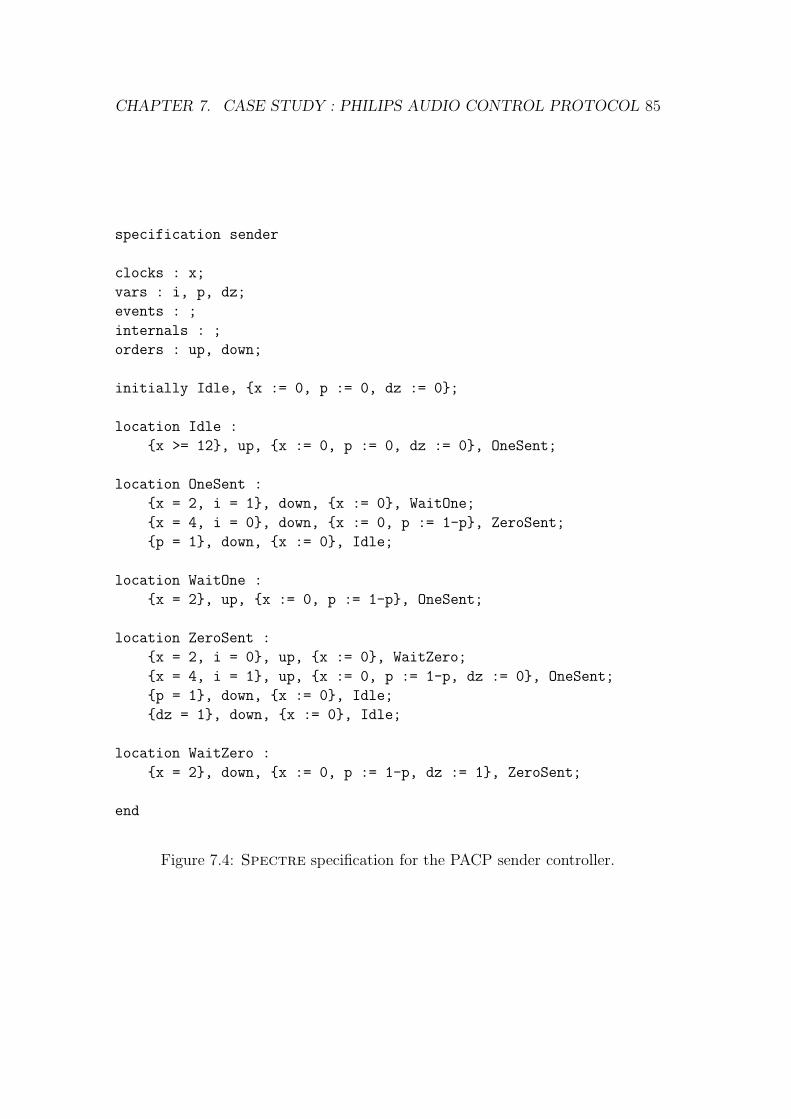
CHAPTER 7. CASE STUDY : PHILIPS AUDIO CONTROL PROTOCOL 85
specification sender
clocks : x;
vars : i, p, dz;
events : ;
internals : ;
orders : up, down;
initially Idle, {x := 0, p := 0, dz := 0};
location Idle :
{x >= 12}, up, {x := 0, p := 0, dz := 0}, OneSent;
location OneSent :
{x = 2, i = 1}, down, {x := 0}, WaitOne;
{x = 4, i = 0}, down, {x := 0, p := 1-p}, ZeroSent;
{p = 1}, down, {x := 0}, Idle;
location WaitOne :
{x = 2}, up, {x := 0, p := 1-p}, OneSent;
location ZeroSent :
{x = 2, i = 0}, up, {x := 0}, WaitZero;
{x = 4, i = 1}, up, {x := 0, p := 1-p, dz := 0}, OneSent;
{p = 1}, down, {x := 0}, Idle;
{dz = 1}, down, {x := 0}, Idle;
location WaitZero :
{x = 2}, down, {x := 0, p := 1-p, dz := 1}, ZeroSent;
end
Figure 7.4: Spectre specification for the PACP sender controller.

CHAPTER 7. CASE STUDY : PHILIPS AUDIO CONTROL PROTOCOL 86
decoration sender
global
{%
#define DATA_REGISTER 0x378
#define CTRL_REGISTER 0x37A
#define GOOD_INDEX (0 <= data_index && data_index < data_length)
int var_p, var_dz, data_index;
int data[] =
{ 1, 1, 1, 1, 1, 1, 1, 1, 1, 0, 1, 0, 1, 0, 1, 1,
1, 0, 1, 0, 1, 1, 1, 1, 1, 0, 1, 0, 1, 0, 1, 1,
1, 0, 1, 1, 1, 0, 1, 1, 1, 0, 1, 0, 1, 0, 1, 1,
1, 1, 1, 0, 1, 0, 1, 1, 1, 1, 1, 1, 1, 1, 1, 1, 0, 0
};
const int data_length = 8*8+2;
int sequence_finished(void) {return data_index >= data_length;}
%}
order up {% outb(255, DATA_REGISTER); %} nop
order down {% outb(0, DATA_REGISTER); %} nop
startup {% outb(0, CTRL_REGISTER); outb(0, DATA_REGISTER); %}
cleanup nop
reading i {% return GOOD_INDEX ? data[data_index] : 0; %}
reading p {% return var_p; %}
writing p (value) {% var_p = value; %}
reading dz {% return var_dz; %}
writing dz (value) {% var_dz = value; %}
Idle to OneSent {% data_index = 0; %} nop
WaitOne to OneSent {% data_index++; %} nop
ZeroSent to OneSent {% data_index++; %} nop
any to ZeroSent {% data_index++; %} nop
any to Idle {% spectre_running = 0; %} nop
restrict any to Idle {% return sequence_finished(); %}
restrict any to WaitZero {% return !sequence_finished(); %}
restrict any to WaitOne {% return !sequence_finished(); %}
restrict any to ZeroSent {% return !sequence_finished(); %}
restrict ZeroSent to OneSent {% return !sequence_finished(); %}
end
Figure 7.5: Spectre decoration for the PACP sender controller.

CHAPTER 7. CASE STUDY : PHILIPS AUDIO CONTROL PROTOCOL 87
specification receiver
clocks : y;
vars : m, r;
events : up;
internals : ;
orders : ;
initially Idle, {y := 0, m := 0};
location Idle :
{}, up, {y := 0, m := 0}, LastIsOne;
location LastIsOne :
{3 <= y, y <= 5}, up, {y := 0, m := 1-m, r := 1}, LastIsOne;
{7 <= y}, up, {y := 0, r := 2}, LastIsOne;
{5 <= y, y <= 7}, up, {y := 0, m := 1-m, r := 0}, LastIsZero;
{9 <= y, m = 0}, none, {r := 0}, Idle;
{9 <= y, m = 1}, none, {}, Idle;
location LastIsZero :
{3 <= y, y <= 5}, up, {y := 0, m := 1-m, r := 0}, LastIsZero;
{5 <= y, y <= 7}, up, {y := 0,r := 2}, LastIsOne;
{7 <= y}, none, {r := 0}, Idle;
end
Figure 7.6: Spectre specification for the PACP receiver controller.

CHAPTER 7. CASE STUDY : PHILIPS AUDIO CONTROL PROTOCOL 88
decoration receiver
global
{%
#define DATA_REGISTER 0x378
#define CTRL_REGISTER 0x37A
#define GOOD_INDEX (0 <= data_index && data_index < data_length-1)
const int data_length = 128;
int var_m, data_index, data[data_length];
unsigned char last_val;
void print_received_bits(void) {
int i;
if(GOOD_INDEX)
for(i = 0; i < data_index-1; i++) rt_printk("%d\n", data[i]);
else
rt_printk("ERROR : received more bits than buffer length...\n");
}
%}
event up
{%
unsigned char val = inb(DATA_REGISTER);
return val == last_val ? 0 : (last_val = val);
%} nop nop
startup {% outb(32, CTRL_REGISTER); last_val = 0; data_index = 0; %}
cleanup {% print_received_bits(); %}
reading m {% return var_m; %}
writing m (val) {% var_m = val; %}
writing r (val)
{%
if(!GOOD_INDEX) return;
switch (val) {
case 0: case 1: data[data_index++] = val; break;
case 2: data[data_index++] = 0; data[data_index++] = 1;
}
%}
any to Idle {% spectre_running = 0; %} nop
end
Figure 7.7: Spectre decoration for the PACP receiver controller.

Chapter 8
Conclusions
The objective of this work was to develop a methodology for creating provablycorrect software systematically, in the context of real-time embedded controllers.A controller in our context is a software-operated device which interacts witha physical environment and has the responsibility of keeping that environmentin a safe configuration. Our methodology belongs to the so-called “top-down”approach to the creation of provably correct software, which can be summarizedas follows : first, a formal model for the system (controller and environment)is created; second, a formal property is specified; third, the model is checked(usually with automated tools) against the property; and finally, the controlsoftware is constructed systematically and is guaranteed correct by construction.
In this work, we have put a lot of effort into ensuring that the models we useare realistic in the sense that they do take into account the software and hardwarelimitations that a real-time controller implementation must face. Indeed, manyverification approaches to this day make a number of simplifications regardingthese limitations, by making the hypothesis that no computation delay or datatransmission delay will ever be large enough to cause any harm. This can bejustified informally in a number of cases, but clearly there are situations wherethose simplifications need to be formally validated. To this end, we have usedrecent research from Raskin et al. [DDR05b] which proposes an elegant way ofdealing with these simplifications formally, namely the Almost ASAP Semantics.
Experimental testing has revealed that the code generated using the AlmostASAP Semantics approach, when run on a hard real-time platform, behavesbetter than expected. These experimental results suggested that the model forthe control software was somehow too coarse than needed, and that it hencecould be refined. Further investigation revealed the possibility to perform thisrefinement by making a few assumptions about the run-time environment, namelythe presence of a hard real-time operating system. This has led to the creationof a new implementation semantics, which we named Real-Time Semantics, thatprovides a tighter model for the control software. To validate this new semantics,we have constructed a simulation proof with the Almost ASAP Semantics, which
89

CHAPTER 8. CONCLUSIONS 90
resulted in a non-trivial adaptation of a similar proof found in [DDR05b].As our work was focused more on code generation than on model-checking, we
have only illustrated the use of safety properties, which require the environmentto avoid a subset region of its state-space. Our methodology could be used withmore complex specifications however, such as LTL formulas.
The final part of our work has been to develop a code generator which wasmeant to illustrate the practical applicability of our approach. This step involvedthe design of an input language composed of two parts called specification anddecoration. The former is used to encode the controller’s timed automaton andis very classic, borrowing heavily from the syntax of the tools HyTech andElastic. The decoration part of the language has been developed from theground up however, and much effort has been put into making it as generic andstraightforward as possible. The final result is a trade-off between simplicityand expressive power. Much of the involved design choices were made in favor ofstraightforwardness, which we believe is especially important since the decorationprogramming effort is the only part of our methodology which is not formallyensured correct. Hence, a simple and effective tool with some limitations seemedmore appropriate than one more powerful but intricate and harder to manipulate.
The code generation process itself that we have implemented has also beendesigned with straightforwardness in mind. This makes it easier to be convincedthat the generated code follows the Real-Time Semantics very closely, and canhence be considered correct by construction. This correctness is only ensuredwithin a certain set of requirements however, which we have tried to enumeratein the most exhaustive way possible.
As final note, it is interesting to point out that the case study we have pre-sented in the previous chapter is a fine example of what could barely be possibleto verify only ten years ago. In contrast, the model-checking tools available todayare able to perform this verification in a matter of seconds, and that is by usingthe Almost ASAP Semantics which is much coarser than the classical semanticsand is thus harder to verify. This clearly illustrates the progress made in the fieldin recent years, and without which this work would not have been possible.

Appendix A
Spectre Grammar
A.1 Typographical Conventions Used
Empty symbol : ǫNon terminals : 〈non terminal〉Keyword terminals : keyword_terminal
Non keyword terminals : non keyword terminal
A.2 Grammar
〈spectre input〉 :: 〈specification〉〈decoration〉
〈specification〉 :: specification
identifier
〈declarations〉〈initially〉〈locations〉end
〈declarations〉 :: ǫ| 〈declaration〉
〈declarations〉
〈declaration〉 :: 〈clocks declaration〉| 〈vars declaration〉| 〈events declaration〉| 〈orders declaration〉| 〈internals declaration〉
91

APPENDIX A. SPECTRE GRAMMAR 92
〈clocks declaration〉 :: clocks : 〈identifier list〉 ;〈vars declaration〉 :: vars : 〈identifier list〉 ;〈events declaration〉 :: events : 〈identifier list〉 ;〈orders declaration〉 :: orders : 〈identifier list〉 ;〈internals declaration〉 :: internals : 〈identifier list〉 ;
〈identifier list〉 :: ǫ
| identifier
〈identifier list tail〉
〈identifier list tail〉 :: ǫ
| , identifier
〈identifier list tail〉
〈initially〉 :: initially : identifier , 〈assignments〉 ;
〈assignments〉 :: { 〈assignment list〉 }
〈assignment list〉 :: ǫ| 〈assignment〉
〈assignment list tail〉
〈assignment list tail〉 :: ǫ| , 〈assignment〉
〈assignment list tail〉
〈assignment〉 :: identifier := 〈expression〉
〈expression〉 :: 〈expression〉 + 〈term〉| 〈expression〉 - 〈term〉| 〈factor〉
〈term〉 :: 〈term〉 * 〈factor〉| 〈term〉 / 〈factor〉| 〈factor〉
〈factor〉 :: ( 〈expression〉 )
| integer
| identifier
〈locations〉 :: 〈location〉〈locations tail〉

APPENDIX A. SPECTRE GRAMMAR 93
〈locations tail〉 :: ǫ| 〈location〉
〈locations tail〉
〈location〉 :: location identifier : 〈transitions〉
〈transitions〉 :: ǫ| 〈transition〉
〈transitions〉
〈transition〉 :: 〈predicates〉 , 〈label〉 , 〈assignments〉 , identifier ;
〈label〉 :: none
| identifier
〈predicates〉 :: { 〈predicate list〉 }
〈predicate list〉 :: ǫ| 〈predicate〉
〈predicate list tail〉
〈predicate list tail〉 :: ǫ| , 〈predicate〉
〈predicate list tail〉
〈predicate〉 :: 〈expression〉〈comparator〉〈expression〉
〈comparator〉 :: =
| <=
| >=
〈decoration〉 :: decoration identifier 〈decoration items〉 end
〈decoration items〉 :: ǫ| 〈decoration item〉
〈decoration items〉

APPENDIX A. SPECTRE GRAMMAR 94
〈decoration item〉 :: global 〈fragment〉| startup 〈fragment〉| cleanup 〈fragment〉
| event identifier 〈fragment〉 〈fragment〉 〈fragment〉
| order identifier 〈fragment〉 〈fragment〉
| internal identifier 〈fragment〉 〈fragment〉
| reading identifier 〈fragment〉
| writing identifier ( identifier ) 〈fragment〉
| identifier to identifier 〈fragment〉 〈fragment〉
| any to identifier 〈fragment〉 〈fragment〉
| identifier to any 〈fragment〉 〈fragment〉| any to any 〈fragment〉 〈fragment〉| restrict 〈restriction header〉 〈fragment〉
〈restriction header〉 :: identifier to identifier
| any to identifier
| identifier to any
| any to any
〈fragment〉 :: nop
| {% C code %}

Appendix B
Example of Spectre Output
The following code is what Spectre generates when run on the “receiver” inputfile given in the previous chapter.
/* RTAI includes ------------------------------------------ */
#include <linux/module.h>
#include <rtai.h>
#include <rtai sched.h>
#include <rtai sem.h>
#include <rtai fifos.h>
/* user defines ------------------------------------------- */
#define TIME UNIT <define this>
#define WIDENER <define this>
#define PERIOD <define this>
#define BEAT <define this>
/* system defines ----------------------------------------- */
#define STACK SIZE 10000
#define USE FPU 1
#define TASK PRIORITY 128 /* 0 = highest, 255 = lowest */
/* global decoration -------------------------------------- */
#define DATA REGISTER 0x378
#define CTRL REGISTER 0x37A
#define GOOD INDEX (0 <= data index && data index < data length-1)
const int data length = 128;
int var m, data index, data[data length];
unsigned char last val;
void print received bits(void) {
95

APPENDIX B. EXAMPLE OF SPECTRE OUTPUT 96
int i;
if (GOOD INDEX)
for (i = 0; i < data index - 1; i++)
rt printk("%d\n", data[i]);
else
rt printk("ERROR : received more bits than buffer length...\n");
}
/* spectre gobals ----------------------------------------- */
RTIME spectre clock y;
int spectre equals(RTIME a, RTIME b);
int spectre largerthan(RTIME a, RTIME other);
int spectre smallerthan(RTIME a, RTIME other);
RT TASK spectre task;
void spectre task main(int data);
void (*spectre current location) (void);
RTIME spectre current time;
int spectre running;
void spectre check for events(void);
int spectre up is pending = 0;
/* variables readings headers ----------------------------- */
int spectre read m(void);
int spectre read r(void);
/* clocks readings headers -------------------------------- */
RTIME spectre read y(void);
/* variables writings headers ----------------------------- */
void spectre write m(int value);
void spectre write r(int value);
/* clocks writings headers -------------------------------- */
void spectre write y(RTIME value);
/* orders headers ----------------------------------------- */
/* internals headers -------------------------------------- */

APPENDIX B. EXAMPLE OF SPECTRE OUTPUT 97
/* events headers ----------------------------------------- */
int spectre poll up(void);
void spectre d1 up(void);
void spectre d2 up(void);
/* location headers --------------------------------------- */
void spectre location Idle(void);
void spectre location LastIsOne(void);
void spectre location LastIsZero(void);
/* transitions headers ------------------------------------ */
void spectre transition initially(void);
void spectre transition Idle to LastIsOne 1(void);
void spectre transition LastIsOne to LastIsOne 1(void);
void spectre transition LastIsOne to LastIsOne 2(void);
void spectre transition LastIsOne to LastIsZero 3(void);
void spectre transition LastIsOne to Idle 4(void);
void spectre transition LastIsOne to Idle 5(void);
void spectre transition LastIsZero to LastIsZero 1(void);
void spectre transition LastIsZero to LastIsOne 2(void);
void spectre transition LastIsZero to Idle 3(void);
/* updates headers ---------------------------------------- */
void spectre update initially(void);
void spectre update Idle to LastIsOne 1(void);
void spectre update LastIsOne to LastIsOne 1(void);
void spectre update LastIsOne to LastIsOne 2(void);
void spectre update LastIsOne to LastIsZero 3(void);
void spectre update LastIsOne to Idle 4(void);
void spectre update LastIsOne to Idle 5(void);
void spectre update LastIsZero to LastIsZero 1(void);
void spectre update LastIsZero to LastIsOne 2(void);
void spectre update LastIsZero to Idle 3(void);
/* guards headers ----------------------------------------- */
int spectre guard Idle to LastIsOne 1(void);
int spectre guard LastIsOne to LastIsOne 1(void);
int spectre guard LastIsOne to LastIsOne 2(void);
int spectre guard LastIsOne to LastIsZero 3(void);
int spectre guard LastIsOne to Idle 4(void);
int spectre guard LastIsOne to Idle 5(void);
int spectre guard LastIsZero to LastIsZero 1(void);

APPENDIX B. EXAMPLE OF SPECTRE OUTPUT 98
int spectre guard LastIsZero to LastIsOne 2(void);
int spectre guard LastIsZero to Idle 3(void);
/* checks headers ----------------------------------------- */
int spectre check Idle to LastIsOne 1(void);
int spectre check LastIsOne to LastIsOne 1(void);
int spectre check LastIsOne to LastIsOne 2(void);
int spectre check LastIsOne to LastIsZero 3(void);
int spectre check LastIsOne to Idle 4(void);
int spectre check LastIsOne to Idle 5(void);
int spectre check LastIsZero to LastIsZero 1(void);
int spectre check LastIsZero to LastIsOne 2(void);
int spectre check LastIsZero to Idle 3(void);
/* decorations headers ------------------------------------ */
void spectre d1 Idle to LastIsOne(void);
void spectre d1 LastIsOne to Idle(void);
void spectre d1 LastIsOne to LastIsOne(void);
void spectre d1 LastIsOne to LastIsZero(void);
void spectre d1 LastIsZero to Idle(void);
void spectre d1 LastIsZero to LastIsOne(void);
void spectre d1 LastIsZero to LastIsZero(void);
void spectre d2 Idle to LastIsOne(void);
void spectre d2 LastIsOne to Idle(void);
void spectre d2 LastIsOne to LastIsOne(void);
void spectre d2 LastIsOne to LastIsZero(void);
void spectre d2 LastIsZero to Idle(void);
void spectre d2 LastIsZero to LastIsOne(void);
void spectre d2 LastIsZero to LastIsZero(void);
void spectre d1 any to Idle(void);
void spectre d1 any to LastIsOne(void);
void spectre d1 any to LastIsZero(void);
void spectre d2 any to Idle(void);
void spectre d2 any to LastIsOne(void);
void spectre d2 any to LastIsZero(void);
void spectre d1 Idle to any(void);
void spectre d1 LastIsOne to any(void);
void spectre d1 LastIsZero to any(void);

APPENDIX B. EXAMPLE OF SPECTRE OUTPUT 99
void spectre d2 Idle to any(void);
void spectre d2 LastIsOne to any(void);
void spectre d2 LastIsZero to any(void);
void spectre d1 any to any(void);
void spectre d2 any to any(void);
/* restrictions headers ----------------------------------- */
int spectre r Idle to LastIsOne(void);
int spectre r LastIsOne to Idle(void);
int spectre r LastIsOne to LastIsOne(void);
int spectre r LastIsOne to LastIsZero(void);
int spectre r LastIsZero to Idle(void);
int spectre r LastIsZero to LastIsOne(void);
int spectre r LastIsZero to LastIsZero(void);
int spectre r any to Idle(void);
int spectre r any to LastIsOne(void);
int spectre r any to LastIsZero(void);
int spectre r Idle to any(void);
int spectre r LastIsOne to any(void);
int spectre r LastIsZero to any(void);
int spectre r any to any(void);
/* variables readings implementation ---------------------- */
int spectre read m() { return var m; }
int spectre read r() { return 0; }
/* clocks readings implementation ------------------------- */
RTIME spectre read y(void) {
return spectre current time - spectre clock y;
}
/* variables writings implementation ---------------------- */
void spectre write m(int val) { var m = val; }
void spectre write r(int val) {
if (!GOOD INDEX) return;
switch (val) {
case 0: case 1: data[data index++] = val; break;

APPENDIX B. EXAMPLE OF SPECTRE OUTPUT 100
case 2: data[data index++] = 0; data[data index++] = 1;
}
}
/* clocks writings implementation ------------------------- */
void spectre write y(RTIME newtime) {
spectre clock y = spectre current time - newtime;
}
/* decorations implementation ----------------------------- */
void spectre d1 Idle to LastIsOne() {;}
void spectre d1 LastIsOne to Idle() {;}
void spectre d1 LastIsOne to LastIsOne() {;}
void spectre d1 LastIsOne to LastIsZero() {;}
void spectre d1 LastIsZero to Idle() {;}
void spectre d1 LastIsZero to LastIsOne() {;}
void spectre d1 LastIsZero to LastIsZero() {;}
void spectre d2 Idle to LastIsOne() {;}
void spectre d2 LastIsOne to Idle() {;}
void spectre d2 LastIsOne to LastIsOne() {;}
void spectre d2 LastIsOne to LastIsZero() {;}
void spectre d2 LastIsZero to Idle() {;}
void spectre d2 LastIsZero to LastIsOne() {;}
void spectre d2 LastIsZero to LastIsZero() {;}
void spectre d1 any to Idle(void) { spectre running = 0; }
void spectre d1 any to LastIsOne(void) {;}
void spectre d1 any to LastIsZero(void) {;}
void spectre d2 any to Idle(void) {;}
void spectre d2 any to LastIsOne(void) {;}
void spectre d2 any to LastIsZero(void) {;}
void spectre d1 Idle to any(void) {;}
void spectre d1 LastIsOne to any(void) {;}
void spectre d1 LastIsZero to any(void) {;}
void spectre d2 Idle to any(void) {;}
void spectre d2 LastIsOne to any(void) {;}
void spectre d2 LastIsZero to any(void) {;}
void spectre d1 any to any(void) {;}
void spectre d2 any to any(void) {;}
/* guards implementation ---------------------------------- */
int spectre guard Idle to LastIsOne 1(void) {
RTIME spectre t1, spectre t2;
int spectre e1, spectre e2;

APPENDIX B. EXAMPLE OF SPECTRE OUTPUT 101
int spectre res = 1, spectre tmp;
return spectre res;
}
int spectre guard LastIsOne to LastIsOne 1(void) {
RTIME spectre t1, spectre t2;
int spectre e1, spectre e2;
int spectre res = 1, spectre tmp;
spectre t1 = (TIME UNIT * 3);
spectre t2 = spectre read y();
spectre tmp = spectre smallerthan(spectre t1, spectre t2);
spectre res = spectre tmp && spectre res;
spectre t1 = spectre read y();
spectre t2 = (TIME UNIT * 5);
spectre tmp = spectre smallerthan(spectre t1, spectre t2);
spectre res = spectre tmp && spectre res;
return spectre res;
}
int spectre guard LastIsOne to LastIsOne 2(void) {
RTIME spectre t1, spectre t2;
int spectre e1, spectre e2;
int spectre res = 1, spectre tmp;
spectre t1 = (TIME UNIT * 7);
spectre t2 = spectre read y();
spectre tmp = spectre smallerthan(spectre t1, spectre t2);
spectre res = spectre tmp && spectre res;
return spectre res;
}
int spectre guard LastIsOne to LastIsZero 3(void) {
RTIME spectre t1, spectre t2;
int spectre e1, spectre e2;
int spectre res = 1, spectre tmp;
spectre t1 = (TIME UNIT * 5);
spectre t2 = spectre read y();
spectre tmp = spectre smallerthan(spectre t1, spectre t2);
spectre res = spectre tmp && spectre res;
spectre t1 = spectre read y();
spectre t2 = (TIME UNIT * 7);
spectre tmp = spectre smallerthan(spectre t1, spectre t2);
spectre res = spectre tmp && spectre res;
return spectre res;

APPENDIX B. EXAMPLE OF SPECTRE OUTPUT 102
}
int spectre guard LastIsOne to Idle 4(void) {
RTIME spectre t1, spectre t2;
int spectre e1, spectre e2;
int spectre res = 1, spectre tmp;
spectre t1 = (TIME UNIT * 9);
spectre t2 = spectre read y();
spectre tmp = spectre smallerthan(spectre t1, spectre t2);
spectre res = spectre tmp && spectre res;
spectre e1 = spectre read m();
spectre e2 = 0;
spectre tmp = spectre e1 == spectre e2;
spectre res = spectre tmp && spectre res;
return spectre res;
}
int spectre guard LastIsOne to Idle 5(void) {
RTIME spectre t1, spectre t2;
int spectre e1, spectre e2;
int spectre res = 1, spectre tmp;
spectre t1 = (TIME UNIT * 9);
spectre t2 = spectre read y();
spectre tmp = spectre smallerthan(spectre t1, spectre t2);
spectre res = spectre tmp && spectre res;
spectre e1 = spectre read m();
spectre e2 = 1;
spectre tmp = spectre e1 == spectre e2;
spectre res = spectre tmp && spectre res;
return spectre res;
}
int spectre guard LastIsZero to LastIsZero 1(void) {
RTIME spectre t1, spectre t2;
int spectre e1, spectre e2;
int spectre res = 1, spectre tmp;
spectre t1 = (TIME UNIT * 3);
spectre t2 = spectre read y();
spectre tmp = spectre smallerthan(spectre t1, spectre t2);
spectre res = spectre tmp && spectre res;
spectre t1 = spectre read y();
spectre t2 = (TIME UNIT * 5);
spectre tmp = spectre smallerthan(spectre t1, spectre t2);

APPENDIX B. EXAMPLE OF SPECTRE OUTPUT 103
spectre res = spectre tmp && spectre res;
return spectre res;
}
int spectre guard LastIsZero to LastIsOne 2(void) {
RTIME spectre t1, spectre t2;
int spectre e1, spectre e2;
int spectre res = 1, spectre tmp;
spectre t1 = (TIME UNIT * 5);
spectre t2 = spectre read y();
spectre tmp = spectre smallerthan(spectre t1, spectre t2);
spectre res = spectre tmp && spectre res;
spectre t1 = spectre read y();
spectre t2 = (TIME UNIT * 7);
spectre tmp = spectre smallerthan(spectre t1, spectre t2);
spectre res = spectre tmp && spectre res;
return spectre res;
}
int spectre guard LastIsZero to Idle 3(void) {
RTIME spectre t1, spectre t2;
int spectre e1, spectre e2;
int spectre res = 1, spectre tmp;
spectre t1 = (TIME UNIT * 7);
spectre t2 = spectre read y();
spectre tmp = spectre smallerthan(spectre t1, spectre t2);
spectre res = spectre tmp && spectre res;
return spectre res;
}
/* restrictions implementation ---------------------------- */
int spectre r Idle to LastIsOne(void) { return 1; }
int spectre r LastIsOne to Idle(void) { return 1; }
int spectre r LastIsOne to LastIsOne(void) { return 1; }
int spectre r LastIsOne to LastIsZero(void) { return 1; }
int spectre r LastIsZero to Idle(void) { return 1; }
int spectre r LastIsZero to LastIsOne(void) { return 1; }
int spectre r LastIsZero to LastIsZero(void) { return 1; }
int spectre r any to Idle(void) { return 1; }
int spectre r any to LastIsOne(void) { return 1; }
int spectre r any to LastIsZero(void) { return 1; }
int spectre r Idle to any(void) { return 1; }
int spectre r LastIsOne to any(void) { return 1; }

APPENDIX B. EXAMPLE OF SPECTRE OUTPUT 104
int spectre r LastIsZero to any(void) { return 1; }
int spectre r any to any(void) { return 1; }
/* updates implementation --------------------------------- */
void spectre update initially(void) {
spectre write y((TIME UNIT * 0));
spectre write m(0);
}
void spectre update Idle to LastIsOne 1(void) {
spectre write y((TIME UNIT * 0));
spectre write m(0);
}
void spectre update LastIsOne to LastIsOne 1(void) {
spectre write y((TIME UNIT * 0));
spectre write m(1 - spectre read m());
spectre write r(1);
}
void spectre update LastIsOne to LastIsOne 2(void) {
spectre write y((TIME UNIT * 0));
spectre write r(2);
}
void spectre update LastIsOne to LastIsZero 3(void) {
spectre write y((TIME UNIT * 0));
spectre write m(1 - spectre read m());
spectre write r(0);
}
void spectre update LastIsOne to Idle 4(void) {
spectre write r(0);
}
void spectre update LastIsOne to Idle 5(void) {
}
void spectre update LastIsZero to LastIsZero 1(void) {
spectre write y((TIME UNIT * 0));
spectre write m(1 - spectre read m());
spectre write r(0);
}

APPENDIX B. EXAMPLE OF SPECTRE OUTPUT 105
void spectre update LastIsZero to LastIsOne 2(void) {
spectre write y((TIME UNIT * 0));
spectre write r(2);
}
void spectre update LastIsZero to Idle 3(void) {
spectre write r(0);
}
/* orders implementation ---------------------------------- */
/* internals implementation ------------------------------- */
/* events implementation ---------------------------------- */
void spectre d1 up(void) {;}
void spectre d2 up(void) {;}
int spectre poll up(void) {
unsigned char val = inb(DATA REGISTER);
return val == last val ? 0 : (last val = val);
}
/* checks implementation ---------------------------------- */
int spectre check Idle to LastIsOne 1(void) {
int spectre r1, spectre r2, spectre r3, spectre r4, spectre g;
spectre r1 = spectre r Idle to LastIsOne();
spectre r2 = spectre r Idle to any();
spectre r3 = spectre r any to LastIsOne();
spectre r4 = spectre r any to any();
spectre g = spectre guard Idle to LastIsOne 1();
return (spectre g && spectre r1 && spectre r2 && spectre r3
&& spectre r4 && (spectre up is pending == 1));
}
int spectre check LastIsOne to LastIsOne 1(void) {
int spectre r1, spectre r2, spectre r3, spectre r4, spectre g;
spectre r1 = spectre r LastIsOne to LastIsOne();
spectre r2 = spectre r LastIsOne to any();
spectre r3 = spectre r any to LastIsOne();
spectre r4 = spectre r any to any();
spectre g = spectre guard LastIsOne to LastIsOne 1();
return (spectre g && spectre r1 && spectre r2 && spectre r3
&& spectre r4 && (spectre up is pending == 1));
}

APPENDIX B. EXAMPLE OF SPECTRE OUTPUT 106
int spectre check LastIsOne to LastIsOne 2(void) {
int spectre r1, spectre r2, spectre r3, spectre r4, spectre g;
spectre r1 = spectre r LastIsOne to LastIsOne();
spectre r2 = spectre r LastIsOne to any();
spectre r3 = spectre r any to LastIsOne();
spectre r4 = spectre r any to any();
spectre g = spectre guard LastIsOne to LastIsOne 2();
return (spectre g && spectre r1 && spectre r2 && spectre r3
&& spectre r4 && (spectre up is pending == 1));
}
int spectre check LastIsOne to LastIsZero 3(void) {
int spectre r1, spectre r2, spectre r3, spectre r4, spectre g;
spectre r1 = spectre r LastIsOne to LastIsZero();
spectre r2 = spectre r LastIsOne to any();
spectre r3 = spectre r any to LastIsZero();
spectre r4 = spectre r any to any();
spectre g = spectre guard LastIsOne to LastIsZero 3();
return (spectre g && spectre r1 && spectre r2 && spectre r3
&& spectre r4 && (spectre up is pending == 1));
}
int spectre check LastIsOne to Idle 4(void) {
int spectre r1, spectre r2, spectre r3, spectre r4, spectre g;
spectre r1 = spectre r LastIsOne to Idle();
spectre r2 = spectre r LastIsOne to any();
spectre r3 = spectre r any to Idle();
spectre r4 = spectre r any to any();
spectre g = spectre guard LastIsOne to Idle 4();
return (spectre g && spectre r1 && spectre r2 && spectre r3
&& spectre r4);
}
int spectre check LastIsOne to Idle 5(void) {
int spectre r1, spectre r2, spectre r3, spectre r4, spectre g;
spectre r1 = spectre r LastIsOne to Idle();
spectre r2 = spectre r LastIsOne to any();
spectre r3 = spectre r any to Idle();
spectre r4 = spectre r any to any();
spectre g = spectre guard LastIsOne to Idle 5();
return (spectre g && spectre r1 && spectre r2 && spectre r3
&& spectre r4);

APPENDIX B. EXAMPLE OF SPECTRE OUTPUT 107
}
int spectre check LastIsZero to LastIsZero 1(void) {
int spectre r1, spectre r2, spectre r3, spectre r4, spectre g;
spectre r1 = spectre r LastIsZero to LastIsZero();
spectre r2 = spectre r LastIsZero to any();
spectre r3 = spectre r any to LastIsZero();
spectre r4 = spectre r any to any();
spectre g = spectre guard LastIsZero to LastIsZero 1();
return (spectre g && spectre r1 && spectre r2 && spectre r3
&& spectre r4 && (spectre up is pending == 1));
}
int spectre check LastIsZero to LastIsOne 2(void) {
int spectre r1, spectre r2, spectre r3, spectre r4, spectre g;
spectre r1 = spectre r LastIsZero to LastIsOne();
spectre r2 = spectre r LastIsZero to any();
spectre r3 = spectre r any to LastIsOne();
spectre r4 = spectre r any to any();
spectre g = spectre guard LastIsZero to LastIsOne 2();
return (spectre g && spectre r1 && spectre r2 && spectre r3
&& spectre r4 && (spectre up is pending == 1));
}
int spectre check LastIsZero to Idle 3(void) {
int spectre r1, spectre r2, spectre r3, spectre r4, spectre g;
spectre r1 = spectre r LastIsZero to Idle();
spectre r2 = spectre r LastIsZero to any();
spectre r3 = spectre r any to Idle();
spectre r4 = spectre r any to any();
spectre g = spectre guard LastIsZero to Idle 3();
return (spectre g && spectre r1 && spectre r2 && spectre r3
&& spectre r4);
}
/* transitions implementation ----------------------------- */
void spectre transition initially(void) {
spectre update initially();
spectre current location = spectre location Idle;
}
void spectre transition Idle to LastIsOne 1(void) {
spectre d1 Idle to LastIsOne();

APPENDIX B. EXAMPLE OF SPECTRE OUTPUT 108
spectre d1 Idle to any();
spectre d1 any to LastIsOne();
spectre d1 any to any();
spectre d1 up();
spectre update Idle to LastIsOne 1();
spectre current location = spectre location LastIsOne;
spectre d2 up();
spectre up is pending = 0;
spectre d2 Idle to LastIsOne();
spectre d2 Idle to any();
spectre d2 any to LastIsOne();
spectre d2 any to any();
}
void spectre transition LastIsOne to LastIsOne 1(void) {
spectre d1 LastIsOne to LastIsOne();
spectre d1 LastIsOne to any();
spectre d1 any to LastIsOne();
spectre d1 any to any();
spectre d1 up();
spectre update LastIsOne to LastIsOne 1();
spectre current location = spectre location LastIsOne;
spectre d2 up();
spectre up is pending = 0;
spectre d2 LastIsOne to LastIsOne();
spectre d2 LastIsOne to any();
spectre d2 any to LastIsOne();
spectre d2 any to any();
}
void spectre transition LastIsOne to LastIsOne 2(void) {
spectre d1 LastIsOne to LastIsOne();
spectre d1 LastIsOne to any();
spectre d1 any to LastIsOne();
spectre d1 any to any();
spectre d1 up();
spectre update LastIsOne to LastIsOne 2();
spectre current location = spectre location LastIsOne;
spectre d2 up();
spectre up is pending = 0;
spectre d2 LastIsOne to LastIsOne();
spectre d2 LastIsOne to any();
spectre d2 any to LastIsOne();

APPENDIX B. EXAMPLE OF SPECTRE OUTPUT 109
spectre d2 any to any();
}
void spectre transition LastIsOne to LastIsZero 3(void) {
spectre d1 LastIsOne to LastIsZero();
spectre d1 LastIsOne to any();
spectre d1 any to LastIsZero();
spectre d1 any to any();
spectre d1 up();
spectre update LastIsOne to LastIsZero 3();
spectre current location = spectre location LastIsZero;
spectre d2 up();
spectre up is pending = 0;
spectre d2 LastIsOne to LastIsZero();
spectre d2 LastIsOne to any();
spectre d2 any to LastIsZero();
spectre d2 any to any();
}
void spectre transition LastIsOne to Idle 4(void) {
spectre d1 LastIsOne to Idle();
spectre d1 LastIsOne to any();
spectre d1 any to Idle();
spectre d1 any to any();
spectre update LastIsOne to Idle 4();
spectre current location = spectre location Idle;
spectre d2 LastIsOne to Idle();
spectre d2 LastIsOne to any();
spectre d2 any to Idle();
spectre d2 any to any();
}
void spectre transition LastIsOne to Idle 5(void) {
spectre d1 LastIsOne to Idle();
spectre d1 LastIsOne to any();
spectre d1 any to Idle();
spectre d1 any to any();
spectre update LastIsOne to Idle 5();
spectre current location = spectre location Idle;
spectre d2 LastIsOne to Idle();
spectre d2 LastIsOne to any();
spectre d2 any to Idle();
spectre d2 any to any();

APPENDIX B. EXAMPLE OF SPECTRE OUTPUT 110
}
void spectre transition LastIsZero to LastIsZero 1(void) {
spectre d1 LastIsZero to LastIsZero();
spectre d1 LastIsZero to any();
spectre d1 any to LastIsZero();
spectre d1 any to any();
spectre d1 up();
spectre update LastIsZero to LastIsZero 1();
spectre current location = spectre location LastIsZero;
spectre d2 up();
spectre up is pending = 0;
spectre d2 LastIsZero to LastIsZero();
spectre d2 LastIsZero to any();
spectre d2 any to LastIsZero();
spectre d2 any to any();
}
void spectre transition LastIsZero to LastIsOne 2(void) {
spectre d1 LastIsZero to LastIsOne();
spectre d1 LastIsZero to any();
spectre d1 any to LastIsOne();
spectre d1 any to any();
spectre d1 up();
spectre update LastIsZero to LastIsOne 2();
spectre current location = spectre location LastIsOne;
spectre d2 up();
spectre up is pending = 0;
spectre d2 LastIsZero to LastIsOne();
spectre d2 LastIsZero to any();
spectre d2 any to LastIsOne();
spectre d2 any to any();
}
void spectre transition LastIsZero to Idle 3(void) {
spectre d1 LastIsZero to Idle();
spectre d1 LastIsZero to any();
spectre d1 any to Idle();
spectre d1 any to any();
spectre update LastIsZero to Idle 3();
spectre current location = spectre location Idle;
spectre d2 LastIsZero to Idle();
spectre d2 LastIsZero to any();

APPENDIX B. EXAMPLE OF SPECTRE OUTPUT 111
spectre d2 any to Idle();
spectre d2 any to any();
}
/* location implementation -------------------------------- */
void spectre location Idle(void) {
if (spectre check Idle to LastIsOne 1()) {
spectre transition Idle to LastIsOne 1();
return;
}
}
void spectre location LastIsOne(void)
{
if (spectre check LastIsOne to LastIsOne 1()) {
spectre transition LastIsOne to LastIsOne 1();
return;
}
if (spectre check LastIsOne to LastIsOne 2()) {
spectre transition LastIsOne to LastIsOne 2();
return;
}
if (spectre check LastIsOne to LastIsZero 3()) {
spectre transition LastIsOne to LastIsZero 3();
return;
}
if (spectre check LastIsOne to Idle 4()) {
spectre transition LastIsOne to Idle 4();
return;
}
if (spectre check LastIsOne to Idle 5()) {
spectre transition LastIsOne to Idle 5();
return;
}
}
void spectre location LastIsZero(void)
{
if (spectre check LastIsZero to LastIsZero 1()) {
spectre transition LastIsZero to LastIsZero 1();
return;
}
if (spectre check LastIsZero to LastIsOne 2()) {

APPENDIX B. EXAMPLE OF SPECTRE OUTPUT 112
spectre transition LastIsZero to LastIsOne 2();
return;
}
if (spectre check LastIsZero to Idle 3()) {
spectre transition LastIsZero to Idle 3();
return;
}
}
void spectre check for events(void)
{
if ((spectre up is pending == 0) && spectre poll up())
spectre up is pending = 1;
}
void spectre cleanup(void) {
print received bits();
}
void spectre startup(void) {
outb(32, CTRL REGISTER);
last val = 0;
data index = 0;
}
int spectre equals(RTIME a, RTIME b) {
RTIME lower = b - WIDENER;
RTIME higher = b + WIDENER;
return (a > lower && a < higher);
}
int spectre largerthan(RTIME a, RTIME other) {
other -= WIDENER;
return (a > other);
}
int spectre smallerthan(RTIME a, RTIME other) {
other += WIDENER;
return (a < other);
}
/* main function implementation --------------------------- */
void spectre task main(int data) {

APPENDIX B. EXAMPLE OF SPECTRE OUTPUT 113
spectre running = 1;
spectre startup();
spectre transition initially();
while (spectre running == 1) {
spectre current time = rt get time();
spectre check for events();
spectre current location();
rt task wait period();
}
spectre cleanup();
}
/* kernel module functions -------------------------------- */
int spectre init module(void) {
rt set periodic mode();
start rt timer(BEAT);
rt task init(&spectre task, spectre task main, 0, STACK SIZE,
TASK PRIORITY, USE FPU, 0);
rt task make periodic(&spectre task, rt get time() + PERIOD, PERIOD);
return 0;
}
void spectre cleanup module(void) {
stop rt timer();
rt task delete(&spectre task);
}
module init(spectre init module);
module exit(spectre cleanup module);
MODULE LICENSE("GPL");

Bibliography
[AD94] Rajeev Alur and David L. Dill. A theory of timed automata. Theo-retical Computer Science, 126(2):183–235, 1994.
[ASU86] A.V. Aho, R. Sethi, and J.D. Ullman. Compilers: principles, tech-niques, and tools. Addison-Wesley Longman Publishing Co., Inc.Boston, MA, USA, 1986.
[BLL+98] J. Bengtsson, K.G. Larsen, F. Larsson, P. Pettersson, W. Yi, andC. Weise. New Generation of UPPAAL. Proceedings of the Interna-tional Workshop on Software Tools for Technology Transfer, Aalborg,Denmark, July, 1998.
[BY04] J. Bengtsson and W. YI. Timed automata: Semantics, algorithmsand tools. In Lecture Notes on Concurrency and Petri Nets. W.Reisig and G. Rozenberg (eds.), LNCS 3098, Springer-Verlag, 2004.
[DDMR04] M. De Wulf, L. Doyen, N. Markey, and J.F. Raskin. Robustnessand implementability of timed automata. Proceedings of FORMATS-FTRTFT, pages 118–133, 2004.
[DDR05a] M. De Wulf, L. Doyen, and JF Raskin. Systematic implementationof real-time models (extended version). Technical Report 543, ULB,2005. http://www.ulb.ac.be/di/publications/.
[DDR05b] Martin De Wulf, Laurent Doyen, and Jean-Francois Raskin. AlmostASAP semantics: from timed models to timed implementations. For-mal Aspects of Computing, 17(3):319–341, 2005.
[DOTY95] C. Daws, A. Olivero, S. Tripakis, and S. Yovine. The tool KRONOS.In Hybrid Systems III: Verification and Control, volume 1066, pages208–219, Rutgers University, New Brunswick, NJ, USA, 22–25 Octo-ber 1995. Springer.
[DPB00] Marco Cesati Daniel P. Bovet. Understanding the Linux Kernel.O’Reilly, October 2000.
114

BIBLIOGRAPHY 115
[Fre05] Goran Frehse. Phaver: Algorithmic verification of hybrid systemspast hytech. In HSCC, pages 258–273, 2005.
[Hen96] Thomas Henzinger. The theory of hybrid automata. In Proceedingsof the 11th Annual IEEE Symposium on Logic in Computer Science(LICS ’96), pages 278–292, New Brunswick, New Jersey, 1996.
[HHW97] T.A. Henzinger, P.H. Ho, and H. Wong-Toi. HYTECH: a modelchecker for hybrid systems. International Journal on Software Toolsfor Technology Transfer (STTT), 1(1):110–122, 1997.
[HPF99] Paul Hudak, John Peterson, and Joseph Fasel. A gentle introductionto Haskell 98. http://www.haskell.org/tutorial/, 1999.
[LML04] Luca Abeni Luca Marzario and Giuseppe Lipari. Im-proving the responsiveness of linux applications in rtai.http://www.ocera.net/doc/, 2004.
[MDP00] P. Mantegazza, EL Dozio, and S. Papacharalambous. RTAI: RealTime Application Interface. Linux Journal, 2000(72es), 2000.