Prototype of Satellite-Based Augmentation

System and Evaluation of the

Ionospheric Correction Algorithms

Takeyasu Sakai, Keisuke Matsunaga, and Kazuaki Hoshinoo, Electronic Navigation Research Institute, Japan

Todd Walter, Stanford University, USA

BIOGRAPHY

Takeyasu Sakai is a Senior Researcher of Electronic

Navigation Research Institute, Japan. He received his Dr.

Eng. in 2000 from Waseda University and is currently

analyzing and developing ionospheric algorithms for

Japanese MSAS program. He is a member of the MSAS

Technical Review Board of JCAB.

Keisuke Matsunaga is a Researcher of Electronic

Navigation Research Institute. He received his M. Sc. in

1996 from Kyoto University and worked for the

development of LSI at Mitsubishi Electric Corporation

from 1996 to 1999. He joined ENRI in 1999, and is

currently studying ionospheric scintillation effects on

MSAS. He is a member of the MSAS Technical Review

Board of JCAB.

Kazuaki Hoshinoo is a Principal Researcher of Electronic

Navigation Research Institute. He is the director of MSAS

research program in ENRI and is a member of the MSAS

Technical Review Board of JCAB. He chairs Ionosphere

Working Group of the Board.

Todd Walter is a Senior Research Engineer in the

Department of Aeronautics and Astronautics at Stanford

University. Dr. Walter received his PhD. in 1993 from

Stanford and is currently developing WAAS integrity

algorithms and analyzing the availability of the WAAS

signal.

ABSTRACT

The SBAS, satellite-based augmentation system, is

basically the wide-area differential GPS (WADGPS)

effective for numerous users within continental service

area. For a practical investigation of wide-area

augmentation technique, the authors have implemented

the prototype system of the SBAS. This prototype

generates the complete SBAS messages capable of wide-

area differential correction and providing integrity based

on the dual frequency observation dataset.

The system has been successfully implemented and tested

with the SBAS user receiver simulator. It has achieved

positioning accuracy of 0.3 to 0.6 meter in horizontal and

0.4 to 0.8 meter in vertical, respectively, over mainland of

Japan during nominal ionospheric conditions with 6

monitor stations located similar to the MSAS. The

historical severe ionospheric activities might disturb and

degrade the positioning performance to 2 meters and 3

meters for horizontal and vertical, respectively. In all

cases, both horizontal and vertical protection levels have

never been exceeded by the associate position errors

regardless of ionospheric activities.

This kind of prototype system is not only a proof of

feasibility of the actual system but also a practical tool to

evaluate and compare algorithms inside the MCS. The

authors evaluated the current and improved ionospheric

correction algorithms in a practical manner using the

prototype in offline mode. The proposed algorithm of

adaptive switching between the planar and zeroth order fit

reduced protection levels down to one third relative to the

current baseline so will contribute to improve the

availability of the SBAS.

INTRODUCTION

Recently some GPS augmentation systems with nation-

wide service coverage have been rapidly developed in

Japan. The MTSAT geostationary satellite for the MSAS

(MTSAT satellite-based augmentation system) [1],

Japanese SBAS, was launched in February 2005 and it is

now under the operational test procedures. Additionally

QZSS (quasi-zenith satellite system) is planned to be

launched in 2008, which will broadcast GPS-compatible

ranging signals including the wide-area augmentation

(L1-SAIF signal: submeter-class augmentation with

integrity function) [2]. MSAS employs geostationary

satellite on the basis of the SBAS standard defined by the

ICAO, International Civil Aviation Organization, for civil

aviation applications [3][4], while QZSS satellites will be

launched on the 24-hour elliptic orbit inclined 45 degrees

in order to broadcast signals from high elevation angle

supporting urban canyons.

For a practical investigation of wide-area augmentation

technique, the authors have implemented the prototype

system of the SBAS. Actually this prototype, RTWAD, is

computer software running on PC/UNIX which is capable

of generating wide-area differential correction and

integrity information based on input of the dual frequency

observation dataset. The corrections are formatted into the

complete 250 bits SBAS messages and output as one

message per second. Our prototype system utilizes only

code phase measurement on dual frequencies. Preliminary

evaluation showed that this prototype system generated

fully functional SBAS messages providing positioning

accuracy of 0.4 to 0.7 meter in horizontal and 0.6 to 1.0

meter in vertical.

This kind of prototype system is not only a proof of

feasibility of the actual system but also a practical tool to

evaluate and compare algorithms inside the master control

station, or MCS, of the SBAS. It enables direct evaluation

of various correction algorithms and parameters in terms

of user positioning error in the controlled environment.

One can choose the most effective algorithm for the

operational system based on the actual data observed

during the nominal- and worst-case environment. Because

MSAS has no testbed system, such a prototype system

should be a powerful tool to evaluate and validate

candidate algorithms for improvement of the performance

of MSAS.

The ionospheric delay problem is currently the largest

concern for MSAS program. In early 2004 the MSAS

Technical Review Board of JCAB (Japan Civil Aviation

Bureau) established an Ionosphere Working Group for

this problem. Supporting such activities, the authors have

been investigating the ionospheric effects over Japan to

predict and improve the actual performance of MSAS on

the ionosphere [5]-[7].

The authors have already evaluated zeroth and quadratic

order fit for generation of ionospheric corrections at the

IGP and pointed out a problem of the current storm

detector algorithm. All of these analyses were based on

the ionospheric delay observation, i.e., in the range

domain. The primary mission of the SBAS is, however,

protecting users from the large error exceeding alert

limits; we need evaluation in the position domain to

clarify and characterize the current problem of MSAS.

Our SBAS prototype system looks suitable for this

purpose. The system is capable to generate the actual

ionospheric corrections during storm and quiet

ionospheric conditions under various versions of

algorithm and parameters. We can evaluate them with

observations at any user locations in the position domain,

and the range domain if necessary.

In this paper the authors will firstly introduce the SBAS

prototype system implemented by ENRI. Its function and

performance will be briefly described. Next, evaluation of

the current ionospheric correction algorithm based on the

prototype will be discussed. It will be shown that

introducing zeroth order fit would reduce protection

levels inducing improvement of the availability of the

SBAS.

SBAS PROTOTYPE SYSTEM

The SBAS is basically the wide-area differential GPS

(WADGPS) [8] effective for numerous users within

continental service area. In order to achieve seamless

wide-spread service area independent of the baseline

distance between user location and monitor station, the

WADGPS provides vector correction information,

consisting of corrections such as satellite clock, satellite

orbit, ionospheric propagation delay, and tropospheric

propagation delay. The conventional differential GPS

system like RTCM-SC104 message generates one

pseudorange correction for one satellite. Such a correction

is dependent upon reference receiver location and valid

only for the specific LOS direction. The baseline distance

between user receiver and reference station is restricted

within a few hundred km, or less than 100 km during

storm ionospheric conditions.

In case of vector correction like wide area differential

GPS, pseudorange correction is divided into some

components representing each error source. User

receivers can compute the effective corrections as

functions of user location from the vector correction

information. For example, satellite clock error is uniform

to all users anywhere, while ionospheric density depends

upon location with a few hundred km space constant.

Summary of SBAS Signal Specification

The SBAS is a standard wide-area differential GPS

system defined in the ICAO SARPs (standards and

recommended practices) document [3]. Unlike the other

DGPS systems, SBAS has capability as integrity channel

for aviation users which provides timely and valid

warnings when the system does not work with required

navigation performance.

The SBAS provides (i) integrity channel as civil aviation

navigation system; (ii) differential correction information

to improve positioning accuracy; and (iii) additional

ranging source to improve availability. SBAS signal is

broadcast on 1575.42 MHz L1 frequency with 1.023

Mcps BPSK spread spectrum modulation by C/A code of

PRN 120 to 138. This RF signal specification means

SBAS has ranging function similar to GPS. Data

modulation is 500 symbols per second, i.e., 10 times

faster than GPS with 1/2 coding rate FEC (forward error

correction) which improves decoding threshold roughly 5

dB. SBAS message consists of 250 bits and broadcast one

message per second. This message stream brings

WADGPS corrections and integrity information.

SBAS message contains 8 bits preamble, 6 bits message

type ID, and 24 bits CRC. The remaining 212 bits data

field is defined with respect to each message type. For

example, Message Type 2-5 is fast corrections to satellite

clock; Message Type 6 is integrity information; Message

Type 25 is long-term corrections to satellite orbit and

clock; and Message Type 26 means ionospheric

corrections. Table 1 summarizes SBAS messages relating

to wide area differential corrections. Note that every

corrections are with 0.125 meter quantization and

integrity information (UDREI and GIVEI) is represented

as 4-bit index value.

User receivers shall apply long-term corrections for j-th

satellite as follows:

∆+

∆+

∆+

=

jj

jj

jj

j

j

j

zz

yy

xx

z

y

x

~

~

~

, (1)

where ( )jjjzyx ,, is satellite position computed from

the broadcast ephemeris information. For satellite clock,

corrected transmission time is given by:

( )jjSV

jSV bttt ∆+∆−=

~

, (2)

where j

SVt∆ is clock correction based on the broadcast

ephemeris (see GPS ICD). The other corrections work

with measured pseudorange:

jjjjj

TCICFC +++= ρρ~ , (3)

where FC, IC, and TC mean fast correction, ionospheric

correction, and tropospheric correction, respectively. User

receivers shall compute their position with these corrected

satellite position, clock and pseudorange.

Message Type 26 contains ionospheric corrections as the

vertical delay in meters at 5 by 5 degree latitude and

longitude grid points (IGP; ionospheric grid point). User

receivers shall perform spatial bilinear interpolation and

vertical-slant conversion following the procedure defined

by the SARPs to obtain the LOS delay at the

corresponding IPP (ionospheric pierce point). For SBAS,

tropospheric correction is not broadcast so is computed by

pre-defined model.

Integrity function is implemented with ‘Protection Level.’

The protection level is basically estimation of the possible

largest position error at the actual user location. User

receivers shall compute HPL (horizontal protection level)

and VPL (vertical protection level) based on integrity

information broadcast from the SBAS satellite with

respect to the geometry of active satellites and compare

them with HAL (horizontal alert limit) and VAL (vertical

alert limit), respectively. Alert limits is defined for each

operation mode; for example, HAL=556m and VAL=N/A

for terminal airspace; HAL=40m and VAL=50m for

Table 1. Differential correction messages for the SBAS (part).

Message

Type Data Type For Contents Range Unit

Max

Interval [s]

2 to 5 Fast Correction 13

satellites

FCj

UDREIj

±256 m

0 to 15

0.125m

-

60

6

6 Integrity 51

satellites UDREIj 0 to 15 - 6

6

satellites

FCj

UDREIj

±256 m

0 to 15

0.125m

-

60

6

24

Mixed fast/long-term

satellite error

correction 2

satellites

∆xj

∆yj

∆zj

∆bj

±32 m

±32 m

±32 m

±2−22 s

0.125 m

0.125 m

0.125 m

2−31 s

120

120

120

120

25 long-term satellite

error correction

4

satelites

∆xj

∆yj

∆zj

∆bj

±32 m

±32 m

±32 m

±2−22 s

0.125 m

0.125 m

0.125 m

2−31 s

120

120

120

120

26 ionospheric delay 15

IGPs

Iv,IGPk

GIVEIk

0 to 64 m

0 to 15

0.125m

-

300

300

APV-I approach with vertical guidance mode. If either

protection level, horizontal or vertical, exceeds the

associated alert limit, the SBAS cannot be used for that

operation. Each SBAS provider must broadcast the

appropriate integrity information (UDREI and GIVEI) so

that the probability of occurrance of events that the actual

position error exceeding the associated protection level is

less than 710

− .

Note that ICAO SBAS defines message contents and

format broadcast from the SBAS satellite and position

computation procedure for the user receivers. Each SBAS

service provider should determine how SBAS MCS

generates wide area differential corrections and integrity

information at its own responsibility. SBAS is wide area

system with the potential capability to support global

coverage in terms of message format, but it is not

necessary to be actually valid globally; each SBAS works

for its service area. From this perspective the generation

algorithm of SBAS messages can be localized. For

example, each provider may design ionospheric

correction algorithm to be suitable for the operational

region.

Implementation of Prototype System

For a practical investigation of wide-area augmentation

technique, the authors have implemented the prototype

system of the SBAS. It is developed for study purpose in

the laboratory so would not meet safety requirement for

civil aviation navigation facilities. Currently the system is

running in offline mode and used for various evaluation

activities.

Our prototype system, RTWAD, consisting of essential

components and algorithms of WADGPS is developed

based only on the public information already published. It

is actually computer software running on PC and UNIX

written in C language. It generates wide-area differential

corrections and integrity information based on input of the

dual frequency observation data set. Currently it is

running in offline mode so input observation is given as

RINEX files. RINEX observation files are taken from

GPS continuous observation network, GEONET, operated

by GSI (Geographical Survey Institute, Japan). IGS site

‘mtka’ in Tokyo provides the raw RINEX navigation files

because navigation files provided from GEONET are

compiled to be used everywhere in Japan.

The augmentation information generated by RTWAD is

formatted into the complete 250 bits SBAS message and

output as data stream of one message per second.

Preambles and CRC are added but FEC is not applied.

While the GEONET observations are sampled as 30

seconds interval, RTWAD generates one message per

second. RTWAD utilizes only code phase measurement

on dual frequencies, without carrier phase measurement.

In order to evaluate augmentation information generated

by our prototype system, SBAS user receiver simulator

software is also available. This simulator processes SBAS

message stream and applies it to RINEX observations. It

computes user receiver positions based on the corrected

pseudoranges and satellite orbit, and also protection levels.

SBAS simulator of course needs only L1 frequency

measurement, even performing the standard carrier

smoothing.

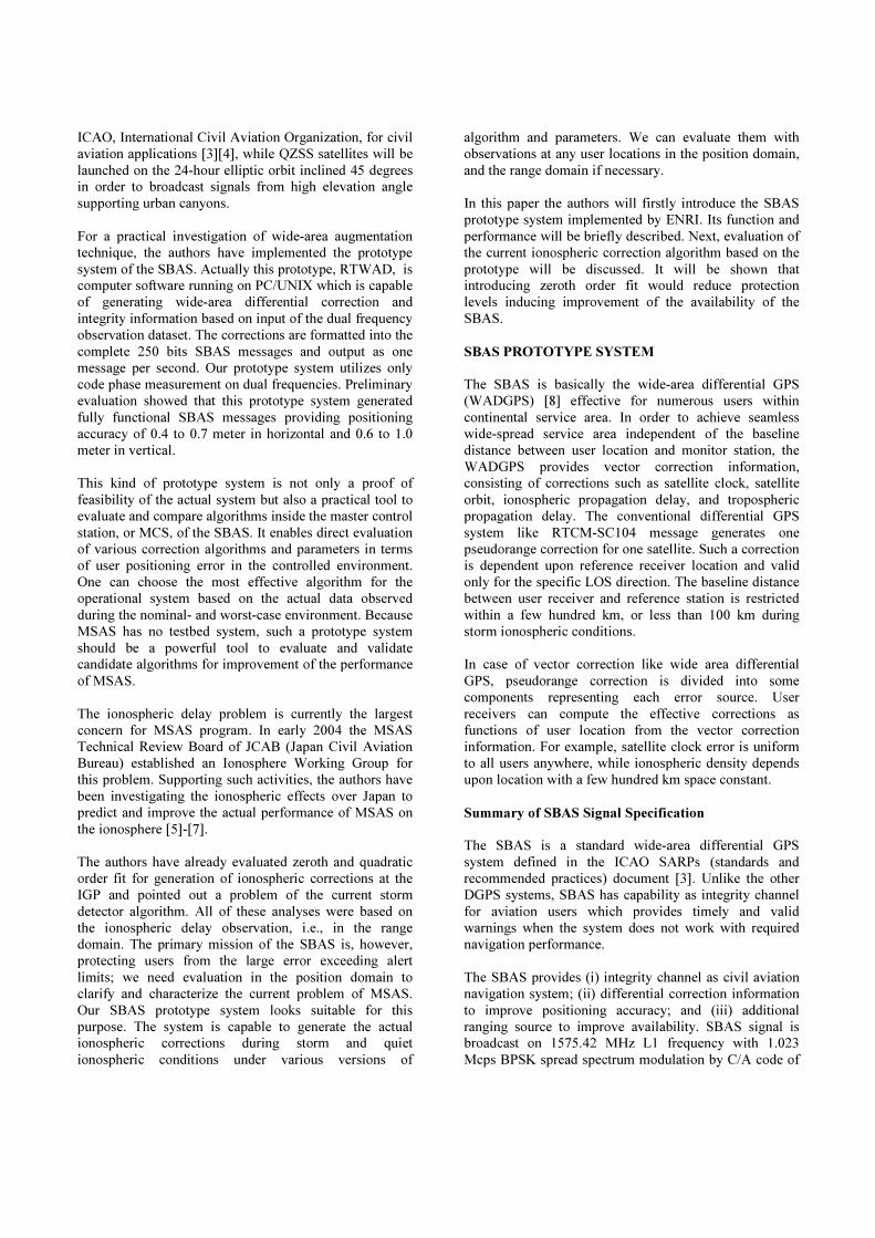
120 135 150

30

45

Longitude, E

Latitude, N

15

30

MLAT

Sata

Sapporo

Hitachi-Ota

Tokyo

Naha

Fukuoka

Kobe

Kochi

Takayama

Oga

Chichijima

Figure 1. Observation stations for the prototype

system. (Red) Monitor stations similar to the MSAS;

(Green) User stations for evaluation.

Table 2. Description of observation stations.

GEONET

ID

Lat

[deg]

Lon

[deg]

Hgt

[m] Location

Monitor Stations

950128 43.0 141.3 205 Sapporo

950214 36.8 140.8 76 Hitachi-Ota

93011 35.9 139.5 63 Tokyo

950356 34.7 135.2 85 Kobe

940087 33.7 130.5 49 Fukuoka

940100 26.1 127.8 128 Naha

User Stations

940030 40.0 139.8 69 Oga

940058 36.1 137.3 813 Takayama

940083 33.5 133.6 71 Kochi

950491 31.1 130.7 368 Sata

92003 27.1 142.2 209 Chichijima

Performance of Prototype System

At first we evaluated the prototype system in terms of

user positioning accuracy. The system has run with

datasets for some periods including both stormy and quiet

ionospheric conditions, and generated SBAS message

streams. Essentially it was able to use any GEONET sites

as monitor stations, we used 6 GEONET sites distributed

similar to the domestic monitor stations of MSAS;

Sapporo, Hitachi-Ota, Tokyo, Kobe, Fukuoka, and Naha,

indicated as Red circles in Figure 1.Their locations are not

exactly identical to the MSAS stations, but similar enough

to know baseline performance comparable with MSAS.

User positioning accuracy was evaluated at 5 GEONET

sites, Green circles in Figure 1. Site 92003 (Chichijima) is

located outside the network of monitor stations, so works

as the sensitive user location in the service area, while

others are on or near to the mainland of Japan. Table 2

summarizes description of monitor stations and user

stations.

Table 3 illustrates the baseline performance of our

prototype system. For quiet ionospheric conditions, the

horizontal accuracy was 0.3 to 0.6 meter and the vertical

error varied 0.4 to 0.8 meter except Site 92003, both in

RMS manner. The ionospheric activities disturbed and

degraded the positioning performance to 2 meters and 3

meters for horizontal and vertical, respectively. Note that

two ionosheric storm events listed in Table 2 are

extremely severe observed only a few times for the last

decade.

In all cases, SBAS receiver simulators computed

horizontal and vertical protection levels as the integrity

requirements. Both horizontal and vertical protection

Table 3. Baseline performance of the prototype system; (Upper) RMS error; (Middle) Max error; (Lower) RMS protection

level; Units are in meters.

940030 940058 940083 950491 92003 Period

Iono-

sphere Hor Ver Hor Ver Hor Ver Hor Ver Hor Ver

Max

δv

2005

11/14-16 Quiet

0.354

1.695

20.02

0.418

2.517

32.11

0.304

1.487

19.41

0.413

2.123

32.18

0.353

1.902

21.62

0.508

4.452

35.46

0.453

3.302

28.37

0.647

6.158

43.97

1.132

6.266

55.34

1.102

5.958

65.38

2.597

2004

11/8-10 Storm

1.546

7.479

101.3

1.900

11.44

152.7

1.157

7.221

91.61

1.560

9.265

146.0

1.057

6.375

89.76

1.559

12.80

154.0

1.639

21.90

100.6

2.195

23.09

167.7

3.302

26.84

109.5

3.427

38.86

188.6

2.019

2004

7/22-24 Active

0.432

2.318

22.56

0.566

4.455

33.69

0.381

2.867

22.08

0.531

5.451

32.58

0.403

2.468

23.13

0.592

4.240

36.99

0.586

2.143

26.59

0.764

5.509

41.24

0.800

4.487

35.58

1.317

9.225

56.11

1.344

2004

6/22-24 Quiet

0.397

2.047

21.73

0.602

4.717

34.32

0.425

2.634

27.00

0.603

3.466

37.69

0.385

1.757

21.39

0.649

3.782

37.82

0.491

2.415

23.14

0.776

4.574

39.36

0.708

4.507

31.32

1.088

6.595

53.77

1.388

2003

10/29-31 Storm

0.982

5.645

127.7

1.057

6.542

181.6

0.659

5.194

191.0

0.840

6.652

231.3

1.407

14.90

152.5

1.863

12.38

249.5

2.164

29.42

144.0

2.901

36.31

229.7

3.121

15.93

129.4

3.356

21.67

216.9

3.135

MSAS Test Signal

2005

11/14-16 Quiet

0.381

1.659

25.82

0.631

2.405

40.48

0.502

4.873

32.83

0.728

3.700

46.29

0.637

8.517

37.67

0.881

9.396

50.08

0.640

3.012

44.34

0.730

2.680

56.24

0.982

6.267

85.79

1.014

6.614

123.0

1.520

Figure 2. Example of user positioning error at Site

940058 on 22-24 July 2004; (Green) Augmented by the

prototype system; (Red) Standalone GPS.

levels have never been exceeded by the associate position

errors regardless of ionospheric activities. This means the

system provided the complete integrity function

protecting users from the large position errors exceeding

protection levels. The maximum errors in Table 2 indicate

that the large errors sometimes occurred, but they were all

within the associate protection levels.

Positioning error was reduced with SBAS messages

produced by the prototype system as shown in Figure 2 in

comparison with standalone mode GPS. The large biases

over 5 meters were eliminated and the error distribution

became compact. The horizontal and vertical error were

improved from 1.929 and 3.305 meters to 0.381 and 0.531

meter, respectively, all in RMS manner.

Figure 3 shows horizontal and vertical user positioning

error at Site 950491 during quiet ionospheric condition on

11/14/05 to 11/16/05. Positioning errors are plotted with

Black, sticking to the horizontal axis. Red curves are the

protection levels therefore they are protecting users with

large margin. They look very conservative but it is

difficult to reduce protection levels due to the stringent 7

10−

integrity requirements.

Verification with MSAS Test Signal

Even MSAS is under operational test, it is sometimes

broadcasting test signal. We have received the test signal

by NovAtel MiLLennium receiver equipped with SBAS

channels at ENRI, Tokyo and decoded it. Test signal was

broadcast continuously for three days from 11/14/05 to

11/16/05.

The SBAS user receiver simulator was again used for this

evaluation. It processed MSAS messages and computed

user position errors in the same way as the previous

section. The performance is summarized in the bottom of

Table 3. The horizontal and vertical RMS accuracies were

0.4 to 0.7 meter and 0.6 to 0.9 meter, respectively, for this

period. Note that this result is based on test signal

obtained only for three days with Message Type 0.

Protection levels of MSAS at Site 950491 are also plotted

as Green curve in Figure 3. Comparing with output of our

prototype system, the protection levels of MSAS were

relatively large. This may represent safety margin as the

first actual operational system. Anyway MSAS also

completely protect users from possible incidental large

errors.

Upcoming Plan; Realtime Operation

Up to now our prototype system has been successfully

implemented and tested. Currently it is operating in

offline mode with past dataset observed and held by

GEONET. As the overall performance, 0.3 to 0.6 meter of

the horizontal accuracy and 0.4 to 0.8 meter of the vertical

accuracy, respectively, both in RMS, were achieved for

quiet ionospheric conditions. Even for the historical

severe ionospheric storm conditions, the accuracies were

degraded to 2 and 3 meters for horizontal and vertical,

respectively. The integrity function worked and always

kept actual user errors within the associate protection

levels.

The next step we are planning is realtime operation. The

software for the prototype is basically driven by Kalman

filter and operating with causality. Therefore only a little

modification will be necessary for realtime operation.

ENRI has already installed 6 realtime monitor stations for

this purpose and additional one is planned to be installed

shortly.

EVALUATION OF IONOSPHERIC CORRECTION

ALGORITHMS

One of possible applications of the prototype SBAS is a

practical evaluation of the algorithms in the MCS. The

authors are responsible to ionospheric problems of MSAS

operating in the low magnetic latitude region, so have

evaluated ionospheric correction algorithms already

proposed in [6] using our prototype system.

Review of the Current Baseline Algorithm

The current baseline algorithm to generate ionospheric

corrections for the SBAS is so-called ‘Planar Fit’ based

on a model of planar ionosphere. Here is a review of the

baseline algorithm [9]-[11].

Figure 3. User positioning error and protection levels

at Site 950491 during quiet ionosphere; (Black) Actual

user error; (Red) Protection levels of the prototype

system; (Green) Protection levels of MSAS.

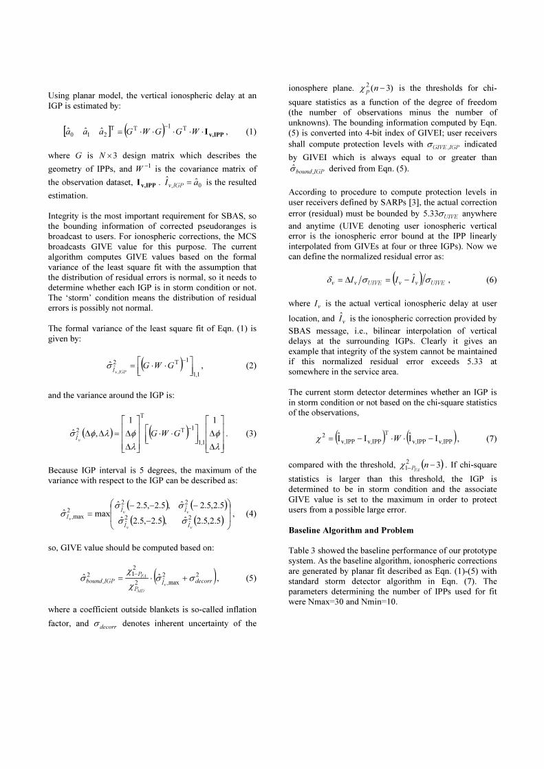
Using planar model, the vertical ionospheric delay at an

IGP is estimated by:

[ ] ( ) v,IPPI⋅⋅⋅⋅⋅=

−

WGGWGaaaT

1TT

210ˆˆˆ , (1)

where G is 3×N design matrix which describes the

geometry of IPPs, and 1−W is the covariance matrix of

the observation dataset, v,IPPI . 0,ˆˆ aI

IGPv= is the resulted

estimation.

Integrity is the most important requirement for SBAS, so

the bounding information of corrected pseudoranges is

broadcast to users. For ionospheric corrections, the MCS

broadcasts GIVE value for this purpose. The current

algorithm computes GIVE values based on the formal

variance of the least square fit with the assumption that

the distribution of residual errors is normal, so it needs to

determine whether each IGP is in storm condition or not.

The ‘storm’ condition means the distribution of residual

errors is possibly not normal.

The formal variance of the least square fit of Eqn. (1) is

given by:

( )1,1

1T2ˆ,

ˆ

⋅⋅=

−

GWGIGPvI

σ , (2)

and the variance around the IGP is:

( ) ( )

∆

∆

⋅⋅

∆

∆=∆∆−

λ

φ

λ

φλφσ

11

,ˆ1,1

1T

T

2ˆ GWGvI

. (3)

Because IGP interval is 5 degrees, the maximum of the

variance with respect to the IGP can be described as:

( ) ( )

( ) ( )

−

−−−=

5.2,5.2ˆ,5.2,5.2ˆ

5.2,5.2ˆ,5.2,5.2ˆmaxˆ

2ˆ

2ˆ

2ˆ

2ˆ2

max,

vv

vv

v

II

II

Iσσ

σσ

σ , (4)

so, GIVE value should be computed based on:

( )22

max,ˆ2

212

,ˆˆ

decorrI

P

P

IGPboundv

MD

FAσσ

χ

χσ +⋅=

−

, (5)

where a coefficient outside blankets is so-called inflation

factor, and decorr

σ denotes inherent uncertainty of the

ionosphere plane. )3(2 −np

χ is the thresholds for chi-

square statistics as a function of the degree of freedom

(the number of observations minus the number of

unknowns). The bounding information computed by Eqn.

(5) is converted into 4-bit index of GIVEI; user receivers

shall compute protection levels with IGPGIVE ,

σ indicated

by GIVEI which is always equal to or greater than

IGPbound,σ derived from Eqn. (5).

According to procedure to compute protection levels in

user receivers defined by SARPs [3], the actual correction

error (residual) must be bounded by UIVE

σ33.5 anywhere

and anytime (UIVE denoting user ionospheric vertical

error is the ionospheric error bound at the IPP linearly

interpolated from GIVEs at four or three IGPs). Now we

can define the normalized residual error as:

( )UIVEvvUIVEvv

III σσδ ˆ−=∆= , (6)

where vI is the actual vertical ionospheric delay at user

location, and vI is the ionospheric correction provided by

SBAS message, i.e., bilinear interpolation of vertical

delays at the surrounding IGPs. Clearly it gives an

example that integrity of the system cannot be maintained

if this normalized residual error exceeds 5.33 at

somewhere in the service area.

The current storm detector determines whether an IGP is

in storm condition or not based on the chi-square statistics

of the observations,

( ) ( )IPPv,IPPv,

T

IPPv,IPPv,2

IIII −⋅⋅−= Wχ , (7)

compared with the threshold, ( )32

1−

−

nFAP

χ . If chi-square

statistics is larger than this threshold, the IGP is

determined to be in storm condition and the associate

GIVE value is set to the maximum in order to protect

users from a possible large error.

Baseline Algorithm and Problem

Table 3 showed the baseline performance of our prototype

system. As the baseline algorithm, ionospheric corrections

are generated by planar fit described as Eqn. (1)-(5) with

standard storm detector algorithm in Eqn. (7). The

parameters determining the number of IPPs used for fit

were Nmax=30 and Nmin=10.

According to Table 3, protection levels increase much

during ionospheric storm condition. RMS VPL was over

100 meters everywhere even while the largest vertical

positioning error was up to 36 meters at the southern

locations. If protection levels are reduced down to the

levels of the largest position errors, the system could

deliver APV-I operation capability anytime anywhere and

also APV-II capability to most of Japan. The SBAS could

not provide APV operations unless protection levels are

reduced enough less than alert limits, even if the

positioning accuracy were greatly improved. It is not

necessary, so far, to improve accuracy; reducing

protection levels is the most important and urgent

problem for the current SBAS architecture.

Figure 4 illustrates VPL and ionospheric component of

VPL during storm ionosphere. VPL grows large daytime,

but decreases to the levels of quiet ionospheric condition

(also see Figure 3) in nighttime. This implies that VPL is

affected largely by the ionosphere. In fact, seeing

ionospheric component of VPL (Blue curve), it is clear

that most of VPL was come from ionosphere and effects

of other components (UDRE and troposphere) are little. It

is necessary to reduce ionospheric component of VPL, i.e.

GIVE (grid ionospheric vertical error), to achieve smaller

VPL for better system availability.

Ionosphere is the dominant term in computation of

Protection Levels, while Table 3 indicates the actual

largest error is much smaller than protection levels. Let us

see relationship between vertical ionospheric correction

residuals and UIVE (user ionospheric vertical error)

shown in Figure 5. 5.33 UIVE overbounds the actual

residuals with a large margin regardless of the magnitude

of the actual residuals. Note that these examples are

observed during the historical severe magnetic storm

conditions. There is no doubt that overbounding the actual

residuals is the fundamental purpose of UIVE, but such

margin looks too conservative and in fact sacrifice the

system availability.

UIVE is provided as shown in Figure 6 without the storm

detector algorithm. Comparing Figures 5 and 6, the large

UIVE is resulted in by trip of storm detector. It is

important that the actual ionospheric residual exceeded

5.33 UIVE only once (at 03/10/31 14:40:00, lower right

in Figure 6) even there is no storm detector. The storm

detector certainly protects users from possible large

ionospheric residual exceeding 5.33 UIVE, however there

were only a few effective true alerts even during storm

ionospheric conditions and the others are all false alerts.

Introduction of Zeroth Order Fit

The ionospheric storm detector described in Eqn. (7)

caused a lot of false alert conditions lowering system

availability. To avoid such a problem there are two

possible ways:

(i) Develop an alternative safety mechanism instead

of the storm detector;

(ii) Develop a method to compute GIVE values

instead of setting to the maximum when storm

detector trips.

Figure 5. Observed vertical ionospheric residual error

at Site 950491 during storm ionosphere; (Black)

Actual residual error; (Red) 5.33 UIVE.

Figure 4. Vertical Protection Levels at Site 950491

during storm ionospheric condition; (Black) Actual

user error; (Red) VPL; (Blue) Ionospheric component

of VPL.

The authors have already proposed both algorithms. An

overbounding algorithm based on geometry monitor

concept was described in [7] as method (i); and the zeroth

order fit [6] is also available as method (ii). Here we have

tried the zeroth order fit, the latter method, as follows.

According to the standard storm detector algorithm [9],

GIVE will be set to the maximum (GIVE=45m;

GIVEI=14) if chi-square statistics exceeded the threshold

for the associate IGP. Chi-square statistics is computed by

Eqn. (7) therefore large chi-square means planar model is

not applicable to the associate IGP because the

distribution of fit residuals from the plane is no longer the

normal.

It is still possible to apply any ionosphere models other

than planar even if chi-square test determined planar

model is not applicable. There are many possible

algorithms; one way is decreasing the order of fit. It is

quite reasonable to decrease the order of estimation, or to

reduce the number of unknown parameters to be

estimated, is quite reasonable when the observation is

noisy or the exact model is unknown. We have little

knowledge on the physical structure of stormy ionosphere

so far, then increasing the order is not recommended for

such a condition.

We employ the zeroth order fit when the storm detector

trips or the number of IPP is insufficient. Even for the

zeroth order, the above procedure for generating

Ionospheric corrections in Eqn. (1) to (5) needs no

modifications. Note that the design matrix G becomes

1×N . In order to increase availability of ionospheric

corrections, parameters determining the number of IPPs

for fit are set to 5,10minmax

== NN .

At first, the zeroth order fit algorithm without the storm

detector was implemented in our prototype system and

evaluated during storm ionospheric conditions. No

adaptive algorithms are implemented at this step; the

zeroth order fit always applied. Table 4 summarizes

resulted performance. Comparing with Table 3, RMS

Figure 7. Vertical ionospheric residual error and

UIVE produced by the zeroth order fit; (Black) Actual

residual error; (Red) 5.33 UIVE. Note that the large

residual at 03/10/31 14:40:00, indicated by the black

arrow, is also bounded within 4.823 UIVE.

Figure 6. UIVE without the storm detector algorithm.

Compare with Figure 5.

Table 4. Performance by the zeroth order fit; (Upper) RMS error; (Middle) Max error; (Lower) RMS Protection Level;

Units are in meters.

940030 940058 940083 950491 92003 Period

Iono-

sphere Hor Ver Hor Ver Hor Ver Hor Ver Hor Ver

Max

δv

2004

11/8-10 Storm

1.520

8.653

30.93

1.657

9.725

49.36

0.957

7.435

25.60

1.455

11.24

43.28

0.961

6.713

28.53

1.495

12.77

48.00

1.443

9.788

35.71

2.062

11.34

58.89

2.929

18.76

44.31

3.086

20.81

75.37

2.940

2003

10/29-31 Storm

0.916

4.047

35.04

1.164

6.826

55.02

0.528

5.242

33.09

0.701

6.269

52.63

1.107

11.56

43.63

1.428

11.56

68.06

1.773

14.74

45.22

2.239

19.56

70.62

3.420

15.82

46.35

3.531

17.53

80.89

4.823

position accuracies are slightly improved, and, more

importantly, protection levels are reduced down to one

third relative to the current algorithm.

Figure 7 illustrates relationship between the actual

vertical ionospheric delay and UIVE produced by the

zeroth order fit. The largest normalized residuals of

ionospheric corrections, v

δ , were 2.940 and 4.823, both

less than 5.33, for two periods of November 2004 and

October 2003, respectively. The large residual at 03/10/31

14:40:00, indicated by the black arrow, is also bounded

within 4.823 UIVE. This means that the ionospheric

correction residuals are protected enough by UIVE even

during the most severe storm condition and no additional

mechanism like the storm detector is necessary for the

zeroth order fit.

Adaptive Algorithm

The zeroth order fit has capability of keeping the actual

ionospheric correction residuals within 5.33 UIVE so it

does not need additional algorithm like the storm detector.

The zeroth order fit means actually simple weighted

average so this is robust estimation.

As the authors previously reported, the zeroth order fit

can be performed in case that the number of IPPs is

insufficient in order to improve availability of the

ionospheric corrections as well as when the storm detector

trips [6]. Here we introduce an adaptive algorithm as

follows;

1. Apply the standard planar fit with the storm

detector;

2. If storm detector does not trip, employ resulted

correction and GIVE;

3. Otherwise, or the number of IPPs is insufficient

for the standard planar fit, perform the zeroth

order fit.

Clearly this algorithm would reduce the maximum GIVEI

events (GIVEI=14) because the zeroth order fit possibly

produces lower GIVEI when the storm detector trips.

Figure 8 compares the distribution of GIVEI produced

during a storm event in November 2004. By using the

adaptive algorithm GIVEI were reduced to 13 which

means 559.4,

=IGPGIVE

σ m for most of IGPs, while the

baseline algorithm produced the maximum GIVEI=14

relating to 68.13,

=IGPGIVE

σ m for 50% of IGPs.

Figure 9 shows an example of vertical protection levels

produced by the adaptive algorithm during storm

ionospheric conditions. Comparing with Figure 4, VPL

were reduced down to one third relative to the current

Figure 8. Distribution of GIVEI during storm iono-

spheric condition in November 2004; (Red) Baseline

algorithm; (Blue) Adaptive algorithm reduced the

maximum GIVEI=14.

Table 5 Performance of the adaptive algorithm; (Upper) RMS error; (Middle) Max error; (Lower) RMS Protection Level;

Units are in meters.

940030 940058 940083 950491 92003 Period

Iono-

sphere Hor Ver Hor Ver Hor Ver Hor Ver Hor Ver

Max

δv

2005

11/14-16 Quiet

0.360

2.130

19.50

0.421

2.517

31.49

0.305

1.723

18.75

0.414

2.344

31.64

0.339

1.377

19.10

0.510

4.631

33.79

0.468

4.160

21.22

0.643

3.748

37.18

1.219

5.763

51.10

1.184

6.175

59.34

2.597

2004

11/8-10 Storm

1.507

8.343

27.31

1.662

9.697

41.83

0.953

7.457

22.93

1.449

11.28

37.36

0.973

6.641

24.69

1.482

13.08

41.05

1.430

9.505

29.73

2.035

11.30

48.65

2.987

18.69

38.26

3.184

32.01

65.21

2.940

2004

7/22-24 Active

0.431

2.318

33.27

0.561

4.684

40.77

0.381

2.867

32.05

0.533

5.451

39.22

0.396

1.998

35.51

0.589

3.766

42.17

0.581

2.152

37.30

0.772

4.359

44.16

0.823

3.243

52.28

1.352

11.85

62.42

1.665

2004

6/22-24 Quiet

0.396

2.197

32.90

0.602

4.775

39.72

0.424

2.634

35.61

0.600

3.550

43.30

0.384

1.757

36.01

0.645

3.930

42.04

0.490

2.415

37.74

0.771

4.755

44.34

0.708

2.771

51.92

1.078

6.790

60.40

1.388

2003

10/29-31 Storm

0.916

4.047

32.73

1.194

6.918

48.88

0.532

5.219

31.32

0.689

4.938

47.87

1.138

11.81

40.14

1.456

10.00

61.95

1.788

14.74

41.13

2.256

19.56

64.01

3.453

15.56

44.01

3.513

18.06

73.00

4.823

baseline. This means the adaptive algorithm will

contribute to improve the availability of the SBAS

In fact, the adaptive algorithm achieved the performance

shown in Table 5. Like the performance of the zeroth

order fit, RMS position accuracies are slightly improved

and protection levels are reduced down to one third

relative to the baseline algorithm. The protection levels

are further improved from the zeroth order fit, with

sacrifice of slight degradation of positioning accuracies.

The largest normalized residual of ionospheric corrections

were within 5.33 for every period including the historical

severe storm conditions.

Table 6 compares availability of the SBAS for APV-I

operation which requires HAL=40m and VAL=50m

between two algorithms. The proposed adaptive algorithm

improves availability to 60-80% over mainland of Japan.

However, it is still necessary to further reduce protection

levels for operations in the southern part of Japan.

CONCLUDING REMARKS

The authors firstly reported the performance of the

prototype system of SBAS successfully implemented and

tested by ENRI. It generated the complete SBAS message

stream and evaluated with the SBAS receiver simulator.

For quiet ionospheric conditions, the horizontal accuracy

was 0.3 to 0.6 meter and the vertical error varied 0.4 to

0.8 meter, both in RMS manner. The historical severe

ionospheric activities might disturb and degraded the

positioning performance to 2 meters and 3 meters for

horizontal and vertical, respectively.

In all cases, both horizontal and vertical protection levels

have never been exceeded by the associate position errors

regardless of ionospheric activities. This means the

system provided the complete integrity function

protecting users from the large position errors inducing

integrity break.

As an application of this prototype system, the authors

evaluated the current and improved ionospheric correction

algorithms in a practical manner. It is operational problem

that protection levels tend to grow large based on

productions of the current algorithm. It was shown that

the proposed algorithm of adaptive switching between the

planar and zeroth order fit reduced protection levels down

to one third relative to the current baseline algorithm. The

availability of APV-I operation was improved to 60-80%

over mainland of Japan for storm ionospheric conditions.

The prototype system is useful tool for this kind of

evaluation of the algorithms inside MCS of the SBAS.

Further analysis will be performed using the prototype

towards APV-II operations. There is also a plan to operate

the prototype system in online mode with realtime

monitor stations being installed.

REFERENCES

[1] J. Imamura, MSAS Program and Overview, Proc. 4th

CGSIC IISC Asia Pacific Rim Meeting, 2003 Joint Int’l

Conference on GPS/GNSS, Tokyo, Nov. 2003.

[2] H. Maeda, QZSS Overview and Interoperability, Proc.

18th Int’l Tech. Meeting of the Satellite Division of the

Institute of Navigation (ION GNSS), Plenary Session,

Long Beach, CA, Sept. 2005.

[3] International Standards and Recommended Practices,

Table 6 Availability for APV-I operation; (Upper) Baseline algorithm; (Lower) Adaptive algorithm.

Period Ionosphere 940030 940058 940083 950491 92003

2004

11/8-10 Storm

37.1 %

77.6 %

36.9 %

86.8 %

39.1 %

81.6 %

38.3 %

68.7 %

25.7 %

33.8 %

2003

10/29-31 Storm

28.4 %

59.0 %

25.9 %

62.1 %

15.8 %

34.9 %

19.9 %

33.9 %

14.0 %

18.7 %

Figure 9. Vertical Protection Levels at Site 950491

during storm ionospheric condition by the adaptive

algorithm; (Black) Actual user error; (Red) VPL;

(Blue) Ionospheric component of VPL. Compare with

Figure 4 with care about the vertical axes.

Aeronautical Telecommunications, Annex 10 to the Con-

vention on International Civil Aviation, vol. I, ICAO, Nov.

2002.

[4] Minimum Operational Performance Standards for

Global Positioning System/Wide Area Augmentation Sys-

tem Airborne Equipment, DO-229C, RTCA, Nov. 2001.

[5] T. Sakai, K. Matsunaga, K. Hoshinoo, and T. Walter,

Evaluating Ionospheric Effects on SBAS in the Low

Magnetic Latitude Region, Proc. 17th Int’l Tech. Meeting

of the Satellite Division of the Institute of Navigation

(ION GNSS), pp. 1318-1328, Long Beach, CA, Sept. 2004.

[6] T. Sakai, K. Matsunaga, K. Hoshinoo, T. Walter,

Improving Availability of Ionospheric Corrections in the

Low Magnetic Latitude Region, Proc. ION National

Technical Meeting, pp. 569-579, San Diego, CA, Jan.

2005.

[7] T. Sakai, K. Matsunaga, K. Hoshinoo, and T. Walter,

Modified Ionospheric Correction Algorithm for the SBAS

Based on Geometry Monitor Concept, Proc. 18th Int’l

Tech. Meeting of the Satellite Division of the Institute of

Navigation (ION GNSS), pp. 735-747, Long Beach, CA,

Sept. 2005.

[8] Changdon Kee, Wide Area Differential GPS, Global

Positioning System: Theory and Applications, II, Chap. 3,

pp. 81-115, AIAA, 1996.

[9] T. Walter, A. Hansen, J. Blanch, P. Enge, T.

Mannucci, X. Pi, L. Sparks, B. IIjima, B. El-Arini, R.

Lejeune, M. Hagen, E. Altshuler, R. Fries, and A. Chu,

Robust Detection of Ionospheric Irregularities, Proc. 13th

Int’l Tech. Meeting of the Satellite Division of the Institute

of Navigation (ION GPS), pp. 209-218, Salt Lake City,

UT, Sept. 2000.

[10] A. Komjathy, L. Sparks, A. Mannucci, and X. Pi, An

Assessment of the Current WAAS Ionospheric Correction

Algorithm in the South American Region, Navigation: J.

Institute of Navigation, vol. 50, no. 3, pp. 193-204, Fall

2003.

[11] L. Sparks, A. Komjathy, and A. Mannucci, Sudden

Ionospheric Delay Decorrelation and Its Impact on the

Wide Area Augmentation System (WAAS), Radio

Science, vol. 39, RS1S13, 2004.