Protein Structure Prediction, Second Edition€¦ · computational methods to understand the nature of protein–protein interactions, one of which is protein–protein docking. This

11

Protein–Protein Docking: Overview and PerformanceAnalysis

Kevin Wiehe, Matthew W. Peterson, Brian Pierce, Julian Mintseris,and Zhiping Weng

Summary

Protein–protein docking is the computational prediction of protein complex structure giventhe individually solved component protein structures. It is an important means for under-standing the physicochemical forces that underlie macromolecular interactions and a valuabletool for modeling protein complex structures. Here, we report an overview of protein–proteindocking with specific emphasis on our Fast Fourier Transform-based rigid-body docking programZDOCK, which is consistently rated as one of the most accurate docking programs in the CriticalAssessment of Predicted Interactions (CAPRI), a series of community-wide blind tests. We alsoinvestigate ZDOCK’s performance on a non-redundant protein complex benchmark. Finally, weperform regression analysis to better understand the strengths and weaknesses of ZDOCK andto suggest areas of future development for protein-docking algorithms in general.

Key Words: Protein–protein docking; ZDOCK; RDOCK; Fast Fourier Transform; benchmark;CAPRI; shape complementarity; electrostatics; desolvation energy; regression analysis.

1. IntroductionProtein–protein interactions play a central role in biochemistry. This can

be seen in cell-signaling cascades, enzyme catalysis, the immune responseby means of antibody–antigen interactions, and the large-scale motions oforganisms. These interactions are also implicated in many diseases.

From: Methods in Molecular Biology, Vol. 413: Protein Structure Prediction, Second EditionEdited by: M. Zaki and C. Bystroff © Humana Press Inc., Totowa, NJ

283

284 Wiehe et al.

While experimental techniques such as yeast two-hybrid system and massspectrometry are able to determine the existence of protein–protein interactions,the structure of the macromolecular complex of two interacting proteins canprovide additional information about their interaction, such as the specificresidues involved in the interaction and the degree of conformational changeundergone by the proteins upon binding.

X-ray crystallography and nuclear magnetic resonance have provided uswith the structures of many complexes, but numerous structures still remainunsolved because of time and experimental limitations. This leads to a need forcomputational methods to understand the nature of protein–protein interactions,one of which is protein–protein docking.

This chapter is divided into three sections. The first section provides anoverview of protein–protein docking and describes some of the availablealgorithms for docking. The second describes the ZDOCK suite of programsin detail, and the third describes an analysis of the performance of ZDOCK.

1.1. Protein–Protein Docking: An Overview

Protein–protein docking is defined as the prediction of the structure of twoproteins in a complex, given only the structure of the interacting proteins. The“docking problem” can be broken down into two types of docking: bounddocking, in which a complex is separated and reassembled, and unbounddocking, where the structure of the complex is found from the individuallysolved structures of the interacting proteins. Obviously, bound docking haslittle applicable value, but it is often used for testing and verification purposes.

Unbound docking is much more difficult than bound docking because theproteins involved can change conformation upon binding. A study of confor-mational changes in protein complexes (1) showed that while the general modelfor protein–protein recognition is an induced fit model where the proteins mustchange conformation in order to bind, the amount of conformational changewas small enough such that binding could be modeled as a “lock-and-key”mechanism as a first approximation. This allows for successful docking resultseven when there are noticeable changes in the conformation of the inter-acting proteins. This “rigid-body” approximation has been invaluable in theadvancement of the protein–protein docking field. However, modeling inducedfit by flexible docking remains a central challenge, and a large portion ofcurrent docking research is focused in this area.

There are two main challenges in the development of methods for protein–protein docking. The first is the construction of a scoring function that allowsfor the discrimination between correct or near-correct predictions and incorrectpredictions. The second is the development of an algorithm that quickly searchesand scores all possible orientations of the proteins to be docked. The most

Protein–Protein Docking 285

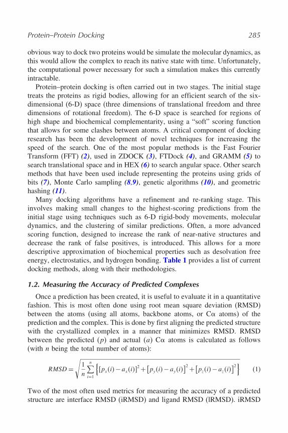
obvious way to dock two proteins would be simulate the molecular dynamics, asthis would allow the complex to reach its native state with time. Unfortunately,the computational power necessary for such a simulation makes this currentlyintractable.

Protein–protein docking is often carried out in two stages. The initial stagetreats the proteins as rigid bodies, allowing for an efficient search of the six-dimensional (6-D) space (three dimensions of translational freedom and threedimensions of rotational freedom). The 6-D space is searched for regions ofhigh shape and biochemical complementarity, using a “soft” scoring functionthat allows for some clashes between atoms. A critical component of dockingresearch has been the development of novel techniques for increasing thespeed of the search. One of the most popular methods is the Fast FourierTransform (FFT) (2), used in ZDOCK (3), FTDock (4), and GRAMM (5) tosearch translational space and in HEX (6) to search angular space. Other searchmethods that have been used include representing the proteins using grids ofbits (7), Monte Carlo sampling (8,9), genetic algorithms (10), and geometrichashing (11).

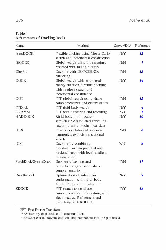
Many docking algorithms have a refinement and re-ranking stage. Thisinvolves making small changes to the highest-scoring predictions from theinitial stage using techniques such as 6-D rigid-body movements, moleculardynamics, and the clustering of similar predictions. Often, a more advancedscoring function, designed to increase the rank of near-native structures anddecrease the rank of false positives, is introduced. This allows for a moredescriptive approximation of biochemical properties such as desolvation freeenergy, electrostatics, and hydrogen bonding. Table 1 provides a list of currentdocking methods, along with their methodologies.

1.2. Measuring the Accuracy of Predicted Complexes

Once a prediction has been created, it is useful to evaluate it in a quantitativefashion. This is most often done using root mean square deviation (RMSD)between the atoms (using all atoms, backbone atoms, or C� atoms) of theprediction and the complex. This is done by first aligning the predicted structurewith the crystallized complex in a manner that minimizes RMSD. RMSDbetween the predicted (p) and actual (a) C� atoms is calculated as follows(with n being the total number of atoms):

RMSD =√

1n

n∑i=1

{�px�i�−ax�i��

2 + [py�i�−ay�i�]2 + [pz�i�−az�i�

]2}

(1)

Two of the most often used metrics for measuring the accuracy of a predictedstructure are interface RMSD (iRMSD) and ligand RMSD (lRMSD). iRMSD

286 Wiehe et al.

Table 1A Summary of Docking Tools

Name Method Server/DLa Reference

AutoDOCK Flexible docking using Monte Carlosearch and incremental construction

N/Y 12

BiGGER Global search using bit mapping,rescored with multiple filters

N/N 7

ClusPro Docking with DOT/ZDOCK,clustering

Y/N 13

DOCK Global search with grid-basedenergy function, flexible dockingwith random search andincremental construction

N/Y 14

DOT FFT global search using shapecomplementarity and electrostatics

Y/N 15

FTDock FFT rigid-body search N/Y 4GRAMM FFT with clustering and rescoring Y/Y 5HADDOCK Rigid-body minimization,

semi-flexible simulated annealing,rescoring using biochemical data

N/Y 16

HEX Fourier correlation of sphericalharmonics, explicit translationalsearch

Y/N 6

ICM Docking by combiningpseudo-Brownian potential andtorsional steps with local gradientminimization

N/Nb 8

PatchDock/SymmDock Geometric hashing andpose-clustering to score shapecomplementarity

Y/N 17

RosettaDock Optimization of side-chainconformation with rigid- bodyMonte Carlo minimization

N/Y 9

ZDOCK FFT search using shapecomplementarity, desolvation, andelectrostatics. Refinement andre-ranking with RDOCK

Y/Y 18

FFT, Fast Fourier Transform.a Availability of download to academic users.b Browser can be downloaded; docking component must be purchased.


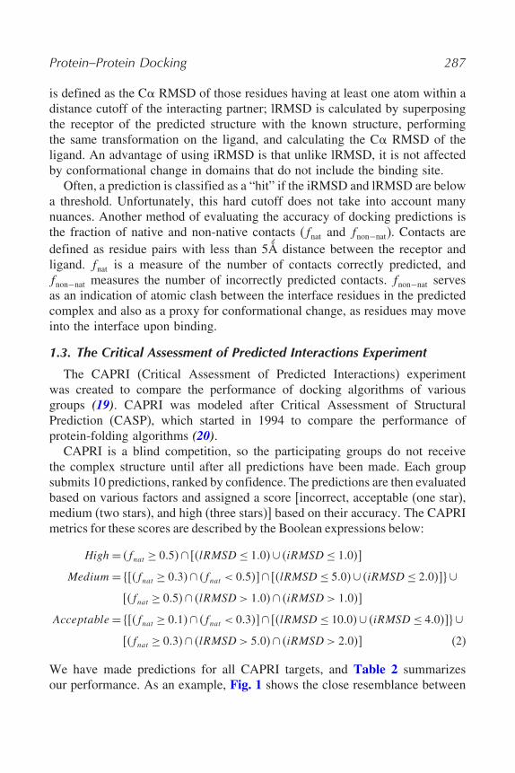
is defined as the C� RMSD of those residues having at least one atom within adistance cutoff of the interacting partner; lRMSD is calculated by superposingthe receptor of the predicted structure with the known structure, performingthe same transformation on the ligand, and calculating the C� RMSD of theligand. An advantage of using iRMSD is that unlike lRMSD, it is not affectedby conformational change in domains that do not include the binding site.

Often, a prediction is classified as a “hit” if the iRMSD and lRMSD are belowa threshold. Unfortunately, this hard cutoff does not take into account manynuances. Another method of evaluating the accuracy of docking predictions isthe fraction of native and non-native contacts (fnat and fnon−nat). Contacts aredefined as residue pairs with less than 5Å distance between the receptor andligand. fnat is a measure of the number of contacts correctly predicted, andfnon−nat measures the number of incorrectly predicted contacts. fnon−nat servesas an indication of atomic clash between the interface residues in the predictedcomplex and also as a proxy for conformational change, as residues may moveinto the interface upon binding.

1.3. The Critical Assessment of Predicted Interactions Experiment

The CAPRI (Critical Assessment of Predicted Interactions) experimentwas created to compare the performance of docking algorithms of variousgroups (19). CAPRI was modeled after Critical Assessment of StructuralPrediction (CASP), which started in 1994 to compare the performance ofprotein-folding algorithms (20).

CAPRI is a blind competition, so the participating groups do not receivethe complex structure until after all predictions have been made. Each groupsubmits 10 predictions, ranked by confidence. The predictions are then evaluatedbased on various factors and assigned a score [incorrect, acceptable (one star),medium (two stars), and high (three stars)] based on their accuracy. The CAPRImetrics for these scores are described by the Boolean expressions below:

High = �fnat ≥ 0�5�∩ ��lRMSD ≤ 1�0�∪ �iRMSD ≤ 1�0��

Medium = ��fnat ≥ 0�3�∩ �fnat < 0�5��∩ ��lRMSD ≤ 5�0�∪ �iRMSD ≤ 2�0��∪��fnat ≥ 0�5�∩ �lRMSD > 1�0�∩ �iRMSD > 1�0��

Acceptable = ��fnat ≥ 0�1�∩ �fnat < 0�3��∩ ��lRMSD ≤ 10�0�∪ �iRMSD ≤ 4�0��∪��fnat ≥ 0�3�∩ �lRMSD > 5�0�∩ �iRMSD > 2�0�� (2)

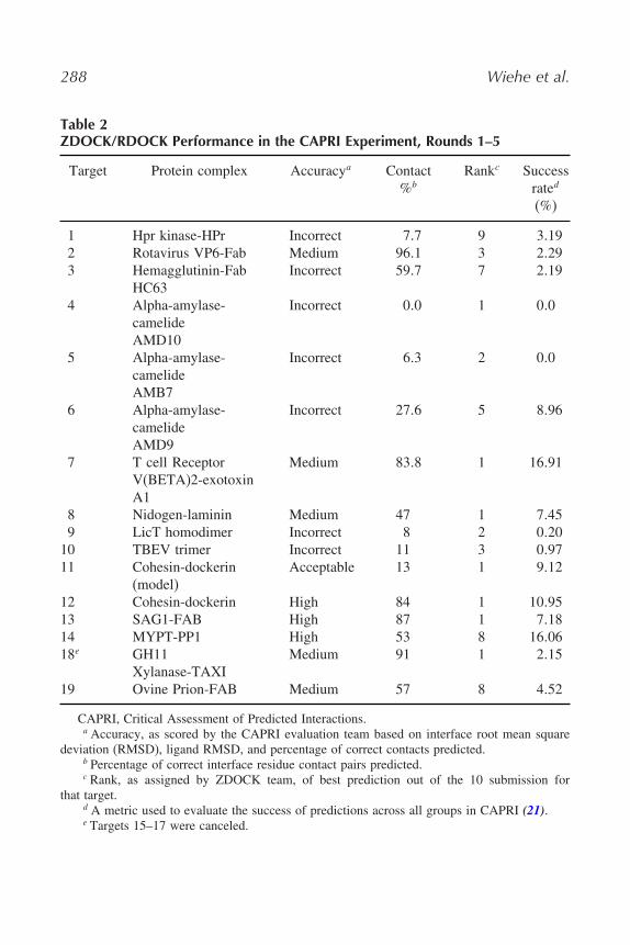
We have made predictions for all CAPRI targets, and Table 2 summarizesour performance. As an example, Fig. 1 shows the close resemblance between

288 Wiehe et al.

Table 2ZDOCK/RDOCK Performance in the CAPRI Experiment, Rounds 1–5

Target Protein complex Accuracya Contact%b

Rankc Successrated

(%)

1 Hpr kinase-HPr Incorrect 7�7 9 3�192 Rotavirus VP6-Fab Medium 96�1 3 2�293 Hemagglutinin-Fab

HC63Incorrect 59�7 7 2�19

4 Alpha-amylase-camelideAMD10

Incorrect 0�0 1 0�0

5 Alpha-amylase-camelideAMB7


6 Alpha-amylase-camelideAMD9


7 T cell ReceptorV(BETA)2-exotoxinA1

Medium 83�8 1 16�91

8 Nidogen-laminin Medium 47 1 7�459 LicT homodimer Incorrect 8 2 0�20

10 TBEV trimer Incorrect 11 3 0�9711 Cohesin-dockerin

(model)Acceptable 13 1 9�12

12 Cohesin-dockerin High 84 1 10�9513 SAG1-FAB High 87 1 7�1814 MYPT-PP1 High 53 8 16�0618e GH11

Xylanase-TAXIMedium 91 1 2�15

19 Ovine Prion-FAB Medium 57 8 4�52

CAPRI, Critical Assessment of Predicted Interactions.a Accuracy, as scored by the CAPRI evaluation team based on interface root mean square

deviation (RMSD), ligand RMSD, and percentage of correct contacts predicted.b Percentage of correct interface residue contact pairs predicted.c Rank, as assigned by ZDOCK team, of best prediction out of the 10 submission for

that target.d A metric used to evaluate the success of predictions across all groups in CAPRI (21).e Targets 15–17 were canceled.


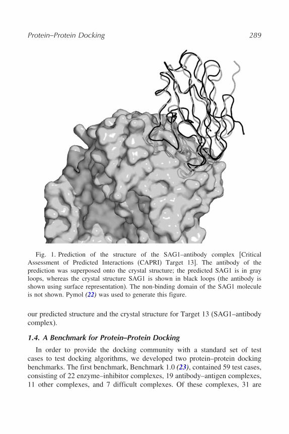
Fig. 1. Prediction of the structure of the SAG1–antibody complex [CriticalAssessment of Predicted Interactions (CAPRI) Target 13]. The antibody of theprediction was superposed onto the crystal structure; the predicted SAG1 is in grayloops, whereas the crystal structure SAG1 is shown in black loops (the antibody isshown using surface representation). The non-binding domain of the SAG1 moleculeis not shown. Pymol (22) was used to generate this figure.

our predicted structure and the crystal structure for Target 13 (SAG1–antibodycomplex).

1.4. A Benchmark for Protein–Protein Docking

In order to provide the docking community with a standard set of testcases to test docking algorithms, we developed two protein–protein dockingbenchmarks. The first benchmark, Benchmark 1.0 (23), contained 59 test cases,consisting of 22 enzyme–inhibitor complexes, 19 antibody–antigen complexes,11 other complexes, and 7 difficult complexes. Of these complexes, 31 are

290 Wiehe et al.

unbound–unbound, and 28 are bound–unbound. A number of groups have usedthis benchmark to test the performance of their docking algorithms (9,24–26).

A newer version of the docking benchmark, Benchmark 2.0 (27), has beencreated. It includes 84 test cases and was designed to focus on unbound–unbound test cases. Structural classification of proteins (SCOPs) (28) was usedto avoid redundancy in the benchmark. This benchmark is classified by dockingdifficulty, based on the amount of conformational change undergone by theinteracting proteins. Complexes classified as rigid and medium fall into therealm of rigid-body docking, whereas complexes classified as difficult wouldrequire algorithms that explicitly search backbone conformations.

2. The ZDOCK/RDOCK/M-ZDOCK Approach2.1. ZDOCK: An FFT-Based Initial Stage Docking Algorithm

ZDOCK is an initial-stage docking algorithm that uses an FFT to find thethree-dimensional (3-D) structure of a protein complex. The ZDOCK algorithmoptimizes three parameters: shape complementarity, electrostatics, and desol-vation free energy.

ZDOCK takes Protein Data Bank (PDB) (29) files as input. The larger of thetwo interacting proteins is considered the receptor (R), whereas the smaller ofthe two is considered the ligand (L). These PDB files are first parsed throughthe supplied program mark_sur, which measures the amount of accessiblesurface area (ASA) of each atom using a water probe of radius 1.4 Å. If anatom has an ASA of more than 1 Å2, it is marked as a surface atom. mark_suralso marks the atom type for each atom in the structure, based on the 18 atomtypes based on atomic contact energy (ACE) (30). For any given rotationalorientation, the L and R are both discretized onto a 3-D grid of size N ×N ×Nwith a spacing of 1.2 Å. N must be large enough such that the grid can coverthe sum of the maximal spans of R and L, plus 1.2 Å, and it is often set at 128.

2.1.1. The Fast Fourier Transform

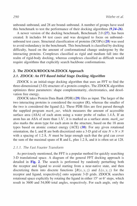
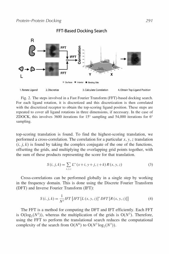
As previously mentioned, the FFT is a popular method for quickly searching3-D translational space. A diagram of the general FFT docking approach isdetailed in Fig. 2. The search is performed by randomly perturbing boththe receptor and ligand to avoid starting from a near-native state, and thendiscretizing them into discrete functions �R�x y z� and L�x y z� for thereceptor and ligand, respectively] onto separate 3-D grids. ZDOCK searchesrotational space explicitly by rotating the ligand in either 15� or 6� steps, whichresult in 3600 and 54,000 total angles, respectively. For each angle, only the


Fig. 2. The steps involved in a Fast Fourier Transform (FFT)-based docking search.For each ligand rotation, it is discretized and this discretization is then correlatedwith the discretized receptor to obtain the top-scoring ligand position. These steps arerepeated to cover all ligand rotations in three dimensions, if necessary. In the case ofZDOCK, this involves 3600 iterations for 15� sampling and 54,000 iterations for 6�

sampling.

top-scoring translation is found. To find the highest-scoring translation, weperformed a cross-correlation. The correlation for a particular x y z translation�i j k� is found by taking the complex conjugate of the one of the functions,offsetting the grids, and multiplying the overlapping grid points together, withthe sum of these products representing the score for that translation.

S �i j k� = ∑xyz

L∗ �x+ i y + j z+k�R�x y z� (3)

Cross-correlations can be performed globally in a single step by workingin the frequency domain. This is done using the Discrete Fourier Transform(DFT) and Inverse Fourier Transform (IFT):

S �i j k� = 1N 3

IFT{IFT �L �x y z��∗ DFT �R�x y z��

}(4)

The FFT is a method for computing the DFT and IFT efficiently. Each FFTis O�log2�N

3��, whereas the multiplication of the grids is O�N 3�. Therefore,using the FFT to perform the translational search reduces the computationalcomplexity of the search from O�N 6� to O�N 3 log2�N

3��.

292 Wiehe et al.

ZDOCK uses a combination of three physical and biochemical properties todescribe ligand and receptor: shape complementarity, desolvation free energy,and electrostatics.

2.1.2. Shape Complementarity

The physical basis for shape complementarity comes from the van der Waals(vdW) potential. Atoms are subject to an attractive force at long distances, anda repulsive force at short distances, caused by the overlap of electronic orbitals.Most often, this is approximated by the Lennard–Jones 6–12 potential, shownbelow:

VL−J = A

r12− B

r6(5)

The r6term represents the attractive energy, whereas the r12 term represents therepulsive energy. The minimum of the vdW potential is found at the sum ofthe vdW radii, which can be thought of as the effective sizes of the interactingatoms.

Early versions of ZDOCK used a shape complementarity function knownas grid-based shape complementarity (GSC) (3). Here, two discrete functions,RGSC (GSC function for the receptor) and LGSC (GSC function for the ligand),are used to describe the geometric characteristics of the two proteins as follows:

RGSC =

⎧⎪⎪⎨⎪⎪⎩

1 solvent-accessible surface9i solvent-excluding surface9i core0 open space

LGSC =

⎧⎪⎪⎨⎪⎪⎩

0 solvent-accessible surface1 solvent-excluding surface9i core0 open space

(7)

The solvent-excluding surface layer is defined by the grid points marked assurface atoms by mark_sur, whereas the core is defined as the atoms not onthe surface. The solvent-accessible surface layer is an additional layer of gridpoints surrounding the surface of the protein.

The current version of ZDOCK uses a complementarity function known aspairwise shape complementarity (PSC) (31). PSC is composed of a favorableterm and a penalty term. The favorable term calculates the number of atom pairsbetween R and L within a distance cutoff D, whereas the penalty componentof PSC is proportional to the number of overlapping grid points between


R and L, much like GSC. Whereas the GSC function results in grid spaces withpurely real or imaginary values, the PSC function is complex. LPSC and RPSC

are shown below.

� [Lpsc

]={

1 if nearest grid point to ligand atom0 otherwise

� [Rpsc

]=⎧⎨⎩

Number of receptor atoms within D = +vdW radiusof nearest atom open space

0 otherwise

�LPSC� = �RPSC� =⎧⎨⎩

3 solvent-excluding surface9 core0 open space

(8)

The use of PSC rather than GSC for scoring shape complementarity was shownto greatly increase the number of near-native predictions for Benchmark 1.0during initial stage docking (31).

2.1.3. Desolvation Free Energy and Electrostatics

ACE (30) is used by ZDOCK to estimate desolvation free energy. ACE isdefined as the change in free energy resulting from the breaking of two atom–water contacts and the formation of an atom–atom contact and a water–watercontact. This is also referred to as the hydrophobic effect, which is known toplay a critical role in protein–protein binding. ZDOCK introduces two discretefunctions, LDE and RDE, to describe the desolvation energy of the ligand andreceptor:

� �LDE� = � �RDE� ={

PSC+ACE scores of all nearby atoms open space0 otherwise

�LDE� = �RDE� ={

1 if nearest grid point to atom0 otherwise

(9)

The electrostatics energy term for ZDOCK can be expressed as a correlationbetween the electric potential generated by the receptor with the charges of theligand atoms. ZDOCK adopts the Coulombic formula used by Gabb et al. (4)but incorporates partial charges using the CHARMM19 parameters from theCHARMM molecular mechanics program (32).

2.1.4. ZDOCK Scoring Function

There are two ZDOCK versions that use PSC to describe shape complemen-tarity: ZDOCK 2.1 simply uses PSC as the scoring function, whereas ZDOCK

294 Wiehe et al.

2.3 uses a linear combination of the shape complementarity-electrostatics scoreand the desolvation score. ZDOCK 2.3 incorporates PSC and electrostatics intosingle complex functions (RPSC+ELEC and LPSC+ELEC� to improve computationtime. These functions are described below:

� [LPSC+ELEC

]= � [RPSC+ELEC

]=⎧⎨⎩

3�5 solvent-excluding surface3�52 core0 open space

[RPSC+ELEC

]={

�∗ electric potential of all R atoms open space0 otherwise

[LPSC+ELEC

]={−1∗ atom charge grid point closes to ligand atom

0 otherwise(10)

2.2. RDOCK: Refining ZDOCK Predictions

The refinement stage of protein docking with ZDOCK is carried out usingan algorithm known as RDOCK (33). Because of the soft scoring functionin ZDOCK, many of the top-scoring predictions are false positives (not near-native). RDOCK refines these output structures through energy minimization.This is carried out in three steps, using CHARMM (32).

1. Removal of clashes by minimization of vdW and internal energies.2. Minimization of total (Coulombic electrostatics, vdW, internal) energy, constraining

non-hydrogen atoms, and keeping ionic side chains in their neutral states.3. Minimization of total energy with no restrictions.

Once energy minimization has been performed, the minimized structures arere-ranked. Any complexes that still exhibit clashes (those that have vdW energyof 10 kcal/mol or greater) after minimization are discarded. Electrostatics anddesolvation energy for the complexes are calculated using CHARMM and ACE,respectively. The RDOCK scoring function, �Gbinding, is a linear combinationof desolvation score (�GACE� and electrostatic energy (�Eelec�.

�Gbinding = �GACE +0�9∗�EELEC (11)

2.3. M-ZDOCK: Symmetric Multimer Docking with ZDOCK

The ZDOCK algorithm has been modified to predict the structure of Cn

multimer complexes, in which two or more identical proteins interact, resultingin a ring-shaped complex. M-ZDOCK (34) reconstructs the multimer based onthe optimal position of two adjacent monomers in a single plane. This leads toa reduction in computational time due to the reduced search space, as well asan increase in performance when compared with docking Cn multimers withZDOCK.


2.4. ZDOCK Performance on Benchmark 2.0

ZDOCK was tested against version 2.0 of the docking benchmark usingZDOCK 2.3 and ZDOCK 2.1, with 6� and 15� angular sampling.

2.4.1. Prediction Evaluation

To evaluate the structure predictions produced by ZDOCK, we used theRMSD of the interface C� atoms. Interface C� atoms were identified byselecting residues that had any atom within 10 Å of the other molecule in thebound complex. A hit was defined as a prediction with an iRMSD ≤ 2�5 Å.

Two measures are defined to evaluate the average performance of a dockingalgorithm over the entire benchmark. Success rate is defined as the percentageof test cases that have a hit in the top N predictions. Average hit count is thenumber of hits for all test cases in the top N predictions, divided by the numberof test cases.

2.4.2. Running ZDOCK

Several considerations were taken before and while running ZDOCK. Toremove bias from the starting positions (the Benchmark 2.0 unbound test casesare by default aligned to the bound proteins, to facilitate the evaluation ofpredicted structures), we used a different random seed to rotate the ligand foreach case. In addition, the antibodies (apart from the camelid 1KXQ) had mostof their non-complementarity-determining region (non-CDR) loops blocked toavoid false-positive predictions. The CDRs of the antibodies were identifiedusing their sequences (loops L1, L2, L3, H1, H2, and H3) and by examinationof the structures (loops L4 and H4 and the N-termini).

2.4.3. Success Rate and Hit Count

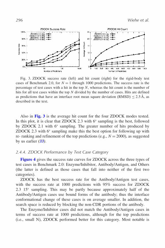
Figure 3 shows the success rate for ZDOCK when run against all rigid-bodycases from Benchmark 2.0. It can be seen that ZDOCK 2.3 performs betteroverall than ZDOCK 2.1 in terms of success rate. This is because the scoringfunction used in ZDOCK 2.3 is better at discriminating hits against incorrectpredictions across the benchmark. Also, for both ZDOCK 2.1 and ZDOCK2.3, the 15� sampling has a higher success rate than the 6� sampling. Thisindicates that for more predictions (i.e., finer sampling), there are more falsepositives introduced that reduce the rank of the first hit in some of the testcases. However, the 6� sampling is superior with regard to the number of hits,indicated by the hit count plot.

296 Wiehe et al.

Fig. 3. ZDOCK success rate (left) and hit count (right) for the rigid-body testcases of Benchmark 2.0, for N = 1 through 1000 predictions. The success rate is thepercentage of test cases with a hit in the top N , whereas the hit count is the number ofhits for all test cases within the top N divided by the number of cases. Hits are definedas predictions that have an interface root mean square deviation (RMSD) ≤ 2�5 Å, asdescribed in the text.

Also in Fig. 3 is the average hit count for the four ZDOCK modes tested.In this plot, it is clear that ZDOCK 2.3 with 6� sampling is the best, followedby ZDOCK 2.1 with 6� sampling. The greater number of hits produced byZDOCK 2.3 with 6� sampling make this the best option for following up withre- ranking and refinement of the top predictions (e.g., N = 2000), as suggestedby us earlier (33).

2.4.4. ZDOCK Performance by Test Case Category

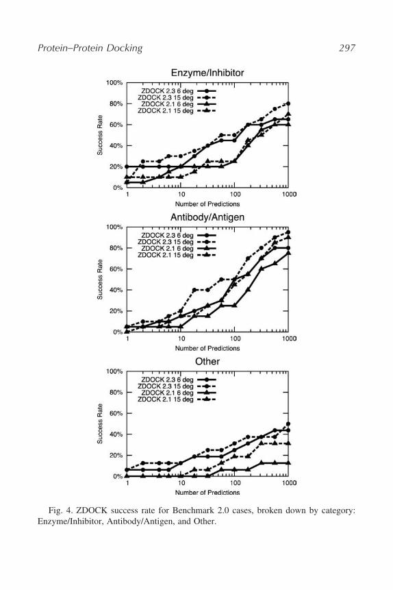
Figure 4 gives the success rate curves for ZDOCK across the three types oftest cases in Benchmark 2.0: Enzyme/Inhibitor, Antibody/Antigen, and Others(the latter is defined as those cases that fall into neither of the first twocategories).

ZDOCK has the best success rate for the Antibody/Antigen test cases,with the success rate at 1000 predictions with 95% success for ZDOCK2.3 15� sampling. This may be partly because approximately half of theAntibody/Antigen cases use bound forms of the antibody; thus the interfaceconformational change of these cases is on average smaller. In addition, thesearch space is reduced by blocking the non-CDR portions of the antibody.

The Enzyme/Inhibitor cases did not match the Antibody/Antigen cases interms of success rate at 1000 predictions, although for the top predictions(i.e., small N), ZDOCK performed better for this category. Most notable is


Fig. 4. ZDOCK success rate for Benchmark 2.0 cases, broken down by category:Enzyme/Inhibitor, Antibody/Antigen, and Other.

298 Wiehe et al.

the 20% success for ZDOCK 2.3 15� sampling for the top prediction (four of20 cases). This may be due to the PSC scoring function, which when combinedwith desolvation and electrostatics (as in ZDOCK 2.3) is well suited to identifythe pocket-shaped binding sites on the enzymes.

ZDOCK did not perform quite as well on the Others test cases; this was alsoseen when ZDOCK was run against Benchmark 1.0 Others test cases. Of thefour ZDOCK options tested, both sampling levels of ZDOCK 2.3 performedbetter than ZDOCK 2.1. In fact, at N = 1000, ZDOCK 2.3 still performedbetter than ZDOCK 2.1, whereas for Enzyme/Inhibitor and Antibody/Antigencases, the ZDOCK 2.1 15� sampling performed better than ZDOCK 2.3 6�

sampling. This trend may indicate that shape complementarity (which is theonly scoring metric used for ZDOCK 2.1) is less important (versus electro-statics and desolvation) for the Others cases than for the Enzyme/Inhibitor andAntibody/Antigen cases.

2.5. Docking Overview: Summary

Protein–protein docking has evolved to the point where it is possible topredict the structures of many protein complexes based on their unboundproteins. This is demonstrated above using a protein-docking benchmark andthe rigid-body-docking algorithm ZDOCK. However, based on the success rateplots of Fig. 3, it is evident that not all cases are successfully predicted withinthe top few thousand docking predictions, and for a few cases, no hits arefound. What leads to this variation in docking success across a set of cases? Thefinal section of this chapter takes an in-depth look at how various propertiesof proteins impact the ability of docking to successfully predict the complexstructure.

3. The Relationships Between ZDOCK Performance and ProteinComplex Characteristics

The performance of ZDOCK is dependent on both the accuracy of theenergy function and the comprehensiveness of the search algorithm. Both ofthese are in turn dependent on the many physicochemical characteristics of theprotein–protein complex that ZDOCK is attempting to predict. For example,in any particular complex, the exact shape of the protein–protein interfacewill undoubtedly have an effect on how high shape complementarity is scoredin the energy function. Protein–protein complexes with planar interfaces mayprove to be the most challenging for ZDOCK. Thus, it is important to examinehow ZDOCK performs with respect to differing interface shapes in order togauge the effectiveness of the shape complementarity term. Knowing how


ZDOCK performs with respect to a vast array of different protein–proteincomplex characteristics provides an understanding of what types of complexesZDOCK can be expected to excel in predicting. It also can help lead to morefocused improvements in the development of protein docking by identifyingthe strengths and weaknesses of the algorithm. In addition, it may be possibleto extend the conclusions drawn from such an examination to other FFT-baseddocking algorithms.

3.1. Near-Native Prediction Definitions

In order to objectively and systematically evaluate the performance of theZDOCK algorithm, it is necessary to compare the near-native docking orien-tations produced by ZDOCK to the space of orientations available given aparticular complex within the rigid-body FFT framework. While the fieldsof protein structure prediction and docking commonly make use of “decoys”to evaluate algorithm performance, here we adopt an alternative approach.We estimate the space of potential near-native conformations using a newlydesigned program called HitFinder. This space is reasonably limited under theassumption of rigid-body docking, and therefore focus was placed on the 64rigid-body cases from the protein-docking benchmark (27).

Using the core framework of the ZDOCK algorithm, HitFinder maps thecomplex components onto a 1�2 Å grid and uses a 6� Euler angle set (18)to perform FFT search for orientations that would represent near-native hits.HitFinder iterates over the same set of angles and translations as ZDOCK butuses a simple RMSD filter instead of a docking scoring function. For everypotential ligand-docking orientation where the ligand overlaps with the nativeligand orientation, the docking orientation is retained for further processing ifthe ligand C RMSD is less than or equal to 10 Å. Following this initial search,potential docking hits are further defined using a more nuanced protocol basedon the CAPRI prediction accuracy criteria. As in CAPRI, these hit definitionsrely on the combination of RMSD and native contact fraction criteria. Here twokinds of hits are classified: high quality and medium quality. They are definedby the following Boolean relationships:

High-quality hits = [iRMSD ≤ (

iRMSDsuperposed unbound complex +1 Å)]

∩ �fnat > 0�5�∩ �fnon-nat < 0�5� (12)

Medium-quality hits = [iRMSD ≤ (

iRMSDsuperposed unbound complex +1 Å)]

∩ �fnat > 0�3�∩ �fnon-nat < 0�7� (13)

300 Wiehe et al.

Because HitFinder does not include the shape complementarity functionsthat are normally a part of the ZDOCK algorithm, there is no control overpotential ligand/receptor clash for those orientations where they come too closeto each other. Therefore, this study uses the more strictly defined space ofhigh-quality hits (or three-star hits; Eq. 2) as a guide and eliminates all hits withclash significantly greater than the average three-star hit. Clashes are definedas the number of interface contacts within 3 Å. All docking orientations witha clash total greater than the mean number of clashes for the three-star hitsplus 2 standard deviations are eliminated. Finally, if an orientation meets allthe required hit criteria, it is labeled a “potential hit” and all such structures arerecorded for a complex.

3.2. Measuring ZDOCK Success

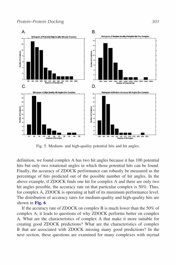
To examine the success of ZDOCK, a metric for protein–protein dockingaccuracy is needed. Measuring ZDOCK accuracy per complex could be accom-plished by merely counting the number of medium- or high-quality hits thealgorithm achieves out of a certain number of predictions. However, because thenumber of potential hits is inherent to each particular protein–protein complex(see Fig. 5A and B), this measure would not reflect precisely how well ZDOCKperforms. As an example, if complex A has 100 potential hits and complex Bhas 1000 potential hits, ZDOCK’s accuracy is not equivalent if it finds onehit for both complexes. Complex B is easier to predict because it possessessome characteristics that allow for a greater number of hits possible. Furtherdiscussion as to what characteristics these may be will follow in Section 3.It may make sense to simply take the percentage of hits predicted out ofthe number of potential hits as a metric for docking accuracy. In this metric,ZDOCK makes successful predictions at a 1% rate for complex A and only a0.1% rate for complex B and thus clearly performs better on complex A. Yetthere is a flaw to this measure as well. As explained previously, the ZDOCKalgorithm only keeps the highest-scoring translation for every rotation anglesearched. This means that if multiple hits exist in the same rotational angle,ZDOCK will at best only select one of them. In the example of complex Aversus complex B, complex A has 100 potential hits, but hypothetically couldhave 99 in one rotational angle. In that case, the highest number of hits anoptimal ZDOCK search could find would only be 2. Thus, accuracy as definedas a percentage of potential hits would reach the upper limit at 2%. It isnecessary then to introduce another definition, that of the “hit angle.” A hitangle is defined as any rotational angle in a ZDOCK search that has at leastone translation that results in a potential hit (see Fig. 5C and D). Using this


Fig. 5. Medium- and high-quality potential hits and hit angles.

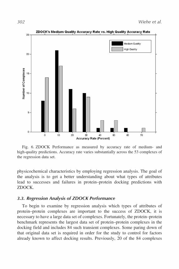
definition, we found complex A has two hit angles because it has 100 potentialhits but only two rotational angles in which those potential hits can be found.Finally, the accuracy of ZDOCK performance can robustly be measured as thepercentage of hits predicted out of the possible number of hit angles. In theabove example, if ZDOCK finds one hit for complex A and there are only twohit angles possible, the accuracy rate on that particular complex is 50%. Thus,for complex A, ZDOCK is operating at half of its maximum performance level.The distribution of accuracy rates for medium-quality and high-quality hits areshown in Fig. 6.

If the accuracy rate of ZDOCK on complex B is much lower than the 50% ofcomplex A, it leads to questions of why ZDOCK performs better on complexA. What are the characteristics of complex A that make it more suitable forcreating good ZDOCK predictions? What are the characteristics of complexB that are associated with ZDOCK missing many good predictions? In thenext section, these questions are examined for many complexes with myriad

302 Wiehe et al.

Fig. 6. ZDOCK Performance as measured by accuracy rate of medium- andhigh-quality predictions. Accuracy rate varies substantially across the 53 complexes ofthe regression data set.

physicochemical characteristics by employing regression analysis. The goal ofthe analysis is to get a better understanding about what types of attributeslead to successes and failures in protein–protein docking predictions withZDOCK.

3.3. Regression Analysis of ZDOCK Performance

To begin to examine by regression analysis which types of attributes ofprotein–protein complexes are important to the success of ZDOCK, it isnecessary to have a large data set of complexes. Fortunately, the protein–proteinbenchmark represents the largest data set of protein–protein complexes in thedocking field and includes 84 such transient complexes. Some paring down ofthat original data set is required in order for the study to control for factorsalready known to affect docking results. Previously, 20 of the 84 complexes


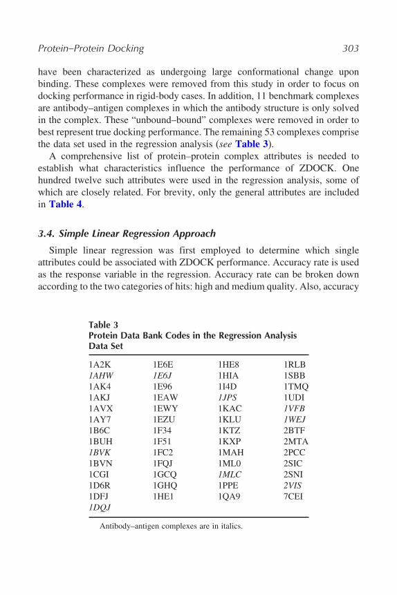
have been characterized as undergoing large conformational change uponbinding. These complexes were removed from this study in order to focus ondocking performance in rigid-body cases. In addition, 11 benchmark complexesare antibody–antigen complexes in which the antibody structure is only solvedin the complex. These “unbound–bound” complexes were removed in order tobest represent true docking performance. The remaining 53 complexes comprisethe data set used in the regression analysis (see Table 3).

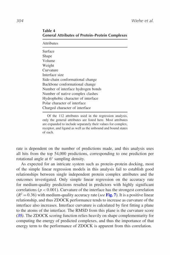
A comprehensive list of protein–protein complex attributes is needed toestablish what characteristics influence the performance of ZDOCK. Onehundred twelve such attributes were used in the regression analysis, some ofwhich are closely related. For brevity, only the general attributes are includedin Table 4.

3.4. Simple Linear Regression Approach

Simple linear regression was first employed to determine which singleattributes could be associated with ZDOCK performance. Accuracy rate is usedas the response variable in the regression. Accuracy rate can be broken downaccording to the two categories of hits: high and medium quality. Also, accuracy

Table 3Protein Data Bank Codes in the Regression AnalysisData Set

1A2K 1E6E 1HE8 1RLB1AHW 1E6J 1HIA 1SBB1AK4 1E96 1I4D 1TMQ1AKJ 1EAW 1JPS 1UDI1AVX 1EWY 1KAC 1VFB1AY7 1EZU 1KLU 1WEJ1B6C 1F34 1KTZ 2BTF1BUH 1F51 1KXP 2MTA1BVK 1FC2 1MAH 2PCC1BVN 1FQJ 1ML0 2SIC1CGI 1GCQ 1MLC 2SNI1D6R 1GHQ 1PPE 2VIS1DFJ 1HE1 1QA9 7CEI1DQJ

Antibody–antigen complexes are in italics.

304 Wiehe et al.

Table 4General Attributes of Protein–Protein Complexes

Attributes

SurfaceShapeVolumeWeightCurvatureInterface sizeSide-chain conformational changeBackbone conformational changeNumber of interface hydrogen bondsNumber of native complex clashesHydrophobic character of interfacePolar character of interfaceCharged character of interface

Of the 112 attributes used in the regression analysis,only the general attributes are listed here. Most attributesare expanded to include separately their values for complex,receptor, and ligand as well as the unbound and bound statesof each.

rate is dependent on the number of predictions made, and this analysis usesall hits from the top 54,000 predictions, corresponding to one prediction perrotational angle at 6� sampling density.

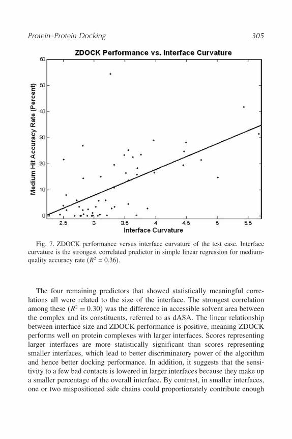
As expected for an intricate system such as protein–protein docking, mostof the simple linear regression models in this analysis fail to establish goodrelationships between single independent protein complex attributes and theoutcomes investigated. Only simple linear regression on the accuracy ratefor medium-quality predictions resulted in predictors with highly significantcorrelations �p < 0�001�. Curvature of the interface has the strongest correlation�R2 = 0�36� with medium-quality accuracy rate (see Fig. 7). It is a positive linearrelationship, and thus ZDOCK performance tends to increase as curvature of theinterface also increases. Interface curvature is calculated by first fitting a planeto the atoms of the interface. The RMSD from this plane is the curvature score(35). The ZDOCK scoring function relies heavily on shape complementarity forcomputing the energy of predicted complexes, and thus the importance of thatenergy term to the performance of ZDOCK is apparent from this correlation.


Fig. 7. ZDOCK performance versus interface curvature of the test case. Interfacecurvature is the strongest correlated predictor in simple linear regression for medium-quality accuracy rate (R2 = 0.36).

The four remaining predictors that showed statistically meaningful corre-lations all were related to the size of the interface. The strongest correlationamong these �R2 = 0�30� was the difference in accessible solvent area betweenthe complex and its constituents, referred to as dASA. The linear relationshipbetween interface size and ZDOCK performance is positive, meaning ZDOCKperforms well on protein complexes with larger interfaces. Scores representinglarger interfaces are more statistically significant than scores representingsmaller interfaces, which lead to better discriminatory power of the algorithmand hence better docking performance. In addition, it suggests that the sensi-tivity to a few bad contacts is lowered in larger interfaces because they make upa smaller percentage of the overall interface. By contrast, in smaller interfaces,one or two mispositioned side chains could proportionately contribute enough

306 Wiehe et al.

high energy to the overall docking score to sufficiently lower the rank of anear-native structure such that it is not included in the final prediction set.

3.5. Multiple Linear Regression Approach

Whereas simple linear regression is an important first look at which singlecharacteristics of protein complexes are relevant to the performance of ZDOCK,a more comprehensive approach should involve the employment of multiplelinear regression analysis. Finding the relationship of combined attributes toZDOCK sampling and accuracy gives a better indication of what to expect interms of successes and failures depending on the type of complex involvedin the prediction. In multiple linear regression, it is important to avoid over-fitting the data caused by using a small ratio of outcome variables to predictorvariables. Therefore in this study, only sets of four attributes were consideredfor the regression with 53 complexes. It was computationally tractable to dothe regression on all permutations of four attributes and thus avoid the pitfallsassociated with a stepwise regression approach.

3.5.1. Medium Quality Predictions

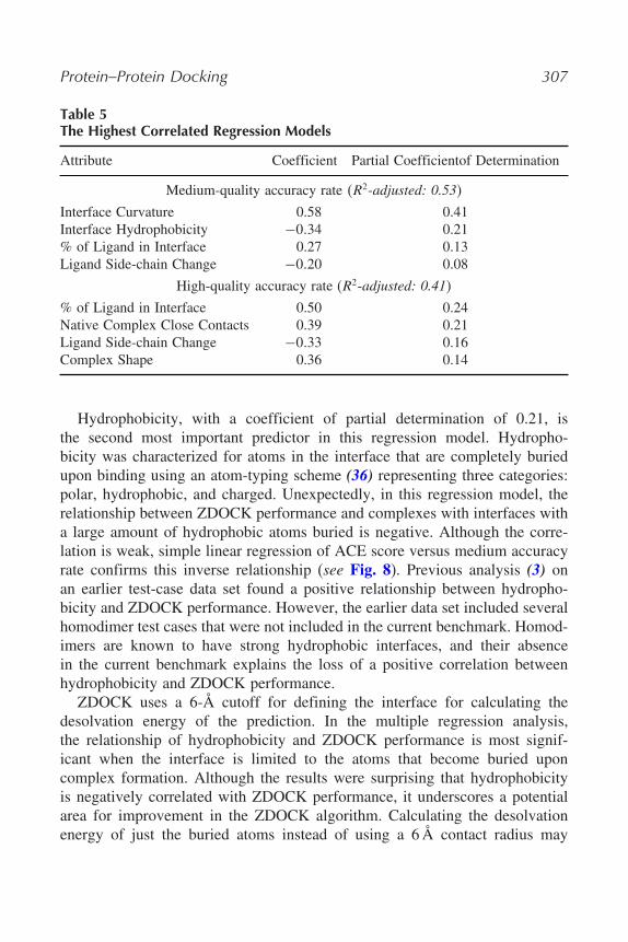
Multiple linear regression analysis was computed for the response variables ofaccuracy rate for medium- and high-quality hits with four predictors. For medium-qualityaccuracyrate, the fourattributeswith thehighestcorrelation(R2 adjusted =0�53) were: curvature of the interface, size of the ligand interface relative to the sizeof the ligand, ligand side-chain conformational change, and the hydrophobicity ofatoms that are completely buried upon binding (see Table 5).

The inclusion of curvature of interface in the top correlated set of attributessuggests the importance of shape complementarity just as it did in the simplelinear regression for medium-quality accuracy rate. It is possible to exactlydetermine how important interface curvature or any other predictor is to theoverall correlation by looking at the coefficients of partial determination forthe regression model. A coefficient of partial determination in this analysismeasures the proportionate reduction in variation in ZDOCK performance whena particular predictor is included in the regression model. With the above fourattributes, the coefficient of partial determination for the inclusion of interfacecurvature in the regression model is 0.41. This explains quantitatively thatinterface curvature accounts for a 41% reduction in the regression error whenit is added to the three-attribute model of interface hydrophobicity, ligand side-chain conformational change, and ligand interface size relative to the size ofthe ligand. Thus, interface curvature is highly important to the multiple linearrelationship between these four predictors and ZDOCK performance.


Table 5The Highest Correlated Regression Models

Attribute Coefficient Partial Coefficientof Determination

Medium-quality accuracy rate �R2-adjusted: 0.53�

Interface Curvature 0.58 0.41Interface Hydrophobicity −0�34 0.21% of Ligand in Interface 0.27 0.13Ligand Side-chain Change −0�20 0.08

High-quality accuracy rate (R2-adjusted: 0.41�

% of Ligand in Interface 0.50 0.24Native Complex Close Contacts 0.39 0.21Ligand Side-chain Change −0�33 0.16Complex Shape 0.36 0.14

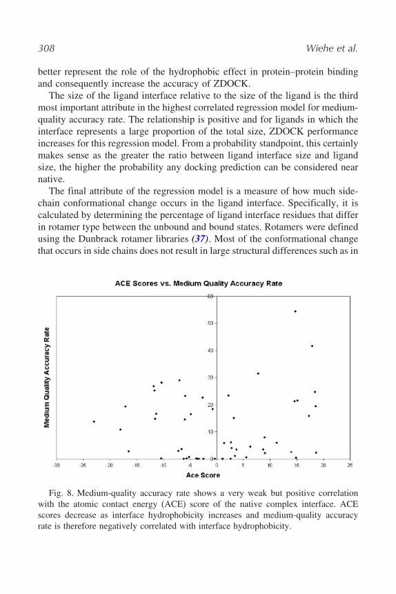
Hydrophobicity, with a coefficient of partial determination of 0.21, isthe second most important predictor in this regression model. Hydropho-bicity was characterized for atoms in the interface that are completely buriedupon binding using an atom-typing scheme (36) representing three categories:polar, hydrophobic, and charged. Unexpectedly, in this regression model, therelationship between ZDOCK performance and complexes with interfaces witha large amount of hydrophobic atoms buried is negative. Although the corre-lation is weak, simple linear regression of ACE score versus medium accuracyrate confirms this inverse relationship (see Fig. 8). Previous analysis (3) onan earlier test-case data set found a positive relationship between hydropho-bicity and ZDOCK performance. However, the earlier data set included severalhomodimer test cases that were not included in the current benchmark. Homod-imers are known to have strong hydrophobic interfaces, and their absencein the current benchmark explains the loss of a positive correlation betweenhydrophobicity and ZDOCK performance.

ZDOCK uses a 6-Å cutoff for defining the interface for calculating thedesolvation energy of the prediction. In the multiple regression analysis,the relationship of hydrophobicity and ZDOCK performance is most signif-icant when the interface is limited to the atoms that become buried uponcomplex formation. Although the results were surprising that hydrophobicityis negatively correlated with ZDOCK performance, it underscores a potentialarea for improvement in the ZDOCK algorithm. Calculating the desolvationenergy of just the buried atoms instead of using a 6 Å contact radius may

308 Wiehe et al.

better represent the role of the hydrophobic effect in protein–protein bindingand consequently increase the accuracy of ZDOCK.

The size of the ligand interface relative to the size of the ligand is the thirdmost important attribute in the highest correlated regression model for medium-quality accuracy rate. The relationship is positive and for ligands in which theinterface represents a large proportion of the total size, ZDOCK performanceincreases for this regression model. From a probability standpoint, this certainlymakes sense as the greater the ratio between ligand interface size and ligandsize, the higher the probability any docking prediction can be considered nearnative.

The final attribute of the regression model is a measure of how much side-chain conformational change occurs in the ligand interface. Specifically, it iscalculated by determining the percentage of ligand interface residues that differin rotamer type between the unbound and bound states. Rotamers were definedusing the Dunbrack rotamer libraries (37). Most of the conformational changethat occurs in side chains does not result in large structural differences such as in

Fig. 8. Medium-quality accuracy rate shows a very weak but positive correlationwith the atomic contact energy (ACE) score of the native complex interface. ACEscores decrease as interface hydrophobicity increases and medium-quality accuracyrate is therefore negatively correlated with interface hydrophobicity.


the complexes with backbone conformational change that were removed in thecreation of the data set. However, even small differences in side-chain positionscan cause large inaccuracies in the calculation of the scoring function especiallywithin the vdW terms. Because ZDOCK does not attempt to move side chainsduring docking, interfaces with more side chains in different positions than intheir unbound state will cause an inaccurate representation of the true boundinterface and thus ZDOCK performance will suffer. Side-chain search is anactively pursued area in protein–protein docking research, and from the resultsof this regression analysis, it is understandable why accurate placement of sidechains is a vital part of making successful docking predictions.

3.5.2. High-Quality Predictions

In comparison to the ability of ZDOCK to produce medium–quality predic-tions, there may exist a different set of characteristics of protein complexes thatassociate with ZDOCK’s ability to generate high-quality predictions.

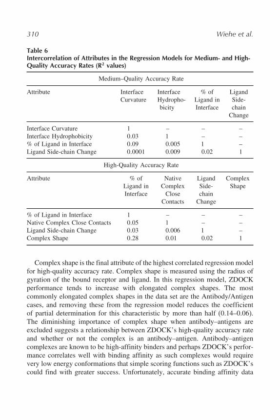
To this end, all regression models with four predictors were run using thehigh-quality accuracy rate as the response variable. The highest correlatedmodel (R2 adjusted = 0�40) included the following four attributes: complexshape, size of the ligand’s interface relative to the size of the ligand, ligandside-chain movement, and number of close contacts in the native complex(see Table 6). Whereas two of these attributes are the same as in themedium-quality accuracy rate regression, two are different and will be exploredfurther in this section.

The inclusion of native complex close contacts in the regression model wasa surprising result, and even more unexpected was that the relationship betweenthe number of close contacts and accuracy rate in the model was positive. Closecontacts were calculated as all intermolecular atomic contacts less than 3 Å inthe native complex structure. The positive relationship means that in the highestcorrelated model, ZDOCK performance is higher in complexes with many closecontacts. It would seem that close contacts occur more often in larger interfacesand at least partly explain the positive relationship based on the aforementionedreasons why larger interfaces are preferred for better ZDOCK performance.However, there is no strong correlation between the two attributes of nativecomplex close contacts and interface size (R2 = 0�25). Thus, it may instead bethat a complex with many close contacts represents a tightly packed interface.This would suggest once again the importance of the shape complementarityterm in the ZDOCK energy function and in particular the necessity for a wellstruck balance between the vdW repulsion and attraction parameters.

310 Wiehe et al.

Table 6Intercorrelation of Attributes in the Regression Models for Medium- and High-Quality Accuracy Rates (R2 values)

Medium–Quality Accuracy Rate

Attribute InterfaceCurvature

InterfaceHydropho-bicity

% ofLigand inInterface

LigandSide-chain

Change

Interface Curvature 1 – – –Interface Hydrophobicity 0�03 1 – –% of Ligand in Interface 0�09 0.005 1 –Ligand Side-chain Change 0�0001 0.009 0.02 1

High-Quality Accuracy Rate

Attribute % ofLigand inInterface

NativeComplex

CloseContacts

LigandSide-chain

Change

ComplexShape

% of Ligand in Interface 1 – – –Native Complex Close Contacts 0�05 1 – –Ligand Side-chain Change 0�03 0.006 1 –Complex Shape 0�28 0.01 0.02 1

Complex shape is the final attribute of the highest correlated regression modelfor high-quality accuracy rate. Complex shape is measured using the radius ofgyration of the bound receptor and ligand. In this regression model, ZDOCKperformance tends to increase with elongated complex shapes. The mostcommonly elongated complex shapes in the data set are the Antibody/Antigencases, and removing these from the regression model reduces the coefficientof partial determination for this characteristic by more than half (0.14–0.06).The diminishing importance of complex shape when antibody–antigens areexcluded suggests a relationship between ZDOCK’s high-quality accuracy rateand whether or not the complex is an antibody–antigen. Antibody–antigencomplexes are known to be high-affinity binders and perhaps ZDOCK’s perfor-mance correlates well with binding affinity as such complexes would requirevery low energy conformations that simple scoring functions such as ZDOCK’scould find with greater success. Unfortunately, accurate binding affinity data


for each complex in the data set are not available to proceed further with suchan analysis.

The coefficients of partial determination for the high-quality accuracy rateregression model for four predictors show more balance in the importance of theattributes than in the medium-quality accuracy rate model (see Table 6) Ligandinterface size relative to ligand size and number of native complex clashescontribute almost equally to the reduction of regression error in the variationwith coefficients of partial determination of 0.24 and 0.21, respectively. Ligandside-chain movement and complex shape were slightly less important withcoefficients of 0.16 and 0.14, respectively.

3.6. Regression Analysis Conclusion

The relationships between complex characteristics and high-quality perfor-mance and medium-quality performance for ZDOCK are clearly similarespecially with shape complementarity, side-chain conformational change, andthe ratio of ligand interface size to ligand size. However, the difference in thetwo types of performance seems to be in how much each attribute contributesrelative to the others. Shape complementarity, in the form of interface curvature,is ZDOCK’s dominating discriminating force in medium-quality predictions.Yet, for high-quality predictions, it is clearly not as important and moreattributes are equally as necessary. Understanding the differences in howZDOCK performs with varying levels of prediction quality could allow for afuture strategy of tweaking the parameters of the scoring function to fit a user’sgoals depending on what level of precision they require. Given the results of theregression analysis, it may be possible to target improvements to ZDOCK thatwould sacrifice high-quality performance for an increased amount of medium-quality predictions. Conversely, if only high-quality predictions are required,the quantity of medium level predictions could be sacrificed for a small amountof high-quality predictions.

Regression analysis is a good tool for finding the underlying relationshipsbetween characteristics of protein–protein complexes and ZDOCK perfor-mance. With this knowledge, it is possible to get a better idea of when andwhy ZDOCK makes successful predictions. Through this analysis, the sharedimportance of shape complementarity, side-chain conformational change, andinterface size in ZDOCK’s ability to predict high- and medium-quality proteincomplex structures is readily apparent.

In addition, understanding the relationships between each attribute in acomprehensive characterization of protein–protein complexes and how ZDOCKperforms gives insight into where best to make future improvements to the

312 Wiehe et al.

algorithm. Advancements in side-chain search and an approach for scoringonly the buried interface atoms in the desolvation energy calculations are somepossible avenues of pursuit for further ZDOCK development.

AcknowledgmentsWe are grateful to the Scientific Computing Facilities at Boston University

and the Advanced Biomedical Computing Center at NCI, NIH for supportin computing. This work was funded by NSF grants DBI-0133834 andDBI-0116574.

References1. Betts, M.J. and M.J. Sternberg. An analysis of conformational changes on protein-

protein association: implications for predictive docking. Protein Eng, 1999, 12(4):p. 271–83.

2. Katchalski-Katzir, E., et al. Molecular surface recognition: determination ofgeometric fit between proteins and their ligands by correlation techniques. ProcNatl Acad Sci USA, 1992, 89(6): p. 2195–9.

3. Chen, R. and Z. Weng. Docking unbound proteins using shape complementarity,desolvation, and electrostatics. Proteins, 2002, 47(3): p. 281–94.

4. Gabb, H.A., R.M. Jackson, and M.J. Sternberg. Modelling protein docking usingshape complementarity, electrostatics and biochemical information. J Mol Biol,1997, 272(1): p. 106–20.

5. Vakser, I.A. Protein docking for low-resolution structures. Protein Eng, 1995,8(4): p. 371–7.

6. Ritchie, D.W. and G.J. Kemp. Protein docking using spherical polar Fourier corre-lations. Proteins, 2000, 39(2): p. 178–94.

7. Palma, P.N., et al. BiGGER: a new (soft) docking algorithm for predicting proteininteractions. Proteins, 2000, 39(4): p. 372–84.

8. Abagyan, R., M. Totrov, and D. Kuznetsov. ICM – a new method for proteinmodeling and design – applications to docking and structure prediction from thedistorted native conformation. J Comput Chem, 1994, 15(5): p. 488–506.

9. Gray, J.J., et al. Protein-protein docking with simultaneous optimization of rigid-body displacement and side-chain conformations. J Mol Biol, 2003, 331(1):p. 281–99.

10. Gardiner, E.J., P. Willett, and P.J. Artymiuk. Protein docking using a geneticalgorithm. Proteins, 2001, 44(1): p. 44–56.

11. Fischer, D., et al. A geometry-based suite of molecular docking processes. J MolBiol, 1995, 248(2): p. 459–77.

12. Morris, G.M., et al. Automated docking using a Lamarckian genetic algorithmand an empirical binding free energy function. J Comput Chem, 1998, 19(14):p. 1639–62.


13. Comeau, S.R., et al. ClusPro: an automated docking and discrimination methodfor the prediction of protein complexes. Bioinformatics, 2004, 20(1): p. 45–50.

14. Kuntz, I.D., et al. A geometric approach to macromolecule-ligand interactions.J Mol Biol, 1982, 161(2): p. 269–88.

15. Mandell, J.G., et al. Protein docking using continuum electrostatics and geometricfit. Protein Eng, 2001, 14(2): p. 105–13.

16. Dominguez, C., R. Boelens, and A.M. Bonvin. HADDOCK: a protein-proteindocking approach based on biochemical or biophysical information. J Am ChemSoc, 2003, 125(7): p. 1731–7.

17. Schneidman-Duhovny, D., et al. PatchDock and SymmDock: servers for rigid andsymmetric docking. Nucleic Acids Res, 2005, 33(Web Server issue): p. W363–7.

18. Chen, R., L. Li, and Z. Weng. ZDOCK: an initial-stage protein-docking algorithm.Proteins, 2003, 52(1): p. 80–7.

19. Janin, J., et al. CAPRI: a critical assessment of predicted interactions. Proteins,2003, 52(1): p. 2–9.

20. Moult, J., et al. Critical assessment of methods of protein structure prediction(CASP) –round 6. Proteins, 2005, 61 Suppl 7: p. 3–7.

21. Vajda, S. Classification of protein complexes based on docking difficulty. Proteins,2005, 60(2): p. 176–80.

22. Delano, W.L. The PyMOL Molecular Graphics System, 2002.23. Chen, R., et al. A protein-protein docking benchmark. Proteins, 2003, 52(1):

p. 88–91.24. Kozakov, D., et al. Optimal clustering for detecting near-native conformations in

protein docking. Biophys J, 2005, 89(2): p. 867–75.25. Duan, Y., B.V. Reddy, and Y.N. Kaznessis. Physicochemical and residue conser-

vation calculations to improve the ranking of protein-protein docking solutions.Protein Sci, 2005, 14(2): p. 316–28.

26. Tovchigrechko, A. and I.A. Vakser. Development and testing of an automatedapproach to protein docking. Proteins, 2005, 60(2): p. 296–301.

27. Mintseris, J., et al. Protein-Protein Docking Benchmark 2.0: an update. Proteins,2005, 60(2): p. 214–6.

28. Murzin, A.G., et al. SCOP: a structural classification of proteins database for theinvestigation of sequences and structures. J Mol Biol, 1995, 247(4): p. 536–40.

29. Berman, H.M., et al. The Protein Data Bank. Nucleic Acids Res, 2000, 28(1):p. 235–42.

30. Zhang, C., et al. Determination of atomic desolvation energies from the structuresof crystallized proteins. J Mol Biol, 1997, 267(3): p. 707–26.

31. Chen, R. and Z. Weng. A novel shape complementarity scoring function forprotein-protein docking. Proteins, 2003, 51(3): p. 397–408.

32. Brooks, B.R., et al. CHARMM: a program for macromolecular energy,minimization, and dynamics calculations. J Comput Chem, 1983, 4: p. 187–217.

314 Wiehe et al.

33. Li, L., R. Chen, and Z. Weng. RDOCK: refinement of rigid-body protein dockingpredictions. Proteins, 2003, 53(3): p. 693–707.

34. Pierce, B., W. Tong, and Z. Weng. M-ZDOCK: a grid-based approach for Cnsymmetric multimer docking. Bioinformatics, 2005, 21(8): p. 1472–8.

35. Laskowski, R.A. SURFNET: a program for visualizing molecular surfaces,cavities, and intermolecular interactions. J Mol Graph Model, 1995, 13(5):p. 323–30, 307–8.

36. Mintseris, J. and Z. Weng. Optimizing protein representations with informationtheory. Genome Inform Ser Workshop Genome Inform, 2004, 15(1): p. 160–9.

37. Dunbrack, R.L., Jr. and M. Karplus. Backbone-dependent rotamer library forproteins. Application to side-chain prediction. J Mol Biol, 1993, 230(2): p. 543–74.

Documents

Protein Structure Prediction, Second Edition€¦ · computational methods to understand the nature of protein–protein interactions, one of which is protein–protein docking. This