Embed Size (px)
Citation preview

Prospects for model-based dose-calculation in brachytherapy: VCU
work on speed and accuracyJeffrey F. Williamson, Ph.D., FACR
Virginia Commonwealth University, Richmond, VA, USA
Supported in part by NIH Grants R01 CA 46640 and R01 CA 149305, and a grant from Varian Medical Systems
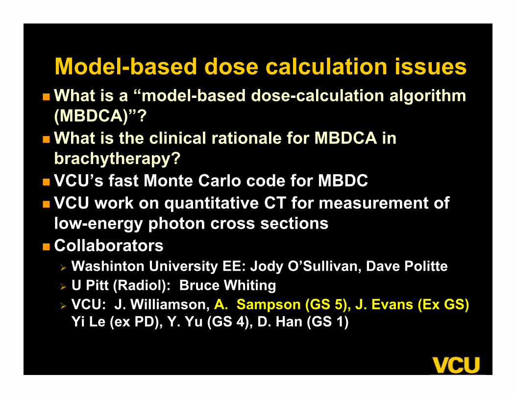
Model-based dose calculation issuesWhat is a “model-based dose-calculation algorithm
(MBDCA)”?What is the clinical rationale for MBDCA in
brachytherapy? VCU’s fast Monte Carlo code for MBDCVCU work on quantitative CT for measurement of
low-energy photon cross sectionsCollaborators
Washinton University EE: Jody O’Sullivan, Dave Politte U Pitt (Radiol): Bruce Whiting VCU: J. Williamson, A. Sampson (GS 5), J. Evans (Ex GS)
Yi Le (ex PD), Y. Yu (GS 4), D. Han (GS 1)
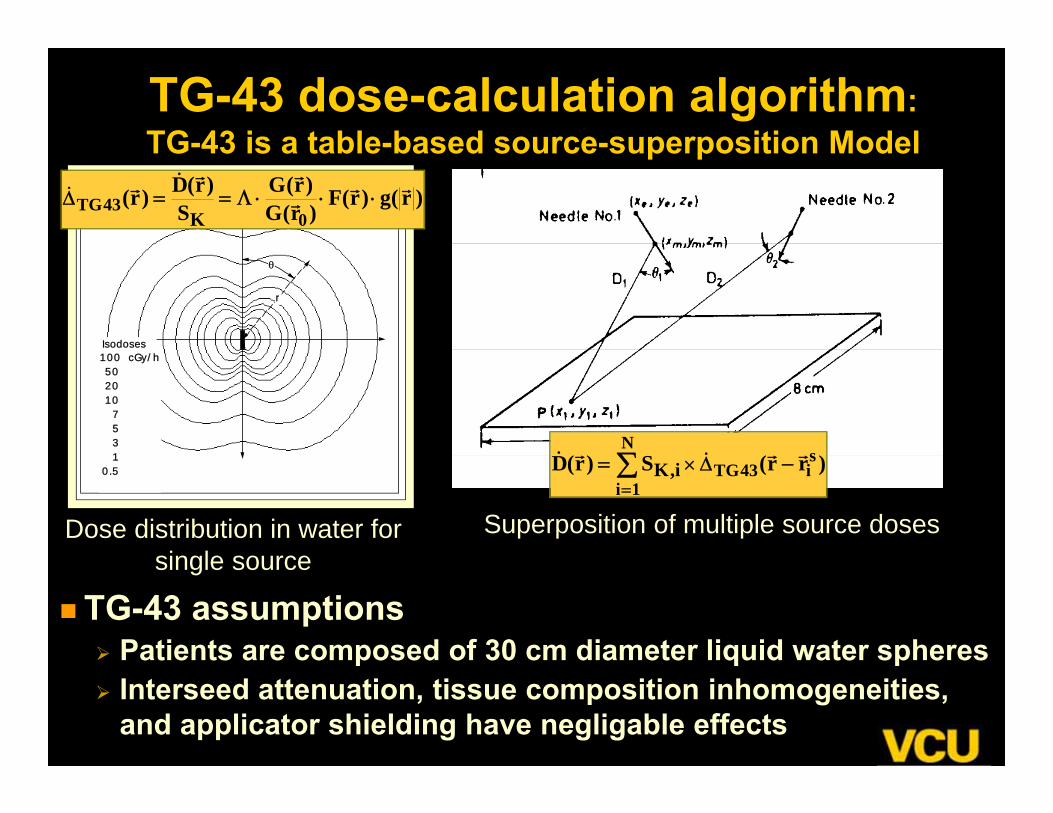
TG-43 dose-calculation algorithm:TG-43 is a table-based source-superposition Model
r
100 cGy/h 50 20 10 7 5 3 1
0.5
Isodoses
Dose distribution in water for single source
Superposition of multiple source doses
TG430K
D(r) G(r)(r) F(r) g( r )S G(r )
Ns
TG43 ii 1
K,iD(r) S (r r )
TG-43 assumptions Patients are composed of 30 cm diameter liquid water spheres Interseed attenuation, tissue composition inhomogeneities,
and applicator shielding have negligable effects
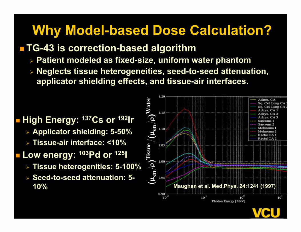
Why Model-based Dose Calculation? TG-43 is correction-based algorithm
Patient modeled as fixed-size, uniform water phantom Neglects tissue heterogeneities, seed-to-seed attenuation,
applicator shielding effects, and tissue-air interfaces.
Maughan et al. Med.Phys. 24:1241 (1997)
High Energy: 137Cs or 192Ir Applicator shielding: 5-50% Tissue-air interface: <10%
Low energy: 103Pd or 125I Tissue heterogenities: 5-100% Seed-to-seed attenuation: 5-
10%
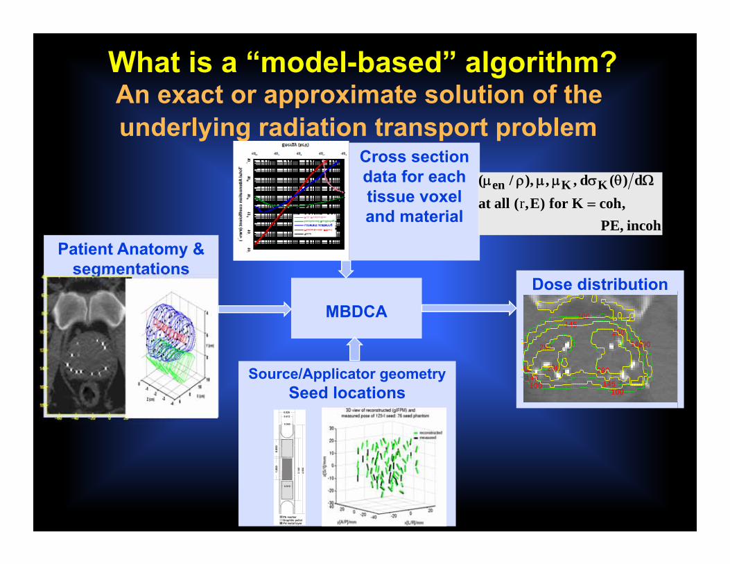
What is a “model-based” algorithm?An exact or approximate solution of the underlying radiation transport problem
Cross section data for each tissue voxel and material
Patient Anatomy & segmentations
Source/Applicator geometrySeed locations
4.50
0
0.826 0.612
3.14
0
0.89
0
0.560
1.09
0
0.510
Graphite pelletPb marker
MBDCADose distribution
100100
100
100
0
145145
145
145
45 290
290
290
290
r
en K K( / ), , , d ( ) d
at all ( ,E) for K coh, PE, incoh
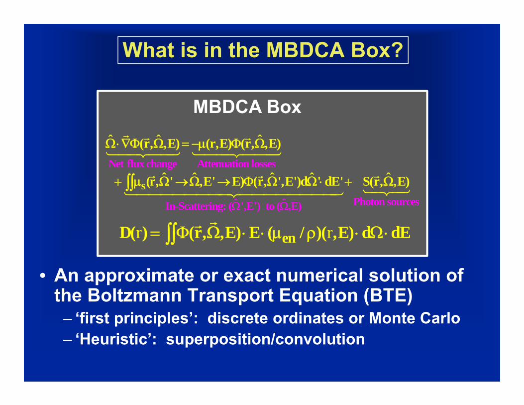
What is in the MBDCA Box?
r r
enD( ) (r, ,E) E ( / )( ,E) d dE
Net flux change Attenuation losses
ˆ ˆIn-Scattering: ( ',E') to
s
(
ˆ ˆ ˆ(r, ,E) (r,E) (r, ,E)
ˆ ˆ ˆ ˆ(r, ' ,E' E) (r, ',E')
d ' dE'
Photon sources,E)
ˆS(r, ,E)
MBDCA Box
• An approximate or exact numerical solution of the Boltzmann Transport Equation (BTE)
– ‘first principles’: discrete ordinates or Monte Carlo– ‘Heuristic’: superposition/convolution
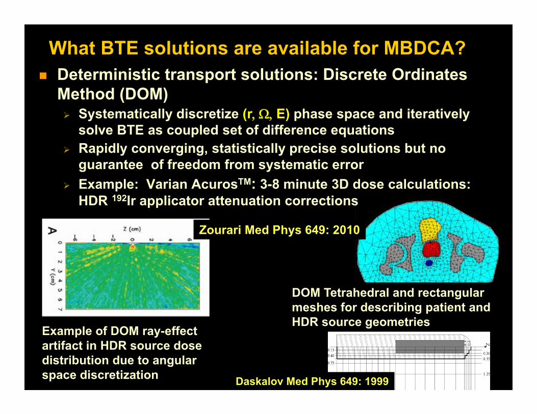
What BTE solutions are available for MBDCA? Deterministic transport solutions: Discrete Ordinates
Method (DOM) Systematically discretize (rE) phase space and iteratively
solve BTE as coupled set of difference equations Rapidly converging, statistically precise solutions but no
guarantee of freedom from systematic error Example: Varian AcurosTM: 3-8 minute 3D dose calculations:
HDR 192Ir applicator attenuation corrections
Example of DOM ray-effect artifact in HDR source dose distribution due to angular space discretization
DOM Tetrahedral and rectangular meshes for describing patient and HDR source geometries
Zourari Med Phys 649: 2010
Daskalov Med Phys 649: 1999
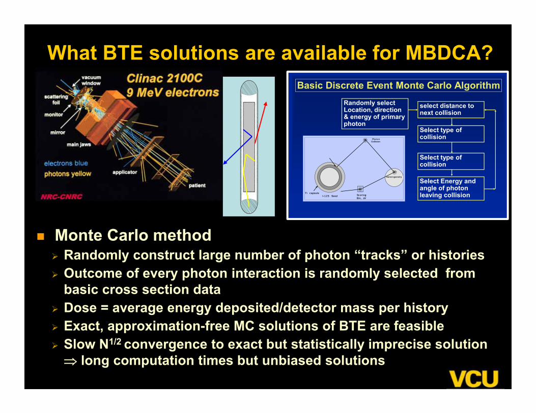
What BTE solutions are available for MBDCA?
Monte Carlo method Randomly construct large number of photon “tracks” or histories Outcome of every photon interaction is randomly selected from
basic cross section data Dose = average energy deposited/detector mass per history Exact, approximation-free MC solutions of BTE are feasible Slow N1/2 convergence to exact but statistically imprecise solution long computation times but unbiased solutions
Basic Discrete Event Monte Carlo Algorithm
select distance to next collision
Randomly select Location, direction & energy of primary photon
Select type of collision
Select type of collision
Select Energy and angle of photon leaving collision
Heterogeneity
Photon Collision
Ti capsuleScor ing Bin, V
I-125 Seed
Ag core
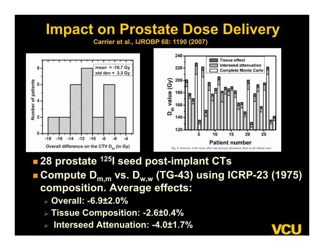
Impact on Prostate Dose Delivery
28 prostate 125I seed post-implant CTsCompute Dm,m vs. Dw,w (TG-43) using ICRP-23 (1975)
composition. Average effects: Overall: -6.9±2.0% Tissue Composition: -2.6±0.4% Interseed Attenuation: -4.0±1.7%
Carrier et al., IJROBP 68: 1190 (2007)
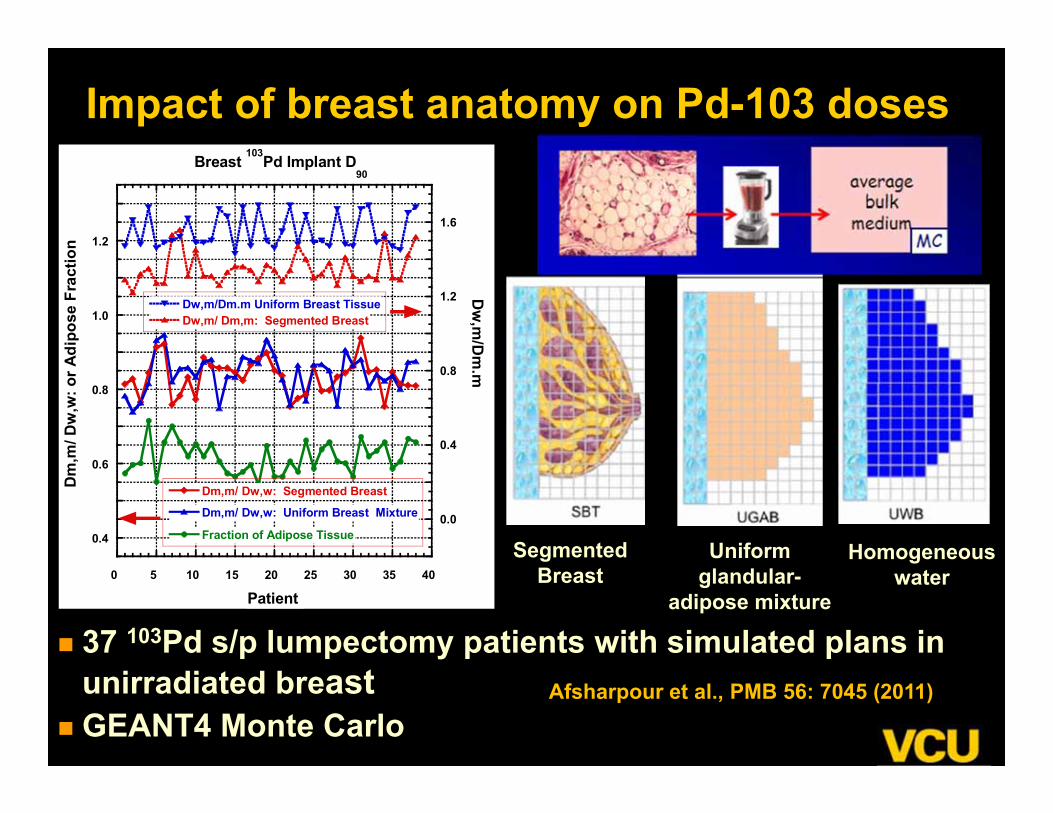
Impact of breast anatomy on Pd-103 doses
37 103Pd s/p lumpectomy patients with simulated plans in unirradiated breast
GEANT4 Monte Carlo
0.4
0.6
0.8
1.0
1.2
0.0
0.4
0.8
1.2
1.6
0 5 10 15 20 25 30 35 40
Breast 103Pd Implant D90
Dm,m/ Dw,w: Segmented Breast
Dm,m/ Dw,w: Uniform Breast Mixture
Fraction of Adipose Tissue
Dw,m/Dm.m Uniform Breast TissueDw,m/ Dm,m: Segmented Breast
Dm
,m/ D
w,w
: or A
dipo
se F
ract
ion
Dw
,m/D
m.m
Patient
Segmented Breast
Uniform glandular-
adipose mixture
Homogeneous water
Afsharpour et al., PMB 56: 7045 (2011)
Novel model-based Dose-Calculation algorithms: VCU work
Super-fast Monte Carlo using correlated sampling
Work of Yi Le (Post doc) and Andrew Sampson (Med. Phys. Ph.D. student)
Sampson, Ye, and Williamson: Med Phys (In Press) 2012Chibani and Williamson: Med Phys 3688: 2005Hedtjarn, Alm-Carlsson, and Williamson: Phys Med Biol 351: 2002

Correlated Sampling concept
Phase space: Precomputed list of single-seed histories transported to seed surface
corrijk het hom
corrcorrijkhet TG43
hom TG43
TG43 TG43
Then Beca
D D (ijk) D (ijk)
D (ijk) D (ijk) DD (ijuse of phase-space source
V
k) D (ijk)
D (ijk) V D (ijk) 0ariance of
corrcorr uncorrijkhet het V D (ijk) V D V D (ijk)
Average dose difference over simulated histories:
If het and het strongly correlated, then
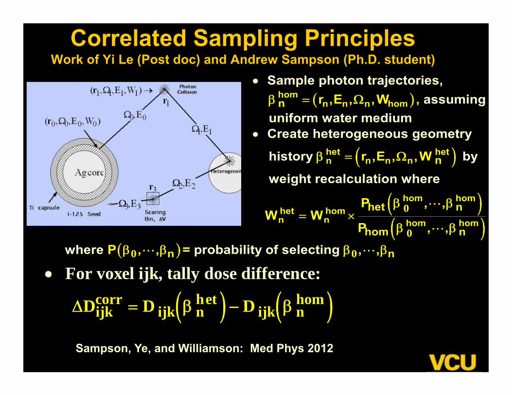
Correlated Sampling PrinciplesWork of Yi Le (Post doc) and Andrew Sampson (Ph.D. student)
homn n n hom
het hetn n n n
hetn
n
n
Sample photon trajectories, assuming
uniform water medium Create heterogeneous geometry
history by
weight recalculation where
r ,E , ,W ,
r ,E , ,W
W
0
0
hom homhomn hom hom
het n
hom n
P , ,W
P , ,
corr het homijk ijk n ijk n
For voxel ijk, tally dose difference:
D D D
Sampson, Ye, and Williamson: Med Phys 2012
0 0 n nwhere probability of selectP , , = i , ,ng
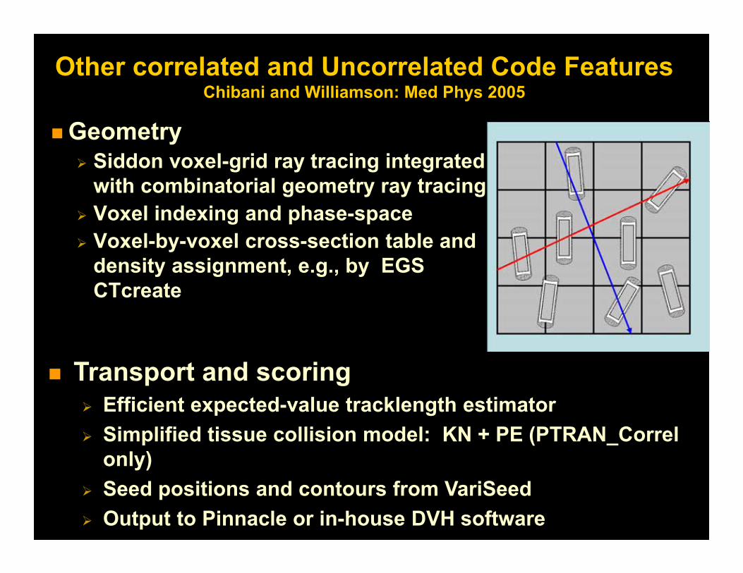
Other correlated and Uncorrelated Code Features Chibani and Williamson: Med Phys 2005
Geometry Siddon voxel-grid ray tracing integrated
with combinatorial geometry ray tracing Voxel indexing and phase-space Voxel-by-voxel cross-section table and
density assignment, e.g., by EGS CTcreate
Transport and scoring Efficient expected-value tracklength estimator Simplified tissue collision model: KN + PE (PTRAN_Correl
only) Seed positions and contours from VariSeed Output to Pinnacle or in-house DVH software
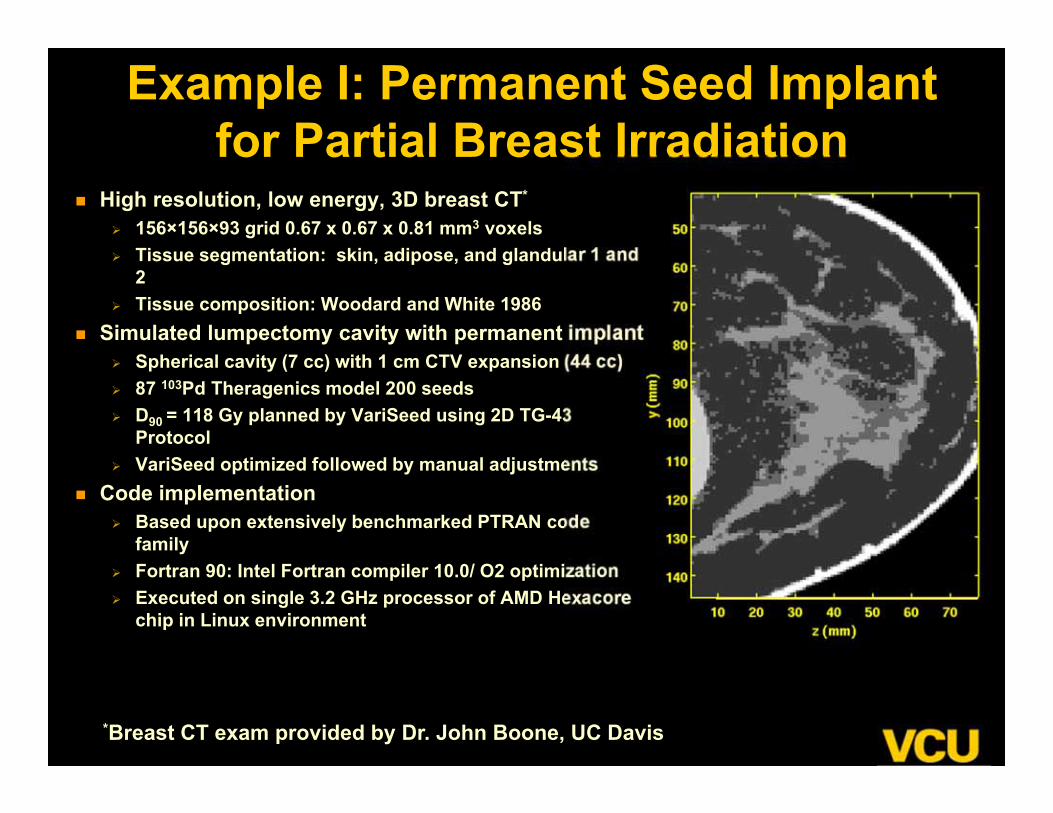
Example I: Permanent Seed Implant for Partial Breast Irradiation
High resolution, low energy, 3D breast CT*
156×156×93 grid 0.67 x 0.67 x 0.81 mm3 voxels Tissue segmentation: skin, adipose, and glandular 1 and
2 Tissue composition: Woodard and White 1986
Simulated lumpectomy cavity with permanent implant Spherical cavity (7 cc) with 1 cm CTV expansion (44 cc) 87 103Pd Theragenics model 200 seeds D90 = 118 Gy planned by VariSeed using 2D TG-43
Protocol VariSeed optimized followed by manual adjustments
Code implementation Based upon extensively benchmarked PTRAN code
family Fortran 90: Intel Fortran compiler 10.0/ O2 optimization Executed on single 3.2 GHz processor of AMD Hexacore
chip in Linux environment
*Breast CT exam provided by Dr. John Boone, UC Davis
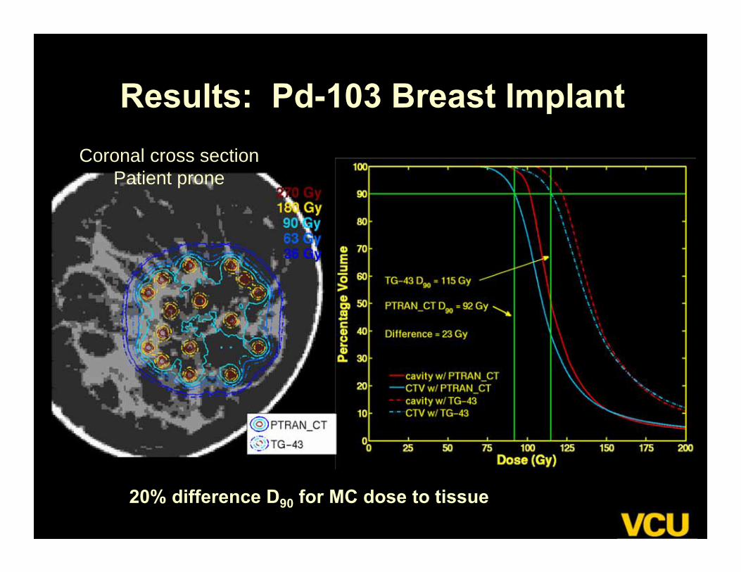
Results: Pd-103 Breast Implant
20% difference D90 for MC dose to tissue
Coronal cross sectionPatient prone
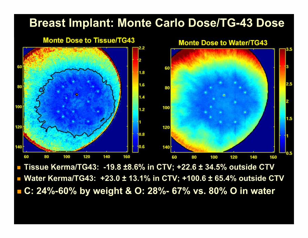
Breast Implant: Monte Carlo Dose/TG-43 Dose
Tissue Kerma/TG43: -19.8 ±8.6% in CTV; +22.6 ± 34.5% outside CTV Water Kerma/TG43: +23.0 ± 13.1% in CTV; +100.6 ± 65.4% outside CTV C: 24%-60% by weight & O: 28%- 67% vs. 80% O in water
Monte Dose to Tissue/TG43 Monte Dose to Water/TG43
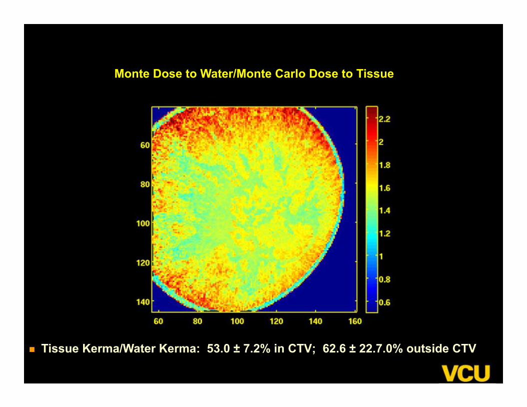
Monte Dose to Water/Monte Carlo Dose to Tissue
Tissue Kerma/Water Kerma: 53.0 ± 7.2% in CTV; 62.6 ± 22.7.0% outside CTV
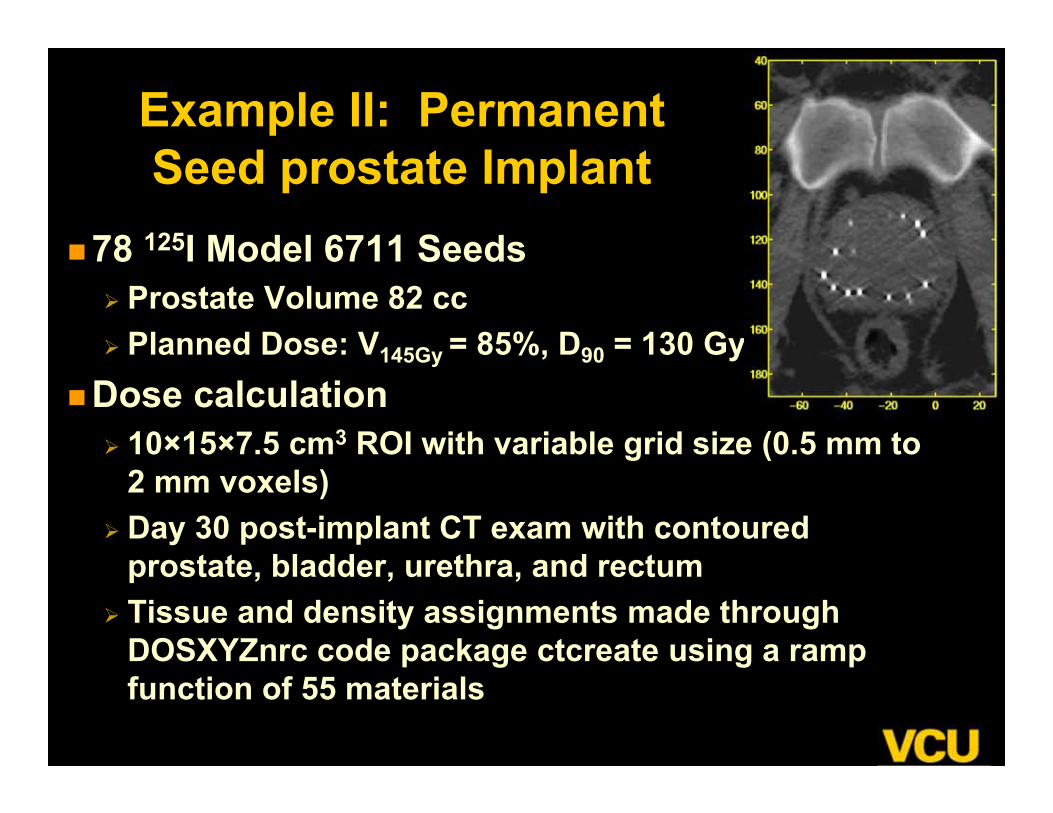
Example II: Permanent Seed prostate Implant
78 125I Model 6711 Seeds Prostate Volume 82 cc Planned Dose: V145Gy = 85%, D90 = 130 Gy
Dose calculation 10×15×7.5 cm3 ROI with variable grid size (0.5 mm to
2 mm voxels) Day 30 post-implant CT exam with contoured
prostate, bladder, urethra, and rectum Tissue and density assignments made through
DOSXYZnrc code package ctcreate using a ramp function of 55 materials
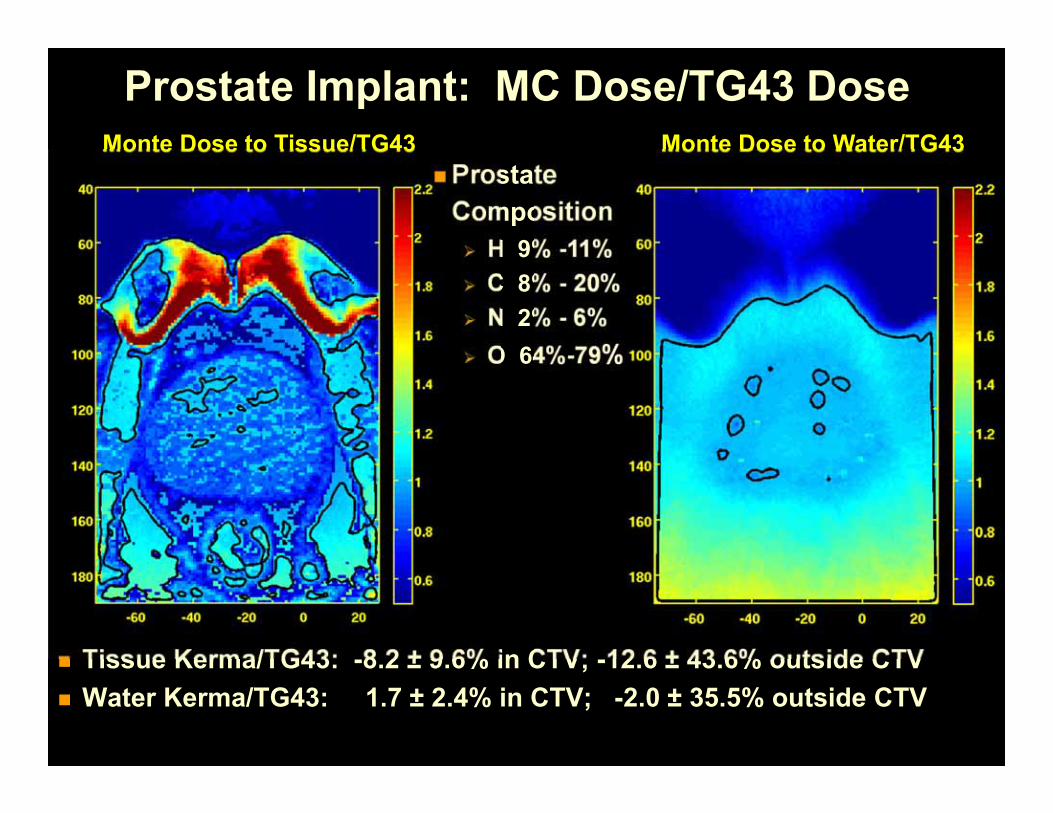
Prostate Implant: MC Dose/TG43 DoseMonte Dose to Tissue/TG43 Monte Dose to Water/TG43
Tissue Kerma/TG43: -8.2 ± 9.6% in CTV; -12.6 ± 43.6% outside CTV Water Kerma/TG43: 1.7 ± 2.4% in CTV; -2.0 ± 35.5% outside CTV
Prostate Composition H 9% -11% C 8% - 20% N 2% - 6% O 64%-79%
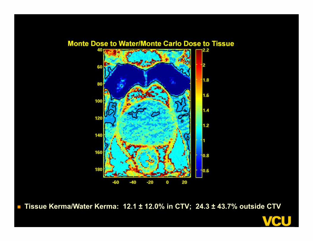
Monte Dose to Water/Monte Carlo Dose to Tissue
Tissue Kerma/Water Kerma: 12.1 ± 12.0% in CTV; 24.3 ± 43.7% outside CTV
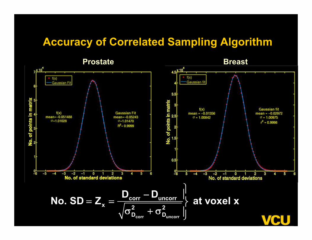
Accuracy of Correlated Sampling Algorithm
corr uncorr
corr uncorrx 2 2
D D
D DNo. SD Z at voxel x
Prostate Breast
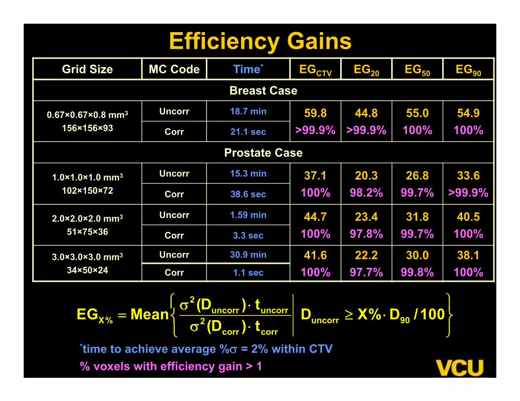
Efficiency GainsGrid Size MC Code Time* EGCTV EG20 EG50 EG90
Breast Case
0.67×0.67×0.8 mm3
156×156×93
Uncorr 18.7 min 59.8>99.9%
44.8>99.9%
55.0100%
54.9100%Corr 21.1 sec
Prostate Case
1.0×1.0×1.0 mm3
102×150×72
Uncorr 15.3 min 37.1100%
20.398.2%
26.899.7%
33.6>99.9%Corr 38.6 sec
2.0×2.0×2.0 mm3
51×75×36
Uncorr 1.59 min 44.7100%
23.497.8%
31.899.7%
40.5100%Corr 3.3 sec
3.0×3.0×3.0 mm3
34×50×24Uncorr 30.9 min 41.6
100%22.2
97.7%30.0
99.8%38.1
100%Corr 1.1 sec
*time to achieve average % = 2% within CTV% voxels with efficiency gain > 1
2uncorr uncorr
X% uncorr 902corr corr
(D ) tEG Mean D X% D /100(D ) t
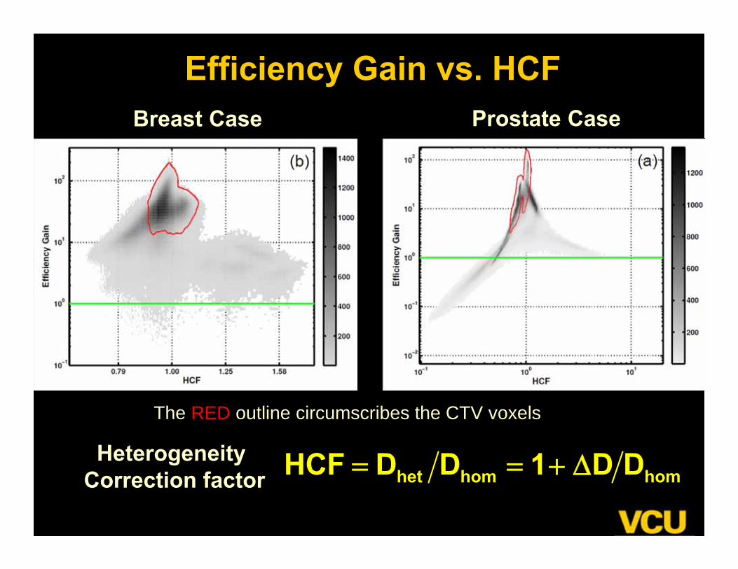
Efficiency Gain vs. HCF
het hom homHCF D D 1 D D
Breast Case Prostate Case
Heterogeneity Correction factor
The RED outline circumscribes the CTV voxels
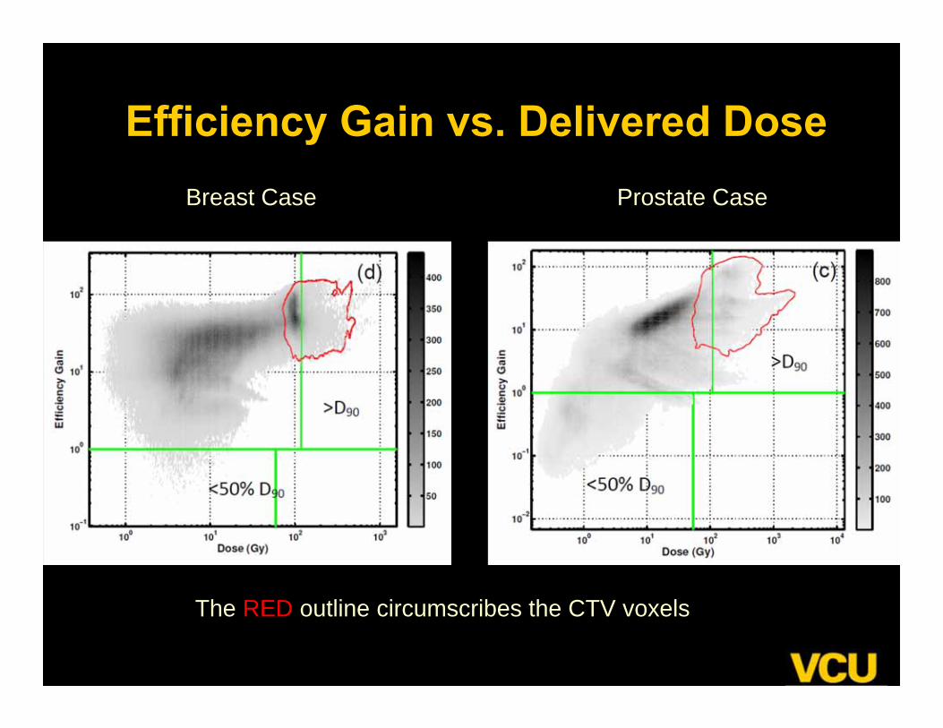
Efficiency Gain vs. Delivered DoseBreast Case Prostate Case
The RED outline circumscribes the CTV voxels
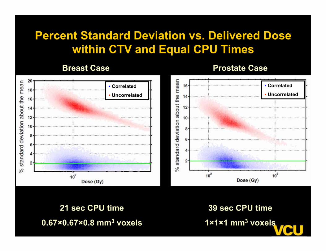
Percent Standard Deviation vs. Delivered Dose within CTV and Equal CPU Times
Breast Case Prostate Case
21 sec CPU time
0.67×0.67×0.8 mm3 voxels
39 sec CPU time
1×1×1 mm3 voxels
• Correlated
• Uncorrelated• Correlated
• Uncorrelated
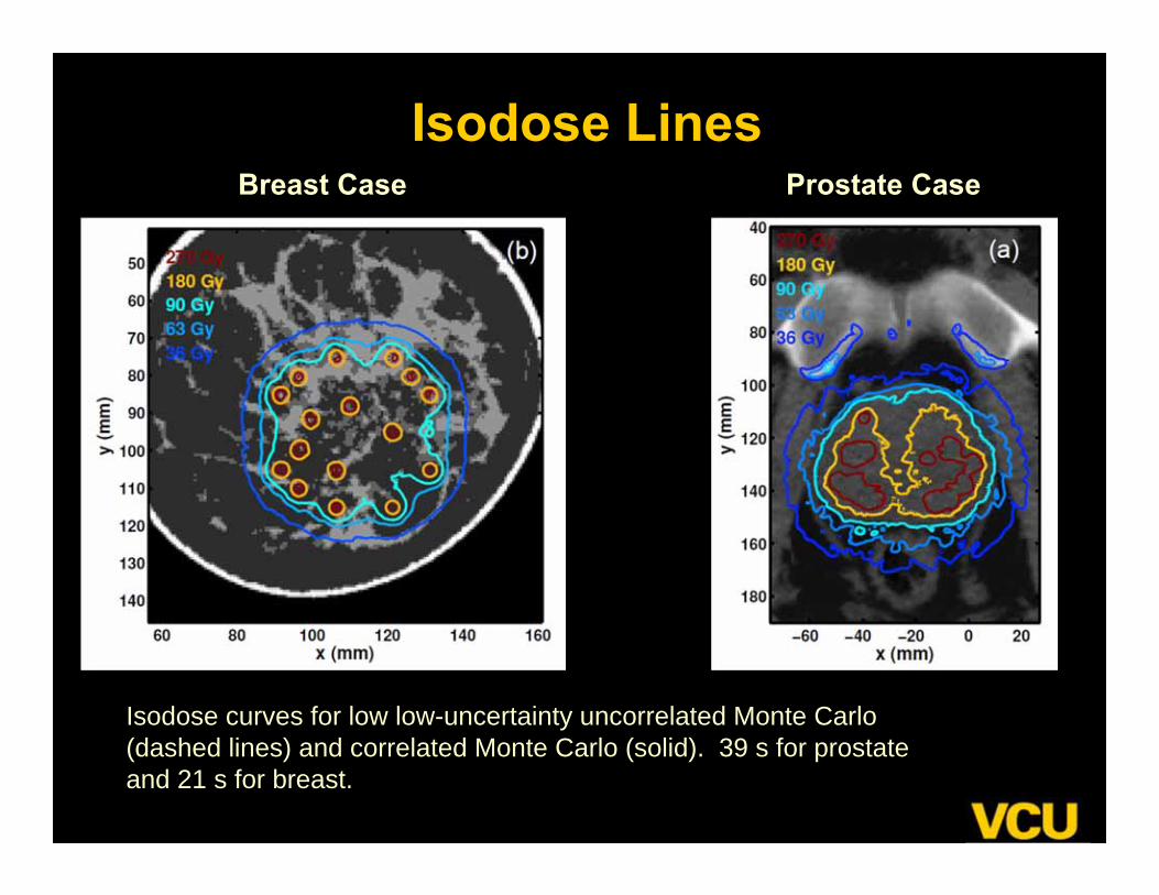
Isodose LinesBreast Case Prostate Case
Isodose curves for low low-uncertainty uncorrelated Monte Carlo (dashed lines) and correlated Monte Carlo (solid). 39 s for prostate and 21 s for breast.
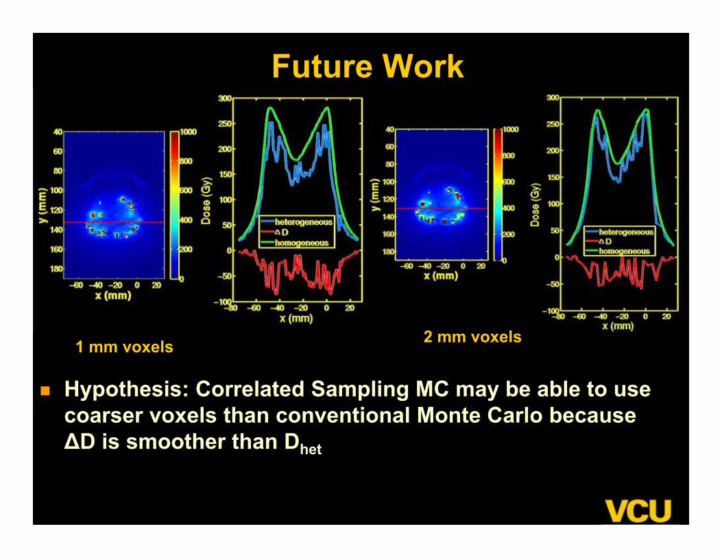
Future Work
2 mm voxels
Hypothesis: Correlated Sampling MC may be able to use coarser voxels than conventional Monte Carlo because ΔD is smoother than Dhet
1 mm voxels
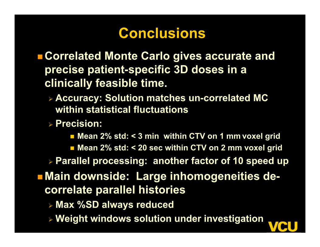
ConclusionsCorrelated Monte Carlo gives accurate and
precise patient-specific 3D doses in a clinically feasible time. Accuracy: Solution matches un-correlated MC
within statistical fluctuations Precision:
Mean 2% std: < 3 min within CTV on 1 mm voxel grid Mean 2% std: < 20 sec within CTV on 2 mm voxel grid
Parallel processing: another factor of 10 speed upMain downside: Large inhomogeneities de-
correlate parallel histories Max %SD always reduced Weight windows solution under investigation
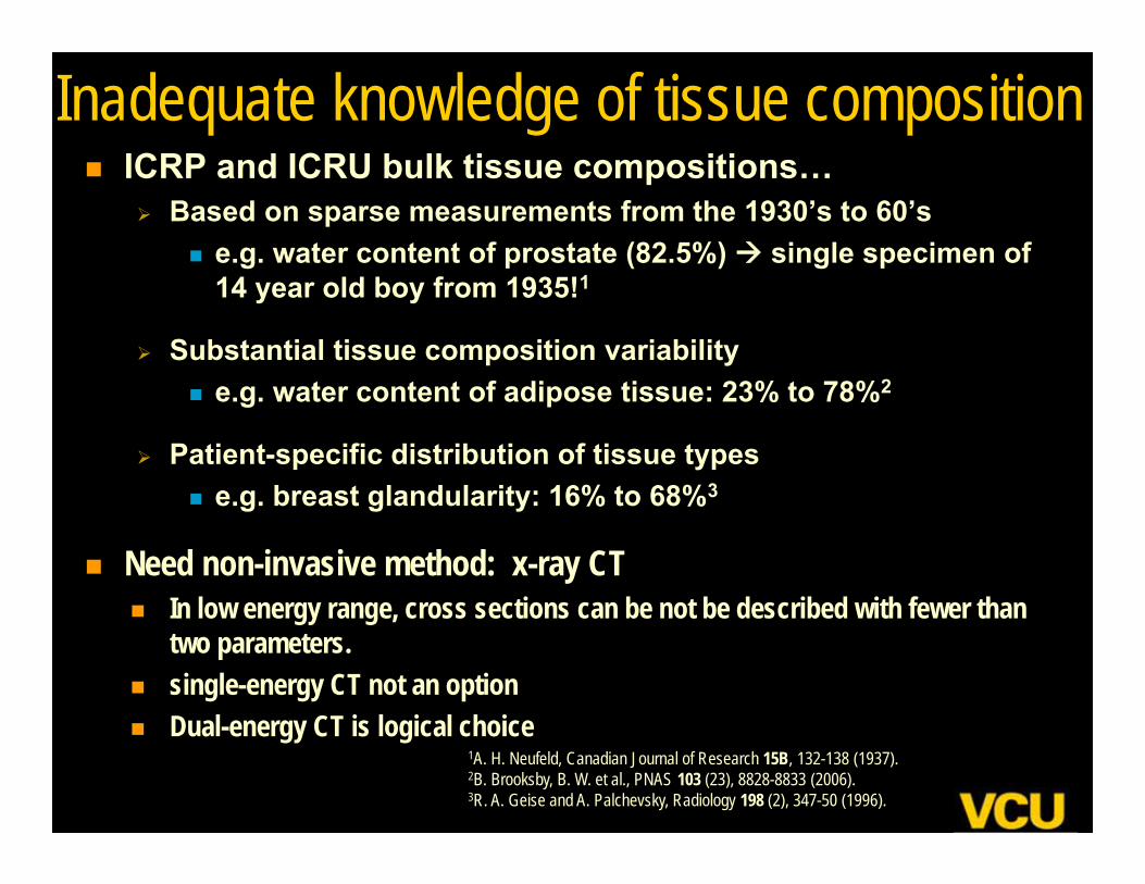
Inadequate knowledge of tissue composition ICRP and ICRU bulk tissue compositions…
Based on sparse measurements from the 1930’s to 60’s e.g. water content of prostate (82.5%) single specimen of
14 year old boy from 1935!1
Substantial tissue composition variability e.g. water content of adipose tissue: 23% to 78%2
Patient-specific distribution of tissue types e.g. breast glandularity: 16% to 68%3
Need non-invasive method: x-ray CT In low energy range, cross sections can be not be described with fewer than
two parameters. single-energy CT not an option Dual-energy CT is logical choice
1A. H. Neufeld, Canadian Journal of Research 15B, 132-138 (1937).2B. Brooksby, B. W. et al., PNAS 103 (23), 8828-8833 (2006).3R. A. Geise and A. Palchevsky, Radiology 198 (2), 347-50 (1996).
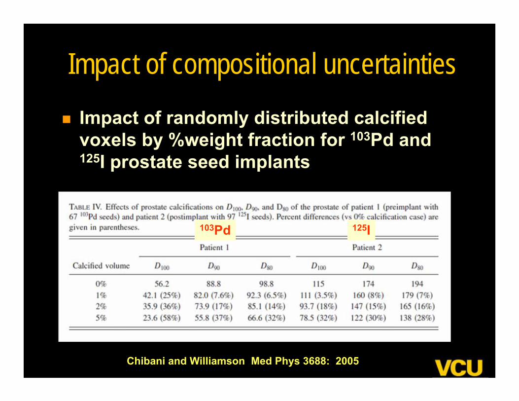
Impact of compositional uncertainties Impact of randomly distributed calcified
voxels by %weight fraction for 103Pd and 125I prostate seed implants
103Pd 125I
Chibani and Williamson Med Phys 3688: 2005
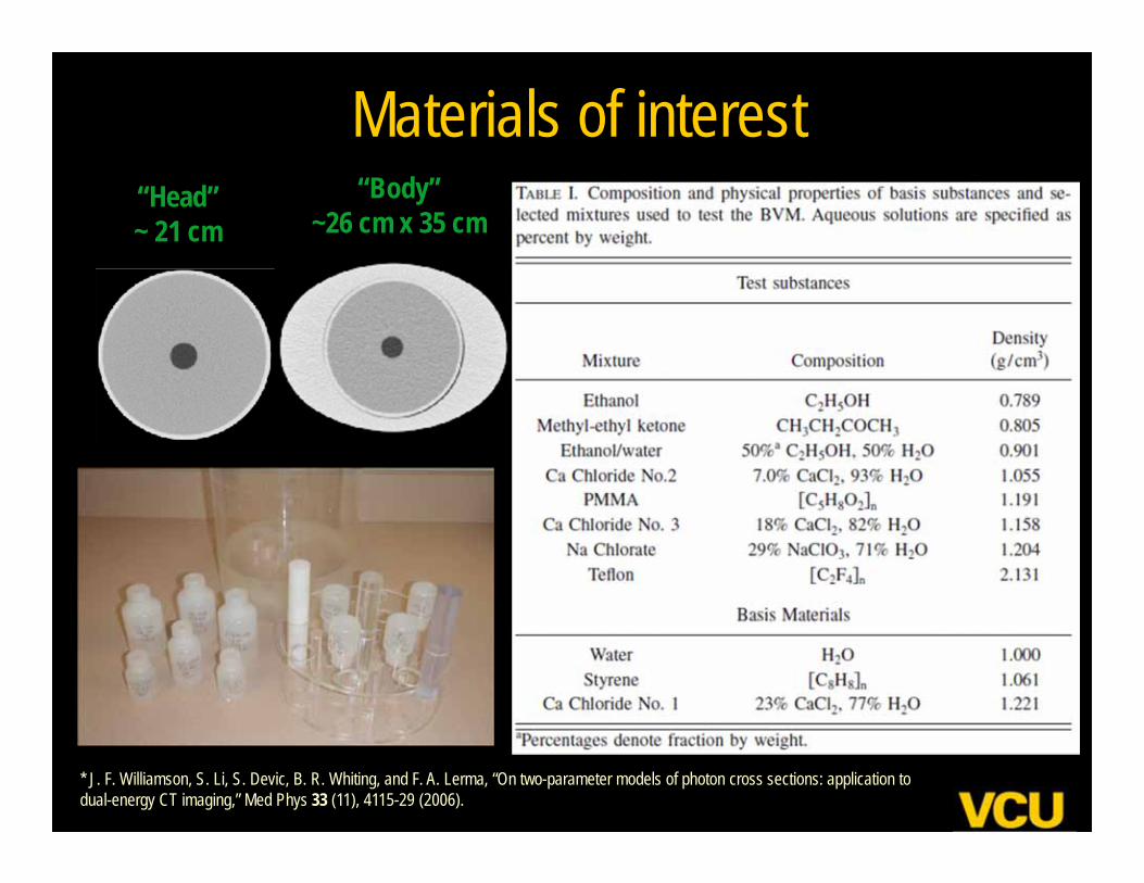
Materials of interest
* J. F. Williamson, S. Li, S. Devic, B. R. Whiting, and F. A. Lerma, “On two-parameter models of photon cross sections: application to dual-energy CT imaging,” Med Phys 33 (11), 4115-29 (2006).
“Body”~26 cm x 35 cm
“Head”~ 21 cm
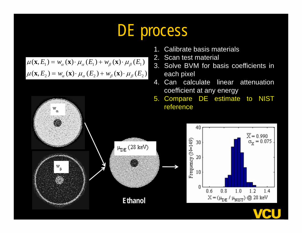
DE process1. Calibrate basis materials2. Scan test material3. Solve BVM for basis coefficients in
each pixel4. Can calculate linear attenuation
coefficient at any energy5. Compare DE estimate to NIST
reference
1 1 1
2 2 2
( , ) ( ) ( ) ( ) ( )
( , ) ( ) ( ) ( ) ( )
x x x
x x x
E w E w E
E w E w E
Ethanol
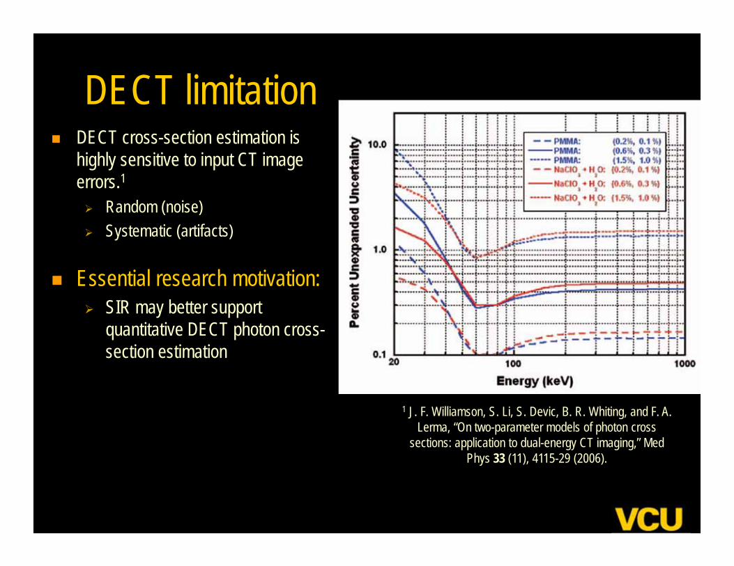
DECT limitation DECT cross-section estimation is
highly sensitive to input CT image errors.1 Random (noise) Systematic (artifacts)
Essential research motivation: SIR may better support
quantitative DECT photon cross-section estimation
1 J. F. Williamson, S. Li, S. Devic, B. R. Whiting, and F. A. Lerma, “On two-parameter models of photon cross
sections: application to dual-energy CT imaging,” Med Phys 33 (11), 4115-29 (2006).
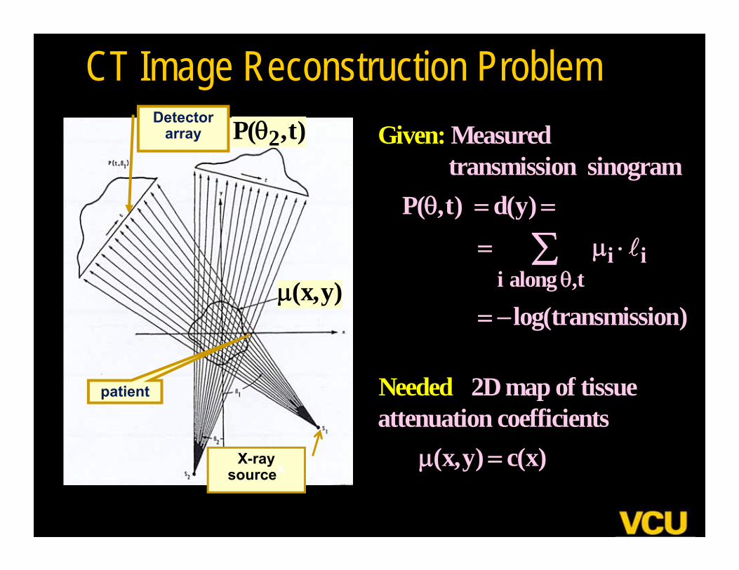
CT Image Reconstruction Problem
X-ray sourcex
Detector array
i ii along ,t
Measured transmission sinogram P( ,t) d(y)
log(transmission)
2D map of tissue attenuation coefficien
Given:
Neets
: ded
(x,y ) c(x)
patient
(x,y)
2P( ,t)
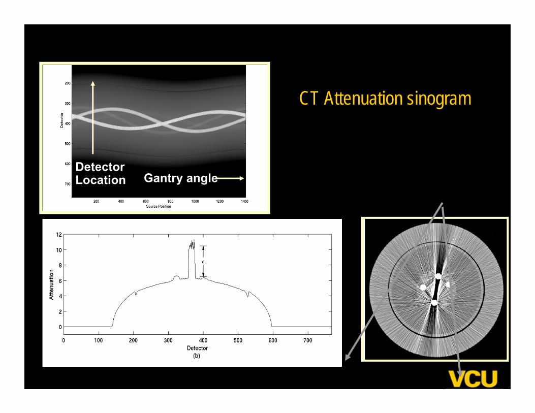
CT Attenuation sinogram
Gantry angleDetectorLocation
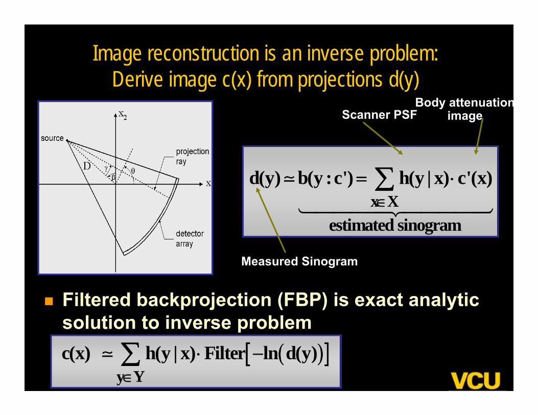
Image reconstruction is an inverse problem: Derive image c(x) from projections d(y)
Filtered backprojection (FBP) is exact analytic solution to inverse problem
x Xestimated sinogram
d(y) b(y :c') h(y | x) c'(x)
Scanner PSFBody attenuation
image
Measured Sinogram
y Y
c(x) h(y | x) Filter ln d(y)
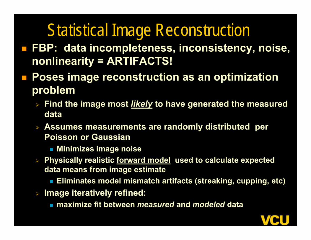
Statistical Image Reconstruction FBP: data incompleteness, inconsistency, noise,
nonlinearity = ARTIFACTS! Poses image reconstruction as an optimization
problem Find the image most likely to have generated the measured
data Assumes measurements are randomly distributed per
Poisson or Gaussian Minimizes image noise
Physically realistic forward model used to calculate expected data means from image estimate Eliminates model mismatch artifacts (streaking, cupping, etc)
Image iteratively refined: maximize fit between measured and modeled data
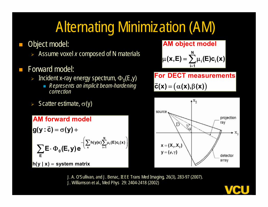
Alternating Minimization (AM) Object model:
Assume voxel x composed of N materials
Forward model: Incident x-ray energy spectrum, 0(E,y)
Represents an implicit beam-hardening correction
Scatter estimate, (y)
N
i ix i 1
h(y|x) (E)c (x)
0E
h(y | x) system matrix
g(AM forward
y : c)m
(y)
E (E,y)e
odel
N
i ii 1
(x,
AM object
E) (E)c
model
(x)
J. A. O'Sullivan, and J. Benac, IEEE Trans Med Imaging, 26(3), 283-97 (2007).J. Williamson et al., Med Phys 29: 2404-2418 (2002)
For DECT measuremenc(x)
ts(x), (x)
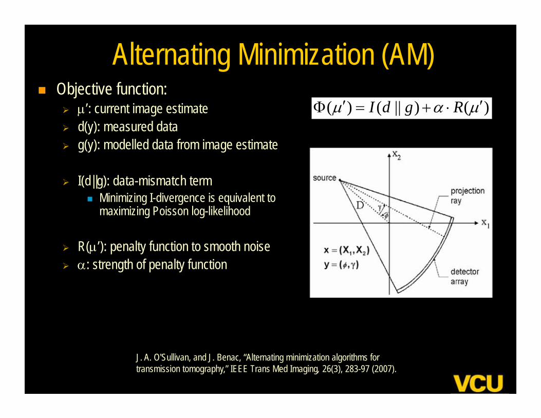
Alternating Minimization (AM) Objective function:
’: current image estimate d(y): measured data g(y): modelled data from image estimate
I(d||g): data-mismatch term Minimizing I-divergence is equivalent to
maximizing Poisson log-likelihood
R(’): penalty function to smooth noise : strength of penalty function
( ) ( || ) ( )I d g R
J. A. O'Sullivan, and J. Benac, “Alternating minimization algorithms for transmission tomography,” IEEE Trans Med Imaging, 26(3), 283-97 (2007).
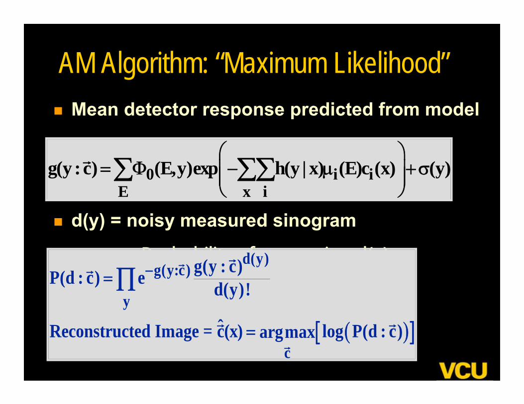
AM Algorithm: “Maximum Likelihood” Mean detector response predicted from model
d(y) = noisy measured sinogram
Probability of measuring d(y)
0 i iE x i
g(y :c) (E,y)exp h(y | x) (E)c (x) (y)
d(y)g(y:c)
y
c
g(y : c)P(d : c) e d(y)!
ˆReconstructed Image = c(x) log P(d : c)argmax
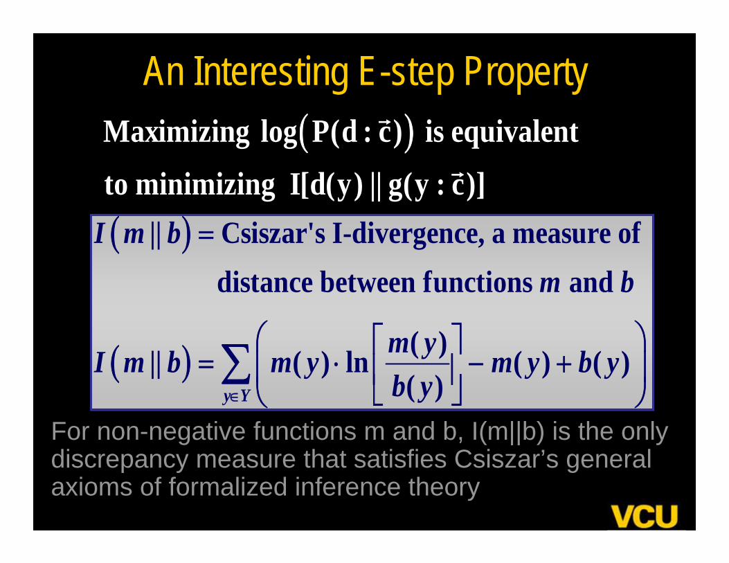
An Interesting E-step Property
For non-negative functions m and b, I(m||b) is the only discrepancy measure that satisfies Csiszar’s general axioms of formalized inference theory
Maximizing log P(d : c) is equivalentto minimizing I[d(y) || g(y : c)]
|| Csiszar's I-divergence, a measure of distance between functions and
( )|| ( ) ln ( ) ( )( )y Y
I m bm b
m yI m b m y m y b yb y
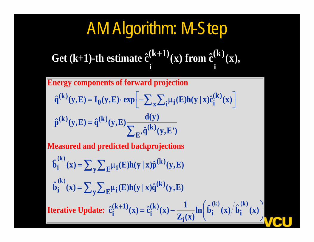
AM Algorithm: M-Step
(k )
(k)(k)0 i ix i
(k) (k)(k)
E'
(k)i i
ˆ ˆq (y,E) I (y,E) exp (E)h(y | x)c (x)
d(y)ˆ ˆp (y,
Energy components of forward projection
Measured and predicted backprojections
E) q (y,E)q (y,E')
ˆb (x) (E)h(y | x)p (y
(k )
(k) (k)
y E
(k)i iy E
(k 1) (k)i ii i
iIterative Update
,E)
ˆ ˆb (x) (E)h(y | x)q (y,E)
1 ˆˆ ˆc (x) c (x) ln b (x) b (x)Z (x)
:
i i(k 1) (k)ˆ ˆGet (k+1)-th estimate c (x) from c (x),
Iterative E-M reconstruction: FBP alternative
Can incorporate realistic detector model into FP operation that includes nonlinear detector behavior
More robust: will generate best image in presence of incomplete or inconsistent data
Can constrain image formation process using a priori knowledge, e.g., known shape, composition of metal rods
Drawback: very computationally intensive
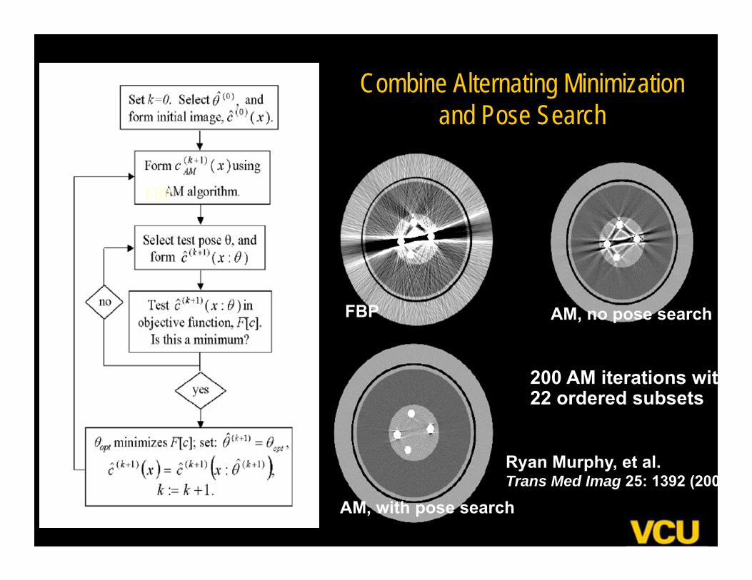
Combine Alternating Minimizationand Pose Search
FBP
FBP
AM, no pose search
AM, with pose search
200 AM iterations wit22 ordered subsets
Ryan Murphy, et al.Trans Med Imag 25: 1392 (200
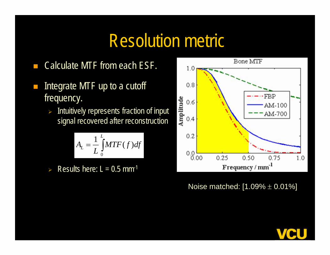
Resolution metric Calculate MTF from each ESF.
Integrate MTF up to a cutoff frequency. Intuitively represents fraction of input
signal recovered after reconstruction
Results here: L = 0.5 mm-1
0
1 ( )L
LA MTF f dfL
Noise matched: [1.09% 0.01%]
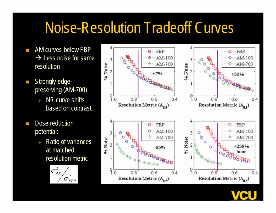
Noise-Resolution Tradeoff Curves AM curves below FBP Less noise for same resolution
Strongly edge-preserving (AM-700) NR curve shifts
based on contrast
Dose reduction potential: Ratio of variances
at matched resolution metric
2
2AM
FBP
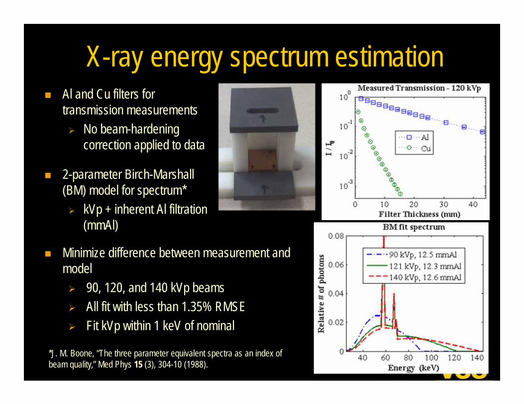
X-ray energy spectrum estimation Al and Cu filters for
transmission measurements No beam-hardening
correction applied to data
2-parameter Birch-Marshall (BM) model for spectrum* kVp + inherent Al filtration
(mmAl)
*J. M. Boone, “The three parameter equivalent spectra as an index of beam quality,” Med Phys 15 (3), 304-10 (1988).
Minimize difference between measurement and model 90, 120, and 140 kVp beams All fit with less than 1.35% RMSE Fit kVp within 1 keV of nominal
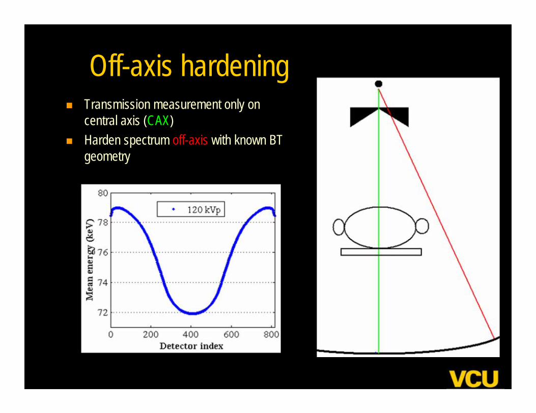
Off-axis hardening Transmission measurement only on
central axis (CAX) Harden spectrum off-axis with known BT
geometry
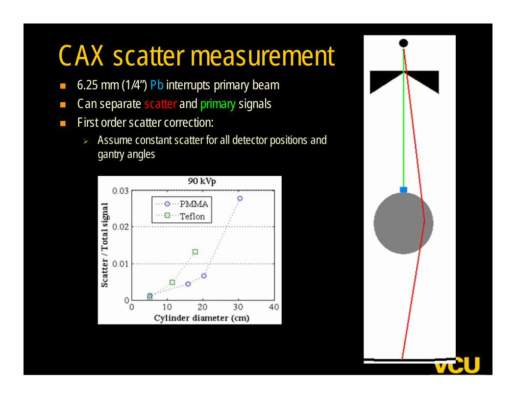
CAX scatter measurement 6.25 mm (1/4”) Pb interrupts primary beam Can separate scatter and primary signals First order scatter correction:
Assume constant scatter for all detector positions and gantry angles
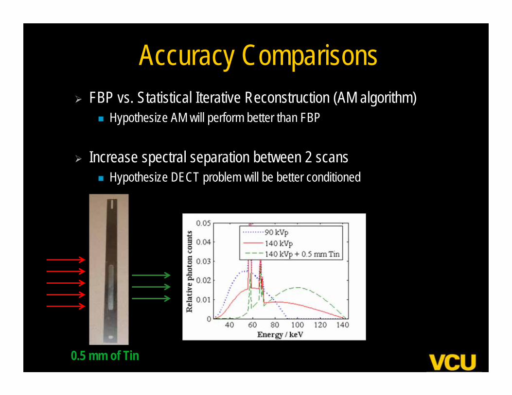
Accuracy Comparisons FBP vs. Statistical Iterative Reconstruction (AM algorithm)
Hypothesize AM will perform better than FBP
Increase spectral separation between 2 scans Hypothesize DECT problem will be better conditioned
0.5 mm of Tin
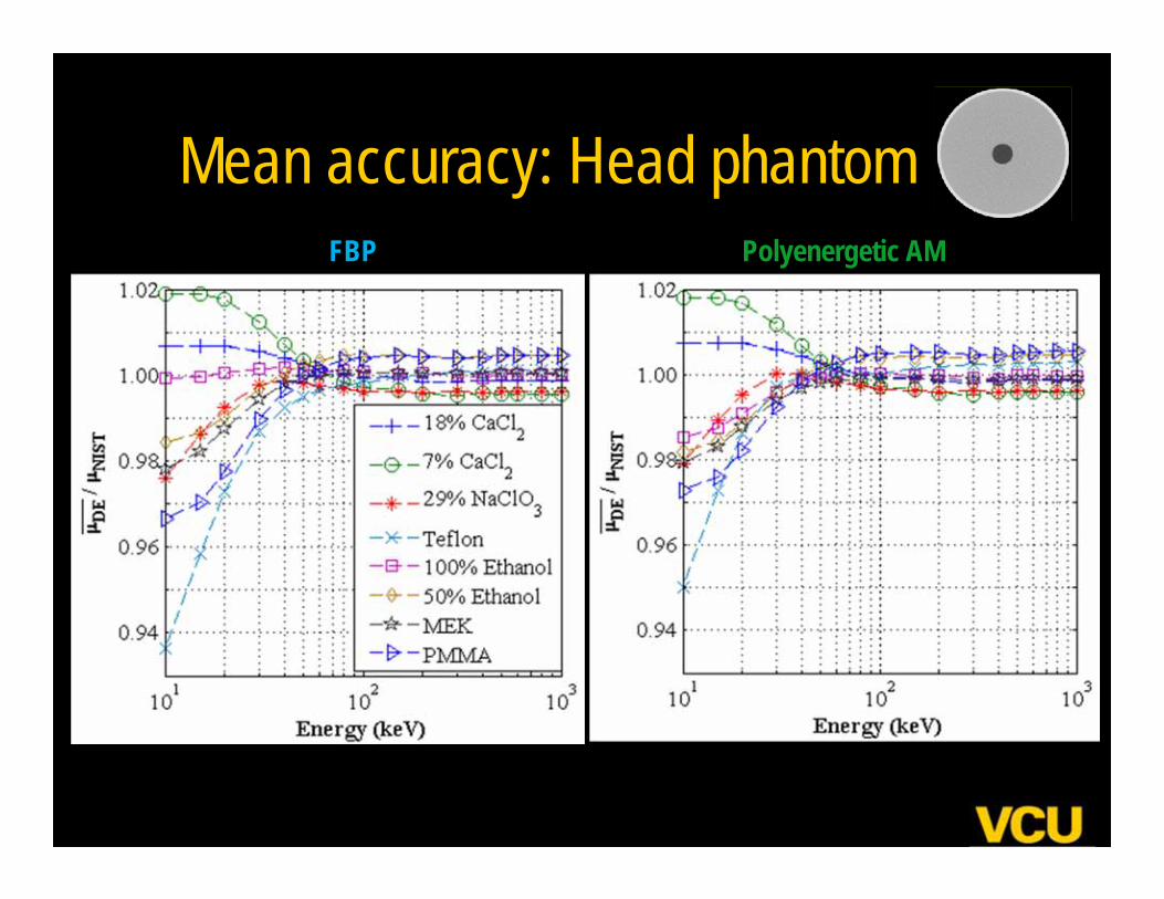
Mean accuracy: Head phantomPolyenergetic AMFBP
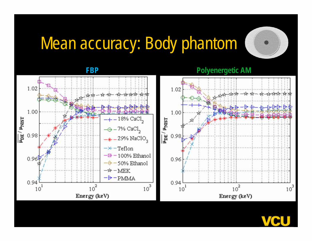
Mean accuracy: Body phantomPolyenergetic AMFBP
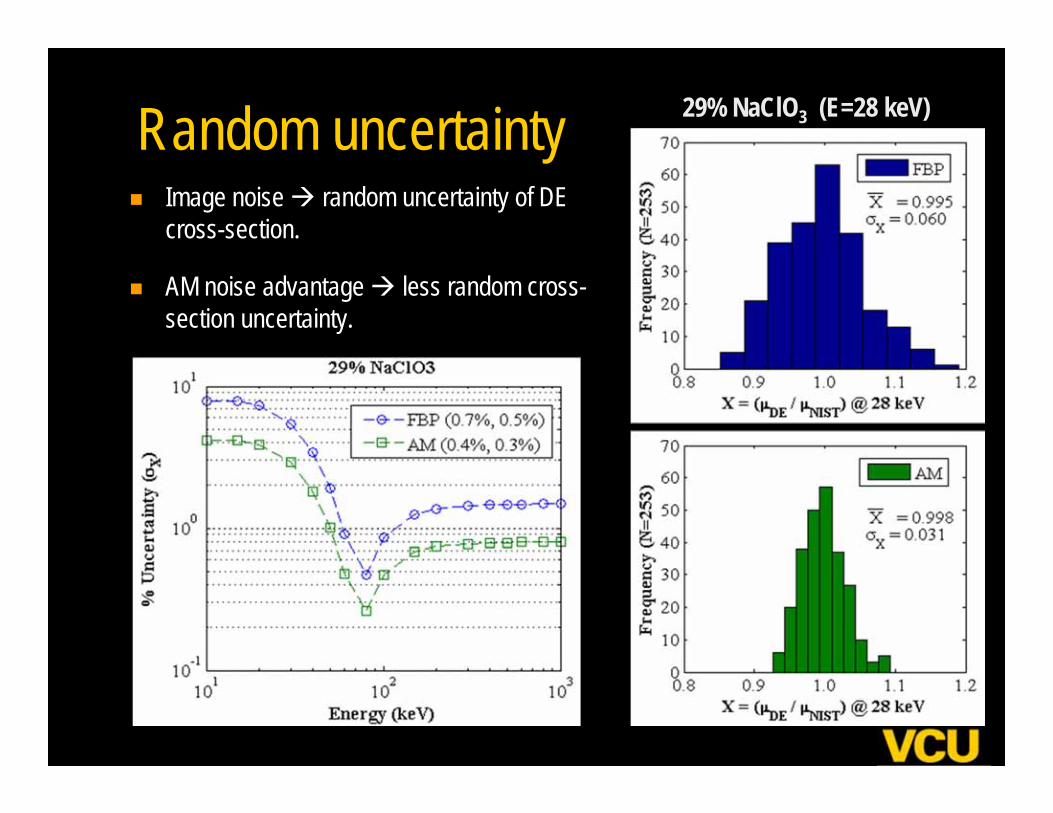
Random uncertainty Image noise random uncertainty of DE
cross-section.
AM noise advantage less random cross-section uncertainty.
29% NaClO3 (E=28 keV)
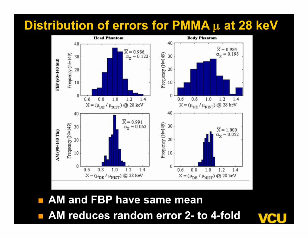
Distribution of errors for PMMA at 28 keV
AM and FBP have same mean AM reduces random error 2- to 4-fold
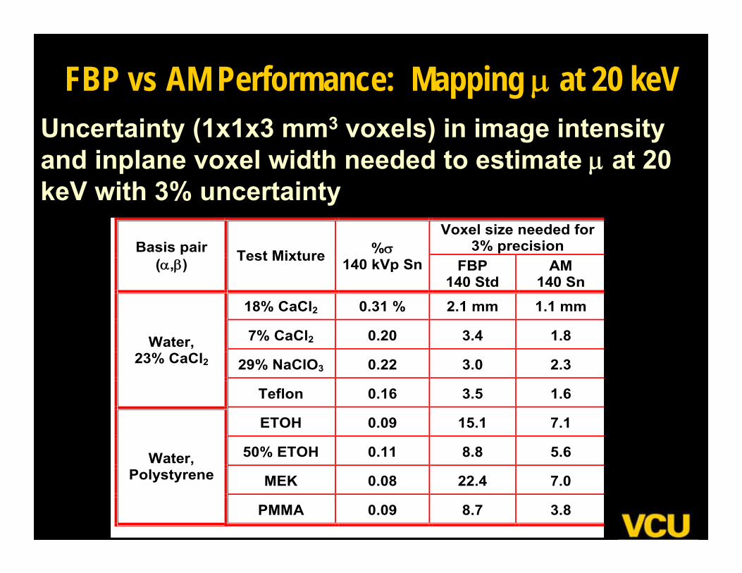
FBP vs AM Performance: Mapping at 20 keV Uncertainty (1x1x3 mm3 voxels) in image intensity and inplane voxel width needed to estimate at 20 keV with 3% uncertainty
Basis pair (,) Test Mixture %
140 kVp Sn
Voxel size needed for 3% precision
FBP140 Std
AM140 Sn
Water, 23% CaCl2
18% CaCl2 0.31 % 2.1 mm 1.1 mm
7% CaCl2 0.20 3.4 1.8
29% NaClO3 0.22 3.0 2.3
Teflon 0.16 3.5 1.6
Water, Polystyrene
ETOH 0.09 15.1 7.1
50% ETOH 0.11 8.8 5.6
MEK 0.08 22.4 7.0
PMMA 0.09 8.7 3.8
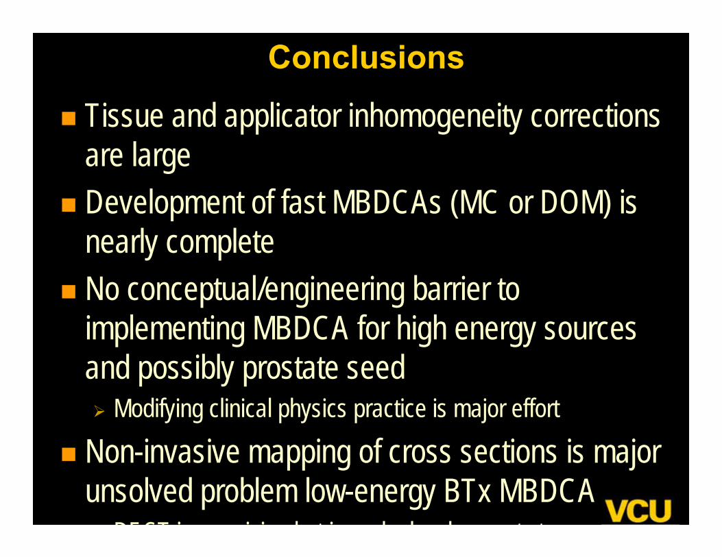
Conclusions
Tissue and applicator inhomogeneity corrections are large
Development of fast MBDCAs (MC or DOM) is nearly complete
No conceptual/engineering barrier to implementing MBDCA for high energy sources and possibly prostate seed Modifying clinical physics practice is major effort
Non-invasive mapping of cross sections is major unsolved problem low-energy BTx MBDCA
DECT i i i b t i l d l t t
Virginia Commonwealth University
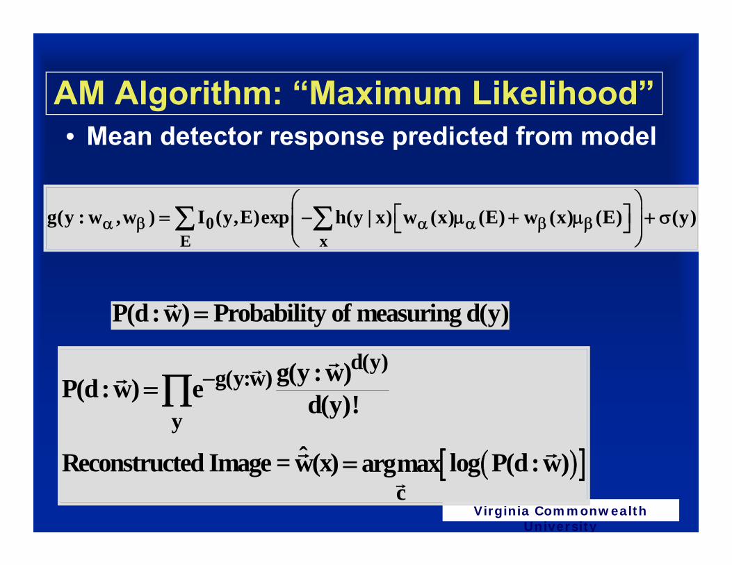
AM Algorithm: “Maximum Likelihood”• Mean detector response predicted from model
• d(y) = noisy measured sinogram
0E x
g(y : w ,w ) I (y,E)exp h(y | x) w (x) (E) w (x) (E) (y)
d(y)g(y:w)
y
c
g(y :w)P(d:w) e d(y)!
ˆReconstructed Image = w(x) log P(d:w)argmax
P(d:w) Probability of measuring d(y)
Virginia Commonwealth University
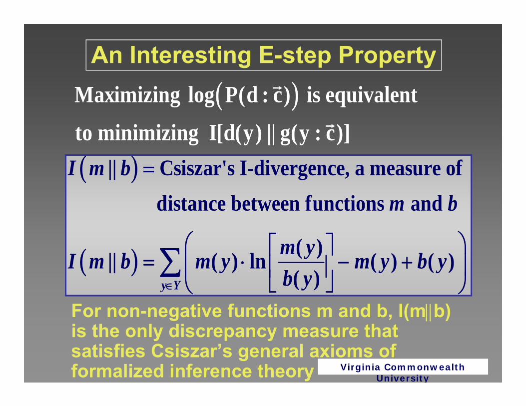
An Interesting E-step Property
For non-negative functions m and b, I(mb) is the only discrepancy measure that satisfies Csiszar’s general axioms of formalized inference theory
Maximizing log P(d : c) is equivalentto minimizing I[d(y) || g(y : c)]
|| Csiszar's I-divergence, a measure of distance between functions and
( )|| ( ) ln ( ) ( )( )y Y
I m bm b
m yI m b m y m y b yb y
Virginia Commonwealth University
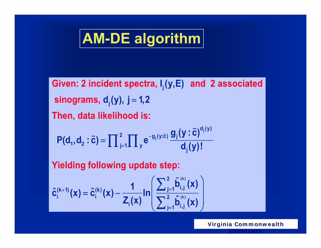
AM-DE algorithm
j
j
j
j
d (y)2 g (y:c) j
1 2 j 1 yj
(k 1)i
Given: 2 incident spectra, and 2 associated sinograms, Then, data likelihood
I (y,E)d (y), j 1,2
g (y : c)
P(d ,d : c) e d (y)!
is:
Yielding following update ste
ˆ c
p:
(k )
(k )
2i, jj 1(k)
i 2i i, jj 1
b (x)1ˆ(x) c (x) ln ˆZ (x) b (x)
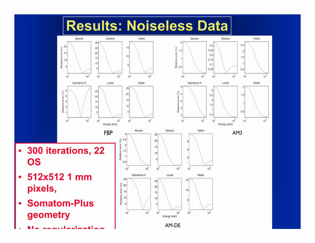
Results: Noiseless Data
• 300 iterations, 22 OS
• 512x512 1 mm pixels,
• Somatom-Plus geometry
• No regularization
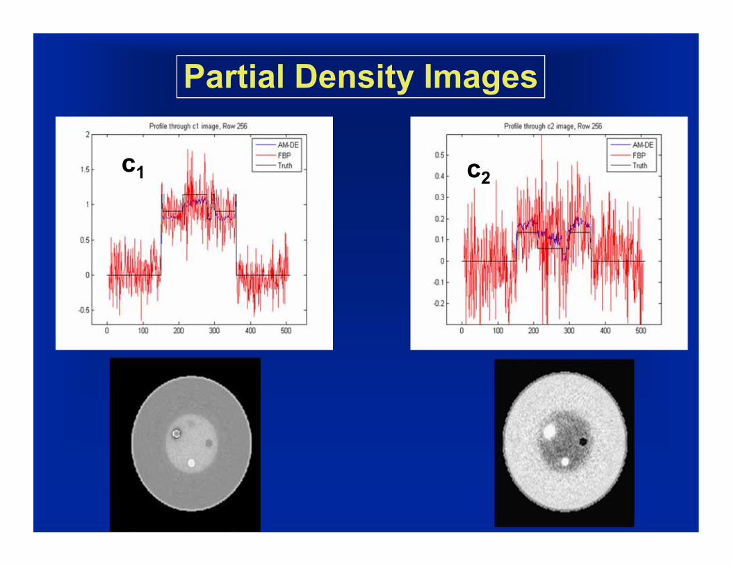
Partial Density Images
• nc1 c2
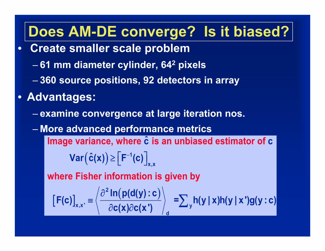
Does AM-DE converge? Is it biased?• Create smaller scale problem
– 61 mm diameter cylinder, 642 pixels– 360 source positions, 92 detectors in array
• Advantages: – examine convergence at large iteration nos.– More advanced performance metrics
1x,x
2
x,x ' yd
Image variance, where is an unbiased estimator of
where
c cˆ Var c(x) F (c)
ln p(d(y) : c
Fisher informa
F(c) = h(y | x)h(y | x ')g(y : c
tion is given
)
by
c(x) c(x ')
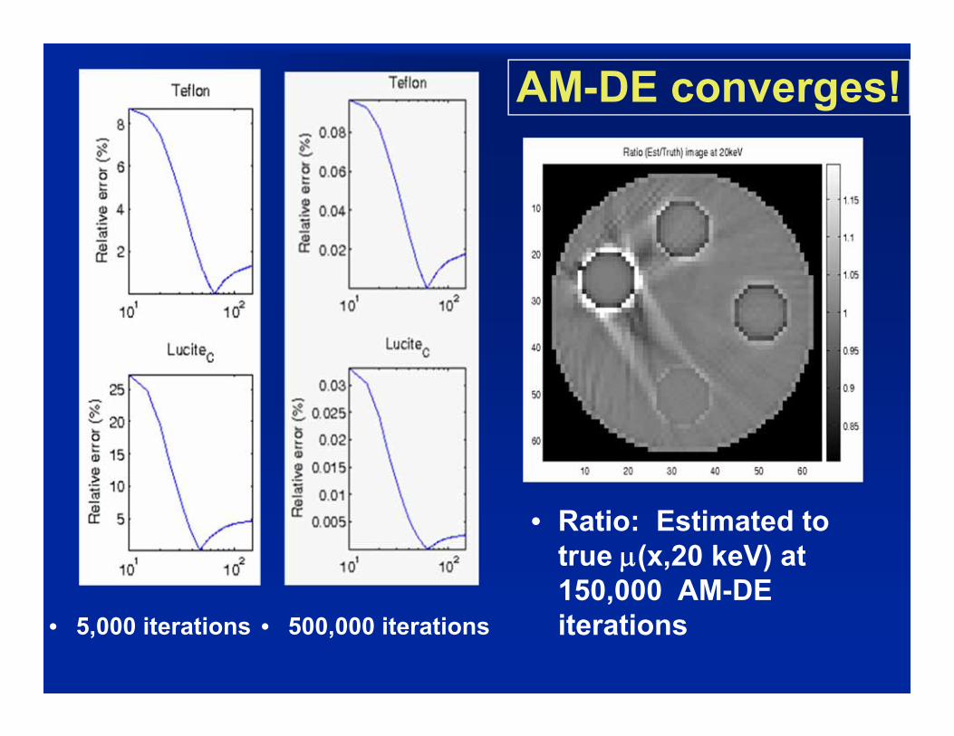
AM-DE converges!
• 5,000 iterations • 500,000 iterations
• Ratio: Estimated to true (x,20 keV) at 150,000 AM-DE iterations
Virginia Commonwealth University
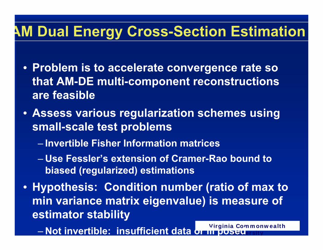
AM Dual Energy Cross-Section Estimation
• Problem is to accelerate convergence rate so that AM-DE multi-component reconstructions are feasible
• Assess various regularization schemes using small-scale test problems
– Invertible Fisher Information matrices– Use Fessler’s extension of Cramer-Rao bound to
biased (regularized) estimations
• Hypothesis: Condition number (ratio of max to min variance matrix eigenvalue) is measure of estimator stability
– Not invertible: insufficient data or ill posed
Virginia Commonwealth University
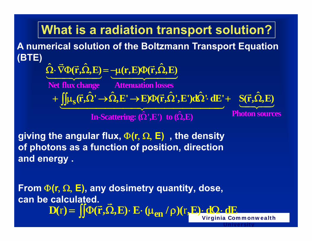
What is a radiation transport solution?
giving the angular flux, (rE) , the density of photons as a function of position, direction and energy .
From (rE), any dosimetry quantity, dose, can be calculated.
r r
enD( ) (r, ,E) E ( / )( ,E) d dE
Net flux change Attenuation losses
ˆ ˆIn-Scattering: ( ',E') to
s
(
ˆ ˆ ˆ(r, ,E) (r,E) (r, ,E)
ˆ ˆ ˆ ˆ(r, ' ,E' E) (r, ',E')
d ' dE'
Photon sources,E)
ˆS(r, ,E)
A numerical solution of the Boltzmann Transport Equation (BTE)
Virginia Commonwealth University
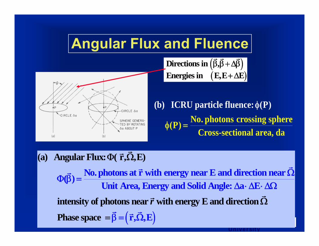
Angular Flux and Fluence
Directions in ,Energies in E,E E
No. photon(b) ICR
s crossinU particle fluence
g sphere(P)Cross-section
: (P)
al area, da
No. photons at r with energy near E and direction near( )Unit
(a) Angular Flux: ( r, ,E)
intensity of photons nAre
eara, Energy and So
with enerl
gid Angle:
y E and dE
eca
irr
tion
Phase r, space ,E


![RAYSTATION DOSE CALCULATION ALGORITHMS · Dose calculation: RayStation uses the VMC++ [11] code for the in-patient dose calculation. The VMC++ code is optimized for three- dimensional](https://img.pdfslide.us/doc/110x75/5c6577f809d3f29b6e8cc8af/raystation-dose-calculation-algorithms-dose-calculation-raystation-uses-the.jpg)