Embed Size (px)
Citation preview
Electron arc therapy dose calculation using
the angle-P concept.
Pierre Courteau
Medical Physics Unit
McGill University, Montreal
March 1993
A Thesis submitted to
the Faculty of Graduate Studies and Research
in partial fulfillmcnt of the requirements
of the degrce of Mastcr's in
Medical Radiation Physics.
© Pierre Courteau 1993
Il
CONTENTS
Abstract 1 \'
Résumé v
Acknowledgments \'1
1. General introduction
2. Electron arc therapy
2.1 Single electron beams
2.1.1 General
2.1,2 Oblique incidencp.
2.2 Physical properties of arc clectron beams
2.2.1 Beam collimation
2.2.2 Pseudo-arc technique
li
(i
(i
9
1 1
Il
J(j
2.2.3 Effect of bcam parameters on pcrcenlage depth doses 17
2.3 Pencil beams in electron arc therapy 20
2.3.1 Angular spread in air and virtual source position 21
2.3.2 Fermi-Eyges theory Œpreading in medium) 2fi
2.3.3 Summation of pcncIl beams 27
2.3.4 Correction for loss of electrons 2~)
a.
4.
5.
:2.;Ui Use of CT numbers
:2 :3 (j Electron-arc pencil beam algorithm
The angle r~ concept in electron arc therapy
3.1 Physical aspect
:3.2 Isodosc distribution calculation algorithm
Evaluation of the angle ~ conce;>t
<1 1 Introduction
4.2 rnput data
4.2.1 Angle ~ algorithm input data
4.2.2 Pencil beam algorithm input data
4.3 Evaluation
4.3.1 Peucil beam calculation
4.3.2 Measurements with film
4.3.3 Humanoid phantom
Conclusions
References
111
29
31
33
33
44
52
52
52
52
57
59
59
62
68
70
73
A computer T o~ !'
calculate electron arl.-
IV
Abstract
,It'd durlIlg t Il(' rOllt'~e or t 11I~ work to
1:, ons wüh Uw ;lI1~~ll\ I~ (,OIIl'l'pt 'l'I\('
angle ~ uniquely describes i' ..l prndence of raùial pt'rt'l'Ilt a~~(' (kpt Il
doses in electron arc therapy on the nominal field W1dth, I~()<.'l'lltl'r d!'pth,
and virlual source-axis dlstance. 'l'he p concppt. C:1Il lw USI't! III dilllcai
situations ta determinl! the field width wheI1 the lSOl'l'ntl'l" clepth alld tll<'
required radial pel'ccntage depth dose are knOWII 'J'llls thl'sis presl'Ilt S .Ill
overview of the physical properties of electroll arc therapy alld d!':-.rnhl's III
detail the angle p pseudo-arc teehI1lque uscd at. McC:ill. A descrrpt.loll or the algorithms used in the computer program ifS g1ven and the I~ t(I('hniquC'
is cümpared tü measurements and other caiculation l11l'thods.
v
Résumé
Un programme d'ordInateur a été conçu pour calculer les
chstribullOl1S de dose pour des traitements rotationels avec électrons en
ulilisanl Il' concept de l'angle 13. L'angle p décrit la dépendence du
n'miL'ment radial de do:::e en profondeur de façon unique avec la largeur du
champ de radwlion (w), la profondeur de l'isocentre (d) , et la distance
source virtuclll' Ù lsocentre m. Cet angle peut ètre utilIsé dans des
~itualions cliniques pour détermmer w lorsque d et le rendement de dose
en profondeur sont connus. Ce travail présente premièrement une revue
des propnétés physiques de la thérapie rotationelle avec électrons et
ensuite le concC'pt de l'angle P utilisé à McGill est décrit en détail. Les
algorithmes utilisées dans le logiciel de calcul de dose sont aussi
présentées ct finalement la technique dE. thérapie avec l'angle pest
comparée avec des mesures et une autre methode de calcul.
VI
Ackno\vledgments
l would like to thank Dr C, Pla for his help during t hl:-; :>t lld~' .Inti 1'01'
introducing me to programming the ApplC' Maclnto~h (,Ol1lputt"', 1\11'~ 1\1
Pla for sbaring ber knowledge in eledroll arc lI1f'rapy, 1\1 l' 1\1 1':V,IIl~ lil!'
his technical help using the water phantom beam nnaly/.l'1', and. (,Vl't'y
member of the medical physics depart.n1l'nt l'or thl' stlIlllll.ltlll~~
environment,
l also would like to thank my colleaguc Pat. Cadnwl1 t'or his
friendship which made my stay in Montreal a little l('ss palllfui. Alld
finally, many thanks to Nancy for her patIence and for 1)(\1111~ a grp:1I
mother to our girls while l was away,
The financial support which made my studies at McCtll THlsslhlc
was provided by the Dr, Georges-L, Dumont Hospital.
Chapter 1
General introduction
1
There exbt several radiation modalities used ln the treatment of
tum(Jr~ or reglons containing tumor cells. Sm::.lll accessible turnors c::m be
treated by 1 nserting encapsulated radIOactive sources in the [orm of
needles or wires withlO the tumor Othcr lesions accessible from a cavity
may a1so be trcated u~i ng brachytherapy whcre the sources arc placed
against the Il'SlOnS Tlus modality has the advantage of delivering high
d(}:-, .. )~ to the reg"IOI1 of ('onC'crn while efficleIltly ~paring healthy
surrounding ti:-,sues. For the case of deeply seated lesions, combinations of
high cnergy photoll beam~, most often produccd by Cobalt-GO sources or
lincar accell'rators with encrgws of 4 to 25 MeV, are used. Electron beams
with C'nergICs ranging from 4 to 25 MeV are uscd to treat regions that
l'X tend from Lhl' skin surface up to depths of 1 to 8 cm depending on the
(,Ilcrgy. Their !110st common applications arc in the treatrncnt of skin and
lip cancers, chcst wall irradiation for brcast cancer, delivering boost dose
Ln !1odcs, and in the treatment of head and neck cancers. For small
supcrficial lcsions x-rays produccd by potential difTerences of 50 kV to 300
kV are used l'requcntly.
'l'ills work \vill l'ocus on electron arc therapy or rotational electron
ther~py whieh is t he technique of choice in the treatment of certain large
Supt'rticial tUlllors locatcd along curved surfaces, su ch as post-mastectomy
chest wall Ill]. ThIS modality surpasses stationary photon or electron
tipld::\ [7, 15luscd to irradwte large curved areas, due ta the dose
inhomogcnelty \vhich would be produced at the abutment regions of the
•
multiple fields which givcs risc Lo cold and hot ,pot~ EIl'ctron an' tlH'l".\p\',
being a rotat.lOnal elcctron bC<lIll techIllqUt'. may lw pl'rf'ol'Il1cd \\'1 t Il a
continuou~ rotation or by a series of overlapPlng lil'hb dl,It\'l'll,tt III ;111
lsocentric manner at regular angular interval~ (p~l'lldoarT 1:\1)
ThIS technique has been devcloped and llSl'd \Vit h :-'Ul'l'l'S:-' hy \'a["JOll:-'
radiothcrnpy dcpartmcnts but electroll arT t.hl'rapy l'l'tn~llns a clllllpltr,\h'd
and time-consuming technique, therpfore not \Vldl'Iv U:-;l',j 1 t \\'a~. fir'st
described by Becker and Wcitzcl in HHj() [11 Wlt Il a tt'chniqlll' kl\(I\V1\ ;\S
"shell irradiation" usmg elcctrons of les~ than lG l\ll'V l'rom :1 f'J\.t'd
isocenter betatron. Using a \VIde range of el1l'rgws (10 tn ·I:~ M(,V) :d:-;o
pro::luced by a fixed lsoccnter hctatron, Ras!'>()w (1 ~172) [~·t 1 d(,~ct'll)(,d slll:tll
angle penduluIll therapy and Its numernus chl1ll'al 'lpplic;\l.i()l1~
There are severnl factors afTL'cting thl' do~e <hst.ribullOll in pl('('/ rOll
arc therapy making thi8 technique unique, sllch as 1.11(' fi('ld wl(lt.h,
isocenter depth, source to axis distance, e!pdrol1 lH'am (lJlprg'Y, slld'acl'
curvature of the patient, bC~lIn collimatioJl (prilllal'y, SI'('oIH!:Iry !llid
tertiary), and the number of monitor units per degn'(' for COl1ti'llllJlIS arc,
or per bearn for pseudoarc, Khan et aL. [121 ~tlldJed the f'fr(>l't~> of' titI'
isocenter depth and field size on the shape of the radwl I)('f'(·('Ilt.a~(l d('pth
dose curve in order to develop a technique for routine cIlTlIcal US(! wit.h 1:~
MeV electrons, They round that the surf:lce dm,p d('cnJa~('s : III d t.lt:! t Uw
depth of maXImum dose mcreases with lI1creasing- II-oo('('ntpr dppt Il, jlJld Uw
sarne effects are observed when decrea~ing the field width They :d~o round
that skin collimation provides a sharper dose fall'ofT than wh!,l1 no
shielding is used. Ruegseggcr et al. [251 also stud i cd the~(! dfects and wJl,h
the use of a variable isocenter machine (4f) MeV heliltrOn) round t.h:!t t.h(·
parameter responsible for the change ln ~hape of the depth dose eurv(:
3
with ch:mg"lng i~ocenter depth, was the SSD (source-to-skin distance)
wll/ch varie~ dircctly with the isocenter depth for a fixed source-axis
di:..,tallCü. This pfTect cun be explained by looking at the time a point spends
III th(~ h(~;lIll as a funct.ion of isocentpr depth or SSD. The Lime lTIcreases
wiLh UH' distance from the source therefore shifting dma" toward the
isocprllpr They uls\) round an obhqUlty cfTect WhlCh Shlfts dma\: toward the
surf.lce wlH'n tJll' i~occnter depth is rcduccd. this chdnge is in the opposite
direction of the SSD cfTpct, \vhence depending on the paramct.ers, dma ..: can
('ither he larger or smaller than the dma\: for the fixed field. Boyer ct al. [3]
dl'llloIl:,tr:ttpd the f'ca~lbility of a p:..,cudoarc technique employing multiple
ovprlapplllg statlOllury fields which allows elcctron arc therapy to be done
without having to make Cd~tly modificatlOl1S to the linear <.lccelerator.
With tilt' prClpel' choice oC the trcatment paramcters the dose distribution
fllf the pseudoarc doc . ..; Bot difTer from the continuous arc distribution, but
the trp:ttment time to ohtain the E>ume delivcred dose is sorncwhat largcr.
A t.rl'atnll'nt planning mode! for electron arc has been developed by
Leavi tt. et al. [lG 1 \\'here they calculat.e the dose tü a point due ta the arc by
the SUmlllatlOIl of tïxed fields supl~rimposed ln fixed angular Increments
around the arc Hogstrom et al. [6] modified the pencil-beam algorithm for
fixed fields Ln calcuiaLe the dose distrIbution f(lr arc beanls tü reduce the
computatIOn time tu acceptablp levels. This algorithm treats the total arc
as a s1I1gle broad be<lm
An important con~ideration when using electron arc techniques is
contumination dUl' tu lJhotons lIO, 22] which can accumulate at and
i.ll'ound the i~ocl'ntcr tü givf' a considerable dose tü the patient if the prüper
parurneters an' not u8ed. 'This is dependent on the electron scattering
system used. such as single or dual scattering foils, or magnetically
.\
scanned bearns, It. also depl)nds !ln the field :-;ill' u~l'd' t Ill' phnto11
cont.ributIOn increases wIth a del'rl'asin~ fil'ld :-;Ill' SUit'!' t Ill' photo11
contribution remains constant wIth rt.'Spf'ct. in til'Id S1/l', Whl'I't',IS thl'
electron contnbution diminIshes wIth tht..' field ~lZl' t11l'n'f'n\'e ~~I\'il\t~ IlllJl"l'
importance to the photons when dccreaslng thl' field :-'17('
This thesis \v111 first present. a general oV(,I'vil'w ot' tlll' l'Il\rtron :11'1'
technique, namely the physical prOpl'rtll'~ of arc l'ledrol1 IH':IIll~, thl'
different levels of collimation requIren, and the cllI1il'al L'o\l~idl'I':ltio\1s 1 ~Ol
involved \vi th electron arc therapy \<'ollowing \vill Ill' a dl'f,l'I'I pt Ion or t Ill'
McGill pscudoo.rc technique which Uf,('S the andp-I\ ClllH'l'Pt. t h:1t 1I111l1111'1y
dcscribes the depcndellcc of the radial pen'(\nt.age dept h d()~(':-- on V:II'lOliS
pararnetrrs, The angle-!) is il gcometric:11 p:lI"allH'tl'I', which IS dPlil1(·d
using the field width, isocenter dept.h, and the nominal StHIITP-axis
distance, Dose calculation using the pcncil hemn algorithm Iii, H, ~), 171 will
be discused in this work for the purpose of' ('orllpaI'lSOl) wlLh t l\(, :\Ill!,ll'-I\
pseudoarc technique. The algont.hms u~l'd In LIll' d('wlopllWIlL or tll('
treatment planning prllgram wn ttpn for the A ppll' M aCIIILo~h computer
and a user guide showing the u~cr inter,race wrll also bp prl'~J('rlt,(·d Firwlly
the isodose distribution obtaincd usmg the angl('-I~ ('oncl'pt p:wudoarc
technique is compared wlth a (h:-,trihut.IOI1 produccd hy a IUIOWfl trt':ltllH'f11.
planning computer using a pencd beam algorithrn and also WILl! :1
measured isodose distribution,
The benefits of having a treatment planni ng prograrn arr~ the spe(~d
with which the calculation of a plan can be completed, the abdity to aller
various parameters at will, such as the isocen ter pOSI tlOn W LI eh (':1 n tH'
5
placed ln a fa~hlOn that optimizcs the isodose distribution for a glven
patIent, and In the standardization of the patient records which are
autornatically obtuinpd from the output of thl, treatment planning
progrum. 'l'hcsc were the main inccntlves in the devcloprncnt of the
computC'r program discusscd in this work and the pro gram was made as
u~er-fncl1dly ab possible through the choice of computer which presents
high Icvel tools for the devclopment of sophisticated user interfaces.
•
Chapter 2
Electron arc therapy
2.1 Single ele.ctron beams
Before discussing the properties of e!cctro!1 arr IH'a I11S, a hrll't'
overview of the properties of single elcctron beams, beam charal't l'nst les
and dosimetry will he presentl'd.
2.1.1 General
Electrons travelling in a low atomic number absorhing llH'diUIll,
such as water or tissue, will lose cncrgy malllly through Coulomh
interactions with the bound atomic electrons (ionizations Hnd eXClt.atIOIlS)
Due to the small mass of l'lectrons and, sincc the !11(1SS IS the salll(' as tlw
target particles (hound electrons), the collisions may result in larg(' ('Iwrgy
losses along with large scattering angles. Becaut-,c of t1w relativply :-.mall
mass of the electrons, relativistic cffl'ets arc important evpn at quiL(' low
energies. In addition, the electrons interaet wIth the pOSI Ltvely charged
nucIei and are deeelerated, and consl'quently they lot-,(> ellf>rgy Lhrough
radiation or bremsstrahlung. For water or a IlH.'rlltllll {Jf :-'11l1I1ar iJLoJJ}J('
number and for an incident enl'rgy of 10 MeV, the proportion of tJj(' (~IH!rgy
10st which goes into bremsstrahlung radiation (BrPffisst.rahlllflg fraction)
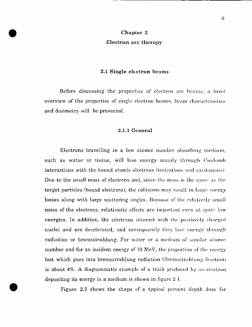
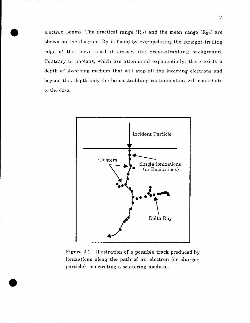
is about 4%. A diagrammatic example of a track produced by ail f!!C!ctroll
depositing its energy in a medium is shown in figure 2 1 .
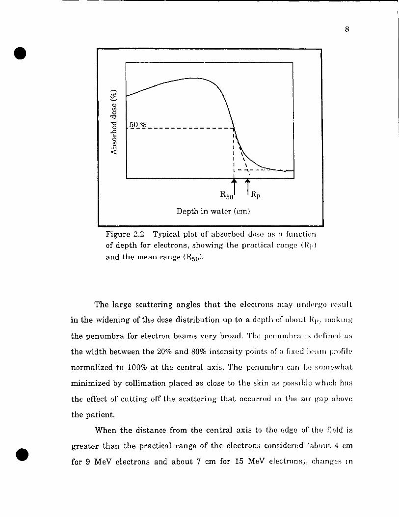
Figure 2.2 shows the shape of a typical percent depth dose for
•
7
clectron beams. 'l'he practical range (Rp) and the mean range (R50) are
shown on the diagram. Rp is round by extrapolating the straight trailing
('(J~e of the curvc until it crosses the bremsstrahlung background.
Cont.rary to photons, which are attenuated exponentially, there exists a
depth of abc.;orlnng medium that will stop a11 the incorning electrons and
bcyono th)" depth only the bremsstrahlung contamination will contribute
tn the dose.
Clusters
Incident Particle
~ Single Ionizations
(or Excitations)
• • ... ....-. ... \ Delta Ray
Figure 2.1 Illustration of a possible track produced by ionizations along the path of an electron (or charged
particle) penetrating a scattering medium .
•
Q) lfJ C
"0
] QQ~-------------.-e ~ 1
,..c::l 1 ~ 1
1 1 \ 1 - ""'\ - - - =-__ .-....-l
R50 Hp
Depth in watcr (cm)
Figure 2.2 Typical plot of absorbcd dose as a functillll
of depth fo:- electrons, showing the practical rall~c (l{I')
and the mean range (R50).
8
The large scattering angles that the electrons may undt>rgo rpsld t
in the widening of the dose distribution up ta a dcpth of about Rp , malullg
the penumbra for electron beams very broad. The penumhra IS ddif](·d as
the width between the 20% and 80% intensity points of a fixed br'am profile
normalized ta 100% at the central axis. The penumbra can be somcwhat
minimized by collimation placed as close ta the skin as pOSSI hic whlch has
the effect of cutting off the scattering that occurred in tl-je air gap above
the patient.
When the distance from the central axis to the edge of the fjeld is
greater than the practical range of the electrons considered (about 4 cm
for 9 MeV electrons and about 7 cm for 15 MeV electrons), changes ln
9
radiation field Slze will not change the central aXIS percent depth dose
bccausc electrons scattcrcd from the edges will not reach the central axis.
The efTect of the source-to-skin distance (SSD) on the depth dose
curve IS mostly se en within the build-up region. For ex ample, if the
distance t'rom the elcctron apphcator (cone) is increased then the percent
depth dose curve dccreases within the huild-up because of a decrease in
the arnount of scattcrcd clectrons. As the SSD is increased the beam
becorncs more hke a parallcl beam and this has the effect of decreasing the
dose wlthm the bmld-up rcglOn. Since the principal use of electron beams
is to treat from the surface to a certain depth with a dose as uniform as
possible, tht'n t.he surface dose must he as close to 100% as possible and a
typical distance bciwcPIl t.he electron cane and the patient's skin is 5 cm.
As can be expcctcd, tr.e main effect of changing the electrons'
incident. encrgy is to vary the dcpth of penetration or to change their
range. An IIlcrcase (decrease) in encrgy increases (decreases) the range.
'l'he combination of electron energy and bolus thickness can therefm e be
uaed to control the surface dose and the depth of treatment.
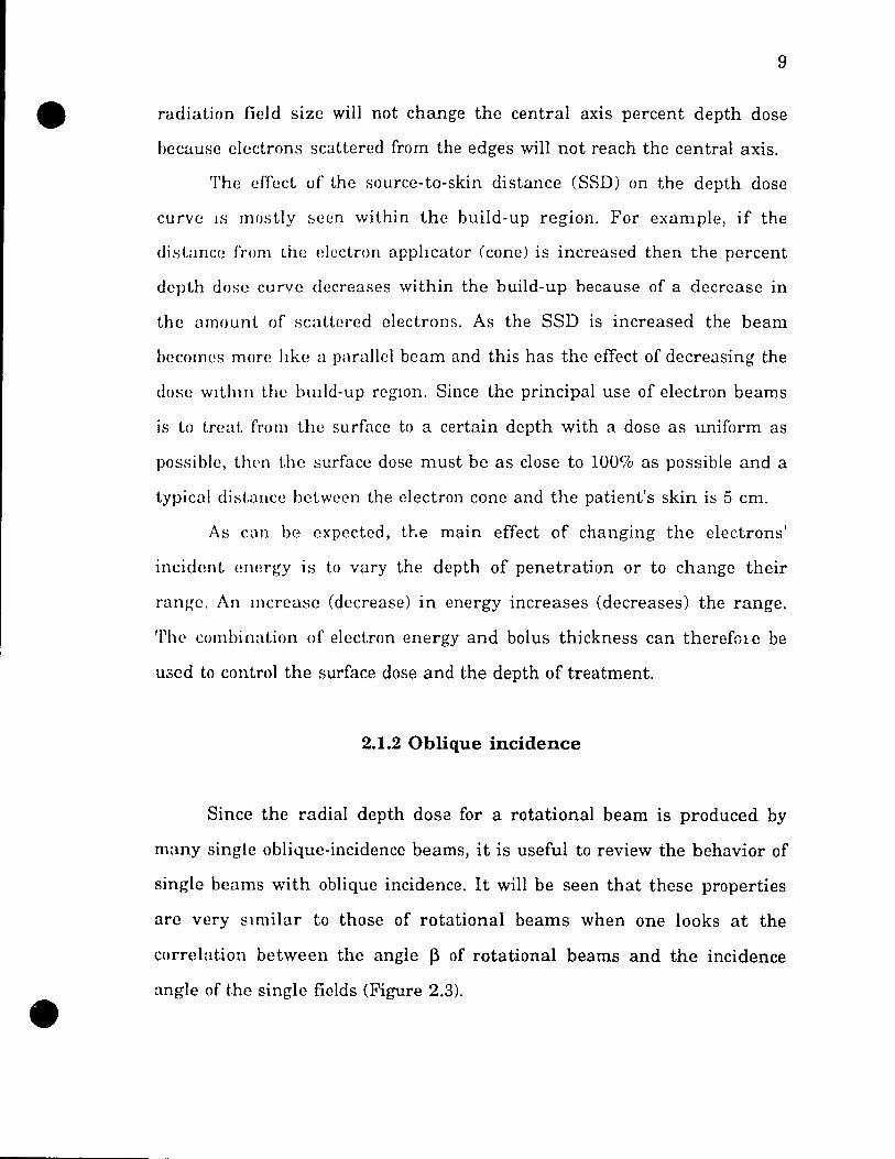
2.1.2 Oblique incidence
Since the radial depth dose for a rotational beam is produced by
many single oblique-incidence beams, it is useful to review the behavior of
single beams with oblique incidence. It will be seen that these properties
are very slmilar to those of rotational beams when one looks at the
correlation between the angle 13 of rotational beams and the incidence
angle of the single fields (Figure 2.3).
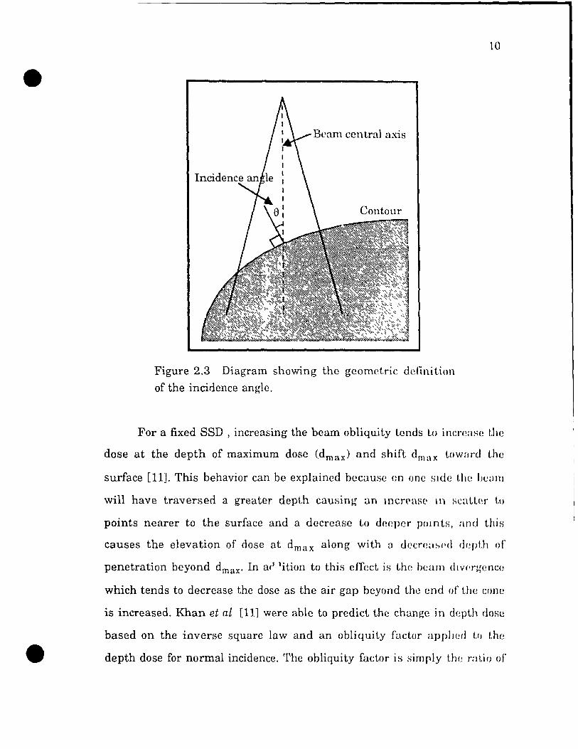
Beam central axis
Figure 2.3 Diagram showing the geornctric definition
of the incidence angle.
10
For a fixed SSD , increasing the beam obliquity lends lo incrcase the
dose at the depth of maximum dose (dmax ) and shift dmax towaru the
surface [11]. This behavior can be explaincd because en onc slde Uw heam
will have traversed a greater depth causing an mcrp(lse 111 scatter to
points nearer to the surface and a decrease to decper pOInts, and this
causes the elevation of dose at dmax along with a dt)cr(!a~('d dl!pth of
penetration beyond dmax. In ar lition tu this efTcct is the beam dlvl'rgence
which tends ta decrease the dose as the air gap bcyond the end of the cIme
is increased. Khan et al (11] were able to predict the change in depth dose
based on the inverse square law and an obliquity factor appJwù lo lhe
depth dose for normal incidence. The obliquity factor is simply ttH! ratio of

11
the iomzatlOn charges measured for the obliquely and norrnally incident
beums, with both measurernents performed at the same depth along the
central axis.
2.2 Physical properties of arc electron beams
This section will descnhe the effect of the beam collimation (which is
one of the paramcters setting this technique apart), the effect of the beam
paramelprs on the radIal pcrcentage depth doses, and how the ph0ton
co'1taminalIOIl affects the dose distnbution in electron arc therapy.
2.2.1 Beam collimation
The electron beams used for arc therapy are the same as those used
lI1 cOl1ventional stationary eiectroll beam therapy as far as the beam
broudening is concerned (i.e. scattering foils). The main difference lies in
the extensive collimatIOn required to obtain the desired dose distnbution.
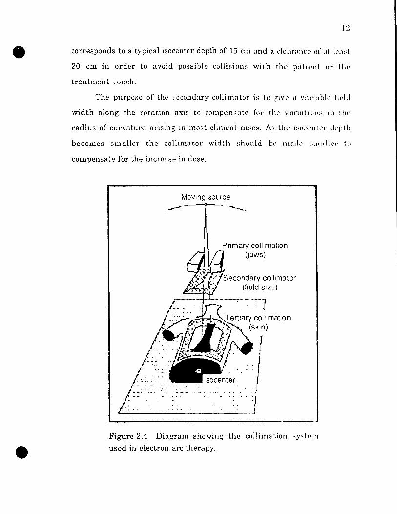
Figure 2.4 shows the three levels of collimation used in electron arc
therapy. The l'ledron applicators are not used with this technique because
the clearance between the end of the co ne and the patient is not sufficient
tu allow the gantry rotation.
The fi l'st rolli mation level is produced by the x-ray collimator which
al80 defil1l's the field wldth (light field at isocenter) used as a parameter in
the planning of a treatrnent when the secondary collimation is omitted.
When a secondary collimator is used the jaws are open sa that the primary
field is larger than the opening of the secondary collimator. The secondary
colli mator should be placed at least 35 cm from the isocenter which
•
12
corresponds to a typical isocenter depth of 15 cm and a clearance of aL 1l'<1!4t
20 cm in order to avoid possible collisions \Vith tl1l' patll'l1t. or t.lw
treatment couch.
The purpose of the 3econd:uy collimator lS tn gl\'l' a varIable lil'Id
width along the rotation axis to compensatc for the vanat LOn~ III tilt'
radius of curvature arising in most clinical cases. As tIlt' ISOCt'ntcr dept il
becomes smaller the colhmator width should hl' madl' smalll'r to
compensate for the increase in dose.
Movmg source
Pnmary collimation (pws)
Secondary collimator (field slze)
......... ~~~'-Tertlary colilméJ.tlon (skln)
Figure 2.4 Diagram showing the collimation sysU'm
used in electron arc therapy .
13
The increase ln dose when the isocenter depth decreases or when
the ssn increases is the opposite of fixed beams and this can be
undcrstood as follows. as the isocenter depth is decreased (SSD increased)
and t.he field size is kcpt constant, the angle of the arc that will contribute
t.o the dose at a givcn depth wIll increase. This geometrical effect is
stl'onger than the change in output due to the inverse square law. The
angle mcntioned above if-, closely re:lated to the angle ~ which will be
dcfined in detad ln t.he next chapter.
LeavItt et al l15] have used multIple arc segments \vith secondary
collimators tallored to each segment to take into account the change in
radius along the rotation axis as weIl as to compensate for the change in
radius withll1 the transverse planes. This compensation is necessary sinee
with continuous arc rotation the monitor units per degree are constant,
whereas for a pseudoarc technique the compensation within the
transverse plane CDn be donc by giving a different amount of monitor units
tü each bram. They also presented a method for determining the shape of
the secondary collimator which calcula tes the field width needed to keep
the dose at a dcsired depth along the rotation axis constant. The final
result is given by
l(w) x F(w) = DarcCr o,d,O,5) x 1 Darc(r,d,O,5) OAF(ylL) 2.1
where Hw) is the ratio of the dose at a point for an electron arc using
the secünddry light field width w tü the dose for the same arc for a
standard field width, which in the case of Leavitt et al. is 5 centimeters.
F(w) i8 slInilar to Hw) but for fixed electron fields. The product I(w) x F(w)

14
is obtained from a graph as a function of the field Slze w. This plot is
obtained from measurements performed with the saIlW geo Illl' 1 l'Y as 1:-; us('d
during a treatment. Darc(r,d.y.w) is the dose to a point al dt'plh li t'rom ail
electron arc about a patient (phnntom) of radius r at. a di~talH'l' y slIpl'l'iol'
or infenor to the central plane ul(}ng' thl' dlrt'ct ion ot' t lU' l'otal IOn :l'\. t:-; 01'
along the length of the field, re~mltmg from a S('c()I1(!ary collimator light
field width w at isocenter. OAF(vlL) is the otT-aXIS ratlO for ,\ fil'Id width spt
at the chosen standard (i.e. , 5 cm) and L is tlH' chst :InCl' t'rol1l t Ill' l'(\nt PI' of
the light field ta the edge of the light field along t111' rot al 1011 dXIS
Darc(rQ,d,O,5) .. . D (d ° 5) 1S the ratIO of th~ do~e from l'h,ctron arc 1Il t1w cl'nt.ral
arc r, , ,
plane at a depth d in a phantom (or patient) of raùius ro for a heam sd al,
the standard field width of 5 cm compared wlth the dos(' for a radius r.
This ratio as been shown by the authors tn be g"l ven by cquatlOn 2 2 lllldt'1'
the conditions that the effective source posItIOn remall1s fixpcl and t.h,,\' t.hl'
arc is large enough to completely include the beam prolilp lilr th(\ fixl'd
beam for the worst case, that IS for the smallest radius uspd c1inically
This result was originally presented by Khan et al. [121 and is gwen by,
Darc(r,d,O,5) =[ro-d] x [[~~O+~J Darc(ro,d,O,5) r-d f-r+d
where fis the effective source-to-Îsocenter distance.
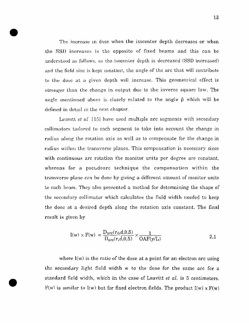
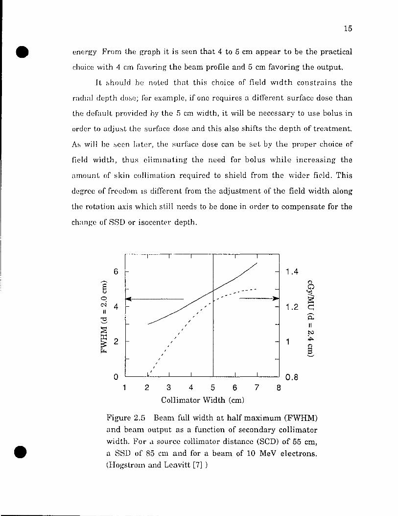
The choice of 5 cm for the standard sccondary collimator width IS
explained by Hogstrom and Leavitt [7] by looking lit the heam wldth and
dose output as a function of collimator width. FIgure 2 !j shows UJ(~ graph
they used in choosing the beam width. The data e()rrc~ponds 1,0 (] 10 MeV
beam, 85 cm SSD and a collimator placed at 45 cm f'rom the I~()center.
These curves depend strongly on the collimator position and on the
15
energy From the graph it is seen that 4 to 5 cm appear to be the practical
choice with 4 cm favoring the beam profile and 5 cm favoring the output.
It ~hl)uId he T10ted that this choice of field wldth constrains the
racüaI depth do~e; for exampIe, if one requin~s a ditTerent surface dose th an
the defauIt provided hy the 5 cm width, it will be necessary to use bolus in
order to adju!->t the surface dose and this also shifts the depth of treatment.
A~ will he ~een Iater, the surface dose can be set by the proper choice of
field width, thus eiimmating the need for bolus while increasing the
amount of skin collimation required to shield from the \vider field. This
degrce of frceù(lm IS difTcrent from the adjustment of the field width along
the rotation axis which still needs to be done in order to compensate for the
change of SSD or isocent(,f depth.
6 1.4 ,-.. n S Q u
~ 0 ~ 4 1.2 c::: Il ..-.,
"d 0-'-' Il ~ I.-.:l
~ 2 1 ~
n ~ !3
'-"
o 0.8 1 2 3 4 5 6 7 8
Collimator Width (cm)
Figure 2.5 Beam full width at half maximum (FWHM) and beam output as a function of secondary collimator
width. For d source collimator distance (SCD) of 55 cm,
a SSD of 85 cm and fOf a beam of 10 MeV electrons.
(Hogstrom and Leavitt [7] )
lG
The last level of collimation is the tertiary or skin collimation whlch
IS needed to shield outsidc the target volume and to minimi7.l' tlll'
penumbra ut the edge of the targe!. volume. As lIo(ed abovl.', tlll' :U'l':I to IH'
shielded de pends on the fidd size 1.l~('d d1.lring the !.rl'atJ11l'nt and Il e:ln tH'
found from the beam profile's measured 1Il au'. T1H' la~t two hl':lm~ al. !loth
ends of the treatment arc ~hou1d not contnbutl' tn the do~l' .Ju~t 1\1~\(h' tlH'
tertwry colhmator, or at least thclr contributIOn "hould lw 1ll'/~lIglhh'. 'l'hl'
skin collimation shou1d a180 be used to l'l'duce tilt' pl'l1u1l1hm ill t hl' plall(,
perpendicu1ar to the plane of rotation
2.2.2 Pseudo-arc technique
Boyer et al. [3J showed the feasibility of using fixed elecl.roll l)('al1l~
delivered in an isocentric manner to produce a conti IlUO\lS pledroll arc
dose distribution. Their technique did not use any secondary rollimator
and the field size was defined by the light field pr()duc(~d hy UH' x-ray
collimator with the lower jaws defining the lield width (narrow dllllensJOIl)
and the upper jaws definmg the field length. They round tha!' a ("OIlt.IIlIIOllS
dose distributIOn cou1d be obtmned wJth overiapplJ1g fiplds all/~rH·d III such
a way that the cross hair at the center of a gIVC'Il fic·ld would COI/H'lrle- wlt.h
the light field edge of the adjacent beam Shght van:1I,10I1!-> of ~II rl:I('(' dos(!
were observed for energies greater than 12 M"V but wilh IIU 1l01.ICC·:lbh·
variations at depths greater than dmax . Fmlure t,o cho()!->e t1H' proper
angular step would result in scallopmg of the dose distributIOn (undl'nJo!->e
between the beams).
For example, for an angular interval of 10" and an if-,ocenter depth of
15 cm, the mimmum field width necessary to meet this (~nterIa can h(:
17
calculatcd from simple geometry tü be about 6 cm. Ta facilitate the
tr!ChnHjUe such an interval can be used for ail treatments using a field
wldth greater thall about f) cm for a typlcal case of 15 cm lsoccntcr depth.
The 10" mterval 1<; used as a standard angular step at :'lcGill [21. 231
2.2.:J Effect of beam parameters on percentage depth doses
When a mcthod like the angle-~ concept [21115 used, the shape of the
PI)f) didates the energy and the field sizc which will produce the required
dcpth dose characten~tics \Vlth this methoJ. the surface dose can in sorne
caSl'S ({(Jr wide field widths or large p's) surpass that of fixed fields. The
l' ffc cV, the parameLers have on the radial depth do~e will be explained
assuming a treatIlH'nt technique which uses the secondary collimation
and a constant SAD (:-,ourcc-to-axis distance) machine. The parameters
that wIll be discussed are the SSD or isocenter depth, the field width at
isocentl'r definl'd hy the sl'condary collimator. the radius of curvature and
the elcdron lwam energy. There are more parameters that modify the
PD!) :-uch as the tyre of collimation (secondary and tertiary), the effective
50UrCl' posi tion. Ow fi ('Ici shape as defined by the secondary collimator and
variable numher of monItor units per beam for a non-continuous arc
tL'Chl11qUl': howevl'r, thesc other parameters are more or less fixed by the
tL'l'hniqu(' anJ Lan hl' assuI1lL'd tu hl' constant throughout the treatment.
It 15 diflll'u!t to separate the em~cts of the field size from those of the
SSD (or lsocenter depth) since an increase in SSD produces an increase in
the field sizl' with respect to a cylindrical phantom of constant radius. In
addition. therC' lH the obliquity ctTect as reported by Ruegsegger et al. [25]
which has an opposite elIect to that of the SSD and field size.
18
The individual effect of the SSD on the shapl' of tilt.' PD\) \S sllch
that a decrease of the SSD (increa:"l' \l1 i::-Ol'l'Iltl'l' dl'pth) d\:-.pl:ll'l'S dma \
toward largcr d('pths, lowers the ~tlrr:ll'l' dm;l' and ilH'l'L':I~{,S tlH' photon
contribution around the isoccntcr. ThIS dl'l'ct is dUt' to OH' rad th:!l a point
at a decper depth wll1 n>main in the bC:lm longpr than a pOInt clOSt'!" to tilt'
surface, The obliquity l'trect becoffics more important. as t hl' 1 :-'1H'1'llt l'r
depth is decreased,
An increase in field size produces efl'eets ~\milar tll ;l\1 1 1 IlTl':ISL' III
SSD which can be understood by the argument glvl'n abovl' that. thl'
change in field size compared to the ::aze of thL' phant,olll is tl1l' p;IrallH'tl'r
linking the SSD and the field wldth eCl'cds Also, thc obl\(!t11Iy l'I'I'I'cl
increases wi th increasing field size, 'l'he ('ITect of tilt.' hl':I111 l'1H'rgy 111
electron arc lS not very differcnt from its effpct l'or fixl't! fï"lds, t hl'I'(' <In'
small variations In the degrec to WhlCh tht' :-.urf':\t'(' do!-.p l'h:Ill~~t'S,
especially for low energies [25] for which lt f'eems that thr' ohltrplltv dTl'ct.
overrides the velocity e fTe ct, The velocity efTect IS thf' challgl' III t.ht, l.illH' a
point along a radii will be irradiated hy Hw r()t.alin~ bealll a:-. (\ f'ulld,101I of'
depth along the radii, If the secondary collimator IS omittt·d alld .JII:-'t. t.h(· x
ray collimator is used then the beam profile spread~ ou L d lW Lo the
increased scatter and the oblique pntry angle hecomes more llIlportallt 1 ~ l,
23] shifting d max toward the surface
The photon contamination accumulu tes at and around t lu' I!'>ocr!!l f.Pf
because of the rotational aspect of eledron arc therapy I~xprp~s('d as a
percentage of the electron dose at d mdx ' Lhe photon contributlOIl IIlcreases
with decreasing field size and SSD The close at the I~ocent.r·r cali "(~conu~
important, as much as 26 % for a boum energy of IH MeV, ,Ill ISO('Pfltef
depth of 15 cm, an electron arc of 1800 and a secondary collimator wldt.h of
---- --------------
19
!) cm fI5]. This dose is very much dependent on the machine (scattering
foils) and should be measured for ail treatment geometries used clinically.
Pla et (Ll. [221 have Jnvestigated the photon contribution for a pseudoarc
technique wlth angular mtervals of 10° and primary collimation only.
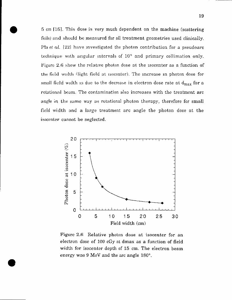
Figure 2.6 ~how the relative photon dose at the lsocenter as a function of
the field wllhh rJight field at lsocenter). The lncrease In photon dose for
small field vndth IS duc to the decrea~e in electron dose rate at dmax for a
rotational beam. The contamination also increases with the treatment arc
angle in the same way as rotational photon therapy, therefore for small
field width and a large treatment arc angle the photon dose at the
isocenter cannot be neglected.
20 -,--r-r--r-r-
'""'" ~\J (.,,, "-'
s.. ~ 1 5 ...., ~ (]) (.)
0 if.! ..... ...., 1 0 ~
~ if.! 0
"'t:l
~ 5 0 ... 0
...c: p..
o 1 1 1 1 1 1 t 1 1 1 1 1
o 5 1 0 1 5 20 25 30 Field width (cm)
Figure 2.6 Relative photon dose at isocenter for an
electron dose of 100 cGy at dmax as a function of field
width for isocenter depth of 15 cm. The electron beam
energy was 9 MeV and the arc angle 180°.
20
2.3 Pencil beams in electron arc thcrapy
The genenc pencil beam algorIthm (Hog~trolll ct al. I~)j) fOl" IiXl'd
electron beam will be presented first and sub~wqul'ntly tllL' l'~t l'l1Siol1 tu
the algorithm for electron arc therapy will be presl'nted (Hog~tl'(}ll\ t'f al.
[6]).
The purpose of the pencil beam algorithm IS to provldp a model l'or
the calculation of electron beam dose distrIbutions lIlclud1l1g t Ill' jll'l'S('lll'l'
of inhomogeneous tissue by making use uf CT data 'l'Iw pnm'lpll' or addll1g
pencil bearn distnbutions to obtam the distnbutlon of a \\'H!l' field \Vas first
demonstrated by Lillicrap et al. [16] (975) by companng t IH' ~\Il11ll\ati()n
of measured pencil beams with the mcasured di!->tnhut Ion of a hro;u! IH'arll
The pencil beams were measlifcd in a homogcneou:-, phantolll hut li
mathematical model is needed to predlct th0 dlstrihutlOn of thl' pencil
beams in inhomogeneous media since such IT1C(lSUremellts would 1)(,
impractical.
A brief summary of the input data and the calculatloll stl'pS
involved in the model will precede the mathematical description of the
algorithm. There are two regions that are considercd 111 the algoflthm; UH'
air gap and the medium (or patient). The successive behavior of' LIli' fH'llcil
beams i5 treated as follows: the pencil heam~ start aL th,· boLLolll ('dg-e of'
the secondary collimator (electron apphcators or cones), spread III t1w (Ill'
according to measured data, penctrate the medium, and thcn spread
according to a mathematical model callcd Ferml-Eyges tJwory ba!-.pd on
multiple Coulomb scattering compounded tn the same spreadmg as in air.
The pencil beam has a profile that can be described In aIr and III medium
by a Gaussian; the Gaussian in the medium is in fact the convolution of
21
t.he in-air spreading with in-medium spreading. The dose at a point in the
medIUm IS the s um of all the penci1 beam doses at that point. The
spreadlllg of the pencil beams in aIr is obtained from a set of broad beam
profiles at various source-to-chamber disLd.:1C'pc;; the position of the virtua1
~ource can also be extrapolated from these rneasurements and used
subsequenUy lo take into account the beam divergence. The Fermi-Eyges
theory howéver does not include the 10ss of electrons as the beam
penetrates the medium and a correction must be app1ied to take into
account this depth effect. The PDD for the field considered is used to force
the result of the surnmation of penci1 beams to exactly reproduce the
measured PDD. This gives a correction function used thereafter in the
model that accounts for the electr(ln 10ss. The inhomogeneities are
i ncl uded 1Il the model by the use of CT numbers which directly gi ve the
linear stopping power from a rneasured calibration curve. An effective
depth is round along the line formed by the source point and the
calculation pomt that modifies the PDD correction and the electron energy
nt depth. The Fermi-Eyges theory also uses this data in finding the
standard dcviation of the Gaussian due to multiple Coulomb scattering.
2.3.1 Angular spread in air and virtual source position
The data used to de termine angular spread in air and virtual source
posi tion arc the beam profiles in air measured at various source- chamber
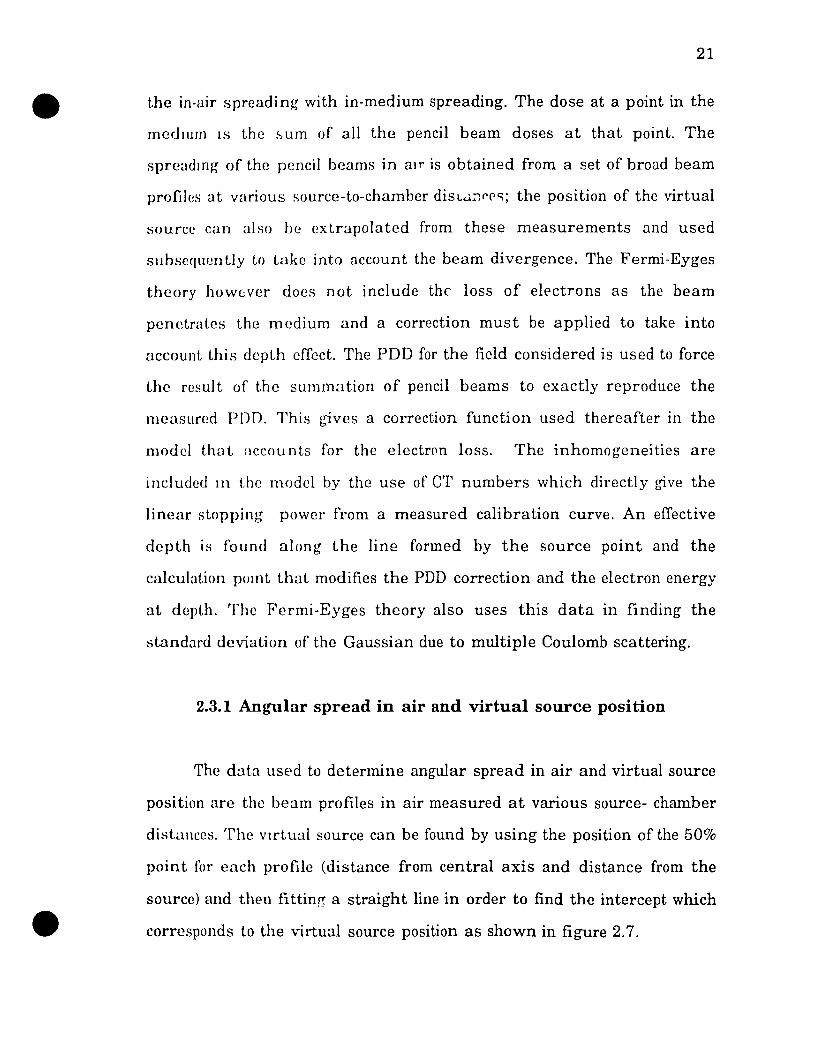
distances. The vlrtual source can be found by using the position of the 50%
point for each profile (distance from central axis and distance from the
source) and then fittinrr a straight Hne in order to find the intercept which
corresponds to the virtual source position as shown in figure 2.7.
1 0 ~
l'''--'--'-~'--· r-·- ,-
/
8 ,.
,-., • ~ S .-~ u ct!'-'
~~ 6 · ... 0 "t:l1O
rJ.l Il
.~~ 4 Isocenter ~O SAD = 84 cm 0"" ~
2
0 1 1 L-L_L __ L_l . L -' _
0 20 40 60 80 100
Source-chamber distance (cm)
Figure 2.7 Graph showing the intercept determining
the virtual source posit.ion for a 9 Mc V electrol1 heam
and a bearn width of 15 cm. The isocenter is 1(:i cm l'rom
the machine isocenter.
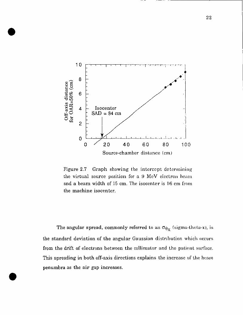
The angular spread, commonly referred to as (j8x (sigma-thcla-x), is
the standard deviation of the angular Gaussian distnbution which occurs
from the drift of electrons between the collimator and the patient surface.
This spreading in both off-axis directions explains the increase of Hw beam
penumbra as the air gap increases.
cre x
Penumbra
Figure 2 8 Diagram showing the geometric relation
between the penumbra width and the standard
deviation of the profile. Also shown is a Gaussian profile
with the standard deviation.
23
e
<Js x cau be calculated usmg the moments of the linear angular
scattering power as shown in Hogstrom et al. [9] but it is simpler to use the
slope of the plot of in-air penumbra width as a function of source-detector
distance. Figure 2.8 graphically shows how <JSx is related to the penumbra
width and the :-:;ource-to-detector distance, the tangent of the angle ($) is
proportional tü the slope of the line obtained by plotting the penumbra
width as a function of source-to-detector distance. The penumbra width
cau be defined either as the 90%-10% or 80%-20% width, and O'Sx can be
calculated using equation 2.3 .
•
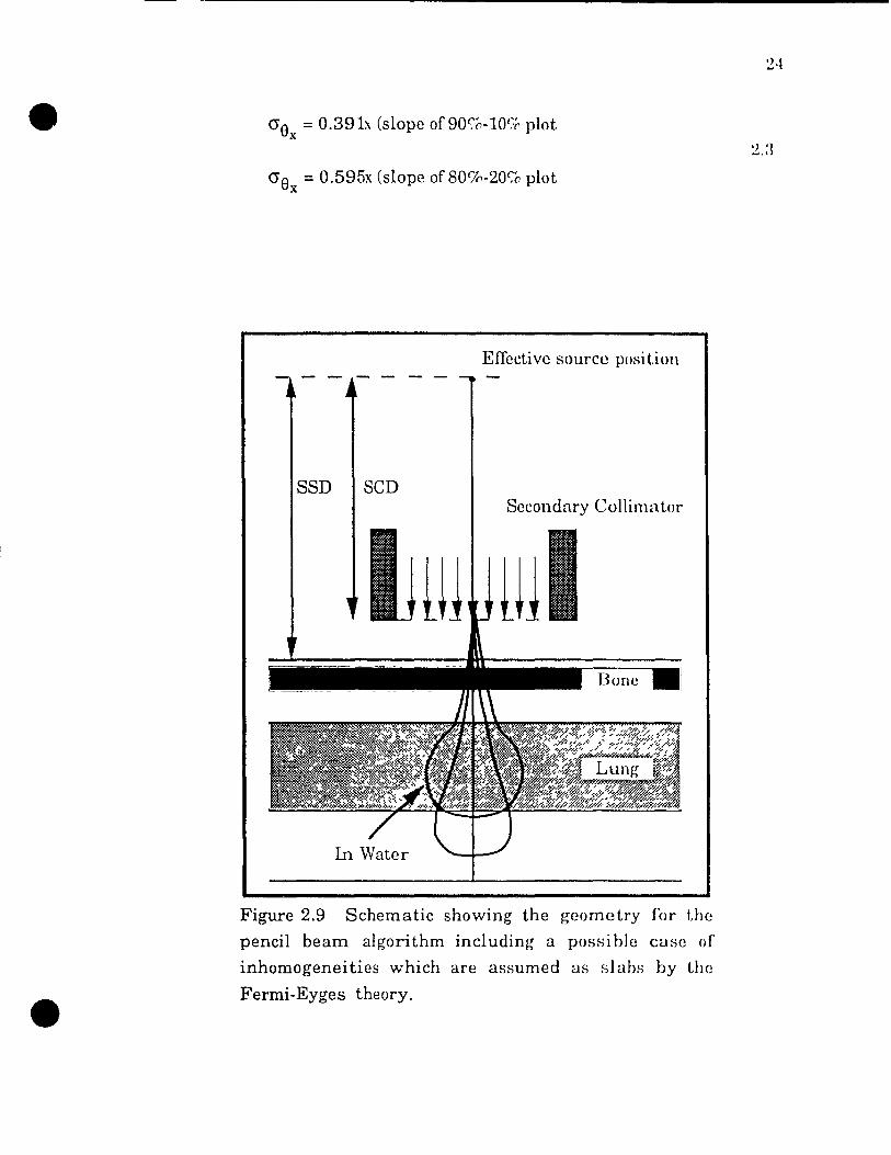
(Je = 0.391:\ (slope of 90<7'(,-10(;0 plot x
(Jex
= 0.595x (slope of 80%-20% plot
Effective source posi Lion
SSD SCD Secondary Collimator
Ul Ul
Figure 2.9 Schematic showing the geometry for the
pencil beam algorithm including a possible case of
inhomogeneities which are assumed as slabs by the
Fermi-Eyges theory.
25
2.3.2 Fermi-Eyges theory (Spreading in medium)
Eygcs modified the EmaIl-angle multiple scattering theory first
dcveloped by Fermi ta incl ude inhomogeneities with slab geometry
constraint and energy 1055, ta obtam what is known as the Fermi-Eyges
theory. The thcory eonsiders the inhomogeneities underlying the central
aXIs as slahs extending infinitely laterally and this is an approxImation
wlllch breaks down whcn mhomogcneous structures present sharp edges
paralI('1 Lo the beam (Flgure 2.9). Although the theory treats the energy
1088, it ducs not mc1ude the faet that eleetrons which are lost have their
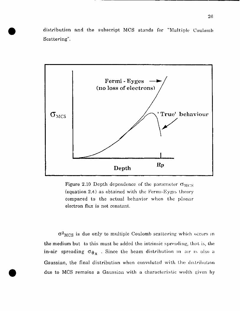
cnergy completely absorbcd, resulting in a behavior illustrated in figure
2.10.
'l'he basic Fermi-Eyges model gives the probability f (X,Y,Z) to find
an clectron at a depth Z with coordinates between X and X+dX, y and
Y+dY for an eleetron incident in the Z direction at (X=O, Y=O, Z=O) as
where 2.4
cr~CS = ~ LZ
(Z-u)2 T(u) du
and '1'( u) is the lincar scattering power of the medium, defined as the
incrcase of the menn square angle of deflectian per unit of path length at
dcpth u [T(U) ~ de:~u~ l cr2MCS is a measure of the width of the Gaussian
2(1
distribution and the subscript MeS stands for "l\lultipll' Coulomb
Scattering" .
Fermi - Eyges (no 10ss of electrons)
(j'Mes 1 True' behavioul'
\/
Depth Rp
Figure 2.10 Depth dependence of the paramet.er ()MCS
(equation 2.4) as obtained with the Ferml-Eygl'~ thcory
eompared ta the aetual behavior wh en the plallar
electron flux is not constant.
cr2MCS is due only ta multiple Coulomb scaltering which (Jcclirs III
the medium but to this must be added the intrinsic sprpadillg, lhal i~, th(~
in-air spreading <J8 x . Sinee the beam distrihution 111 ,lIr I~ also a
Gaussian, the final distribution whcn convolutcd with t.he dl~trihl1tlOn
due to MeS remains a Gaussian with a charadcrislic wlflth given hy
27
(J2 rtJed = (j2 MCS + 0'8 x2 . This is the sigma which must be J.sed when
calculaling the dose in the medium.
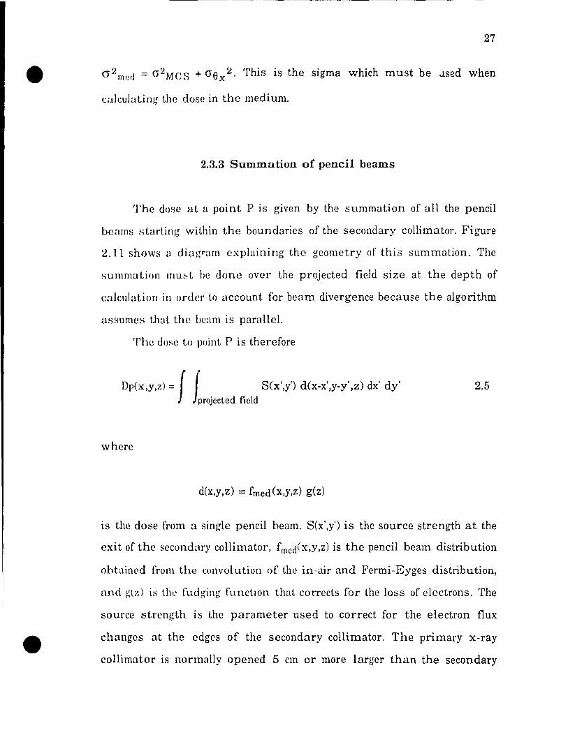
2.3.3 Summa tion of pencil beams
The dose at a point P is given by the summation of aIl the pencil
beams starting within the boundaries of the secondary collimator. Figure
~.11 shows a diagram explaining the geometry of this summation. The
summation mu~t be done over the projected field size at the depth of
calculation in orcier to account for beam divergence because the algorithm
assumes that the ueam is para Il el.
'l'he dose to point P is therefore
Dp(x,y,z) = f f S(x',y') dex-x',y-y',z) dx' dy' projccted field
2.5
where
d(x,y,z) = fmed (x,y,z) g(z)
is the dose from a single pencil beam. S(x',y') is the source strength at the
exit of the secondary collirnator, fmed(x,y,z) is the pencil beam distribution
ohtained l'rom the convolution of the in-air and Fermi-Eyges distribution,
and g(z) is the fudging functlOIl that corrects for the 10ss of electrons. The
source strength is the parameter used to correct for the electron flux
changes at the edges of the secondary collimator. The primary x-ray
collimator is normally opened 5 cm or more larger than the secondary
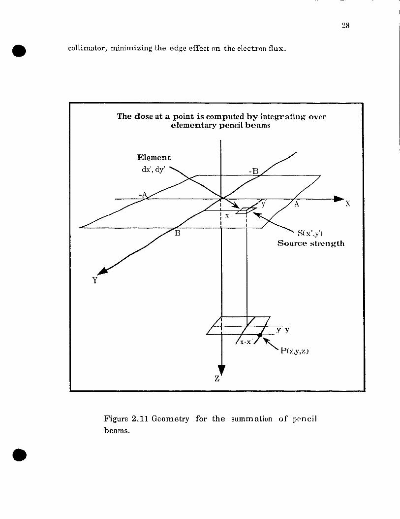
28
collimator, minimizing the edge effect on the electron flux.
y
The dose at a point is computed by Întegrating over elementary pencil beams
Element clx', dy'
'---'r---"l'---1IIt--
S(x',y')
Source strength
y-y'
'P(X,y,Z)
z
Figure 2.11 Geometry for the summation of ppncil
beams.
x
29
2.3.4 Correction for 10ss of electrons
As previously statcd, the Fermi-Eyges theory does not eompletely
reproduce electron transport sinee it does not consider the 108s of electrons
when the cnergy is completely absorbed. To correct for this, the
summation shown at equatlOn 2.5 is forced ta be equal tü the measured
central axis depth dose:
Dmeasurpd(O,O,Z) =f ( dC-x',-y',z) dx' dy' lprojeeted field
2.6
where S(x' ,y') was taken to be equa1 to 1 for simplicity. From this equation
and [rom the definition of the dose due to penci1 beams, as defined in
equation 2 5, the function g(z) can be isolated and is given by,
2 1 [A( 11 Z)] [B (lI Z )] ) g(z) = [SSJ2+z] Dmeas(O,O,z) \erf SSD erf SSD
SSD fi O'med(Z) fi O'med(Z)
2.7
where the error function is defined as
erf(x) = ~ (X e-t2dt. Yi lo
2.3.5 Use of CT numbers
The CT numbers are used tü calculate an effective depth zeff using
the lin car stopping powers übtained from a calibration plot of Seo] as a
functiün of CT number. The linear stopping power Seo] = dE is the amount d.x
of encrgy lost pcr unit length by a charged particle in producing ionization
ao
in the ab80rbing medium. Assuming that the Imeur ~toppin~ power IH
relatively independent of electron energy twhich is justitil'd whl'Il
considering water and normal body tissues), the l'n'l'dive dt'pth l~ round
with the following expression :
where Lü is the distance betwcen the- secondary collimalo!' and t1H' patil'nt.
skin. The origin is taken at the skin anu the-ref'ore the mt.eg-ration is dOlll'
from the secondary collimator to a depth z.
The function gmed(z) can be found fronl the efTl'ctiVl' dppth hy using-
g(z) for water or the function g(z) founu using the IllL'<lSUrL'd dept Il dOSl' i Il
water. The correspondence between the medium and wa(,l'l' i s dOlll'
through Zeff ;
2.9
In the calculation of O'med (from the Fernu-Eygcs result) the linear
scattering power T(u) is needed and it can be round through the llIean
energy Ez approximated by,
~. 1 ()
where EO 18 the average energy at the surface and should be calculated
from the relation Eo = 1.919 Rp (cm) + 0.772 . A table of val UC!S for
T water(E) is used to find T med(E) from the ratio T med(l~)rl'wat(!r(E) w hlch is
a8sumed ta be independent of ~.
31
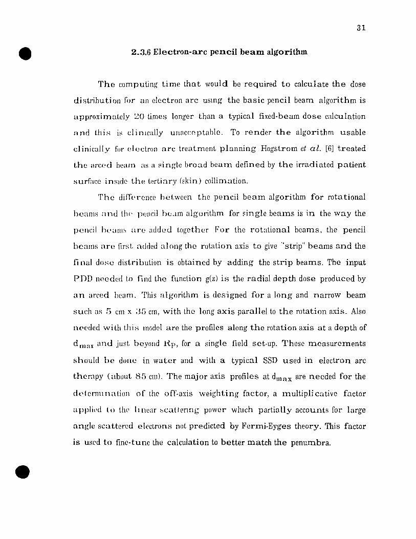
2.3.6 Electron-arc pencil beam algorithm
The computing time tha t would be required ta calculate the dose
distrihution for an clectron arc usmg the basic pencil beam algorithm is
approxirnutely ~() times longer than a typical fixed-beam dose calculation
and this is clinlcally unacceptahle. '1'0 render the algorithm usable
cl inically f(Jr electron arc treutrnent planning Hogstrom et al. [6] treated
the arced beam as a single broad bearn defined by the irradiated patient
surface insHlc the terti3ry (skin) collim.ation.
The difTprence hetween the pencil beam algorithm for rotational
beams and Uw pencil bl:.lm algorithm for ~ingle bearns is in the way the
pencil healll:-' are added together Por the rotational beams. the pendl
bcams are first added along the rotation axis ta give ·'strip" beams and the
fi na) dose distribution is obtained by adding the strip bearns. The input
PD1) nceded 1,0 find the function g(z) is the radial depth dose produced by
an art'cd bcam. This algorithm is designed for a long and narrow beam
such as G cm x ~H) cm, with the long axis parallel to the rotation axis. Also
n('cded with this model are the profiles along the rotation axis at a depth of
d max and jllst. heyond Hp, for a single field set·up. These measurernents
shollld be done in water and with a typical SSD used in electron arc
therapy (about 85 cm). The major axis profiles at dmax are needed for the
dl.~tcrnl1nati()n of the off-axis weighting factor, a rnultipU cative factor
appliL'd to Ll1l' hnear ~cat.tenng power WhlCh partially accounts for large
angle scattered electrons not predicted by Fermi-Eyges theory. This factor
is uSl'd ta fine-tune the calculation to better match the penumbra.
As a wholc, this modified algorithrn for the dOSt' calculation of
rotational beaIns is the same as that for fixcd bl'am~. both llsing tlw Fl'rmi
Eyges theory as the foundation for n"lultiple scattl'I'ing- within the l11l'dlllll1
and using CT numbers in the same manner.
33
Chapter 3
The angle p concept in electron arc therapy
3.1 Physical aspect
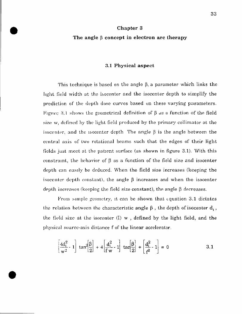
This technique is based on the angle p, a parameter which links the
IIght field wielth at the Ï:-,ocenter and the isocenter depth to simplify the
prediction of the elepth dose cun'es based un these varying parameters.
Il'lI;Ht'ë :1.1 shows t.he geornetrical definition of p dS a function of the field
size w, dcfined hy the light field produced by the primary collimator at the
isocentt'r, and the l::,ocenter depth The angle p i8 the angle between the
œn tral axis of two rotational beams such that the edges of their light
fields just meet at the patIent surface (as shown in figure 3.1). \Vith this
constramt, the hehavior of ~ as a function of the field size and isocenter
depth ean eusdy be deduccd. When the field size increases (keeping the
isocenter depth cOIlslant), the angle ~ increases and when the isocenter
depth increases (keeping the field size constant), the angle ~ decreases.
From ::-'lmple geometry, lt can be shown that lquation 3.1 dictates
t.he relation between the characteristic angle ~ , the depth of isocenter dl ,
the fil'ld size at the isocenter (l) w , defined by the light field, and the
physical source-axis distance f of the linear accelerator.
3.1
f
d· 1
\1 ~ -------
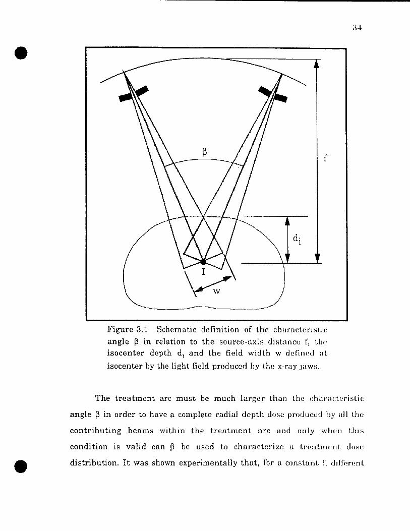
Figure 3.1 Schematic definition of the chaructenstlc
angle ~ in relation to the source-ax:s distance r, Uw isocenter depth d) and the field width w defined at
isocenter by the light field produced by the x-ray Jaws.
The treatment arc must be much larger than the ehanlcte"ist,ic:
angle ~ in arder to have a complete radial depth dose produced by ail the
contributing beams within the treatment arc and only wlH'1I thls
condition is valid can ~ be used tü characterize a tf(~atnwnL dose
distribution. It was shown experimentally that, for a constant f, ddfrmmt
35
combinations of w and d) giving the same ~, produce very similar radial
percentage dcpth doses [22, 23].
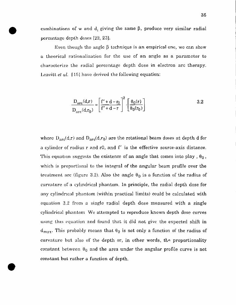
Even though the angle ~ technique is an empirieal one, we ean show
a theorical rationalization for the use of an angle as a parameter to
eharadcrize the radial percentage depth dose in electron arc therapy.
Lcavi tt el al. [15 J have dcrivcd the following equation:
Dnrc(d,r) = [f' + d _ro]2.[ 80(r)] D (dr) f'+d-r SO(rO)
arc ' 0
3.2
whcre Darc{d,r) and DarcCd,ro) are the rotational beam doses at depth d for
a cylindcr of radius rand rO, and f' is the effective source-axis distance.
This cquatlOn suggcsts the existence of an angle that cornes into play, 80 ,
which is proportional to the integral of the angular beam profile over the
treatmcnt arc (figure 3.2). Also the angle So is a function of the radius of
curvature of a cylmdrical phantom. In principle, the radial depth dose for
any cylindncal phantom (within practical limits) could be calculated with
cquation :3.2 from a single radial depth dose measured with a single
cylindrical phantom Wc attcmpted to reproduce known depth dose curves
usmg t.hlS l'quation and found that it did not give the expected shift in
d max . This probably means that 80 is not only a function of the radius of
curvature but also of the depth or, in other words, tl./O! proportionality
constant bctwcen 80 and the area under the angular profile curve is not
constant but rather a function of depth.
•
3G
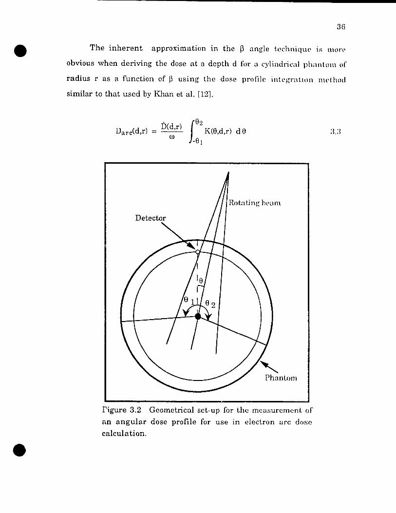
The inherent approximation in the ~ angle techniqlH\ is more
obvious wh en deriving the dose at a depth d for a cylindrical phantom of
radius r as a function of ~ using the dose profile intl'g-ratlOll Ilwt.hod
similar to that used by Khan et al. [12].
DarcCd,r) = Ded,r) û.) f
82 K(8,d,r) cl e
-81
Phantom
Pigure 3.2 Geometrical set-up for the rneasurcrnent of
an angular dose profile for use in electron arc dose
calculation .
37
The dose for an electron arc at a point in the phantom DarcCd,r) ean
be caleulated us mg equation 3.3, where KC8,d,r) is the angular dose profile
at a depth d for a cyhndncal phantom of radius r, DCd,r) is the dose rate for
a fixed field at a depth d and SSD = (f-r), (ù is the speed of rotation
(radians/min) and 8 1 , 8~ are the angle limits of the scan rneasured from
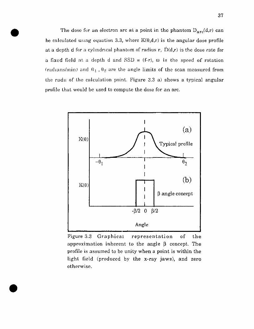
the radll of the calculatiün point. Figure 3.3 a) shows a typical angular
profile that would be used tü compute the dose for an arc.
(a) K(8)
K(8) (b)
13 angle concept
-pJ2 0 pJ2
Angle
Figure 3.3 Graphical representation of the
approximation inherent to the angle Il concept. The
profile is assumed to be unit y when a point is within the
light field (produced by the x-ray jaws), and zero
ütherwise.
38
The second plot (figure 3.3 (b)) graphically shows the approxlll1ation
that must be made in order to derive equation 3.4 WlllCh g-iws OH' dOSl' at. a
depth d for a phantom of radius r, glVen a reference dose also at dppt h d
but for a radius ro and the two respective (Ys. 'l'lus apprOXlIllat IOn IS b"t iL'r
justified when considering the rntio of two dOSl'S as tt IS dOlH' III t Ill'
development of equatiol~ 3.4 sinee the integral in equatio\1 :~:~ is
proportlOnal to ~ (or sorne other angle), as discussed parhe .. wtt h t1H' l'l'suit.
of Leavitt et al. [15].
2 1 f' + cl - ro 1 ~(r) DarcCd,r) = DarcCd,ro)lf'+d_r '~(ro)
:~. ·1
The effect of the field size was dlsregarded in the denvat ion of t.hlS
equation, which is a reasonable assumption for sizes g-reat.er t.han tIlt'
practical range of the electrons. The rotation speed was also cOJlsidl'red
constant.
The ~ technique uses measured radial dcpth dOHc eurves, l'ach
associated to a characteristic angle ~, 1,0 compute the dose dist.ribuUon. A
set of radial PDD as a function of ~ i8 the basic data froIn which tlw isodoHl'
distribution can be calculated. EquatIOn ;~ 4 for d=() IS lI~('d t,o lilld t111'
relative dose along the surface (patient skin) wi th resp('ct 1,0 the dose ai li
reference point. The ~ technique can be used 1,0 force the surfacl.' dose ai
the beam entry points to be as uniform as pOSSIble by varylllg t hl' beam
weights within the same arc (pseudo-arc In the case of the MC<;dl r~
technique). The number of monitor units for ca ch bcam is proporttonal lo
the inverse of the surface dose, that is, if the surface dose deer('a:,(~s t.hen
the number of monitor units for that bcam must increase to cornpensate.
39
The calculation of the monitor units for a given arc assuming that
the nurnber of monitor units for the reference point is known, is do ne as
l'ollows:
')
MU: = MU . [ f' - d) ]~. ~ref J ref f' -d CL
ref !-Il
3.5
where MU) and MUref are the number of monitor units fûT the ith beam
and the rel'erence beam respectively, d) and dref are the depth of the
isocenLer ulong the central aXIS of the ith and reference beams, ~i and ~ref
are the characteristic ~'s carresponding to thelr respective isocenter
dppths and fi i~ the effective source-axis di ",tance The actual surface dose
obtained \Vith the mOI1ltor UI1lts calculated with equation 3.5 will not be
absolutely uniform since tü obtuin a desired surface dose a11 of the beams
should have the ~ame weights (monitor units). As WIll be shawn in the
second part \Jf this chapter, the surface dose for a pseudo-arc treatment
wIth unequal monitor umts per beam can be calculated by a weighted
beam profile correction and the radial PDD can be scaled with the
caIculuted surface dose to reflect the same surface dose, giving therefore
the depth dose dIstrIbutlOn for that particular beam entry point.
In practice, the way this technique is used is as follows: i) the choice
of the surface dose and depth of maximum dose is made, and a PDD curve
is chosen from the baSIC PDD set, il) from the selected PDL we obtain the
characteristIc ~ at the reference entry point and the beam energy
required, iii) from ~ref and the patient contour which defines the isocenter
dl'pth at the rl'ference drer, the field width w can be calculated, iv) with w
constant for the treatment arc and with aIl of the isocenter depths at the .
---- ----- ",- .. -
e.
40
entry points (di) the dose distributIOn and the amount of monitor umt.s per
beam can be determined. 'This method differs from the tixt.'d narrow lwam
technique in that the depth dose curve 18 ehosPI1 to suit tlH' phy~H'lall's
choice and ehminates the construction of bolus tn adJl1st t h~, :-.urfacl' dosl'.
Bolus is still used to replace missing tissue and to oITst't, tilt' dO~t' in critical
regions such as the lung in the treatment of the dll'st, wall
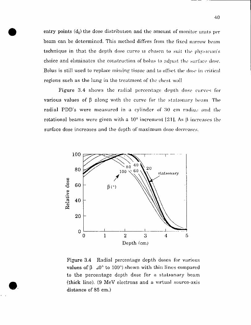
Figure 3.4 shows the radial percentage dppth do~-H' rurvl''' l'or
various values of ~ along wIth the curve for the statlOnary Ill'am TIH'
radial PDD's were measured in a cylinder of :30 cm radiu.; and tl1l'
rotational beams were given with a 10° incremrnt (21]. As p incI'l':uws t.IH'
surface dose increases and the dcpth of maximum dose clecrl'ë:\ses.
100
80
Cl.) (lJ
0 60 "'d Cl.)
> ..... ..., Cj 40 ....... Cl.)
~
20
0 0
Depth (cm)
Figure 3.4 Radial perccniage depth doses for various
values of ~ ~Oo to 100°) shown with thin lines compl.lred
to the percentage depth dose for a statlOnary beam
(thick line). (9 MeV elcctrons and a vlrtual source-axis
distance of 85 cm.)
41
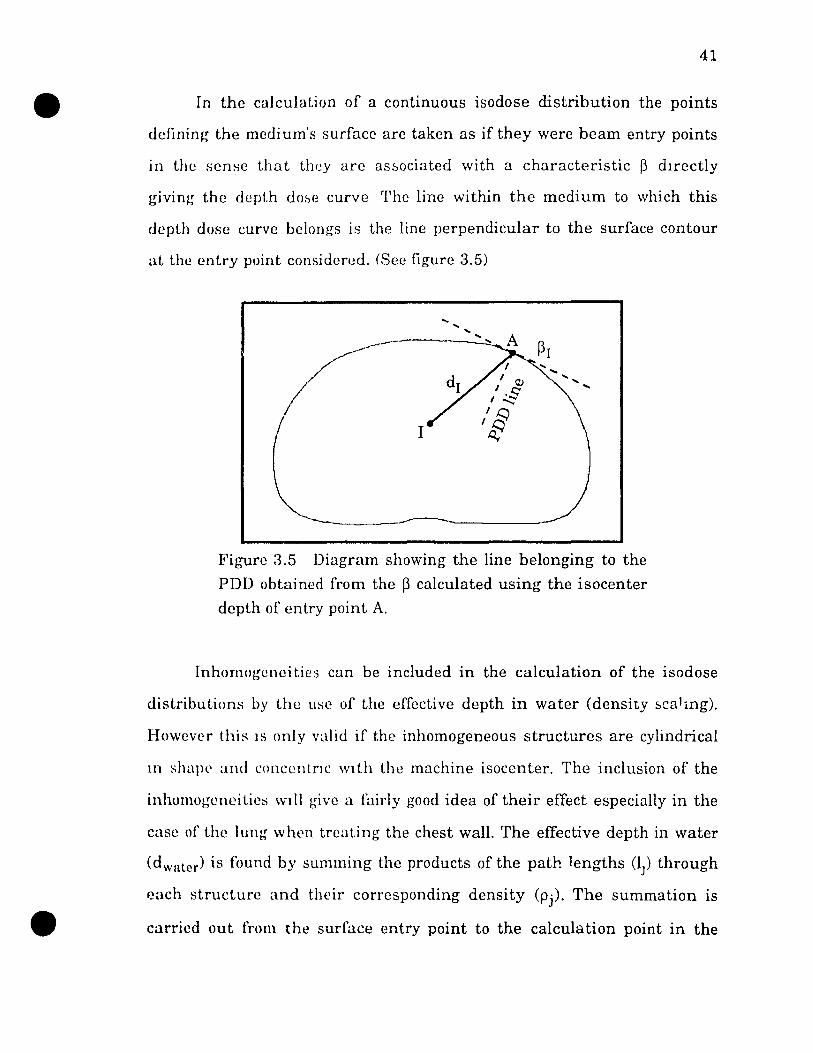
In the calculation of a continuous isodose distribution the points
dcfining the medi um's surface are taken as if they were beam entry points
in the sense that they arc as~ociated with a characteristic ~ dlrectly
giving the dcpth dose curve The line within the medium to which this
depth dose curve bclongs is the line perpendicular to the surface contour
al the entry point considered. (See figure 3.5)
... .... .... .... ...
l
.... "
Figure 3.5 Diagram showing the line belonging to the
PDD obtained from the ~ calculated using the isocenter
depth of entry point A.
Inhomogencities can be included in the calculation of the isodose
distributions by the use of the effective depth in water (density t,ca1lng).
Howevcr this IS only valid if the inhomogeneous structures are cylindrical
1Il shapt' and concentnc wIth the machine isocenter. The inclusion of the
inhomogeneilies will givc a fairly good idea of their effect especially in the
case of the 1 ung w hen trcating the chest wall. The effective depth in water
(dwater) i8 round by summing the products of the path lengths (lJ) through
cach structure and their corresponding density (Pj)' The summation is
carried out l'rom the surface entry point to the calculation point in the
42
medium as given ln equation 3.6, where n IS the Humber of segments
between the surface to the calculution point.
n
dwater = l Ij' PJ J = 1
Pla et al. [22] investigated the electron dose rate nt. tlm.n: for tilt'
pseudo-arc technique used at McGill. Hcrc the dose ratl' at a gwen point in
t.he phantom is defined as the ratio of the given L'!t>ct.rol1 dosp t 0 till'
number of monitor units per st:ltionary eledron Iwam. It wa~ f'ound
experimentally that only the calibration for one combinat 10 Il of fi(,ld SIZl'
and ',socenter depth per electron energy is necded tn calculate thl' t'I('l't,rllil
dose rate for any other combination. For a constant 13, thl' i nv('rs(' squan'
law relationship using the effective source position Lan be lIsed to
calculate the dose rate for a different isocentcr depth as ShOWll in equat.Îoll
3.7 [Figure 3.6J:
This relationship makes sense because a constant 13 rncans thut the
measurement point will remain in the beam for the sume arnouilt of Urne
and, for electron beams, the field size effect is small for fi(~ld :-'lzes gl'patcr
than practical range which IS the case for the r~ pscudo-arc lcdllllqUC
Since in this case ~ is constant, the field size w{f3) can be calculatr!d with
the known ~ and the desired dI(B) with the use of equation :3.1.
43
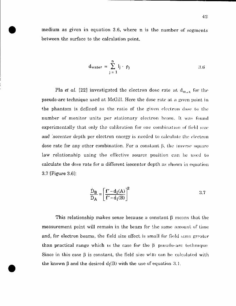
The clectron dose rate for a rotational beam increases linearly with
the field width and a similar observation was made by Leavitt et al. [13, 14J
in their study of multilcaf collimators in electron arc therapy. The photon
contamination at the isocenter, as discussed in section 2.2.3 and shown in
fi~ure 2.fj, is inversely proportional to the electron dose rate at the nepth of
maximum dose for rotational beams, the higher the electron dose rate the
)owcr the photon contributIOn at isocenter since the photon contamination
does not change Wl th field size.
/ /
/ /
/
/
Points A and B have same p
/
Linear /,//
.!.ele/ationSh~~~ / 1
/
/ 1
/ /
/ -/-
/ /
/
w (B)
Field width
/
// dI(B)
w (A)
Figure 3.6 The combinations (w(A), dI(A» and (w(B),
dI(B» brive the same beta. The inverse square law is
used to go From the dI(A) curve tü the dICB). Then the
dose rate for different field width is found using the
equation of the li ne defined by the origin and point B.
44
Even though the dose rate can be calculated l'rom a ::;in~ll'
calibration point. it stIll remains necessary tn perform a cuhhratioll \Vit h
the treatment geometry used for every partlcular patil'Ilt ln pral'tll'l' t.IH'
number of monitor units for each beam is not eqllal dUt' to tlll' l'han~l'::; in
the isocenter depths as a function of the ~antry ang-ll' TIH' patll'Iü
contours may vary along the rotatlOn aXIH, thell a ~l'cllIHbry l'lllllInator
may be used to modulate tht.'! beam The do~{' ratl' l'alculatlOn pn'sl,tüpd
above was performed with l'quai monitor UIllt::; pl'I' lîl'am and t Ill'rl'I'orl'
small variations may occur. However this calclliation may lw llsl'd a::; a
good approximation for the purpose of obtaining the Isodu::;p distribution
for a given patient.
3.2 Isodose distribution calculation algorithnl.
This section will present the algorithm used in the treatment
planning program developed for this thesis project usi ng the
characteristic angle p technique.
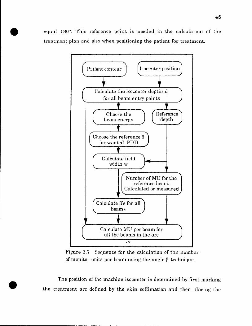
The treatment plan with the p angle concept can he separatc'd into
two parts: first, the calculation of the number of mOilitor UllltS Jlel' beam
needed ta compensate for the change in lsocenter depth as a l'und IOn of the
gantry angle and second, the calculation of the isodose dlstnhu tlon WI thin
the patient using the MU's per beam calculatcd prevlOusly
The first thing necessary in the calculatlOn of the do~e distribution
1S the patient contour. Also required is a hOrIzontal hne u~(~d as a
reference for the angular orientation of the patient A ref(~rence pOint on
the patient surface is defined by the entry point of the hearn pointing
directly down or in particular for the Varian Clinac 18 at. the gantry angle
45
equa! 180 Q
• This reference point is needed in the calculation of the
treatment plan and also V/hen positioning the patient for treatment.
Patient contour Isocenter position
Calculate the isocenter depths dl for aIl beam entry points
Choose the beam energy
Choa se the reference p for wanted PDD
Calculate field width w
Number of MU for the reference beam.
Calculated or measured
Calculate f3's for aIl beams
Calculate MU per beam for all the beams in the arc
. " Figure 3.7 Sequence for the calculation of the number
of monitor units per beam using the angle p technique.
The position of the machine isocenter is determined by first marking
the treatment arc defined by the skin collimation and then placing the
isocenter such that il represents the center of the ciI'de that lits tlll'
treatment contour best. This way of chùosing thl' isocl'Iltl'r enSlll"PS a dose
distribution as uniform as possible \Vith the isocentt'I' po~lt IOn and tilt'
patient contour, the depth of Isocenter is calculated for ail Sl1t'f~\l'l' l'nt l'y
points.
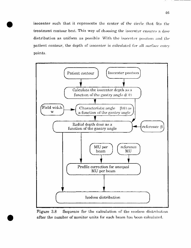
Figure 3.8
Patient contour Isocenter pllSlt 10 Il
Calculate the isocentcr dcpth as a functlOn of the gantry angle d( 0)
ChuracterÎsLtc angle I~W) as a function of the gantry angle
Radial depth dose as u function of the gantry angle
Profile correction for uncqual MU per beum
Isodose distribution
referenœ I~
Sequence for the calculation of the lsodose clistnhutloll
after the number of monitor units for each beam has he en calculated.
47
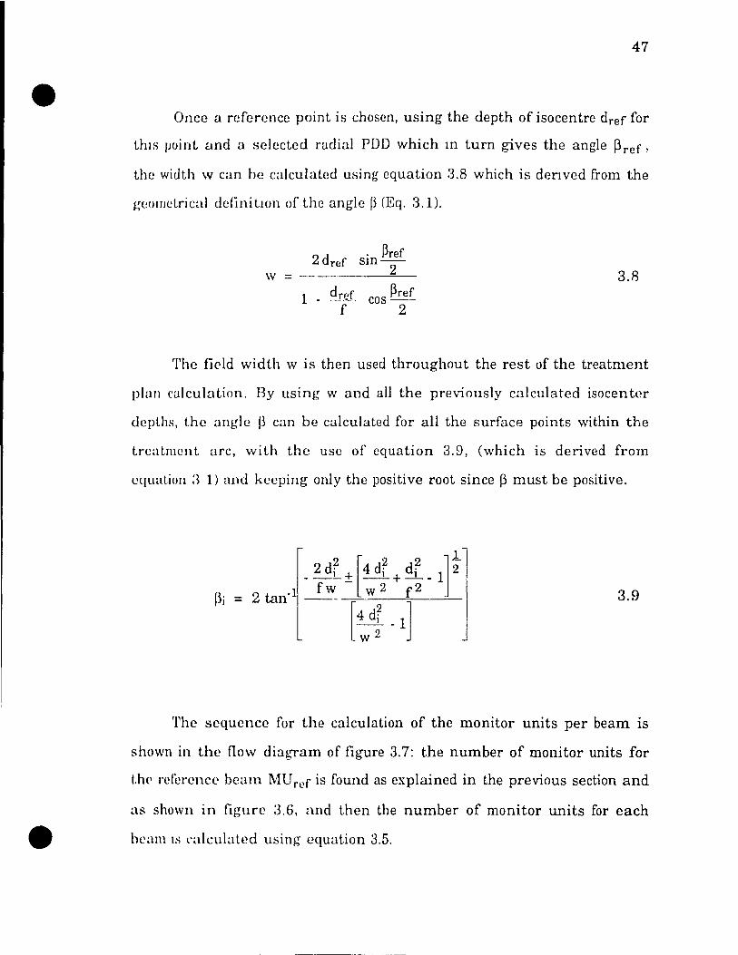
Once a reference point is chosen, using the depth of isocentre dref for
thls point and a scleded radial PDD which lJl turn gives the angle ~ref,
the width w can be calculated using equation 3.8 which is denved from the
~~e()llletrical definitlOI1 of the angle p (Eq. 3.1).
d . Pref w = __ ~~ef sm -2-
3.8 dref Pref 1 - cos--
f 2
The fi('ld \vidth w is then used throughout the rest of the treatment
plan calculation. By using w and ail the previously calculated isocenter
depths, the angle 13 ean be culculated for aIl the surface points within the
trcatmcnt arc, with the use of equation 3.9, (which is derived from
equatiol1 :3 1) and keeping oIlly the positive root since ~ must be positive.
2 [ 2 2 ]l _ 2 di ± 4 di + ~ _ 1 2
fw w 2 f2 .
-- [4 dT -1] w 2
3.9
'l'he sequence for the calculation of the monitor units per beam is
shown in the flow diagram of figure 3.7: the number of monitor units for
tJl(' referencl' beam MU ref is found as explained in the previous section and
as shown in figure 3.6, and then the number of monitor units for each
beam IS calclliated llsing equation 3.5.
48
Once the number of MU per bcam for aIl beams 18 known, t hl'
calculation of the isodosc distribution in the plmw l'on~:qdcrcd may lw
performed. Equation 3.5 g1Ves the MUs ncedcd tn Lompl'n~atl' t'Ol' t'hant~l'~
in the isocenter depth fùr cach bcam, but it assumes lwam:" wll h l'quai
monitor units and therefore, there must be a correctlUn fol' tlH' 1l11l'qU.l\
MU's of the beams (and this i8 why the MU's pel' lW;lm is l'l'quI l"l'd for t IH'
calculation of the isodose distribution). ThIs correction is a factor that
multiplies the isodose distribution calculatcd as If the t.rcatnH'l1t. hall l'quai
MU's per beam.
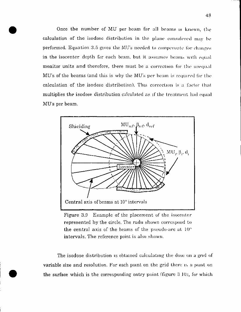
Central axis ofbeams at 10° intervals
Figure 3.9 Example of the placement of the Îsoccllter
represented by the circle. The radll shown correspolld to
the central axis of the beams of the pseudo-arc al, 10"
intervals. The referencc point i8 also shown.
The isodose distribution lS obtmned calculatmg the dose on a ~nd of
variable size and resolution. For each pomt on the grid there J!-' a pOlllt on
the surface which is the corresponding entry point (figure a 10), f(Jr which
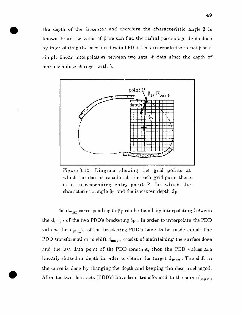
49
the dcpth of the isocenter and therefore the characteristic angle p is
known From the value of ~1 \'v'e can find the rachal percentage depth dose
by interpolatmg the measurcd radial PDD. This interpolation 1S not just a
simple linear interpolatIOn between two sets of data since the depth of
rrWXlffil'm dose changes wIth p.
P. corr,P " .'J •
point P P K
, depth .......
Il .... '
." dp .:\
~ .. n .. 1
1
1
~ ~ -----.. r. " 9 ' 'w.<. ... :: .. > ........ ::..~ ....... ;.. .. .. .... ""'.""'C <>'
Figure 3.10 Diagram showing the grid points at
which the dose is calculated. For each grid point there
is a corresponding entry point P for which the characteristic angle ~p and the isocenter depth d p.
'l'he d max corresponding to ~p can be found by interpolating between
the drnax's of the two PDD's bracketing pp . In order to interpolate the PDD
valtws, the limax 's of the brncketing PDD's have to be made equal. The
l'DI) transformation to shift dmax , consist of maintaining the surface dose
and the last data point of the PDD constant, then the PDD values are
linearly shiùed 111 depth in arder ta obtain the target d max . The shift in
the curve i8 done by changing the depth and keeping the dose unchanged.
After tht' two data sets (PDD's) have been transformed ta the same dmax ,
• 50
the target PDD curve c:m be culculated by s1mply interpolat.in~ hetw('t\l1
the two transformed PDD's.
The dose at the considercd gnd point can tlll'll hl' round t1~1l\~
equation 3.10, which 1S the PDD ut the grid point. multiplil'd by tlll' ll1vt'r~t.'
square law, the ratio of the ~'s, the ratio of the SUrf~lCl' d()~t's and t 11l'Il by
the profile correction factor KprùfY .The ratio of t1H' surt'acl' d()~l' I~ lH'l'dl'd
to scaie the dose since the i\.IU's per beum arc calculatl'd to l'l!Ualtzl' tlll'
surface dose everywhere on the trcated surfacl' bu t as IlIl'lltiOlll'd lwlill'l\
the surface dose will not be totally equalized and thal is t Ill' rl'a~()n Il lI'
including the profile correction in the calculation
D PDD (d)[f/-dref]2 ~p PDDrpr(ü)II
at grid point = P f' _ np ~ref PT)DP(-6) '-prof, P :1. 1 ()
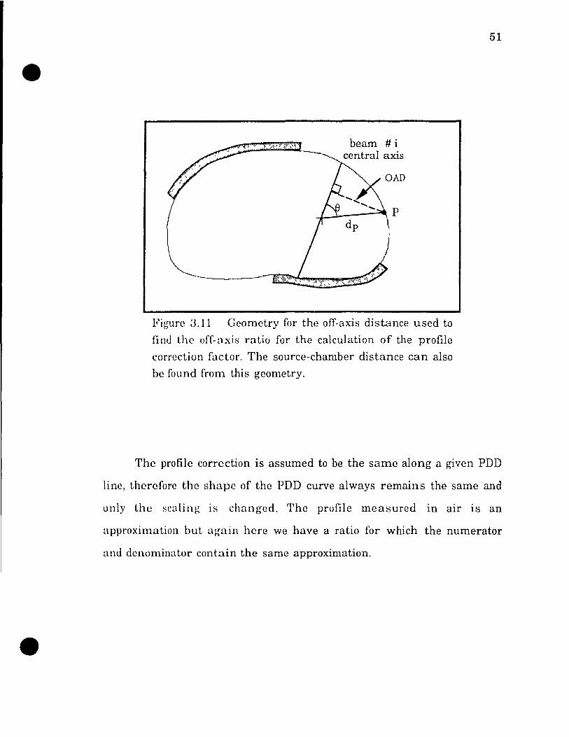
The profile correction factor (equation 3.11) is calculaicd fin' ail t.!H'
points on the patient surface using measured profiIc~ in air fiJr a series of
field sizes and source-chamber distances Figure 3.11 showf, the off-axis
distance for one bcam for the calculation of the off-axis l'aU, 1.
L [MU I OAR I (P)] K_ _ i (ail beams) .L~rof, P - '"
MUref L. :L11
1 (ail oeams)
Where OARI(P) is the off-axis ratIO from beam i to pOInt P on the
patient surface, MUi is the numbcr of monitor units for bcam i and MUrp (
is the number of monitor units for the reference bcam. 'l'he :'->um 1:'->
performed on the term for which the OAR i5 greatcr than !)(~J or up 1,0
beams ± 90° from the considered point P, whichever occurs tirs\"
------
beam # i central axis
.J..-..l----"""'\ P
Figure :3.11 Gcometry for the oIT-axis distance used ta
find the off-axis ratio for the calculation of the profile
correction factor. The source-chamber distance ean also
be round l'rom this gcometry.
51
The profile correction is assumed to be the same along a given PDD
linc, thereforc the shape of the PDD eurve al ways remains the same and
only the scaling is changcd. The profile measured . . . ln aIr lS an
approximation but again here we have a ratio for which the numerator
and denominator contain the same approximation.
•
52
Chapter 4
Evaluation of the angle ~ concept
4.1 Introduction
The evaluation of the angle ~ concept IS dont' by L'omp;u'ing a radl;l\
PDD calculatcd by a known treatment planning comput.er \VIth t111'
carresponding measured radial PDD used in the p algorit.hm lSf..'rt 1011
4.3.1). The isodose distributions produced with the 13 algonthm an' also
compared with isodose distributions mcasured wtlh film 111 a cylll1dncal
palystyrene phaLtom (Section 43.2). And finally, the ISO<!OSt' dl~tnbutlOlIs
calculated with the ~ algorithm, are venfied \Vith IIlP:lSUrelllt'lIts
performed using TLD's placed in a humanoid phantmll (Sedum ·1 :l.:n.
4.2 Input data
4.2.1 Angle ~ algorithm input data.
The radial percentage depth doses used for calculution of ISOÙOSP
distributions using the angle ~ pseudo-arc technique were obtained wlt.h a
30 cm diametcr cylindrical polystyrene phantom and the measlln~rn('nts
[21] were performed with thermolurninesccnt dosimetry C()mIH'is(~d of' 1,11"
rads (TLD-IOO rads, Harshaw Chemlcal Co, Cleveland, O/I) and a 'l'LI>
reader (Madel 2000, Harshaw Chcmical Co., Cleveland, (11) 'l'he i~oc(,l1ter
was placed at the center of the cylindcr and the numher of monitor UllIts
per beam given was equal for aIl the beams of the pseudo-arc No
secondary collimation was used and field width was dcfined hy the lower x
ray jaws.
53
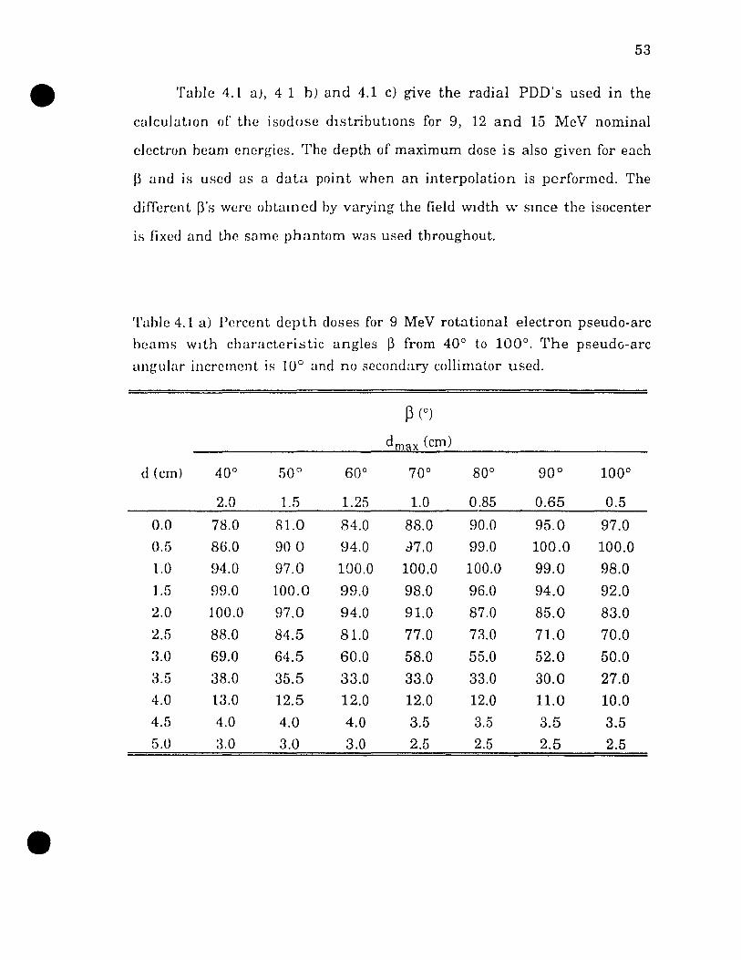
Table 4.1 a), 4 1 b) and 4.1 c) give the radial PDD's used in the
ca)cu)atIOn of' the isodose dlstributlOns for 9, 12 and 15 MeV nominal
electron beam energies. The depth of maximum dose is also given for each
~3 and is used as a data point when an interpolation is performed. The
different Ws were ohta1I1ed hy varying the field wldth \v smce the isocenter
is fixed and the same phantoffi was used throughout.
Tahle 4.l a) Percent depth doses for 9 MeV rotational electron pseudo-arc
bcams wlth characteristic angles p from 40° tü 100°. The pseudo-arc
angular incrcment is 10° and no sccondary collimator used.
p (0)
d mllx (cm)
d (cm) 40° 50 0 60° 70° 80° 90° 100 0
2.0 1.5 1.25 1.0 0.85 0.65 0.5
0.0 78.0 81.0 84.0 88.0 90.0 95.0 97.0
0.5 86.0 900 94.0 d7.0 99.0 100.0 100.0
1.0 94.0 97.0 100.0 100.0 100.0 99.0 98.0
1.5 ~)9.0 100.0 99.0 98.0 96.0 94.0 92.0
2.0 100.0 97.0 94.0 91.0 87.0 85.0 83.0
2.5 88.0 84.5 81.0 77.0 73.0 71.0 70.0
3.0 69.0 64.5 60.0 58.0 55.0 52.0 50.0 3 r: .tJ 38.0 35.5 33.0 33.0 33.0 30.0 27.0 4.0 13.0 12.5 12.0 12.0 12.0 11.0 10.0
4.5 4.0 4.0 4.0 3.5 3.5 3.5 3.5
5.0 a.o 3.0 3.0 2.5 2.5 2.5 2.5
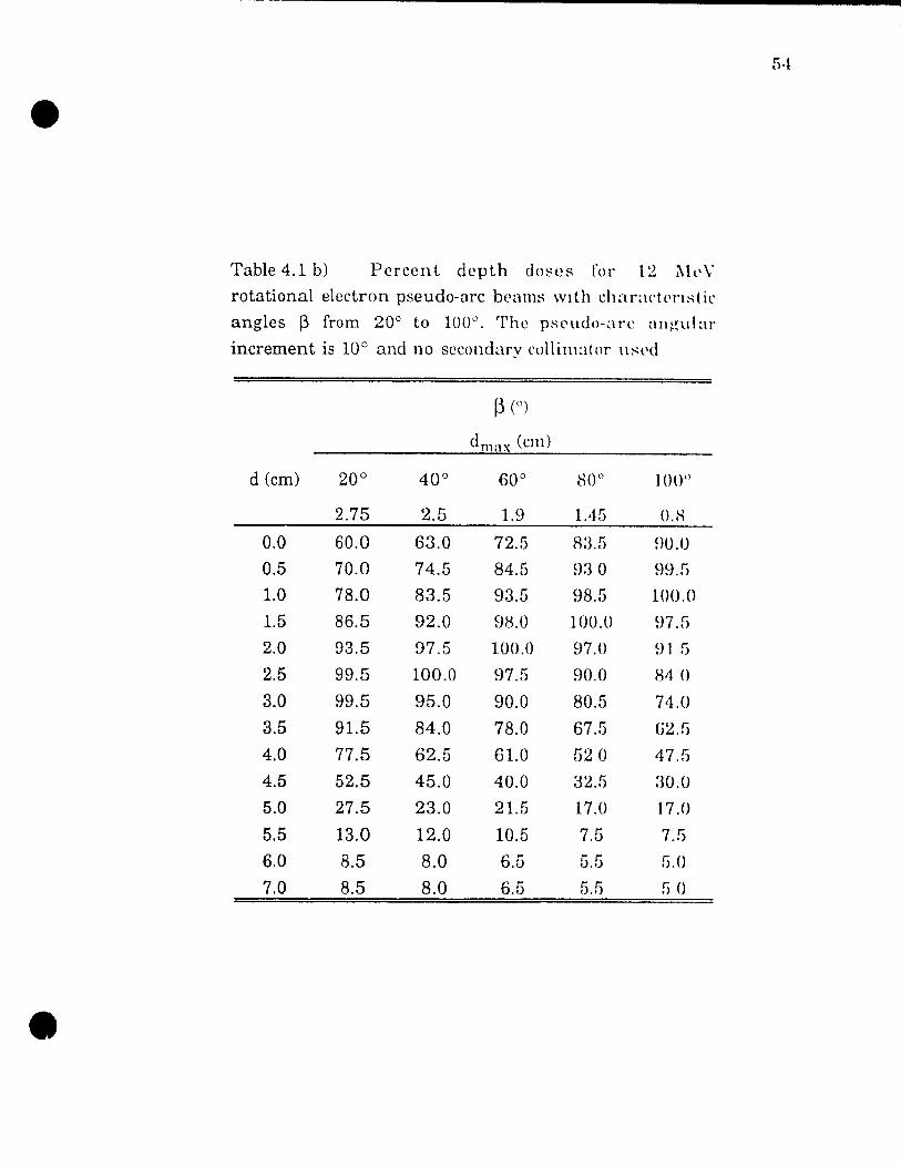
Table 4.1 b) Percent depth do::;es for 1:2 l\ll'\"
rotational electron pseudo-arc bl'ams \VIth charactrl"lst il'
angles (3 from 20° to 100e. The pseudo-arc an~~lllar
increment is 10° and no secondary collimator uSl'd
cl (cm)
0.0
0.5
1.0 1.5 2.0
2.5
3.0
3.5
4.0
4.5
5.0 5.5
6.0 7.0
2.75
60.0
70.0
78.0
86.5
93.5
99.5
99.5
91.5
77.5
52.5
27.5
13.0
8.5
8.5
2.5
63.0
74.5
83.5
92.0
97.5
100.0
95.0
84.0
62.5
45.0
23.0
12.0
8.0
8.0
dmax (cm)
1.9
72.5
84.5
93.5
98.0
100.0
97.5
90.0 78.0
61.0 40.0
21.5
10.5 6.5
6.5
80"
1.45
8:3.5
930
98.5
100.0
97.0
90.0
80.5
67.5
520
32.5
17.0
7.5
5.5
5.11
100"
O.H
DO.O
~)~U)
100.0
~)7.5
Dl G
840
74.0
G2.5
47.S
:30.0
17.0
7.5
5.0
50
55
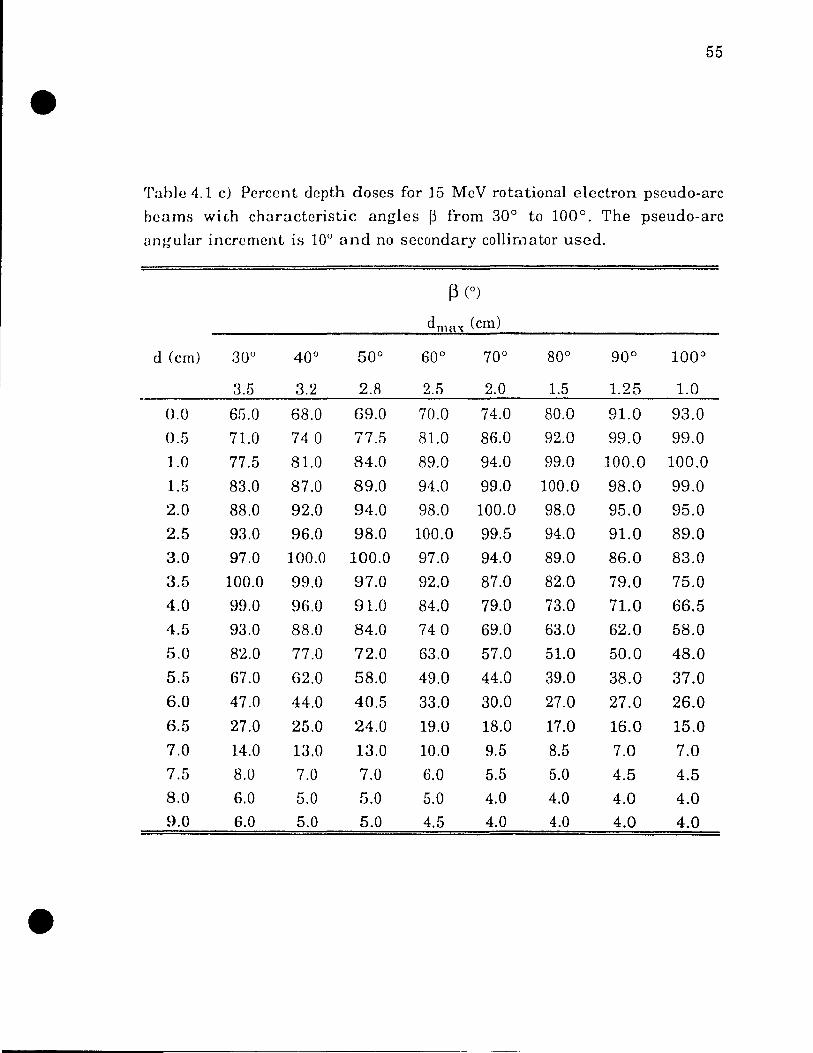
'l'ahle 4.1 c) Percent depth doses for 15 MeV rotational electron pseudo-arc
bcams wi(,h characteristic angles ~ from 30° ta 100°. The pseudo-arc
angular increment is lOU and no secondary collimator used.
~ (0)
dmax (cm)
cl (cm) 30° 40° 50° 60° 70° 80° 90° 100°
a.5 3.2 2.8 2.5 2.0 1.5 1.25 1.0
0.0 6S.0 68.0 69.0 70.0 74.0 80.0 91.0 93.0
0.5 71.0 740 77.5 81.0 86.0 92.0 99.0 99.0
1.0 77.5 81.0 84.0 89.0 94.0 99.0 100.0 100.0
1.5 83.0 87.0 89.0 94.0 99.0 100.0 98.0 99.0
2.0 88.0 92.0 94.0 98.0 100.0 98.0 95.0 95.0
2.5 93.0 96.0 98.0 100.0 99.5 94.0 91.0 89.0
3.0 97.0 100.0 100.0 97.0 94.0 89.0 86.0 83.0 3 r,: .<J 100.0 99.0 97.0 92.0 87.0 82.0 79.0 75.0
4.0 99.0 96.0 9l.0 84.0 79.0 73.0 71.0 66.5
4.5 93.0 88.0 84.0 740 69.0 63.0 62.0 58.0
5.0 82.0 77.0 72.0 63.0 57.0 51.0 50.0 48.0
5.5 67.0 62.0 58.0 49.0 44.0 39.0 38.0 37.0
6.0 47.0 44.0 40.5 33.0 30.0 27.0 27.0 26.0 6r,: .<J 27.0 25.0 24.0 19.0 18.0 17.0 16.0 15.0
7.0 14.0 13.0 13.0 10.0 9.5 8.5 7.0 7.0
7.5 8.0 7.0 7.0 6.0 5.5 5.0 4.5 4.5
8.0 6.0 5.0 5.0 5.0 4.0 4.0 4.0 4.0
9.0 6.0 5.0 5.0 4.5 4.0 4.0 4.0 4.0
5G
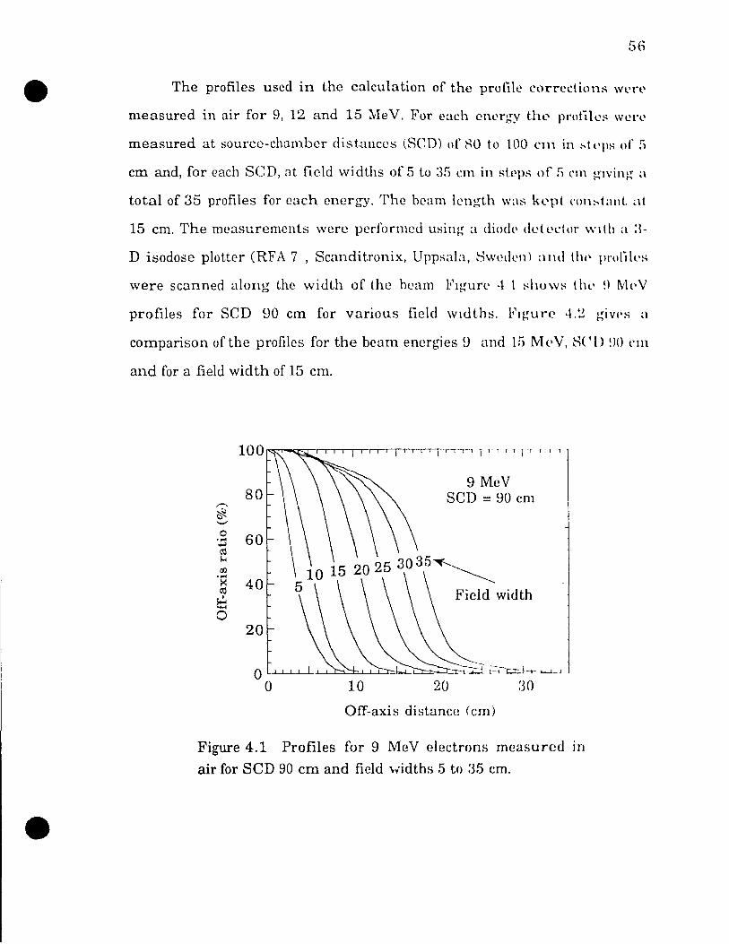
The profiles uscd in the calculation of the profile corrections Wl'rt'
measured in air for 9, 12 and 15 MeV. Fur each ellergy tht."' protiles wen'
measured at source-chamber distances (seO) of ~o tu 100 ClH in :-.tl'ps of !)
cm and, for each SCD, at field widths of 5 ta ~35 cm in steps of !) l'Ill g"lving- a
total of 35 profiles for each energy. The bcam length \Vas kl'pt l'()n~ta\lL at
15 cm. The rncasurernents were perfOfmetl using- a diodp dett.\ctol' wlth a :~-
D isodose pIotter (RFA 7 , Scanditrunix, Uppsala, Swecll'n) and thl' p\'oliks
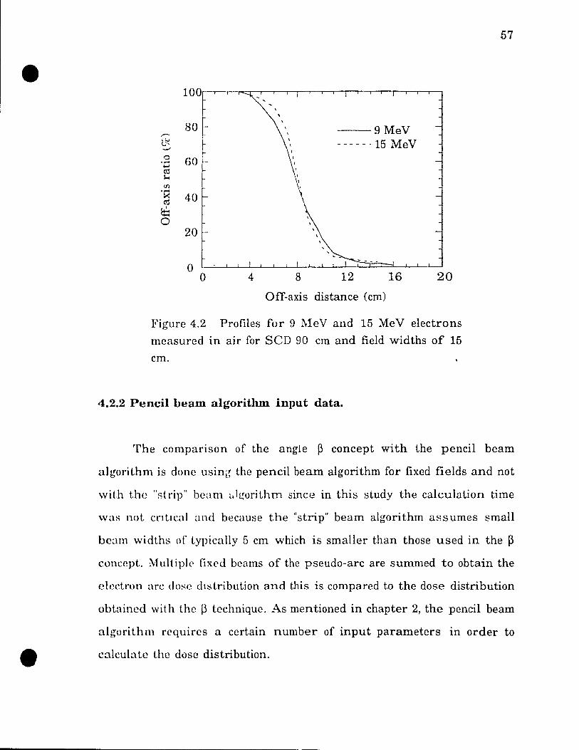
were scanned along the width of the beam FlgUt'l\ ·1 1 shows t 11l' !) l'vlpV
profiles for SCD 90 cm for various field wldths. Fq.~lln\ ,l.~ givp:-; a
comparison of the profiles for the beam energies 9 and Hi LVh\Y, SCl) !)() CIll
and for a field wid th of 15 cm.
80
o '.;j 60 ro 1-< rn
• po<
~ 40 ro ~ o
20
9 MeV SCD = 90 cm
10 15 20 25 3035~ 5 Field width
o ~"-,-'-L--L-J...-'--"---"'-'----'--"'---' o 10 20 :JO
OIT-axis distance (cm)
Figure 4.1 Profiles for 9 MeV electrons measurcd in
air for SCD 90 cm and field \fidths 5 to 35 cm.
------l
100
80 ,--. --9 MeV t~ ~
- - - - - - 15 MeV 0 60 ..... .... C'j s... <Il .r:::
40 ~ C'j
~ 0
20
0 0 4 8 12 16 20
Off-axis distance (cm)
Figure 4.2 Profiles for 9 1'.le V and 15 MeV electrons
IIlcasurcd in air for SCD 90 cm and field widths of 15
cm.
4.2.2 Penci} beam algorithm input data.
57
The companson of the angle P concept with the pencil beam
algorithm is donc usin~{ the pencil beam algorithm for fixed fields and not
wit.h the "strip" bcam olgorithm since in this study the calculation time
wus not cntlcal and because the "strip" beam algorithm assumes small
beam widths of typically 5 cm which is smaller than those used in the p
concept.. M uIt ipl(' fixed beams of the pseudo-arc are summed to ob tain the
elcctron arc dose chstribution and this is compared to the dose distribution
obtained with the ~ technique. As mentioned in chapter 2, the pencil beam
algorithm requires a certain number of input parameters in order to
calcula te the dose distribution.
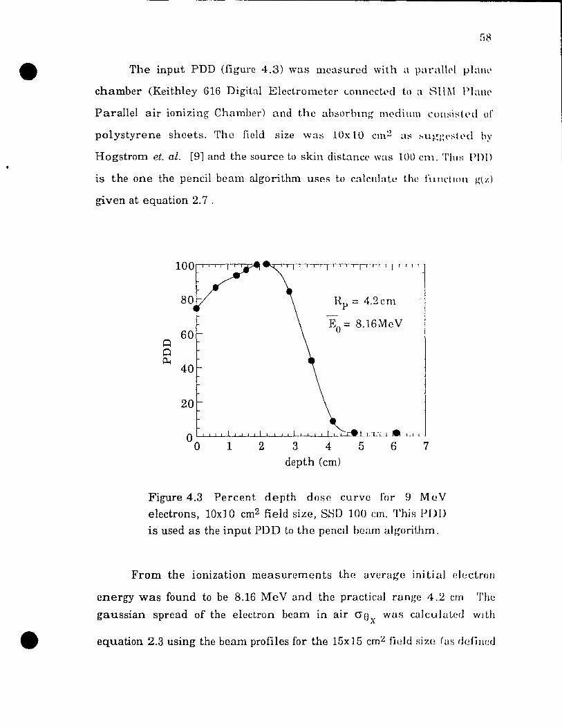
58
The input PDD (figure 4.3) wus lllcasurcd with a parallt'\ plalll'
chamber (Keit.hley 616 Digital Electrometcr l..onncctcd tn a SIl1\1 Planl'
Parallei air ionizing Charnber) and the ubsorblllg medium COJl:-;iskd or polystyrene sheets. The field size was lOx 10 cm 2 as :-,ugg(,:-;tl'd hy
Hogstrom et. al. [91 and the source tü skin distancC' was 100 Clll. 'l'ills PD\)
is the one the pencil bearn algorithm uses tü calculatc the functllll1 ~(z)
given at equation 2.7 .
100 1 Iii i 1 1 rr,T 1 1 1 111
80 Rp = 4.2cm
60 Eo= 8.16MeV
Cl Cl P-4
40
20
00 1 1 Il 1 1 1 1 1 1 L.L...L.1:::rrCl-. 1-J L
1 2 3 4 5 6 7
depth (cm)
Figure 4.3 Percent depth dose curvc for 9 M eV
electrons, lOxJ 0 cm2 field size, SHD 100 cm. 'l'his PDO is used as the input PDD to the pencli beam algorithm.
From the ionization measurements the average ini ti al electroll
energy was found to be 8.16 MeV and the practical range 4.2 cm The
gaussian spread of the electron bcam in air (j8 x was calculaLr~d wll,h
equation 2.3 using the beam profiles for the 15x 15 cm2 fil~ld sizc (as defill(~d
59
by the x-ray Jaws) and source to chamber distances 95 to 120 cm in steps of
fi CIn. This beam profile was measured the same way as explained in
section 4.2.1. The resultIng <J0x was 47.6 milliradiants. The15x15 cm2 field
size used here was chosen as Ull field size closest tü the field width giving
an angle f3 of 80° for an isocenter depth of 10 cm which is 13 9 cm. A
cylindrical phantom of 20 cm in diameter was assumed ln the cornparison.
The la~t parameter required hy the pencil bcam algorithm, the
source-to-collimator distance, was set at 30 cm. This 18 the distance from
the phy~lcal source to the lower edgc of the lower jaws; sinee in the ~
techmque the secondary collimation is generally omitted, the distance
choscn is adequate for UH' purposc of comparison of models. This distance
also dPll'rnllne: .. the air gap WlllCh contl~butes to the electron beam spread.
4.3 Evaluation
4.3.1 Pencil beam calculation.
A 20 cm diameter cylindrical phan tom was also assumed in the
simulation with the GE Target 4 treatment planning system and a
no mi nal elect.ron beam encq,')' of 9 MeV was used. The field size required to
obtain a I~ of SOU was calculatcd as 13.9 cm and this field size was used
throughout tlH' plan The fixed beams were defined at every 10° (gantry
angle) creat mg a full ~H10° pseudo arc.
The radial PDD obtained from the pencil beam algorithm (GE
Target 4 soft\'.'are) gave a d max of approximately 1.6 cm which is smaller
t.han the 2.2 cm oÎ the single fixed beam input PDD shown in figure 4.4 .
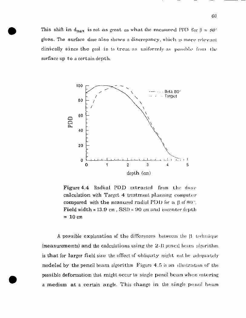
60
This shift in dmax is Bot as great as what the n1casuH'd l'nI) for ~~ ::: ~O"
gives. The surface dose also shows a discrepancy, which IS mort' rt'll'v:1nt
clinically since the goal is Lo treat as unifonnly as posslhll' t'rom t Ill'
surface up to a certain depth.
depth (cm)
Figure 4.4 Radial PDD extracted frorn thl' d()~w
calculation with Target 4 treatment planning comput(!r
compared with the measured radial PDU fè)r a I~ or HO".
Field width = 13.9 cm, SSD = 90 cm and isocpntpr <IepLh
= 10 cm
A possible explanation of the differences hetween the I~ tp('hll i qlW
(measurements) and the calculations using the 2-D pencIl beam ;jll~(JrithJJl
i8 that for larger field size the efTect of obliqUlty might.. not. be ad(~qlla Lely
modeled by the pencil boam algorithm Figure 4.5 is an dlllst.nltlOn of the
possible deformation that might occur to single pencil beam when (!/llering
a medium at a certain angle. This change in the single penc:il ~H!am
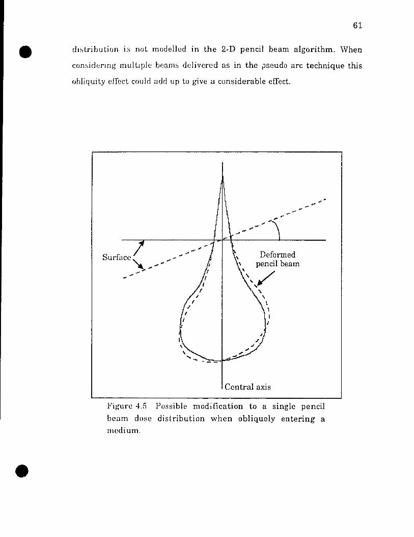
61
ùlf-llribulion i:.; not modelled in the 2-D pencil beam algorithm. \Vhen
conf-liù(~rlng multiple bcamf-l delivercd as in the pseudo arc technique this
ohliquity cffecl could add up to give a considerable effect.
.. ,. ......
Defarmed \ pencil beam
\ ... / " \.
\ 1. 1 1
1
Central axis
Figure 4.5 Possible moddication ta a single pencil
bcam dose distribution when obliquely entering a
medium.
4.3.2 Measurements with film.
The procedure followed to expo~e and obtain tlll' dose distnhlltion
from a therapy verification film (XV2 , Kodak Inc., Roche:ster, NY, U.8 A) is
as follows;
i) The film was eut in a darkroolll to fit on a ;W l'Ill (h:\Ilwt.l'1"
polystyrene phantom. The film's envelopc was kept. in Ot'dl'!" to protl'd. tilt'
film from the Cherenkov radiation that occur in Hw absorhin~ IllC(IIUIll, in
this case polystyrene.
ii) The film was then fixed on one sluh of the phantoill \VII Il ;1 slllall
plece of tape and sandwichcd with the (lther slab of' t1w llhallt.olll l1~illg
opaque plastic tape (black clectncal tape) the two part:-- or tilt' phantolll
were taped and tightly cIamped togethl'r with large C-clamp:-, !'l'ad, fi l!llll
thick, \Vas used as a tertiary collunator to ~hicld the low('I' h,dl' of' t.1ll'
phantom and to eliminate the shlClchng l'lIed of UlP clamps
iii) The cylinder was then posltionc·d wlth t1H' iSOC(!lltP!' cOIllCHlrllg
with the geornctric center and the film wa~ eXjJoseù wlth LIli' rf'qlIln'"
number of monitor units per beam to conform wIth the simulat.1011
iv) The film was processed \Vith an auLomatJc pro('('!->sor alld Ul<'
optical density \Vas measured using a scanni n~ densl LOIlll'Lpr WI th a Il
aperture of 0,5 mm. The net optical demilty (measured op!'lc:!1 dPIlSlty
minus base plus fog) was normahzed to 100% at the mén.llllUllI dt'fl!->Ity
value along the reference radii.
Four isodose dIstributions calculated \Vith the f3 ulgorrthm compared
with isodose distributions measured with film in a cyhndrrcul p()ly~tyrene
phantom will be illustrated below in figures 4.6 to 4.9.
63
The number of monitor UI.tÏts given for the cases shawn in figures
4.6 tü 4 9 were chosen so that the optical density remained entirely within
the linear region of the H&D curve of the film. For the XV2 film [5] the
Iinear reglOn corresponds to doses less than 50 cGy. This facilitates the
procedure Slllce the relative dose distnbution c::m be obtained directly
l'rom the optlcal density measurement wlthout any conversion function.
A cornmon point ta the four examples given here is that the
shielding at the surface of the phan.om is not modeled in the P concept
treatment planmng pragram, but the surface dose changes mostly within
2 to :3 cm from the edge of the shielding and this can be taken into
consideration wlwn the treatment arc is determined. The difference in
dose penetI atiOI1 is very evident with the dose distributions shown below.
The s.1ift in d max can easily be seen between the Ws of 50 0 and 80 0
and the calculatlOns directly prediet this shift. IL is important to
remember that with electron arc therapy the most uniform distributions
are obtained when the geometry lS as close to a circle as possible and this
can generally he :"atJ:·,fied wlthm a normal treatment arc sueh as an arc
contuined wi thin the left or right si de of the chest wall. With such
geometrics, the modeling using measured radial PDD with circular
symmetry cun be used with confidence.
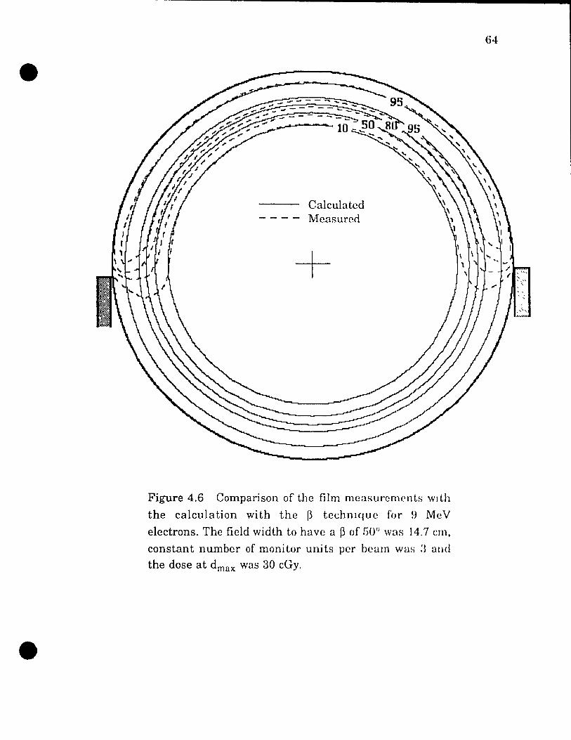
•
Calculatcd l'vlcasured
+
Figure 4.6 Companson of the film rneasurcnH.'nLs WI th
the calculation with the P technique for 9 MeV
electrons. The field width to have a P of GOG was 14.7 cm,
constant number of monitor units per bearn was :~ and
the dose at dmax was 30 cGy .
H4
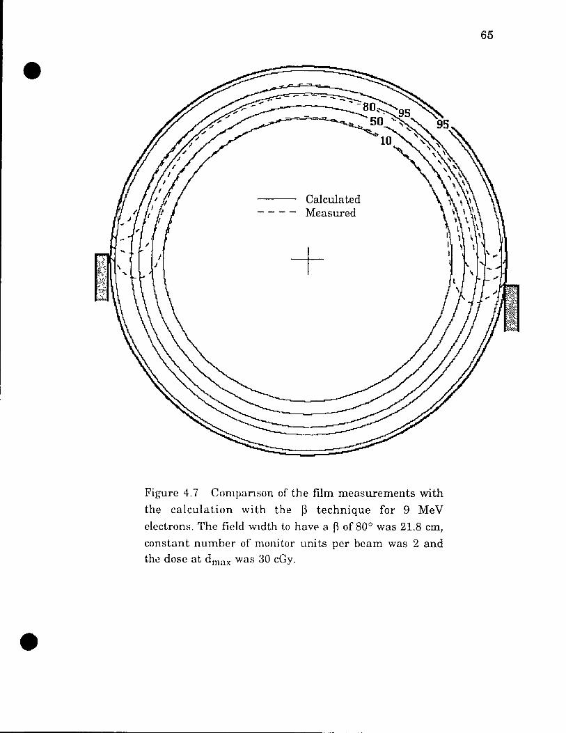
Calculated Measured
+
Figure 4.7 Companson of the film measurements with
the calculation with the ~ technique for 9 MeV
electrons. The field wldth to havp a 0 of 80° was 21.8 cm,
constant number of monitor units per beam was 2 and th~ dose at d max was 30 cGy.
65
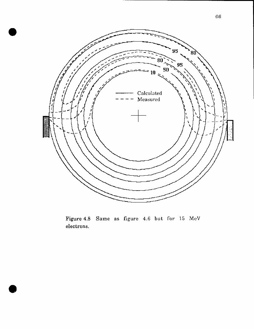
.. ------------------------------------------------------------------------------~
Calculated Measured
+
Figure 4.8 Same as figure 4.6 but for 15 MeV
electrons.
6(1
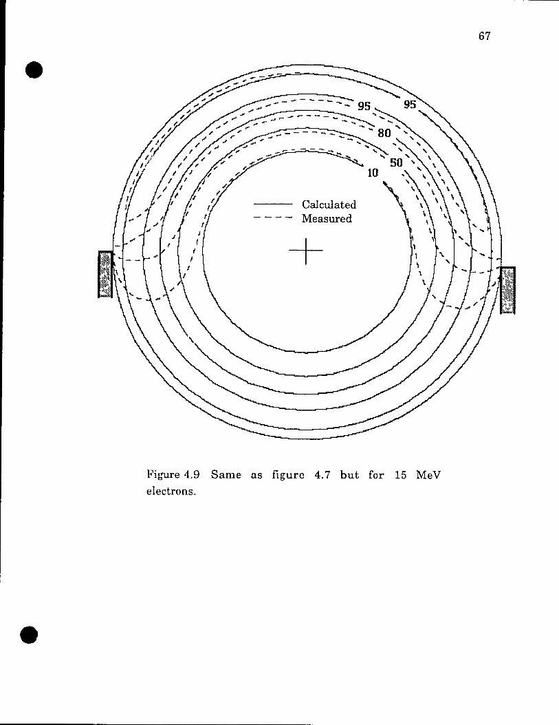
Calculated Measured
+
Figure 4.9 Same as figure 4.7 but for 15 MeV
electrons.
67
68
4.3.3 Humanoid phantom.
The isodose distribution shown in figure 4.10 was calcllbted ll~in~
the treatment planning program developed for thls thesls and it
corresponds to the experimental set-up used by Pla et. al. [211 . This was
calculated here as one test for the program SInce the distnbution l"l'fl'ITl'd
to had been verified with TLD llH'aSllremC'nts The progralll calcul:l !,lOns
are practically identical to that of Pla et. al [21] and t.he \,pry ~Illall
differences can be attribllted to the different calculatioll n'sol ut IOn For
this study the dose was calculated on a grid with 1 mm resolution \VIllie III
the case of Pla et. al. the dose was calculated on tllP hne::; IWJ"pt'Ildiclllar to
the surface beginning at the central axis entry points of' UH' pseudo arc
beams which are at 10° intervals. For a geometry such as in figuJ"l' ·1 10,
where the isocenter is placed at the vicmIty of the center of a transverse'
slice, the resulting surface dose is fairly uniform.
The computer programme calculates the number of MU per heam,
the corresponding Ws, the surface dose corn'cLed for uncqllal monItor
units (profile correction), and the isodose distnbutIOn. The MU pe,. IH'am
are the MU's that are used when the treatment IS given tu the patient.
The effect of bolus may also be taken into comiHlcratlon hy the
computer programme simply by includiüg the bolus in the patient contour.
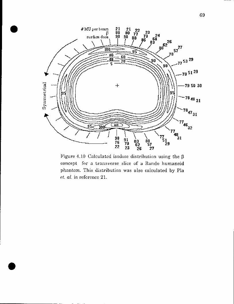
#MUperbeam 21 ~ 80
surface dose 90
\
\ 91 83 70 62 23 26
26
69
-7950 30
--- 78 48 31
""'-7847 31
"-7746
\. """77 32 '\ 77 48
51 31 29
Figure 4.10 Calculated isodose distribution using the ~
concept for a transverse slice of a Rando humanoid
phantom. This distribution was aisa calculated by Pla
et. al. in refcrence 21.
Chapter 5
Conclusions
70
Electron arc therapy i8 the modality of choicc 111 the trl'atnll'nt. of
certain large 8uperficial tumors following curvcd surrace~. llowl'vl'I' 1I1l'
treatment planning is complicated and the paLient prl'paration is t.inw
consuming which discourages the use of this t.l'chniquc by .·adiotlwrapy
centers,
There are basically three methods for calculat.i ng l'ledrol1
pseudoarc isodose distribut.ions using: a) measured angular dosl' pro{ilps
and radial depth dose, such as Leavitt et al. [lGI have proposl'd, hl a Pl'I1('!l
beam algorithm modified for electron arc t.hcrapy [(j 1; and r) tilt' anglp-I\
concept developed at lVIcGill [21]. The first two an' g-l'Ilerally u:wd wll Il a
fixed field width, usually about 5 cm, and bolus t.ü control holh Uw surf'ac('
dose and treatment depth. "Vi th the angle-~ t.eChl1lqlH.', t.he fil'ld sizl' is
calculated from the depth of lsoecnter and the sl,lecleJ radiai 1)(·rcl'llI.age
depth dose. In this case bolus may be used tn reduce t.he dos(' t.o IIILprnal
structures but the shielding required 1S more elaboralc due lo the largC'r
field width, normally about 15 to 20 cm,
The p-coneept's fundamental feature 18 the cslablishnH'nl of il
simple relationship between depth of isocentrc, field wldlh, :lnd <lllgie Il,
with two special characteri8tics: a) a given angle 11 can tH' o!lt:llllt'd l'rom
different combinations of field width and depth of' 1f,OCentl'c, and h) (iH' C':!ch
different PDD there is a unique angle p which cha"aclenz(!s t.ill~ PDD,
The implications of these two special propertws of the angl(~ r~ cone(~pl are
very important clinically: prior to a treatment the radioli1craplst, ba~(~d 0/1
the depth of treatment, ean select the best electron cneq~y and PDU,
71
which in turn gives the angle ~ to be used. Once 0 is known, the tre:atment
geometry, i.e., selection of isocentre and field width, can be defined to
provlde the requef-,ted 13 and therefore the requested radial PDD. If the
placement of the Isocenter 18 such that a good circular geometry is
obtnined, the angle p will only vary slightly along the treatment contour
thcreforl' producmg the required radial PDD with only minor variations.
The POD 18 less sensitive tn variations in 0 for larger 13 angles, of about
HO", than IL is for' smaller ones of about 40°. Thus larger 0 angles render
more uniform do!->c dlstnbutlOIls along with a higher surface dose which is
usually a treatment. rcqUlrement.
With the 0 techmque the inclusion of inhomogeneities can only be
donc, strict.ly spealong, for eylindrical geometries.
As wc have seen, the pencil beam algorithm does not seem to predict
correctly thc measured shlft ln dmax Bor the surface dose, while the 13
technique accounU:; for both properly.
One possible improvement for both calculation techniques would be
to join them in sorne way that would incorporate the best of both, namely
the ~ technique's ability to prcdict PDD's, and calculations that include
CT#'s as cloes the pcncil bcam algorithrn. The way it may be possible to do
t.his is by using the r.~ concept as F\ PDD generator that would give the PDD
to bl' used in the calculaliol1 of the fudging function g(z) of equation 2.7 .
Each stnp beam could be calculated with a new g(z) that would reflect the
Îsocenter dppth <.lt the reqUlred position. Also with this merging, a
treatmcnt rl'quiring multiple energies could be done the same way with
the radial PDD's for the particular energies.
• 72
The computer program developed for this work calcula tes isodnst'
distributions disregarding the efTect of the tertiary collimation placl'd
directly on the patient's surface; with this approxlInation. tlw distributIOn
is only valid starting from about 2 cm from the ('tige of the ~hü'ldlllg 'l'he
patient contour can be entered in minutes and t hen the isocl'nt l'r l'an \w
chosen with the help of adynamie circle (t.he l'l l'cl l' chan~es whel1 the
isocenter is moved within the patient contour) which gU1dl'~ t Ill' uspr fol'
the best fitting circle ta the patient treated contour. 'l'Il(' dlOSl'1l l:-'lH'l'nt.t'r
can be changed at any time tü optimize the dose distribution lllltii LIll'
geometry of the treatment bccorncs satisfactory The prog-ram outpub lIll'
treatment plan which consist of the number of monl tOI' uni ts Ill'r Iwam
required by the ~ technique and the correspondmg I~()d()~t\ dlstnbutlOIl.
Sinee this program was written for the Macintosh eornputer the llspr
interface or its appearance to the user is such that cverything- ('an be donc
visually and interactively.
73
References
1. ,J. Becker, G. Weitzel, "New forms of moving radiation from a 15 MeV
Siemens bctatron. StrahlentherapIe 101, 180-190 (1956).
2. B. E. Blackburn, "A pracbcal system for electron arc therapy",
Proceedings of the symposium on electron dosimetry, 295-314,
( 1981).
:t A. L. Boyer, G. D. Fullerton, ,J. G. Mira, "An electron beam pseudo
arc technique for irradiation of large area of chest wall and other
curved surfaces", Int. J. Radiat. Onco!. Biol. Phys. 8, 1969-1974
( 1982).
4. r. Bruinvis, "Electron Beams in radiation therapy: Collimation,
dosimctry and treatment planning", thesis, Drukkprijelink\\<ijk B.V.
- Utrecht (HJ87).
5. M.D.C. Evans and L.J Schreiner, "A simple technique for film
dosimetry" , RadlOthcrapy and Oncology 23, (1992).
6. K. R. Hogstrom, R. G. Kurup, A. S. Shiu, G. Starkschall, "A two
dimensional pencil bcam algorithm for calculation of arc electron
dose distnbutiolls", Phys Med Biol. 34, 315-341 (1989).
7. K. R. Hogstrom, n. D Leavitt, "Dosimetry of arc electron therapy",
Proceedings of the AAPM 1986 St~~mer School, 247-276 (1986).
8. K. R. Hogstrom, "Evaluation of electron pencil beam dose
calculation", Radiation Oncology Physics-1986 (Medical Physics
Monograph 15), 5~32-557 (1986).
9. K. R. Hogstrom, M.D. !vlills, P. R. Almond, "Electron beam dose
calculations", Phys. Med. Biol. 26, 445-459 (1981).
10. K. R. Kase, B. E. Bjarngard, "Bremsstrahlung dose to patients in
74
rotational electron therapy", Radiology 133, 531-532 (lH7~)).
11. F. M. Khan, F. C. Deibel, A. Soleimani-Mel~ooni, "Obhqmt.y
correction for electron beams", Med. Phys. 12. 74H-7fi~l (l~)H[))
12. F. M. Khan, G. D. Fullerton, J. M.-l? Lee. V C l\lool"l'. S. II Ll'vitt.
"Physical aspect of electron-beam are therapy". Radiology 12·1. ·t97-
500 (1977).
13. D. D. Leavitt, J. R. Stewart, J. H Moeller, L. Early, "Optimization or
eleetron are therapy doses by multi-vHm' colh mator l'on t roi", lllt. ,j
Radiat. Oneol. Biol. Phys. 16, 489-4H6 (198D)
14. D. D. Leavitt, "Multileaf collimatIOn in elect.roll an~ t.hl'rapy",
Proeeedings of the 12th Varwn Users' met,ting", fi:3-G7 (19HH).
15. D. D. Leavitt, L. M Peacock. F A. Glbbs,.I l{ Stt'wart" "EI(,l'trol1 <Ife
therapy: PhYRical mea~;urement and tn',lt.nH'1l t. pl (11111111 /.!
techniques", Int. J. Radiat. Oneol. Biol. Phys. Il, DH7-~)()9 (I!H.;r;).
16. S. C. Lillicrap, P. Wilson, ,1. W. Boag, Phys. Mpù. Bio!, 2(}, :W-:IH
(1975).
17. E. Mah, J. Antolak, J. W. Serimger, J. J. Battlsta, ''I~xperilllt'Iltal
evaluation of a 2D and 3D electron pencil heam algorl thrn", Phy~·i.
Med. Biol. 34, 1179-1194 (1989).
18. E. Mah, J. Battista, J. Scrimger, "AcquisitIOn and display of
radiation dose distributions using mieroeomputcf technolo~y", MI!d.
Phys. 15, 924-929 (1988).
19. A. E. Nahum (editor), "The computation of do~c ùl~tnbuti(Jns III
electron beam radiotherapy", UMEA University Cl9Hfi).
20. L. M. Peacock, D. D. Leavitt, F. A. Gibbs, ,I. H.. Stcw<Jrt, "Electron are
therapy: Clinical expenence with chest wall IrraùIation", InL ,1.
Radiat. Oncol. Biol. Phys. 10, 2149-2153 (984).
75
:l1. M. Pla, E. B Podgorsak, C. Pla, C. R. Freeman, L. Souhami, J.
Guerra, "Physlcal aspects of the angle-~ concept in electron arc
thernpy", Int. ,] Radiat Onco!. Biol. Phys. 21, 1331-1339 (1991).
2:l. M Pla, r~. B Podgor~ak, C. Pla, "Electron dose rate and photon
eontamÎnatlOn III electron arc therapy", Med. Phys 16, 692-697
( 19R9).
:l;3. M. Pla, C. Pla, E. B. Podgorsak, "The influence of beam parameters
on percentage depth dose in electron arc therapy", Med. Phys. 15, 49-
55 (1988).
24. .J. Rassow, "On the telecentric small-angle pendulum therapy with
high electron energy betatron", Radiology 133, 483-489 (1972).
25 D R. Ruegscgger, S. D. Lcrude, D. Lyle, "Electron-beam arc therapy
111-iing a high energy betatron", Radiology 133, 483-489 (1979).