Promotion, Turnover and Compensation in the Executive Market · · 2015-07-14Promotion, Turnover and Compensation in the Executive Market ... Miller (Carnegie Mellon University)Promotion,

Promotion, Turnover and Compensation in the ExecutiveMarket

George-Levi Gayle, Limor Golan, Robert A. Miller

Carnegie Mellon University

June 25 at Cowles Conference

Gayle, Golan, Miller (Carnegie Mellon University)Promotion, Turnover and Compensation June 25 at Cowles Conference 1 / 36

IntroductionWhat are executives paid for?

CEOs are paid more than executives in lower ranks.

Average tenure of a CEO is �ve years.

They are mainly promoted internally.

Is promotion to CEO a reward for excellent service at lower ranks?

The income volatility of CEOs is also much higher.

Rent from human capital or risk premium?

Are there non pecuniary bene�ts?


IntroductionWhat we do: develop and estimate structural model

Formulate a dynamic model where there is:1 Moral hazard and incentive concerns2 Human capital, �rm speci�c and general3 Job turnover stimulated by demand from �rms for a mix of executivetalent and idiosyncratic (private) shocks to executives.

Identify non pecuniary bene�ts of jobs, human capital, risk premium,span of control.

Estimate model and compute importance of factors above.


IntroductionBackground literature

There is a growing literature on estimating structural models ofcontracting.

See Ferral and Shearer (99), Margiotta and Miller (00), Dubois andVukina (05), Bajari and Khwaja (06), D�Haultfoeviller and Fevrier(07), Einav, Finkelstein and Schrimpf (07), Nekipelov (07), Gayle andMiller (08a,b,c).

In related work Gibbons and Murphy (92) test implications of optimalcontract with career concerns, and Frydman (05) presents evidence onturnover and general human capital.

There is little empirical work relating career hierarchies to humancapital, promotion and job turnover.

See Baker Gibbs and Holmstrom (94) for a case study of one �rm.


IntroductionOutline of this talk

Brie�y describe the data.

Develop a structural model.

Discuss identi�cation and estimation.

Present preliminary results from structural model.


DataSources

S&P ExecuComp database.

Compensation and title on top 5 paid executives (1992-2006).

30,614 executives with at least one year of data.

2818 �rms S&P 500, midcap, smallcap.

Matched sample with background data from "Who�s Who".

Matched 16,300 executives in 2100 �rms.

Compensation data:

Direct compensation (cost to shareholders): salary, bonus, value ofrestricted stocks and options granted, retirement and long-termcompensation schemesTotal compensation (relevant for manager): also include wealthchanges from holding �rm options and stocks


DataRanks and transitions

We constructed a life-cycle based hierarchy of 7 ranks:Rank 1 includes ChairmanRank 2 includes CEORank 4 includes COORank 5 includes Senior VP

See Gayle, Golan and Miller (2008) for details.Most executives do not move in any given period.Internal promotion by one rank is the most common job transition.99% of Rank 2 executives are not demoted.They occur morefrequently at lower levels, 5% in Rank 3, 7% in Rank 4.There is more exit than entry in lower ranks.There is more entry than exit at higher ranks.A small percentage of transition involves turnover.Movers are more likely to change ranks than stayers, with promotionmore likely than not below Rank 2.


DataJob mobility within the �rm

Table 2a: Internal TransitionsRANK 1 RANK 2 RANK 3 RANK 4 RANK 5 RANK 6 RANK 7 Size exit %exit

RANK 1 88 6 3 1 1 0 0 3995 487 12

RANK 2 4 95 0 0 0 0 0 20150 929 5

RANK 3 3 14 78 3 1 1 0 6272 1370 22

RANK 4 1 2 3 86 4 2 1 19359 2624 14

RANK 5 1 1 2 7 85 2 1 15781 2356 15

RANK 6 0 0 1 6 6 85 2 14646 2248 15

RANK 7 0 1 1 6 3 7 81 5581 1035 19

entries 1303 1872 1447 2634 1981 1086 726

%entries 33 9 23 14 13 7 12


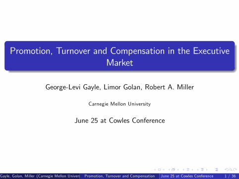
DataJob mobility between �rms

Table 2b: TurnoverRANK 1 RANK 2 RANK 3 RANK 4 RANK 5 RANK 6 RANK 7 Size Size Transition

Moves Rank Rate

RANK 1 52 36 8 4 1 0 0 165 3995 4.1%

RANK 2 19 58 9 5 7 1 0 389 20150 1.9%

RANK 3 10 40 26 14 9 1 1 140 6272 2.2%

RANK 4 3 21 7 40 12 11 5 281 19359 1.5%

RANK 5 2 36 10 14 34 3 1 211 15781 1.3%

RANK 6 0 9 8 30 8 34 10 130 14646 0.9%

RANK 7 2 13 4 30 6 19 26 53 5581 0.9%

Total 188 496 141 244 160 96 44 1369 85748 1.6%


DataDemographics on executives

Table 4: Executives CharacteristicsAge, Gender, Education and Experience

Variable Rank1 Rank2 Rank3 Rank4 Rank5 Rank6 Rank7

Age59.6

(9.8)

55.7

(7.6)

52.4

(8.0)

52.0

(8.8)

52.8

(10)

52.4

(10.3)

52.2

(11.2)

Female 0.02 0.02 0.03 0.05 0.06 0.06 0.05

No Degree 0.25 0.21 0.25 0.21 0.21 0.17 0.21

MBA 0.24 0.26 0.23 0.27 0.19 0.18 0.22

MS/MA 0.16 0.17 0.17 0.19 0.21 0.21 0.21

Ph.D. 0.15 0.15 0.14 0.13 0.21 0.27 0.17

Prof. Certi�cation 0.15 0.14 0.15 0.22 0.24 0.37 0.30

Executive Experience22.3

(13.0)

19.8

(10.5)

16.1

(10.7)

15.9

(11.0)

16.6

(12)

16.5

(11.7)

16.9

(11.7)

Tenure17.1

(13.5)

15.1

(11.7)

13.7

(11.4)

13.8

(11.2)

14.1

(12)

13.7

(11.0)

14.2

(10.8)

Gayle, Golan, Miller (Carnegie Mellon University)Promotion, Turnover and CompensationJune 25 at Cowles Conference 10 /

36

DataExecutive movement and compensation

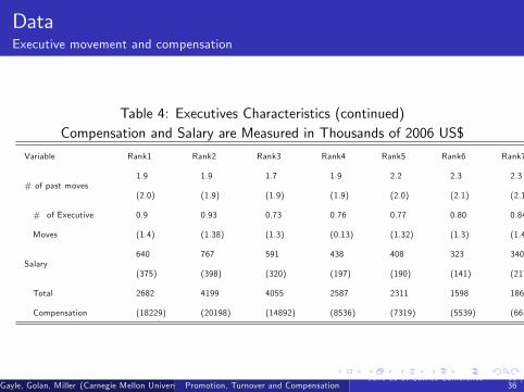
Table 4: Executives Characteristics (continued)Compensation and Salary are Measured in Thousands of 2006 US$

Variable Rank1 Rank2 Rank3 Rank4 Rank5 Rank6 Rank7

# of past moves1.9

(2.0)

1.9

(1.9)

1.7

(1.9)

1.9

(1.9)

2.2

(2.0)

2.3

(2.1)

2.3

(2.1)

# of Executive

Moves

0.9

(1.4)

0.93

(1.38)

0.73

(1.3)

0.76

(0.13)

0.77

(1.32)

0.80

(1.3)

0.84

(1.4)

Salary640

(375)

767

(398)

591

(320)

438

(197)

408

(190)

323

(141)

340

(217)

Total

Compensation

2682

(18229)

4199

(20198)

4055

(14892)

2587

(8536)

2311

(7319)

1598

(5539)

1867

(6634)


36

ModelOverview

Labor Demand:Firms have demand for e¤ort level and skills for jobs in each rank.Jobs yield match speci�c non-pecuniary bene�ts and experience.Firms o¤er contracts to achieve target hiring levels.

Labor Supply:Managers are heterogenous with respect to tastes, productivity andendogenously determined experience.Risk averse managers choose their job, �rm, and e¤ort level.

EquilibriumMarkets clear in rank transitions and �rm turnover to balance supplywith demand in probability.This determines �rm speci�c and general skills investment, plus careertrajectory and lifecycle compensation.At the aggregate level, equilibrium induces a distribution of �rm sizeand rank composition, plus distribution of management experienceand skills.Gayle, Golan, Miller (Carnegie Mellon University)Promotion, Turnover and Compensation

June 25 at Cowles Conference 12 /36

ModelJob choice and human capital

Manager chooses job k in �rm j be setting indicator variable djkt = 1,and chooses an e¤ort level lt 2 f0, 1g. Retirement is also possible, bysetting d0kt = 1.

∑Jj=0 ∑K

k=1 djkt = 1

Human Capital:

EITHER Private information on �rm speci�c human capital:

hjt = ∑Kk=1 ∑t

s=1 dj ,k ,t�s lt�s

OR Public information on �rm speci�c human capital:

hjt = ∑Kk=1 ∑t

s=1 dj ,k ,t�s

General human capital:

h0t = ∑Jj=1 hjt


36

ModelPreferences and Budget Constraint

Managers get utility from current consumption ct .Managers have absolute risk aversion parameter ρ.

Utility also depends on age, education, gender, stock of humancapital, all captured in zt .Jobs, �rms, and e¤ort level give nonpecuniary utility though thefunctions α0jmkt (shirking) and α1jmkt (working):

α0jmkt � α0jk (zt ) < α1jk (zt ) � α1jmkt

An i.i.d. �rm-job privately observed taste shock εjkt also a¤ects utility.Lifetime utility is parameterized as:

�∞

∑t=1

∑k ,j

βtdjkt [α0jkt (1� lt ) + α1jkt lt ] exp (�ρct � εjkt )

Managers face life-time budget constraint for goods and services.


36

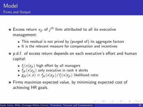
ModelFirms and Output

Excess return xjt of j th �rm attributed to all its executivemanagement:

This residual is not priced by (purged of) its aggregate factorsIt is the relevant measure for compensation and incentives

p.d.f. of excess return depends on each executive�s e¤ort and humancapital:

fj (x jzjt ) high e¤ort by all managersfjk (x jzjt ) only executive in rank k shirksgjk (x , z) � fjk (x jzjt )/fj (x jzjt ) likelihood ratio

Firms maximize expected value, by minimizing expected cost ofachieving HR goals.


36

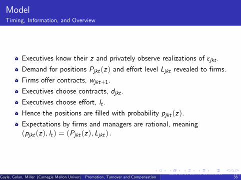
ModelTiming, Information, and Overview

Executives know their z and privately observe realizations of εjkt .

Demand for positions Pjkt (z) and e¤ort level Ljkt revealed to �rms.

Firms o¤er contracts, wjkt+1.

Executives choose contracts, djkt .

Executives choose e¤ort, lt .

Hence the positions are �lled with probability pjkt (z).

Expectations by �rms and managers are rational, meaning(pjkt (z), lt ) = (Pjkt (z), Ljkt ) .


36

Optimization by executivesOther assets held in smoothing over uncertain income sequences

Executives smooth their consumption over the winnings from playinga sequence of lotteries.

Let et denote the value of assets in t.

Let bt denote the bond price in t.

Let at denote the price of a security which pays a dividend of(λs lnλs � s ln β) each period where λs is the price of a consumptionunit in period s.

Those two assets are su¢ cient to achieve the optimal portfolio whenmarkets are complete.

See Rubinstein (1981) on aggregation.


36

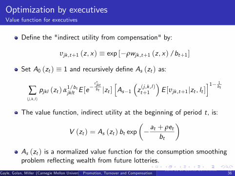
Optimization by executivesValue function for executives

De�ne the "indirect utility from compensation" by:

υjk ,t+1 (z , x) � exp [�ρwjk ,t+1 (z , x) /bt+1]

Set A0 (zt ) � 1 and recursively de�ne As (zt ) as:

∑(j ,k ,l)

pjkl (zt ) α1/btjklt E [e

�ε�jktbt jzt ]

hAs�1

�z (j ,k ,l)t+1

�E [υjk ,t+1jzt , lt ]

i1� 1bt

The value function, indirect utility at the beginning of period t, is:

V (zt ) = As (zt ) bt exp��at + ρet

bt

�As (zt ) is a normalized value function for the consumption smoothingproblem re�ecting wealth from future lotteries.


36

Optimization by executivesJob, �rm and e¤ort choice

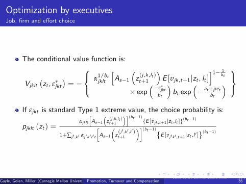
The conditional value function is:

Vjklt�zt , ε�jkt

�= �

8<: α1/btjklt

hAs�1

�z (j ,k ,lt )t+1

�E [υjk ,t+1jzt , lt ]

i1� 1bt

� exp��ε�jkt

bt

�bt exp

�� at+ρet

bt

�9=;

If εjkt is standard Type 1 extreme value, the choice probability is:

pjklt (zt ) =αjklt

hAs�1

�z (j ,k ,lt )t+1

�i(bt�1)fE [υjk ,t+1 jzt ,lt ]g(bt�1)1+∑j 0 ,k 0 αj 0k 0 l 0t

�As�1

�z(j 0 ,k 0 ,l 0)t+1

��(bt�1)fE [υj 0k 0 ,t+1 jzt ,l 0]g(bt�1)


36

Cost Minimizing ContractIncentive compatible contracts to correct moral hazard

If human capital is private information then the incentivecompatibility constraint is:

E [υjk ,t+1 (x) gjk (x , zt ) jzt ] ��

α1jktα0jk0t

� 1bt�1 A(j ,k ,1)s�1,t+1

A(j ,k ,0)s�1,t+1E [υjk ,t+1 (x) jzt ]

If human capital is public information, then the incentivecompatibility reduces to the standard moral hazard formulation:

E [υjk ,t+1 (x) g (x , zt ) jzt ] ��

α1jktα0jk0t

� 1bt�1

E [υjk ,t+1 (x) jzt ]

In the private information case, career concerns (may) help to o¤setcurrent bene�ts from shirking because human capital accumulationdepends on e¤ort, not just on participation.


36

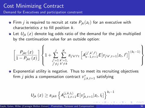
Cost Minimizing ContractDemand for Executives and participation constraint

Firm j is required to recruit at rate Pjk (zt ) for an executive withcharacteristics z to �ll position k.Let Ujk (z) denote log odds ratio of the demand for the job multipliedby the continuation value for an outside option:

�Pjkt (z)

1� Pjkt (z)

�8>><>>:1+J

∑j 0=1j 0 6=j

K

∑k 0=1,k 0 6=k

αj 0k 0 l 0t

hA(j

0,k 0,l 0)s�1,t+1E [υj 0k 0,t+1jzt , l 0]

i(bt�1)9>>=>>;

Exponential utility is negative. Thus to meet its recruiting objectives�rm j picks a compensation contract υ�j ,k ,t+1 satisfying

Ujk (z) � αjklt

nA(j ,k ,lt )s�1,t+1E [υ

�jk ,t+1jzt , lt ]

obt�1Gayle, Golan, Miller (Carnegie Mellon University)Promotion, Turnover and Compensation


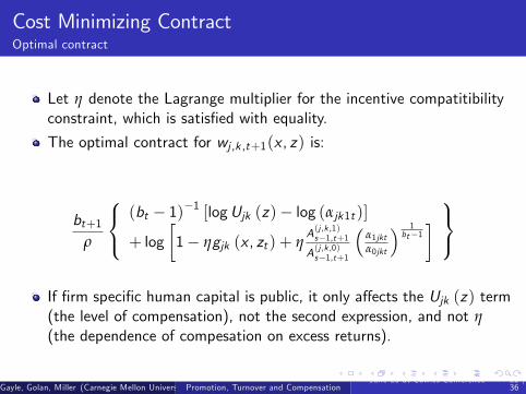
Cost Minimizing ContractOptimal contract

Let η denote the Lagrange multiplier for the incentive compatitibilityconstraint, which is satis�ed with equality.

The optimal contract for wj ,k ,t+1(x , z) is:

bt+1ρ

8<: (bt � 1)�1 [logUjk (z)� log (αjk1t )]

+ log�1� ηgjk (x , zt ) + η

A(j ,k ,1)s�1,t+1

A(j ,k ,0)s�1,t+1

�α1jktα0jkt

� 1bt�1

� 9=;If �rm speci�c human capital is public, it only a¤ects the Ujk (z) term(the level of compensation), not the second expression, and not η(the dependence of compesation on excess returns).


36

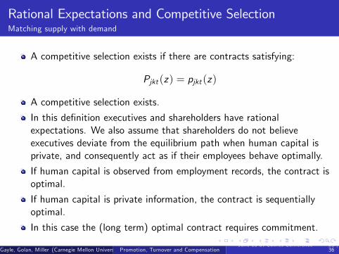
Rational Expectations and Competitive SelectionMatching supply with demand

A competitive selection exists if there are contracts satisfying:

Pjkt (z) = pjkt (z)

A competitive selection exists.

In this de�nition executives and shareholders have rationalexpectations. We also assume that shareholders do not believeexecutives deviate from the equilibrium path when human capital isprivate, and consequently act as if their employees behave optimally.

If human capital is observed from employment records, the contract isoptimal.

If human capital is private information, the contract is sequentiallyoptimal.

In this case the (long term) optimal contract requires commitment.


36

Identi�cation and EstimationData requirements

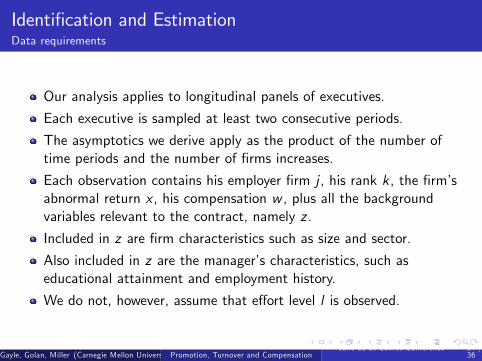
Our analysis applies to longitudinal panels of executives.

Each executive is sampled at least two consecutive periods.

The asymptotics we derive apply as the product of the number oftime periods and the number of �rms increases.

Each observation contains his employer �rm j , his rank k, the �rm�sabnormal return x , his compensation w , plus all the backgroundvariables relevant to the contract, namely z .

Included in z are �rm characteristics such as size and sector.

Also included in z are the manager�s characteristics, such aseducational attainment and employment history.

We do not, however, assume that e¤ort level l is observed.


36

Identi�cation and EstimationOverview

Estimation proceeds sequentially in six steps. Estimate:1 fj (x jz) nonparametrically from data on abnormal returns2 wojk (x , z) nonparametrically from data on compensation and abnormalreturns

3 Pjk (z) from data on executive choices4 ρ and α1jk (z) from market participation equation5 α0jk (z) from incentive compatibility condition6 gjk (x jz) from compensation equation

See Gayle and Miller (08): "Identifying and Testing . . . ".


36

Identi�cation and EstimationFourth step

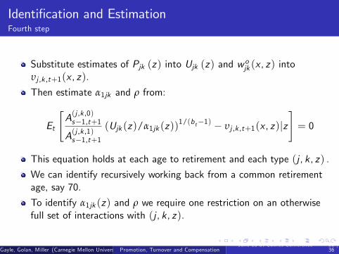
Substitute estimates of Pjk (z) into Ujk (z) and wojk (x , z) intoυj ,k ,t+1(x , z).

Then estimate α1jk and ρ from:

Et

"A(j ,k ,0)s�1,t+1

A(j ,k ,1)s�1,t+1(Ujk (z)/α1jk (z))

1/(bt�1) � υj ,k ,t+1(x , z)jz#= 0

This equation holds at each age to retirement and each type (j , k, z) .

We can identify recursively working back from a common retirementage, say 70.

To identify α1jk (z) and ρ we require one restriction on an otherwisefull set of interactions with (j , k, z).


36

Identi�cation and EstimationFifth step

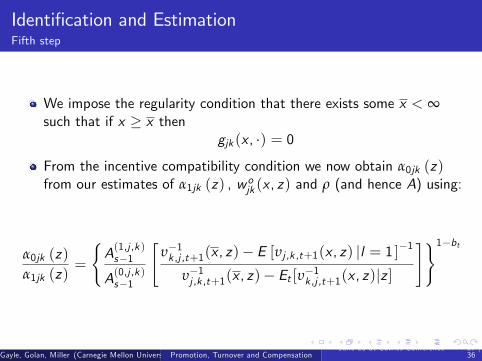
We impose the regularity condition that there exists some x < ∞such that if x � x then

gjk (x , �) = 0From the incentive compatibility condition we now obtain α0jk (z)from our estimates of α1jk (z) , wojk (x , z) and ρ (and hence A) using:

α0jk (z)α1jk (z)

=

(A(1,j ,k )s�1

A(0,j ,k )s�1

"υ�1k ,j ,t+1(x , z)� E [υj ,k ,t+1(x , z) jl = 1 ]

�1

υ�1j ,k ,t+1(x , z)� Et [υ�1k ,j ,t+1(x , z)jz ]

#)1�bt


36

Identi�cation and EstimationSixth step

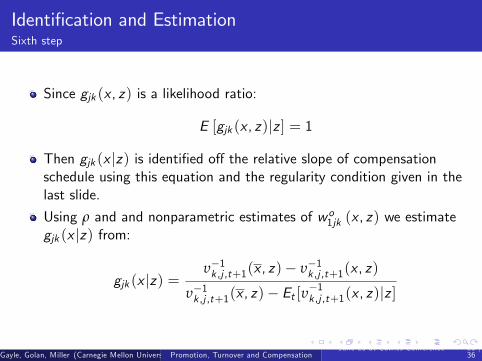
Since gjk (x , z) is a likelihood ratio:

E [gjk (x , z)jz ] = 1

Then gjk (x jz) is identi�ed o¤ the relative slope of compensationschedule using this equation and the regularity condition given in thelast slide.

Using ρ and and nonparametric estimates of wo1jk (x , z) we estimategjk (x jz) from:

gjk (x jz) =υ�1k ,j ,t+1(x , z)� υ�1k ,j ,t+1(x , z)

υ�1k ,j ,t+1(x , z)� Et [υ�1k ,j ,t+1(x , z)jz ]


36

Preliminary Empirical ResultsEstimated compensation schedule

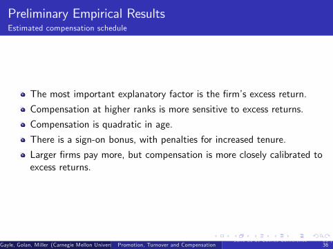
The most important explanatory factor is the �rm�s excess return.

Compensation at higher ranks is more sensitive to excess returns.

Compensation is quadratic in age.

There is a sign-on bonus, with penalties for increased tenure.

Larger �rms pay more, but compensation is more closely calibrated toexcess returns.


36

Preliminary Empirical ResultsSpan of control

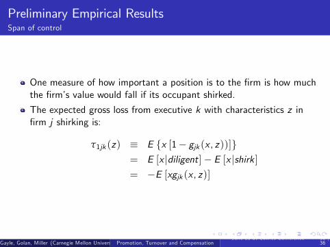
One measure of how important a position is to the �rm is how muchthe �rm�s value would fall if its occupant shirked.

The expected gross loss from executive k with characteristics z in�rm j shirking is:

τ1jk (z) � E fx [1� gjk (x , z))]g= E [x jdiligent]� E [x jshirk ]= �E [xgjk (x , z)]


36

Preliminary Empirical ResultsEstimated span of control and dispersion across �rms

τ1 is measured in percentage per yearMeasure Rank Estimates Standard Deviation.

ρ 0.45

τ1 1 5.2 3.42 10.9 143 8.3 2.94 4.2 2.75 1.6 1.2

The estimate of the risk aversion parameter implies a manager wouldpay up to $217,780 to insure himself against a fair bet of losingversus winning one million dollars.

Span of control is highest at rank 2, 11 percent per year.


36

Preliminary Empirical ResultsCompensating di¤erential for diligent work versus shirking

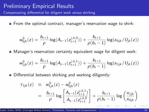
From the optimal contract, manager�s reservation wage to shirk:

w00jk (z) =bt+1

ρlog(As�1(z

j ,k ,0t+1 )) +

bt+1ρ(bt � 1)

log(α0jk/Ujk (z))

Manager�s reservation certainty equivalent wage for diligent work:

w01jk (z) =bt+1

ρlog(As�1(z

j ,k ,1t+1 )) +

bt+1ρ(bt � 1)

log(α1jk/Ujk (z))

Di¤erential between shirking and working diligently:

τ2jk (z) � w01jk (z)� w00jk (z)

=bt+1

ρlog

"As�1(z

j ,k ,1t+1 )

As�1(zj ,k ,0t+1

#+

bt+1ρ(bt � 1)

log�

α1jkα0jk

�Gayle, Golan, Miller (Carnegie Mellon University)Promotion, Turnover and Compensation


Preliminary Empirical ResultsHow career concerns alleviate moral hazard

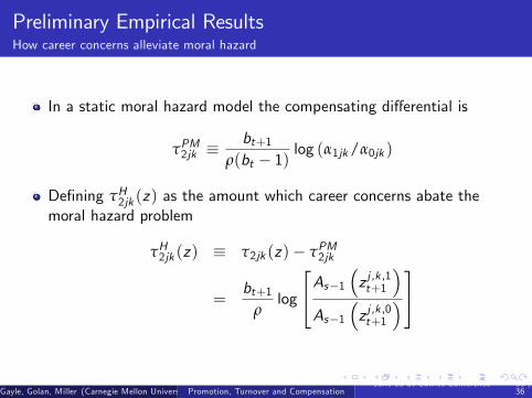
In a static moral hazard model the compensating di¤erential is

τPM2jk �bt+1

ρ(bt � 1)log (α1jk/α0jk )

De�ning τH2jk (z) as the amount which career concerns abate themoral hazard problem

τH2jk (z) � τ2jk (z)� τPM2jk

=bt+1

ρlog

24As�1�z j ,k ,1t+1

�As�1

�z j ,k ,0t+1

�35


36

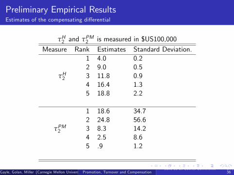
Preliminary Empirical ResultsEstimates of the compensating di¤erential

τH2 and τPM2 is measured in $US100,000

Measure Rank Estimates Standard Deviation.1 4.0 0.22 9.0 0.5

τH2 3 11.8 0.94 16.4 1.35 18.8 2.2

1 18.6 34.72 24.8 56.6

τPM2 3 8.3 14.24 2.5 8.65 .9 1.2


36

Preliminary Empirical ResultsThe welfare cost of moral hazard

Firms pay the di¤erence between expected compensation and itscertainty equivalent to resolve moral hazard:

τ3jk = E [wjk (x) jz ]� w01jk (z)

= E [wjk (x) jz ]�bt+1

ρlog(As�1(z

j ,k ,1t+1 ))

� bt+1ρ(bt � 1)

log [α1jk/Ujk (z)]

If there were no career concerns, the additional cost of moral hazardto the �rm would be

τ4jk (z) �bt+1

ρlog(As�1(z

j ,k ,1t+1 ))


36

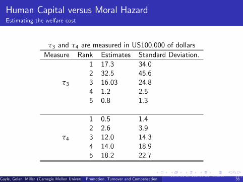
Human Capital versus Moral HazardEstimating the welfare cost

τ3 and τ4 are measured in US100,000 of dollarsMeasure Rank Estimates Standard Deviation.

1 17.3 34.02 32.5 45.6

τ3 3 16.03 24.84 1.2 2.55 0.8 1.3

1 0.5 1.42 2.6 3.9

τ4 3 12.0 14.34 14.0 18.95 18.2 22.7


36

Documents

Promotion, Turnover and Compensation in the Executive Market · · 2015-07-14Promotion, Turnover and Compensation in the Executive Market ... Miller (Carnegie Mellon University)Promotion,