Projection onto the Manifold of Elongated

Structures for Accurate Extraction

Amos Sironi1∗ Vincent Lepetit1,2 Pascal Fua1

1CVLab, EPFL, Lausanne, Switzerland, {firstname.lastname}@epfl.ch2TU Graz, Graz, Austria, lepetit@icg.tugraz.at

Abstract

Detection of elongated structures in 2D images and 3D

image stacks is a critical prerequisite in many applica-

tions and Machine Learning-based approaches have re-

cently been shown to deliver superior performance. How-

ever, these methods essentially classify individual locations

and do not explicitly model the strong relationship that ex-

ists between neighboring ones. As a result, isolated erro-

neous responses, discontinuities, and topological errors are

present in the resulting score maps.

We solve this problem by projecting patches of the score

map to their nearest neighbors in a set of ground truth train-

ing patches. Our algorithm induces global spatial consis-

tency on the classifier score map and returns results that are

provably geometrically consistent. We apply our algorithm

to challenging datasets in four different domains and show

that it compares favorably to state-of-the-art methods.

1. Introduction

Reliably extracting boundaries from images is a long-

standing open Computer Vision problem and finding 3D

membranes, their equivalent in biomedical image stacks,

while difficult is often a prerequisite to their segmentation.

Similarly in both regular images and image stacks, recon-

structing the centerline of linear structures is a critical first

step in many applications, ranging from road delineation in

2D aerial images to modeling neurites and blood vessels in

3D biomedical image stacks.

These problems are all similar in that they involve find-

ing elongated structures of codimension 1 or 2 given very

noisy data. In all these cases, classification- and regression-

based approaches [9, 38, 39] have recently proved to yield

better performance than those that rely on hand-designed

filters. This success is attributable to the representations

used by powerful machine learning techniques [23, 43] op-

erating on large training datasets.

However, these methods essentially classify individual

∗This work was supported in part by the EU ERC project MicroNano.

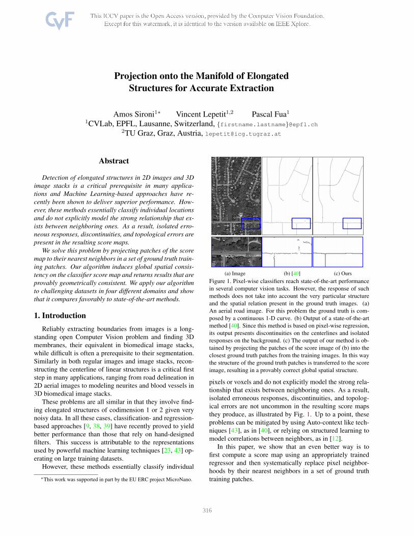
(a) Image (b) [40] (c) Ours

Figure 1. Pixel-wise classifiers reach state-of-the-art performance

in several computer vision tasks. However, the response of such

methods does not take into account the very particular structure

and the spatial relation present in the ground truth images. (a)

An aerial road image. For this problem the ground truth is com-

posed by a continuous 1-D curve. (b) Output of a state-of-the-art

method [40]. Since this method is based on pixel-wise regression,

its output presents discontinuities on the centerlines and isolated

responses on the background. (c) The output of our method is ob-

tained by projecting the patches of the score image of (b) into the

closest ground truth patches from the training images. In this way

the structure of the ground truth patches is transferred to the score

image, resulting in a provably correct global spatial structure.

pixels or voxels and do not explicitly model the strong rela-

tionship that exists between neighboring ones. As a result,

isolated erroneous responses, discontinuities, and topolog-

ical errors are not uncommon in the resulting score maps

they produce, as illustrated by Fig. 1. Up to a point, these

problems can be mitigated by using Auto-context like tech-

niques [43], as in [40], or relying on structured learning to

model correlations between neighbors, as in [12].

In this paper, we show that an even better way is to

first compute a score map using an appropriately trained

regressor and then systematically replace pixel neighbor-

hoods by their nearest neighbors in a set of ground truth

training patches.

316

This is in the spirit of algorithms for image denoising

and inpainting that search for nearest neighbors within the

image itself [11, 10, 25]. It is also closely related to the

approach of [16] that improves boundary images by finding

nearest neighbors using a distance defined in terms of de-

scriptors extracted by a Convolutional Neural Network. By

contrast, in our method, we compute distances in terms of

the patches themselves and we will show that it improves

both performance, especially near junctions, and generality.

In short, our algorithm induces global spatial consistency

on the classifier score map and improves classification per-

formance, as can be seen in Fig. 1(c). Furthermore, assum-

ing that the structure of all admissible ground truth images

is well represented by the set of training patches, it can be

formally shown that our method is equivalent to projecting

the score map into the manifold of all admissible ground

truth maps.

2. Related Work

In this section, we review related work on centerline,

boundary and membrane detection.

Centerline Detection Centerline detection methods can

be divided in two main classes.

The first class relies on hand-designed filters. They are

typically used to compute the Hessian matrix [14, 36, 28,

13, 29] or the Oriented Flux matrix [22, 1, 41, 33, 44],

whose eigenvalues then serve to estimate the likelihood that

a pixel or voxel lies on a centerline. Since the filters are

optimized for ideal tubular structure, their performance de-

creases when the structures of interest become irregular.

To overcome this limitation, a second class of meth-

ods that rely on Machine Learning techniques has recently

emerged. Classification-based ones [17, 47, 7, 46] have

been successfully applied to the segmentation of thick lin-

ear structures while, regression-based ones [39, 40] have

been shown to be particularly effective at finding centerline

pixels only. However, even if pixel-wise classification and

regression methods can produce remarkable results, they do

not explicitly model the strong relationship that exists be-

tween neighboring pixels. As a consequence, discontinu-

ities and inconsistencies may occur in their output.

Boundary Detection Boundary detection methods can be

divided in the same two classes as for centerline detection.

All the early approaches [26, 8, 32] belong to the first

one and rely on filters designed to respond to specific image

intensity profiles. Recently, attention has shifted to classi-

fication based methods [5, 34, 38, 24, 12], which have pro-

duced significant improvements.

More specifically, in [5] gradients on different image

channels are fed to a logistic regression classifier to predict

contours. In [34], SVMs are trained to predict boundaries

from features computed using sparse coding. In [9], a Deep

Convolutional Network is used to segment cell membranes

in 2D Electron Microscopy slices, while a sequence of clas-

sifiers is used in [38] for boundary detection in both natural

images and Electron Microscopy data.

However, as in the case of centerline detection, none

of these methods explicitly model the relationship between

nearby pixels. In particular, the response of Convolutional

Neural Networks [23] can be spatially inconsistent because

they typically treat every pixel location independently, thus

relying only on the fact that neighboring patches share pix-

els to enforce consistency.

By contrast, in Auto-context based methods [43, 38],

features extracted from the classifiers output in earlier lay-

ers enlarge the receptive field and often yield more spatially

consistence results. However, these methods are prone to

overfitting and require large amount of training data to pre-

vent it. The method of [12] overcomes these problems by

relying on structured learning, resulting in an accurate and

extremely efficient edge detector. It is inspired by the work

of [20, 21] where the structured random forest framework is

introduced for image labeling purposes, predicting for every

pixel an image patch, instead of single pixel probabilities.

However, it is specific to the particular kind of classifier

used for learning and is difficult to generalize.

Recently, Nearest Neighbors search in the space of lo-

cal descriptors obtained with a Convolutional Network was

used for boundary detection purposes [16]. Given an im-

age patch, the algorithm computes a corresponding descrip-

tor and then looks for the Nearest Neighbor in a dictionary

built from the training set. While effective, this approach

strongly depends on the specific dictionary learned by the

CNN. Therefore, when it fails, it is difficult to understand

why. Our method is closely related, but we perform Nearest

Neighbors search in the space of the final output, rather than

of intermediate image features. We will show empirically

that it works better, especially near junctions. Moreover,

unlike other approaches, ours is provably correct under cer-

tain conditions, thus giving insights and indications on how

to improve the results.

Membrane Detection Membranes are the 3D equiva-

lent of contours in image stacks. They are important for

3D volume segmentation, especially in a biomedical con-

text [45, 4, 15]. In the previous paragraph we mentioned

algorithms [9, 38] that extract them 2D slice by 2D slice.

Here we discuss those that extract them as 3D surfaces.

As in the case of 2D boundaries, early approaches to de-

tecting them relied on hand-crafted filters optimized to re-

spond to ideal sheet-like structures. In [37, 30, 27] for ex-

ample, the eigenvalues of the Hessian matrix are combined

to obtain a score value that is maximal for voxels lying on a

2D surface. Similarly, the eigenvalues of the Oriented Flux

matrix [22] can be combined to obtain a score that is less

sensitive to adjacent structures.

317

More recent approaches have focused on machine learn-

ing techniques. For example, a Convolutional Neural

Network and a hierarchical segmentation framework com-

bining Random Forest classifier and watersheds are used

in [19] and [3] respectively to segment neural membranes.

Even though both of these methods produce excellent re-

sults, they are designed for tissue samples prepared with an

extra-cellular die that highlights cell membranes while sup-

pressing the intracellular structures, thus making the task

comparatively easy.

3. Motivation and Formalization

As discussed in Section 2, methods that rely on statistical

classification techniques currently deliver the best results

for boundary, centerline, and membrane detection. Among

those, it has recently been reported that regression-based

ones perform best for centerline detection [39] and we will

demonstrate here that they perform equally well for bound-

ary and membrane detection.

More specifically, the algorithm of [39] involves train-

ing regressors to return distances to the closest centerline

in scale-space. In this way, performing non-maximum sup-

pression on their output yields both centerline locations and

corresponding scales. This has proved very effective but,

like for all other pixel-based techniques that do not incor-

porate any a priori geometric knowledge that may be avail-

able, this approach can easily result in topological mistakes.

In this paper, we first extend this approach to both bound-

ary and membrane detection. We then demonstrate that we

can correct the errors it makes by projecting them into the

manifold of distance transforms corresponding to the kind

of structures we are trying to reconstruct. This results in a

technique that is both a more competent and more widely

applicable method than the original one [39]. Furthermore,

it is generic in the sense that it is applicable to other meth-

ods returning a score map, such as [12, 9].

In the remainder of this section, we first summarize

the approach of [39] and show that it extends naturally to

boundary and membrane detection. We also introduce the

formalism that we will use in the next section to describe

our approach to improving the distance transforms by pro-

jecting them onto an appropriate manifold.

3.1. Centerline Detection

Let I ∈ RN be an image containing linear structures and

let Y be the corresponding binary ground truth image, such

that Y (p) = 1 if pixel p is on a centerline and Y (p) = 0otherwise.

Finding the centerlines can be formulated as the pixel

classification problem of learning a mapping between a fea-

ture vector fM (p, I), extracted from a local neighborhood

NM (p) of size M around pixel p in image I , and the value

Y (p).

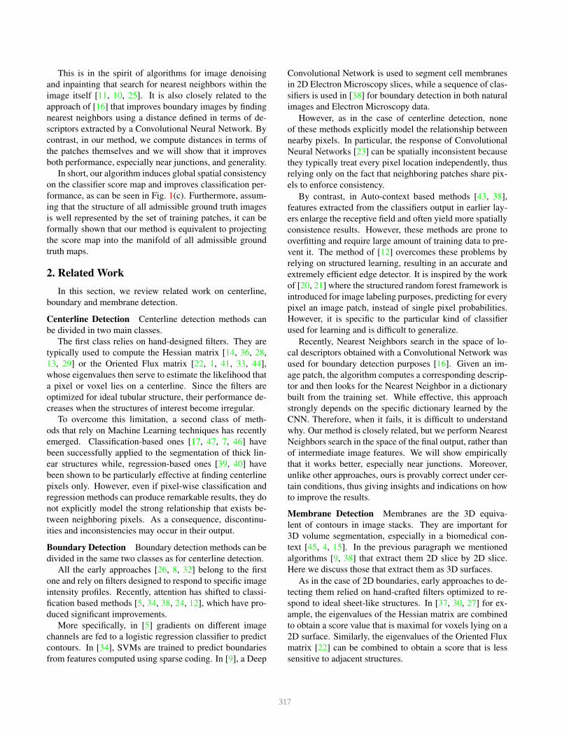
(a) (b) (c) (d) (e)

Figure 2. Centerline Detection as a Regression Problem. (a) Origi-

nal image patch; (b) Centerlines Ground Truth; (c) Distance Func-

tion of Eq. (1) proposed in [39]; (d) The response of a pixel-

wise regressor trained to predict the function in (c) is discontin-

uous and returns topologically incorrect results, also when Auto-

context [43] is applied. (e) Nearest Neighbors of the score patches

in (d), found in the training set. In our method we apply Nearest

Neighbors search to a regressor output and take advantage of the

particular structure of ground truth patches to correct its mistakes.

Learning such a classifier, however, can be difficult in

practice because of the similar aspect of nearby pixels to the

centerline and ambiguities on the exact location of a center-

line due to low resolution and blurring.

To address this difficulty, the method of [39] replaces the

binary ground truth Y by the modified distance transform

of Y

d(p) =

{

ea(1−

DY (p)dM

)− 1 if DY (p) < dM

0 otherwise, (1)

where DY is the Euclidean distance transform of Y , a > 0is a constant that controls the exponential decrease rate of d

close to the centerline and dM a threshold value determining

how far from a centerline d is set to zero.

Function d has a sharp maximum along the center-

lines and decreases as one moves further from them.

Fig. 2(c) shows examples of function d computed on small

patches. Learning a regressor to associate the feature vector

fM (p, I) to d(p) induces a unique local maximum in the

neighborhood of the centerlines. This approach is more ro-

bust to small displacements and returns centerlines that are

better localized compared to classification-based methods.

To learn the regressor we apply the GradientBoost al-

gorithm [18]. Given training data {fi, di}i, where fi =fM (pi, I) is the feature vector corresponding to pixel piand di = d(pi), GradientBoost learns a function ϕ(·) of

the form ϕ(q) =∑T

t=1αtht(q) , where q = fM (p, I) de-

notes a feature vector, ht are weak learners and αt ∈ R are

weights. Function ϕ is built iteratively, selecting one weak

learner and its weight at each iteration, to minimize a loss

function L of the form L =∑

i L(di, ϕ(fi)).

318

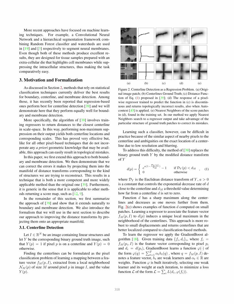
Input Image I Regressor Score Map X Output ΠD N(X)

Nearest Neighbor

xi

Centerlines

... ...}

}Train Gt Patches

NMSΠ(xi)

φ

Figure 3. Method overview. A score map X is obtained from image I by applying a regressor ϕ trained to return distances from the

centerlines. Every patch xi of size D in X is projected onto the set of ground truth training patches, by nearest neigbor search. The

projected patches ΠN (xi) are averaged to form the output score map ΠD→N (X). Centerlines are obtained by Non-Maxima Suppression.

In addition, to learn the best possible regressor, we

adopted the Auto-context technique [43], as in [40] and us-

ing the same parameters. To this end, we use the score map

ϕ(·) to extract a new set of features that are added to the

original ones to train a new regressor.

3.2. Boundary and Membrane Detection

The method described above extends naturally to bound-

ary detection. As centerlines, boundary in 2D images and

membranes in 3D image stacks are elongated structures of

codimension 1 and there are substantial ambiguities in the

exact boundary location.

Therefore, and as before, we replace the binary ground

truth, provided for such problems, by the distance transform

of Eq. (1). The distance function is computed 2D for bound-

aries and 3D for membranes. We then train a regressor to

associate feature vectors to the distances to the boundaries.

We can obtain the boundaries from the score map returned

by the regressor by non-maxima suppression.

4. Improving the Distance Function

The central element of our approach is to project the dis-

tance transform produced by pixel-wise regression, as de-

scribed in the previous section, onto the manifold of all pos-

sible ones for the structures of interest. Since this manifold

is much too large to be computed in practice, we first pro-

pose a practical computational scheme and then formally

prove that it provides a close approximation under assump-

tions that can be made to hold in the real world.

4.1. Nearest Neighbors Projections

Given an image I and corresponding binary ground truth

Y , let dY be the image obtained by applying function d of

Eq. (1) to every pixel of Y . Since it corresponds to pixels

belonging to specific structures, Y is constrained to have

well defined geometric properties. For example, in the case

of centerlines or boundaries in images, Y is composed of

1-dimensional curves, while for boundaries in 3D volumes,

Y is a 2D surface. This means that the set of all admissible

ground truths forms a manifold in the set of binary images.

Similarly, the set of images dY forms a manifold in the set

of real valued images, which we will denote by MN .

Let X be the score map obtained by applying the regres-

sor ϕ to each pixel of an input image I . Ideally we would

like X to be an element of MN , so that it is guaranteed to be

geometrically correct. However, this is not true in general.

Fig. 2(d) shows typical errors committed at critical points,

such as T-junctions. This is a standard problem with many

edge detectors, such as the Canny detector.

In theory, one way to avoid this problem is to project

X into MN , which is equivalent to finding the element of

MN closest to X ,

ΠN (X) = argmindY ∈MN

‖dY −X‖2. (2)

In practice, however, MN is not known or much too large

to be sampled exhaustively. Therefore, ΠN (X) can not be

computed directly.

As shown in Fig. 3, our solution is to approximate it by

projecting small patches of X onto the set of ground truth

train patches.

Formally, let MD = {yk}Kk=1

be the set of training

patches of size D, extracted form local neighborhoods ND

in the ground truth training images. For each pixel pi,

i = 1, . . . , N in the score image X , let xi = X(ND(pi))be the squared neighborhood of size D around pi.

For every i, we consider the projection of xi into MD,

given by

ΠD(xi) = argminy∈MD

‖y − xi‖2. (3)

Fig. 2(d) shows examples of nearest neighbors for three

score patches. We then average all these projections to ob-

tain a new score image ΠD→N (X).

319

X xi

ΠD N

ΠD

ΠN

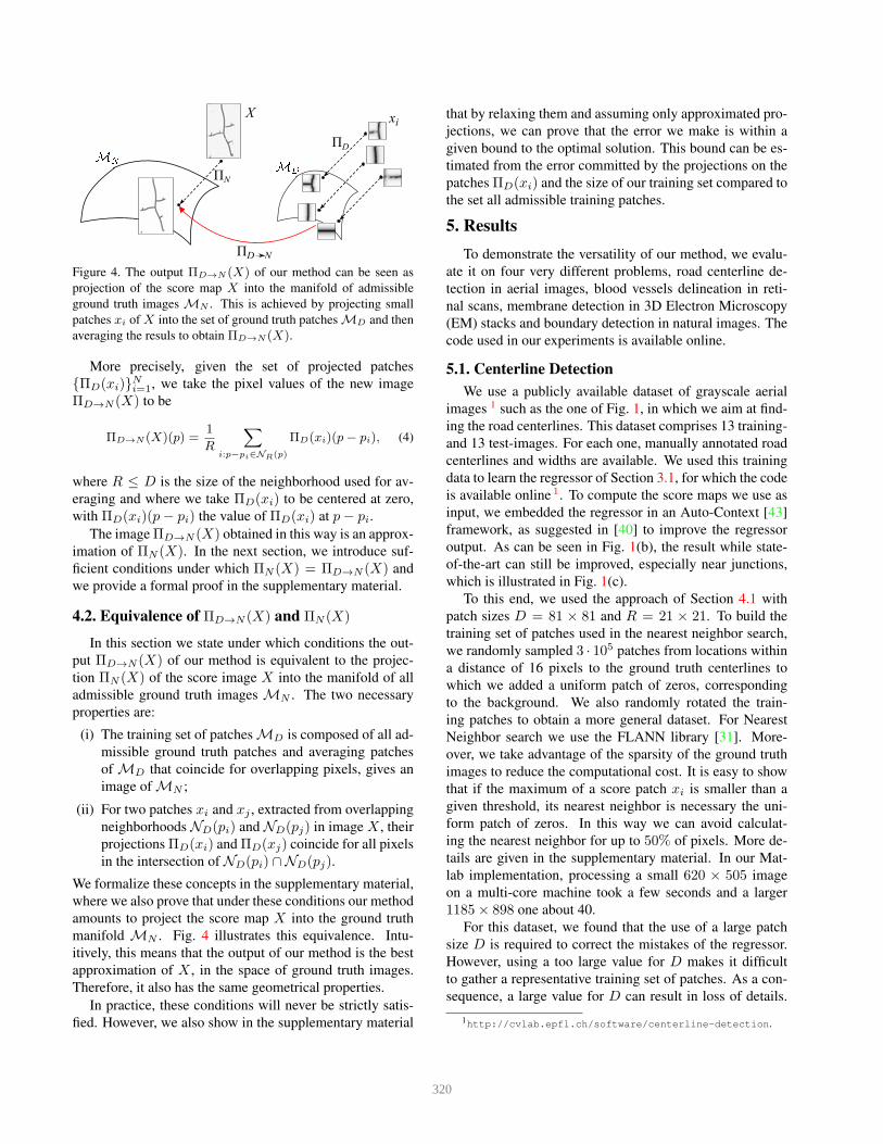
Figure 4. The output ΠD→N (X) of our method can be seen as

projection of the score map X into the manifold of admissible

ground truth images MN . This is achieved by projecting small

patches xi of X into the set of ground truth patches MD and then

averaging the resuls to obtain ΠD→N (X).

More precisely, given the set of projected patches

{ΠD(xi)}Ni=1

, we take the pixel values of the new image

ΠD→N (X) to be

ΠD→N (X)(p) =1

R

∑

i:p−pi∈NR(p)

ΠD(xi)(p− pi), (4)

where R ≤ D is the size of the neighborhood used for av-

eraging and where we take ΠD(xi) to be centered at zero,

with ΠD(xi)(p− pi) the value of ΠD(xi) at p− pi.

The image ΠD→N (X) obtained in this way is an approx-

imation of ΠN (X). In the next section, we introduce suf-

ficient conditions under which ΠN (X) = ΠD→N (X) and

we provide a formal proof in the supplementary material.

4.2. Equivalence of ΠD→N (X) and ΠN (X)

In this section we state under which conditions the out-

put ΠD→N (X) of our method is equivalent to the projec-

tion ΠN (X) of the score image X into the manifold of all

admissible ground truth images MN . The two necessary

properties are:

(i) The training set of patches MD is composed of all ad-

missible ground truth patches and averaging patches

of MD that coincide for overlapping pixels, gives an

image of MN ;

(ii) For two patches xi and xj , extracted from overlapping

neighborhoods ND(pi) and ND(pj) in image X , their

projections ΠD(xi) and ΠD(xj) coincide for all pixels

in the intersection of ND(pi) ∩ND(pj).

We formalize these concepts in the supplementary material,

where we also prove that under these conditions our method

amounts to project the score map X into the ground truth

manifold MN . Fig. 4 illustrates this equivalence. Intu-

itively, this means that the output of our method is the best

approximation of X , in the space of ground truth images.

Therefore, it also has the same geometrical properties.

In practice, these conditions will never be strictly satis-

fied. However, we also show in the supplementary material

that by relaxing them and assuming only approximated pro-

jections, we can prove that the error we make is within a

given bound to the optimal solution. This bound can be es-

timated from the error committed by the projections on the

patches ΠD(xi) and the size of our training set compared to

the set all admissible training patches.

5. Results

To demonstrate the versatility of our method, we evalu-

ate it on four very different problems, road centerline de-

tection in aerial images, blood vessels delineation in reti-

nal scans, membrane detection in 3D Electron Microscopy

(EM) stacks and boundary detection in natural images. The

code used in our experiments is available online.

5.1. Centerline Detection

We use a publicly available dataset of grayscale aerial

images 1 such as the one of Fig. 1, in which we aim at find-

ing the road centerlines. This dataset comprises 13 training-

and 13 test-images. For each one, manually annotated road

centerlines and widths are available. We used this training

data to learn the regressor of Section 3.1, for which the code

is available online 1. To compute the score maps we use as

input, we embedded the regressor in an Auto-Context [43]

framework, as suggested in [40] to improve the regressor

output. As can be seen in Fig. 1(b), the result while state-

of-the-art can still be improved, especially near junctions,

which is illustrated in Fig. 1(c).

To this end, we used the approach of Section 4.1 with

patch sizes D = 81 × 81 and R = 21 × 21. To build the

training set of patches used in the nearest neighbor search,

we randomly sampled 3 · 105 patches from locations within

a distance of 16 pixels to the ground truth centerlines to

which we added a uniform patch of zeros, corresponding

to the background. We also randomly rotated the train-

ing patches to obtain a more general dataset. For Nearest

Neighbor search we use the FLANN library [31]. More-

over, we take advantage of the sparsity of the ground truth

images to reduce the computational cost. It is easy to show

that if the maximum of a score patch xi is smaller than a

given threshold, its nearest neighbor is necessary the uni-

form patch of zeros. In this way we can avoid calculat-

ing the nearest neighbor for up to 50% of pixels. More de-

tails are given in the supplementary material. In our Mat-

lab implementation, processing a small 620 × 505 image

on a multi-core machine took a few seconds and a larger

1185× 898 one about 40.

For this dataset, we found that the use of a large patch

size D is required to correct the mistakes of the regressor.

However, using a too large value for D makes it difficult

to gather a representative training set of patches. As a con-

sequence, a large value for D can result in loss of details.

1http://cvlab.epfl.ch/software/centerline-detection.

320

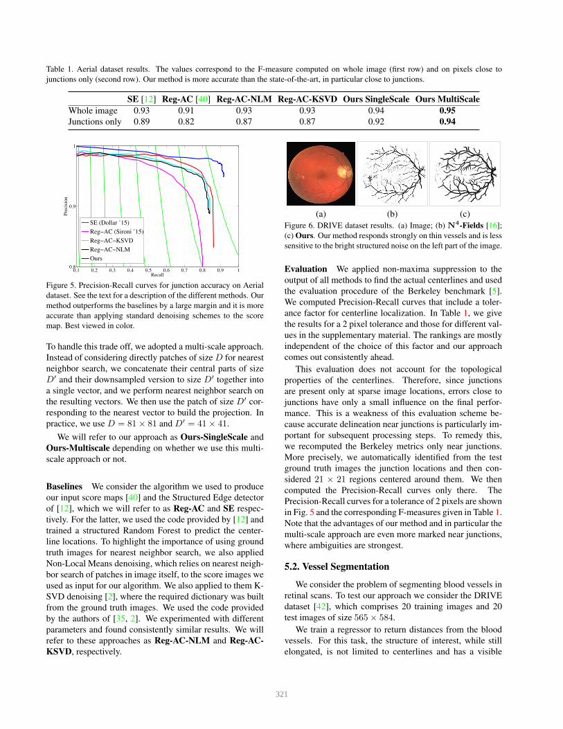
Table 1. Aerial dataset results. The values correspond to the F-measure computed on whole image (first row) and on pixels close to

junctions only (second row). Our method is more accurate than the state-of-the-art, in particular close to junctions.

SE [12] Reg-AC [40] Reg-AC-NLM Reg-AC-KSVD Ours SingleScale Ours MultiScale

Whole image 0.93 0.91 0.93 0.93 0.94 0.95

Junctions only 0.89 0.82 0.87 0.87 0.92 0.94

0.1 0.2 0.3 0.4 0.5 0.6 0.7 0.8 0.9 10.8

0.9

1

Recall

Pre

cisi

on

SE (Dollar ’15)

Reg AC (Sironi ’15)

Reg AC KSVD

Reg AC NLM

Ours

Figure 5. Precision-Recall curves for junction accuracy on Aerial

dataset. See the text for a description of the different methods. Our

method outperforms the baselines by a large margin and it is more

accurate than applying standard denoising schemes to the score

map. Best viewed in color.

To handle this trade off, we adopted a multi-scale approach.

Instead of considering directly patches of size D for nearest

neighbor search, we concatenate their central parts of size

D′ and their downsampled version to size D′ together into

a single vector, and we perform nearest neighbor search on

the resulting vectors. We then use the patch of size D′ cor-

responding to the nearest vector to build the projection. In

practice, we use D = 81× 81 and D′ = 41× 41.

We will refer to our approach as Ours-SingleScale and

Ours-Multiscale depending on whether we use this multi-

scale approach or not.

Baselines We consider the algorithm we used to produce

our input score maps [40] and the Structured Edge detector

of [12], which we will refer to as Reg-AC and SE respec-

tively. For the latter, we used the code provided by [12] and

trained a structured Random Forest to predict the center-

line locations. To highlight the importance of using ground

truth images for nearest neighbor search, we also applied

Non-Local Means denoising, which relies on nearest neigh-

bor search of patches in image itself, to the score images we

used as input for our algorithm. We also applied to them K-

SVD denoising [2], where the required dictionary was built

from the ground truth images. We used the code provided

by the authors of [35, 2]. We experimented with different

parameters and found consistently similar results. We will

refer to these approaches as Reg-AC-NLM and Reg-AC-

KSVD, respectively.

(a) (b) (c)

Figure 6. DRIVE dataset results. (a) Image; (b) N4-Fields [16];

(c) Ours. Our method responds strongly on thin vessels and is less

sensitive to the bright structured noise on the left part of the image.

Evaluation We applied non-maxima suppression to the

output of all methods to find the actual centerlines and used

the evaluation procedure of the Berkeley benchmark [5].

We computed Precision-Recall curves that include a toler-

ance factor for centerline localization. In Table 1, we give

the results for a 2 pixel tolerance and those for different val-

ues in the supplementary material. The rankings are mostly

independent of the choice of this factor and our approach

comes out consistently ahead.

This evaluation does not account for the topological

properties of the centerlines. Therefore, since junctions

are present only at sparse image locations, errors close to

junctions have only a small influence on the final perfor-

mance. This is a weakness of this evaluation scheme be-

cause accurate delineation near junctions is particularly im-

portant for subsequent processing steps. To remedy this,

we recomputed the Berkeley metrics only near junctions.

More precisely, we automatically identified from the test

ground truth images the junction locations and then con-

sidered 21 × 21 regions centered around them. We then

computed the Precision-Recall curves only there. The

Precision-Recall curves for a tolerance of 2 pixels are shown

in Fig. 5 and the corresponding F-measures given in Table 1.

Note that the advantages of our method and in particular the

multi-scale approach are even more marked near junctions,

where ambiguities are strongest.

5.2. Vessel Segmentation

We consider the problem of segmenting blood vessels in

retinal scans. To test our approach we consider the DRIVE

dataset [42], which comprises 20 training images and 20

test images of size 565× 584.

We train a regressor to return distances from the blood

vessels. For this task, the structure of interest, while still

elongated, is not limited to centerlines and has a visible

321

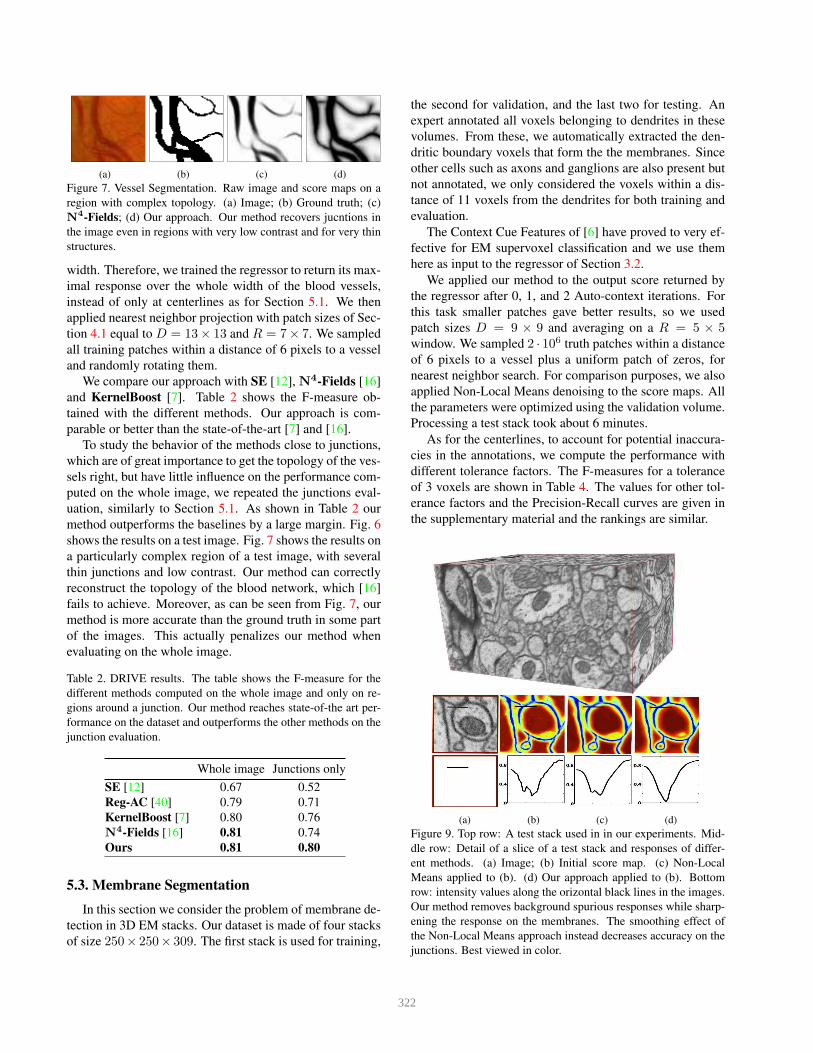
(a) (b) (c) (d)

Figure 7. Vessel Segmentation. Raw image and score maps on a

region with complex topology. (a) Image; (b) Ground truth; (c)

N4-Fields; (d) Our approach. Our method recovers jucntions in

the image even in regions with very low contrast and for very thin

structures.

width. Therefore, we trained the regressor to return its max-

imal response over the whole width of the blood vessels,

instead of only at centerlines as for Section 5.1. We then

applied nearest neighbor projection with patch sizes of Sec-

tion 4.1 equal to D = 13× 13 and R = 7× 7. We sampled

all training patches within a distance of 6 pixels to a vessel

and randomly rotating them.

We compare our approach with SE [12], N4-Fields [16]

and KernelBoost [7]. Table 2 shows the F-measure ob-

tained with the different methods. Our approach is com-

parable or better than the state-of-the-art [7] and [16].

To study the behavior of the methods close to junctions,

which are of great importance to get the topology of the ves-

sels right, but have little influence on the performance com-

puted on the whole image, we repeated the junctions eval-

uation, similarly to Section 5.1. As shown in Table 2 our

method outperforms the baselines by a large margin. Fig. 6

shows the results on a test image. Fig. 7 shows the results on

a particularly complex region of a test image, with several

thin junctions and low contrast. Our method can correctly

reconstruct the topology of the blood network, which [16]

fails to achieve. Moreover, as can be seen from Fig. 7, our

method is more accurate than the ground truth in some part

of the images. This actually penalizes our method when

evaluating on the whole image.

Table 2. DRIVE results. The table shows the F-measure for the

different methods computed on the whole image and only on re-

gions around a junction. Our method reaches state-of-the art per-

formance on the dataset and outperforms the other methods on the

junction evaluation.

Whole image Junctions only

SE [12] 0.67 0.52

Reg-AC [40] 0.79 0.71

KernelBoost [7] 0.80 0.76

N4-Fields [16] 0.81 0.74

Ours 0.81 0.80

5.3. Membrane Segmentation

In this section we consider the problem of membrane de-

tection in 3D EM stacks. Our dataset is made of four stacks

of size 250× 250× 309. The first stack is used for training,

the second for validation, and the last two for testing. An

expert annotated all voxels belonging to dendrites in these

volumes. From these, we automatically extracted the den-

dritic boundary voxels that form the the membranes. Since

other cells such as axons and ganglions are also present but

not annotated, we only considered the voxels within a dis-

tance of 11 voxels from the dendrites for both training and

evaluation.

The Context Cue Features of [6] have proved to very ef-

fective for EM supervoxel classification and we use them

here as input to the regressor of Section 3.2.

We applied our method to the output score returned by

the regressor after 0, 1, and 2 Auto-context iterations. For

this task smaller patches gave better results, so we used

patch sizes D = 9 × 9 and averaging on a R = 5 × 5window. We sampled 2 · 106 truth patches within a distance

of 6 pixels to a vessel plus a uniform patch of zeros, for

nearest neighbor search. For comparison purposes, we also

applied Non-Local Means denoising to the score maps. All

the parameters were optimized using the validation volume.

Processing a test stack took about 6 minutes.

As for the centerlines, to account for potential inaccura-

cies in the annotations, we compute the performance with

different tolerance factors. The F-measures for a tolerance

of 3 voxels are shown in Table 4. The values for other tol-

erance factors and the Precision-Recall curves are given in

the supplementary material and the rankings are similar.

(a) (b) (c) (d)

Figure 9. Top row: A test stack used in in our experiments. Mid-

dle row: Detail of a slice of a test stack and responses of differ-

ent methods. (a) Image; (b) Initial score map. (c) Non-Local

Means applied to (b). (d) Our approach applied to (b). Bottom

row: intensity values along the orizontal black lines in the images.

Our method removes background spurious responses while sharp-

ening the response on the membranes. The smoothing effect of

the Non-Local Means approach instead decreases accuracy on the

junctions. Best viewed in color.

322

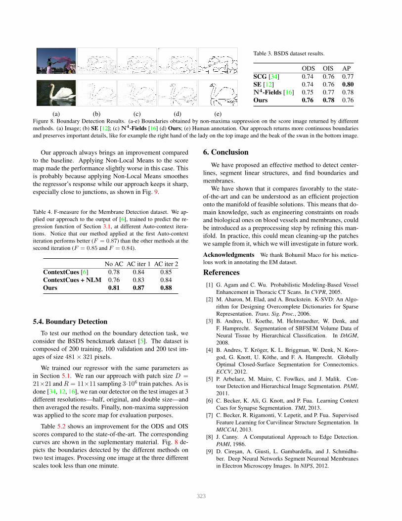
(a) (b) (c) (d) (e)

Table 3. BSDS dataset results.

ODS OIS AP

SCG [34] 0.74 0.76 0.77

SE [12] 0.74 0.76 0.80

N4-Fields [16] 0.75 0.77 0.78

Ours 0.76 0.78 0.76

Figure 8. Boundary Detection Results. (a-e) Boundaries obtained by non-maxima suppression on the score image returned by different

methods. (a) Image; (b) SE [12]; (c) N4-Fields [16] (d) Ours; (e) Human annotation. Our approach returns more continuous boundaries

and preserves important details, like for example the right hand of the lady on the top image and the beak of the swan in the bottom image.

Our approach always brings an improvement compared

to the baseline. Applying Non-Local Means to the score

map made the performance slightly worse in this case. This

is probably because applying Non-Local Means smoothes

the regressor’s response while our approach keeps it sharp,

especially close to junctions, as shown in Fig. 9.

Table 4. F-measure for the Membrane Detection dataset. We ap-

plied our approach to the output of [6], trained to predict the re-

gression function of Section 3.1, at different Auto-context itera-

tions. Notice that our method applied at the first Auto-context

iteration performs better (F = 0.87) than the other methods at the

second iteration (F = 0.85 and F = 0.84).

No AC AC iter 1 AC iter 2

ContextCues [6] 0.78 0.84 0.85

ContextCues + NLM 0.76 0.83 0.84

Ours 0.81 0.87 0.88

5.4. Boundary Detection

To test our method on the boundary detection task, we

consider the BSDS benckmark dataset [5]. The dataset is

composed of 200 training, 100 validation and 200 test im-

ages of size 481× 321 pixels.

We trained our regressor with the same parameters as

in Section 5.1. We ran our approach with patch size D =21×21 and R = 11×11 sampling 3·106 train patches. As is

done [34, 12, 16], we ran our detector on the test images at 3

different resolutions—half, original, and double size—and

then averaged the results. Finally, non-maxima suppression

was applied to the score map for evaluation purposes.

Table 5.2 shows an improvement for the ODS and OIS

scores compared to the state-of-the-art. The corresponding

curves are shown in the suplementary material. Fig. 8 de-

picts the boundaries detected by the different methods on

two test images. Processing one image at the three different

scales took less than one minute.

6. Conclusion

We have proposed an effective method to detect center-

lines, segment linear structures, and find boundaries and

membranes.

We have shown that it compares favorably to the state-

of-the-art and can be understood as an efficient projection

onto the manifold of feasible solutions. This means that do-

main knowledge, such as engineering constraints on roads

and biological ones on blood vessels and membranes, could

be introduced as a preprocessing step by refining this man-

ifold. In practice, this could mean cleaning-up the patches

we sample from it, which we will investigate in future work.

Acknowledgments We thank Bohumil Maco for his meticu-

lous work in annotating the EM dataset.

References

[1] G. Agam and C. Wu. Probabilistic Modeling-Based Vessel

Enhancement in Thoracic CT Scans. In CVPR, 2005.

[2] M. Aharon, M. Elad, and A. Bruckstein. K-SVD: An Algo-

rithm for Designing Overcomplete Dictionaries for Sparse

Representation. Trans. Sig. Proc., 2006.

[3] B. Andres, U. Koethe, M. Helmstaedter, W. Denk, and

F. Hamprecht. Segmentation of SBFSEM Volume Data of

Neural Tissue by Hierarchical Classification. In DAGM,

2008.

[4] B. Andres, T. Kroger, K. L. Briggman, W. Denk, N. Koro-

god, G. Knott, U. Kothe, and F. A. Hamprecht. Globally

Optimal Closed-Surface Segmentation for Connectomics.

ECCV, 2012.

[5] P. Arbelaez, M. Maire, C. Fowlkes, and J. Malik. Con-

tour Detection and Hierarchical Image Segmentation. PAMI,

2011.

[6] C. Becker, K. Ali, G. Knott, and P. Fua. Learning Context

Cues for Synapse Segmentation. TMI, 2013.

[7] C. Becker, R. Rigamonti, V. Lepetit, and P. Fua. Supervised

Feature Learning for Curvilinear Structure Segmentation. In

MICCAI, 2013.

[8] J. Canny. A Computational Approach to Edge Detection.

PAMI, 1986.

[9] D. Ciresan, A. Giusti, L. Gambardella, and J. Schmidhu-

ber. Deep Neural Networks Segment Neuronal Membranes

in Electron Microscopy Images. In NIPS, 2012.

323

[10] A. Criminisi, P. Perez, and K. Toyama. Region Filling and

Object Removal by Exemplar-Based Image Inpainting. TIP,

2004.

[11] K. Dabov, A. Foi, and V. Katkovnik. Image Denoising by

Sparse 3D Transformation-Domain Collaborative Filtering.

JMLR, 2007.

[12] P. Dollar and C. L. Zitnick. Fast Edge Detection Using Struc-

tured Forests. PAMI, 2015.

[13] A. H. Foruzan, R. A. Zoroofi, Y. Sato, and M. Hori. A

Hessian-Based Filter for Vascular Segmentation of Noisy

Hepatic CT Scans. International Journal of Computer As-

sisted Radiology and Surgery, 2012.

[14] A. Frangi, W. Niessen, K. Vincken, and M. Viergever. Mul-

tiscale Vessel Enhancement Filtering. Lecture Notes in Com-

puter Science, 1998.

[15] J. Funke, D. Andres, F. A. Hamprecht, A. Cardona, and

M. Cook. Efficient Automatic 3D-Reconstruction of Branch-

ing Neurons from EM Data. CVPR, 2012.

[16] Y. Ganin and V. Lempitsky. N4-Fields: Neural Network

Nearest Neighbor Fields for Image Transforms. In ACCV,

2014.

[17] G. Gonzalez, F. Aguet, F. Fleuret, M. Unser, and P. Fua.

Steerable Features for Statistical 3D Dendrite Detection. In

MICCAI, 2009.

[18] T. Hastie, R. Tibshirani, and J. Friedman. The Elements of

Statistical Learning. Springer, 2001.

[19] V. Jain, J. Murray, F. Roth, S. Turaga, V. Zhigulin, K. Brig-

gman, M. Helmstaedter, W. Denk, and H. Seung. Super-

vised Learning of Image Restoration with Convolutional

Networks. In ICCV, 2007.

[20] P. Kontschieder, S. Bulo, H. Bischof, and M. Pelillo. Struc-

tured Class-Labels in Random Forests for Semantic Image

Labelling. In ICCV, 2011.

[21] P. Kontschieder, S. R. Bulo, M. Donoser, M. Pelillo, and

H. Bischof. Semantic Image Labelling as a Label Puzzle

Game. In BMVC, 2011.

[22] M. Law and A. Chung. Three Dimensional Curvilinear

Structure Detection Using Optimally Oriented Flux. In

ECCV, 2008.

[23] Y. LeCun, L. Bottou, Y. Bengio, and P. Haffner. Gradient-

Based Learning Applied to Document Recognition. PIEEE,

1998.

[24] J. Lim, C. L. Zitnick, and P. Dollar. Sketch Tokens: A

Learned Mid-Level Representation for Contour and Object

Detection. In CVPR, 2013.

[25] J. Mairal, F. Bach, J. Ponce, G. Sapiro, and A. Zisserman.

Non-Local Sparse Models for Image Restoration. In ICCV,

2009.

[26] D. Marr and E. Hildreth. Theory of Edge Detection. Pro-

ceedings of the Royal Society of London, Biological Sci-

ences, 1980.

[27] A. Martinez-Sanchez, I. Garcia, and J. Fernandez. A Ridge-

Based Framework for Segmentation of 3D Electron Mi-

croscopy Datasets. Journal of Structural Biology, 2013.

[28] E. Meijering, M. Jacob, J.-C. F. Sarria, P. Steiner, H. Hirling,

and M. Unser. Design and Validation of a Tool for Neurite

Tracing and Analysis in Fluorescence Microscopy Images.

Cytometry Part A, 2004.

[29] H. Mirzaalian, T. Lee, and G. Hamarneh. Hair Enhance-

ment in Dermoscopic Images Using Dual-Channel Quater-

nion Tubularness Filters and MRF-Based Multi-Label Opti-

mization. TIP, 2014.

[30] K. Mosaliganti, F. Janoos, A. Gelas, R. Noche, N. Obholzer,

R. Machiraju, and S. Megason. Anisotropic Plate Diffusion

Filtering for Detection of Cell Membranes in 3D Microscopy

Images. In ICBI, 2010.

[31] M. Muja and D. G. Lowe. Scalable Nearest Neighbor Algo-

rithms for High Dimensional Data. PAMI, 2014.

[32] W. Neuenschwander, P. Fua, G. Szekely, and O. Kubler. Ini-

tializing Snakes. In CVPR, 1994.

[33] M. Pechaud, G. Peyre, and R. Keriven. Extraction of Tubular

Structures over an Orientation Domain. In CVPR, 2009.

[34] X. Ren and L. Bo. Discriminatively Trained Sparse Code

Gradients for Contour Detection. In NIPS, 2012.

[35] J. Salmon and Y. Strozecki. Patch Reprojections for Non

Local Methods. Signal Processing, 2012.

[36] A. Santamarıa-Pang, T. Bildea, C. M. Colbert, P. Saggau, and

I. Kakadiaris. Towards Segmentation of Irregular Tubular

Structures in 3D Confocal Microscope Images. In MICCAI

Workshop in Microscopic Image Analysis and Applications

in Biology, 2006.

[37] Y. Sato, C.-F. Westin, A. Bhalerao, S. Nakajima, N. Shiraga,

S. Tamura, and R. Kikinis. Tissue Classification Based on

3D Local Intensity Structure for Volume Rendering. IEEE

Trans. on Visualization and Computer Graphics, 2000.

[38] M. Seyedhosseini, M. Sajjadi, and T. Tasdizen. Image Seg-

mentation with Cascaded Hierarchical Models and Logistic

Disjunctive Normal Networks. In ICCV, 2013.

[39] A. Sironi, V. Lepetit, and P. Fua. Multiscale Centerline De-

tection by Learning a Scale-Space Distance Transform. In

CVPR, 2014.

[40] A. Sironi, E. Turetken, V. Lepetit, and P. Fua. Multiscale

Centerline Detection. PAMI, In press 2015.

[41] M. Sofka and C. Stewart. Retinal Vessel Centerline Extrac-

tion Using Multiscale Matched Filters, Confidence and Edge

Measures. TMI, 2006.

[42] J. Staal, M. Abramoff, M. Niemeijer, M. Viergever, and

B. van Ginneken. Ridge Based Vessel Segmentation in Color

Images of the Retina. TMI, 2004.

[43] Z. Tu and X. Bai. Auto-Context and Its Applications to

High-Level Vision Tasks and 3D Brain Image Segmentation.

PAMI, 2009.

[44] E. Turetken, C. Becker, P. Glowacki, F. Benmansour, and

P. Fua. Detecting Irregular Curvilinear Structures in Gray

Scale and Color Imagery Using Multi-Directional Oriented

Flux. In ICCV, 2013.

[45] A. Vazquez-Reina, M. Gelbart, D. Huang, J. Lichtman,

E. Miller, and H. Pfister. Segmentation Fusion for Connec-

tomics. In ICCV, 2011.

[46] J. D. Wegner, J. A. Montoya-Zegarra, and K. Schindler. A

Higher-Order CRF Model for Road Network Extraction. In

CVPR, 2013.

[47] Y. Zheng, M. Loziczonek, B. Georgescu, S. Zhou, F. Vega-

Higuera, and D. Comaniciu. Machine Learning Based Ves-

selness Measurement for Coronary Artery Segmentation in

Cardiac CT Volumes. SPIE, 2011.

324