Embed Size (px)
Citation preview

Project title: Combined thermal and visual image
analysis for crop scanning and crop
disease monitoring
Project number: CP 060a
Project leader: Dr Nasir Rajpoot, University of Warwick
Report: Final Report, June 2014
Previous report: Annual Report, March 2013
Key staff: Shan e Ahmed Raza
Dr Nasir Rajpoot
Dr John Clarkson
Location of project: University of Warwick
Industry Representative: Alan Davis
Date project commenced: 11 March 2011
Date project completed
(or expected completion date):
10 March 2014

Agriculture and Horticulture Development Board 2014. All rights reserved
DISCLAIMER
AHDB, operating through its HDC division seeks to ensure that the information contained
within this document is accurate at the time of printing. No warranty is given in respect
thereof and, to the maximum extent permitted by law the Agriculture and Horticulture
Development Board accepts no liability for loss, damage or injury howsoever caused
(including that caused by negligence) or suffered directly or indirectly in relation to
information and opinions contained in or omitted from this document.
Copyright, Agriculture and Horticulture Development Board 2015. All rights reserved.
No part of this publication may be reproduced in any material form (including by photocopy
or storage in any medium by electronic means) or any copy or adaptation stored, published
or distributed (by physical, electronic or other means) without the prior permission in writing
of the Agriculture and Horticulture Development Board, other than by reproduction in an
unmodified form for the sole purpose of use as an information resource when the
Agriculture and Horticulture Development Board or HDC is clearly acknowledged as the
source, or in accordance with the provisions of the Copyright, Designs and Patents Act
1988. All rights reserved.
AHDB (logo) is a registered trademark of the Agriculture and Horticulture Development
Board.
HDC is a registered trademark of the Agriculture and Horticulture Development Board, for
use by its HDC division.
All other trademarks, logos and brand names contained in this publication are the
trademarks of their respective holders. No rights are granted without the prior written
permission of the relevant owners.
The results and conclusions in this report are based on an investigation conducted over a
one-year period. The conditions under which the experiments were carried out and the
results have been reported in detail and with accuracy. However, because of the biological
nature of the work it must be borne in mind that different circumstances and conditions
could produce different results. Therefore, care must be taken with interpretation of the
results, especially if they are used as the basis for commercial product recommendations.

Agriculture and Horticulture Development Board 2014. All rights reserved
AUTHENTICATION
We declare that this work was done under our supervision according to the procedures
described herein and that the report represents a true and accurate record of the results
obtained.
Dr. Nasir Rajpoot
Associate Professor
University of Warwick
Signature ............................................................ Date ............................................
Dr. John Clarkson
Principal Research Fellow
University of Warwick
Signature ............................................................ Date ............................................
Report authorised by:
[Name]
[Position]
[Organisation]
Signature ............................................................ Date ............................................
[Name]
[Position]
[Organisation]
Signature ............................................................ Date ............................................
Agriculture and Horticulture Development Board 2014. All rights reserved
CONTENTS
Grower Summary………………………………………………………………………….1
Headline.................................................................................................................. 1
Background ............................................................................................................. 1
Summary ................................................................................................................ 1
Financial Benefits ................................................................................................... 3
Action Points ........................................................................................................... 3
Science Section……………………………………………………………………………1
Introduction ............................................................................................................. 1
Materials and methods ........................................................................................... 5
Image Acquisition ............................................................................................... 5
Silhouette Extraction ........................................................................................... 6
Registration ...................................................................................................... 10
Depth Estimation .............................................................................................. 11
Disease Detection in Plants .............................................................................. 13
Results and Discussions ....................................................................................... 17
Registration ...................................................................................................... 17
Depth Estimation .............................................................................................. 26
Classification Results........................................................................................ 27
Conclusions and future directions ......................................................................... 35
Publications .......................................................................................................... 38
References ........................................................................................................... 39
Appendices ........................................................................................................... 44
Agriculture and Horticulture Development Board 2014. All rights reserved
1
GROWER SUMMARY
Headline
The project successfully developed fast techniques for capturing changes in the thermal
profile of plant canopies under variable environmental conditions with an average accuracy
of more than 95% providing the potential for early diagnosis of water stress and disease
outbreaks using combination of thermal and stereo 3D imaging.
Background
It has been shown by researchers that thermal imaging can be used for stress detection
and early detection of disease in plants. In a recent study, it has been shown that image
analysis can be used to provide a consistent, accurate and reliable method to estimate
disease severity (Sun, Wei, Zhang, & Yang, 2014). Multi-modal imaging has been used by
researchers in the past for determining the quality of crop. Among various imaging
techniques, thermal imaging has been shown to be a powerful technique for detection of
diseased regions in plants (Belin, Rousseau, Boureau, & Caffier, 2013). One of the major
problems associated with thermal imaging in plants is temperature variation due to canopy
architecture, leaf angles, sunlit and shaded regions, environmental conditions and the depth
(distance) of plant regions from the camera (Jones, 2002). We aimed to combine
information of stereo visible light images with thermal images to overcome these problems
and present a method for automatic detection of disease in plants using machine learning
techniques. Our results show that the proposed technique can be applied for fast and
accurate scanning of a crop for detection of diseased plants.
Summary
An experimental setup was designed and developed at the Department of Computer
Science, University of Warwick, UK, to simultaneously acquire visual and thermal images of
diseased/healthy plants. The imaging setup consisted of two visible light imaging cameras
(Canon Powershot S100), and a thermal imaging camera (Cedip Titanium). The experiment
was carried out on tomato plants (cultivar Espero) in a controlled environment. Of 71 plants,
54 plants were artificially inoculated on day 0 with the fungus Oidium neolycopersici which
causes powdery mildew disease, whereas the remaining 17 plants were not inoculated. The
disease symptoms that developed consisted of white powdery spots (first appearing after
approx. 7 days) that expanded over time and eventually caused chlorosis and leaf die-back.
As part of pre-processing work, we have introduced a novel technique for alignment of
thermal and visible light images of diseased plants.
Agriculture and Horticulture Development Board 2014. All rights reserved
2
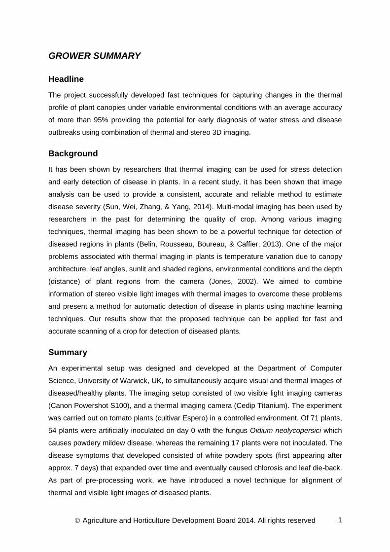
(a) Visible light image. (b) Thermal image. (c) Overlay of thermal image and the corresponding
visible image after alignment.
We also present technique for 3D modelling of diseased plants and compare it with the
existing state of the art methods. After pre-processing, we use machine learning techniques
and combine thermal and visible light image data with depth information to detect plants
infected with the tomato powdery mildew fungus Oidium neolycopersici. We present a
technique which can detect diseased plants using thermal and visible light imagery with an
average accuracy of detection more than 95%. In addition, we show that our method is
capable of identifying plants which were not originally inoculated with the fungus at the start
of the experiment but which subsequently developed disease through natural transmission.
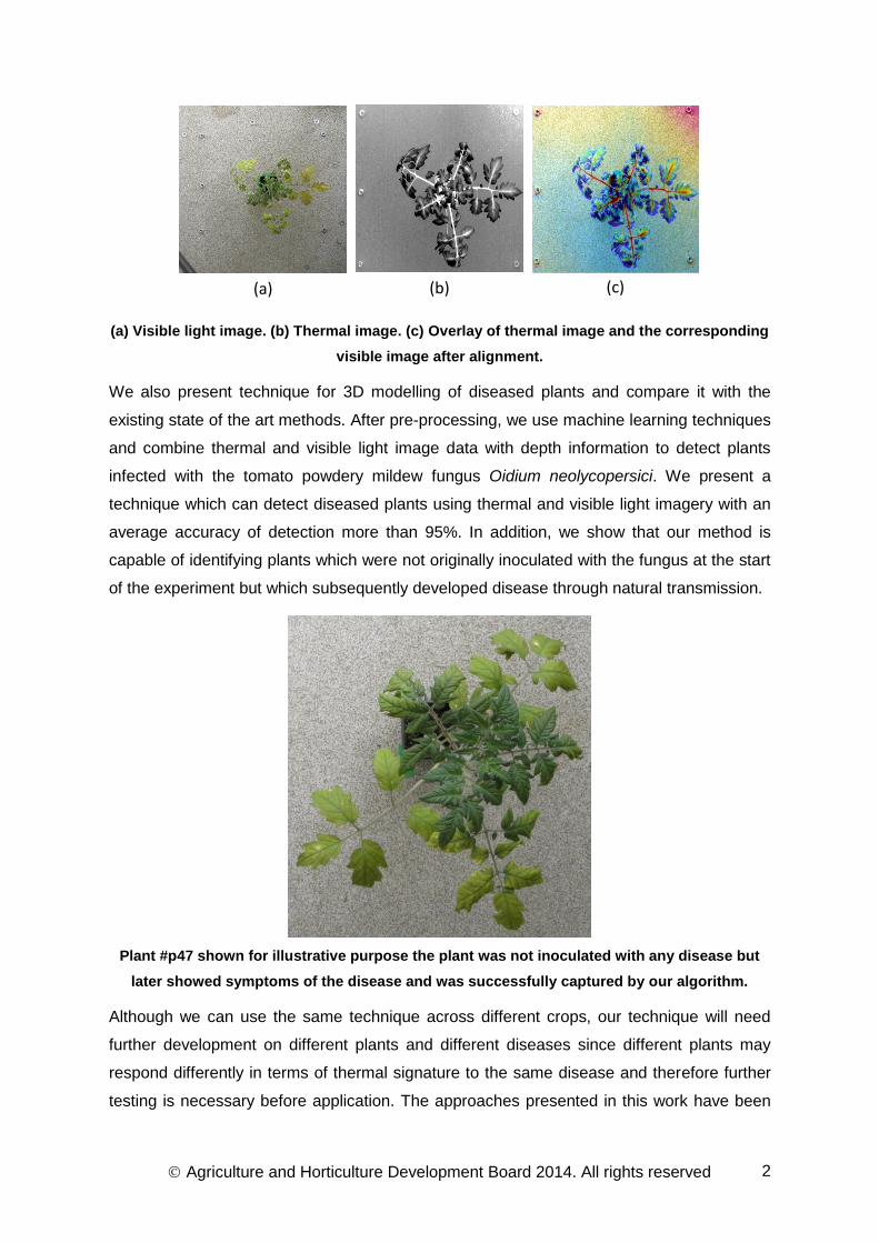
Plant #p47 shown for illustrative purpose the plant was not inoculated with any disease but
later showed symptoms of the disease and was successfully captured by our algorithm.
Although we can use the same technique across different crops, our technique will need
further development on different plants and different diseases since different plants may
respond differently in terms of thermal signature to the same disease and therefore further
testing is necessary before application. The approaches presented in this work have been
(a) (b) (c)
Agriculture and Horticulture Development Board 2014. All rights reserved
3
tested on spinach crop in real world environment and tomato plants in a controlled
environment. However, these approaches can be extended to different type of crop but
need to be tested on multiple types of disease with multiple control treatments at a larger
scale before they can be employed in a real world setting.
Financial Benefits
Early and accurate detection of stress and disease regions in a crop can help growers take
timely action against the disease/stress. In the previous report (CP60a, Year 2 report, 2013)
we had shown that we can efficiently and accurately identify stress regions in a crop with
the help of thermal imaging. Good irrigation strategies in turn can help the grower to get
optimal crop yield i.e., little or no loss of plants through over or under watering. In this
report, we have shown the strength of thermal and stereo visible light imaging systems for
early disease detection. In this report, we have shown that we can detect the onset of
powdery mildew disease before the visible symptoms appear, a disease which can cause
60% yield loss in extreme cases during epidemic onset1. Early disease detection can help to
avoid any possible crop yield loss. Thermal imaging can also be used for more efficient use
of fungicides by optimising spray quantity and timing or it can be used to spray only ‘disease
hotspots’ in glasshouse. The additional information which comes from 3D map has been
shown to increase the accuracy of disease detection and will definitely bring more financial
benefits to the grower. A good thermal imaging camera is available in the price range of
£15000 to £30000, with high end cameras having the ability to remotely transfer live
images, thermal and colour, via Wi-Fi networks on computer screens or tablet (e.g. iPad). A
camera can be mounted on a rig on moving boom e.g. on a water boom in Venlo type
glasshouses to scan the crop regions.
Action Points
Glasshouse businesses should consider options for installing an overhead system for
monitoring their crop with the help of a mounted thermal and colour imaging camera. The
cost of the imaging system is negligible compared to the financial benefits which can be
obtained using such kind of systems.
1 http://www.plantwise.org/KnowledgeBank/Datasheet.aspx?dsid=22075
Agriculture and Horticulture Development Board 2014. All rights reserved
1
SCIENCE SECTION
Introduction
Thermal imaging may assist in early detection of disease and stress in plants and canopies
and thus, allow for the design of timely control treatments (L Chaerle, Caeneghem, &
Messens, 1999; Idso, Jackson, Pinter Jr, Reginato, & Hatfield, 1981). Various studies show
that the temperature information captured in thermal images of plants may be affected by
several factors such as the amount of incident sunlight, the leaf angles and the distance
between the thermal camera and the plant, (Ju, Nebel, & Siebert, 2004; Stoll & Jones,
2007). Information about the effect of these factors can be obtained by using a stereo visual
and thermal imaging setup (Scharstein & Szeliski, 2002; Song, Wilson, Edmondson, &
Parsons, 2007). Therefore, early disease detection accuracy may be increased by
performing a joint analysis of temperature data from thermal images and imaging data from
visible light images (Cohen, Alchanatis, Prigojin, Levi, & Soroker, 2011; Leinonen & Jones,
2004). We aim to combine information of stereo visible light images with thermal images to
overcome these problems and present a method for automatic detection of disease in
plants using machine learning techniques. This report presents experiments and results
performed during the last year on joint analysis of thermal and stereo images of diseased
tomato plants.
Thermal imaging has good potential for early detection of plant disease, especially when the
disease directly affects transpiration rate. Early detection of disease is very important as
prompt intervention (e.g. through the application of fungicides or other control measures)
can control subsequent spread of disease which would result in reduced the quantity and
quality of crop yield (Erich-Christian Oerke, Gerhards, & Menz, 2010). Naidu et al. (Naidu,
Perry, Pierce, & Mekuria, 2009) used discriminant analysis to identify virus infected
grapevine (grapevine leafroll disease) using leaf reflectance spectra. The authors found
specific differences in wavelength intervals in the green, near infrared and mid-infrared
region and obtained a maximum accuracy of 81% in classification results. Chaerle et al. (L
Chaerle et al., 1999) studied tobacco infected with tobacco mosaic virus (TMV) and found
that sites of infection were 0.3-0.4°C warmer than the surrounding tissue hours before the
initial appearance of the necrotic lesions. They also observed a correlation between leaf
temperature and transpiration by thermography and steady-state porometry. In (Laury
Chaerle, Leinonen, Jones, & Van Der Straeten, 2007), Chaerle et al. studied the use of
thermal and chlorophyll fluorescence imaging in pre-symptomatic responses for diagnosis
of different diseases and to predict plant growth. The authors concluded that conventional
Agriculture and Horticulture Development Board 2014. All rights reserved
2
methods are time consuming and suitable for small number of plants, whereas imaging
techniques can be used to screen large number of plants for biotic and abiotic stress and to
predict the crop growth.
Oerke et al. (E-C Oerke, Steiner, Dehne, & Lindenthal, 2006) studied the changes in
metabolic processes and transpiration rate within cucumber leaves following infection by
Pseudoperonospora cubensis (downy mildew) and showed that healthy and infected leaves
can be discriminated even before symptoms appeared. The maximum temperature
difference (MTD) was found to be related to the severity of infection and could be used for
the discrimination of healthy leaves or those with downy mildew (Lindenthal, Steiner,
Dehne, & Oerke, 2005). In another study, Oerke et al. (E.-C. Oerke, Fröhling, & Steiner,
2011) investigated the effect of the fungus Venturia inaequalis on apple leaves and found
MTD to be strongly correlated with the size of infection sites. Stoll et al. (Stoll, Schultz, &
Berkelmann-Loehnertz, 2008) investigated the use of infrared thermography to study the
attack of Plasmopara viticola in grape vine leaves under varying water status conditions
while research on wheat canopies for detection of fungal diseases revealed that higher
temperature was observed for ears (containing the grain) infected with Fusarium (Lenthe,
Oerke, & Dehne, 2007; E-C Oerke & Steiner, 2010).
Thermal and visible light images are usually captured using different type of sensors from
different viewpoints and with different resolutions. As a pre-processing step before joint
analysis, thermal and visible light images of plants must be aligned so that the pixel
locations in both images correspond to the same physical locations in the plant. To the best
of our knowledge, there is no existing literature on automatic registration of thermal and
visible light images of diseased plants. However, in the past researchers have manually
registered thermal and colour images for multi-modal image analysis of plants (Leinonen &
Jones, 2004). Automatic registration of thermal and visible images of diseased plants is a
challenging task due to the fact that there is a mismatch in texture information and edge
information is often missing in the corresponding visible/thermal image. The reason for this
information mismatch is that the thermal profile of a leaf in a diseased plant can show
symptoms of disease before they visibly appear. In other words, a leaf with a smooth green
profile (colour) in the visible light image may have a textured profile in the thermal image
with a temperature higher or lower compared to that of the surrounding environment
because of the changes in the plant which visibly appear at a later stage.
Infrared thermal imaging has been previously employed in video surveillance e.g., traffic,
airport security, detection of concealed weapons, smoke detection and patient monitoring
(H. M. Chen, Lee, Rao, Slamani, & Varshney, 2005; Ju Han & Bhanu, 2007; Ju et al., 2004;
Agriculture and Horticulture Development Board 2014. All rights reserved
3
Verstockt et al., 2011). One approach for registration is to calibrate the stereo visual +
thermal imaging camera setup and use transformations to align the resulting images
(Krotosky & Trivedi, 2007; Torabi & Bilodeau, 2013; Zhao & Cheung, 2012). One
disadvantage of this approach is that the calibration parameters of the cameras may not be
readily available. In such cases, a possible solution is to align the thermal and visible light
images using exclusively image based information. Various researchers have proposed
methods that use line, edge and gradient information to register thermal and visible images
of scenes with strong edge and gradient information (Jungong Han, Pauwels, & de Zeeuw,
2013; Jungong Han, Pauwels, & Zeeuw, 2012; Kim, Lee, & Ra, 2008; J. H. Lee, Kim, Lee,
Kang, & Ra, 2010). In general, line, edge and corner based methods are reliable for images
of man-made environments, however they perform poorly on images of natural objects. Jarc
et al. (Jarc, Perš, Rogelj, Perše, & Kovacic, 2007) proposed a registration method based on
texture features; however, the method is not automatic and requires manual selection of
features. Other methods based on mutual information and cross correlation of image
patches rely on texture similarities between the two kinds of images (Bilodeau, St-Onge, &
Garnier, 2011; J. H. Lee et al., 2010; Torabi & Bilodeau, 2013). Since there is a high
probability that texture information may be missing in the corresponding visible/thermal
image(s) of diseased plants, methods based on mutual information and cross-correlation
may not be a good choice for registration.
Region-based methods, such as those based on silhouette extraction, usually provide more
reliable correspondence between visible and thermal images than feature based methods
(Bilodeau et al., 2011; H. Chen & Varshney, 2001; Verstockt et al., 2011). Bilodeau et al.
(Bilodeau et al., 2011) proposed registering thermal and visible images of people by
extracting features from human silhouettes. Torabi et al. (Torabi, Massé, & Bilodeau, 2012)
suggested a RANSAC trajectory-to-trajectory matching based registration method that
maximizes human silhouette overlap in video sequences. Han et al. (Ju Han & Bhanu,
2007) proposed a hierarchical genetic algorithm (HGA) for silhouette extraction using an
automatic registration method for human movement detection. The authors improve the
accuracy of the extracted human silhouette by combining silhouette and thermal/colour
information from coarsely registered thermal and visible images. Human body temperature
is generally higher than that of the background region and this characteristic has been used
by researchers in (H. Chen & Varshney, 2001; Verstockt et al., 2011) to extract human
silhouettes. However, in the case of thermal images of diseased plants, the temperature
profile does not exhibit this characteristic. It is possible that within the same plant the
temperature of different regions is higher or lower than that of the background. Another
common method for silhouette extraction in video sequences is background subtraction.
Agriculture and Horticulture Development Board 2014. All rights reserved
4
This method usually provides very good results because of the high frame rate of the
sequences and the fact that the background between two consecutive frames is usually
very similar. For the case of images of diseased plants, background subtraction is not
efficient due to the limited number of consecutive still images and the fact that there may be
a large interval between two consecutive still images.
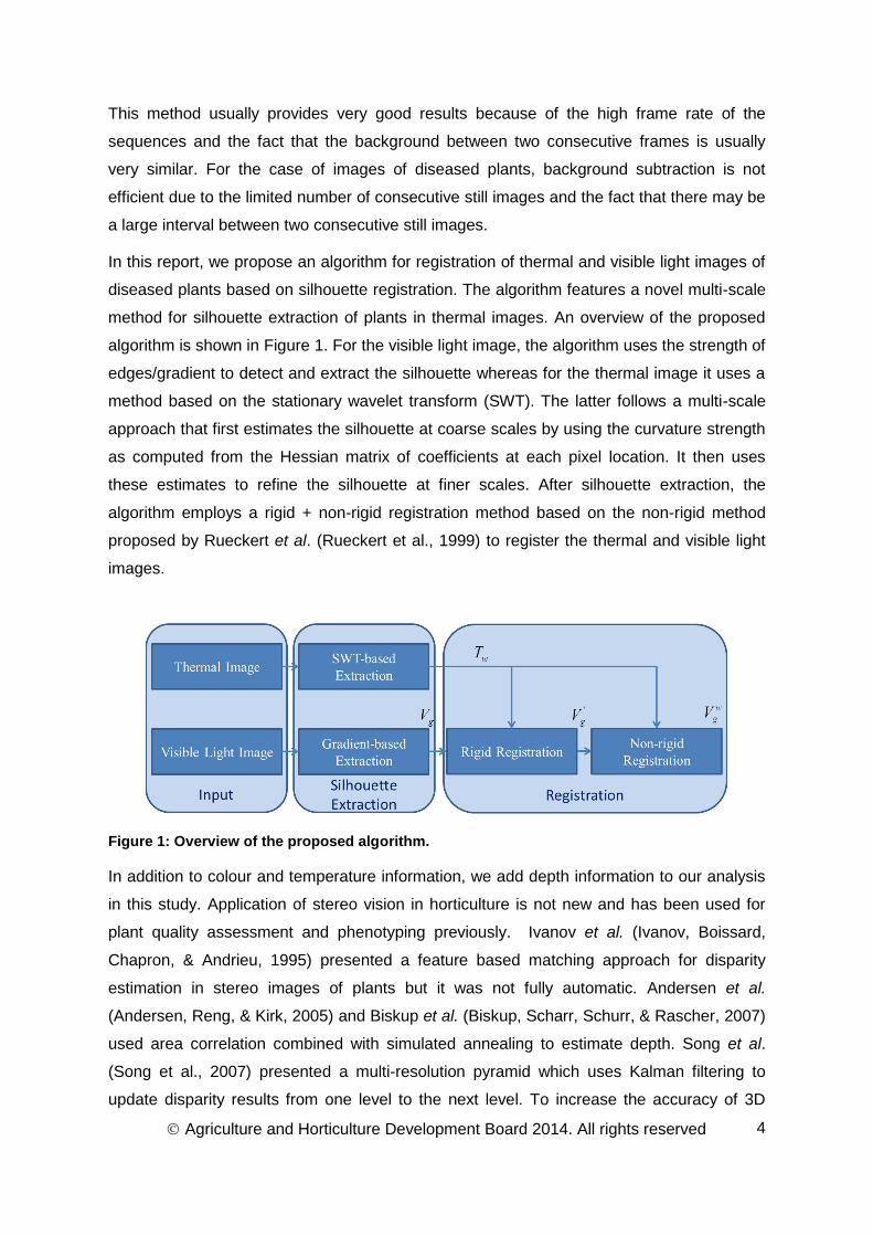
In this report, we propose an algorithm for registration of thermal and visible light images of
diseased plants based on silhouette registration. The algorithm features a novel multi-scale
method for silhouette extraction of plants in thermal images. An overview of the proposed
algorithm is shown in Figure 1. For the visible light image, the algorithm uses the strength of
edges/gradient to detect and extract the silhouette whereas for the thermal image it uses a
method based on the stationary wavelet transform (SWT). The latter follows a multi-scale
approach that first estimates the silhouette at coarse scales by using the curvature strength
as computed from the Hessian matrix of coefficients at each pixel location. It then uses
these estimates to refine the silhouette at finer scales. After silhouette extraction, the
algorithm employs a rigid + non-rigid registration method based on the non-rigid method
proposed by Rueckert et al. (Rueckert et al., 1999) to register the thermal and visible light
images.
Figure 1: Overview of the proposed algorithm.
In addition to colour and temperature information, we add depth information to our analysis
in this study. Application of stereo vision in horticulture is not new and has been used for
plant quality assessment and phenotyping previously. Ivanov et al. (Ivanov, Boissard,
Chapron, & Andrieu, 1995) presented a feature based matching approach for disparity
estimation in stereo images of plants but it was not fully automatic. Andersen et al.
(Andersen, Reng, & Kirk, 2005) and Biskup et al. (Biskup, Scharr, Schurr, & Rascher, 2007)
used area correlation combined with simulated annealing to estimate depth. Song et al.
(Song et al., 2007) presented a multi-resolution pyramid which uses Kalman filtering to
update disparity results from one level to the next level. To increase the accuracy of 3D
Agriculture and Horticulture Development Board 2014. All rights reserved
5
depth estimation, stereo vision has been combined by various researchers with Light
Detection and Ranging (LIDAR) technology (Omasa, Hosoi, & Konishi, 2007; Rosell &
Sanz, 2012). Here, we use a stereo visible imaging setup for depth estimation to avoid any
extra costs and computational burden being added to the setup by the addition of another
imaging system.
It is widely known that the thermal profile or the time interval between onset and visible
appearance of disease varies depending on the type of disease and the plant. This work is
a step towards making automatic detection of disease possible regardless of disease or
plant type. We present here a novel approach for automatic detection of diseased plants by
including depth information to thermal and visible light image data. We study the effect of a
fungus Oidium neolycopersici which causes powdery mildew in tomato plants and
investigate the effect of combining stereo visible imaging with thermal imaging on our ability
to detect the disease before appearance of visible symptoms. For depth estimation, we
compare six different disparity estimation algorithms and propose a method to estimate
smooth and accurate disparity maps with efficient computational cost. We propose two
different approaches to extract a novel feature set and show that it is capable of identifying
plants poised to be affected by the fungus during the experiment.
Materials and methods
Image Acquisition
An experimental setup was designed and developed at the Department of Computer
Science, University of Warwick, UK, to simultaneously acquire visual and thermal images of
diseased/healthy plants. The imaging setup consisted of two visible light imaging cameras
(Canon Powershot S100), and a thermal imaging camera (Cedip Titanium). The experiment
was carried out on 71 tomato plants (cultivar Espero) in a controlled environment at 20˚C
with thermal and stereo visible light images being collected for 14 consecutive days (day 0
to day13). Of these 71 plants, 54 plants were artificially inoculated on day 0 with the fungus
Oidium neolycopersici which causes powdery mildew disease, whereas the remaining 17
plants were not inoculated. Inoculation was carried out by spraying the tomato plants to run
off with a spore suspension of O. neolycopersici at a concentration of 1 x 10⁵ spores ml-1.
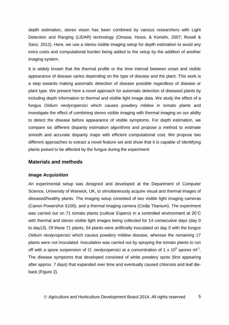
The disease symptoms that developed consisted of white powdery spots (first appearing
after approx. 7 days) that expanded over time and eventually caused chlorosis and leaf die-
back (Figure 2).
Agriculture and Horticulture Development Board 2014. All rights reserved
6
Figure 2: The appearance of disease symptoms with time on leaves of a diseased plant.
Silhouette Extraction
Thermal Image
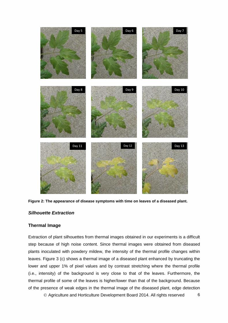
Extraction of plant silhouettes from thermal images obtained in our experiments is a difficult
step because of high noise content. Since thermal images were obtained from diseased
plants inoculated with powdery mildew, the intensity of the thermal profile changes within
leaves. Figure 3 (c) shows a thermal image of a diseased plant enhanced by truncating the
lower and upper 1% of pixel values and by contrast stretching where the thermal profile
(i.e., intensity) of the background is very close to that of the leaves. Furthermore, the
thermal profile of some of the leaves is higher/lower than that of the background. Because
of the presence of weak edges in the thermal image of the diseased plant, edge detection
Day 5 Day 6 Day 7
Day 8 Day 9 Day 10
Day 11 Day 12 Day 13
Agriculture and Horticulture Development Board 2014. All rights reserved
7
methods such as gradient, Canny edge detector, difference of Gaussian, Laplacian perform
poorly on thermal images. Based on this observation, we propose an approach that is
minimally affected by intensity changes within leaf.
It has been shown that the joint statistics of coefficients obtained after wavelet
transformation (WT) show strong correlation among object boundaries in thermal and visible
light images (Morris, Avidan, Matusik, & Pfister, 2007). Thermal images, therefore, capture
most of the object boundaries and thus WT can be used to extract silhouettes. Additionally,
WT has shown to be very efficient in reducing noise, improving mutli-scale analysis and
detecting edge direction information (Kong et al., 2006; Nashat, Abdullah, & Abdullah, 2011;
Olivo-Marin, 2002). Multi-scale wavelet-based methods have also shown to be efficient in
fusing thermal and visible light images (S. Chen, Su, Zhang, & Tian, 2008; Pajares &
Manuel de la Cruz, 2004). In this work, we present a multi-scale wavelet-based method to
extract plant silhouettes in thermal images. We use the stationary wavelet transform (SWT),
which is similar to the discrete wavelet transform (DWT) except that it does not use down
sampling. As a result, the resulting frequency sub-bands generated have the same size as
the input image and contain coefficients that are redundant and correlated across different
scales (Nason & Silverman, 1995). Our multi-scale SWT-based method uses the Haar filter
to first decompose the thermal image into a number of sub-bands.
For an image of m×n pixels, it computes a matrix equivalent to the matrix of second
derivatives (Hessian) at each pixel location (Morse, 2000; Nashat et al., 2011):
, ,
| | | |
| | | |
ijs ijs
i j sijs ijs
V D
D H
(1)
Figure 3: (a) Example visible light image; (b) silhouette extracted from visible light image (Vg)
using the gradient-based method; (c) corresponding thermal image (enhanced by truncating
the upper and lower 1% pixel values and by contrast stretching); and (d) silhouette extracted
from thermal image (Tw) using the SWT-based method.
where are the horizontal, vertical and diagonal coefficients, respectively, at
scale s and pixel location ( ); scale corresponds to the first level of decomposition.
(a) (b) (c) (d)
Agriculture and Horticulture Development Board 2014. All rights reserved
8
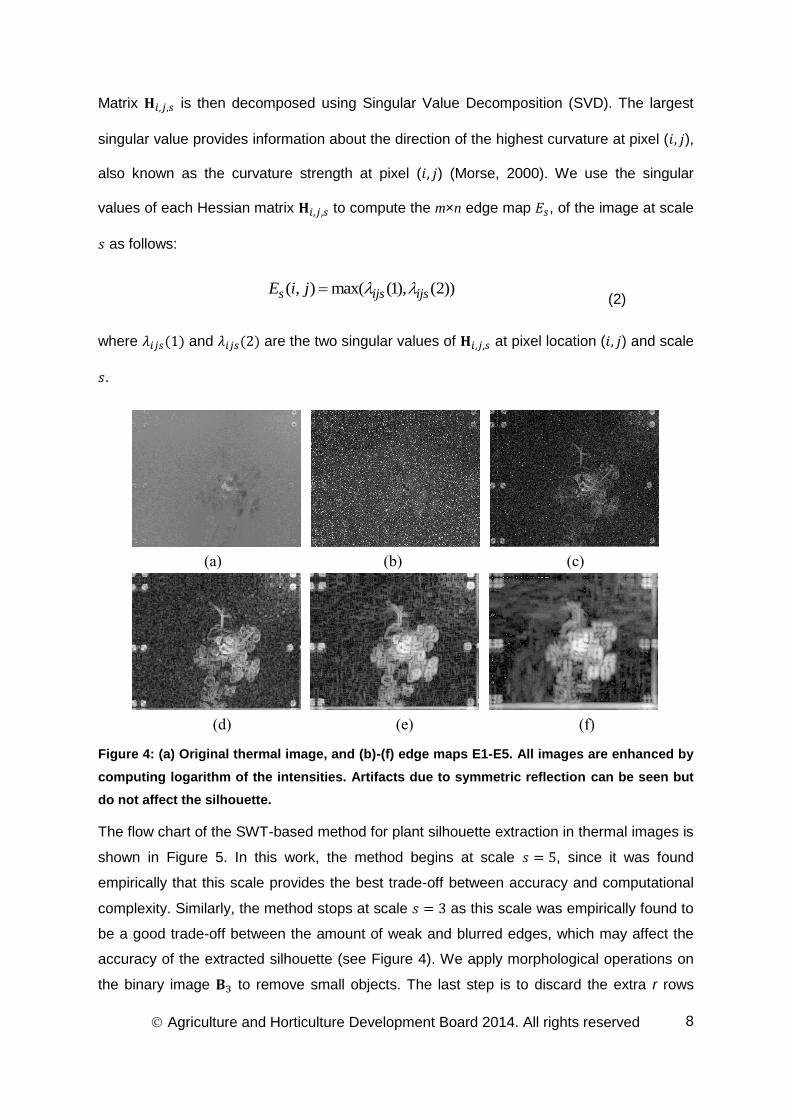
Matrix is then decomposed using Singular Value Decomposition (SVD). The largest
singular value provides information about the direction of the highest curvature at pixel ( ),
also known as the curvature strength at pixel ( ) (Morse, 2000). We use the singular
values of each Hessian matrix to compute the m×n edge map , of the image at scale
as follows:
( , ) max( (1), (2))s ijs ijsE i j
(2)
where and are the two singular values of at pixel location ( ) and scale
.
Figure 4: (a) Original thermal image, and (b)-(f) edge maps E1-E5. All images are enhanced by
computing logarithm of the intensities. Artifacts due to symmetric reflection can be seen but
do not affect the silhouette.
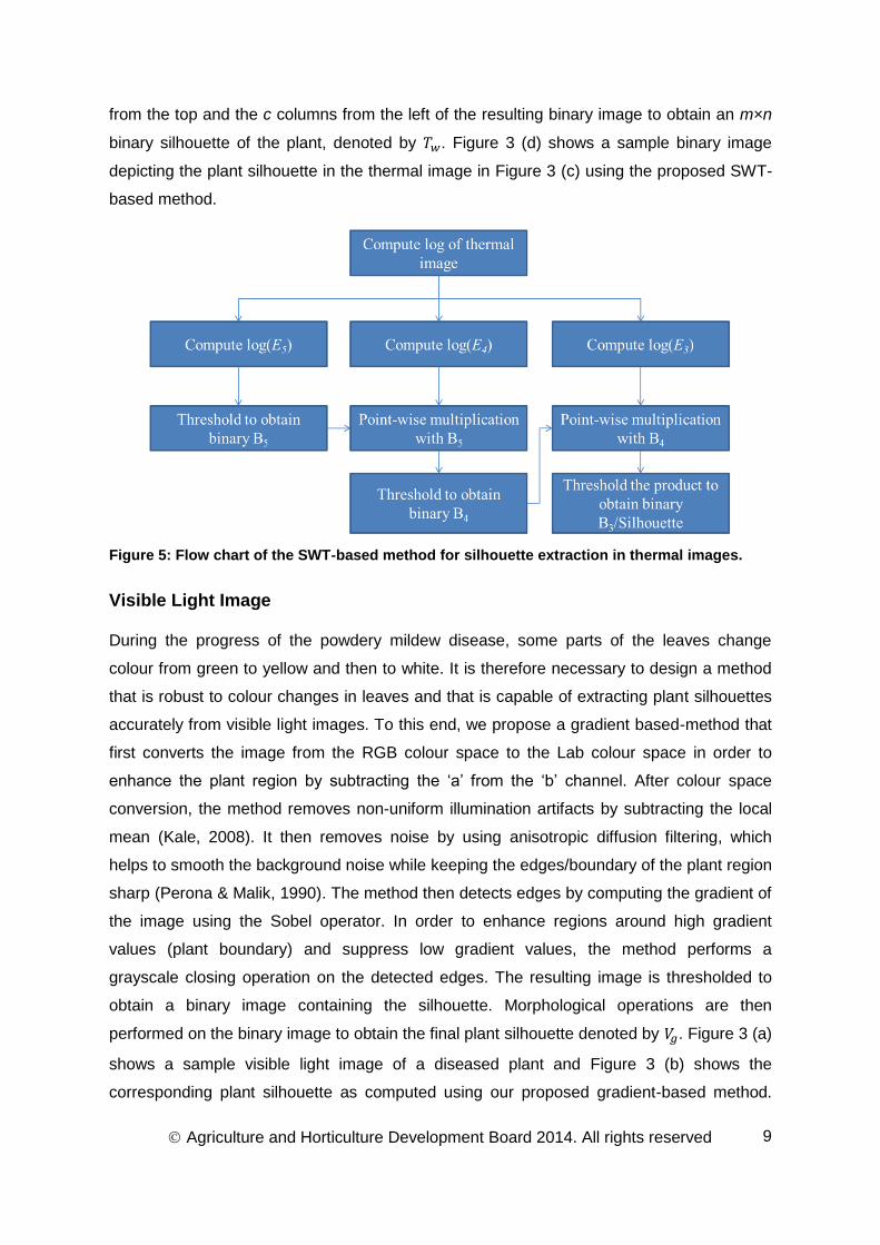
The flow chart of the SWT-based method for plant silhouette extraction in thermal images is
shown in Figure 5. In this work, the method begins at scale , since it was found
empirically that this scale provides the best trade-off between accuracy and computational
complexity. Similarly, the method stops at scale as this scale was empirically found to
be a good trade-off between the amount of weak and blurred edges, which may affect the
accuracy of the extracted silhouette (see Figure 4). We apply morphological operations on
the binary image to remove small objects. The last step is to discard the extra r rows
(b) (c)
(d) (e) (f)
(a)
Agriculture and Horticulture Development Board 2014. All rights reserved
9
from the top and the c columns from the left of the resulting binary image to obtain an m×n
binary silhouette of the plant, denoted by . Figure 3 (d) shows a sample binary image
depicting the plant silhouette in the thermal image in Figure 3 (c) using the proposed SWT-
based method.
Figure 5: Flow chart of the SWT-based method for silhouette extraction in thermal images.
Visible Light Image
During the progress of the powdery mildew disease, some parts of the leaves change
colour from green to yellow and then to white. It is therefore necessary to design a method
that is robust to colour changes in leaves and that is capable of extracting plant silhouettes
accurately from visible light images. To this end, we propose a gradient based-method that
first converts the image from the RGB colour space to the Lab colour space in order to
enhance the plant region by subtracting the ‘a’ from the ‘b’ channel. After colour space
conversion, the method removes non-uniform illumination artifacts by subtracting the local
mean (Kale, 2008). It then removes noise by using anisotropic diffusion filtering, which
helps to smooth the background noise while keeping the edges/boundary of the plant region
sharp (Perona & Malik, 1990). The method then detects edges by computing the gradient of
the image using the Sobel operator. In order to enhance regions around high gradient
values (plant boundary) and suppress low gradient values, the method performs a
grayscale closing operation on the detected edges. The resulting image is thresholded to
obtain a binary image containing the silhouette. Morphological operations are then
performed on the binary image to obtain the final plant silhouette denoted by . Figure 3 (a)
shows a sample visible light image of a diseased plant and Figure 3 (b) shows the
corresponding plant silhouette as computed using our proposed gradient-based method.
Agriculture and Horticulture Development Board 2014. All rights reserved
10
Note that the main motivation to use this method in visible light images, as opposed to the
SWT-based method, is the low computationally complexity and good results. We further
discuss this in results and discussions section.
Registration
The goal of registration is to align the thermal and visible light images in such a way that the
same pixel locations in both the images correspond to same physical location in the plant.
Our particular registration method is a two-step process: rigid and non-rigid registration. In
rigid registration, a similarity transformation is parameterised by four degrees of freedom. A
general similarity transformation matrix for a 2D image can be written as:
2 1
2 1
cos sin.
sin cos
x
y
tx xS
ty y
(3)
where S is the scale factor, is the angle of rotation along the z-axis, and xt and yt are
the shifts in the x and y directions, respectively. The transformation in Eq. (5) maps a point
1 1( , )x y in a floating image to a corresponding point 2 2( , )x y in a static image. In our case,
the binary image depicting the plant silhouette from the visible light image is the floating
image and the binary image depicting the plant silhouette from the thermal image is the
static image. The rigid registration step first finds the centroid of the plant silhouette in both
the thermal and visible images. It then calculates the difference between centroid locations
and shifts the floating image by a number of pixels equal to this difference. It uses the sum
of absolute differences as a cost function and an optimized pattern search algorithm (Audet
& Dennis, 2002) to search for the best approximation of similarity transformation between
the two plant silhouettes. The search space range is chosen to be [0.9, 1.1] for scale factor
S, [-0.1˚, 0.1˚] for angle α, and [-100, 100] pixels for translations ( ,x yt t ). The resulting
registered visible image silhouette obtained after applying similarity transformation is
denoted by '
gV .
After rigid registration, the second step performs non-rigid registration using a free-form
deformation (FFD) model based on multilevel cubic B-Spline approximation proposed by
Rueckert et al. (Kroon, 2011; S. Lee, Wolberg, & Shin, 1997; Rueckert et al., 1999). FFD
models deform an object by manipulating an underlying mesh of control points . For an
image of m×n pixels, let {( , ) | 0 ,0 }x y x m y n be the image domain on the xy-
plane, and ij be the value of the ij-th control point on lattice represented by a x yn n
mesh with uniform spacing . The FFD approximation function can then be written as
Agriculture and Horticulture Development Board 2014. All rights reserved
11
3 3
,
0 0
( , ) ( ) ( )k l i k j l
k l
x y B t B u
T (4)
where / 1xi x n , / 1yj y n , / /x xt x n x n , / /y yu y n y n and kB and
lB represent cubic B-spline basis functions. This second step uses the hierarchical multi-
level B-spline approximation proposed in (S. Lee et al., 1997) and an implementation of the
limited memory Broyden–Fletcher–Goldfarb–Shanno algorithm (L-BFGS) by Dirk-Jan Kroon
as the optimization function (Kroon, 2011). The similarity measure used here is the Sum of
Squared Differences (SSD):
' ' 2
,
( , ( )) ( ( , ) ( ( , )))similarity w g w g
x y
C T V T x y V x y
(5)
where '( )gV is the plant silhouette from the visible light image after applying transformation
( , )x yT to '
gV ; wT and '
gV are the silhouette of the thermal image and registered visible light
image, respectively, as obtained by the rigid registration step.
Depth Estimation
To add depth information to the set of features which can be collected from registered
thermal and visible light images, we use disparity between the stereo image pair. For a
stereo vision setup depth (Z) can be related to disparity (d) by /d fB Z , where f is focal
length of the lens of the camera and B is the baseline which can be defined as the distance
between the centres of left and right camera lens. In this work, we propose a disparity
estimation algorithm for estimation of smooth and accurate disparity maps and compare the
results with five state of the art existing methods. We selected these five algorithms for our
study based on three criteria 1) they represent major disparity estimation schemes, 2) these
methods have been used in the past for comparison studies (Scharstein & Szeliski, 2002),
and 3) they produce acceptable results on the plant images. The goal is to present a
method which produces accurate and smooth disparity map, and is less sensitive to the
background noise and colour variation in the diseased plants.
The first two methods in our list are based on block based matching. The first method based
on block based stereo matching (BSM) was proposed in (Konolige, 1998). BSM takes
Laplacian of Gaussian (LoG) transform of the stereo images and then uses absolute
differences to find the matching blocks. A Multi-Resolution Stereo Matching (MRSM) was
designed for surface modelling of plants in (Song et al., 2007). The algorithm first divides
the image into overlapping blocks at each level of a multi-resolution pyramid and then uses
Agriculture and Horticulture Development Board 2014. All rights reserved
12
a variation of the Birchfield and Tomasi (BT) cost function to match the corresponding
blocks (Birchfield & Tomasi, 1999).
Graph-cut based Stereo Matching (GCM) (V. Kolmogorov & Zabih, 2001) is a widely used
disparity estimation method. This algorithm defines a global energy function and minimises
the energy function using graph cuts (Boykov & Kolmogorov, 2004; Boykov, Veksler, &
Zabih, 2001; V. Kolmogorov & Zabih, 2001; Vladimir Kolmogorov & Zabih, 2002). The
algorithm initially defines a unique disparity α and then iteratively searches for an α which
minimises the energy function. The fourth method non-local cost aggregation (NCA) (Yang,
2012) uses the concept of bilateral filter by weighting the pixel intensity differences with
intensity edges and provides a non-local solution by aggregating the cost on a tree structure
derived from the stereo image pair.
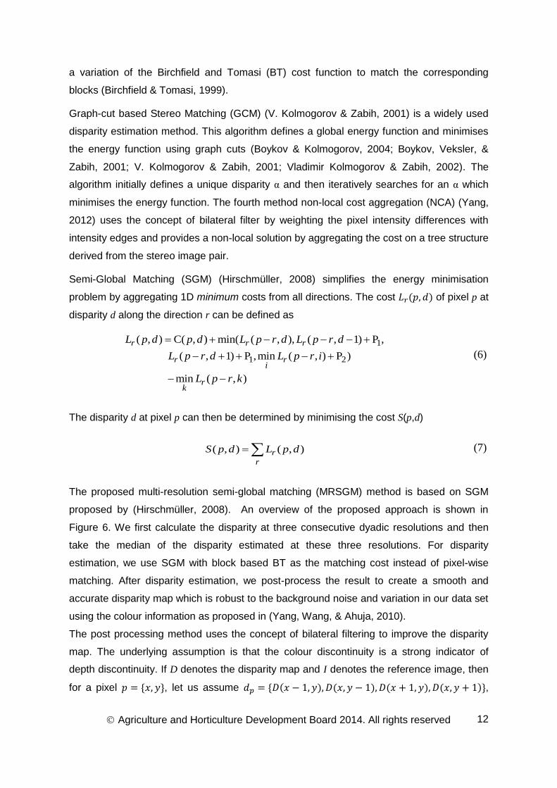
Semi-Global Matching (SGM) (Hirschmüller, 2008) simplifies the energy minimisation
problem by aggregating 1D minimum costs from all directions. The cost of pixel p at
disparity d along the direction r can be defined as
1
1 2
( , ) C( , ) min( ( , ), ( , 1) P ,
( , 1) P ,min ( , ) P )
min ( , )
r r r
r ri
rk
L p d p d L p r d L p r d
L p r d L p r i
L p r k
(6)
The disparity d at pixel p can then be determined by minimising the cost S(p,d)
( , ) ( , )rr
S p d L p d (7)
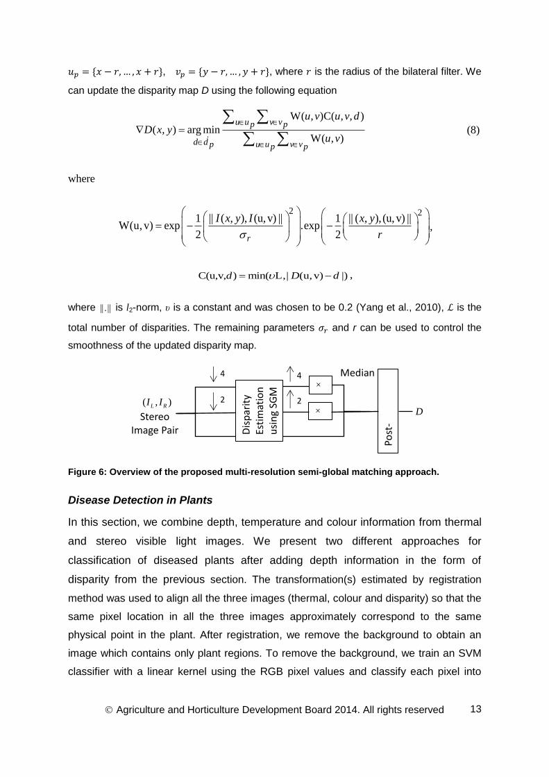
The proposed multi-resolution semi-global matching (MRSGM) method is based on SGM
proposed by (Hirschmüller, 2008). An overview of the proposed approach is shown in
Figure 6. We first calculate the disparity at three consecutive dyadic resolutions and then
take the median of the disparity estimated at these three resolutions. For disparity
estimation, we use SGM with block based BT as the matching cost instead of pixel-wise
matching. After disparity estimation, we post-process the result to create a smooth and
accurate disparity map which is robust to the background noise and variation in our data set
using the colour information as proposed in (Yang, Wang, & Ahuja, 2010).
The post processing method uses the concept of bilateral filtering to improve the disparity
map. The underlying assumption is that the colour discontinuity is a strong indicator of
depth discontinuity. If D denotes the disparity map and I denotes the reference image, then
for a pixel , let us assume ,
Agriculture and Horticulture Development Board 2014. All rights reserved
13
, , where is the radius of the bilateral filter. We
can update the disparity map D using the following equation
W( , )C( , , )
( , ) arg minW( , )
u u v vp p
d d u u v vp p p
u v u v d
D x yu v
(8)
where
2 21 || ( , ), (u, v) || 1 || ( , ), (u, v) ||
W(u, v) exp .exp2 2r
I x y I x y
r
,
C(u,v, ) min( ,| (u,v) |)d D d L ,
where || . || is l2-norm, υ is a constant and was chosen to be 0.2 (Yang et al., 2010), is the
total number of disparities. The remaining parameters and r can be used to control the
smoothness of the updated disparity map.
Figure 6: Overview of the proposed multi-resolution semi-global matching approach.
Disease Detection in Plants
In this section, we combine depth, temperature and colour information from thermal
and stereo visible light images. We present two different approaches for
classification of diseased plants after adding depth information in the form of
disparity from the previous section. The transformation(s) estimated by registration
method was used to align all the three images (thermal, colour and disparity) so that the
same pixel location in all the three images approximately correspond to the same
physical point in the plant. After registration, we remove the background to obtain an
image which contains only plant regions. To remove the background, we train an SVM
classifier with a linear kernel using the RGB pixel values and classify each pixel into
Stereo Image Pair
( , )L RI I
4
2
Dis
par
ity
Esti
mat
ion
usi
ng
SGM
4
2
×
4
×
2
Median
Post
-P
roce
ssin
g D
Agriculture and Horticulture Development Board 2014. All rights reserved
14
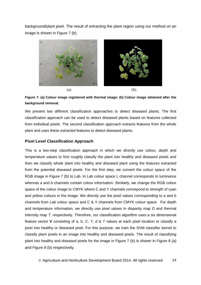
background/plant pixel. The result of extracting the plant region using our method on an
image is shown in Figure 7 (b).
Figure 7: (a) Colour image registered with thermal image; (b) Colour image obtained after the
background removal.
We present two different classification approaches to detect diseased plants. The first
classification approach can be used to detect diseased plants based on features collected
from individual pixels. The second classification approach extracts features from the whole
plant and uses these extracted features to detect diseased plants.
Pixel Level Classification Approach
This is a two-step classification approach in which we directly use colour, depth and
temperature values to first roughly classify the plant into healthy and diseased pixels and
then we classify whole plant into healthy and diseased plant using the features extracted
from the potential diseased pixels. For the first step, we convert the colour space of the
RGB image in Figure 7 (b) to Lab. In Lab colour space L channel corresponds to luminance
whereas a and b channels contain colour information. Similarly, we change the RGB colour
space of the colour image to CMYK where C and Y channels correspond to strength of cyan
and yellow colours in the image. We directly use the pixel values corresponding to a and b
channels from Lab colour space and C & Y channels from CMYK colour space. For depth
and temperature information, we directly use pixel values in disparity map D and thermal
intensity map T, respectively. Therefore, our classification algorithm uses a six dimensional
feature vector V consisting of a, b, C, Y, d & T values at each pixel location to classify a
pixel into healthy or diseased pixel. For this purpose, we train the SVM classifier kernel to
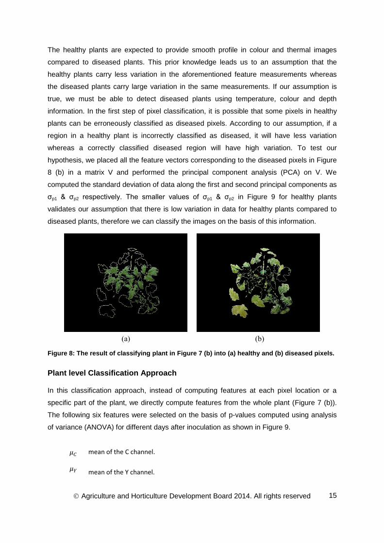
classify plant pixels in an image into healthy and diseased pixels. The result of classifying
plant into healthy and diseased pixels for the image in Figure 7 (b) is shown in Figure 8 (a)
and Figure 8 (b) respectively.
(a) (b)
Agriculture and Horticulture Development Board 2014. All rights reserved
15
The healthy plants are expected to provide smooth profile in colour and thermal images
compared to diseased plants. This prior knowledge leads us to an assumption that the
healthy plants carry less variation in the aforementioned feature measurements whereas
the diseased plants carry large variation in the same measurements. If our assumption is
true, we must be able to detect diseased plants using temperature, colour and depth
information. In the first step of pixel classification, it is possible that some pixels in healthy
plants can be erroneously classified as diseased pixels. According to our assumption, if a
region in a healthy plant is incorrectly classified as diseased, it will have less variation
whereas a correctly classified diseased region will have high variation. To test our
hypothesis, we placed all the feature vectors corresponding to the diseased pixels in Figure
8 (b) in a matrix V and performed the principal component analysis (PCA) on V. We
computed the standard deviation of data along the first and second principal components as
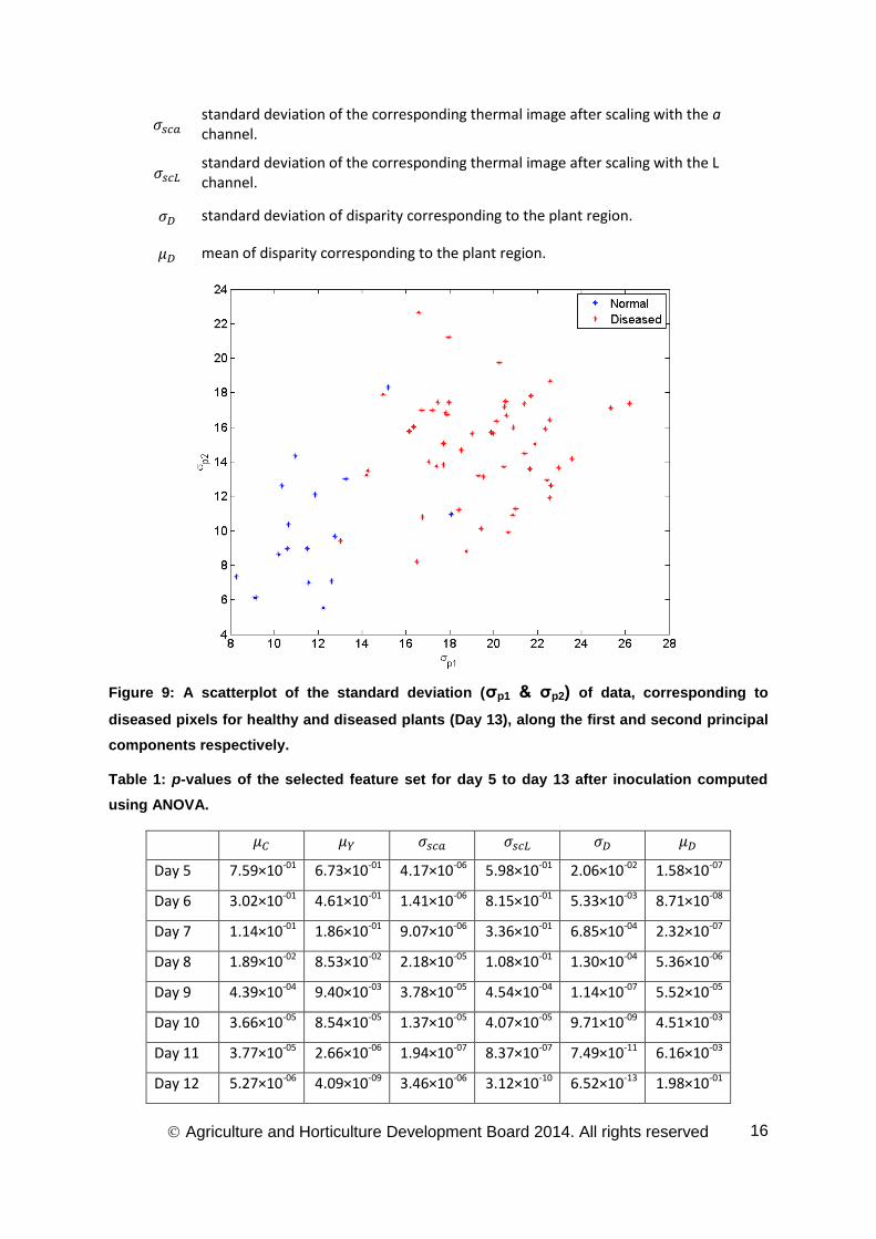
σp1 & σp2 respectively. The smaller values of σp1 & σp2 in Figure 9 for healthy plants
validates our assumption that there is low variation in data for healthy plants compared to
diseased plants, therefore we can classify the images on the basis of this information.
Figure 8: The result of classifying plant in Figure 7 (b) into (a) healthy and (b) diseased pixels.
Plant level Classification Approach
In this classification approach, instead of computing features at each pixel location or a
specific part of the plant, we directly compute features from the whole plant (Figure 7 (b)).
The following six features were selected on the basis of p-values computed using analysis
of variance (ANOVA) for different days after inoculation as shown in Figure 9.
mean of the C channel.
mean of the Y channel.
(a) (b)
Agriculture and Horticulture Development Board 2014. All rights reserved
16
standard deviation of the corresponding thermal image after scaling with the a channel.
standard deviation of the corresponding thermal image after scaling with the L channel.
standard deviation of disparity corresponding to the plant region.
mean of disparity corresponding to the plant region.
Figure 9: A scatterplot of the standard deviation (σp1 & σp2) of data, corresponding to
diseased pixels for healthy and diseased plants (Day 13), along the first and second principal
components respectively.
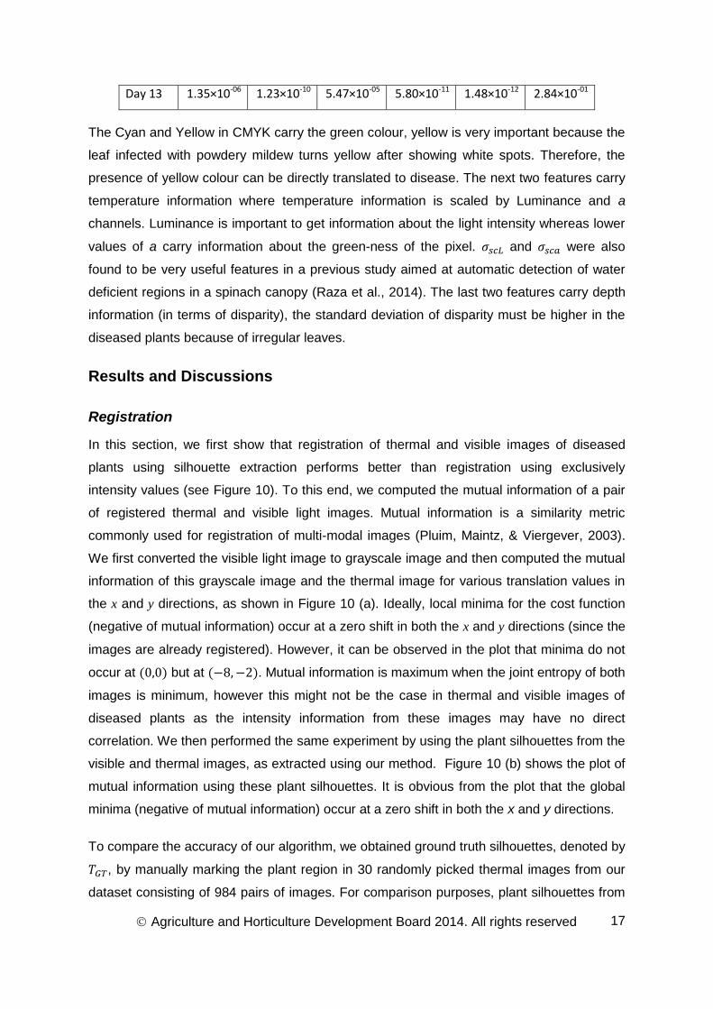
Table 1: p-values of the selected feature set for day 5 to day 13 after inoculation computed
using ANOVA.
Day 5 7.59×10-01 6.73×10-01 4.17×10-06 5.98×10-01 2.06×10-02 1.58×10-07
Day 6 3.02×10-01 4.61×10-01 1.41×10-06 8.15×10-01 5.33×10-03 8.71×10-08
Day 7 1.14×10-01 1.86×10-01 9.07×10-06 3.36×10-01 6.85×10-04 2.32×10-07
Day 8 1.89×10-02 8.53×10-02 2.18×10-05 1.08×10-01 1.30×10-04 5.36×10-06
Day 9 4.39×10-04 9.40×10-03 3.78×10-05 4.54×10-04 1.14×10-07 5.52×10-05
Day 10 3.66×10-05 8.54×10-05 1.37×10-05 4.07×10-05 9.71×10-09 4.51×10-03
Day 11 3.77×10-05 2.66×10-06 1.94×10-07 8.37×10-07 7.49×10⁻¹¹ 6.16×10-03
Day 12 5.27×10-06 4.09×10-09 3.46×10-06 3.12×10⁻¹⁰ 6.52×10⁻¹³ 1.98×10-01
Agriculture and Horticulture Development Board 2014. All rights reserved
17
Day 13 1.35×10-06 1.23×10⁻¹⁰ 5.47×10-05 5.80×10⁻¹¹ 1.48×10⁻¹² 2.84×10-01
The Cyan and Yellow in CMYK carry the green colour, yellow is very important because the
leaf infected with powdery mildew turns yellow after showing white spots. Therefore, the
presence of yellow colour can be directly translated to disease. The next two features carry
temperature information where temperature information is scaled by Luminance and a
channels. Luminance is important to get information about the light intensity whereas lower
values of a carry information about the green-ness of the pixel. and were also
found to be very useful features in a previous study aimed at automatic detection of water
deficient regions in a spinach canopy (Raza et al., 2014). The last two features carry depth
information (in terms of disparity), the standard deviation of disparity must be higher in the
diseased plants because of irregular leaves.
Results and Discussions
Registration
In this section, we first show that registration of thermal and visible images of diseased
plants using silhouette extraction performs better than registration using exclusively
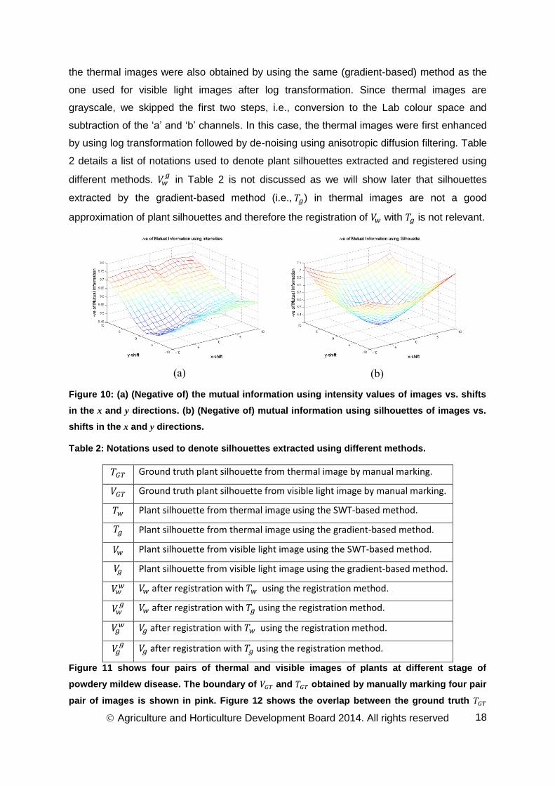
intensity values (see Figure 10). To this end, we computed the mutual information of a pair
of registered thermal and visible light images. Mutual information is a similarity metric
commonly used for registration of multi-modal images (Pluim, Maintz, & Viergever, 2003).
We first converted the visible light image to grayscale image and then computed the mutual
information of this grayscale image and the thermal image for various translation values in
the x and y directions, as shown in Figure 10 (a). Ideally, local minima for the cost function
(negative of mutual information) occur at a zero shift in both the x and y directions (since the
images are already registered). However, it can be observed in the plot that minima do not
occur at but at . Mutual information is maximum when the joint entropy of both
images is minimum, however this might not be the case in thermal and visible images of
diseased plants as the intensity information from these images may have no direct
correlation. We then performed the same experiment by using the plant silhouettes from the
visible and thermal images, as extracted using our method. Figure 10 (b) shows the plot of
mutual information using these plant silhouettes. It is obvious from the plot that the global
minima (negative of mutual information) occur at a zero shift in both the x and y directions.
To compare the accuracy of our algorithm, we obtained ground truth silhouettes, denoted by
, by manually marking the plant region in 30 randomly picked thermal images from our
dataset consisting of 984 pairs of images. For comparison purposes, plant silhouettes from
Agriculture and Horticulture Development Board 2014. All rights reserved
18
the thermal images were also obtained by using the same (gradient-based) method as the
one used for visible light images after log transformation. Since thermal images are
grayscale, we skipped the first two steps, i.e., conversion to the Lab colour space and
subtraction of the ‘a’ and ‘b’ channels. In this case, the thermal images were first enhanced
by using log transformation followed by de-noising using anisotropic diffusion filtering. Table
2 details a list of notations used to denote plant silhouettes extracted and registered using
different methods. in Table 2 is not discussed as we will show later that silhouettes
extracted by the gradient-based method (i.e., ) in thermal images are not a good
approximation of plant silhouettes and therefore the registration of with is not relevant.
Figure 10: (a) (Negative of) the mutual information using intensity values of images vs. shifts
in the x and y directions. (b) (Negative of) mutual information using silhouettes of images vs.
shifts in the x and y directions.
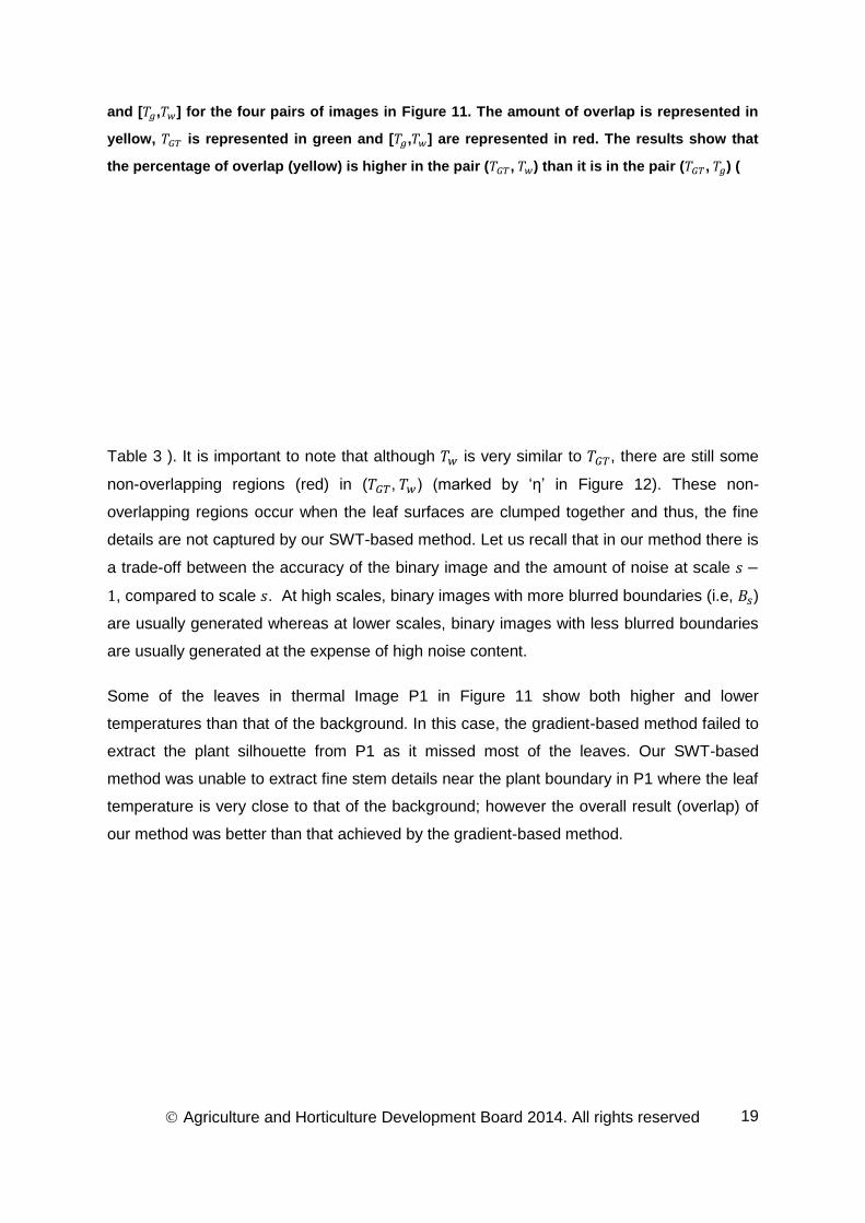
Table 2: Notations used to denote silhouettes extracted using different methods.
Ground truth plant silhouette from thermal image by manual marking.
Ground truth plant silhouette from visible light image by manual marking.
Plant silhouette from thermal image using the SWT-based method.
Plant silhouette from thermal image using the gradient-based method.
Plant silhouette from visible light image using the SWT-based method.
Plant silhouette from visible light image using the gradient-based method.
after registration with using the registration method.
after registration with using the registration method.
after registration with using the registration method.
after registration with using the registration method.
Figure 11 shows four pairs of thermal and visible images of plants at different stage of
powdery mildew disease. The boundary of and obtained by manually marking four pair
pair of images is shown in pink. Figure 12 shows the overlap between the ground truth
(a) (b)
Agriculture and Horticulture Development Board 2014. All rights reserved
19
and [ , ] for the four pairs of images in Figure 11. The amount of overlap is represented in
yellow, is represented in green and [ , ] are represented in red. The results show that
the percentage of overlap (yellow) is higher in the pair ( , ) than it is in the pair ( , ) (
Table 3 ). It is important to note that although is very similar to , there are still some
non-overlapping regions (red) in ( , ) (marked by ‘η’ in Figure 12). These non-
overlapping regions occur when the leaf surfaces are clumped together and thus, the fine
details are not captured by our SWT-based method. Let us recall that in our method there is
a trade-off between the accuracy of the binary image and the amount of noise at scale
, compared to scale . At high scales, binary images with more blurred boundaries (i.e, )
are usually generated whereas at lower scales, binary images with less blurred boundaries
are usually generated at the expense of high noise content.
Some of the leaves in thermal Image P1 in Figure 11 show both higher and lower
temperatures than that of the background. In this case, the gradient-based method failed to
extract the plant silhouette from P1 as it missed most of the leaves. Our SWT-based
method was unable to extract fine stem details near the plant boundary in P1 where the leaf
temperature is very close to that of the background; however the overall result (overlap) of
our method was better than that achieved by the gradient-based method.
Agriculture and Horticulture Development Board 2014. All rights reserved
20
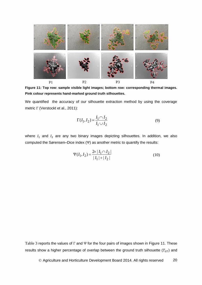
Figure 11: Top row: sample visible light images; bottom row: corresponding thermal images.
Pink colour represents hand-marked ground truth silhouettes.
We quantified the accuracy of our silhouette extraction method by using the coverage
metric (Verstockt et al., 2011):
1 2
1 21 2
( , )I I
I II I
(9)
where and are any two binary images depicting silhouettes. In addition, we also
computed the Sørensen–Dice index ( ) as another metric to quantify the results:
1 2
1 21 2
2 | |( , )
| | | |
I II I
I I
(10)
Table 3 reports the values of and for the four pairs of images shown in Figure 11. These
results show a higher percentage of overlap between the ground truth silhouette ( ) and
P2 P3 P1 P4
Agriculture and Horticulture Development Board 2014. All rights reserved
21
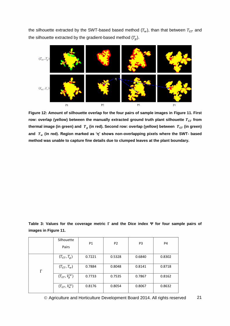
the silhouette extracted by the SWT-based based method ( ), than that between and
the silhouette extracted by the gradient-based method ( ).
Figure 12: Amount of silhouette overlap for the four pairs of sample images in Figure 11. First
row: overlap (yellow) between the manually extracted ground truth plant silhouette from
thermal image (in green) and (in red). Second row: overlap (yellow) between (in green)
and (in red). Region marked as ‘η’ shows non-overlapping pixels where the SWT- based
method was unable to capture fine details due to clumped leaves at the plant boundary.
Table 3: Values for the coverage metric and the Dice index for four sample pairs of
images in Figure 11.
Silhouette
Pairs P1 P2 P3 P4
( , 0.7221 0.5328 0.6840 0.8302
( , ) 0.7884 0.8048 0.8141 0.8718
( , 0.7733 0.7535 0.7867 0.8162
( , ) 0.8176 0.8054 0.8067 0.8632
Agriculture and Horticulture Development Board 2014. All rights reserved
22
( , ) 0.8459 0.89 0.8911 0.8372
( , 0.8386 0.6952 0.8123 0.9072
( , ) 0.8817 0.8919 0.8975 0.9315
( , 0.8722 0.8594 0.8806 0.8988
( , ) 0.8997 0.8922 0.8930 0.9266
( , ) 0.9165 0.9418 0.9424 0.9114
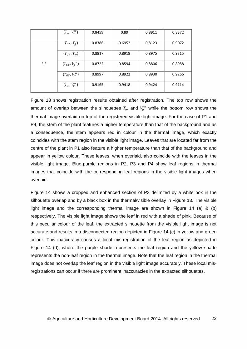
Figure 13 shows registration results obtained after registration. The top row shows the
amount of overlap between the silhouettes and while the bottom row shows the
thermal image overlaid on top of the registered visible light image. For the case of P1 and
P4, the stem of the plant features a higher temperature than that of the background and as
a consequence, the stem appears red in colour in the thermal image, which exactly
coincides with the stem region in the visible light image. Leaves that are located far from the
centre of the plant in P1 also feature a higher temperature than that of the background and
appear in yellow colour. These leaves, when overlaid, also coincide with the leaves in the
visible light image. Blue-purple regions in P2, P3 and P4 show leaf regions in thermal
images that coincide with the corresponding leaf regions in the visible light images when
overlaid.
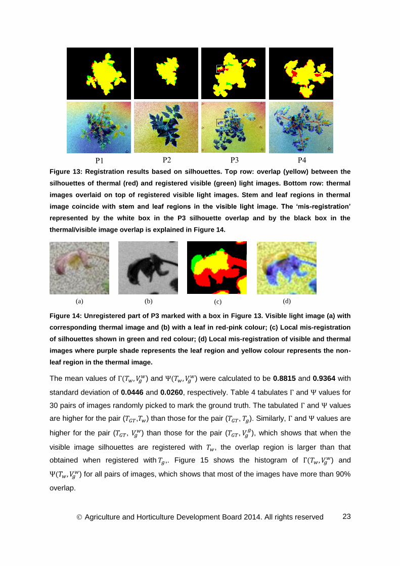
Figure 14 shows a cropped and enhanced section of P3 delimited by a white box in the
silhouette overlap and by a black box in the thermal/visible overlay in Figure 13. The visible
light image and the corresponding thermal image are shown in Figure 14 (a) & (b)
respectively. The visible light image shows the leaf in red with a shade of pink. Because of
this peculiar colour of the leaf, the extracted silhouette from the visible light image is not
accurate and results in a disconnected region depicted in Figure 14 (c) in yellow and green
colour. This inaccuracy causes a local mis-registration of the leaf region as depicted in
Figure 14 (d), where the purple shade represents the leaf region and the yellow shade
represents the non-leaf region in the thermal image. Note that the leaf region in the thermal
image does not overlap the leaf region in the visible light image accurately. These local mis-
registrations can occur if there are prominent inaccuracies in the extracted silhouettes.
Agriculture and Horticulture Development Board 2014. All rights reserved
23
Figure 13: Registration results based on silhouettes. Top row: overlap (yellow) between the
silhouettes of thermal (red) and registered visible (green) light images. Bottom row: thermal
images overlaid on top of registered visible light images. Stem and leaf regions in thermal
image coincide with stem and leaf regions in the visible light image. The ‘mis-registration’
represented by the white box in the P3 silhouette overlap and by the black box in the
thermal/visible image overlap is explained in Figure 14.
Figure 14: Unregistered part of P3 marked with a box in Figure 13. Visible light image (a) with
corresponding thermal image and (b) with a leaf in red-pink colour; (c) Local mis-registration
of silhouettes shown in green and red colour; (d) Local mis-registration of visible and thermal
images where purple shade represents the leaf region and yellow colour represents the non-
leaf region in the thermal image.
The mean values of )
and
) were calculated to be 0.8815 and 0.9364 with
standard deviation of 0.0446 and 0.0260, respectively. Table 4 tabulates and values for
30 pairs of images randomly picked to mark the ground truth. The tabulated and values
are higher for the pair ( , ) than those for the pair ( , ). Similarly, and values are
higher for the pair ( , ) than those for the pair ( ,
), which shows that when the
visible image silhouettes are registered with , the overlap region is larger than that
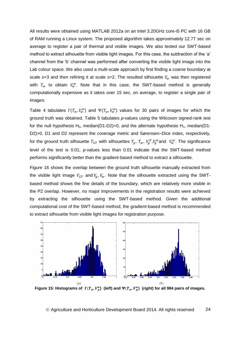
obtained when registered with ,. Figure 15 shows the histogram of )
and
) for all pairs of images, which shows that most of the images have more than 90%
overlap.
P2 P3 P1 P4
(b) (c) (a) (d)
Agriculture and Horticulture Development Board 2014. All rights reserved
24
All results were obtained using MATLAB 2012a on an Intel 3.20GHz core-i5 PC with 16 GB
of RAM running a Linux system. The proposed algorithm takes approximately 12.77 sec on
average to register a pair of thermal and visible images. We also tested our SWT-based
method to extract silhouette from visible light images. For this case, the subtraction of the ‘a’
channel from the ‘b’ channel was performed after converting the visible light image into the
Lab colour space. We also used a multi-scale approach by first finding a coarse boundary at
scale s=3 and then refining it at scale s=2. The resulted silhouette was then registered
with to obtain . Note that in this case, the SWT-based method is generally
computationally expensive as it takes over 15 sec, on average, to register a single pair of
images.
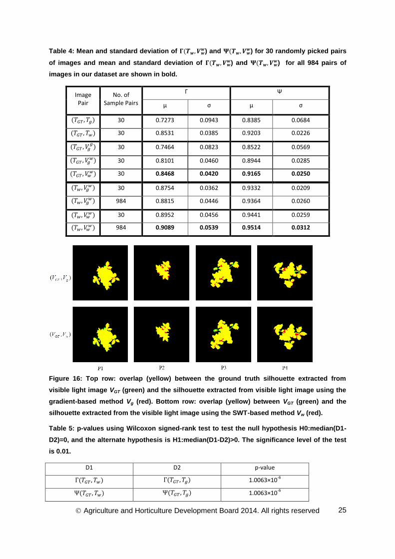
Table 4 tabulates )
and
) values for 30 pairs of images for which the
ground truth was obtained. Table 5 tabulates p-values using the Wilcoxon signed-rank test
for the null hypothesis H0, median(D1-D2)=0, and the alternate hypothesis H1, median(D1-
D2)>0. D1 and D2 represent the coverage metric and Sørensen–Dice index, respectively,
for the ground truth silhouette with silhouettes , , ,
and . The significance
level of the test is 0.01; p-values less than 0.01 indicate that the SWT-based method
performs significantly better than the gradient-based method to extract a silhouette.
Figure 16 shows the overlap between the ground truth silhouette manually extracted from
the visible light image and , . Note that the silhouette extracted using the SWT-
based method shows the fine details of the boundary, which are relatively more visible in
the P2 overlap. However, no major improvements in the registration results were achieved
by extracting the silhouette using the SWT-based method. Given the additional
computational cost of the SWT-based method, the gradient-based method is recommended
to extract silhouette from visible light images for registration purpose.
Figure 15: Histograms of
) (left) and
) (right) for all 984 pairs of images.
Agriculture and Horticulture Development Board 2014. All rights reserved
25
Table 4: Mean and standard deviation of )
and
) for 30 randomly picked pairs
of images and mean and standard deviation of )
and
) for all 984 pairs of
images in our dataset are shown in bold.
Image Pair
No. of Sample Pairs
Γ Ψ
µ σ µ σ
30 0.7273 0.0943 0.8385 0.0684
30 0.8531 0.0385 0.9203 0.0226
30 0.7464 0.0823 0.8522 0.0569
30 0.8101 0.0460 0.8944 0.0285
30 0.8468 0.0420 0.9165 0.0250
30 0.8754 0.0362 0.9332 0.0209
984 0.8815 0.0446 0.9364 0.0260
30 0.8952 0.0456 0.9441 0.0259
984 0.9089 0.0539 0.9514 0.0312
Figure 16: Top row: overlap (yellow) between the ground truth silhouette extracted from
visible light image VGT (green) and the silhouette extracted from visible light image using the
gradient-based method Vg (red). Bottom row: overlap (yellow) between VGT (green) and the
silhouette extracted from the visible light image using the SWT-based method Vw (red).
Table 5: p-values using Wilcoxon signed-rank test to test the null hypothesis H0:median(D1-
D2)=0, and the alternate hypothesis is H1:median(D1-D2)>0. The significance level of the test
is 0.01.
D1 D2 p-value
1.0063×10⁻⁶
1.0063×10⁻⁶
Agriculture and Horticulture Development Board 2014. All rights reserved
26
9.4802×10
-4
9.4802×10
-4
6.1686×10⁻⁷
6.1686×10⁻⁷
6.1686×10
-7
6.1686×10
-7
Depth Estimation
All the algorithms and results presented in this section were generated using a machine
running Windows 7 on an Intel Core i3-2120 (3.3 GHz) CPU with 3GB RAM (665 MHz). The
code for MRSM (provided by the author) was implemented in MATLAB 2013a, whereas the
C/C++ implementation of GCM and NCA were downloaded from the author’s websites. We
used OpenCV library to implement SGM in C++ for our experiments. The BSM and
MRSGM were partially implemented in C++ and partially in MATLAB 2013a, where the post
processing algorithm in MRSGM uses C++ implementation by (Yang et al., 2010).
For BSM, we chose 11×11 block size and for MRSM, we used 16×16 with 2 pyramid levels
for our experiments. For GCM, NCA and SGM, we chose default parameters provided by
the authors. Finally, we chose 5×5 block-based BT as cost function and r=3, for
MRSGM. All the parameters specified above other than the default parameters were
chosen on the basis of their good results on stereo images of diseased plants.
To validate our algorithm we have compared the results of the proposed MRSGM with the
remaining five algorithms in the appendix A. We have shown that our algorithm not only
produces decent results on standard test datasets but is also computationally efficient
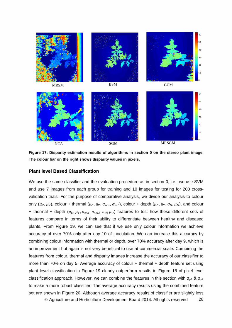
compared to other algorithms. Figure 17 compares results of all the six algorithms on our
dataset. It shows that MRSM performed poorly on the plant images and was found to be
very sensitive to the background noisy pattern in the image. From the results on test images
from Middlebury dataset (Appendix A), we know that GCM and NCA produce accurate
disparity maps but in the case of plant images these two algorithms were found to be highly
sensitive to the noise content in the image. GCM is slow and produces artifacts along the
scan lines on the plant images. NCA produces false disparity maps in the region which
belong to the background. The NCA algorithm divides the image into regions and assumes
a constant disparity throughout this region. This introduces artifacts which can be observed
in NCA result. BSM and SGM results were found to be less sensitive to background noise
but the disparity map produced by the algorithms were not smooth and showed small
peaks/patches around some pixels which were inconsistent with the neighbouring disparity.
When compared to all the other algorithms, MRSGM not only produced smooth disparity

Agriculture and Horticulture Development Board 2014. All rights reserved
27
maps but was also found to be less sensitive to the noise content. Although GCM and NCA
performed well on the test datasets, our plant images with relatively more background noise
than the Middlebury images proved to be quite challenging for these algorithms. In addition,
GCM and NCA were calculated to be very slow compared to the proposed MRSGM which
was found to be not only less sensitive to the noisy pattern but also produced smooth and
accurate disparity maps.
Classification Results
In the following sections, we present results of classification of diseased plants using pixel
level and plant level classification approaches.
Pixel level Classification
From the total of 71 plants, 54 plants were diseased and 17 plants were healthy (not
inoculated with the fungus). To test the strength of our features, we used SVM classifier.
We ran 200 cross-validation trials and tested the classifier using random pairs of training
and testing data. In each trial, we randomly picked 17 out of 54 diseased plants for
classification purpose. Once the number of diseased and healthy plants was equal, we
randomly picked 7 out of 17 healthy and diseased plants each for training purpose and the
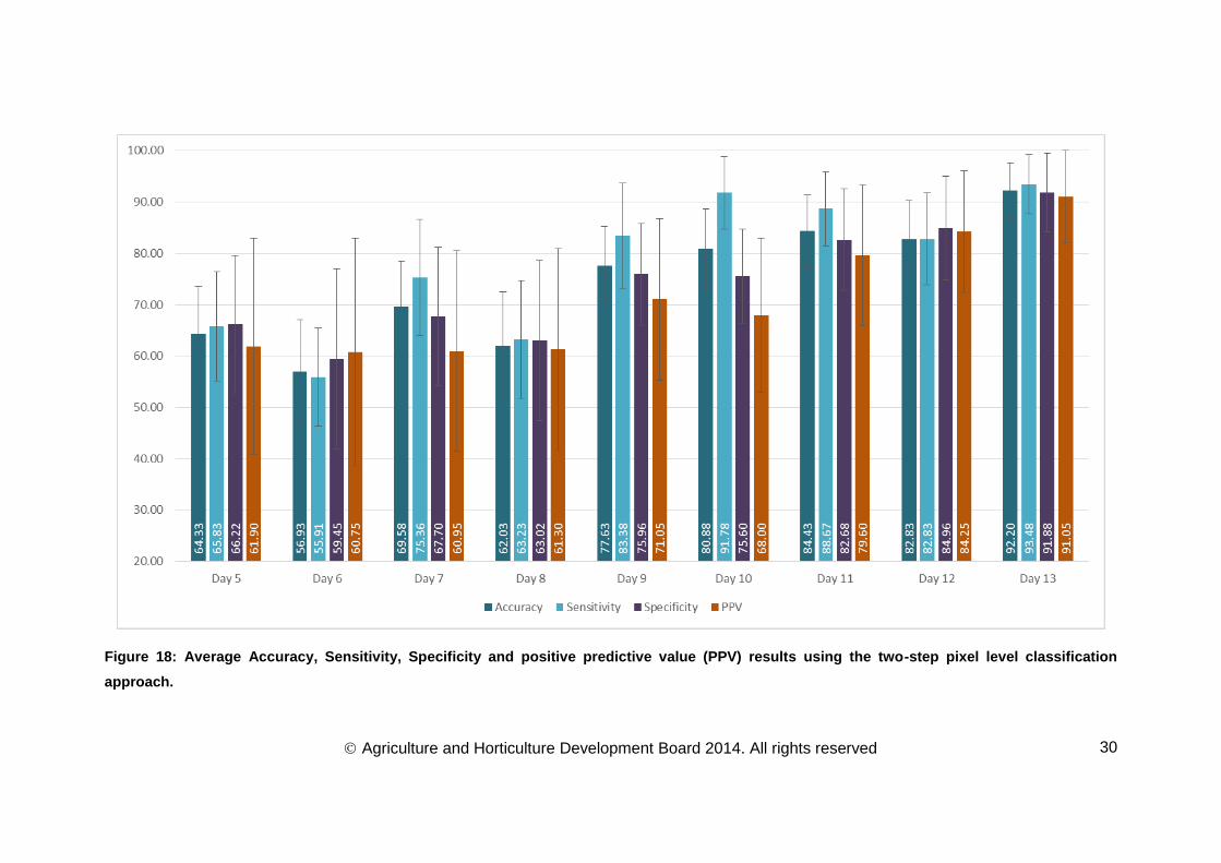
remaining 10 for testing the classifier. The classification results of the proposed classifier for
200 trials in terms of average accuracy, sensitivity, specificity and positive predictive value
(PPV) are shown in Figure 18. The disease starts to appear 7 days after inoculation and,
therefore, we concentrate on classification results for day 5 to 13 after inoculation. Figure 18
indicates that we can achieve an average accuracy of more than 75%, 9 days after
inoculation. The highest average accuracy achieved in this case is on day 13 i.e., 92.20%,
which is very significant. However, as the disease starts to appear 7 days after inoculation
detecting the disease after day 9 is not very beneficial at the commercial level as it might
spread across the crop. In the next section, we show that we can improve the accuracy of
detection of diseased plants using the features collected at plant level.
Agriculture and Horticulture Development Board 2014. All rights reserved
28
Figure 17: Disparity estimation results of algorithms in section 0 on the stereo plant image.
The colour bar on the right shows disparity values in pixels.
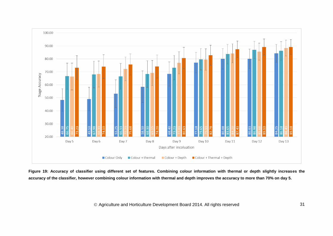
Plant level Based Classification
We use the same classifier and the evaluation procedure as in section 0, i.e., we use SVM
and use 7 images from each group for training and 10 images for testing for 200 cross-
validation trials. For the purpose of comparative analysis, we divide our analysis to colour
only ( , ), colour + thermal ( , , , ), colour + depth ( , , , ), and colour
+ thermal + depth ( , , , , , ) features to test how these different sets of
features compare in terms of their ability to differentiate between healthy and diseased
plants. From Figure 19, we can see that if we use only colour information we achieve
accuracy of over 70% only after day 10 of inoculation. We can increase this accuracy by
combining colour information with thermal or depth, over 70% accuracy after day 9, which is
an improvement but again is not very beneficial to use at commercial scale. Combining the
features from colour, thermal and disparity images increase the accuracy of our classifier to
more than 70% on day 5. Average accuracy of colour + thermal + depth feature set using
plant level classification in Figure 19 clearly outperform results in Figure 18 of pixel level
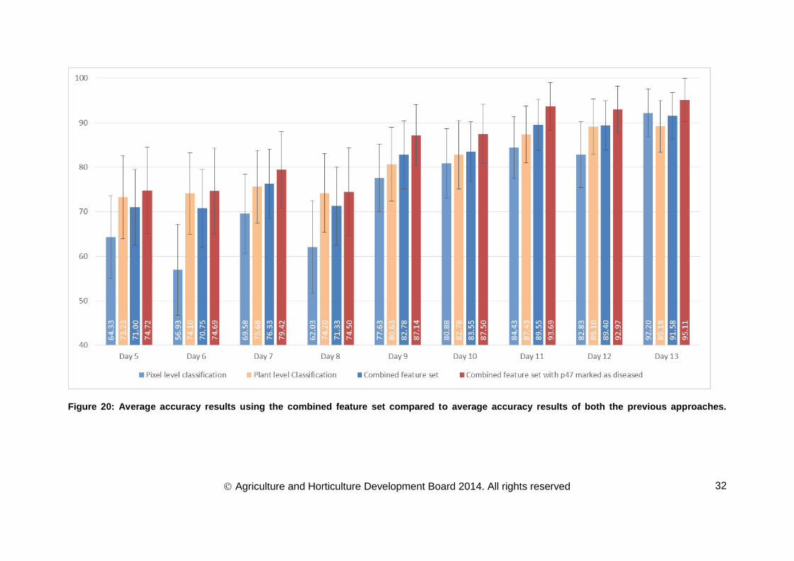
classification approach. However, we can combine the features in this section with σp1 & σp2
to make a more robust classifier. The average accuracy results using the combined feature
set are shown in Figure 20. Although average accuracy results of classifier are slightly less
MRSM BSM GCM
NCA SGM MRSGM
Agriculture and Horticulture Development Board 2014. All rights reserved
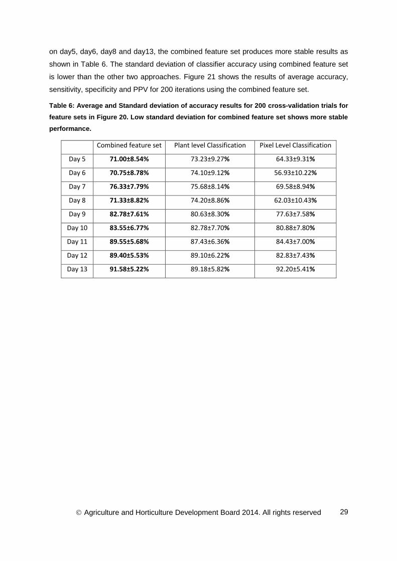
29
on day5, day6, day8 and day13, the combined feature set produces more stable results as
shown in Table 6. The standard deviation of classifier accuracy using combined feature set
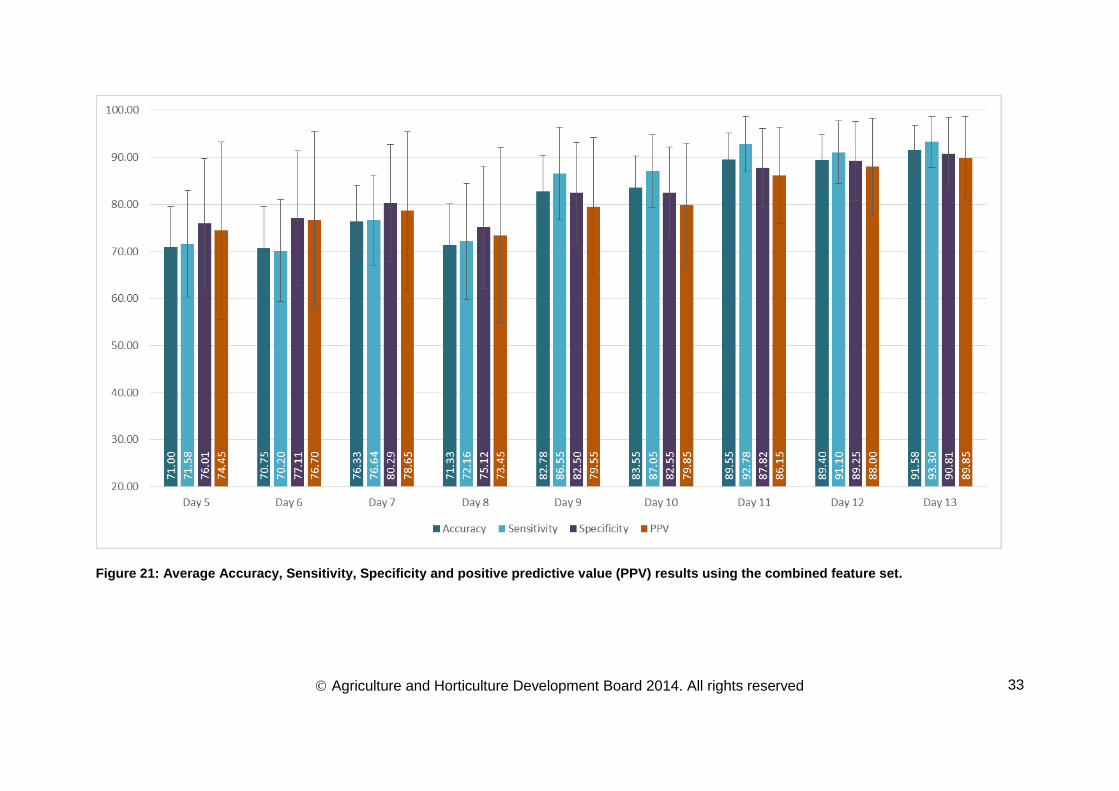
is lower than the other two approaches. Figure 21 shows the results of average accuracy,
sensitivity, specificity and PPV for 200 iterations using the combined feature set.
Table 6: Average and Standard deviation of accuracy results for 200 cross-validation trials for
feature sets in Figure 20. Low standard deviation for combined feature set shows more stable
performance.
Combined feature set Plant level Classification Pixel Level Classification
Day 5 71.00±8.54% 73.23±9.27% 64.33±9.31%
Day 6 70.75±8.78% 74.10±9.12% 56.93±10.22%
Day 7 76.33±7.79% 75.68±8.14% 69.58±8.94%
Day 8 71.33±8.82% 74.20±8.86% 62.03±10.43%
Day 9 82.78±7.61% 80.63±8.30% 77.63±7.58%
Day 10 83.55±6.77% 82.78±7.70% 80.88±7.80%
Day 11 89.55±5.68% 87.43±6.36% 84.43±7.00%
Day 12 89.40±5.53% 89.10±6.22% 82.83±7.43%
Day 13 91.58±5.22% 89.18±5.82% 92.20±5.41%
Agriculture and Horticulture Development Board 2014. All rights reserved
30
Figure 18: Average Accuracy, Sensitivity, Specificity and positive predictive value (PPV) results using the two-step pixel level classification
approach.
Agriculture and Horticulture Development Board 2014. All rights reserved
31
Figure 19: Accuracy of classifier using different set of features. Combining colour information with thermal or depth slightly increases the
accuracy of the classifier, however combining colour information with thermal and depth improves the accuracy to more than 70% on day 5.
Agriculture and Horticulture Development Board 2014. All rights reserved
32
Figure 20: Average accuracy results using the combined feature set compared to average accuracy results of both the previous approaches.
Agriculture and Horticulture Development Board 2014. All rights reserved
33
Figure 21: Average Accuracy, Sensitivity, Specificity and positive predictive value (PPV) results using the combined feature set.
Agriculture and Horticulture Development Board 2014. All rights reserved
34
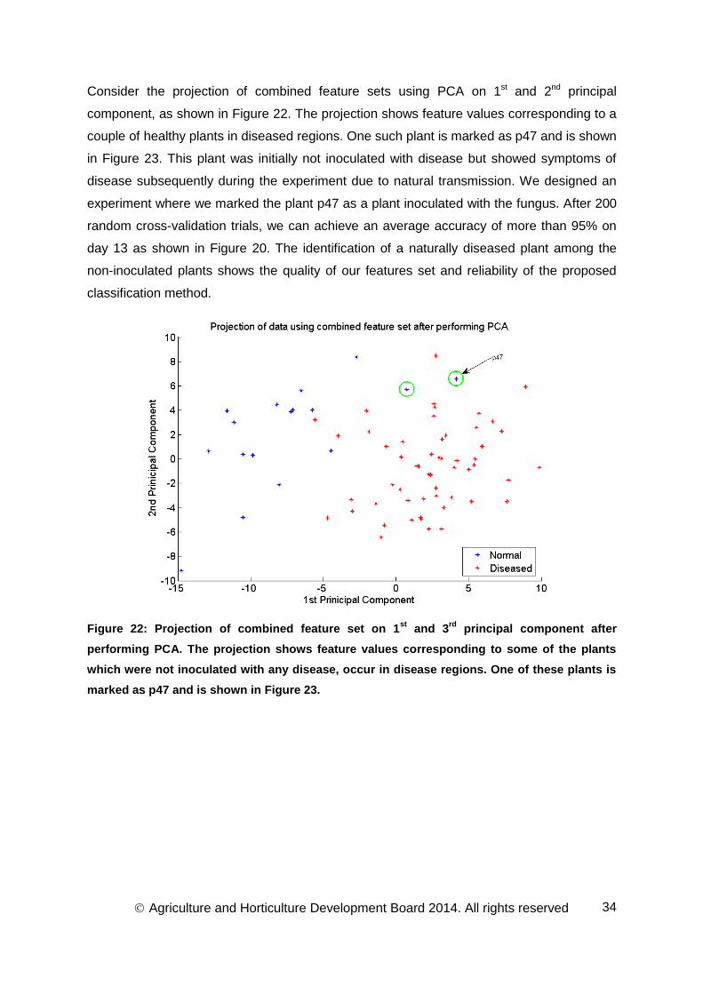
Consider the projection of combined feature sets using PCA on 1st and 2nd principal
component, as shown in Figure 22. The projection shows feature values corresponding to a
couple of healthy plants in diseased regions. One such plant is marked as p47 and is shown
in Figure 23. This plant was initially not inoculated with disease but showed symptoms of
disease subsequently during the experiment due to natural transmission. We designed an
experiment where we marked the plant p47 as a plant inoculated with the fungus. After 200
random cross-validation trials, we can achieve an average accuracy of more than 95% on
day 13 as shown in Figure 20. The identification of a naturally diseased plant among the
non-inoculated plants shows the quality of our features set and reliability of the proposed
classification method.
Figure 22: Projection of combined feature set on 1st
and 3rd
principal component after
performing PCA. The projection shows feature values corresponding to some of the plants
which were not inoculated with any disease, occur in disease regions. One of these plants is
marked as p47 and is shown in Figure 23.
Agriculture and Horticulture Development Board 2014. All rights reserved
35
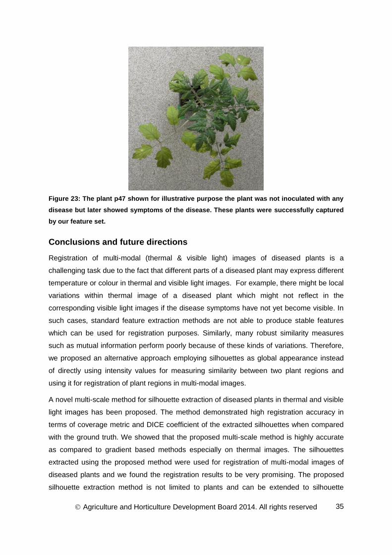
Figure 23: The plant p47 shown for illustrative purpose the plant was not inoculated with any
disease but later showed symptoms of the disease. These plants were successfully captured
by our feature set.
Conclusions and future directions
Registration of multi-modal (thermal & visible light) images of diseased plants is a
challenging task due to the fact that different parts of a diseased plant may express different
temperature or colour in thermal and visible light images. For example, there might be local
variations within thermal image of a diseased plant which might not reflect in the
corresponding visible light images if the disease symptoms have not yet become visible. In
such cases, standard feature extraction methods are not able to produce stable features
which can be used for registration purposes. Similarly, many robust similarity measures
such as mutual information perform poorly because of these kinds of variations. Therefore,
we proposed an alternative approach employing silhouettes as global appearance instead
of directly using intensity values for measuring similarity between two plant regions and
using it for registration of plant regions in multi-modal images.
A novel multi-scale method for silhouette extraction of diseased plants in thermal and visible
light images has been proposed. The method demonstrated high registration accuracy in
terms of coverage metric and DICE coefficient of the extracted silhouettes when compared
with the ground truth. We showed that the proposed multi-scale method is highly accurate
as compared to gradient based methods especially on thermal images. The silhouettes
extracted using the proposed method were used for registration of multi-modal images of
diseased plants and we found the registration results to be very promising. The proposed
silhouette extraction method is not limited to plants and can be extended to silhouette
Agriculture and Horticulture Development Board 2014. All rights reserved
36
extraction of single/multiple objects in images provided that the objects of interest do not
overlap.
In this report, we captured stereo images and calculated the disparity maps from stereo
pairs of images for depth estimation purposes. In the previous report, we had performed
image rectification of the stereo images by identifying extrinsic marker points placed on the
ground level. After image rectification, we compared six different algorithms for disparity
estimation. In addition to the disparity estimation algorithms mentioned in the report, we
also tested some other algorithms including (Birchfield & Tomasi, 1999; Felzenszwalb &
Huttenlocher, 2006; Yang et al., 2010) but these algorithms were found to be highly
sensitive to the noise content in the diseased plants and, therefore, we did not include their
results in our analysis. Our goal was to estimate smooth and accurate disparity maps which
were insensitive to background noise and noisy patterns in diseased images. The proposed
multi-resolution method (section 4.2.6) was computationally fast and less sensitive to the
noise content while simultaneously producing smooth disparity maps at the expense of
slightly higher RMS and B (bad matching pixels) compared to Graph-cut based (V.
Kolmogorov & Zabih, 2001) and non-local cost aggregation method (Yang, 2012). When
compared to the algorithm (Song et al., 2007), proposed in a previous HDC project (CP37),
the proposed method performed best in all aspects, i.e., RMS error, B and computational
efficiency.
In this project, we combine multi-modal features including depth for anomaly detection
which consists of two parts: the first part of the work was presented in a previous annual
report which proposes classification approach to detect water deficient regions in canopies.
The second part proposes classification approaches to detect diseased plants in this report.
We proposed two different approaches for disease detection: a two-step pixel-level
classification approach and a plant level classification. Before application of these two
approaches, we extracted plant regions from the background region. In the first
classification approach, we combined information to first detect potential diseased pixels in
a plant and then we classified the plant into diseased or normal plant based on the
information collected from the potential diseased pixels. The second approach is very
similar to the water deficient region detection, whereby we directly collect information from
plant regions. The results showed that by combining colour information with thermal and
depth information, we can increase the accuracy of disease detection. As a refinement step,
we combined feature sets from the two approaches and showed that the new feature set
produced more stable results.

Agriculture and Horticulture Development Board 2014. All rights reserved
37
We also showed that our feature set was able to identify plants which were not inoculated
with any disease but later captured the disease probably due to being in close proximity of
other inoculated plants. Although we were able to detect diseased plants with an accuracy
of about 95%, there is still need for improvement before this technique can be used at
commercial scale. Although we can use the same technique across different crops, our
technique will need further development on different plants and different diseases since
different plants may respond differently in terms of thermal signature to the same disease
and therefore further testing is necessary before application. For our experiments, we
collected the imaging data on a day-to-day basis. There may be some diseases which show
symptoms of disease just hours before it visibly appears, and so the time interval between
consecutive images may need to be reduced.
The techniques reported in this document can be applied to multi-modal image analysis
problems in several other fields. The silhouette extraction method developed for estimating
the silhouette of plants can be extended to segmentation of objects in noisy images where it
is very difficult to segment the object of interest because of blurred boundaries for example
segmentation of nuclei in microscopic images. Similarly, the multi-modal registration
algorithm can be extended to registration of any kind of multi-modal image registration
problem where the objects of interest do not occlude each other. We have found that many
existing disparity estimation algorithms which produce excellent results on test data set fail
to produce good quality results on real data in the presence of noise. The disparity
estimation algorithm proposed in this work can be applied to estimate depth information in
the presence of noise, especially to the cases with salt and pepper noise. Finally, we have
shown that by combining multi-modal/channel image data the accuracy of detection of
anomalies increases, therefore this idea can be extended to automatically scan whole plant
canopies.
Liaison with the commercial growers
To better understand industry requirement and the challenges they face it is important to
interact with them. Following visits were made to the following Nurseries/Conferences
during the studentship.
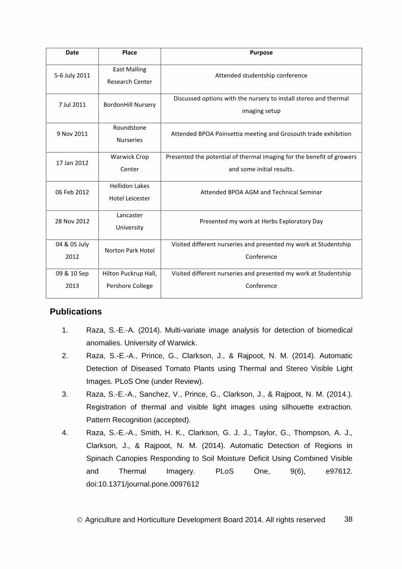
Agriculture and Horticulture Development Board 2014. All rights reserved
38
Date Place Purpose
5-6 July 2011 East Malling
Research Center Attended studentship conference
7 Jul 2011 BordonHill Nursery Discussed options with the nursery to install stereo and thermal
imaging setup
9 Nov 2011 Roundstone
Nurseries Attended BPOA Poinsettia meeting and Grosouth trade exhibition
17 Jan 2012 Warwick Crop
Center
Presented the potential of thermal imaging for the benefit of growers
and some initial results.
06 Feb 2012 Hellidon Lakes
Hotel Leicester Attended BPOA AGM and Technical Seminar
28 Nov 2012 Lancaster
University Presented my work at Herbs Exploratory Day
04 & 05 July
2012 Norton Park Hotel
Visited different nurseries and presented my work at Studentship
Conference
09 & 10 Sep
2013
Hilton Puckrup Hall,
Pershore College
Visited different nurseries and presented my work at Studentship
Conference
Publications
1. Raza, S.-E.-A. (2014). Multi-variate image analysis for detection of biomedical
anomalies. University of Warwick.
2. Raza, S.-E.-A., Prince, G., Clarkson, J., & Rajpoot, N. M. (2014). Automatic
Detection of Diseased Tomato Plants using Thermal and Stereo Visible Light
Images. PLoS One (under Review).
3. Raza, S.-E.-A., Sanchez, V., Prince, G., Clarkson, J., & Rajpoot, N. M. (2014.).
Registration of thermal and visible light images using silhouette extraction.
Pattern Recognition (accepted).
4. Raza, S.-E.-A., Smith, H. K., Clarkson, G. J. J., Taylor, G., Thompson, A. J.,
Clarkson, J., & Rajpoot, N. M. (2014). Automatic Detection of Regions in
Spinach Canopies Responding to Soil Moisture Deficit Using Combined Visible
and Thermal Imagery. PLoS One, 9(6), e97612.
doi:10.1371/journal.pone.0097612
Agriculture and Horticulture Development Board 2014. All rights reserved
39
References
Andersen, H. J., Reng, L., & Kirk, K. (2005). Geometric plant properties by relaxed stereo vision using simulated annealing. Computers and Electronics in Agriculture, 49(2), 219–232. doi:10.1016/j.compag.2005.02.015
Audet, C., & Dennis, J. E. (2002). Analysis of Generalized Pattern Searches. SIAM Journal on Optimization, 13(3), 889. doi:10.1137/S1052623400378742
Belin, É., Rousseau, D., Boureau, T., & Caffier, V. (2013). Thermography versus chlorophyll fluorescence imaging for detection and quantification of apple scab. Computers and Electronics in Agriculture, 90, 159–163. doi:10.1016/j.compag.2012.09.014
Bilodeau, G., St-Onge, P., & Garnier, R. (2011). Silhouette-based features for visible-infrared registration. In Computer Vision and Pattern Recognition Workshop.
Birchfield, S., & Tomasi, C. (1999). Depth discontinuities by pixel-to-pixel stereo. International Journal of Computer Vision, 35(3), 269–293.
Biskup, B., Scharr, H., Schurr, U., & Rascher, U. W. E. (2007). A stereo imaging system for measuring structural parameters of plant canopies. Plant, Cell & Environment, 30(10), 1299–1308. doi:10.1111/j.1365-3040.2007.01702.x
Boykov, Y., & Kolmogorov, V. (2004). An experimental comparison of min-cut/max-flow algorithms for energy minimization in vision. Pattern Analysis and Machine Intelligence, IEEE Transactions on, 26(9), 1124–37. doi:10.1109/TPAMI.2004.60
Boykov, Y., Veksler, O., & Zabih, R. (2001). Fast approximate energy minimization via graph cuts. Pattern Analysis and Machine Intelligence, IEEE Transactions on, 23(11), 1222–1239.
Chaerle, L., Caeneghem, W. Van, & Messens, E. (1999). Presymptomatic visualization of plant-virus interactions by thermography. Nature, 17(8), 813–6.
Chaerle, L., Leinonen, I., Jones, H. G., & Van Der Straeten, D. (2007). Monitoring and screening plant populations with combined thermal and chlorophyll fluorescence imaging. Journal of Experimental Botany, 58(4), 773–84.
Chen, H. M., Lee, S., Rao, R. M., Slamani, M. A., & Varshney, P. K. (2005). Imaging for concealed weapon detection: a tutorial overview of development in imaging sensors and processing. Signal Processing Magazine, IEEE, 22(March 2005), 52–61.
Chen, H., & Varshney, P. (2001). Automatic two-stage IR and MMW image registration algorithm for concealed weapons detection. Vision, Image and Signal Processing, IEEE Proceedings, 148(4), 209–216. doi:10.1049/ip-vis
Chen, S., Su, H., Zhang, R., & Tian, J. (2008). Fusing remote sensing images using à trous wavelet transform and empirical mode decomposition. Pattern Recognition Letters, 29(3), 330–342. doi:10.1016/j.patrec.2007.10.013
Cohen, Y., Alchanatis, V., Prigojin, A., Levi, A., & Soroker, V. (2011). Use of aerial thermal imaging to estimate water status of palm trees. Precision Agriculture, 13(1), 123–140.
Agriculture and Horticulture Development Board 2014. All rights reserved
40
Felzenszwalb, P. F., & Huttenlocher, D. P. (2006). Efficient Belief Propagation for Early Vision. International Journal of Computer Vision, 70(1), 41–54. doi:10.1007/s11263-006-7899-4
Han, J., & Bhanu, B. (2007). Fusion of color and infrared video for moving human detection. Pattern Recognition, 40(6), 1771–1784. doi:10.1016/j.patcog.2006.11.010
Han, J., Pauwels, E. J., & de Zeeuw, P. (2013). Visible and infrared image registration in man-made environments employing hybrid visual features. Pattern Recognition Letters, 34(1), 42–51. doi:10.1016/j.patrec.2012.03.022
Han, J., Pauwels, E., & Zeeuw, P. De. (2012). Visible and infrared image registration employing line-based geometric analysis. Computational Intelligence for Multimedia Understanding, 7252, 114–125.
Hirschmüller, H. (2008). Stereo processing by semiglobal matching and mutual information. Pattern Analysis and Machine Intelligence, IEEE Transactions on, 30(2), 328–41. doi:10.1109/TPAMI.2007.1166
Idso, S. B., Jackson, R. D., Pinter Jr, P. J., Reginato, R. J., & Hatfield, J. L. (1981). Normalizing the stress-degree-day parameter for environmental variability. Agricultural Meteorology, 24(1), 45–55. doi:10.1016/0002-1571(81)90032-7
Ivanov, N., Boissard, P., Chapron, M., & Andrieu, B. (1995). Computer stereo plotting for 3-D reconstruction of a maize canopy. Agricultural and Forest Meteorology, 1923(94).
Jarc, A., Perš, J., Rogelj, P., Perše, M., & Kovacic, S. (2007). Texture features for affine registration of thermal (FLIR) and visible images. Computer Vision WinterWorkshop, 1–7.
Jones, H. G. (2002). Use of infrared thermography for monitoring stomatal closure in the field: application to grapevine. Journal of Experimental Botany, 53(378), 2249–2260. doi:10.1093/jxb/erf083
Ju, X., Nebel, J., & Siebert, J. P. (2004). 3D thermography imaging standardization technique for inflammation diagnosis. In H. Gong, Y. Cai, & J.-P. Chatard (Eds.), Proc. SPIE, Photonics Asia (pp. 266–273). doi:10.1117/12.577055
Kale, K. V. (2008). Advances In Computer Vision And Information Technology. I.K. International Publishing House Pvt. Limited.
Kim, Y. S., Lee, J. H., & Ra, J. B. (2008). Multi-sensor image registration based on intensity and edge orientation information. Pattern Recognition, 41(11), 3356–3365. doi:10.1016/j.patcog.2008.04.017
Kolmogorov, V., & Zabih, R. (2001). Computing visual correspondence with occlusions using graph cuts. Proceedings Ninth IEEE International Conference on Computer Vision, 2, 508–515. doi:10.1109/ICCV.2001.937668
Kolmogorov, V., & Zabih, R. (2002). Multi-camera scene reconstruction via graph cuts. Computer Vision—ECCV 2002.
Kong, S. G., Heo, J., Boughorbel, F., Zheng, Y., Abidi, B. R., Koschan, A., … Abidi, M. a.
Agriculture and Horticulture Development Board 2014. All rights reserved
41
(2006). Multiscale fusion of visible and thermal IR images for illumination-invariant Face Recognition. International Journal of Computer Vision, 71(2), 215–233. doi:10.1007/s11263-006-6655-0
Konolige, K. (1998). Small vision systems: hardware and implementation. Robotics Research International.
Kroon, D.-J. (2011, December 1). Segmentation of the mandibular canal in cone-beam CT data. University of Twente, Enschede, The Netherlands.
Krotosky, S. J., & Trivedi, M. M. (2007). Mutual information based registration of multimodal stereo videos for person tracking. Computer Vision and Image Understanding, 106(2-3), 270–287. doi:10.1016/j.cviu.2006.10.008
Lee, J. H., Kim, Y. S., Lee, D., Kang, D., & Ra, J. B. (2010). Robust CCD and IR image registration using gradient-based statistical information. IEEE Signal Processing Letters, 17(4), 347–350. doi:10.1109/LSP.2010.2040928
Lee, S., Wolberg, G., & Shin, S. Y. (1997). Scattered data interpolation with multilevel B-splines. IEEE Transactions on Visualization and Computer Graphics, 3(3), 228–244. doi:10.1109/2945.620490
Leinonen, I., & Jones, H. G. (2004). Combining thermal and visible imagery for estimating canopy temperature and identifying plant stress. Journal of Experimental Botany, 55(401), 1423–31. doi:10.1093/jxb/erh146
Lenthe, J.-H., Oerke, E.-C., & Dehne, H.-W. (2007). Digital infrared thermography for monitoring canopy health of wheat. Precision Agriculture, 8(1-2), 15–26. doi:10.1007/s11119-006-9025-6
Lindenthal, M., Steiner, U., Dehne, H.-W., & Oerke, E.-C. (2005). Effect of downy mildew development on transpiration of cucumber leaves visualized by digital infrared thermography. Phytopathology, 95(3), 233–40.
Morris, N. J. W., Avidan, S., Matusik, W., & Pfister, H. (2007). Statistics of infrared images. IEEE Conference on Computer Vision and Pattern Recognition, 1–7. doi:10.1109/CVPR.2007.383003
Morse, B. S. (2000). Lecture 11 : Differential Geometry.
Naidu, R. a., Perry, E. M., Pierce, F. J., & Mekuria, T. (2009). The potential of spectral reflectance technique for the detection of Grapevine leafroll-associated virus-3 in two red-berried wine grape cultivars. Computers and Electronics in Agriculture, 66(1), 38–45. doi:10.1016/j.compag.2008.11.007
Nashat, S., Abdullah, A., & Abdullah, M. Z. (2011). A stationary wavelet edge detection algorithm for noisy images (pp. 1–9).
Nason, G., & Silverman, B. (1995). The stationary wavelet transform and some statistical applications. Wavelets and Statistics, 1–19.
Oerke, E.-C., Fröhling, P., & Steiner, U. (2011). Thermographic assessment of scab disease on apple leaves. Precision Agriculture, 12(5), 699–715. doi:10.1007/s11119-
Agriculture and Horticulture Development Board 2014. All rights reserved
42
010-9212-3
Oerke, E.-C., Gerhards, R., & Menz, G. (2010). Precision Crop Protection - the Challenge and Use of Heterogeneity (p. 441). Springer.
Oerke, E.-C., & Steiner, U. (2010). Potential of digital thermography for disease control. In Precision Crop Protection—the Challenge and use of Heterogeneity (pp. 167–182). Dordrecht, Netherlands: Springer Netherlands.
Oerke, E.-C., Steiner, U., Dehne, H.-W., & Lindenthal, M. (2006). Thermal imaging of cucumber leaves affected by downy mildew and environmental conditions. Journal of Experimental Botany, 57(9), 2121–32. doi:10.1093/jxb/erj170
Olivo-Marin, J.-C. (2002). Extraction of spots in biological images using multiscale products. Pattern Recognition, 35(9), 1989–1996. doi:10.1016/S0031-3203(01)00127-3
Omasa, K., Hosoi, F., & Konishi, A. (2007). 3D lidar imaging for detecting and understanding plant responses and canopy structure. Journal of Experimental Botany, 58(4), 881–98. doi:10.1093/jxb/erl142
Pajares, G., & Manuel de la Cruz, J. (2004). A wavelet-based image fusion tutorial. Pattern Recognition, 37(9), 1855–1872. doi:10.1016/j.patcog.2004.03.010
Perona, P., & Malik, J. (1990). Scale-space and edge detection using anisotropic diffusion. IEEE Transactions on Pattern Analysis and Machine Intelligence, 12(7), 629–639.
Pluim, J. P. W., Maintz, J. B. A., & Viergever, M. A. (2003). Mutual-information-based registration of medical images: a survey. IEEE Transactions on Medical Imaging, 22(8), 986–1004. doi:10.1109/TMI.2003.815867
Raza, S.-E.-A., Smith, H. K., Clarkson, G. J. J., Taylor, G., Thompson, A. J., Clarkson, J., & Rajpoot, N. M. (2014). Automatic Detection of Regions in Spinach Canopies Responding to Soil Moisture Deficit Using Combined Visible and Thermal Imagery. PloS One, 9(6), e97612. doi:10.1371/journal.pone.0097612
Rosell, J. R., & Sanz, R. (2012). A review of methods and applications of the geometric characterization of tree crops in agricultural activities. Computers and Electronics in Agriculture, 81, 124–141. doi:10.1016/j.compag.2011.09.007
Rueckert, D., Sonoda, L. I., Hayes, C., Hill, D. L., Leach, M. O., & Hawkes, D. J. (1999). Nonrigid registration using free-form deformations: application to breast MR images. IEEE Transactions on Medical Imaging, 18(8), 712–21. doi:10.1109/42.796284
Scharstein, D., & Szeliski, R. (2002). A taxonomy and evaluation of dense two-frame stereo correspondence algorithms. International Journal of Computer Vision, 47(1), 7–42. doi:10.1023/A:1014573219977
Song, Y., Wilson, R., Edmondson, R., & Parsons, N. (2007). Surface modelling of plants from stereo images. In Sixth International Conference on 3-D Digital Imaging and Modeling (3DIM 2007) (pp. 312–319). IEEE.
Stoll, M., & Jones, H. (2007). Thermal imaging as a viable tool for monitoring plant stress. International Journal of Vine and Wine Sciences, 41(2), 77–84.
Agriculture and Horticulture Development Board 2014. All rights reserved
43
Stoll, M., Schultz, H. R., & Berkelmann-Loehnertz, B. (2008). Thermal sensitivity of grapevine leaves affected by Plasmopara viticola and water stress. Vitis-Geilweilerhof, 47(2), 133.
Sun, H., Wei, J., Zhang, J., & Yang, W. (2014). A comparison of disease severity measurements using image analysis and visual estimates using a category scale for genetic analysis of resistance to bacterial spot in tomato. European Journal of Plant Pathology, 139(1), 125–136. doi:10.1007/s10658-013-0371-8
Torabi, A., & Bilodeau, G.-A. (2013). Local self-similarity-based registration of human ROIs in pairs of stereo thermal-visible videos. Pattern Recognition, 46(2), 578–589. doi:10.1016/j.patcog.2012.07.026
Torabi, A., Massé, G., & Bilodeau, G.-A. (2012). An iterative integrated framework for thermal–visible image registration, sensor fusion, and people tracking for video surveillance applications. Computer Vision and Image Understanding, 116(2), 210–221. doi:10.1016/j.cviu.2011.10.006
Verstockt, S., Poppe, C., Van Hoecke, S., Hollemeersch, C., Merci, B., Sette, B., … Van de Walle, R. (2011). Silhouette-based multi-sensor smoke detection. Machine Vision and Applications, 23(6), 1243–1262. doi:10.1007/s00138-011-0359-3
Yang, Q. (2012). A non-local cost aggregation method for stereo matching. IEEE Conference on Computer Vision and Pattern Recognition, 1402–1409. doi:10.1109/CVPR.2012.6247827
Yang, Q., Wang, L., & Ahuja, N. (2010). A constant-space belief propagation algorithm for stereo matching. Computer Vision and Pattern Recognition (CVPR), IEEE Conference on, 1458–1465. doi:10.1109/CVPR.2010.5539797
Zhao, J., & Cheung, S. S. (2012). Human segmentation by geometrically fusing visible-light and thermal imageries. Multimedia Tools and Applications. doi:10.1007/s11042-012-1299-2
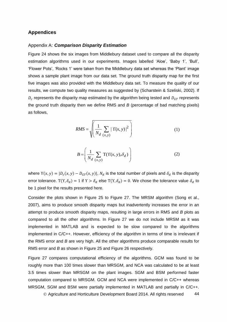
Agriculture and Horticulture Development Board 2014. All rights reserved
44
Appendices
Comparison Disparity Estimation Appendix A:
Figure 24 shows the six images from Middlebury dataset used to compare all the disparity
estimation algorithms used in our experiments. Images labelled ‘Aloe’, ‘Baby 1’, ‘Bull’,
‘Flower Pots’, ‘Rocks 1’ were taken from the Middlebury data set whereas the ‘Plant’ image
shows a sample plant image from our data set. The ground truth disparity map for the first
five images was also provided with the Middlebury data set. To measure the quality of our
results, we compute two quality measures as suggested by (Scharstein & Szeliski, 2002). If
represents the disparity map estimated by the algorithm being tested and represents
the ground truth disparity then we define RMS and B (percentage of bad matching pixels)
as follows,
2
( , )
1| ( , ) |
d x y
RMS x yN
(1)
( , )
1T( ( , ), )d
d x y
B x yN
(2)
where , is the total number of pixels and is the disparity
error tolerance. if else . We chose the tolerance value to
be 1 pixel for the results presented here.
Consider the plots shown in Figure 25 to Figure 27. The MRSM algorithm (Song et al.,
2007), aims to produce smooth disparity maps but inadvertently increases the error in an
attempt to produce smooth disparity maps, resulting in large errors in RMS and B plots as
compared to all the other algorithms. In Figure 27 we do not include MRSM as it was
implemented in MATLAB and is expected to be slow compared to the algorithms
implemented in C/C++. However, efficiency of the algorithm in terms of time is irrelevant if
the RMS error and B are very high. All the other algorithms produce comparable results for
RMS error and B as shown in Figure 25 and Figure 26 respectively.
Figure 27 compares computational efficiency of the algorithms. GCM was found to be
roughly more than 100 times slower than MRSGM, and NCA was calculated to be at least
3.5 times slower than MRSGM on the plant images. SGM and BSM performed faster
computation compared to MRSGM. GCM and NCA were implemented in C/C++ whereas
MRSGM, SGM and BSM were partially implemented in MATLAB and partially in C/C++.
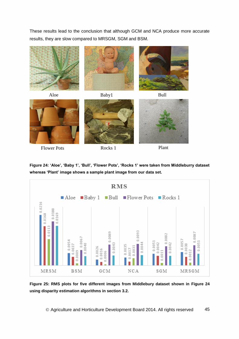
Agriculture and Horticulture Development Board 2014. All rights reserved
45
These results lead to the conclusion that although GCM and NCA produce more accurate
results, they are slow compared to MRSGM, SGM and BSM.
Figure 24: ‘Aloe’, ‘Baby 1’, ‘Bull’, ‘Flower Pots’, ‘Rocks 1’ were taken from Middleburry dataset
whereas ‘Plant’ image shows a sample plant image from our data set.
Figure 25: RMS plots for five different images from Middlebury dataset shown in Figure 24
using disparity estimation algorithms in section 3.2.
Aloe Baby1 Bull
Flower Pots Rocks 1 Plant
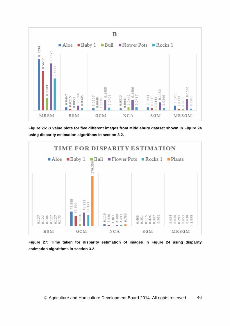
Agriculture and Horticulture Development Board 2014. All rights reserved
46
Figure 26: B value plots for five different images from Middlebury dataset shown in Figure 24
using disparity estimation algorithms in section 3.2.
Figure 27: Time taken for disparity estimation of images in Figure 24 using disparity
estimation algorithms in section 3.2.