March 2021

Project Report No. 629

Integrated platforms for barley breeding and genetic researchJoanne Russell, Robbie Waugh, Kelly Houston and Helena Oakey

The James Hutton Institute,

Invergowrie, Dundee DD2 5NE

This is the final report of a 12-month project (21130015) that started in April 2016. The work was funded by contract for £58,271 from AHDB.

While the Agriculture and Horticulture Development Board seeks to ensure that the information contained within this document is

accurate at the time of printing, no warranty is given in respect thereof and, to the maximum extent permitted by law, the Agriculture and

Horticulture Development Board accepts no liability for loss, damage or injury howsoever caused (including that caused by negligence)

or suffered directly or indirectly in relation to information and opinions contained in or omitted from this document.

Reference herein to trade names and proprietary products without stating that they are protected does not imply that they may be

regarded as unprotected and thus free for general use. No endorsement of named products is intended, nor is any criticism implied of

other alternative, but unnamed, products.

AHDB Cereals & Oilseeds is a part of the Agriculture and Horticulture Development Board (AHDB).

CONTENTS

1. ABSTRACT ........................................................................................................................... 1

2. INTRODUCTION ................................................................................................................... 2

3. MATERIALS AND METHODS .............................................................................................. 3

3.1. Phenotypic Data ....................................................................................................... 3

3.2. Genotypic Data ......................................................................................................... 3

3.3. Population Structure ................................................................................................ 4

3.4. Diversity for seasonal growth habit and ear row number ..................................... 4

3.5. Genome Wide Association Mapping ....................................................................... 5

3.6. KASP marker sequence identification .................................................................... 6

4. RESULTS .............................................................................................................................. 6

4.1. Population Structure ................................................................................................ 6

4.2. Diversity for seasonal growth habit and ear row number ..................................... 8

4.3. Genome Wide Association Mapping ..................................................................... 13

4.4. Other DUS traits ..................................................................................................... 18

4.5. KASP marker sequence identification .................................................................. 21

5. DISCUSSION ...................................................................................................................... 22

6. REFERENCES .................................................................................................................... 24

7. SUPPLEMENTARY 1 .......................................................................................................... 27

8. SUPPLEMENTARY 3 .......................................................................................................... 33

9. SUPPLEMENTARY 4 .......................................................................................................... 38

9.1. Supplementary 5.................................................................................................... 45

1

1. Abstract

This project aimed to discover new molecular diagnostics for use in barley breeding programmes.

It exploited phenotypic data and high-density genetic marker data, generated by resequencing the

germplasm assembled under the Association genetics of UK elite barley – AGOUEB project

(AHDB Project Report 528). In AGOUEB, we assembled a vast collection of new and legacy

phenotypic data and conducted preliminary genetic analyses. However, the initial AGOUEB work

was of relatively low resolution (c. 1000 markers). As a result, the project lacked the highest level

of informativeness. Additionally, most of the phenotypic data was not analysed optimally and

remained unpublished.

This project had the following objectives:

1. To use a new high-density genetic marker dataset (c. 2,100,000 SNP markers) to analyse

phenotypic data initially assembled and analysed in AGOUEB.

2. To discover and provide the information required to convert diagnostic markers into

breeder-friendly marker systems.

3. To publicise findings to the scientific and end-user communities.

Reanalysis of the phenotypic dataset, with the new high density marker set, represented a greater

than 130 fold increase in genetic marker density. This allowed us to define genomic regions that

contain genes responsible for 31 traits. We were also able to identify SNPs that are significantly

associated with each of these traits. For each of these SNPs, putative sequences for KASP

markers have been identified. We are pursuing serveral of these traits, with various collaborators,

with the view to identify and characterise the casual genes.

The progress made in AGOUEB and this project marks a significant step forward in the ability to

better track key barley traits through breeding programmes.

2

2. Introduction

Advances in the assembly of DNA sequence data of barley means that it is now possible to

compare variation amongst different barley lines across some 60,000 sequences representing

barley genes. Previous work under the AGOUEB project had assessed AHDB Recommended List

and National List data to identify markers associated with agronomic, yield, quality and DUS data.

But, as only ~ 1000 SNPs were available at the time, the resolution was insufficient to resolve the

differences down to potential candidate genes based purely on these markers (Cockram et al

2010). This last step is essential for effective and rapid mining of gene-bank collections for future

improvements in breeding. Therefore, the main focus of the INTEGRA project has been the re-

analysis of the AGOUEB data sets with the new SNP data revealed from the analysis of the data

generated from exome capture sequences to test whether we can identify candidate genes for

some of the un-resolved DUS traits characters.

The aim of this project is to rapidly exploit data from newly assembled genetic marker information

to analyse phenotypic data collected – but, so far not optimally analysed – in a previous HGCA

sponsored project. Analysis of the trait data with the new marker data will increase our ability to

genetically resolve regions of the barley genome that control economically important traits, and

then facilitate facile marker assisted selection in commercial plant breeding programmes. The

project takes advantage of recent barley genomic research outcomes (IBSC 2012, Mascher et al

2013) and commercial technologies such as KASP and Affymetrix genotyping to generate a

platform for genetic analysis in this crop.

The ability to monitor the inheritance of segments of the genome using ‘genetic markers’ in simple

and complex populations is the core of modern genetics. Only 25 years ago, as few as tens or

hundreds of markers were assayed in plant genetic studies, often through laborious techniques

that involved the use of radioactivity (Beckmann and Soller 1983, Vos et al 1995). Today, as the

result of a series of intricate and innovative technological developments, millions of markers can

now be followed in a single experiment (Clark et al 2007) both quickly and at relatively low cost.

For these 25 years, we have been at the forefront of genetic marker technology development and

implementation in cultivated barley (Waugh et al 1997, Ramsay et al 2000, Close et al 2009). The

most accessible and widely used resource currently available is an Illumina iSelect platform that

assays genetic variation at 9000 sites across the genome that contain single nucleotide

polymorphisms (SNPs) (Comadran et al 2012) While this platform has been an exceptionally

powerful tool for genetic studies, it suffers from a combination of ascertainment bias (Moragues et

al 2010), relatively high cost, and, due to marker numbers, and the inability to adequately exploit all

of the recombination events (genetic power) present in experimental populations.

3

In INTEGRA-2.1 we plan to exploit a very high density 2.1M SNP dataset collected by

resequencing the AGOUEB germplasm to analyse the phenotypic data that we collected in the

AGOUEB and related programmes. This should provide unprecedented power to detect

associations between molecular markers and phenotypic traits that can subsequently be deployed

in accelerating genetic gain in plant breeding. Our analyses will provide many new leads (genes)

and supporting information for several end-user relevant projects, facilitating the development of

molecular diagnostics and enabling trait gene discovery.

The exome capture sequencing platform is relatively expensive and not routine in a breeding

situation. To make the data more widely applicable, we are using 58,000 of the most robust and

informative SNPs discovered using this approach to develop a generic genotyping platform for

release to the broader community, through collaboration with the commercial organisation

Affymetrix. This platform will provide a >97.5% reduction in cost per informative SNP datapoint

over current technologies, making it financially accessible to entire communities.

The objectives of this project are below:

1. To use a new very high density genetic marker dataset (ca. 2,100,000 SNP markers) to analyse

phenotypic data first assembled and analysed in a previous HGCA sponsored project - AGOUEB.

2. To discover and provide the information required to convert diagnostic markers into breeder-

friendly marker systems

3. To publicise our findings to the relevant scientific and end-user communities

3. Materials and methods

3.1. Phenotypic Data

We have re-investigated a total of 32 DUS traits which were analysed previously by Cockram et al.

(2010) having been scored in ~500 lines which were genotyped using the bOPA1 genotyping

platform which consisted of 1536 SNPs. For two of the DUS traits, seasonal growth habit (spring

or winter) and ear row number (2 or 6) we have 357 lines that have both phenotypic and genotypic

data derived from exome capture. For the other 30 DUS traits, the number of lines with both

phenotypic and genotypic data for the DUS traits varies from 159 to 179 depending on the trait.

3.2. Genotypic Data

A total of 138545 SNPs from exome capture were available for up to 357 lines from the BBSRC UK

barley genome project (unpublished). These SNPs had passed the following filtering criteria:

1. >= 8x coverage for >= 50% of the samples (to ensure robust SNP and genotype calls)

2. >= 95% of samples represented at SNP locus (for maximum sample representation)

4

3. >= 5% minor allele frequency at the level of the sample, i.e., counting sample genotypes rather than individual reads (to exclude SNPs based on very rare alleles) 4. >= 30 SNP quality score, equating to a >= 1/1000 chance of the SNP having been called in error (for SNP robustness) 5. >= 98% of samples homozygous (to reduce false positives by removing variants that are the result of read mis-mapping or Illumina systematic sequencing error) 6. no indels Missing SNP values were imputed for each chromosome separately using the R packages linkim

(Xu and Wu, 2014) after recoding the SNP alleles 0 and 1.

3.3. Population Structure

The population structure of the initial 357 lines was investigated using Principal Component

Analysis performed in R version 3.2.4 (R core Team, 2016).

3.4. Diversity for seasonal growth habit and ear row number

There were 357 lines characterised for seasonal growth habit (spring or winter) and ear row

number (2 or 6) and for spring lines and whether it was exotic (exotic or non-exotic).

The divergency of the lines within different populations was investigated using the fixation indexes

ΦST (Meirmans 2006), which is a locus-by-locus estimate of population diversity (defined as a

function of the between population variance component and the within variance component)

comparing the between population genetic variance to the total genetic variation over all

populations and GST (Nei 1973) which is the locus-by-locus estimates of expected heterozygosity

(gene diversity) between populations compared to the total genetic diversity. The fixation indexes

range from zero which indicates no differentiation between the overall population and its

subpopulations to a theoretical maximum of one. Negative values can be obtained (Meirmans

2006) and these can be interpreted as no population structure being present and are reset to a

value of zero.

Where numbers allowed, further subpopulations were investigated (Table 1), Spring with ear row

number two verses Spring with ear row number six, Winter with ear row number two verses Winter

with ear row number six and Spring with ear row number two verse Winter with ear row number

two. The number of SNP markers available for the comparison of these smaller populations

reduces from the maximum of 138,545 as some of the SNPs become monomorphic with the

smaller number of lines within the subpopulation comparisons.

Table 1: Number of lines in each subgroup Ear Row Number Total

Seasonal growth habit 2 6

Spring 230 29 259

Winter 70 28 98

300 57 357

5

The library mmod (Winter 2012) within R version 3.2.4 (R core Team, 2016) was used to calculate

the fixation indexes ΦST (Meirmans 2006) and GST (Nei 1973). Manhattan plots were used to show

the minus inverse of the fixation indexes and created in using the R library qqman (Turner 2014).

3.5. Genome Wide Association Mapping

For each DUS trait with more than two responses (Supplementary S4), the association analysis

fitted was a linear mixed model:

𝒚𝒚 = 𝑿𝑿𝑿𝑿 + 𝒁𝒁𝒁𝒁 + 𝒆𝒆

where 𝒚𝒚 is the vector of the mean response for each of 𝑛𝑛 lines, 𝑿𝑿 is a vector of fixed covariate

terms consisting of an overall intercept term, the marker covariate and principal components, 𝑿𝑿 is

the associated design matrix, 𝒁𝒁~𝑁𝑁(0,𝜎𝜎𝑔𝑔2𝑲𝑲) is the vector of random line effects with kinship matrix

𝑲𝑲 representing relationships between lines which was generated by the method of VanRaden

(2008) with design matrix 𝒁𝒁, 𝒆𝒆~𝑁𝑁(0,𝜎𝜎2𝑰𝑰) is the residual effect, where 𝑰𝑰 is the identity matrix. A

separate model is fitted for each SNP marker. The marker effect represents the additive difference

between the two homozygous individuals with opposing SNP alleles. The number of principal

components included in the model was three and was chosen to reflect the structure in the

population corresponding to season growth habit and row type. The kinship matrix (VanRaden

2008) and PCA components for analysis were created in GAPIT (Lipka et al 2012) for consistency

and each model was run in GAPIT.

For the binomial DUS traits with two responses (Table 2), we fitted a generalised linear mixed

model (GLMM).

𝜼𝜼 = 𝑔𝑔(𝐸𝐸(𝒚𝒚|𝑿𝑿,𝒁𝒁)) = 𝑔𝑔(𝜋𝜋) =log� 𝜋𝜋1−𝜋𝜋

� = 𝑿𝑿𝑿𝑿+ 𝒁𝒁𝒁𝒁

Where 𝜼𝜼 is the linear predictor, 𝑔𝑔 is the logit link function, 𝒚𝒚 is the vector of responses with

Bernoulli distribution, 𝜋𝜋 is the unknown probability of response B (Table 2), 1 − 𝜋𝜋 is the probability

of response A; 𝑿𝑿 is vector of fixed covariate terms, consisting of an intercept term, covariate terms

for principal components and the SNP marker, 𝒁𝒁~𝑁𝑁(0,𝑲𝑲) is a random term for lines where 𝑲𝑲 is the

kinship matrix.

The significance of the fixed marker term is assessed using a Walds test, which is compared to an

asymptotic chi-squared distribution.

The GLMM models were fitted using the library ASReml (Butler et al 2009) within R version 3.2.4

(R core Team, 2016). ASReml uses a penalised quasi-likelihood technique based on a first order

Taylor series approximation to the likelihood. The kinship matrix (VanRaden 2008) and PCA

components used in the GLMM were created in GAPIT (Lipka et al 2012).

6

Table 2: Binomial DUS Trait Summary

3.6. KASP marker sequence identification

After identifying the SNP with the most significant association for each trait included in the analysis,

we referred back to the exome capture dataset to identify a sequence that would facilitate the

conversion of this SNP into a KASP genotyping marker. In addition to identifying 100 nucleotides

either side of the SNP (LGC Biosciences requirement is at least 50 nucleotides either side of the

SNP) due to the available exome capture data, we were able to annotate SNPs that were variable

between lines in this dataset with the appropriate IUPAC nucleotide code. Therefore, we have at

least one sequence per trait available for KASP assay.

4. Results

4.1. Population Structure

The initial population of 357 lines was investigated for genetic substructure using principal

components analysis on the 138,545 SNPs. The first three principal components account for

18.4% of the variance in the population and distinguish between the phenotypic combinations of

row number and seasonal growth habit.

Binomial DUS Trait Response A (Number of lines)

Response B (Number of lines)

Total Number of lines

Awn anthocyanin colouration of tips Present (127) Absent (32) 159

Awn spiculation of margins Reduced (1) Present (137) 138

Flag leaf anthocyanin colouration of auricle Present (117) Absent (30) 147

Grain disposition of lodicules Frontal (3) Clasping (158) 161

Grain husk Present (160) Absent (3) 163

Grain rachilla hair type Short (36) Long (143) 179

Grain ventral furrow presence of hairs Present (31) Absent (145) 176

Lower leaf hairiness of leaf sheaths Present (66) Absent (109) 175

7

S2=Spring 2 row, S6=spring 6 row, W2=Winter 2 row, W6=winter row

8

4.2. Diversity for seasonal growth habit and ear row number

Both seasonal growth habit and row type are also binomial variables, and as such, we attempted to

fit a binomial GWAS model to the data. This brought problems related to the population structure of

the data set. In GWAS, the principal components are included in the model to account for any

population structure. However, as illustrated in the previous section, the population structure in this

data set reflects both the seasonal growth habit and the row type - the two traits that we are

interested in. Thus, in the initial binomial GWAS models fitted, the principal components

9

accounted for all the genetic variation due to seasonal growth habit and row type. Therefore, we

failed to identify any significant SNP markers which distinguished between the winter and spring or

2 row and 6 row. Conversely, failing to include the principal components in the model resulted in

over 21,000 SNP markers with a –log10(pvalue) greater than 10. With so many significant SNP

markers it is clearly impossible to distinguish ‘real’ significance from a false-positive. For this

reason, we decided to investigate the seasonal growth habit and the row type using fixation

indices.

There were 357 lines characterised for seasonal growth habit (spring or winter) and ear row

number (2 or 6) for which there was a total of 138,545 SNPs from exome capture that were

included in the fixation index analysis.

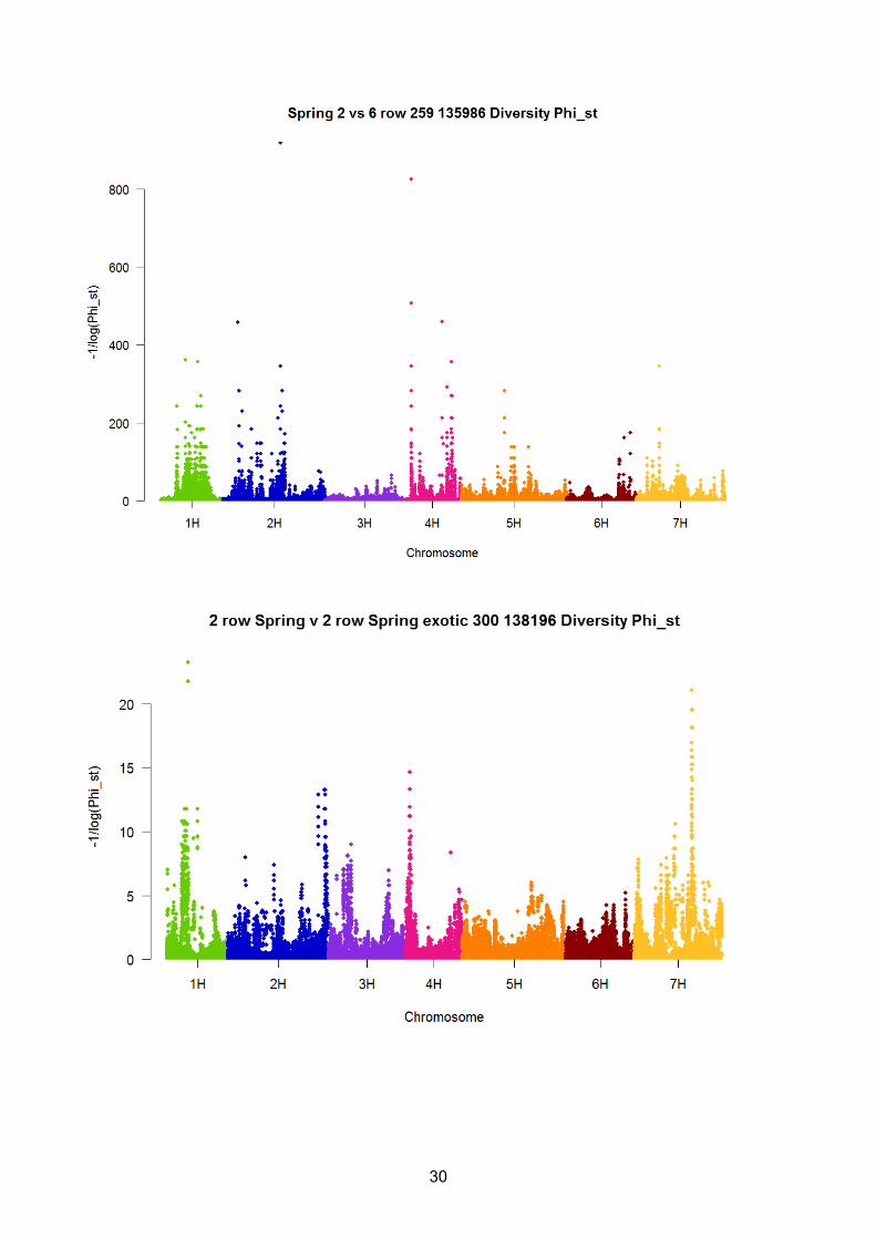
Plots of minus the inverse of the fixations index GST (Nei 1973) are shown in Figures 1 to 6, with

plots of the fixation index ΦST (Meirmans 2006) shown in the supplementary material (S1). For the

most part, the SNPs identified as defining the diversity between the studied populations were the

same under both indexes. In cases where they differed, the SNPs were in the same genomic

region. For Spring 2 vs 6 row, the ΦST fixation index identified a potential SNP at 7H which was not

as obvious from the GST index, however, this SNP had a diversity value at least half as small as the

most important SNPs on 2H.

The results for 6 row Spring vs Winter are not shown. There were a small number of lines in this

group (57) with only 29 possible different allele frequencies within the 131,139 SNPs available and

therefore, a limited number of possible fixation index values. For spring lines, we also had details

of which were exotic lines and a comparison within spring lines was made, these are shown in

Figure 6.

The regions identified using this analysis on the complete set of 357 lines for row type highlighted a

region on 4HS that was strongly divergent for this trait, along with other regions on 1H, 2H and 4H

being of potential interest (Figure 2). These overlapped with regions of the genome identified

before for this agronomically important, and therefore, a well-studied trait, but both validate use of

this approach for identifying regions important for traits in populations not suited to GWAS and

provide opportunities to design markers specific to this germplasm. Previously, 5 Vrs loci have

been indicated as regulating row type and located on 1HS (Vrs3), 2HL (Vrs1), 3HS (Vrs4), 4HS

(Vrs5), and 5HL (Vrs2), and in the case of all loci except for Vrs3 the causal gene has been

published (Komatsdua et al 2007, Ramsay et al., 2011, Koppulu et al 2013, and Youssef et al.,

2016). Several additional regions of the genome to those described above were highlighted in our

analysis.

Similarly, for another important and well-studied trait, seasonal growth habit, several regions were

identified as being divergent in our analysis (Figure 1) which had been previously identified

contributing to this trait (summarised in Hill and Li 2016).

10

Figure 1

Figure 2

11

Figure 3

12

Figure 4

Figure 5

13

Figure 6

4.3. Genome Wide Association Mapping

4.3.1. Binomial DUS traits

In total, seven DUS traits were analysed using a binomial model. Initially, all the models for all traits

were fitted including three principal components. However, we found that for the binomial DUS trait

GWAS, model convergence was sensitive to the number of principal components included.

Additionally, not all principal components were found to be significant. Therefore, to improve

convergence, for five of the binomial DUS traits, we reduced the number of principal components

included in the final GWAS model if they were not significant from three to either two or one (Table

3). It should be noted that the results were not materially changed by altering the number of

principal components, but the convergence of the model improved.

14

Table 3: Final number of principal components included in the GWAS for each Binomial DUS trait

Binomial DUS Trait Number of principal components included in the final model

Number of models not converged

Awn anthocyanin colouration of tips 2 1

Flag leaf anthocyanin colouration of auricle 2 1

Grain disposition of lodicules 3 1527

Grain husk 2 702

Grain rachilla hair type 3 0

Grain ventral furrow presence of hairs 1 0

Lower leaf hairiness of leaf sheaths 1 3014

Figures 7 - 10 show Manhattan plots of the –log10(pvalue) results (of converged models only) for

responses where a clear peak is shown and include Awn anthocyanin colouration of tips, Flag leaf

anthocyanin colouration of auricle, Grain ventral furrow presence of hairs and Grain rachilla hair,

respectively. Significant SNPs have been identified and these are shown in Figures 7 – 10.

Results for other binomial DUS traits, except Awn spiculation of margins, are shown in

Supplementary material (S2). These latter DUS traits include Grain disposition of lodicules, Lower

leaf hairiness of leaf sheaths and Grain husk where no peaks of any significance are shown for

converged models. Grain disposition of lodicules has only 3 lines (Dew, Felicie and Prisma)

representing the frontal group and Grain husk had only 3 lines (Cassata, Carola and Penthouse)

representing the absent group so that the results from these variables should be treated with

caution. The DUS traits Awn spiculation of margins had only one line representing the reduced

category and no lines representing the absent category and therefore, this variable was not

analysed.

We examined the SNP models which failed to converge to try and identify reasons for non-

convergence. We found the reason for non-convergence could be explained by the distribution of

counts across the trait and marker by cells with very low counts. For instance, the GWAS model for

a SNP marker on chromosome 1 failed to converge for Lower leaf hairiness of leaf sheaths. When

we examine the 2x2 table for trait and marker, we can see cells within the table with low counts.

15

Leaf sheaf Hair

Marker Present Absent

0 1 157

1 0 3

In a simple Chi-square calculation, cells with low counts cause issues with the calculation of

pvalues. In the case of the binomial model, it makes estimation of components difficult and thus,

convergence is compromised. In the case of lower leaf hairiness of leaf sheaths, none of the

unconverged results would have resulted in significant SNP marker p-values.

However, for the Grain disposition of lodicule trait, the non-convergent may represent SNPs would

have otherwise been significant had convergence been achieved. For example, a SNP on

chromosome 2H has a 2x2 table as follows:

Grain lodicule

Marker Frontal Clasping

0 158 0

1 0 3

This SNP had a –log10(pvalue) of 4.45 estimated from the unconverged model. For this reason,

figures for variables with unconverged models (Table 3), are provided (Supplementary 3) which

also include the results of the unconverged models. However, these results should be treated with

caution as in the case of the grain disposition of lodicules the significance of the non-converged

model has to be weighed with the fact that there are only 3 varieties in the clasping response

group.

Results from the INTEGRA analysis corroborated Cockram et al (2010). Like this previously

published study we identified HvbHLH1 as underlying anthocyanin pigmentation in several tissues

(Figure 7 and 8). The increased marker density and therefore, improved resolution of the

association mapping carried out as part of INTEGRA provides opportunities to identify markers

linked to other DUS traits, for example, grain ventral furrow hair (Figure 9), and grain rachilla hair

type (Figure 10). The results from grain rachilla hair which has a significant peak on 5H have been

passed onto colleagues from the JHI who will pursue the identification of causal genes further.

16

Figure 7

Figure 8

17

Figure 9

Figure 10

18

It is worth noting that the interpretation of marker effects in a binomial model is different from a

standard association mapping model and is explained briefly as follows using an example. A

marker on chromosome 5H has the marker effect of 6.49 for grain rachilla hair, thus, for this

marker characterised by the C and T allele, a change in genotype from CC to TT INCREASES the

odds of having long rachilla hair by 658.6 or 65,760%. (Note: genotypes CC and TT are

represented as 0 and 1 in the SNP file and therefore, an increase in 1 unit represents the

difference between the two homozygotes). Conversely, an alternative marker characterised by the

A and T allele on chromosome 5H has a marker effect of -6.36 for grain rachilla hair, so a change

in genotype from AA to TT DECREASES the odds of the long grain hair by 0.002 or 99.82%.

4.4. Other DUS traits

As expected, associations for all traits analysed were found in the same genomic regions when

comparing to Cockram et al. (2010).

Figures 11 to 15 show –log10(p value) results for traits where a clear peak is shown and include

Awn anthocyanin intensity of colouration of tips, Flag leaf anthocyanin intensity of colouration of

auricle, Grain anthocyanin colouration of lemma nerves, grain speculation of inner later nerves and

kernel colour of aleurone, respectively. The ~130 fold increase in marker density clearly provides

an improvement in resolution, and more robust markers. Significant SNPs are clearly evident in

Figures 11 – 15. We identified a strong association for the aleurone trait on 4H (Figure 15). It is the

intention to further pursue the causal gene for aleurone layer colour, also known as blue aleurone,

in collaboration with Ryan Whitford at the University of Adelaide. Aleurone colour can be

considered a “quality trait with a preference for white aleurone. This preference can lead to the

rejection of grain by barley buyers, for instance in Western Australia typically all blue aleurone

grain is turned down (https://www.agric.wa.gov.au/barley/barley-blue-aleurone).

Results for other DUS traits are shown in Supplementary material (S5). These latter DUS traits

include Awn length compared to ear, collar type, ear attitude, ear density, ear glaucosity, ear

length, ear shape, flag leaf glaucosity, medium spikelet length of glume awn, plant frequency of

recurved leaves, growth habit, plant length, rachis curvature, rachis length, sterile spikelet attitude,

sterile spikelet shape and time of ear emergence.

The ear glaucosity has evidence of a peak on 1H which is of interest to colleagues who will pursue

the identification of causal genes further.

19

Figure 11

Figure 12

20

Figure 13

Figure 14

21

Figure 15

4.5. KASP marker sequence identification

One of the objectives of this project was to identify putative markers for the traits analysed and

convert them into a format that can be used in plant breeding programs. From our analysis we

identified associations for 25 traits with a LOD value of greater than the arbitrary threshold of LOD

=3.0. However, we prefer to use the FDR (false discovery rate) threshold (q<0.05), and in this

case, 12 of the characteristics analysed passed this threshold. Combining the outputs from the

GWAS with the genotypic data from the most significant SNPs for these traits has allowed us to

calculate the reliability of these markers based on the accessions used in the GWAS analysis, and

the occurrence of mismatch between genotype and phenotype at each putative marker (data not

shown).

As mentioned in section 4.3.1, for traits such as Awn spiculation of margins, Grain disposition of

lodicules, Lower leaf hairiness of leaf sheaths and Grain husk there was issues with the analysis.

For Awn spiculation of margins there was only one line representing the reduced category and no

lines representing the absent category, and for the same reason the analysis of the other 3 traits

did not identify QTLs that were considered appropriate for marker development.

22

Table 4: Traits which we have identified significant associations, and therefore, have sequences available for the development of KASP genotyping markers.

5. Discussion

During this project we combined high density genetic data derived from exome capture with

phenotypic data to identify and refine key regions of the barley genome for a collection of DUS

traits. In the majority of cases, our analysis identified the same QTL’s as Cockram et al (2010).

However, in the current analysis we extended our analysis to account for the binomial distribution

of several of these DUS traits, Awn anthocyanin colouration of tips, Flag leaf anthocyanin

colouration of auricle, Grain disposition of lodicules, Grain husk, Grain rachilla hair type, Grain

ventral furrow presence of hairs, and Lower leaf hairiness of leaf sheaths. As expected, applying a

generalised linear mixed model (GLMM) to account for the binomial distribution of these traits the

LOD values were lower compared to those when we used the standard model in GAPIT (Genome

Association and Prediction Integrated Tool), but not necessarily lower than those identified in

Cockram et al., (2010) due to different SNPs being present in the respective marker sets.

A second extension of the analysis in the current project was that to determine the efficiency of our

analysis approach in removing loci contributing to variation in row type and Winter/ Spring growth

habit. We exploited these differences using a diversity statistic analogous to FST known as GST.

This revealed multiple loci already known to contribute to these traits, for example, in the case of

Trait - pass FDR (q<0.05) Trait - LOD> 3.0AWN SPICULATION OF MARGINS AWN SPICULATION OF MARGINS AWNS ANTHOCYANIN COLOURATION OF TIPS AWNS ANTHOCYANIN COLOURATION OF TIPS AWNS INTENSITY OF ANTHOCYANIN COLOUR OF AWN TIPS AWNS INTENSITY OF ANTHOCYANIN COLOUR OF AWN TIPS EAR NUMBER OF ROWS COLLAR TYPE FLAG LEAF ANTHOCYANIN COLOURATION OF AURICLES EAR ATTITUDE at least 21 days after ear emerg FLAG LEAF GLAUCOSITY OF SHEATH EAR DENSITY GRAIN ANTHOCYANIN COLOURATION OF LEMMA NERVES EAR GLAUCOSITY GRAIN DISPOSITION OF LODICULES EAR LENGTH EXCLUDING AWNS GRAIN HUSK EAR NUMBER OF ROWS GRAIN RACHILLA HAIR TYPE EAR SHAPE GRAIN SPICULATION OF INNER LATERAL NERVES FLAG LEAF ANTHOCYANIN COLOURATION OF AURICLES GRAIN VENTRAL FURROW PRESENCE OF HAIRS FLAG LEAF GLAUCOSITY OF SHEATH KERNEL COLOUR OF ALEURONE LAYER GRAIN ANTHOCYANIN COLOURATION OF LEMMA NERVES LOWER LEAVES HAIRINESS OF LEAF SHEATHS GRAIN DISPOSITION OF LODICULES SEASONAL TYPE GRAIN HUSK STERILE SPIKELET ATTITUDE MID 1 3 OF EAR GRAIN RACHILLA HAIR TYPE

GRAIN SPICULATION OF INNER LATERAL NERVES GRAIN VENTRAL FURROW PRESENCE OF HAIRS KERNEL COLOUR OF ALEURONE LAYER LOWER LEAVES HAIRINESS OF LEAF SHEATHS MEDIAN SPIKELET LENGTH OF GLUME AWN cf GRAIN PLANT FREQUENCY OF PLANTS WITH RECURVED LEAVES PLANT GROWTH HABIT PLANT LENGTH STEM EARS AND AWNS RACHIS CURVATURE OF FIRST SEGMENT RACHIS LENGTH OF FIRST SEGMENT SEASONAL TYPE STERILE SPIKELET ATTITUDE MID 1 3 OF EAR TIME OF EAR EMERGENCE 1st spk vis on 50 ears

23

the row type analysis we observed QTLs containing Vrs1, Int- C on 2H and 4H (Komatsuda et al

2007, Ramsay et al 2011). However, we also identified several novel QTLs including one in the

region containing Vrs3 on 1H.

The ~130 fold increase in marker density in the present study compared to the original analysis of

Cockram et al (2010) has provided a greater number of potential markers which can be deployed

in breeding programs than was previously available. This increase in marker density will have

narrowed and refined the intervals containing putative candidate genes, and this combined with the

availability of a barley genome sequence (Beier et al 2017, Mascher et al 2017) will no doubt

facilitate the identification and characterisation of the gene responsible for variation in these traits.

Nice et al (2016) reported using wild barley advanced backcross-nested association mapping (AB-

NAM) population which consisted of 796 BC2F4:6 lines whose genotype data included 263,531 SNP

imputed onto the population exome capture sequence of the parents to map a suite of traits.

However, to our knowledge the current study is first to utilise exome capture data to genetically

characterise a complete collection of barley accessions at such a large number of loci,

subsequently using this data to map traits. In other cereal species using exome capture derived

SNPs to construct a high marker density genotypic dataset suitable for GWAS has been used to

important agronomic traits. Grabowski et al (2017) identified several loci, including a homolog of

FLT, in switchgrass that contribute to variation in flowering time. Using a genetic dataset containing

1,377,841 SNPs helped the authors overcome some of the challenges normally faced when

carrying out GWAS in switchgrass due to the nature of its genome; it is not only highly repetitive,

large but also polyploid.

As indicated in the results sections we are actively pursuing the casual genes for several traits with

local and international collaborators. Following the Grain Quality and Animal Feed Monitoring

Meeting on the 11/01/2017 it was recommended that we needed to identify a clear route to

dissemination to encourage industry uptake of the outputs generated by this project. To address

this, we will take several approaches. We will hold a briefing for the relevant stakeholders, i.e.,

cereal breeders. We are presenting the results from this project at the 2017 Monogram

Conference, held in Bristol on the 4-6th of April, with a poster (Integrated genetic analysis of barley

phenotypic data using 2.1M SNPS (INTEGRA-2.1)) and flash presentation. This work could also be

presented at the 4th Conference of Cereal Biotechnology and Breeding in Budapest, Hungary, in

November 2017. A webpage describing INTEGRA is available http://www.barleyhub.org/integra/,

and will be updated with publications when they are published.

24

6. References

Butler, D., Cullis B., Gilmour A. and Gogel B. (Editors) (2009) ASReml R-reference manual. VSN

international Ltd., Hemel Hemptead UK.

Beckmann and Soller 1983 RFLP in genetic improvement: methodologies, mapping and costs.

Theor. Appl. Genet 67, 35-43

Beier, S. et al. 2017. Construction of the map-based reference sequence of the barley (Hordeum

vulgare L.) genome. Europe PMC - Scientific Data, DOI: 10.1038/sdata.2017.44

Clark et al 2007 Common sequence polymorphisms shaping genetic diversity in Arabidopsis

thaliana Science 317, 338-342

Close et al 2009. Development and implementation of high-throughput SNP genotyping in barley.

BMC Genomics 10, 582

Cockram J, White J, Zuluaga DL, Smith D, Comadran J, Macaulay M, Luo Z, Kearsey MJ, Werner

P, Harrap D, Tapsell C, Liu H, Hedley PE, Stein N, Schulte D, Steuernagel B, Marshall DF,

Thomas WT, Ramsay L, Mackay I, Balding DJ; AGOUEB Consortium, Waugh R, O'Sullivan DM.

(2010) Genome-wide association mapping to candidate polymorphism resolution in the

unsequenced barley genome. Proc Natl Acad Sci 107, 21611-6

Comadran et al 2012 Natural variation in a homolog of Antirrhinum CENTRORADIALIS contributed

to spring growth habit and environmental adaptation in cultivated barley. Nature Genetics 44,

1388-1392

Grabowski, P et al., 2017. Genome-wide associations with flowering time in switchgrass using

exome-capture sequencing data. New Phytol. 213, 154–169.

Hill, Camilla Beate, and Chengdao Li. 2016 Genetic architecture of flowering phenology in cereals

and opportunities for crop improvement. Frontiers in Plant Science 7, 1906.

Komatsuda, T. et al. 2007. Six-rowed barley originated from a mutation in a homeodomain–leucine

zipper I–class homeobox gene. Proc. Natl. Acad. Sci. USA 104, 1424–1429

Koppolu, R. et al. 2013 Six-rowed spike4 (vrs4) controls spikelet determinacy and row-type in

barley. Proc. Natl. Acad. Sci. USA 110, 13198–13203

Lipka A. E, Tian F, Wang Q, Peiffer J., Li M., Bradbury P.J., Gore M. A., Buckler E., Zhang Z.

(2012) GAPIT: genome association and prediction integrated tool. Bioinformatics 28:2397-2399

25

Mascher et al 2013 Anchoring and ordering NGS contig assemblies by population sequencing

(POPSEQ). The Plant Journal 76,718-727

Mascher, M. et al. 2017 A chromosome conformation capture ordered sequence of the barley

genome. Nature 544, 427-433

Meirmans, PW. (2006) Using the AMOVA framework to estimate a standardized genetic

differentiation measure. Evolution 60, 2399-402

Moragues et al 2010 Effects of ascertainment bias and marker number on estimations of barley

diversity from high-throughput SNP genotype data. Theor. and Appl. Genetics 120, 1525-1534

Nei M. (1973) Analysis of gene diversity in subdivided populations. PNAS: 3321-3323

Nice et al., (2016) Development and Genetic Characterization of an Advanced Backcross-Nested

Association Mapping (AB-NAM) Population of Wild × Cultivated Barley. Genetics 203, 1453-1467

R Core Team (2016) R: A Language and Environment for Statistical Computing. R Foundation for

Statistical Computing, Vienna Austria. https://www.R-project.org

Ramsay et al 2000 A simple sequence repeat-based linkage map of barley Genetics 156, 1997-

2005

Ramsay et al. 2011 INTERMEDIUM-C, a modifier of lateral spikelet fertility in barley, is an ortholog

of the maize domestication gene TEOSINTE BRANCHED 1. Nat. Genet. 43, 169–172

Turner, S.D.(2014). qqman: an R package for visualizing GWAS results using Q-Q and Manhattan

plots. biorXiv DOI: 10.1101/005165

VanRaden P. M. (2008) Efficient methods to compute genomic predictions Journal Dairy Science 91, 4414-4423

Vos et al 1995 AFLP: a new technique for DNA fingerprinting NAR 23, 4407-4414

Waugh et al 1997 Genetic distribution of Bare-1-like retrotransposable elements in the barley

genome revealed by sequence-specific amplification polymorphisms (S-SAP). Molecular and

General Genetics 253, 687-694

Winter D.J. (2012) mmod: an R library for the calculation of population differentiation statistics.

Molecular Ecology Resources 12, 1158-1160

Xu Y. and Wu J. (2014) linkim: Linkage information based genotype imputation method. R package version 0.1. https://CRAN.R-project.org/package=linkim

26

Youssef, Helmy M., Kai Eggert, Ravi Koppolu, Ahmad M. Alqudah, Naser Poursarebani, Arash

Fazeli, Shun Sakuma et al. 2017 VRS2 regulates hormone-mediated inflorescence patterning in

barley. Nature Genetics 49,157–161

27

7. Supplementary 1

Figures of minus the inverse of the Diversity fixations index ΦST (Meirmans, 2006) are shown

below. The annotation of the figures shows the comparison characterised by the fixation index, the

number of lines and the number of SNPs.

28

29

30

31

7.1. Supplementary 2

Binomial DUS traits

32

33

8. Supplementary 3

DUS TRAITS plots showing all SNPs including non-converged models

34

35

36

37

38

9. Supplementary 4

DUS traits with more than 2 responses

Response Total Number of individuals

Response Description

2 3 4 5 6 7 8 9

Awn Length

Compared to

Ear

- - 3 1 33 26 99 0 0 162 Short to long

Awns Intensity

of Anthocyanin

Colour of Awn

Tips

7 2 15 29 52 21 11 3 2 142 Absent to

very strong

Collar Type 1 18 57 5 2 0 - - 83 Recurrent-

platfrom-cup

Ear Attitude at

Least 21 Days

After Ear

Emergence

4 12 33 42 34 26 12 2 0 165 Erect to

recurved

Ear Grain

Density

0 5 33 42 60 18 5 1 0 164 Very lax to

very dense

Ear Glaucosity 7 5 11 27 52 39 20 5 0 166 Absent to

very strong

Ear Length

excluding Awns

0 0 2 17 90 42 9 1 0 161 Very short to

very long

Ear Shape - - 76 11 62 1 0 - - 150 Tapering-

parallel-

fusiform

Flag Leaf

Glaucosity of

Sheath

0 0 1 2 27 39 51 43 2 165 Absent to

very strong

Flag Leaf

Intensity of

Anthocyanin

Colour of

Auricles

5 1 4 9 29 29 38 21 4 140 Absent to

very strong

Grain

Anthocyanin

33 5 21 30 38 16 12 5 160 Absent to

very strong

39

Colouration of

Lemma Nerves

Grain

Spiculation of

Inner Lateral

Nerves

87 5 37 2 8 3 14 1 8 165 Absent to

very strong

Kernel Colour of

Aleurone Layer

126 12 15 - - - - - - 153 None to

strong

Median Spikelet

Length of

Glume Awn Cf

Grain

11 133 15 - - - - - - 159 Short to long

Frequency of

Plants with

Recurved

Leaves

57 16 38 12 15 2 9 3 3 155 Absent to

very high

Plant Growth

Habit

1 3 20 25 47 28 31 6 3 164 Erect to

prostrate

Plant Length

Stem Ears and

Awns

3 22 46 54 27 9 1 1 163 Very short to

very tall

Rachis

Curvature of

First Segment

3 4 27 33 65 17 10 2 0

161 Absent to

very strong

Rachis Length

of First Segment

- - 16 24 92 27 4 - - 163 Short to long

Sterile Spikelet

Attitude Mid 1/3

of Ear

12 25 100 - - - - - - 137 Parallel to

divergent

Sterile Spikelet

Shape of Tip

13 99 15 - - - - - - 127 Pointed,

rounded,

squared

Time of Ear

Emergence 1st

Spike Visible on

50 Ears

4 11 22 23 58 31 11 4 1 165 Very early to

very late

40

PLANT - GROWTH HABIT 1 erect

2 erect to semi-erect

3 semi-erect

4 semi-erect to intermediate

5 intermediate

6 intermediate to semi-prostrate

7 semi-prostrate

8 semi-prostrate to prostrate

9 prostrate

PLANT - FREQUENCY OF PLANTS WITH RECURVED LEAVES 1 absent or very low

2 very low to low

3 low

4 low to medium

5 medium

6 medium to high

7 high

8 high to very high

9 very high TIME OF EAR EMERGENCE (1st spk. vis. on 50% ears) 1 very early

2 very early to early

3 early

4 early to medium

5 medium

6 medium to late

7 late

8 late to very late

9 very late FLAG LEAF - INTENSITY OF ANTH. COLOUR. OF AURICLES 1 absent to very weak

2 very weak to weak

3 weak

4 weak to medium

5 medium

6 medium to strong

7 strong

41

8 strong to very strong

9 very strong

EAR - GLAUCOSITY 1 absent or very weak

2 very weak to weak

3 weak

4 weak to medium

5 medium

6 medium to strong

7 strong

8 strong to very strong

9 very strong

FLAG LEAF - GLAUCOSITY OF SHEATH 1 absent or very weak

2 very weak to weak

3 weak

4 weak to medium

5 medium

6 medium to strong

7 strong

8 strong to very strong

9 very strong EAR - ATTITUDE (at least 21 days after ear emerg.) 1 erect

2 erect to semi-erect

3 semi-erect

4 semi-erect to horizontal

5 horizontal

6 horizontal to semi-recurved

7 semi-recurved

8 semi-recurved to recurved

9 recurved AWNS-INTENSITY OF ANTHOCYANIN COLOUR. OF AWN TIPS 1 absent to very weak

2 very weak to weak

3 weak

4 weak to medium

5 medium

42

6 medium to strong

7 strong

8 strong to very strong

9 very strong STERILE SPIKELET - ATTITUDE(MID 1/3 OF EAR) 1 parallel

2 parallel to weakly divergent

3 divergent

STERILE SPIKELET - SHAPE OF TIP 1 pointed

2 rounded

3 squared MEDIAN SPIKELET - LENGTH OF GLUME+AWN cf GRAIN 1 shorter

2 equal

3 longer

EAR - LENGTH(EXCLUDING AWNS) 1 very short

2 very short to short

3 short

4 short to medium

5 medium

6 medium to long

7 long

8 long to very long

9 very long

AWN - LENGTH (compared to ear) 3 short (shorter than ear)

4 shorter to +/- equal

5 medium (+/- equal to ear)

6 +/- equal to longer

7 long (longer than ear) PLANT - LENGTH(STEM,EARS AND AWNS) 1 very short

2 very short to short

3 short

4 short to medium

5 medium

6 medium to long

7 long

43

8 long to very long

9 very long

COLLAR TYPE 1 decurrent

2 decurrent to platform

3 platform

4 platform to shallow cup

5 shallow cup

6 shallow cup to cup

7 cup

EAR - DENSITY 1 very lax

2 very lax to lax

3 lax

4 lax to medium

5 medium

6 medium to dense

7 dense

8 dense to very dense

9 very dense

EAR - SHAPE 3 tapering

4 tapering to parallel

5 parallel

7 fusiform

RACHIS - LENGTH OF FIRST SEGMENT 3 short

4 short to medium

5 medium

6 medium to long

7 long RACHIS - CURVATURE OF FIRST SEGMENT 1 absent

2 very weak

3 weak

4 weak to medium

5 medium

6 medium to strong

7 strong

8 strong to very strong

44

9 very strong (angular) KERNEL - COLOUR OF ALEURONE LAYER 1 whitish ("white")

2 weakly coloured

3 strongly coloured ("blue") GRAIN - SPICULATION OF INNER LATERAL NERVES 1 absent/v. weak (0-2 per nerve)

2 v. weak to weak

3 weak (1-2 per nerve)

4 weak to medium

5 medium (3-5 per nerve)

6 medium to strong

7 strong (5-10 per nerve)

8 strong to v. strong

9 very strong (>10 per nerve) GRAIN - ANTHOCYANIN COLOURATION OF LEMMA NERVES 1 absent or very weak

2 very weak to weak

3 weak

4 weak to medium

5 medium

6 medium to strong

7 strong

8 strong to very strong

9 very strong

45

9.1. Supplementary 5

DUS Traits With More Than 2 Categories

46

47

48

49

50

51

52

53