Embed Size (px)
Citation preview


Project part-financed by the European Union (European Regional Development Fund) within the INTERREG III B CADSES Neighbourhood Programme. This paper reflects the authors views and the Managing Authority of the INTERREG IIIB CADSES Programme is not liable for any use that may be made of the information contained.
Published by: Polish Geological Institute, 4 Rakowiecka Str., Warsaw 00-975, PL Accepted for printing by Head of Polish Geological Institute Dr. Jerzy Nawrocki
Editors: Thomas Ertel, Sachverständigen-Büro Dr. Ertel, Boschstr. 10, 73734 Esslingen, D Uli Schollenberger, BoSS Consult GmbH, Lotterbergstr. 16, 70499 Stuttgart, D
Main contributions were delivered by:
G. Gzyl, Central Mining Institute, Katowice, PL J. Gzyl, Institute for Ecology of Industrial Areas, Katowice, PL U. Hekel, Dr. Eisele mbH, Rottenburg, D W. Irmiński, Polish Geological Institute, Warsaw, PL H.J. Kirchholtes, Landeshauptstadt Stuttgart, D P. Kohout, Forsapi s.r.o., Praha, CZ G. Kotlarz, ext. expert at Central Mining Institute, Katowice, PL T. Ocelka, Institute of Public Health Ostrava, Ostrava, CZ P. Rothschink, UW Umweltwirtschaft GmbH, Stuttgart, D W. Schäfer, Grundwassermodellierung, Wiesloch, D M. Schweiker, Landeshauptstadt Stuttgart, D S. Spitzberg, BoSS Consult GmbH, Stuttgart, D W. Ufrecht, Landeshauptstadt Stuttgart, D M. Wróblewska, Polish Geological Institute, Warsaw, PL
Print: Miller Druk Sp. z o.o., Jagiellońska 82, 03-301 Warsaw, PL 1. Edition 2008
Thanks to the whole international working group who contributed by proof reading and giving comments.

CONTENT PART I THE APPROACH .......................................................................................................... 5 APPROACH TO INTEGRAL GROUNDWATER RISK MANAGEMENT ..................................................... 5
I.1 Source of pollution and plume of pollution................................................................. 5 I.2 Legal basis: Groundwater risk management according to the polluter pays
principle ..................................................................................................................... 6 I.3 Limitation of the standard approach for groundwater risk management of sources of
pollution ..................................................................................................................... 8 I.4 EU water directives: Groundwater bodies and the monitoring of trends.................... 9 I.5 The objectives of the groundwater risk management approach .............................. 10 I.6 Description of the MAGIC groundwater risk management approach ...................... 11 I.7 Characteristics of the integral groundwater investigation ........................................ 13 I.8 Domain of application of the integral groundwater investigation.............................. 14 I.9 Administrative aspects of the implementation of the integral groundwater
investigation approach............................................................................................. 15 PART II THE TECHNOLOGY................................................................................................. 16 PLANNING, IMPLEMENTATION AND EVALUATION OF INTEGRAL GROUNDWATER INVESTIGATIONS - IN PARTICULAR BY MEANS OF INTEGRAL PUMPING TESTS............................................................... 16
II.1 Principles of integral pumping tests ......................................................................... 16 II.2 Applications and limitations ..................................................................................... 20
II.2.1 Scale of investigation...................................................................................... 20 II.2.2 Range of application....................................................................................... 23
II.3 First Step – Basic assumptions and investigations.................................................. 24 II.3.1 Definition of objectives and investigation areas.............................................. 24 II.3.2 Data collection, basic investigation................................................................. 24
II.4 Second Step – Conceptual Hydrogeological Model ................................................ 25 II.5 Third Step – Planning of integral pumping tests ...................................................... 28
II.5.1 Definition of control planes ............................................................................. 28 II.5.2 Hydraulic planning .......................................................................................... 29 II.5.3 Detailed design of sampling, analytic schedule, quality management............ 32 II.5.4 Planning of tracer tests................................................................................... 34 II.5.5 Logistics.......................................................................................................... 35
II.6 Fourth Step - Performance of integral pumping tests .............................................. 35 II.6.1 Implementation of integral pumping tests....................................................... 35 II.6.2 Implementation of tracer tests ........................................................................ 37
II.7 Fifth Step - Interpretation of integral pumping tests................................................. 37 II.7.1 Hydraulic interpretation based on analytical tools .......................................... 37 II.7.2 Interpretation of tracer tests............................................................................ 41 II.7.3 Contaminant specific interpretation MAGIC tool............................................. 42

2
II.7.4 Numerical interpretation.................................................................................. 45 II.7.5 Other available tools ....................................................................................... 49
GLOSSARY .............................................................................................................................. 52 REFERENCES ........................................................................................................................ 555
LIST OF TABLES Table II-1: Statistical plume lengths (acc. to TEUTSCH et al. 1997, STUPP & PAUS 1999) ...... 22 Table II-2: Range of applications based on hydraulic and chemical criteria .......................... 23 Table II-3: Specific Sampling Criteria for parameters investigated in MAGIC........................ 33 Table II-4: Basic equipment for an optimal IPT...................................................................... 36 Table II-5: Flow regimes during a pumping test and related models of interpretation (modified acc. to BOURDET, 2002) ......................................................................................................... 39 Table II-6: Mass flow rates and mean concentrations (ROTHSCHINK, unpublished)............... 51
LIST OF FIGURES Fig. I-1: Migration of pollutants in the source of pollution and in the plume of pollution........... 5 Fig. I-2: Parameters for the calculation of the emission rate (pollutant load) at the source of pollution.................................................................................................................................... 6 Fig. I-3: Neighbouring sources of pollution .............................................................................. 8 Fig. I-4: The objectives, the tasks and measures of the groundwater risk management ....... 10 Fig. I-5: The key measures and their interactions in the MAGIC groundwater risk management approach .......................................................................................................... 12 Fig. I-6: Primary source of pollution removed by building activity and remaining secondary source of pollution.................................................................................................................. 14 Fig. II-1: Comprise of downgradient area with capture zone of a single well ......................... 17 Fig. II-2: Principle of steady-state integral measurement (TEUTSCH et al. 2000, updated ) ... 18 Fig. II-3: Relation between measured and real concentrations (acc. to BOCKELMANN et al., 2001)...................................................................................................................................... 19 Fig. II-4: Characteristic hydrograph curve for concentrations with different capture zone geometries (acc. to HOLDER & TEUTSCH, 1999) ..................................................................... 19 Fig. II-5: Example of an integral groundwater investigation at small scale in Ostrava ........... 20 Fig. II-6: Example of an integral groundwater investigation at large-dimension-scale in Stuttgart-Feuerbach (base map by Stadtmessungsamt Stuttgart)......................................... 21 Fig. II-7: Statistical plume lengths (acc. to TEUTSCH et al. 1997) ........................................... 22 Fig. II-8: Abstraction procedures for definition of homogeneous zones and related quantified parameters............................................................................................................................. 26 Fig. II-9: Geometry of aquifer presented in a schematised way (UFRECHT, unpublished )..... 27 Fig. II-10: Lithological cross sections of the MAGIC area in Olsztyn ..................................... 27 Fig. II-11: Defining the control planes in Feuerbach .............................................................. 29 Fig. II-12: Coverage of groundwater stream by the integral pumping tests ........................... 30

3
Fig. II-13: Planning of integral pumping tests using MAGIC software tool............................. 31 Fig. II-14: Implementation and equipment for IPT, optimal (right photo Hydrotest Karch) and less optimal (left photo AfU Stuttgart) solutions..................................................................... 37 Fig. II-15: Interpretation of pumping test with graphical representation of the derivative ...... 39 Fig. II-16: Relationship between time of pumping and resulting transmissivity (UFRECHT, unpublished) .......................................................................................................................... 41 Fig. II-17: Example of the interpretation of a tracer test and determination of the transport parameters meαL by fitting of the calculated and actually measured concentration curves... 41 Fig. II-18: Inputting the laboratory result for each time step of IPT........................................ 42 Fig. II-19: Results of IPT evaluation using MAGIC software tool........................................... 43 Fig. II-20: Inputting simple GIS information ........................................................................... 43 Fig. II-21: GIS visualisation of IPT results with MAGIC software tool .................................... 44 Fig. II-22: Old gasworks area in Olsztyn – comparison of results to be expected from classical investigation (A) and detailed results received from the application of integral investigation approach........................................................................................................... 44 Fig. II-23: Simulated concentrations (molar sum of CHC components) for one of the aquifers at the Stuttgart-Feuerbach site used as initial concentration distribution for IPT evaluation.. 46 Fig. II-24: Part of the model domain showing the simulated concentrations (molar sum of CHC components) for control plane 4 of the Stuttgart-Feuerbach site.................................. 47 Fig. II-25: Example for the reproduction of a selected IPT with the numerical model at well KE4-7. The dots denote measured concentrations, the red line shows the calibrated model result. ..................................................................................................................................... 48 Fig. II-26: Concentrations vs. distance to extraction well showing concentrations measured and calculated........................................................................................................................ 50
LIST OF ABBREVIATIONS CHC: chlorinated hydrocarbons
IPT: integral pumping test
PAH: polycyclic aromatic hydrocarbons
PCE: perchlorethylene / tetrachlorethylene
TCE: trichlorethylene
MTBE: methyl tert-butyl ether
BTEX: benzene, toluene, ethylbenzene, xylene(s)
LNAPLs : light non aqueous phase liquids
VOCs: volatile organic compounds

4
INTRODUCTION MAGIC is the acronym for “Management of Groundwater at industrially contaminated ar-eas”. The present MAGIC-Handbook outlines an investigation approach for complex groundwater pollution (or contamination).
An important objective of the environmental policy is to gain good environmental quality for the groundwater bodies in Europe, as it is described in the Water Framework Directive (Directive 2000/60/EC of 23.10.2000) and the related Groundwater Directive (Directive 2006/118/EC of 12.12.2006). The MAGIC-Approach was developed to achieve good groundwater quality in particular in areas which were formerly polluted by industrial pro-duction. This is essential where former industrial areas are in the process of restructuring. To successfully transform former industrial areas to a new type of land use, good envi-ronmental quality is required.
The term “by industrial production polluted areas” includes both, complex single locations (sites) with various sources of pollution (contrary to particular and limited sources with single entries of pollution) and larger areas such as industrial areas, industrial city quar-ters or whole cities with many industrial locations. The term covers locations of the indus-trial production, i.e. locations of the raw material extraction and processing (e.g. machine building), but also sites to deposit the residues or wastes of industrial production (landfill sites).
The integral groundwater investigation approach is the core of the MAGIC integral groundwater risk management approach, established on a survey and a balance of the pollutant charge (load) in the entire investigation area. In this context “integral” is to be understood in the sense of both “holistic” and “spatially over the entire investigation area”.
The approach is particularly suitable for areas with various sources of pollution, which form distinctive plumes of pollution. It takes into account that plumes of pollution derived from several sources of pollution may merge or overlay.
The integral groundwater investigation is in the beginning more extensive than the single case (“case by case”) investigation. However, in complex cases only an integral approach ensures effective and well targeted activities, which is shown by experiences of many years gained in particular in Stuttgart. Only the integral approach enables to identify the most relevant plumes of pollution and thus to determine all groundwater-relevant sources of pollution and their contribution to the overall pollution.
The present manual is composed of two parts:
Part I: The approach: Approach to integral groundwater risk management.
According to the EU water directives the integral groundwater risk management requires an innovative, effective and well targeted approach for the investigation of complex groundwater pollution.
Part II: The technology: Planning, implementation and evaluation of integral groundwater investigation - in particular by means of integral pumping tests.
The central element of the integral groundwater investigation approach is the integral pumping test. This test is a powerful measure to investigate source-plume interactions in the groundwater. It is the basis for the assessment of the actual impact of a source of pol-lution on the groundwater.

Source of pollution and plume of pollution
5
I PART I
PART I THE APPROACH
APPROACH TO INTEGRAL GROUNDWATER RISK MANAGEMENT
I.1 Source of pollution and plume of pollution Contaminants released to the environment will partly find their direct way to the groundwa-ter and /or they will be stored in the soil matrix and aquifer at or near the place of the re-lease. Depending on the pollutant type, the source of pollution can form one or more pol-lutant phase bodies in the soil or in the groundwater. It can exist as a residual phase in the soil matrix (soil grain structure) or below the groundwater table as an area of high pollut-ant concentrations in the aquifer. Sources of pollution can feed plumes of pollution into the groundwater over long periods of time (several decades up to several centuries). The re-lease of pollutants from contaminated soil can be made via desorption and solution of finely divided residual phase or coherent liquid phase (“pools”).
Fig. I-1: Migration of pollutants in the source of pollution and in the plume of pollution
The pollutant plume originates from the source of pollution. Depending on the damage, the hydrogeological conditions, and the type of the pollutant, one or several plumes of pollution may derive by transport of the solved pollutants. The length of the plume of pollu-tion(s) is limited by the pollutant type (pollutant specific plume lengths), retention and deg-radation or modification.
The investigation of plumes of pollution takes place in groundwater monitoring wells downstream the sources of pollution. To achieve representative measurements, the groundwater wells should be arranged along “control planes”. Located in the aquifer per-pendicularly to the groundwater flow direction, the control planes form imaginary lateral profiles.
Legal basis: Groundwater risk management according to the polluter pays principle
6
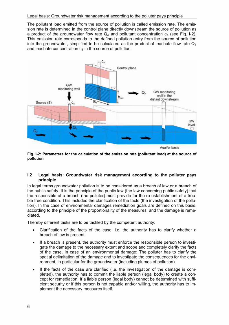
The pollutant load emitted from the source of pollution is called emission rate. The emis-sion rate is determined in the control plane directly downstream the source of pollution as a product of the groundwater flow rate QA and pollutant concentration cA (see Fig. I-2). This emission rate corresponds to the defined pollution entry from the source of pollution into the groundwater, simplified to be calculated as the product of leachate flow rate QS and leachate concentration cS in the source of pollution.
Fig. I-2: Parameters for the calculation of the emission rate (pollutant load) at the source of pollution
I.2 Legal basis: Groundwater risk management according to the polluter pays principle
In legal terms groundwater pollution is to be considered as a breach of law or a breach of the public safety. It is the principle of the public law (the law concerning public safety) that the responsible of a breach (the polluter) must provide for the re-establishment of a trou-ble free condition. This includes the clarification of the facts (the investigation of the pollu-tion). In the case of environmental damages remediation goals are defined on this basis, according to the principle of the proportionality of the measures, and the damage is reme-diated.
Thereby different tasks are to be tackled by the competent authority:
• Clarification of the facts of the case, i.e. the authority has to clarify whether a breach of law is present.
• If a breach is present, the authority must enforce the responsible person to investi-gate the damage to the necessary extent and scope and completely clarify the facts of the case. In case of an environmental damage: The polluter has to clarify the spatial delimitation of the damage and to investigate the consequences for the envi-ronment, in particular for the groundwater (including plumes of pollution).
• If the facts of the case are clarified (i.e. the investigation of the damage is com-pleted), the authority has to commit the liable person (legal body) to create a con-cept for remediation. If a liable person (legal body) cannot be determined with suffi-cient security or if this person is not capable and/or willing, the authority has to im-plement the necessary measures itself.

Legal basis: Groundwater risk management according to the polluter pays principle
7
• The authority has to ensure that the damage is remediated in a sufficient way. The-reby it must keep in mind that in certain cases the polluter’s liability is limited.
• In case of an acute endangerment (e.g. the pollution of waterworks of the public drinking water supply) the authority has to provide immediate corrective actions, as soon as it recognises the acute endangerment, therefore for example to prevent that contaminated water is supplied into the waterworks.
• Finally, the authority is responsible for the supervision of the general groundwater quality.
In Germany, water is treated legally independently of property borders as a public prop-erty, at which there exists no private property. The water authority occupies the function of a guarantor for the groundwater quality (“guarantor position”). As soon as the authority discovers the breach of law, the authority can oblige both the polluter as well as the owner of the property, where the source of pollution is situated, to investigate and remediate the damage. The authority selects the obliged liable person according to its best judgment, i.e. obligates those, who are able earliest to carry out the necessary measures.
In Czech Republic and in Poland the management of groundwater pollution runs similarly as mentioned above. However, there are some exceptions. In Czech Republic in case of historical industrial pollutions originated before 1989 in communistic epoch, the govern-ment in consequence of privatization of state properties guarantees the process of con-tamination investigation, evaluation and remediation according the special Act (Act No. 92/1991 of 26 February 1991). In Poland executive acts are missing.
Risk assessment has an important function to judge whether the groundwater quality is acceptable (no further action) or whether it is so polluted that a breach of law must be assumed. If so, risk assessment leads to the need of further measures and to the selec-tion of remediation goals. In Germany for this purpose threshold values are defined. The evaluation is based on concentration values and (in special cases) on pollutant load val-ues. In the Czech Republic the evaluation is based on assessment of potential risks aris-ing from concentration values and (in special cases) on pollutant load values towards hu-man health and environment protection. In Poland this approach is still waiting for adop-tion.
The current standard “case by case”-management of pollution is derived from the liability of the polluter (polluter pays principle). It concerns thereby a generally used approach in the risk management of environmental damages. In cases of single damages and clear liability the case by case investigation has proved itself well. This strategy starts in the core of the damage, the location of the entry of pollutants into the soil. It pursues the pol-lutant transport beyond the soil passage into the groundwater. It bases on the concept that a pollutant entry always proceeds over a defective plant or in other manner of entry from a certain property. This facilitates the tracing of the entry of pollutants and the effects on the subjects of protection (here in particular on the groundwater) of a traceable trans-port pathway and thus forms a so-called “red thread”. This verification justifies the liability of the polluter besides the liability of the property owner. The standard case by case man-agement is essentially an approach for individual sources of pollution. However, in com-plex cases with multiple sources of pollution this standard approach is often limited and does not allow to identify the key sources of pollutions and the liable polluters.

Limitation of the standard approach for groundwater risk management of sources of pollution
8
I.3 Limitation of the standard approach for groundwater risk management of sources of pollution
The standard approach for risk management of sources of pollution is limited, if
• many different sources of pollution might contribute to an identified groundwater damage, and it is however unclear, which ones are actually liable for the groundwa-ter damage (Fig. I-3),
or if
• many sources of pollution overlay each other and the objective of investigation is to identify the contribution of each source to the entire groundwater damage (Fig. I-3),
or if
• the source of pollution was removed e.g. by excavation, in the larger depth how-ever exist secondary damages (e.g. pools), which can hardly be identified, although they continue to emit pollutants.
Fig. I-3: Neighbouring sources of pollution
In the mentioned cases the authority is challenged by the task to investigate such dam-ages technically, and which one of the potential liable persons must be obliged in which manner (and/or for which measure) for further measures.
Moreover the results of the investigation have to be legally self defensible.

EU water directives: Groundwater bodies and the monitoring of trends
9
Practical implementation problems are (according to the German, Czech and Polish na-tional law):
• The owner liability is restricted to soil damage on the property (damage in the un-saturated zone). The liability for plumes of pollution, which extend beyond the property, is restricted to the polluter.
• The authority is obliged (in Germany among others on the basis of its guarantor position) to investigate and, if necessary due to endangerment of the public safety, to remediate groundwater damages in the public area, if it the polluter cannot be obliged.
• Investors (e.g. building owners) are obliged, in case of groundwater drainage in plumes of pollution (for example temporary draining groundwater for the building pit or permanent draining of buildings), to clean delivered groundwater before the dis-charge. The investor can hold the polluter liable only on the basis of the civil law.
• The authority has problems with the polluter’s identification for plumes of pollution, e.g. groundwater contamination in the public space. Thus the task is to retrace the damage within the framework of official identification of liable persons from the plume back to the source of pollution.
• In complex cases (many neighbouring sources of pollution, see Fig. I-3, and/or complex hydrogeological conditions), the task of clarification of the source – plume relationship is difficult for the competent authority in order to set the appropriate priorities.
• If the primary source of pollution was removed for example within the framework of building activities, frequently secondary sources of pollution remain, which cannot be identified or eliminated by the treatment of the sources of pollution.
In all these mentioned cases an integral groundwater investigation offers a useful and technically suitable option, in order to identify the polluter and to relieve investors or other persons concerned without polluter contribution.
I.4 EU water directives: Groundwater bodies and the monitoring of trends With the water framework directive (2000/60/EC) and the groundwater directive (2006/118/EC) the European Union introduced new aspects and points of view into the investigation and evaluation of the groundwater quality.
The groundwater directive defines threshold values for a “good chemical status” of the groundwater in Article 3 No.1. Quality standards (reference values) are indicated in ap-pendix 1, the list of parameters however is limited to nitrate and pesticides. The ground-water directive obliges the Member States to indicate reference values for the further sub-stances listed in appendix 2 up to 22.12.2008 Among others Sulfate and Chloride are mentioned which are in many cases related to mining activities, as well as tetrachloro-ethylene and trichloroethylene, which produce Europe-wide strongly spread and particu-larly dangerous groundwater pollutions. Although not explicitly mentioned polycyclic aro-matic hydrocarbons are another group of important substances related to e.g. gasworks sites which should be considered in the national listing of threshold values.
Into Article 5 of the groundwater directive the term “plumes of pollution” is introduced. The reduction of the pollutant entry into the groundwater is explained to be a long-term goal
The water framework directive obliges the Member States in Article 17 to establish a good chemical status in the groundwater bodies up to the year 2015 (water framework directive Article 4, No. 1b).
Important strategic elements of the EU-directives are the principle of the view on larger areas and water bodies (in addition to the national view on individual cases, predominat-

The objectives of the groundwater risk management approach
10
ing up to now). This leads to the fact that the Member States must define and examine groundwater bodies (groundwater directive Article 3 No. 1). Thus a scale discussion is to be held. There is the danger of the marginalization of extensive groundwater damages by appropriate scale choice: If the scale will be selected large enough, then pollution will re-main unnoticed.
The groundwater directive introduces the procedure of the trend observation in Article 5. If an increasing concentration of pollutants is discovered by the trend observation, a trend reversal must be achieved.
I.5 The objectives of the groundwater risk management approach A general aim of groundwater management is to obtain good chemical status of the body of groundwater concerned. This requires a survey of the qualitative status and, if neces-sary, a trend description of the groundwater quality. If in polluted groundwater bodies no trend for a qualitatively good condition can be assumed, a trend reversal must be achieved with the long-term objective of a good quality.
The trend reversal will be gained, if the following goals are pursued:
• Prevention of further pollutant impacts.
• Prevention of further pollutant spreading, i.e. further transport of pollutants in the groundwater.
• Remediation of the main sources of pollution.
The integral groundwater investigation facilitates the description of the qualitative condi-tion of a body of groundwater in an efficient way - also beyond a longer time period – and creates thereby an important basis for the trend reversal.
Fig. I-4: The objectives, the tasks and measures of the groundwater risk management

Description of the MAGIC groundwater risk management approach
11
I.6 Description of the MAGIC groundwater risk management approach The integral groundwater investigation is the core element of the MAGIC risk manage-ment approach. This integral investigation requires a reversion of the investigation ap-proach from the individual case related consideration of sources of pollution (case-by-case-approach, source approach) to the integral investigation of the plumes of pollution (integral groundwater investigation).
The description of the approach is made under two aspects:
C strategic tasks
D operational technical measures
In the first part all strategic tasks are listed and described, which are suitable. Which of these tasks in a concrete individual case are to be settled, must be determined in the indi-vidual design depending on the specific characteristics of the investigation area.
For the integral groundwater investigation generally the following strategic tasks can be tackled (see also Fig. I-4):
C1 Record of groundwater quantity and quality: Integral, three-dimensional and simul-taneous recording and description of the groundwater status in the investigation area in terms of quantitative and qualitative aspects. (D1, D2, D3)
C2 Identification of the sources of pollution. (D1, D2, D5)
C3 Interaction between plumes and sources: Identification of Plumes of pollution, de-scription of the interactions in terms of quality and quantity, for example in terms of emis-sion rates (mass fluxes) and plume lengths for the description of the pollution impacts. (D4, D6, D7, D8)
C4 Prioritisation: Ranking of the pollutant impacts to prioritise the particularly relevant sources of pollution on which remedial actions should be concentrated and for the exclu-sion of irrelevant subordinate sources of pollution from the further treatment. (D7, D8, D9)
C5. Remediation of the sources and the plumes of pollution (D9, D10) or implementa-tion of any other kind of measures to be undertaken by the competent authority...
To tackle the strategic tasks, operational technical measures are to be carried out (see Fig. I-4). The measures are described in detail in the technical part of this handbook. De-pending on the single site or area, specific measures have to be selected and compiled depending on the specific local characteristics. Operational technical measures are:
D1 Data collection and –evaluation, monitoring of the groundwater quality, trend observation and evaluation by a survey and summary of all former investigation ac-tivities on contaminated sites, the single sources of pollution and groundwater monitoring wells (results of former investigations).
D2 Compilation and mapping of all available information in a data base and in a GIS: Sources of pollution and groundwater monitoring wells.
D3 Conceptual hydro-geological modelling - Modelling of the hydrogeological settings, the groundwater flow conditions and the quantitative and qualitative status of the ground-water in the different aquifers.
D4 Integral pumping tests - Integral investigation, i.e. the summarising, three-dimensional and simultaneous recording and description of the hydrogeological conditions in the investigation area in terms of quantitative and qualitative aspects.
D5 Delineation of the plumes of pollution with the help of reference values (threshold values, test thresholds), i.e. with the help of concentration values. These are to be speci-fied (up to Nitrate and Pesticides) on the basis of national reference values.

Description of the MAGIC groundwater risk management approach
12
D6 Numerical modelling the plumes of pollution, i.e. development of a conceptual model of the groundwater flow and pollutant transport to the summarizing record, balance and evaluate the transport processes in the groundwater layers (aquifers) and the interac-tions, i.e. the current and/or transport mechanisms including the mass fluxes between the aquifers
D7 Backtracking of the pollutants from the plumes of pollution to the sources of pollu-tion, i.e. clarification of the source – plume relationships. This can be done e.g. via ad-vanced modelling techniques or fingerprinting.
D8 Risk assessment for sources and plumes of pollution using national evaluation tools, if necessary numerical groundwater modelling. Ranking of the pollutant impacts to prioritise the particularly relevant sources of pollution on which remedial actions should be concentrated and for the exclusion of irrelevant subordinate sources of pollution from the further treatment. This procedure implies that relevant sources of pollution emit large and spacious plumes. All other sources of pollution are not relevant for groundwater risk man-agement, nevertheless they can be ecologically important (e.g. on the effect the path soil – human being, which is not regarded here further).
D9 Identification and description of natural retention and degradation processes Natu-ral Attenuation NA.
D10 Development of remediation concepts with concentration on the priorities of the damages, i.e. derivate and evaluate additional needs for action.
Fig. I-5: The key measures and their interactions in the MAGIC groundwater risk manage-ment approach

Characteristics of the integral groundwater investigation
13
The central element of the integral groundwater investigation is the integral pumping test. This test is a powerful measure to investigate source – plume interactions in the ground-water, which is the basis for the assessment of the actual impact of a source of pollution on the groundwater. Prerequisite for the design of the implementation of integral pumping tests is a proper understanding of the hydrogeological setting, which is described in a conceptual hydrogeological model. The results of the pumping tests will vice versa im-prove the model.
The interpretation of the integral pumping tests contributes to the localisation of plumes and their contaminant loads. With the help of backtracking techniques (e.g. fingerprints, modelling approaches) the source – plume interactions can be qualified.
Hydrogeological setting, contaminant loads and source – plume relationship are key input data for the subsequent evaluation, risk assessment and ranking of the sources, which lead to prioritisation of further corrective actions and concrete remediation.
Two different integral investigation approaches are possible:
• For areas, investigated for the first time, the record of the entire plumes of pollution (i.e. the complete recording of the downstream mass flux in the control planes, 100% - recording) is needed.
• For areas with numerous investigation results and detailed knowledge of sources of pollution, a partial, supplementary plume recording in the control planes is suffi-cient. In this context, the results of all of the available investigation data form the data base.
I.7 Characteristics of the integral groundwater investigation The integral groundwater investigation shows the following differences to the conventional “case by case” investigation of pollution sources, which means first searching for sources of pollution and investigation of corresponding plumes in the second step:
• The plumes of pollution will be identified first and based on their characteristics the sources of pollution are determined and evaluated.
• The contaminant mass flow rates of the pollution plumes represent the source im-pact in an appropriate way.
• The source-related consideration taking into account the liability of property owner is tackled after the conclusion of the integral groundwater investigation.
• The integral groundwater investigation requires a stronger commitment of the competent environmental protection authority.
• The treatment of sources of pollution receives a substantially more qualified basis and can be concentrated on the priorities of the pollution. It becomes more efficient and more effective and thereby cheaper.
• The integral investigation facilitates to calculate a balance of the pollutant mass flow rates (balance of emission rates and pollution extraction).
• The integral groundwater investigation facilitates an appropriate and qualified observation and monitoring of the temporal development (significant and sustained upward trend in concentrations of pollutants, trend of the groundwater quality) in a body of groundwater (trend monitoring). Also timely variant and dynamic processes can be tackled in an appropriate way.
Domain of application of the integral groundwater investigation
14
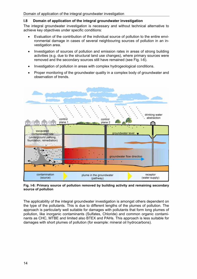
I.8 Domain of application of the integral groundwater investigation The integral groundwater investigation is necessary and without technical alternative to achieve key objectives under specific conditions:
• Evaluation of the contribution of the individual source of pollution to the entire envi-ronmental damage in cases of several neighbouring sources of pollution in an in-vestigation area.
• Investigation of sources of pollution and emission rates in areas of strong building activities (e.g. due to the structural land use changes), where primary sources were removed and the secondary sources still have remained (see Fig. I-6).
• Investigation of pollution in areas with complex hydrogeological conditions.
• Proper monitoring of the groundwater quality in a complex body of groundwater and observation of trends.
Fig. I-6: Primary source of pollution removed by building activity and remaining secondary source of pollution
The applicability of the integral groundwater investigation is amongst others dependent on the type of the pollutants. This is due to different lengths of the plumes of pollution. The approach is particularly well suitable for damages with pollutants that form long plumes of pollution, like inorganic contaminants (Sulfates, Chloride) and common organic contami-nants as CHC, MTBE and limited also BTEX and PAHs. This approach is less suitable for damages with short plumes of pollution (for example: mineral oil hydrocarbons).

Administrative aspects of the implementation of the integral groundwater investigation approach
15
I.9 Administrative aspects of the implementation of the integral groundwater in-vestigation approach
The integral groundwater investigation approach is suitable for
• identification and ranking of sources of pollution as part of the preliminary investiga-tion
• preparation of a complex concept of remediation measures for large areas
as well as for
• observation of the trends of water quality in groundwater bodies according to the water framework directive and the groundwater directive.
Both measures in Germany are in the competence of the environmental protection author-ity.
The integral approach provides the possibility to obtain legally self defensible results.

Principles of integral pumping tests
16
II PART
PART II THE TECHNOLOGY
PLANNING, IMPLEMENTATION AND EVALUATION OF INTEGRAL GROUNDWATER INVESTIGATIONS - IN PARTICULAR BY MEANS OF INTEGRAL PUMPING TESTS.
II.1 Principles of integral pumping tests An explicit aim of MAGIC is to develop comprehensive and reliable tools for site charac-terisation and risk assessment for groundwater contaminations.
A well-established method for performing integral groundwater investigations are so-called integral pumping tests IPT, which are defined as long-term pumping tests with systematic analysis of concentration of contaminants in the pumped water. This methodology proved to be appropriate in recent case studies (e.g. Neckartalprojekt, 1996-99; INCORE, 2000-03, Stuttgart 21, 2002-04). Currently in Baden-Württemberg IPT are used to perform groundwater investigations downgradient of complete urban districts (e.g. northern parts of Ravensburg and Bahnstadt, Albstadt-Ebingen). Due to these positive experiences this investigation method should be made available for a wide spectrum of applicants.
Part II of this handbook describes the basic conditions for integral pumping tests and the related steps of design. The main focus is on planning, performance and interpretation of integral pumping tests. The range of application for two dimensional analytical and nu-merical interpretation will be outlined and the MAGIC-software tool described and demon-strated.
Expanding integral groundwater investigations into three dimensions and thus allowing depth-dependent differentiation is a matter of current research. It is not included in this report. Nor are temporal integral investigations (e.g. dosimeter measurements) included.
Chapter II.1 provides background information, introduces the principles of integral pump-ing test and defines key technical terms hence providing basic information. Chapter II.2, applications and limitations, defines the range of applications and the limitations of the technology related to the different scales of investigation areas to be considered.
The handbook then focuses on all aspects of practical implementation, introducing the procedure in a stepwise approach. In the first step (chapter II.3) objectives and the areas to be considered have to be defined and existing data are to be collected. Setting up a conceptual hydrogeological model comprises the second step (chapter II.4). The concep-tual hydrogeological model is prerequisite for all following steps and a crucial element in the whole procedure. Chapter II.5 introduces all planning activities required to ensure a proper investigation campaign, which is the third step. The fourth step (chapter II.6) deals with field work related aspects, describing all practical aspects as equipment, sampling procedures, monitoring and control etc. incl. QA/QC aspects.
The fifth step, Interpretation of the IPTs, is laid down in detail in chapter II.7, which con-tains relevant hydraulic interpretation approaches based on analytical tools, the interpreta-tion of combined tracer test and the possibilities of numerical interpretation of IPTs. More-over the application of the MAGIC-software tool is described. The software is designed to provide an easy to handle tool to be applied in daily practice for planning, performance and interpretation of integral pumping tests.
Since 1997 the chair of applied geology at Universität Tübingen has been developing a methodology for spatially integral groundwater investigation (PTAK & TEUTSCH, 1997, SCHWARZ, PTAK & TEUTSCH, 1997a, b, HOLDER et al. 1998, HOLDER & TEUTSCH 1999, TEUTSCH et. al., 2000, PTAK et al., 2000, PTAK & TEUTSCH, 2000, JARSJÖ et al. 2002, BAYER-RAICH et al., 2003, 2004). This methodology is known as integral pumping test IPT. These developments were accompanied by the practical implementation, which was from

Principles of integral pumping tests
17
the beginning strongly supported by the Amt für Umweltschutz, Landeshauptstadt Stutt-gart within the frame of the projects Neckartalaue 1996-1999 and INCORE 2000-2003.
The method of integral pumping test employs the effect of the increasing capture zone during a pumping test. Simultaneously with the pumping time multiple contaminant con-centration measurements are performed. This allows estimating the spatial distribution of the contaminants and the total mass flow rate of a contaminant plume in groundwater.
The aquifer in the vicinity of pumped well is affected with the long term pumping of groundwater. The capture zone is increasing according to hydrogeological condition of the aquifer and to the parameters of pumping specification with the pumping time.
Fig. II-1: Comprise of downgradient area with capture zone of a single well
In simple cases the capture zone of a single well comprises the whole area downgradient a suspicious site after a certain pumping time (see Fig. II-1). The quality of groundwater in

Principles of integral pumping tests
18
the specific time interval corresponds with the spatial integral quality in the capture zone which diameter is determined according to the Bear & Jacobs formula:
W = Q/(kf x I x m)
Q: pumping rate [L3/T]
Kf: hydraulic permeability of aquifer [L/T]
I: Gradient [L/L]
m: aquifer thickness [L]
W: width of capture zone
In geometrical terms, W is the diameter of the capture zone in cylindrical cases.
Fig. II-2: Principle of steady-state integral measurement (TEUTSCH et al. 2000, updated )
As practical experience shows, covering the whole area downgradient of a potentially con-taminated site with one pumping test is usually not possible. On the one hand plume loca-tions usually cannot be estimated exactly enough as to optimally locate a extraction well. On the other hand very long pumping times would be necessary to achieve a quasi-steady state situation.
Using the sampling and analysis of groundwater in the specified time intervals during the pumping (the multiple concentration measurement) the information of the quality of groundwater related to the specific capture zone can be received. The time curve of con-taminant concentration indicates the occurrence of an important variation in groundwater quality (the occurrence of the contaminant plume) in the capture zone of pumping.

Principles of integral pumping tests
19
Fig. II-3: Relation between measured and real concentrations (acc. to BOCKELMANN et al., 2001)
The concentration time series yield information on the position and extent of the contami-nant plume(s) as well as on the concentration of the target substances in the plume(s).The typical examples of the time concentration curves resulting from the position of the extraction well and the spatial occurrence of contaminant plume are illustrated in Fig. II-4.
1
Con
cent
ratio
n
Time
Groundwater flow directionPlume of pollution
Extraction well
Maximal Isochrones
3
Con
cent
ratio
n
Time
4
Con
cent
ratio
n
Time
2
Con
cent
ratio
n
Time
Fig. II-4: Characteristic hydrograph curve for concentrations with different capture zone geometries (acc. to HOLDER & TEUTSCH, 1999)
With an inverse method the possible distribution of contaminants in the capture zone of a well can be calculated. This allows to calculate the average contaminant concentration CAV in the capture zone and mass flow rates QA*CAV

Applications and Limitations
20
II.2 Applications and Limitations
II.2.1 Scale of investigation According to the MAGIC approach, integral groundwater investigations are basically ap-plicable in two different scales. In a large-dimensional-scale (industrial areas, town dis-tricts, etc.) they are capable to delineate zones of no or little groundwater contamination from zones of significant contamination (screening). By an overall definition of mass flow rates and contaminant concentrations a first risk assessment; ranking and determination of priorities for further activities is possible.
If applied at small scale or for single site characterisation, main focus of the integral inves-tigation is to assess contaminant mass flow rates besides concentrations for a better risk assessment, to identify plumes of groundwater contamination origination at the site, hence ensuring to measure the total impact of groundwater pollution from the site.
Fig. II-5: Example of an integral groundwater investigation at small scale in Ostrava

Applications and Limitations
21
Fig. II-6: Example of an integral groundwater investigation at large-dimension-scale in Stutt-gart-Feuerbach (base map by Stadtmessungsamt Stuttgart)
Nevertheless especially when applying the tool in a large-dimensional-scale, contaminant-specific plume lengths are to be taken into account. Organic contaminants at least show a decrease of concentrations downgradient from the contaminant source under natural con-ditions. Having acquired a certain downgradient distance to the source, a contaminant cannot be detected any more (plume length). Different surveys show contaminant plume lengths for different compounds (see Fig. II-7, TEUTSCH et al. 1997 and STUPP & PAUS 1999).

Applications and Limitations
22
0 500 1000 1500 2000 2500
Plume length in m
CHC
Phenols
Benzene
BTEX
PAH
Con
tam
inan
ts
High water solubility, low retardation, slow degradation
High water solubility, low retardation, fast degradation
Water solubility, retardation and degradation differ over several orders of magnitudes -high uncertainties of field data
? ?
Contaminant Properties
N=80 (107)
N=12 (18)
N=21 (27)
N=79 (96)
5-Ring 2-Ring 3-Ring
Fig. II-7: Statistical plume lengths (acc. to TEUTSCH et al. 1997)
Table II-1 summarises results of both surveys. Table II-1: Statistical plume lengths (acc. to TEUTSCH et al. 1997, STUPP & PAUS 1999)
Contaminant
TEUTSCH et al.(1997)
75 % of cases
Stupp & Paus (1999)
average
Stupp & Paus (1999)
range
CHC 2150 m 1100 m 50 to 8000 m
BTEX 420 m 141 m 10 to 400 m
TPH - 55 m 10 to 160 m
PAH 300 m 127 m 50 to 300 m
Plume lengths calculated in the surveys depend on contaminant properties, source strengths, redox conditions in the aquifers, flow velocities, analytical limits of determina-tion and further aspects of the single cases considered. Notwithstanding the scattering of values in table II-1 the relationship between different substance groups is clear and re-flects the general behaviour of degradation and retention.
When defining control planes different plume lengths are to be taken in account. For ex-ample it makes no sense installing a control plain for petroleum-derived hydrocarbons in 200 m distance from the source, because there are no measurable hydrocarbon concen-trations to be expected any more.
Referring to statistical plume lengths special evaluation methods can determine those areas with a high probability of groundwater pollution (backtracking). In a reverse conclu-sion, areas with a high probability of no or irrelevant groundwater pollution can be identi-fied. Thus integral groundwater investigations can be used in a large-dimension-scale to confirm or disprove potential contamination regarding the pathway soil-groundwater.
In the latter case an investigation of potentially contaminated areas is not necessary even for the pathway mentioned. This means a relevant cost reduction. In case of a pollution to

Applications and Limitations
23
be confirmed, further investigations in a small dimensional scale are necessary. Integral groundwater investigations proximately downgradient of potentially contaminated areas help to define the source strengths of contaminant sources. By determining mass flow rates and average concentrations a risk assessment is possible.
Natural attenuation processes can be investigated by an investigation based on two or more control planes. A decrease of mass flow rates along groundwater flow direction indi-cates natural retention (natural attenuation). However this requires an exact definition of mass flow rates across the control planes. Mass balances can be additionally verified by investigations of redox conditions (e.g. O2, NO3, NO2, NH4, SO2, H2S) as well as isotope measurements of water (e.g. δ18O, 3H) and contaminant molecules (e.g. δ13C), which are both sensitive parameters indicating biodegradation processes.
II.2.2 Range of application Integral pumping tests are generally applicable within a broad range of hydrogeological and technical conditions. Key criteria are the extension of the potential plumes related to the width of captures zones which can be achieved by the pumping tests. Table II-2: Range of applications based on hydraulic and chemical criteria
Range of IPT application from to
Hydrogeological conditions
⌧ hydraulic coefficient - kf (m/s) 10-6 10-2
⌧ hydraulic gradient - I < 0.01
⌧ effective porosity - ne < 0.2
Pollutants
⌧ soluble in water
⌧ low sorption, low degradability
major ions, inorganic salts, naphthalene, ben-zene, chlorinated hydro-carbons etc.
⌧ octanol-water partition coefficient Kow logKow < 3
Integral pumping tests are not useful in situations when only very small widths of capture zones can be achieved. Low permeabilities (kf < ca. 1E-6 m/s) give unfavourable condi-tions for this method. Another disadvantage is a very high yield (Kf > ca.1E-2 m/s). Due to high pumping rates there are considerable amounts of water to be cleaned and/or dis-charged, causing high costs. Furthermore narrow plumes of contaminants with low trigger values (e.g. PAH or pesticides) might not be detectable due to dilution effects combined with analytical detection limits.
A further condition for performing an integral pumping test is if the water head in the pumping is well high enough to enable pumping with a sufficient drawdown. The expected depression of the groundwater level in the extraction well can be calculated. The well has to be yielding enough as well as the static water column in well has to be thick enough to enable pumping with a sufficient drawdown. For example a water column of 1.5 m high would not meet this condition.
It is also problematic if aquifer thickness is too high, because pumping tests are depth-integrating. Contaminant plumes with small vertical extent might not be discovered, be-cause their concentrations might fall below detection limits due to dilution. Moreover hy-

First Step – Basic Assumptions and Investigations
24
draulic connections between different aquifer layers or from aquifers to surface waters might influence measurement results and lead to misinterpretations.
In the immediate vicinity of LNAPLs planning and performance of pumping test has to be handled with great care. A displacement of free phase LNAPLs within the capture zone, possibly causing contamination of deeper aquifer levels, has to be prevented. Therefore in case of LNAPLs this method should be applied only in exceptional cases.
Retardation of contaminants (depending on specific compounds and aquifer matrix) usu-ally can be neglected. Nevertheless a very strong retardation can lead to a misinterpreta-tion due to chromatography effects.
In cases of small-scale-investigations and smooth hydraulic gradients even small meas-urement mistakes strongly influence the calculated groundwater flow direction. Surveying and mapping the location of monitoring wells and measuring hydraulic heads therefore is to be done with very high precision. Otherwise the real groundwater flow direction might not be recognised.
II.3 First Step – Basic Assumptions and Investigations
II.3.1 Definition of objectives and investigation areas To start any activity the project area and their boundaries should be clearly defined. Within this area existing and future use of land and groundwater shall be defined. So the objec-tives for groundwater risk management as well as for the integral groundwater investiga-tion activities in the area under consideration can be derived.
For small scale application of the integral groundwater investigation at single sites the use of a numerical model will not be obligatory to calculate mass flow rates, concentration distribution patterns and the localisation of plumes. This can be approximately done by the means of analytical interpretation. For the characterisation of large areas inclusive de-lineation of plumes and all backtracking options the use of a numerical model will be inevi-table.
After having defined investigation areas and objectives, a rough calculation of related costs can to be done. According to INCORE 2003, as a rough estimate the total integral groundwater investigation costs (incl. modelling, analysis, fingerprints etc.) can be broken down to about 300 € per m length of control planes or 20,000 € per well to be investigated by an integral pumping test.
II.3.2 Data collection, basic investigation A reliable planning of integral pumping tests requires a profound conceptual hydro-geological model (see chapter II.4). Thus all existing data about geometry of aquifers to be considered, groundwater flow and transport conditions, position of potentially contami-nated areas and compound-specific properties (statistical plume lengths, see table II-1) have to be collected and evaluated. Knowledge gaps have to be filled. Therefore basic investigations and setting up a conceptual hydrogeological model is in most cases an it-erative process.
Key hydrogeological properties which are needed for the subsequent steps are
• hydraulic conductivity,
• aquifer thickness,
• hydraulic gradient under uninfluenced conditions,
• effective porosity,
• appropriate pumping time and rate.

Second Step – Conceptual Hydrogeological Model
25
The magnitude of pumping rate is defined by factors like hydraulic conductivity, well de-sign and feasible drawdown. An exact estimation of the width of capture zones to be achieved by an integral pumping test and the shape of the depression cone is depending on the accuracy of available data. Therefore a thorough evaluation of existing data is re-quired
The exploitation of site maps, strata profiles and well design plots are prerequisite for the conceptual model’s establishment. The actual state of monitoring wells has to be checked, hydraulic heads and depth of wells to be measured. The availability of a reference date measurements of hydraulic heads in the investigation area is a basic need. A contour map of the water table (hydraulic heads or isohypses) is created, based on the evaluation of reference date measurements. After plausibility check of measured data some monitoring wells might need a check of their measured hydraulic head.
For economical reasons already existing monitoring well should be used if possible. Moni-toring wells to be used as extraction wells should have a diameter of at least DN 125 or better DN 150. Therefore in this phase of planning a detailed survey of existing infrastruc-ture is required. Monitoring wells have to be checked for their ability to function as an ex-traction or observation well.
If sufficiently reliable specific aquifer parameters are not abundant, field tests have to be performed. Permeability can be gained from short-time-pumping tests, tracer tests are to be done to acquire values of effective porosity. For a first assessment of contamination groundwater samples are to be taken. Sampling time should be synchronous with pump-ing start and end respectively. Water samples should be analysed for the relevant pa-rameters.
In case of an anticipated contamination in deeper aquifer layers, a decision about their potential investigation is necessary. Due to different hydraulic conditions (hydraulic con-ductivity, direction of flow and hydraulic gradient) a separate inspection of each layer is needed. This requires separate monitoring wells for each layer.
Besides technical and hydraulic aspects retardation of contaminants might be a relevant factor. Especially a high content of organic material in the aquifer matrix (peat, sapropel, coal, etc.) will affect the transport of contaminants with high retardation (e.g. some PAHs), if wells are too far apart from each other. Due to chromatographic effects the concentra-tion-time series of the extraction well will not represent the spatial distribution of contami-nants in the aquifer.
II.4 Second Step – Conceptual Hydrogeological Model Planning an integral groundwater investigation requires a proper understanding of the system. In recent years the tool “conceptual site model” or “hydrogeological model” has been established. For the hydrogeologist it can be an independent tool but also a prelimi-nary step for a numerical model.
A conceptual hydrogeological model presents spatial illustration of all relevant site specific conditions. The data are presented in an abstract and schematic way (FH-DGG 1999, 2000a, b). For illustration, Fig. II-8 shows an example how data are handled to create zones of mostly homogeneous properties.

Second Step – Conceptual Hydrogeological Model
26
Aquitat
Hydrostratigraphic unit
Aquifer
10 [m/s] 5 10 [m/s] Homogenous zone
-6 - 4
1 10 [m/s] -5 2 10 [m/s] - 5
Aquifer
Aquitat
Aquifer
Aquitat
Aquitat Aquifer
Aquifer
Mudstone
Sandstone Mudstone Quaternary (q)
0 250 500 1000 1250 1500 1750 [m] 200 210 220 230 240 250 260 270 280 290 300
[mNN] M2
Measuring M1 M3 Well
River Points
Model border
kbu kc kbl
Triassic sandstone }
Geological underground conditions Hydrostratigraphic Hydrogeological model Units
Fig. II-8: Abstraction procedures for definition of homogeneous zones and related quantified parameters
Thus it presents the essential properties of a system, giving reliable information to de-scribe and predict hydrogeological processes with their spatial and temporal dimensions. It gives consistent information about aquifer geometry (hydrostratigraphy, geological bar-riers, see Fig. II-8), geohydraulics (groundwater flow, type of aquifer, hydrogeological pa-rameters including spatial distribution) and about water balance.
First step of investigation is the screening and evaluation of existing information at local and regional scale, as e.g. topographical and geological maps, contour maps of the water table and other hydrogeological maps, city maps, data about groundwater recharge, water protection areas, construction plots of relevant buildings and plants, plots of lines and un-derground conduits, strata profiles and protocols, monitoring well design protocols, sam-pling and pumping test protocols, analytical results, compound specific information data, investigation reports, hydrogeological surveys and expertises, comments of administrative bodies, etc.
If this information is not complete or not sufficient to develop an appropriate and compre-hensive conceptual model, even in the first phase of planning additional field measure-ments, as for example reference date measurements, have to be performed. Possibly in a further step a basic numerical model is built on the hydrogeological model.
Documentation of the hydrogeological model has to mention the origin of used data and give a transparent and comprehensive argumentation leading to final conclusions.
Geometry of aquifer / spatially limited sedimentation / tectonic displacement (secondary) / thickness differences due to conditions of sedimentation / sedimentation conditions vary-ing in lateral extent

Second Step – Conceptual Hydrogeological Model
27
Fig. II-9: Geometry of aquifer presented in a schematised way (UFRECHT, unpublished )
Frequently a lithological cross section is used to visualise geologic and hydrogeological data. Mainly sections from control planes give a good view of hydraulic conditions espe-cially when data from hydrostratigraphic formations are presented in an abstract way (see figures II.7-10).
Fig. II-10: Lithological cross sections of the MAGIC area in Olsztyn
Spatially limited
sedimentation
Tectonic
Displacement
(secondary)
thickness differences
due to conditions
of sedimentation
sedimentation condi-tions varying in lateralextent
Third Step – Planning of integral pumping tests
28
The conceptual model enables to visualise all relevant site conditions in a spatial dimen-sion. It serves as a basic planning and evaluation tool for all further planning steps. Estab-lishing a conceptual model is an iterative process. The first draft is usually based on a lot of assumptions, being replaced by facts with increasing information level. Thus the con-ceptual model gets continuously updated during the whole planning and investigation process.
When investigating contaminated sites, the hydrogeological model enables comprehen-sive information about contamination sources and polluters, about relevant compounds and their fate and behaviour. In order to answer questions about compound-specific be-haviour in the aquifer (transport and degradation of contaminants), reliable hydrochemical data (redox conditions, concentration distribution of geogenic and anthropogenic com-pounds) have to be included in the hydrogeological model.
II.5 Third Step – Planning of integral pumping tests
II.5.1 Definition of control planes Control planes are vertical cross-sections through the groundwater aquifer. The most im-portant results related to control planes are contaminant mass flow rates across the con-trol plane as well as average and maximum concentrations. These values are supposed to characterise the emission and source strength of the contaminant from the investigated source zone(s). Therefore, it is important to ensure that control planes:
• are placed downstream the investigated source zone(s)
• cover total width of groundwater stream that might be contaminated by the source zone(s)
• are as much as possible perpendicular to groundwater flow direction
For ensuring mentioned features of control planes, their definition should be based on detail analysis of the conceptual hydrogeological model.
Referring to chapter II.2.1 the scale of application and the distance between downgradient control planes is a key issue. Aiming at a precise quantification of the source strength not influenced by natural attenuation processes along the flow path a first control plane should be located closely downstream of the potential sources of pollution. Further downgradient control planes to delineate the plumes and to quantify natural attenuation processes should be defined according to the contaminants considered. In case of CHC a distance between control planes of up to 500 -1000 m can be appropriate, whereas for BTEX and PAHs 100 – 150 m should be considered as a maximum. If complex plume patterns and interactions of plumes are to be expected, the control planes should be located in closer distances.

Third Step – Planning of integral pumping tests
29
Fig. II-11: Defining the control planes in Feuerbach
Planning also implies the expected magnitude of contaminant concentrations and pump-ing rates. Especially in locations near to the plume edge concentrations might fall below the detection limits with increasing pumping rates. In these cases, no complete interpreta-tion of the pumping test is possible. Also should be checked if there is a sufficient number of available monitoring wells (three to five) in the vicinity of the control planes. The obser-vation of wells is necessary for sufficiently recording the hydraulic system’s response to pumping and for a sufficient data evaluation (see chapter II.7.1). Furthermore drawdown in different observation wells provides an indication for the depression’s geometry.
II.5.2 Hydraulic planning The aim of planning process is to define the crucial parameters of future IPTs, such as:
• number of wells to be used
• pumping rates
• duration of pumping test
• number of samples
• timing of particular samples
During planning process one should also keep in mind the technical constrains of integral pumping tests application. Also a compromise between scientific & legal requirements and the need for minimising the costs have to be achieved.
Technical constrains are usually linked to drilling the wells, operating the pumps, maintain-ing the pumped water and sampling. It should be taken into consideration that in some

Third Step – Planning of integral pumping tests
30
places drilling is very difficult (e.g. in industrial area there are a lot of areas full of concrete and underground installations). In case previously existing wells are planned to be used the well diameter might not allow the installation of a powerful pump to achieve desirable pumping rates. In other cases the amount of water to be pumped cannot be beard by the local sewage system. As regards sampling, overnight or weekend sampling might be diffi-cult to organise and therefore should be avoided, if possible.
Scientific requirements are fulfilled if the integral pumping test can provide reliable infor-mation about groundwater contamination downstream the investigated source zone. In EU countries and regions so far there are no detail regulations about percentage of the poten-tially polluted groundwater area to be covered by groundwater investigations. According to the experiences made in Baden-Württemberg with the application of integral pumping tests we would recommend
- to cover more or less 100 % of the investigation area in cases with only few pre-existing data from point measurements .
- to cover even less than 50 % in cases with a high level of pre-existing knowl-edge and if an appropriate numerical model is part of the integral groundwater investigation.
Fig. II-12: Coverage of groundwater stream by the integral pumping tests
The costs of integral pumping tests are an important factor and it is obvious that they should be minimised whenever possible. The main sources of the costs are: drilling the wells, hiring/buying/operating the pumps, personnel for supervising the pumping and sampling, analysing the groundwater samples and finally (if needed) treatment and sew-erage of pumped groundwater. Spending e.g. more money on drilling more wells can re-duce the costs of pumping (shorter pumping, or pumping with lower rate) with the same level of gained information.

Third Step – Planning of integral pumping tests
31
Therefore, optimal planning of integral pumping tests is a time-consuming iterative proc-ess. In order to facilitate it, several approaches have been used so far (CSTREAM, ROTHSCHINK-UW, modelling, see chapter II.7). The MAGIC software tool for integral pumping tests planning and interpretation has been developed by team of Central Mining Institute, Katowice, Poland. Basing on convergent flow equations (BEAR & JACOBS, 1965) further evaluated by University of Tübingen (BAYER-RAICH) and starting from the algorithm by ROTHSCHINK-UW, a user friendly GIS-based software in Java environment have been created. On following pages the planning and interpretation of integral pumping tests us-ing this software is described.
Input Parameters
Basic parameters have to be inserted first (Fig. II-13). They can be divided into 2 groups:
• independent hydraulic parameters: effective porosity [n] , hydraulic conductivity. [K], hydraulic gradient [i] and aquifer thickness,
• pumping parameters: pumping rate [Q], total time of IPT, number of samples.
Accordance of input parameter units should be checked. The next needed data is the set of times at which each of planned samples is going to be taken.
Fig. II-13: Planning of integral pumping tests using MAGIC software tool.
Figures at the bottom of the dialog window help to imagine how the changes of input pa-rameters affect the values interesting for planning purposes, such as: width of capture zone at given time step and increase of this width between subsequent time steps. The times of sampling should be planned in such way, that increase of width does not change significantly during whole IPT.
With steep hydraulic gradients, low permeability-values and small pumping rates the pumping test reaches the quasi-steady state very quickly. The capture zone width then

Third Step – Planning of integral pumping tests
32
does not increase any more. Longer pumping times would only cause costs but spend no additional information.
Should detailed planning show, that investigation targets cannot be achieved with the provisional investigation program, modifications to pumping parameters should be done. Possibly the investigation target can be achieved with a longer pumping time, otherwise additional extraction wells are necessary.
II.5.3 Detailed design of sampling, analytic schedule, quality management A successful interpretation of IPTs is strongly influenced by the quality of groundwater samples taken. The procedures and methods applied for obtaining the input data could affect the reliability of the interpretation of integral pumping tests. It is necessary to apply the principles of quality assessment of sampling and analytical works (Program QA/QC) with the implementation of integral pumping test Method. The goal of QA/QC program is to quantify the uncertainty of received populations of data. Conclusions issued from data without evaluation of uncertainty of results (from sampling and analytical works) will miss the requested reliability.
All activities connected with the sampling, handling of samples, with the preparation of sampling equipments etc., should be implemented according to standardised procedures or standards to eliminate the total uncertainty of the field works. It should be assured with the selection of applied procedures that these procedures comply with the purpose of in-vestigation and they are suitable for that. The special attention should be paid to the pro-cedures of sampling of unstable parameters (e.g. volatile organic compounds etc.).
A detailed sampling and analysing plan has to be done in coordination with the analytical laboratory. Besides the relevant contaminants special laboratory tests might be recom-mendable, i.e. for hydrochemical parameters, redox-sensitive anorganic compounds me-tabolites, trace substances or isotopes. These additional results allow a better understanding of the system in special cases, e.g. regarding exchange of groundwater with other aquifers or surface waters, degradation and retention processes.
For the analysis plan detection limits for specific parameters should be considered. Ex-perience shows a clear trend in the time-concentration-graph only with concentration lev-els in a magnitude two to three times higher than the detection limit. On the other hand analytical detection limits should be about ten times lower than the specific trigger values in order to allow even small plumes to be recognised. This might be problematic for con-taminants with low trigger values (e.g. PAH’s and pesticides). Design of sampling and analysing plan has to be done in a comprehensible manner. An early coordination with the analytical laboratory is required to determine sampling time and sample transport.
The detailed sampling and analysing plan should clearly indicate procedures for samples identification, preservation of samples, appropriate storing and transport as well as quality assurance and control. The general recommendations arising from Standard ISO 5667-14 for QA/QC of sampling and analysis should be applied:
Sampling QA/QC
1) Transport blanks – for each sampling series/day
2) Duplicate samples
a. Standard samples: 1 duplicate on 20 taken samples,
b. Non-standard: 1 duplicate on 10 taken samples,
c. Daily frequency (recommended): 1 duplicate for each sampling day
3) Contaminated samples strictly transport separately from “clean” samples (e.g. in separate transporting boxes).
4) Use EN/ISO standard methods for sampling, if available.

Third Step – Planning of integral pumping tests
33
5) Use only appropriate and decontaminated sampling equipments.
Analytical QA/QC
Principally, it is given in accordance with implemented laboratory quality system (EN ISO/IEC 17025).
It is recommended to be about 5% control samples for each parameter, consisting of:
1) Blank sample from chemicals and glassware,
2) Use of certified reference material or standard (as available), accuracy
3) Duplicate sample, precision
4) Matrix effects (spikes), recovery
Table II-3: Specific Sampling Criteria for parameters investigated in MAGIC
VOCs PAHs Metals Sampling vessel (glass/plastic) +++
Special bottles with PTFE septum
+ Bottles from dark
glass
+ Plastic
Purity of sampling bottle (glass/plastic) All sampling vessels to be delivered from laboratory, specially treated; concentration levels respected.
++ ++ ++
Delay between sampling and analysis (Tr=Transport, An=Analysis, Pr=Preservation)
+++ Tr: immediate, An: 24-
48 hours, If “Pr”, than 7 days (EN
ISO 5667-3)
++ An: 24 hours
+ Pr: 2M HNO3
Cooling during the transport, temperature (generally) Recommended 1-5ºC.
+++ ++ 0
Depth of sampling (presence of the film on the surface) To be taken ONLY water phase (if possible)
+++ +++ 0
Sorption on surface of sampling equipment and/or sampling vessels Danger of cross-contamination. If necessary, rinse sampling equipment before sampling. Use ONLY appropriate sampling vessels prepared by laboratory
+ +++ +
Prevention of interaction sample with AIR +++ Cap with PTFE septum
+ 0
Prevention of visible/UV light + +++ Dark glass
0
Presence of active carbon (“oil” surface in general) 1 + +++ +
Presence of surfactants and humic acids2 + ++ + Presence of suspended solids3 + ++ +++ Two and more phases in sample4 ++
No filtration +++
No filtration +++
Filtration5, 45 μm cellulose filter
Oxidation (chemical/biochemical + ++ ++ Oxidation of some metal ions leads to coagulation
+++ Strong influence on analytical result quality (more than 30% uncertainty; not rare 50-100%
uncertainty) ++ Elevated influence on analytical result quality (magnitude of 10-30% uncertainty) + Normal influence on analytical result quality (magnitude of units % of uncertainty)
0 No serious influence on analytical result quality
1 Samples treatment strictly as at the case of multi-phase samples
2 Samples treatment as at the case of multi-phase samples – removal foam/surfactant of organic phase from surface. Analysis of water phase only.
3 Samples treatment strictly as at the case of multi-phase samples
4 Separation of phases; water phase to be analysed separately. Please, note about estimated amount of phase.
5 On site recommended Possible health risks and safety measures have to be considered too.

Third Step – Planning of integral pumping tests
34
Water authorities should be informed about the investigations planned according to legal requirements. The legal application for pumping might include analytical results from well performance tests. Thus it can be assessed whether a clean-up is required before discharging the pumped water back into the aquifer or to the sewage system.
II.5.4 Planning of tracer tests Knowledge of effective porosity ne is very important for definition of capture zones for IPTs. Together with dispersivity αL it is a fundamental factor for quantifying contaminant emissions. Therefore in the course of IPTs a representative number of tracer tests should be done to determine transport parameters.
The radial flow field developing around a well during an IPT should be used for a tracer test. The monitoring well selected for tracer injection should be located inside the capture zone. Furthermore tracer injection well and extraction well should have the same screen-ing depths. The minimum distance from injection well to extraction well should be two or three times higher than aquifer thickness. This is necessary for having a representative aquifer section and for minimising the influence of vertical flow components. Distance should be only so far, that nearly all introduced tracer masses reach the extraction well during tracer test time. This assessment is an object of preliminary planning (see below). The injection well has to be positioned within the radial flow field, i.e. in the direct vicinity of a well, if, as suggested, transport parameters are to be calculated from tracer passage data in an analytical evaluation. This is shown by concentric isochrones (see preliminary hydraulic planning).
Substances enabling immediate or even on-line measurement of their passage in the ex-traction well during the IPT should be used as tracers. Sodium chloride can be detected by measuring of electric conductivity, fluorescence tracers can be measured by fluorime-ters, bromide ion tracers (e.g. LiBr, NaBr, KBr salts) can be directly evaluated by ion-selective electrode (ISE) method. For reasons of simple handling and low costs Sodium chloride is an approved tracer testing substance during an IPT.
Usually tracer injection is done on the second day of an IPT. By the observation of the drawdown characteristics in the injection well and maybe further monitoring wells around it can be checked whether an appropriate depression cone has developed. This is a pre-condition for tracer transport. The tracer test has to be planned according to the equation of mass transport in a radial flow field (SAUTY 1980):
( ) ( )mrn
Qumittu
turtutQ
rMtrc
eLL πααπ=⎟
⎟⎠
⎞⎜⎜⎝
⎛ −−=
4exp
2,
2
with:
c concentration of tracer in pumped well [kg/m³]
r distance of pumped well to input well
t time after tracer input [s]
M quantity of tracer [kg]
Q pumping rate [m³/s
αL dispersivity [m]
m aquifer thickness [m]
ne effective porosity

Fourth Step - Performance of integral pumping tests
35
Aquifer thickness, pumping rate and distance are given, effective porosity and dispersivity are estimated. The selected tracer quantity should ensure a detectable tracer passage in the pumped well. Furthermore the pumping time chosen has to guarantee a complete tracer passage. In some cases pumping time needs extending and/or distance between pumped well and tracer input point needs reduction.
Sodium chloride in the pumped well should cause an increase in hydraulic conductivity of at least ten to thirty μS/cm or rather 2-5% of the background value.
Conversion of NaCl-concentration to electrical conductivity follows the equation (BLÜMLING & HUFSCHMIED, 1989):
C [kg/m³] = σ(20°) [µS/cm]/1870
II.5.5 Logistics Implementation design has to take logistic aspects of sampling into account. To achieve a maximum of capture zone width in a preferably short time interval, pumping rate should be kept as high as possible. Pumping tests should not last longer than five days to avoid weekend work (frequently no accessibility of company premises, additional costs). Fur-thermore selected sampling times should avoid night shifts.
Finally instruments for investigation performance are listed and dimensioned (pumps, in-ductive flow measurement device, data logger, hose lines, sampling vials, possibly a wa-ter remediation plant, power set, etc.
Accessibility for the planned investigation date (e.g. factory premises, traffic routes, car parks, etc.) has to be checked. Electricity should be abundant and there should be a facil-ity for discharging pumped water (river, sewer system, etc.). Also should be checked if a location for positioning the pumping test equipment is available. Official approvals or per-missions have to be acquired, if necessary. Security barriers for i.e. car parks, pedestri-ans, traffic, etc. have to be prepared.
II.6 Fourth Step - Performance of integral pumping tests
II.6.1 Implementation of integral pumping tests Based on the experiences gained within recent years of performing IPTs the optimal re-quirements for equipment for IPT monitoring can be described as follows:
During the test pumping rates are measured continuously with an inductive flow meas-urement device inclusive digital logging. Physical-chemical on-site-parameters (tempera-ture, pH-value, electric conductivity, dissolved oxygen and redox potential) should be measured and recorded.
Hydraulic heads in extraction wells and related wells in close vicinity should be measured at least by hand before starting the pumping test. During the tests they are measured with pressure-sensitive devices with integrated logging and digital recording. Accuracy of measurements should be at least 1 mm. Timely resolution should be at least one second for the key phase of drawdown and the recovery phase, and about 60 seconds in be-tween. Recovery has to be measured at least for 24 hours after pumping. Measurements should be performed in the extraction well and related monitoring wells.
A preliminary estimation of achievable drawdown boundaries should already be done on site during the pumping campaign. This enables the geologist to modify pumping rates, sampling times and test duration according to current conditions.
A documentation in appropriate protocols has to be done for all measurements and sam-pling procedures performed. Relevant guidelines for performing pumping test and groundwater sampling should strictly be followed.

Fourth Step - Performance of integral pumping tests
36
The sampling works are implemented in a strait cooperation with the analytical laboratory and in accordance to the sampling and analysis plan, see chapter II.5.3
The basic equipment required for an optimal performance of IPTs is listed in the following table.
Table II-4: Basic equipment for an optimal IPT
Purpose, function Equipment device Key feature to be considered
Groundwater level measurement - monitor-ing
Water level data log-ger for continuing groundwater level measurement and registration
• Accuracy of measurements should be at least 1 mm
• Timely resolution should be at least one second for the key phase of drawdown and the recovery phase, and about 60 seconds in between
• Recovery has to be measured at least for 24 hours after pumping
• Measurements should be performed in the pumping well and related monitoring wells
Submersible pump • With appropriate flow rate range (up to 20 m3/h)
• Centrifugal pump system • Bladder pump • Positive displacement pump • Easy decontaminated
Source supply • Portable electric power generator • Permanent electric energizer
Flowmeter • Flow meter with datalogger recorder
Tubing and hoses • Easy decontaminated • Low sorption effect, low diffusion
Sampling containers and vessels
• Prepared by laboratory especially for requested component (according to ISO 5667-3)
Pumping and sampling of groundwater
Transport containers and boxes
• Cooling box, refrigerator to keep samples in temperature of 2-5°C
Groundwater quality on-line measurement
pH meter, conductiv-ity meters, ther-mometer, flow cell, turbidimeter, oxime-ter, ISE method measurement
• Appropriate field portable apparatus with datalogger
Pumped water treat-ment
Water Treatment Unit • Mobile water treatment station with active carbon filter
• Accessible inlet of municipally or industrial waste water disposal plant
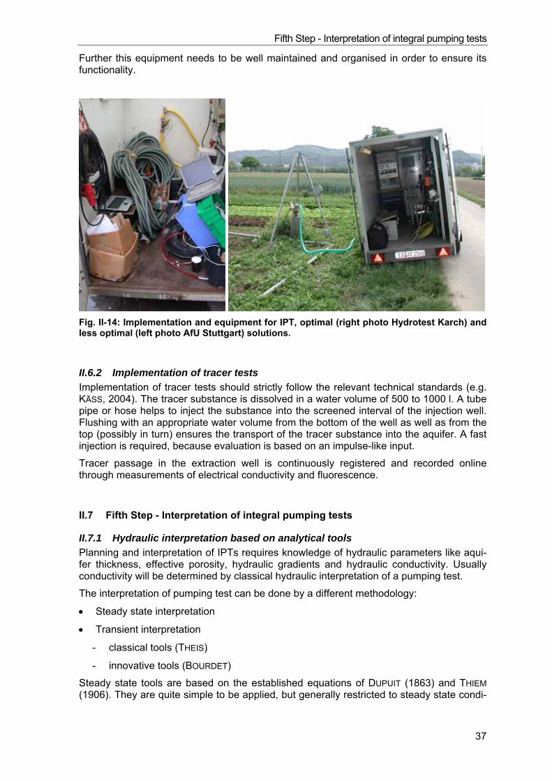
Fifth Step - Interpretation of integral pumping tests
37
Further this equipment needs to be well maintained and organised in order to ensure its functionality.
Fig. II-14: Implementation and equipment for IPT, optimal (right photo Hydrotest Karch) and less optimal (left photo AfU Stuttgart) solutions.
II.6.2 Implementation of tracer tests Implementation of tracer tests should strictly follow the relevant technical standards (e.g. KÄSS, 2004). The tracer substance is dissolved in a water volume of 500 to 1000 l. A tube pipe or hose helps to inject the substance into the screened interval of the injection well. Flushing with an appropriate water volume from the bottom of the well as well as from the top (possibly in turn) ensures the transport of the tracer substance into the aquifer. A fast injection is required, because evaluation is based on an impulse-like input.
Tracer passage in the extraction well is continuously registered and recorded online through measurements of electrical conductivity and fluorescence.
II.7 Fifth Step - Interpretation of integral pumping tests
II.7.1 Hydraulic interpretation based on analytical tools Planning and interpretation of IPTs requires knowledge of hydraulic parameters like aqui-fer thickness, effective porosity, hydraulic gradients and hydraulic conductivity. Usually conductivity will be determined by classical hydraulic interpretation of a pumping test.
The interpretation of pumping test can be done by a different methodology:
• Steady state interpretation
• Transient interpretation
- classical tools (THEIS)
- innovative tools (BOURDET)
Steady state tools are based on the established equations of DUPUIT (1863) and THIEM (1906). They are quite simple to be applied, but generally restricted to steady state condi-

Fifth Step - Interpretation of integral pumping tests
38
tions. They do not provide information about hydraulic boundaries and contain parameters which cannot exactly be defined (width of drawdown).
THEIS (1935) introduced transient interpretation of pumping tests, based on the temporal development of the drawdown in a confined aquifer. The conductivity can be defined graphically with the help of type curves, which are plotted together with the measurement data of the hydraulic heads in double logarithmic scale (curve-matching procedure).
COOPER & JACOB (1946) simplified the so called THEIS equation, as they recognised that in case of simple logarithmic plotting the temporal development of the hydraulic heads is following (after a short time of pumping) a logarithmic straight line. The slope can be used to calculate the conductivity (straight-line-method).
Other type curves were developed based on the THEIS-function, which allowed the appli-cation also in cases of hydraulic boundaries or semi-confined conditions (e.g. HANTUSH & JACOB 1955). However the general restriction of the THEIS method remains, no well-specific conditions like wellbore storage or well losses (skin) can be defined. But both are relevant phenomena which have to be considered in the interpretation of a pumping test, because in many cases only drawdown data from the extraction well are available and no further observation well or monitoring well can be measured. PAPADOPOLUS & COOPER (1967) introduced a solution for wells with large diameter, which was able to consider wellbore storage adequately.
In daily practice of consultancy pumping test interpretation is in most cases restricted to the previously mentioned standard methods. However the information gained by and based on these interpretations is by far not sufficient input to a proper interpretation of integral pumping tests. Numerous interpretation models were introduced within the last 35 years, which allow a much more precise quantification of the parameters and what is even more important, they enable an aquifer diagnosis, a profound characterisation of the boundary conditions and key features of the aquifer properties. Due to lacking awareness of these methods among practitioners they shall be subsequently described
In the 70s and 80s of the 20th century numerous new models for interpretation of pumping tests were developed mainly from the petroleum industry, which allow the application in a broad range of well and aquifer conditions. The new tools consider as an important factor the temporal derivative of the drawdown, which was introduced by BOURDET et al. (1983) for wells with wellbore storage and skin. In this case the temporal development of pres-sure data is plotted together with their derivative in a double logarithmic scale (“diagnostic plot”). As different flow regimes during a pumping test show significant differences in the slope of derivative, this method allows a much simpler identification of the radial flow re-gime (“THEIS–period”), for which the conductivity is to be defined. Changes of flow re-gimes can be detected and clearly defined, which allows a proper characterisation of hy-draulic properties of the aquifer (e.g. double porosity, single fracture response, hydraulic boundaries). Many of the currently available IT-programs for pumping test interpretation do offer the possibility of calculating pressure derivative.

Fifth Step - Interpretation of integral pumping tests
39
1. 10. 100. 1000. 1.0E+40.01
0.1
1.
10.
WellboreStorage
PressureDerivative
THEIS-typecurve
MB4 - Bleiglanzbank
Time [sec]
Infinite acting radial flow
Dra
wd
own
[m]
PAPADOPULOS & COOPER
Fig. II-15: Interpretation of pumping test with graphical representation of the derivative
Fig. II-15 shows an example for the hydraulic interpretation of a pumping test performed in the so called Bleiglanzbank of the MAGIC well MB4 in Stuttgart-Feuerbach. The fitting of the hydraulic test data was done according the solution of PAPADOPOULUS & COOPER for wells with wellbore storage and skin (see blue line). The red line shows the derivative of the type curve following the derivative drawdown data. The shape of the derivative with its typical hump shows, that the early time range is dominated by wellbore storage (slope about 1). After about 100 seconds of pumping the radial flow period begins to establish, which can be seen at the horizontal direction of the derivative (slope 0). Both the THEIS-type curve and the solution of PAPADOPOULUS & COOPER show identical curves after the effect of wellbore storage has finished.
The following table gives typical interpretation models for different flow periods.
Table II-5: Flow regimes during a pumping test and related models of interpretation (modi-fied acc. to BOURDET, 2002)
Regime of flow
Slope of deriva-tive
Interpretation model
(log-log-scale) early time range
intermediate time range
late time range
Radial 0 (= 0°) Double porosity (restricted)
Homogeneous behaviour
(THEIS-period)
Semi-infinite reservoir

Fifth Step - Interpretation of integral pumping tests
40
Regime of flow
Slope of deriva-tive
Interpretation model
(log-log-scale) early time range
intermediate time range
late time range
Linear
0.5 (= 22.5°) Infinite conduc-tivity fracture
Horizontal well Two parallel no flow boundaries
(trench)
Bi-linear 0.25 (= 11.25°) Finite conductivity
fracture
Finite conductiv-ity
fault
Spherical
-0.5 (= -22.5°) Partially pene-trating well
Pseudo steady state
1 (= 45°) Wellbore stor-age
Closed reservoir
Steady state -1 (= -45°) Conductive fault Constant pres-sure boundary,
leakage Besides a reliable determination of the hydraulic conductivity it is essential for the interpretation of an IPT to identify hydraulic boundaries (no flow and constant pressure) as well as vertical connections (leakage) and exchange processes with surface waters. In case of active recharge into the pumped aquifer the width of the capture zone after a defined time is smaller compared to the case of an unbounded THEIS-aquifer. In this case the width of capture zone calculated according to BEAR & JACOBS (1965) would be overestimated. Accordingly it is important to detect leaky boundaries and to consider them in the numerical interpretation of the IPT.
Transmissivities obtained by the hydraulic interpretation of IPTs in many cases will be different to those transmissivities which were used for the design of the IPT. This is due to the fact, that data used for the design in most cases originate from previously performed short term pumping tests. These short term tests only characterise a very narrow area around the extraction wells due to the short pumping time, which gives only very local hydraulic information. An IPT which runs over several days characterises a much larger area of the aquifer, delivering much better regional average data. The effects of incidental small scale heterogeneities are compensated with increasing pumping time, as demon-strated in Fig. II-16.

Fifth Step - Interpretation of integral pumping tests
41
Tran
smis
sivi
ty (
m/s
)2
10-1
10-2
10-3
10-4
10-5
10-6
10-7
0 250 500 750 1000 1250 1500
Pumping time (h)
Middle Keuper (Bochinger Horizont, Dunkelrote Mergel)
Fig. II-16: Relationship between time of pumping and resulting transmissivity (UFRECHT, un-published)
II.7.2 Interpretation of tracer tests The interpretation of tracer tests is to be done with the equation introduced of SAUTY as mentioned in chapter II.5.4. The tool for design and interpretation can be used to setup a graphical representation with a concentration curve representing the mass of the tracer recovered. Input data are the distance to the injection well of the tracer, thickness of the aquifer, pumping rate, and the mass of the tracer injected. When calculating the concen-tration curve the values for effective porosity and dispersivity could be manually varied until the calculated curve fits well to the measured curve.
Design and Interpretation Tool Tracer Test
Test records IGWM 9pumping rate m³/s 0,005aquifer thickness m 3,3distance m 13,5tracer NaClmass kg 20time of tracer input 16.06.2004 11:15recovery rate % 72,0% limit of detectiondetection limit µS/cm 10 0 890background concentr µS/cm 880 25,00 890
Transport parameterne 0,10alphaL m 2,50
880
900
920
940
960
980
1000
1020
1040
0 5 10 15 20 25time [h]
elec
tric
cond
uctiv
ity [µ
S/cm
]
computed [µS/cm]measured [µS/cm]limit of detection
Fig. II-17: Example of the interpretation of a tracer test and determination of the transport parameters meαL by fitting of the calculated and actually measured concentration curves

Fifth Step - Interpretation of integral pumping tests
42
II.7.3 Contaminant specific interpretation MAGIC tool MAGIC software tool allows for interpretation of results of IPT in the case of pumping sin-gle wells at one time or no significant interference among simultaneously pumped wells. Results for each well are separately calculated and visualised in simple GIS environment.
Required input parameters are the same as for IPT planning plus the laboratory results for the given contaminant at each time step (Fig. II-18). The time steps are determined by sampling in such sense, that each groundwater sample is linked to one time step (Tx). In practice, the needed data are the time steps (represented by the hours since start of pumping) and the related concentrations of the contaminant measured in given time.
Fig. II-18: Inputting the laboratory result for each time step of IPT
The software then calculates the main IPT results (Fig. II-19). The main and very reliable results are:
• Contaminant mass flow rate across the control plane of individual well
• Average concentration of water flowing through the control plane
The software also gives the comparison between the concentration measured in the sam-ple and the calculated “real” concentration in the aquifer (evaluated taking into account the dilution effect due to pumping). It has to be stressed that the evaluated concentrations are to be considered as a rough estimate. Their calculation is based on assumptions with re-gard to the position of the plume in relation to the well. In some cases of high variability of concentration perpendicular to groundwater flow the evaluated concentrations for single streamtubes could even show negative values. If the negative values are single cases and they are low in magnitude, their presence should not confuse, as they are indicating high variability of concentrations. In these cases the peak concentration might be overesti-mated, but the contaminant mass flow and the average concentration are still very reliable (as values representing wider area of max. capture zone). Also the qualitative relationship between the distance from extraction well and the concentration (concentration pattern across the control plane) is a valuable information. Even if the magnitude of the maximum concentration might be not very precise (as it is very sensitive to even small parameter changes) the position of the peak concentration (centre of contaminant plume) can be considered reliable.

Fifth Step - Interpretation of integral pumping tests
43
Fig. II-19: Results of IPT evaluation using MAGIC software tool
Fig. II-20: Inputting simple GIS information
Based on very simple GIS information, such as position of the well and groundwater flow direction (Fig. II-20) the results can be visualised in GIS environment (Fig. II-21). The main visualised results are the isochrones of IPT (concentric ellipses), the width of control plane (represented by dark grey bar) and the expected centre of the plume (zone of peak concentration – shown as a violet stripe). The violet stripe can be displayed either on the left or on the right side of the extraction well, according to user’s decision based on site-specific information. The Software allows also for saving the generated graphics as a vec-tor file with the co-ordinates (in .SHP format). The results can also be exported to a report in spreadsheet format.

Fifth Step - Interpretation of integral pumping tests
44
Fig. II-21: GIS visualisation of IPT results with MAGIC software tool
The results of the MAGIC-site in Olsztyn (see Fig. II-22) demonstrate the quality of results obtained from the integral investigation at small scale. Based on the analytical interpreta-tion of the IPTs and combined with a simple numerical flow model several plumes of pollu-tion could be delineated and the related sources of pollution identified.
£yna River
£yna River
Existing old gasworks buildings
Buried old gas-container with tar remains (“barrow”)
Reconstructed localization of main production & gas-purification buildings
Hypothetical zone of contamination in classical approach
Control plane with boreholes for IPTCalculated pathway from source of pollution inMAGIC approach
A B
Groundwater flow direction
Fig. II-22: Old gasworks area in Olsztyn – comparison of results to be expected from classi-cal investigation (A) and detailed results received from the application of integral investiga-tion approach

Fifth Step - Interpretation of integral pumping tests
45
Further information is provided in MAGIC software manual available via:
www.magic-cadses.com
II.7.4 Numerical Interpretation
II.7.4.1 Basic principles The analytical tools described in the previous chapters were specifically developed for IPT – interpretation. They use the inversion of the transport equation to directly determine the relevant parameters.
Numerical interpretation means first to establish a complete numerical site model which will then be used to simulate the IPT. This simulation is always an iterative process, which means to receive the spatial distribution of the contaminants as a result of a flow and transport modelling in several steps.
II.7.4.2 Groundwater flow model As the numerical interpretation of IPT requires a site model the general demands on nu-merical modelling of groundwater flow and transport have to be met (see e.g. KINZELBACH et al., 1996; RAUSCH et al., 2005).
The hydrogeological model (see chapter II.4.) is fundamentally needed. It describes all relevant parameters of groundwater flow and contaminant transport. Most important are the structure of the aquifer, hydraulic properties and boundary conditions. Digital maps of the spatial distribution of the parameters should be available.
In a first step the flow model is built up and calibrated by an up to date representation of hydraulic heads. In cases with simple hydrogeological conditions combined with tight clus-ters of data a proper simulation of the hydraulic heads might be possible in a first attempt. However in most cases significant uncertainties will require further adjustment of the pa-rameters during the model calibration. Later the simulation if the IPT will additionally en-able a local fine-tuning of the calibration.
As contaminant transport in groundwater is mainly a long term process, in many cases a stationary calibration of the groundwater flow for average conditions is sufficient.
II.7.4.3 Transport model A calibrated groundwater flow model is prerequisite for the simulation of the transport processes, which should in a first step describe the regional contaminant distribution. This could be done by implementing first potentially contaminated sites and contaminant source zones already known. Based on this information the contaminant transport can be calculated as long as a quasi-stationary spatial distribution of contaminants will be achieved. This will be finally calibrated by a simultaneous reference sampling and analysis campaign of all wells. This procedure is recommended if the contamination is much older than the residence time of the particles within the model area. In cases of young contami-nations quasi-stationary conditions cannot be presumed, which requires transient simula-tion. Calculated contaminant distributions can be used as starting position or initial con-centrations for the simulation of the IPT.
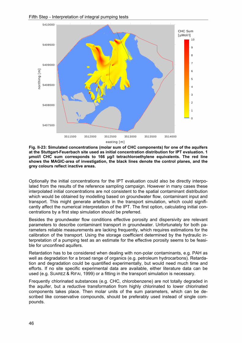
Fifth Step - Interpretation of integral pumping tests
46
3511500 3512000 3512500 3513000 3513500 3514000
easting [m]
5407500
5408000
5408500
5409000
5409500
5410000
nort
hing
[m
]
0
1
2
3
4
5
6
7
8
9
10
CHC Sum[µMol/l]
Fig. II-23: Simulated concentrations (molar sum of CHC components) for one of the aquifers at the Stuttgart-Feuerbach site used as initial concentration distribution for IPT evaluation. 1 µmol/l CHC sum corresponds to 166 µg/l tetrachloroethylene equivalents. The red line shows the MAGIC-area of investigation, the black lines denote the control planes, and the grey colours reflect inactive areas.
Optionally the initial concentrations for the IPT evaluation could also be directly interpo-lated from the results of the reference sampling campaign. However in many cases these interpolated initial concentrations are not consistent to the spatial contaminant distribution which would be obtained by modelling based on groundwater flow, contaminant input and transport. This might generate artefacts in the transport simulation, which could signifi-cantly affect the numerical interpretation of the IPT. The first option, calculating initial con-centrations by a first step simulation should be preferred.
Besides the groundwater flow conditions effective porosity and dispersivity are relevant parameters to describe contaminant transport in groundwater. Unfortunately for both pa-rameters reliable measurements are lacking frequently, which requires estimations for the calibration of the transport. Using the storage coefficient determined by the hydraulic in-terpretation of a pumping test as an estimate for the effective porosity seems to be feasi-ble for unconfined aquifers.
Retardation has to be considered when dealing with non-polar contaminants, e.g. PAH as well as degradation for a broad range of organics (e.g. petroleum hydrocarbons). Retarda-tion and degradation could be quantified experimentally, but would need much time and efforts. If no site specific experimental data are available, either literature data can be used (e.g. SUAREZ & RIFAI, 1999) or a fitting in the transport simulation is necessary.
Frequently chlorinated substances (e.g. CHC, chlorobenzene) are not totally degraded in the aquifer, but a reductive transformation from highly chlorinated to lower chlorinated components takes place. Then molar units of the sum parameters, which can be de-scribed like conservative compounds, should be preferably used instead of single com-pounds.
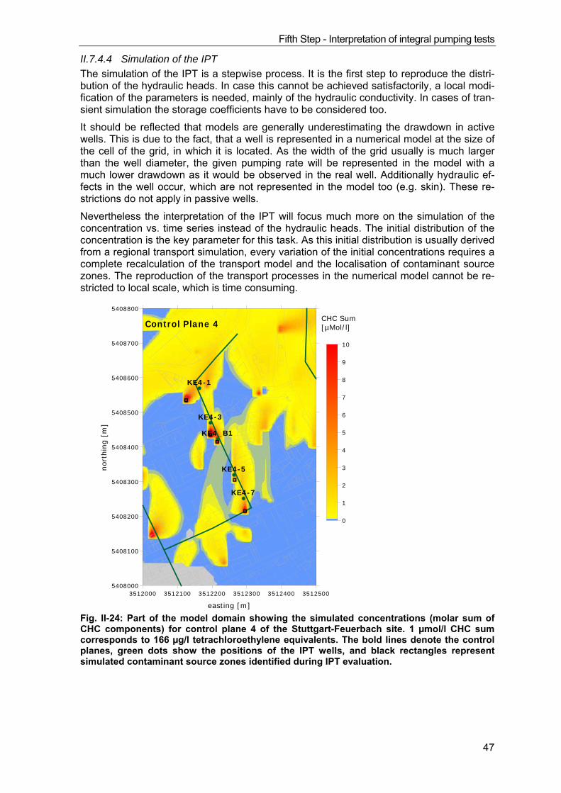
Fifth Step - Interpretation of integral pumping tests
47
II.7.4.4 Simulation of the IPT The simulation of the IPT is a stepwise process. It is the first step to reproduce the distri-bution of the hydraulic heads. In case this cannot be achieved satisfactorily, a local modi-fication of the parameters is needed, mainly of the hydraulic conductivity. In cases of tran-sient simulation the storage coefficients have to be considered too.
It should be reflected that models are generally underestimating the drawdown in active wells. This is due to the fact, that a well is represented in a numerical model at the size of the cell of the grid, in which it is located. As the width of the grid usually is much larger than the well diameter, the given pumping rate will be represented in the model with a much lower drawdown as it would be observed in the real well. Additionally hydraulic ef-fects in the well occur, which are not represented in the model too (e.g. skin). These re-strictions do not apply in passive wells.
Nevertheless the interpretation of the IPT will focus much more on the simulation of the concentration vs. time series instead of the hydraulic heads. The initial distribution of the concentration is the key parameter for this task. As this initial distribution is usually derived from a regional transport simulation, every variation of the initial concentrations requires a complete recalculation of the transport model and the localisation of contaminant source zones. The reproduction of the transport processes in the numerical model cannot be re-stricted to local scale, which is time consuming.
3512000 3512100 3512200 3512300 3512400 3512500
easting [m]
5408000
5408100
5408200
5408300
5408400
5408500
5408600
5408700
5408800
nort
hing
[m
]
KE4-1
KE4-3
KE4-5
KE4-7
KE4_B1
0
1
2
3
4
5
6
7
8
9
10
CHC Sum[µMol/l]Control Plane 4
Fig. II-24: Part of the model domain showing the simulated concentrations (molar sum of CHC components) for control plane 4 of the Stuttgart-Feuerbach site. 1 µmol/l CHC sum corresponds to 166 µg/l tetrachloroethylene equivalents. The bold lines denote the control planes, green dots show the positions of the IPT wells, and black rectangles represent simulated contaminant source zones identified during IPT evaluation.
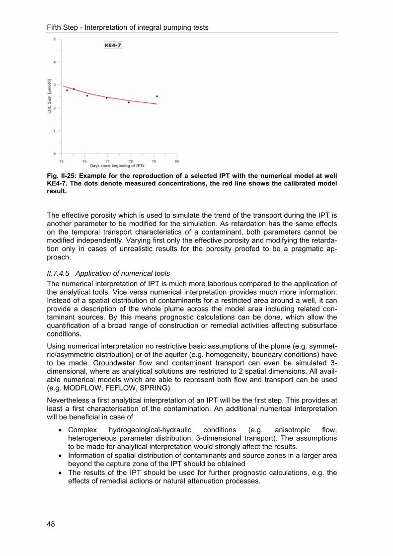
Fifth Step - Interpretation of integral pumping tests
48
Fig. II-25: Example for the reproduction of a selected IPT with the numerical model at well KE4-7. The dots denote measured concentrations, the red line shows the calibrated model result.
The effective porosity which is used to simulate the trend of the transport during the IPT is another parameter to be modified for the simulation. As retardation has the same effects on the temporal transport characteristics of a contaminant, both parameters cannot be modified independently. Varying first only the effective porosity and modifying the retarda-tion only in cases of unrealistic results for the porosity proofed to be a pragmatic ap-proach.
II.7.4.5 Application of numerical tools The numerical interpretation of IPT is much more laborious compared to the application of the analytical tools. Vice versa numerical interpretation provides much more information. Instead of a spatial distribution of contaminants for a restricted area around a well, it can provide a description of the whole plume across the model area including related con-taminant sources. By this means prognostic calculations can be done, which allow the quantification of a broad range of construction or remedial activities affecting subsurface conditions.
Using numerical interpretation no restrictive basic assumptions of the plume (e.g. symmet-ric/asymmetric distribution) or of the aquifer (e.g. homogeneity, boundary conditions) have to be made. Groundwater flow and contaminant transport can even be simulated 3-dimensional, where as analytical solutions are restricted to 2 spatial dimensions. All avail-able numerical models which are able to represent both flow and transport can be used (e.g. MODFLOW, FEFLOW, SPRING).
Nevertheless a first analytical interpretation of an IPT will be the first step. This provides at least a first characterisation of the contamination. An additional numerical interpretation will be beneficial in case of
• Complex hydrogeological-hydraulic conditions (e.g. anisotropic flow, heterogeneous parameter distribution, 3-dimensional transport). The assumptions to be made for analytical interpretation would strongly affect the results.
• Information of spatial distribution of contaminants and source zones in a larger area beyond the capture zone of the IPT should be obtained
• The results of the IPT should be used for further prognostic calculations, e.g. the effects of remedial actions or natural attenuation processes.

Fifth Step - Interpretation of integral pumping tests
49
Basically the intention to use numerical interpretation does not require special design or implementation of the IPT. But for the calibration of the model representative simultane-ous measurements of hydraulic heads and concentration covering the whole model area are needed. These data should be acquired before the start of the IPT.
II.7.5 Other available tools
II.7.5.1 Basic Principle In ideal cases of homogeneous, isotropic confined aquifers the interpretation can be done by analytical solution. The analytical solution without consideration of the basic flow can be described according to SCHWARZ (2002):
E is to be defined as the mass flow rate in the control plane and ci the contaminant con-centration at the time ti.
ĉ is the mean concentration of two stream tubes at left and right side of the extraction well in the distance r.
The formula:
represents the natural flow regime in both stream tubes perpendicular to the control plane and ri = √Qt / πbnp the radius of the isochrone at time ti, Q representing the pumping rate. The variant b represents the aquifer thickness, np the effective porosity and n the total number of concentration measurements used for the curve. For the first time interval ĉ1 = c1. For further details see BOCKELMANN et al. 2001.
II.7.5.2 Simplified analytical solution With the help of an Excel – based IPT tool developed by ROTHSCHINK-UW integral pump-ing test can be planned and interpreted on an analytical basis (ROTHSCHINK, 2007).
Bases on the results of the chemical analysis of the groundwater samples of an IPT those contaminant concentrations of the groundwater are calculated, which theoretically have to be assumed to generate the concentrations measured. Each sample represents the aver-age concentration for the respective isochrone at the given sampling time. The calculation of mass flow rates [g/d] across a control plane perpendicular to the groundwater flow di-rection which is covered by an IPT, requires besides the calculation of mean contaminant concentrations [µg/l] the related mass flow [m3/d] of groundwater too.
The simplified calculation according to BEAR & JACOBS and the evaluation of the “theoreti-cal” concentrations is based on following assumptions:
1) Initially parallel groundwater flow in the whole area covered by the IPT
2) no gradients of concentration in direction of groundwater flow
3) gradients of contaminant concentration perpendicular to groundwater flow direc-tion
4) radial symmetric isochrones at sampling times
The following examples illustrate the results, which can be obtained by this Excel based tool.

Fifth Step - Interpretation of integral pumping tests
50
The first example shows a pumping test in a well located about 6m besides a plume of CHC. To explain a CHC-concentration of 12.1 µg/l in the last sample requires a plume which actually shows about 40-50 (calculated 48) µg/l CHC in about 14-15m distance to the extraction well. In the second example the integral pumping test completely covers a narrow benzene plume, with a concentration maximum about 60-70 µg/l in about 5.7 m distance to the well. The final example with the PAH demonstrates an IPT with the highest contaminant concentration on the first sample. This indicates a position of the extraction well in the center of a plume which leads to decreasing concentration in the following pumping phase. The calculation further exhibits that the edge of the plume is nearly de-tected by the IPT although the last samples still ranging between 180-190 µg/l.
CHC
0 10 20 30 40 50 60
0 2 4 6 8 10 12 14 16Distance to extraction well [m]
[µg/
l]
Benzene
0 10 20 30 40 50 60 70 80
0 2 4 6 8 10 12 14 16 Distance to extraction well [m]
[µg/
l]
Analytical result: average conc. of isochrones [µg/l] Calculated conc. for groundwater at tx [µg/l]
PAH 15
0 50
100 150 200 250 300 350
0 2 4 6 8 10 12 14 16Distance to extraction well [m]
[µg/
l]
Analytical result: average conc. of isochrones [µg/l] Calculated conc. for groundwater at tx [µg/l]
Analytical result: average conc. of isochrones [µg/l] Calculated conc. for groundwater at tx [µg/l]
Fig. II-26: Concentrations vs. distance to extraction well showing concentrations measured and calculated

Fifth Step - Interpretation of integral pumping tests
51
Table II-6: Mass flow rates and mean concentrations (ROTHSCHINK, unpublished)
CHC Benzene PAH 15 Analysis: mixture of isochrone samples [µg/l]
Onsided: Calcul. for GW section tx [µg/l]
Analysis: mixture of isochrone samples [µg/l]
Onsided: Calcul. for GW section tx [µg/l]
Analysis: mixture of isochrone samples [µg/l]
Onsided: Calcul. for GW section tx [µg/l]
2 2.0 324 324.0 5 8.0 295 266.0 12 31.1 254 130.7 23 68.2 231 75.4
0.8 3.6 25 62.9 214 34.6 2.1 8.9 23 45.5 205 26.5 4.3 18.5 19 24.0 198 16.0 6.4 26.0 15 7.4 192 4.7 9.4 38.9 13 5.4 188 2.2
12.1 48.0 11 0.1 185 0.8 R-Concentr [µg/l]
7.19 R-Concentr. [µg/l]
13.73 R-Concentr. [µg/l]
206.05
Flow rate [m³/d]
61.7 Flow rate [m³/d]
61.7 Flow rate [m³/d]
61.7
Mass flow [g/d]
0.44 Mass flow [g/d]
0.85 Mass flow [g/d]
12.71
II.7.5.3 Analytical-numerical solution (CSTREAM) The simulation tool CSTREAM (BAYER-RAICH) can be classified as in an intermediate be-tween the analytical tools and the numerical tools described in chapter II.7.4. In July 2006 a tutorial took place in the Center for Applied Geology of University Tübingen dealing with integral pumping tests and the evaluation software CSTREAM, which is since then avail-able from the Tübingen group.
CSTREAM is based on the analytical solution of the transport equation. This is why it is described in this chapter about analytical tools. Compared to the other tools described so far it is additionally able to use a numerical solution to describe the groundwater flow. This can be done using the well known flow model MODFLOW (MCDONALD & HARBAUGH, 1988) and the pathline module MODPATH (POLLOCK, 1994), which are incorporated in CSTREAM. This enables the consideration of heterogeneous groundwater flow too. Until now, the numerical flow model is restricted to 2 spatial dimensions.
Significant efforts are needed to apply the numerical option for groundwater flow in CSTREAM, as this requires to set-up a groundwater flow model for the site. Nevertheless these efforts are less compared to the fully numerical interpretation as described in chap-ter II.7.4., as no calibration of the regional transport model in necessary.
As the previously described tools CSTREAM generates spatial distribution of contami-nants and their characteristic parameters restricted to the capture zone of the IPT. As no numerical simulation of the contaminant transport is included, further information about e.g. total plume length, contaminant source zones and transport prognosis cannot be generated directly.

Glossary
52
GLOSSARY
English German Polish Czech
according to its best judgment
nach pflichtgemä-ßem Ermessen
zgodnie z najlepszą oceną
podle nejlepšího úsudku
approach Strategie podejście, metodyka přístup řešení
aquifer Grundwasserleiter warstwa wodonośna (wodonosiec)
hydrogeologický kolektor (zvodeň)
backtracking Rückverfolgung śledzenie wsteczne backtracking (vyhle-dání zdroje inverzní metodou (numeri-ckou, analytickou)
body of groundwater Grundwasserkörper jednolite części wód podziemnych (jcwp)
podzemní voda v daném hydrogeologickém kolektoru
breach of law (regularity offence)
Rechtsverletzung złamanie/naruszenie prawa
porušení zákona
breach of the public safety
Störung der öffentli-chen Sicherheit und Ordnung
Naruszenie bezpieczeństwa publicznego
obecné ohrožení
case by case ap-proach
Einzelfallbearbeitung Podejście zindywidualizowane
přístup založený na řešení jednotlivých zdrojů znečištění bez návaznosti na sousedící zdroje
competent authority zuständige Behörde władza/instytucja właściwa do spraw
odpovědný správní orgán
contaminant mass flow rate
Schadstofffracht przepływ masy substancji zanieczyszczającej
emisní tok škodliviny
control plane Kontrollebene przekrój badawczy kontrolní profil
defined pollution punktförmiger Schadstoffeintrag
Rozpoznane zanieczyszczenie
definované znečiš-tění
emission rate Quellstärke wielkość emisji velikost emisního toku
entry of pollutants Schadstoffeintrag wprowadzanie substancji zanieczyszczających
vstup škodlivin do prostředí
environmental damage
Umweltschaden Szkoda środowiskowa
škoda na životním prostředí
environmental protection authority
Umweltbehörde organ właściwy d.s. ochrony środowiska
správní orgán činný v ochraně životního prostředí

Glossary
53
English German Polish Czech
fingerprinting/ fingerprints
Fingerabdruck zur Schadstoffcharakte-risierung, z. B. durch Analyse des Chro-matogramms
szczegółowe badania izotopowe, także z ang. fingerprinting
otisk (metoda průzkumu využivající charakteristického znaku šetřeného problému – např. použití stopovače při určení dráhy postupu znečištění)
groundwater flow direction
Grundwasserfließ-richtung
kierunek przepływu wód podziemnych
směr proudění podzemní vody
Groundwater investigation
Grundwasserunter-suchung
badanie wód podziemnych
průzkum znečištění podzemních vod
Groundwater pollution
Grundwasserverun-reinigung
zanieczyszczenie wód podziemnych
znečištění podzemní vody
groundwater reatment
Grundwasserbe-handlung
1. remediacja wód podziemnych; 2. postępowanie z zanieczyszczonymi wodami podziemnymi
nákladání se znečištěnými podzemními vodami
integral pumping test Immisionspumpver-such
Immisyjne pompowanie badawcze/testowe (IPT)
integrální čerpací zkoušky
leachate Sickerwasser odciek výluh
liability Verantwortlichkeit odpowiedzialność odpovědnost
monitoring Beobachtung, Über-wachung
monitoring monitoring
natural retention and degradation, modification processes (Natural Attenuation)
natürliche Rückhal-te-, Abbau- oder Umwandlungsvor-gänge (Natural Atte-nuation)
naturalna retencja i degradacja substancji, modyfikacja procesów retencji i degradacji (samooczyszczanie)
procesy přirozené atenuace
objective (e.g. of treatment)
Ziel (z.B. Behand-lungsziel)
cel (np. remediacji) cíl (např. naprávných opatření)
official identification of liable persons
Amtsermittlung wskazanie z urzędu sprawcy
úřední ustanovení odpovědné osoby
owner liability (owner liable for a danger-ous good/condition)
Zustandsstörer-Haftung
odpowiedzialność władającego (władający odpowiedzialny za dobry/zły stan)
odpovědnost vlastníka nemovitosti
pathway Transportweg droga migracji dráha postupu (např. znečištění) prostředím

Glossary
54
English German Polish Czech
plume of pollution Schadstofffahne smuga zanieczyszczenia
kontaminační mrak
pollutant load, pollutant charge
Schadstofffracht ładunek substancji zanieczyszczającej
zatížení škodlivinou (např. prostředí)
pollutant phase body Schadstoff-Phasenkörper
faza substancji zanieczyszczającej
škodlivina ve fázi
polluter Verursacher (eines Schadens)
sprawca zanieczyszczenia
původce znečištění
polluter liability (pol-luter: someone who endangers the public by his/her actions)
Handlungsstörerhaf-tung, Verursacher-haftung
odpowiedzialność sprawcy zanieczyszczenia
odpovědnost původce znečištění
significant and sustained upward trend in concentrations of pollutants
signifikanter und anhaltender Trend der Zunahme von Schadstoffkonzent-rationen
znaczący i trwały trend wzrostu stężeń substancji zanieczyszczających
významný a stále se zvyšující nárůst koncentrací škodlivin
site, location Standort teren, obiekt, lokalizacja
lokalita
source of pollution Schadensherd źródło zanieczyszczenia, ognisko zanieczyszczenia
zdroj znečištění
subject of protection Schutzgut przedmiot ochrony předmět ochrany
tracing Nachverfolgung trasowa-nie/wyznaczanie trasy
stopování/sledování
treatment of sources of pollution
Schadensherdbear-beitung
postępowanie ze źródłami/ogniskami zanieczyszczenia
nápravné opatření k odstranění zdroje znečištění
trend reversal Trendumkehr odwrócenie trendu obrácený vývoj

References
55
REFERENCES
BAUER, S., BAYER-RAICH, M, HOLDER, T., KOLESAR, CH., MÜLLER, D. & PTAK, T. (2004): Quantification of groundwater contamination in an urban area using inte-gral pumping tests, Journal of Hydrology, 75, 183.
BAYER-RAICH, M. (2004): Integral pumping tests for the characterization of groundwater contamination, Ph.D. Thesis, Center for Applied Geoscience, University of Tü-bingen.
BAYER-RAICH, M., BAUMANN, R. & PTAK, T. (2002): Estimation of contaminant mass flows in a multi-layered aquifer using pumping tests: numerical experiments at field scale. In: Groundwater Quality: Natural and Enhanced Restoration of Groundwater Pollution, THORNTON, S.F. & OSWALD S.E. (Hrsg.) IAHS Publication No. 275.
BAYER-RAICH, M., JARSJÖ, J., HOLDER, T. & PTAK, T. (2003): Numerical Estimations of contaminant concentration and mass flow in aquifers from time dependent pumping wells. Model Care 2002: A Few Steps Closer to Reality, IAHS Publica-tion No. 277.
BAYER-RAICH, M., JARSJÖ, J., LIEDL, R., PTAK, T. TEUTSCH, G. (2004): Average contaminant concentration and mass flow in aquifers from time dependent pump-ing well data: analytical framework, Water Resour. Res., 40.
BEAR, J. & JACOBS, M. (1965): On the movement of waterbodies injected into aquifers. – Journ. Hydrol. 3 (1), S. 37 – 57.
BEER, H.-P., KIEFER, R., HOLDER, T. & PTAK, T (2002): Grundwasserabstromerkun-dung durch Immissionsmessung. – Stand der Technik, Planung, Implementie-rung. Schriftenreihe Altlastenforum Baden-Württemberg e.V., Heft 8.
BLÜMLING, P. & HUFSCHMIED, P. (1989): Fluid-Logging in Tiefbohrungen. Nagra infor-miert, S. 24-38, 3+4/89, Baden (Schweiz).
BOCKELMANN, A., PTAK, T. & TEUTSCH, G. (2002): An analytical quantification of mass fluxes and natural attenuation rate constants at a former gasworks site. J. Contam. Hydrol., 53(3-4), ISSN 0169-7722.
BOURDET, D. (2002): Well test analysis: the use of advanced interpretation models. – Elsevier.
BOURDET, D., WHITTLE, T.M., DOUGLAS, A.A. & PIRARD, Y.M. (1983): A new set of type curves simplifies well test analysis. – World Oil, May, S. 95 – 106, Gulf Pub-lishing Co.
COOPER, H.H. & JACOB, C.E. (1946): A generalized graphical method for evaluation formation constants and summarizing well-field-history. Trans. Am. Geoph. Union 27, S. 526 – 534.
DUPUIT, J. (1863): Etudes théoriques et pratiques sur le mouvement des eaux dans les canaux découverts et à travers les terrains perméables. 2. Aufl., 304 S.
FH-DGG (1999): Hydrogeologische Modelle – Ein Leitfaden für Auftraggeber, Ingenieur-büros und Fachbehörden. – Schriftenreihe der Deutschen Geologischen Gesell-schaft, 10, 36 S.
FH-DGG (2002 a): Das Hydrogeologische Modell als Basis für die Bewertung von Monito-red Natural Attenuation bei der Altlastenbearbeitung. Ein Leitfaden für Auftragge-ber, Ingenieurbüros und Fachbehörden. – Schriftenreihe der Deutschen Geologi-schen Gesellschaft, 23: 29 S.
FH-DGG (2002 b): Hydrogeologische Modelle – Ein Leitfaden mit Fallbeispielen. – Schrif-tenreihe der Deutschen Geologischen Gesellschaft, 24: 120 S.

References
56
HANTUSH, M.S. & JACOB, C.E. (1955): Non-steady radial flow in an infinite leaky aqui-fer. – Trans. Am. Geoph. Union 36, S. 95 – 100.
HOLDER, T. & TEUTSCH, G. (1999): Prinzip des neuen Immissionsmessverfahrens, An-wendung der Immissionsmessung im Neckartal; in: Integrale Altlastenerkundung im Stuttgarter Neckartal, Schriftenreihe des Amtes für Umweltschutz, 4/1999, Stuttgart.
HOLDER, T., TEUTSCH, G., PTAK T. & SCHWARZ, R. (1998): A new approach for source zone characterization: the Neckar Valley study. In Groundwater Quality: Remediation and Protection, IAHS Publication No. 250, ISSN 0144-7815, 49-55.
INCORE (2003): Integrated Concept for Groundwater Remediation INCORE – final report. – Stuttgart, 26 P.
INGEGNERIA E GEOLOGIA DEGLI ACQUIFERI – IGEA (2004): N. 19-2004 - Special Issue on the INCORE project.- Torino, 109 P.
ISO 5667-1:WATER QUALITY. SAMPLING. PART 1: GUIDANCE ON THE DESIGN OF SAMPLING PROGRAMMES, CEN 1980.
ISO 5667-2: WATER QUALITY. SAMPLING. PART 2: GUIDANCE ON SAMPLING TECHNIQUES CEN 1991.
ISO 5667-3: WATER QUALITY. SAMPLING. PART 3: GUIDANCE ON THE PRESERVATION AND HANDLING OF WATER SAMPLES CEN 2003.
JARSJÖ, J., PTAK, T., BAYER-RAICH, M. & HOLDER, T. (2002): Uncertainties in con-taminant plume characterisations based on concentration measurements in pum-ping wells: The Stuttgart-Neckartalaue site. Paper for the 4th International Confe-rence on Calibration and Reliability in Groundwater Modelling, Prague, Czech Republic, 17-20 June 2002.
KÄSS, W. (2004): Geohydrologische Markierungstechnik - 2. überarbeitete Aufl., 557 Sei-ten, 239 Abbildungen, 43 Tabellen, 8 Farbtaf. (Lehrbuch der Hydrogeologie, Band 9).
KINZELBACH, W., VOSS, A., RAUSCH, R., SAUTY, J.-P., CHIANG, W.H., CORDES, C. & FANG, S. Z. (1996). Berechnungsverfahren und Modelle, in Altlastenhandbuch des Landes Niedersachsen, Materialenband, Niedersächsisches Landesamt für Ökologie, Hildesheim und Niedersächsisches Landesamt f. Bodenforschung, Hannover, Springer Verlag Berlin, Heidelberg, New York, 216 S., 163 Abb., 11 Tab., CD-ROM.
LANDESHAUPTSTADT STUTTGART – AMT FÜR UMWELTSCHUTZ (1999): Kalibrie-rung eines regionalen Grundwasserströmungsmodells mit Hilfe von Umweltisoto-peninformationen. - Schriftenreihe des Amtes für Umweltschutz – Heft 1/1999. Stuttgart, 160 S.
LANDESHAUPTSTADT STUTTGART – AMT FÜR UMWELTSCHUTZ (1999): Integrale Altlastenerkundung im Neckartal Stuttgart. - Schriftenreihe des Amtes für Um-weltschutz – Heft 4/1999. Stuttgart, 192 S.
LANDESHAUPTSTADT STUTTGART – AMT FÜR UMWELTSCHUTZ (2001): Integriertes Konzept zur Grundwassersanierung INCORE – [Integrated Concept for Ground-water Remediation]. Stuttgart, 23 S.
LANDESHAUPTSTADT STUTTGART – AMT FÜR UMWELTSCHUTZ (2003): Kommuna-ler Umweltbericht: Das Grundwasser in Stuttgart. - Schriftenreihe des Amtes für Umweltschutz – Heft 1/2003. Stuttgart, 202 S.

References
57
LANDESHAUPTSTADT STUTTGART – AMT FÜR UMWELTSCHUTZ (2006): Hydrogeo-logie des Stuttgarter Mineralwassersystems. – Schriftenreihe des Amtes für Um-weltschutz – Heft 3/2006. Stuttgart, 152 S.
MCDONALD, M. & HARBAUGH, W., 1988. MODFLOW – A Modular 3-dimensional Finite-Difference Groundwater Flow Model. – U. S. Geological Survey, 1988.
MOENCH, A.F. (1985): Transient flow to a large-diameter well in an aquifer with storative semiconfining layers. – Water Resources Research, Vol. 21, No. 8, S. 1121 – 1131.
PAPADOPULOS, I.S. & COOPER, H.H. (1967): Drawdown in a well of large diameter. – Water Resources Research, Vol. 3, S. 241 – 244.
POLLOCK, D.W., 1994. User’s Guide for MODPATH/MODPATH-PLOT, Version 3: A par-ticle tracking post-processing package for MODFLOW, the U.S. Geological Sur-vey finite-difference ground-water flow model: U.S. Geological Survey, 1994.
PTAK, T. & TEUTSCH, G. (1997): Grundwasser-Gefährdungsabschätzung durch Emissi-ons- und Immissionsmessungen an Deponien und Altlasten - Numerische Unter-suchungen zur Anwendung und Auswertung, Projekt Wasser-Abfall-Boden PWAB, Projekt-Nr.: PD 96 181, Bericht, Lehrstuhl für Angewandte Geologie der Universität Tübingen.
PTAK, T. & TEUTSCH, G. (2000): Development and application of an integral investiga-tion method for the characterization of groundwater contamination. – Contami-nated Soil 2000.
PTAK, T., BAYER-RAICH, M. BAUER, S. (2004): Tiefenorientierte integrale Erkundung der Schadstoffbelastung in großräumig kontaminierten Aquiferen, Grundwasser 9(4).
PTAK, T., SCHWARZ, R., HOLDER, T. & TEUTSCH, G. (2000): “Ein neues integrales Verfahren zur Quantifizierung der Grundwasserimmission: II. Anwendungs-beispiel in der Praxis“, Grundwasser.
QUEVAUVILLER, P. (2008): Groundwater Science and Policy – An International Over-view. – The Royal Society of Chemistry, Cambridge, 754 P.
ROTHSCHINK (2007): IPV tool. http://www.xfaweb.baden-wuerttemberg.de/alfaweb/ progs/ipv_tool/ipv_tool.htm
SAUTY, J. P. (1980) An analysis of hydrodispersive transfer in aquifers. – Water Re-sources Research, 16(1): 14-158.
SCHWARZ, R. (2002): Grundwasser-Gefährdungsabschätzung durch Emissions- und Immissionsmessungen an Deponien und Altlasten. Dissertation, Lehrstuhl für Angewandte Geologie der Universität Tübingen.
SCHWARZ, R., PTAK, T. & TEUTSCH, G. (1997a): Demonstrationsprojekt zur tech-nischen Erprobung eines neuen Erkundungskonzepts zur Untersuchung der Emission und Immission an Altlastenstandorten: Technischer Bericht Pro-jektphase 1, Lehrstuhl für Angewandte Geologie, Universität Tübingen.
SCHWARZ, R., PTAK, T. & TEUTSCH, G. (1997b): Demonstrationsprojekt zur tech-nischen Erprobung eines neuen Erkundungskonzepts zur Untersuchung der Emission und Immission an Altlastenstandorten: Auswertung Projektphase 2, Bericht Nr. LAG97-01/0460, Lehrstuhl für Angewandte Geologie, Universität Tü-bingen.
SPITZBERG, S., SCHOLLENBERGER, U., CARLE, A. & UFRECHT, W. (2006): Schad-stofftransfer im System Keuper – Muschelkalk in der Stuttgarter Innenstadt. Schriftenreihe des Amtes für Umweltschutz, Heft 3/2006, 129 - 151.
References
58
STUPP, H.D. & PAUS, L. (1999): Migrationsverhalten organischer Grundwasserin-haltsstoffe und daraus resultierende Ansätze zur Beurteilung von Monitored Natural Attenuation (MNA), TerraTech 5/199.
SUAREZ, M.P. & RIFAI, H.S. (1999): Biodegradation rates for fuel hydrocarbons and chlorinated solvents in groundwater. Bioremediation Journal 3(4), 337-362.
TEUTSCH, G., PTAK, T., SCHWARZ, R., HOLDER, T. (2000): Ein neues integrales Verfahren zur Quantifizierung der Grundwasserimmission: I. Beschreibung der Grundlagen, Grundwasser.
TEUTSCH, G.; GRATHWOHL, P.; SCHIEDEK, T. (1997): Literaturstudie zum natürlichen Rückhalt/Abbau von Schadstoffen im Grundwasser. – Texte und Berichte zur Alt-lastenbearbeitung, Band 35/97, November 1997, Landesanstalt für Umweltschutz Baden-Württemberg, 51.
THEIS, C.V. (1935): Relation between the lowering of the piezometric surface and the rate and duration of discharge of a well using ground-water storage. – Trans. Am. Geophys. Union, pt.2, S. 519 – 524.
THIEM, G. (1906): Hydrologische Methoden. 56 S., Leipzig (J.M. Gebhardt’s Verlag).

MAGIC SOFTWARE TOOL
MAGIC software tool is designed for planning, surveillance and interpretation of Integral Pumping Tests. The software is a tool easy to be handled and it requires relatively low computational resources. The input data for the software are hydraulic conductivity, aquifer saturated thickness, effective porosity, natural hydraulic gradient, pumping rate, total pumping time, sampling times and related measured concentrations of the contaminant.
The software calculations are based on Bear & Jacobs formula and partially algorithms by UW Umweltwirtschaft GmbH, Stuttgart are used. The software calculates contaminant mass flow rates and average contaminant concentrations in the area of IPT well. It also estimates the distance from the well to the centre of the plume (maximum concentration of the contaminant) giving a rough estimate of the maximum concentration magnitude.
The results of the software calculations are visualized in the simple 2D GIS format (with Cartesian co-ordinates). The software allows to display them over registered images (TIFF, JPG) or vector layers (SHP, DXF).
The advantage of the MAGIC IPT software tool is the ability to give fast interpretations (even within some minutes). These interpretations usually correspond quite well with the interpretations based on detailed numerical modelling. On the other hand, the MAGIC IPT software tool cannot substitute numerical modelling, especially in the following cases:
- Complicated hydrogeological conditions (wells screened in multi-aquifer systems, very high heterogeneity of the aquifer, high natural variations of the hydraulic gradient direction in the vicinity of IPT well.
- The need to interpret the whole contamination plume, especially upstream of IPT well to search for contamination source.
In these cases time-consuming numerical modelling might be necessary, but still the MAGIC IPT software tool is helpful for designing Integral Pumping Tests and for the first fast interpretation.
The software is programmed in Java™ environment. Due to that feature it is quite easy to run it on any operating system that supports Java™ Virtual Machine. The installation pack is prepared to use software immediately on MS Windows™ or Fedora™ Linux™. Installation and starting simply rely on unpacking ZIP archive and running the appropriate executable file (EXE or SH).
The software is available via website: www.magic-cadses.com.

The MAGIC project partners:
Central Mining Institute (GIG)
Grzegorz Gzyl
Plac Gwarków 1
40166 Katowice
Poland
Institute for Ecology of Industrial Areas (IETU)
Jadwiga Gzyl
ul. Kossutha 6
40-844 Katowice
Poland
Capital City of Stuttgart Department for Environmental Protection
Hermann Josef Kirchholtes
Gaisburgstr. 4
70182 Stuttgart
Germany
Institute of Public Health Ostrava
Department of Hygienic Laboratories
Tomas Ocelka
Partyzanske nam. 7
702 00, Ostrava
Czech Republic
Polish Geological Institute
Wojciech Irminski
4 Rakowiecka Str.
Warsaw 00-975
Poland
City of Olsztyn
Barbara Olszewska
Urzad Miasta
Pl. Jana Pawla II 1
10-101 Olsztyn