Embed Size (px)
Citation preview

Project Number:
AUTONOMOUS MULTI-ROBOT SOCCER
A Major Qualifying Project Report
Submitted to the Faculty
of the
WORCESTER POLYTECHNIC INSTITUTE
in partial fulfillment of the requirements for the
Degree of Bachelor of Science
in Computer Science and Robotics Engineering
by
Frederick Clinckemaillie
_______________________________
David Kent
_______________________________
William Mulligan
_______________________________
Ryan O’Meara
_______________________________
Quinten Palmer
_______________________________
Date: 4/26/12
Keywords:
1. humanoid robot
2. computer vision
3. localization
Approved:
_______________________________
Prof. Sonia Chernova, Major Advisor
_______________________________
Prof. Taskin Padir, Co-Advisor

i
Abstract The goal of this project was to design and implement software to allow humanoid robots to
compete in the Standard Platform League of RoboCup, a robotic soccer competition. The various
modules developed by the team addressed topics in computer vision, probabilistic localization, multi-
robot coordination, and off-robot visualization. By the time of the competition, the team significantly
improved the robots' performance in the aforementioned topics.

ii
Executive Summary RoboCup is an international scientific initiative with many objectives. The organization’s original
and primary focus is on developing soccer-playing autonomous multi-robot systems. The organization
includes many soccer leagues, including the Standard Platform League (SPL). This league has fixed
hardware, so it relies solely on the competitors’ software to be successful. The Aldebaran Nao robots
are currently used for the SPL competition. These humanoid robots are roughly 2 feet tall, with 21
degrees of freedom with their electric motors, 2 cameras as a primary source of input, and an Intel
ATOM 1.6 gHz CPU.
The Worcester Polytechnic Institute SPL team began with the 2010 release of the University of
New South Wales (rUNSWift) team’s code base. The structure of the existing code is separated into four
main modules: vision, localization, motion, behaviors. Each module communicates through a
“blackboard” file. Modules can read from or write to the blackboard to share information with each
other. The vision module takes in camera images and processes the frames to detect objects and
provide robot-relative distances and headings. The localization module uses all of this robot-relative
information to provide a global location for the robot and these objects. The behavior module does the
decision making and controls what motions the robot runs. The motion module affects the motors to
control the robot’s actual movement. The WPI team previously replaced rUNSWift’s localization and
behaviors modules with their own code. Over the course of this project the team worked to rewrite the
localization module, and to heavily modify the vision and behaviors modules, as well as develop an off-
robot visualization tool for debugging and testing purposes.
The team originally intended to restructure the vision module, but given the complexity of the
existing code and the time allocated to working on the vision module, the team worked more on
increasing the performance of the existing module. Specifically, the accuracy of the distance and
heading calculations of the various objects was targeted as an area for improvement. The team also
worked to eliminate false reports of objects being detected, while still maintaining sufficient detection
of objects that were present.
To replace the existing localization module the team implemented two different algorithms and
a method for swapping from one to the other. The primary algorithm was a Kalman filter, which read in
odometry information and robot-relative vision information to maintain and update a single robot
position, while taking into account the uncertainty of the odometry and vision measurements. The
secondary algorithm was a particle filter, which keeps multiple locations in working memory, which
converge over time around the robot’s correct position by removing low probability particles and
repopulating around high probability particles. The two algorithms worked in tandem based on which
algorithm was more needed—when no position estimate was given, the particle filter was in use;
otherwise the Kalman filter was used to reduce impact on the processor.
The behaviors code was analyzed for effectiveness from WPI’s previous competition code. The
team improved whatever algorithms needed improvement, including incorporating the new data
coming from the localization module, adding new robot roles to account for more soccer player
behavior types, and making use of shared data broadcast over Wi-Fi between the robots.

iii
The visualization tool was written in javascript using webgl to graphically display the field and
where the robot thought it was relative to other objects. This tool allows for 3D visualization and is
accessible on any operating system that can run Google Chrome.
About halfway through the competition, a major rule change occurred in the SPL competition.
Originally, one soccer goal was colored yellow and the other goal was colored blue. The rules for the
2012 competition were changed so that both goals were yellow, effectively eliminating any unique field
markers for determining which side of the field the team should be scoring on and which side of the
field should be defended. This particularly affected the localization module, so methods were
implemented to handle this new game case.
After each module was implemented, the team carried out a number of tests to determine the
effectiveness of each new module compared to the old modules. For the vision module, the accuracy of
post distance detection was significantly improved, and additional object filtering to remove objects
seen at unlikely distances was added. The localization module successfully implemented a Kalman filter,
but due to hardware constraints the particle filter was not fully realized. The Kalman filter, along with
modifications to determine which goal was which based on goalie robot team detection, was sufficient
to determine a global position for the robot and preventing the robot from scoring goals on its own side
of the field. The behavior module was improved for the striker and goalie role, again taking into account
what would be most effective for the new same-color goal case. Also implemented in the behavior
module was a support role, with the purpose of spreading the robots out on the field more effectively,
but the team was unable to fully test this behavior and the role switching it required before the
competition occurred. The visualization tool was completed to effectively show the positions of the
robot, balls, and goals, but off-robot camera calibration was not achieved.
Overall, the new code changes were successful. The robots could more accurately detect key
objects, localize based on that information sufficiently well to prevent goals on the wrong team, and the
behavior module used these changes to improve the decision making required to effectively play a game
of soccer. For future work on this project, the team recommends further restructuring of the vision
module to incorporate a variety of object detection algorithms, extending the localization module to
allow for localization based on the field lines as well as the goal posts and field edges, full
implementation of role switching in the behaviors module, the addition of camera calibration to the
visualization tool, and the development of a more effective walk engine and library of kicks in the as-yet-
untouched motion module.

iv
Table of Contents Abstract .......................................................................................................................................................... i
Executive Summary ....................................................................................................................................... ii
List of Figures ............................................................................................................................................... vi
List of Tables ............................................................................................................................................... vii
List of Equations .......................................................................................................................................... vii
1 Introduction ............................................................................................................................................... 1
2 Background and Literature Review ............................................................................................................ 1
2.1 RoboCup Background .......................................................................................................................... 1
2.2 Standard Platform League Rule Changes ............................................................................................ 5
2.3 Vision ................................................................................................................................................... 5
2.3.1 Preliminary Image Processing ...................................................................................................... 5
2.3.2 Object Identification .................................................................................................................... 5
2.3.3 Extraction of Object Information ................................................................................................. 7
2.4 Localization ......................................................................................................................................... 8
2.4.1 Kalman Filter ................................................................................................................................ 8
2.4.2 Particle Filter .............................................................................................................................. 11
2.4.3 Combined Kalman Filter and Particle Filter ............................................................................... 11
3 Methodology ............................................................................................................................................ 12
3.1 System Overview............................................................................................................................... 12
3.2 Vision ................................................................................................................................................. 13
3.2.1 Implementation Overview ......................................................................................................... 13
3.2.2 Testing ........................................................................................................................................ 13
3.2.3 Improvements on Code ............................................................................................................. 14
3.3 Localization ....................................................................................................................................... 16
3.3.1 Kalman Filter Implementation ................................................................................................... 18
3.3.2 Particle Filter Implementation ................................................................................................... 20
3.3.3 Further Adjustments .................................................................................................................. 24
3.4 Motion............................................................................................................................................... 25
3.5 Behaviors ........................................................................................................................................... 25
3.5.1 Striker Role ................................................................................................................................. 26

v
3.5.2 Support Role .............................................................................................................................. 27
3.5.3 Goalie Role ................................................................................................................................. 27
1.6 Hardware Upgrades .......................................................................................................................... 27
1.6.1 New Heads ................................................................................................................................. 27
1.6.2 Camera Drivers ........................................................................................................................... 28
1.6.3 Build System ............................................................................................................................... 28
3.6 Visualization Tool .............................................................................................................................. 29
4 Results and Discussion ............................................................................................................................. 31
4.1 Initial Testing ..................................................................................................................................... 31
4.1.1 Vision .......................................................................................................................................... 31
4.1.2 Odometry ................................................................................................................................... 35
4.1.3 Localization ................................................................................................................................ 39
4.1.4 Time to Score ............................................................................................................................. 46
4.2 Final Testing and Individual Module Discussion ............................................................................... 47
4.2.1 Vision .......................................................................................................................................... 47
4.2.1: Final Post Distance Testing ....................................................................................................... 48
4.2.2: Final Ball Distance Testing: ....................................................................................................... 50
4.2.2 Odometry ................................................................................................................................... 52
4.2.3 Localization ................................................................................................................................ 54
4.2.4 Time to Score ............................................................................................................................. 57
4.3 Discussion of the System Performance as a Whole .......................................................................... 57
5 Conclusion and Recommendations.......................................................................................................... 58
References .................................................................................................................................................. 60
Appendix A: RoboCup Standard Platform League Qualification Report ..................................................... 62

vi
List of Figures Figure 1: Diagram of Aldebaran Nao............................................................................................................. 2
Figure 2: Standard Platform League Field Dimensions ................................................................................. 3
Figure 3: Ball Radius Measurement Algorithm (Ratter et al., 2010) ............................................................. 7
Figure 4: Software Architecture .................................................................................................................. 12
Figure 5: Vision Test Positions .................................................................................................................... 14
Figure 6: Example of Post Detection ........................................................................................................... 15
Figure 7: Image for Viable Height-Based Post Detection ............................................................................ 15
Figure 8: Image for Viable Robot Kinematic-Based Post Detection............................................................ 16
Figure 9: Coordinate System ....................................................................................................................... 17
Figure 10: Particle Grouping ....................................................................................................................... 22
Figure 11: Particle Filter Operation ............................................................................................................. 23
Figure 12: Data Regarding the Starting Probability Modifier's Effect on Distance Error ............................ 24
Figure 13: Behavior Finite State Machine ................................................................................................... 25
Figure 14: Visualization Tool Screenshot .................................................................................................... 29
Figure 15: First Architecture of Visualization .............................................................................................. 30
Figure 16: Final Architecture of Visualization ............................................................................................. 30
Figure 17: Perception Execution Order ....................................................................................................... 31
Figure 18: The Five Trials for Robot Placement for Post Vision Testing ..................................................... 32
Figure 19: Comparisons of Distances from Posts across All Trials .............................................................. 33
Figure 20: Comparisons of Headings from Posts across All Trials .............................................................. 34
Figure 21: Difference between Observed and Real Ball Distance .............................................................. 35
Figure 22: Expected Forward Distance vs. Error ......................................................................................... 36
Figure 23: Expected Left Distance vs. Error ................................................................................................ 37
Figure 24: Linear Fit of Left Odometry Error ............................................................................................... 38
Figure 25: Expected Turn Angle vs. Error .................................................................................................... 38
Figure 26: Linear Fit of Turn Odometry Error ............................................................................................. 39
Figure 27: Trial 1 Trajectories and Error ..................................................................................................... 40
Figure 28: Trial 2 Trajectories and Error ..................................................................................................... 41
Figure 29: Trial 3 Trajectories and Error ..................................................................................................... 42
Figure 30: Trial 4 Trajectories and Error ..................................................................................................... 43
Figure 31: Overall X Error Data ................................................................................................................... 44
Figure 32: Overall Y Error Data ................................................................................................................... 45
Figure 33: Overall Theta Error Data ............................................................................................................ 45
Figure 34: Robot Initial Position and Ball Positions for Time to Score Tests .............................................. 46
Figure 35: Comparisons of Distances from Posts at Various Positions After Software Changes................ 48
Figure 36: Comparisons of Distances from Posts at Various Positions after Hardware Changes............... 49
Figure 37: Difference between Observed and Real Ball Distance after Software Changes........................ 50
Figure 38: Difference between Observed and Real Ball Distance after Hardware Changes ...................... 51
Figure 39: Comparison of Differences between Observed Ball Distances for all Tests .............................. 51
Figure 40: Expected Forward Distance vs. Error ......................................................................................... 52

vii
Figure 41: Expected Left Distance vs. Error ................................................................................................ 53
Figure 42: Expected Turn Angle vs. Error .................................................................................................... 53
Figure 43: Kalman Filter Trajectories and Error .......................................................................................... 56
Figure 44. Software Architecture Overview ............................................................................................... 64
Figure 45. Striker Behavior Stack Example ................................................................................................ 66
List of Tables Table 1: Hardware Differences Between Nao Version 3 and Version 4 ..................................................... 28
Table 2: Time to Score from Varying Ball Positions .................................................................................... 47
List of Equations Equation 1: Kalman Filter Time Update ........................................................................................................ 9
Equation 2: Kalman Filter Measurement Update ....................................................................................... 10
Equation 3: Extended Kalman Filter Time Update ...................................................................................... 10
Equation 4: Extended Kalman Filter Measurement Update ....................................................................... 10
Equation 5: Odometry Update .................................................................................................................... 19
Equation 6: Measurement Update ............................................................................................................. 20

1
1 Introduction Completion of tasks by autonomous robotics systems is a problem which presents itself in many
forms. Robots that wish to complete any of a myriad of potential operations that an autonomous system
may need to perform require systems to perceive the world around them, a way to perceive their place
in that world, and a way to decide what actions to take. When the additional complication of
coordinating with other autonomous units is introduced, the requirements for even a simple task
become immense.
The Autonomous Multi-Robot Soccer team explored these issues through the design and
implementation of a software system to compete in the RoboCup Standard Platform League, a robotic
soccer competition involving multiple autonomous robots coordinating to play a game designed to
emulate soccer on a smaller scale. The robot hardware used for this competition is standardized, which
means the only difference between teams is the operation of the software they contain. This software
consists of modules which allow the robot to move, process data from its cameras, use that data to
determine where it is in the world, and determine what actions it should take.
The primary focus of this project was on the vision, localization, and behavior systems. Vision
handles camera data, converting it into a more readily usable form for other subsystems. Localization
determines where the robot is on the field. The behaviors system takes the vision and localization data
and determines what the robot should do to best benefit the team, maximizing the score the team
receives during a given match.
2 Background and Literature Review
2.1 RoboCup Background RoboCup is a scientific initiative with participants from all over the world. RoboCup has four
main interests: RoboCup Soccer, RoboCup Rescue, RoboCup @Home, and RoboCup Junior. RoboCup
Soccer is the primary interest of the organization, and has 5 leagues: Humanoid, Middle Size, Simulation,
Small Size, and Standard Platform (The Robocup Federation, 2012). The WPI Warriors team first
competed in the Standard Platform League in 2011. This league has fixed hardware, so only the software
can be changed. The league uses the Aldebaran Nao robots. Project Nao launched in 2004 and the Nao
robots have been the robot of the SPL since 2010. The most recent release of the heads for the Nao
robots is version 4, which features 2 high-definition cameras (1280x960), an Intel ATOM 1.6 ghz CPU,
and wireless communications over WiFi. The body of the robots features 21 degrees of freedom
(Aldebaran Robotics, 2012).

2
Figure 1: Diagram of Aldebaran Nao.
From the Aldebaran Robotics website. Retrieved 2012 from http://www.aldebaran-
robotics.com/en/Discover-NAO/Key-Features/hardware-platform.html
The Standard Platform League has evolved its rules as the competitors have advanced their
capabilities. The rules of SPL are pretty similar to the soccer game that human beings play. There are
two goals at either end of a six meter long by four meter wide field. The goals are 1.4 meters wide, and
are inside a 2.2 meter by 60 centimeter penalty area. There is a center circle with a diameter of 1.2
meters, as well as two penalty marks which are 1.8 meters from the back of the field in the center of the
field.

3
Figure 2: Standard Platform League Field Dimensions
From the RoboCup Standard Platform League rules website. Retrieved 2012 from
https://www.tzi.de/spl/pub/Main/WebHome/SPL_RuleDraft2012.pdf
Each team consists of four robots, and is either on team red or team blue. The teams are established on
the robots by a waistband that is blue for the blue team and pink for the red team. Each team may have
one goalie. The only player on a given team allowed into their own penalty area is the goalie.
There are six states during the play of a game. The game starts in an initial state, where the
robots are not allowed to move any motors, but must stand upright. The robot team can be changed by
hitting the left foot bumper if the robots are not listening to the GameController. The game then moves
to the ready state, where the robots move to their starting positions. The ready state lasts 45 seconds.
The next state is the set state. During this state the robots must wait to play. Any robot in an illegal
position will be manually moved to pre-determined positions. Teams can also declare to be placed
manually. If a team requests this they have all of their robots placed in less advantageous locations than
if they were to automatically place themselves. The following state is the Playing state. During this state
the robots effectively play a game of soccer. Robots can be moved in and out of a penalized state during
the playing state. The rules for being penalized are listed in the paragraph below. After a goal is scored
the robots move back to the ready state, which will then move back to the set state and then the playing

4
state as stated previously. When a half ends the robots move to the finished state, after which the team
can physically retrieve their robots.
There are many penalties that a robot can be called for. Penalties last for 30 seconds, and when
a robot is penalized it is removed from the field by a referee and must remain inactive while it is
penalized. When a robot’s penalty is over it is placed back on the field where the cross would intersect
with the boundary line on the half of the field farthest from the ball. A list of penalties follows. Any non-
goalie robot that steps into its own penalty area will be called for being an illegal defender. Any robot
that holds the ball within their feet for more than 5 seconds will be called for ball holding. Any robot
that is inactive for more than 20 seconds will be called for being inactive. Any robot that stays in a
stance that is wider than the robot’s shoulder for more than 5 seconds will be called for illegal player
stance. Player pushing is the last of the penalty calls. There are many types of penalty calls. If a robot
supplies enough force to knock another robot over it is called for player pushing. A robot that walks into
another robot for more than 3 seconds will be called for player pushing. A robot that walks front-to-back
into another robot will be called for playing pushing. A robot that is walking into a robot that is trying to
get up after falling will be called for playing pushing. A robot that is attempting to get up after falling
that pushes another robot that has attempted to clear the fallen robot will be called for player pushing.
There are 3 exceptions to these rules. A stationary robot will not be called for pushing. A robot
attempting to kick the ball will not be called for pushing, given that the referee decides it is reasonable
that the kick is performed. A goalie will not be called for pushing while in the penalty area.
If a game is tied after the second half, and it is required that the game cannot end in a tie, the
game will go into Penalty Kicks. There is a 5 minute break after the end of second half before the penalty
kicks start. Teams can swap out to specific code for the penalty kicks. Each team gets five chances to
score on the opposing team during the penalty Kicks. For penalty kicks the teams alternate between
playing offense and defense. The offensive team gets one attacker and the defensive team gets one
goalie. The goalie starts in the middle of the goal, and the attacking robot starts in the center of the
field. The ball starts on the penalty mark. The robot has one minute to score. The goalie may not touch
the ball outside of the penalty area, and the attacking robot may not touch the ball inside the penalty
area. An attempt is considered a goal if the robot scores a goal on the defending team or the goalie
touches the ball from outside the penalty area. An attempt is considered not a goal if the ball leaves the
field, or if the attacking robot touches the ball within the penalty area, or the time expires before the
ball enters the goal.
There are four human referees per game. There is a head referee who calls every penalty,
signals when each half of the game starts, when each half ends, signals when a goal has been scored. All
decisions made by the head referee are final. There are also two assistant referees who are responsible
for moving robots as robots are penalized and un-penalized. There is also one referee who operates the
GameController. This person communicates to the referees when robots are un-penalized and controls
the GameController which broadcasts to the robots when a robot is penalized. A more comprehensive
explanation of the rules can be found in the official RoboCup Standard Platform League Rule Draft
(RoboCup Technical Committee, 2012).

5
2.2 Standard Platform League Rule Changes Since one of the main goals of RoboCup is to advance the state of artificial intelligence through
robot soccer, the rules are constantly being changed to increase the challenge of the game as
competitors improve their strategies. One of the biggest changes between the 2011 competition that
WPI initially competed in and the 2012 competition that this project was working towards dealt with the
goal colors. Originally, goals were uniquely colored, with a blue goal on one side of the field and a
yellow goal on the opposite side. This was the only unique marker on the field to distinguish which side
belonged to which team. For the 2012 competition, both goals were made to be yellow, eliminating the
only unique field markers. This change occurred halfway through the work on this project, and
significantly affected the goals of the project and the areas focused on, which will be discussed further in
the methodology section.
2.3 Vision
There are many ways to translate the image that a robot sees into useful information. Similarly,
there are many steps required to fully processing an image. The first step is to process the raw image
into regions. The second step is to identify these regions as different objects. There are various ways of
doing this for each type of object. After identifying the object, the information about the object has to
be extracted. Information extraction about an object depends on what type of object is being analyzed.
2.3.1 Preliminary Image Processing
A useful first step in image processing is to alter the image to increase both the speed and
accuracy of processing the image. The robot must be able to process the image in real time, but also
must identify as much correct information as possible. In a game like RoboCup, finding the point where
the robot will be able to extract data as accurately as possible within a short allotted time for
calculations will allow optimal game-play. With the current size of the image, the time to process the
image needs to be reduced to allow the processor to work on other aspects of deciding the robot’s
actions (Barrett et al., 2010).
After reducing the image down to a workable size, many algorithms can be used to determine
what the robot is actually looking at. One such algorithm is blob detection. To carry this out, the robot
must first identify what each pixel represents. This is done most easily by applying a saliency map that
maps ranges of color values to the objects that they represent.
With the salient image the robot can then identify the regions in that image. There are many
forms of region detection. One form is identifying “runs” of colors that are identified by streaks of pixels
of the same color. After identifying the runs along one axis (rows or columns), the runs are strung
together in the other axis (columns or rows respectively). This allows any group of pixels that are the
same color to be identified as a region, which can be analyzed into what type of object it is, allowing the
object’s properties to be extracted (Ratter et al., 2010).
2.3.2 Object Identification
Once an image has been sufficiently processed, the next part of the vision process involves
detecting and identifying objects in the image. Many different algorithms could be used for object

6
identification. As such, this section will begin by exploring what object identification algorithms could be
applicable to the task of identifying balls, posts, robots or field lines.
2.3.2.1 Edge detection
Edge detection algorithms can be used to reduce an image to the important edges found in it,
removing a large amount of extraneous data. This algorithm is relevant to the problem of object
identification because many of the objects on a soccer field are essentially lines. For example, the
representation of a field line could very well be reduced to a single line, rather than an elongated
rectangle. Reduction to lines would greatly simplify any further calculations that would have to be done
to determine the distance to an object, and it could even simplify localization calculations that would
use this data. Some objects however, such as other robots or the game ball, would not benefit as much
from this approach, as a line cannot easily represent them. Another difficulty is that some lines, such as
the circle found in the middle of the field, are curves, and need to be dealt with differently than the
other lines found on the field. Edge detection could also have other uses, such as delimiting the size of
the field to reduce the area of the image that needs to be scanned to identify field lines or balls. This
was seen in team rUNSWift’s implementation of an edge detection algorithm using the RANSAC
algorithm, which fits a line through points while ignoring outliers, to identify the edges of the game field
(Ratter et al., 2010).
The problem of edge-detection is rather non-trivial, mainly due to the fact that declaring exactly
where an edge is among a smooth transition in color can be difficult. As such, there have been many
offered solutions for this problem, including linear, non-linear, and best fit methods (Peli, 1982). In this
case however, the task has been greatly simplified by the fact that a saliency map is generated. This
saliency map means that there are only a very distinct number of colors that can actually represent
relevant objects. As such, the edges will always be precise and crisp. For example, one pixel on the ball
will be orange regardless of what part of the ball it is, and the neighboring one will be white if the ball
lies on a field line. The change will be immediate. This means that for this situation, a version of the
RANSAC algorithm will be the best solution to identify the edges found in the image.
2.3.2.2 Region Detection
Many of the algorithms used by Robocup teams for object identification include some sort of
region detection. These algorithms usually work to try to identify specific regions in the image which
may represent a ball, a robot, or part of a line. The algorithms used to achieve this sort of object
detection are quite varied. Once again, the algorithms used for region detection can be simplified
versions of commonly used region detection algorithms due to the fact that they would be used on a
saliency map of the image instead of the actual image. This so greatly reduces the number of colors
found in the image that it completely removes the need for using gradients to decide which pixels are
part of a region and which ones are not. As such, the most relevant algorithms for this task are those
already proposed by other teams, rather than more commonly discussed region detection algorithms.
The rUNSWift team uses region detection to identify lines, posts, and robots. The algorithm
creates these regions by looking at each column in the image, and combining any pixels above and
below of the same color into runs. These vertical runs are then stringed together with any adjacent runs

7
of identical color. These stringed runs are then said to be a region, and the colors of these regions are
examined to identify what the region could represent (Ratter et al., 2010). The university of Texas
Austin Villa Team used a similar process called blob formation to create regions. This team, however,
generates the runs both vertically and horizontally. These runs are then combined to form a blob, in the
form of a line running through the middle of these runs. These lines, or lineblobs, create a line which
can then be used in the same way as the edges created through edge detection.
2.3.3 Extraction of Object Information
After the object has been identified, the robot can then determine relevant information about
the object, e.g. distance and heading information that can be used for localization. Information about
the ball can be determined by applying some geometry. An effective method to determine size of the
ball is to select three points at random on the edge of the region of pixels identified as the ball. A line is
drawn from the first point to the second point and then from the second point to the third point. The
perpendicular bisectors are found to these lines. The intersection of these lines is the center of the ball.
The radius of the ball can then be determined by measuring the distance from the center point to the
edge of the region. This process is repeated multiple times to find the average value of the radius. The
figure below illustrates the method.
Figure 3: Ball Radius Measurement Algorithm (Ratter et al., 2010)
The post should be handled differently than the ball. There are two possible posts of each color
that can be seen. Posts also differ in that it is a lot more likely that the robot will only see a portion of a
post, rather than the entire post object. In the case that the robot can see the left and right boundaries
of the post, then it can deduce the post’s dimensions. If the robot can see the crossbar, then it can
determine which post it is looking at. If the robot can see two goal posts, then it can figure out which is
the left post and which is the right post (Ratter et al., 2010).

8
The robot also must identify the distance and heading to each object that it has identified. For
the posts and the ball this is best accomplished using the kinematics chain. The kinematics chain is a
method of predicting the distance of an object based on the size of a given object. The perceived size of
an object can be compared to the expected size of an object. After finding the camera’s height, which
can be found using the joint angles, and the ground plane, which can be found from the horizon, the
robot can find the distance and heading of where the vector that points to that pixel intersects with the
ground plane. For the ball, the radius of the ball is used as the size attribute that is measured against the
real ball size. For the post the width of the post is used if it can see the leftmost and rightmost portions
of the post. When it knows the width of the post it sees it can figure out how far the post is using the
same kinematics chain process explained for the ball (Ratter et al., 2010).
2.4 Localization Localization has always been an interesting problem to solve in the context of the RoboCup
competition. Many methods of robot localization exist, but finding the best methods to implement for
individual robots with a limited field of view and limited processing capability can prove difficult. Based
on the reports of teams who have had past successes in this endeavor, two strategies are prominent:
Kalman filtering and particle filtering. The Nao Devils, who came in second place in the 2011 RoboCup
Standard Platform League competition, are currently using a variation of Kalman filtering that uses
multiple Kalman filters (Czarnetzki et al., 2010). Out of the American teams, Austin Villa uses Monte
Carlo particle filtering and the UPennalizers use Kalman filtering (Barrett et al., 2010; Brindza et al.,
2010). rUNSWift, the team whose code originally formed the basis of the project group’s code, uses a
combination of the two (Ratter et al., 2010). The following sections will describe the advantages and
disadvantages of using a Kalman filter, a particle filter, and a combination of the two.
2.4.1 Kalman Filter
A Kalman filter is “a recursive data processing algorithm that estimates the state of a noisy linear
dynamic system” (Negenborn, 2003). The term state refers to some vector of variables that can
describe a system. In this case, the state of the robot would be described as the vector consisting of x
location, y location, and theta orientation. Kalman filters have proven effective for robot localization as
they can estimate changes in a robot’s position and orientation while also including a measure of the
uncertainty of its estimation. This uncertainty takes into account error in both the kinematic model of
the system and the sensors of the robot.
The Kalman filter also operates under a few assumptions about the system it is implemented in.
These assumptions are that the measurement noise and the model noise are independent of each
other, all noise in the system is white noise and can be modeled with a Gaussian distribution, and the
system is both known and linear (Freeston, 2002). Robot localization meets all of these assumptions,
except that the system is often non-linear. This problem can be solved by using a variation of the
Kalman filter, called the Extended Kalman Filter, which replaces the assumed linear trajectory of the
system with an estimated trajectory. If updates to the Extended Kalman Filter are applied frequently,
the trajectory can be assumed to be linear between each step (Negenborn, 2003). It can also account
for non-linear sensor measurement data by slightly adjusting the equations of the algorithm.

9
The algorithm itself can be broken down into two steps. The first is the prediction step (or time
update), where the state is updated to a predicted location based on a kinematic model of the system.
In the case of a robot, this kinematic model is its odometry. The second step is the correction step (or
measurement update), where the state is updated to reflect data from sensor measurements. In the
case of a robot, this could be data from cameras, range-finding sensors, or a combination of the two
(Ivanjko, Kitanov, & Petrovic, 2010). Quite useful for RoboCup, this correction step can easily be
modified to include localization based on geometric beacons, which in this case are analogous to goal
posts (Leonard & Durrant-Whyte, 1991).
The equations making up the algorithm are as follows, beginning with the time update
equations:
| 1 1| 1
| 1 1| 1
ˆ ˆ (1)
(2)
k k k k k
T
k k k k
X AX Bu
P AP A Q
Equation 1: Kalman Filter Time Update
For these equations, X represents the state vector, which in the robot’s case would be
k
x
y
. The k
represents the time step of the state, and is used in the above equations to denote the time of the
estimates and measurements. The vector ku is the input vector, which in this case represents the
odometry readings since the previous update, or
x
y
k
o
o
o
. A and B are matrices that relate the state
and input vectors to the previous state variables; more specifically they transform both vectors to the
global coordinate frame, since both X and u are measured with respect to the local coordinate frame
of the robot. Also, the “^” above X denotes that X̂ is an estimation, rather than an exact
measurement. So, equation (1) calculates an estimate of the robot’s pose at time k based on the pose
from the previous time step ( 1k ) and any odometry data received since the last update. Calculated
similarly to X̂ , the P calculated in equation (2) represents the error covariance matrix, or the
measurement of X̂ ’s error mentioned at the beginning of this section. Q represents the noise
covariance matrix of the model, and is often determined experimentally. The higher Q is, the less
trusted the measurements are; likewise a Q close to zero means the expected noise of the model is
low, and therefore the update is trusted to be accurate.
Once the time update is complete, if the robot has some measurement input at the current time
step, the measurement update is performed using the following equations:

10
1
| 1 | 1
| | 1 | 1
| | 1
( ) (3)
ˆ ˆ ˆ( ) (4)
( ) (5)
T T
k k k k k
k k k k k k k k
k k k k k
J P C CP C R
X X J Y CX
P I J C P
Equation 2: Kalman Filter Measurement Update
These equations introduce some new variables. Y represents the measurement vector. C is a matrix
relating the measurement vector to the state vector, similar in function to matrices A and B above.
R is similar to Q except that instead of representing the noise of the kinematic model, it represents
the noise covariance matrix for the measurement. J is the Kalman gain, used to determine to what
extend the measurement update can be relied upon. So, equation (3) calculates the Kalman gain, which
depends on the error covariance matrix of the time update and the inverse of the measurement
covariance matrix. It is then used in the actual measurement update to the state performed in equation
(4), where a higher or lower kJ means the update will be scaled to have more or less importance
depending on the confidence of the time update and the measurement accuracy. Finally, equation (5)
updates the error covariance matrix P to account for any changes to the accuracy of the state vector
brought about by the measurement update.
The Extended Kalman Filter uses similar equations, with a few slight adjustments:
| 1 1| 1
| 1 1| 1
ˆ ˆ (1)
(2)
k k k k k
T
k k k k
X AX Bu
P AP A Q
Equation 3: Extended Kalman Filter Time Update
| 1ˆ
1
| 1 | 1
| | 1 | 1
| | 1
(3)
( ) (4)
ˆ ˆ ˆ( ( )) (5)
( ) (6)
k k
k
X X
T T
k k k k k k k k
k k k k k k k k
k k k k k k
hC
X
J P C C P C R
X X J Y h X
P I J C P
Equation 4: Extended Kalman Filter Measurement Update
The time update is unchanged. The measurement update, however, uses a varying C (now denoted
kC , to show that it varies with the time step). kC is determined by the function h , which describes the
non-linearity of the sensor data used for the measurement update. Non-linear trajectories are handled
by making updates over short time steps, so that any changes to the robots position can be assumed to
be linear. Aside from these changes, the equations work the same way, and the Kalman filter is
extended for use with non-linear data.

11
Kalman filtering has two large downsides, however. Since the algorithm is based directly on the
previous location information, it requires an accurate initialization. Without knowing its initial position
and orientation, a robot’s localization updates are essentially starting from a faulty guess of its pose.
This initial error can be difficult to recover from. Similarly, as small errors propagate from one update
to the next, the robot can eventually reach a state of high error; since each update is so dependent on
the previous update, the robot may be unable to recover an accurate pose estimate (Ratter et al., 2010).
2.4.2 Particle Filter
Particle filtering is a process by which particles are spread over an environment which represent
possible positions and headings for the robot. Each particle also contains a probability of how likely each
pose is. The probabilities associated with each particle are adjusted according to observed features, and
low probability particles are removed, while high probability particles are multiplied (Martinez-Gomez,
Jimenez-Picazo, & Garcia-Varea, 2009). Particle filters are best applied where uncertainty should be
preserved, as it is tracked by multiple groups of particles in the environment.
An important assumption that must be met when using particle filters is that a model of the
environment exists. This model must be able to accurately determine the probability of the robot being
at various locations based on sensor data. This leads to a secondary assumption that the entirety of the
area in which the robot is operating can be represented in software, including major features which are
used to determine position (Rekleitis, 2004).
Particle filters operate by a principle of prediction and refinement. The algorithm starts by
spreading particles across the environment with equal probabilities. It then processes sensor input and
compares it to the known environment, using that data to adjust the probabilities of the particles. It
then resamples the particles, eliminating low probability particles and multiplying high probability
particles. Finally, the list of particles is further refined by repeating the sensor data processing and
resampling steps (Rekleitis, 2004).
Particle filters excel when used in known environments where major features may be used to
determine position. Such systems do not need an initial position to base calculations off of, and are well
suited for situations where the robot has just been introduced into the environment.
A major downside to the particle filter approach is the inability to effectively determine
positions in open environments. Open environments are extremely hard to convert into a virtual
representation effectively. Other environments with an overabundance of features are also
problematic—with too many matches for possible positions, the certainty of determining the actual
position of the robot is much lower. Another downside that is important to the RoboCup problem is
that they are computationally intensive if a large number of particles are used. To implement a particle
filter on a Nao robot, simplifications would need to be made.
2.4.3 Combined Kalman Filter and Particle Filter
Using a combination between Kalman filtering and particle filtering can eliminate many of the
downsides from both algorithms (Ratter et al., 2010). Beginning localization with a particle filter can
quickly narrow a robot’s initial pose to a reasonable possibility. Localization can then switch to using a

12
Kalman filter primarily. This fixes the Kalman filter’s weakness of finding an initial position, while also
using the particle filter as little as possible to reduce the performance impact on the system. Similarly,
when the Kalman filter’s error propagates to the point that the robot loses its position, the particle filter
can be run for a short period of time to determine a more correct position to restart the Kalman filter
on.
3 Methodology
3.1 System Overview Since the team originally adopted the rUNSWift code as the basis for the project, the software
architecture is similar to rUNSWift’s original software architecture. An diagram of the software
architecture is shown below.
Figure 4: Software Architecture
The four primary modules that make up the software are Vision, Localization, Motion, and
Behaviors. Each module shares information with the other modules through the World Model, which is
implemented using a “blackboard” analogy where relevant modules can either read from or write to
different sections of the blackboard.

13
The rules of the competition state that one module may be left unchanged from another team’s
code, an additional module may be kept if it is significantly modified, and all other modules must be
completely rewritten. The team chose to keep rUNSWift’s Motion module, modify the Vision module,
and create original Localization and Behaviors modules. Below is a description of the implementation of
each module, as well as the development processes used.
3.2 Vision The vision module was selected as the module that would only be altered instead of being fully
replaced. As such, it remains heavily based on the rUNSWift implementation. The following process
was used to modify the vision module. The rUNSWift vision module was first tested to determine its
accuracy in measuring both the angles and distances of goal posts and balls. Next, the code was
examined in detail to gain a better understanding of it, and the goal post and ball detection algorithms
were improved wherever possible. Finally, similar accuracy tests for the vision module were performed
to measure improvements in accuracy. Each step will be discussed below, beginning with an overview
of how the rUNSWift team implemented their vision module.
3.2.1 Implementation Overview
The implementation of the vision module feeds the raw image from the raw camera into the
Vision class, which runs that image through the vision pipeline. The pipeline calls a series of other
classes to process and analyze the frame to obtain information about different objects found in the
frame, and to calculate their positions and orientations relative to the robot.
For the first step in this task, the module first creates a saliency map of the raw image. This map
is a compressed version of the raw image with a calibration file applied to it, reducing it to a number of
predetermined colors, such as goal-post yellow, goal-post and robot blue, robot red, field line and robot
white, field green, ball orange, and background. All other colors are removed from the image to make
the process of analyzing the file easier.
The Vision class then uses the fieldEdgeDetection class to determine the edges of the fields, and
the regionBuilder class to group regions with similar colors into different regions, such as robot or post
regions. The regions are then analyzed depending on their type. For example, ball regions are
processed using the ballDetection class, robot regions by the robotDetection class, and goal regions by
the goalDetection class. Each of these classes is tasked with determining the position and orientation of
an object relative to the robot. This includes calculating its distance and its angle from the information
gathered on the region. Then, this data is used to apply a series of sanity checks to ensure the results
are actually plausible. If they are, the position of each object, be it a ball, another robot, or a goal post,
is written to the blackboard for use in the localization and behaviors modules.
3.2.2 Testing
The capabilities of the vision module were thoroughly tested prior to making any changes, to
both determine what most needed improvement, and to be able to quantitatively measure the progress
made in this project. The testing was divided into two different sets of tests, one for post detection and
the other for ball detection.

14
The first set of tests focused on goal post detection. This was done by picking several different
positions on the field, having the robot face the goal from these positions, and recording both the angle
and the distance of any post the robot was able to see. The positions of the robot for these tests are
shown below.
Figure 5: Vision Test Positions
The second set of tests determined the accuracy of distance measurements for the ball
detection. For this, a ball was placed at various distances away from the robot and the perceived
distance was compared with the actual distance. The distances used for this test were 500 mm, 1000
mm, 1500 mm, 2000 mm, 3000 mm, and 4000 mm. The results were then graphed and analyzed. The
results of this testing, as well as the goal post testing, can be found in the Section 4.1.1 of the Results
section of this report.
3.2.3 Improvements on Code
After the testing phase, it was determined that additional improvements were required for both
the goal detection and ball detection to increase their accuracy.
For the goal detection, the first step was to modify the values for the expected height and width
of the pole. This was required because the poles used during testing are not quite equal to those used
in competition, which can provide inaccurate measurements. Furthermore, it was found that the
program calculated the distance away from a post using only the post’s width. For example, in the
figure below, the light blue box marking a detected post region is drawn around the post, and the width
of that rectangle is used to calculate the distance to the robot.

15
Figure 6: Example of Post Detection
This had to be changed because the robot often gets faulty width readings depending on the
blur caused by head motion during scans. Since the post is a relatively thin object, this blur can greatly
effect distance measurements. As such, additional methods of measuring the distance to a post were
implemented.
The first one of these methods was to use the height of the post as a way of measuring the
distance, in a similar fashion to using the width. In theory, this measurement should be much more
reliable, as the height is greater than the width, and as such it is less likely to be affected by the
movement of the robot’s head. However, this method requires the entire post to be in the image,
making it only viable for images like the one shown in the figure below. Even though this does not cover
situations where the robot is close to the posts, it can be used in almost all situations when the robot is
mid-field or further back, which originally had the greatest error when only width measurements were
used.
Figure 7: Image for Viable Height-Based Post Detection

16
A third method was implemented to derive the distance between the robot and a post when
only the bottom of a post is seen. The theory is that if the robot kinematics are known, then it is
possible to map any pixel from a camera image to a distance, as long as that pixel marks a point on the
floor. In the RoboCup soccer situation, a green pixel within the field lines is guaranteed to be a point on
the floor. As such, finding the distance to the pole is just a matter of looking for a field-green pixel right
under a pole and using the robot kinematics to map that pixel to an actual distance. These calculations
are made easier by the fact that the rUNSWift code already had a method of handling the robot
kinematics. The only downside to this technique is that it must find green pixels right under a pole to be
useful, so this method is highly dependent on a good calibration file. The following figure demonstrates
the kind of image where this method can be used.
Figure 8: Image for Viable Robot Kinematic-Based Post Detection
Most of the pole is not in the image, so the height measurement cannot be used. However, the bottom
of the pole has many green pixels right under it, making it very likely that using one of these to calculate
the distance to the goal will be accurate.
The two new methods are expected to be much more accurate than the width based calculation
that was used before for the reasons described above. As such, the height method was prioritized
above the other two methods, with the kinematics methods prioritized over using the width.
The same principle of using the robot kinematics and a field pixel at the bottom of a post can
also be applied to ball detection. The current ball detection algorithm is based on using the radius of the
ball to estimate its distance. This method was, like the goal post width, highly susceptible to error from
camera blur caused by camera scanning movements and bad calibration files. However, if green pixels
can be found under the ball, the position of these pixels can be used in conjunction with the robot
kinematics information to determine the distance to the ball.
3.3 Localization The localization module was completely rewritten from the module used during the 2011
RoboCup competition. The new module incorporates both particle and Kalman filtering to keep track of

17
the robot’s position, similar in purpose to the localization system used by the rUNSWift team. However,
both the particle filter and the Kalman filter required significant adjustment from the theoretical models
discussed previously to work for this particular problem.
Both filters were implemented so that they could turn on and off at any time the robot chose
too. As such, they had to share a coordinate system. The figure below shows the coordinate system
that both filters use. The coordinates are implemented relative to which team the robots are playing
on. This allows for faster to change and easier to understand code in the behavior module, which often
undergoes last-minute adjustments during competition. A robot’s position is defined as ( , , )x y ,
where x represents the position along the field width, y represents the location along the field length,
and represents the robot’s orientation with respect to the x-axis:
Figure 9: Coordinate System
Each filter also includes a measurement of how accurate the robot believes its current position
to be, which determines when the current filter in use should be switched out. The Kalman filter uses a
measurement of variance, and switches to the particle filter when the variance is high (i.e. when the
robot is highly unsure of its position). The particle filter uses a probabilistic measurement of how
correct its position is, and will switch to the Kalman filter when the probability is high (i.e. when the

18
robot is more sure of its position). This switching criteria allows the localization module to use the less
resource-intensive Kalman filter whenever the robot is sure of its position, but will allow the use of the
more resource-intensive particle filter in critical situations when the robot becomes lost.
Similar to the vision module development process, the localization module development
incorporated many tests. The module used by the WPI RoboCup team in 2011 was first tested to use as
a basis of comparison to determine how well the new implementation worked. This also provided a
quantifiable way of measuring the progress of this project. The results of the initial and final tests can
be found in sections 4.1.3 and 4.2.3 of the Results and Discussion section of this paper.
The following sections describe the implementation of the Kalman filter and the particle filter in
more detail.
3.3.1 Kalman Filter Implementation
The implementation of the Kalman filter follows the same algorithm as described earlier, but
with some modifications and additions to work for the problem of robot localization on a soccer field.
The algorithm begins with the Kalman filter time update.
The robot’s odometry is a decent, and constant, indication of the robot’s positional change over
time, so the time update was modified to become an odometry update. The basic equations remain in
the form:
| 1 1| 1
| 1 1| 1
ˆ ˆk k k k k
T
k k k k
X X Bu
P AP A Q
X̂ represents the robot’s location
k
x
y
, u represents the change in odometry
x
y
k
o
o
o
since the last
update, and P and Q represent the covariance matrices
var
var
var
0 0
0 0
0 0
x
y
. The matrix A is replaced
with the identity matrix, since the current location estimate does not need any matrix transformation to
relate to the previous location estimate. Since the change in odometry is measured in a coordinate
frame relative to the robot, however, it needs to be transformed to the global coordinate frame, so the
matrix B is set to a transformation matrix for that purpose. Covariance values for the matrix Q were
determined experimentally based on the accuracy of the odometry. The final equations are as follows:
cos sin2 2
cos sin
| 1 1| 1
0
0
0 0 1
x
y
k k k k k
ox x
y y o
o

19
var var
var var
var var| 1 1| 1
0 0 0 0 .002 0 0
0 0 0 0 0 .002 0
0 0 0 0 0 0 .002k k k k
x x
y y
Equation 5: Odometry Update
Also, as a modification from the time update equations, the x and y values for the noise
covariance matrix Q are set to zero if there is no change in both the x and y odometry, and similarly the
θ value is set to zero if there is no change in the θ odometry. This way, the covariance increases linearly
only when the robot is actually moving, rather than increasing constantly as time passes. This
represents the behavior of the odometry error, which increases additively as the robot continues
moving for long periods, but does not change when the robot is standing still.
The second part of the Kalman filter algorithm is the measurement update. The implementation
of this part of the algorithm incorporates measurement updates only when one or more goal posts are
seen by the robot. Again, it follows the theoretical equations of the Kalman filter:
1
| 1 | 1
| | 1 | 1
| | 1
( )
ˆ ˆ ˆ( )
( )
T T
k k k k k
k k k k k k k k
k k k k k
J P C CP C R
X X J Y CX
P I J C P
Here Y represents the new position calculated from the vision information about the post(s)
seen by the robot. J represents the Kalman gain, C is a transformation matrix, and R is a covariance
matrix. The other variables are the same as in the odometry update implementation. For the
implementation of the measurement update, the equations can be simplified by replacing C with the
identity matrix. As with matrix Q in the odometry update, the error values of matrix R were
determined experimentally based on the accuracy of the vision module. The final equations for the
measurement update are as follows:
1
var var
var var
var var| 1 | 1
0 0 0 0 0 0 [.1,.5] 0 0
0 0 0 0 0 0 0 [.1,.5] 0
0 0 0 0 0 0 0 0 [.1,.5]
x
y
k k k k k
J x x
J y y
J
| | 1 | 1
0 0
0 0
0 0
xx
y y
k k k k k k kk
Yx x J x
y y J Y y
J Y

20
var var
var var
var var| | 1
0 0 1 0 0 0 0
0 0 0 1 0 0 0
0 0 0 0 1 0 0
x
y
k k k k
x J x
y J y
J
Equation 6: Measurement Update
The biggest change to the measurement update equations is that the measurement error
covariance matrix R is set dynamically. The values are set from a range depending on how accurate a
position can be drawn from the vision information. For example, if both posts are clearly seen, the error
value is set to the low end of the range at .1. In the worst case, if only one post is seen at a far distance,
the error value is set to .5, the high end of the range.
The above equations represent the majority of the Kalman filter implementation, but there are
also a few additions to improve its operation. One addition is bounds checking. Since the field size is
known, and since robots are penalized and removed from play if they step too far off the field, a reliable
set of bounds can be defined to check the robot’s position against. Between Kalman filter updates, the
localization module checks to see whether the robot has moved outside of the bounds. If so, the
Kalman filter moves the estimated position onto the field boundary and increases the appropriate
variances values in the matrix P .
The other notable addition is in the Kalman filter initialization. Whenever the localization
module switches to using the Kalman filter, the variance values in P are set to a medium value, even if
the robot was very sure of its position from the particle filter. This fixes an observed behavior of the
robot where the localization updates too slowly, because the robot perceives its position as nearly
perfect.
3.3.2 Particle Filter Implementation
The particle filter in this system was designed and implemented to fulfill the specific need for a
method which performed well when there is no reliable data on the robot’s initial position. Its main
strength is the lack of assumptions about previous position during calculation of the current position.
This feature allows it a better chance of giving a correct position at the beginning of the game and when
the robot has been penalized. The main weakness of a particle filter is that it is processor intensive, and
easily affected by erroneous sensor data. For this reason, once a position for the robot has a certain
probability, localization is passed off to the Kalman filter.
3.3.2.1 Operation
The particle filter operates by maintaining a list of particles, each particle consisting of an x
coordinate, y coordinate, theta value, and probability. The system executes a set of code every program
loop which evaluates sensor data and adjusts the probability of each particle accordingly. Afterwards,
the points with the lowest probability are discarded, to be replaced by new particles. The new particles
are in an area around the particles with the highest probability.

21
The first operation performed by the filter each iteration is to adjust all particles for odometry
data. The odometry data is processed, and the data of each particle is updated to reflect the robot’s
movement. This could be accomplished by allowing the probabilities of the previous particles to
decrease, and new particles closer to the actual position to be generated. However, this requires more
time and processing to accomplish, and updating each particle with movement data accomplishes the
same goal in a more efficient manner. After these adjustments are made, the filter checks that all
particles are still within the bounds of the workspace, and removes any particles which do not meet
these criteria.
Following adjustments for odometry, each particle’s probability is updated based on sensor
data. The system calculates the expected distance and heading from each particle to the sighted goal
posts, and compares it to the measured heading and distance provided by the vision system. In addition
to the modifications by the sensor data, each particle’s probability is changed based on the direction its
theta value indicates. Particles with a theta value facing the sighted goal posts have their probability
increased, and particles with a theta value facing away from the sighted post have their probability
decreased. The team association of the sighted goal posts is determined by the goalie sighted within the
goal.
The sensor data given to the particle filter had the potential to be erroneous in many ways.
Testing indicated the possibility of invalid ranges, sighting only one post, and being unable to identify
which team a goal belonged to. This was mitigated by reducing how much the probability of the
particles was adjusted based on the given data when one of these conditions was detected.
Following the evaluation of sensor data, the filter trims the lowest probability particles from the
list. These particles are then replaced by new particles, whose x, y, and theta values are determined by
the positions of the highest probability particles. Initially, there were problems with the filter “settling”
on a few high probability particles, to such a degree that the newly introduced particles were always
eliminated as the “lowest probability” in the set. This was mitigated by adjusting the probabilities of
existing particles such that their average is equal to the probability assigned to new particles. As a
further probability modification, the probabilities of all particles were rescaled each iteration to be in
the expected range of zero to one.
The bounds for creating new particles are calculated by recognizing groups of particles using a
density based algorithm, which isolates clusters of high probability particles, allowing a more efficient
placement of newly generated particles.

22
Figure 10: Particle Grouping
The figure above shows the grouping of particles (blue) into boundary sets (red). The filter
generates several boundary sets, narrowing them down and combining them. If more than two sets
remain after this process has been completed, the average probability of the set is used to determine
which two sets are selected. The reason for using two sets lies with the rule change that caused both
goals to be the same color; without seeing a goalie, the localization module should recognize that there
are two possible positions for the robot on the field, in the same relative position to each goal.

23
Figure 11: Particle Filter Operation
The figure above illustrates a time lapse of particles (blue) coalescing around the actual robot
position (red) using vision data giving distance and heading data to the goal posts (yellow). The particles
start out spread across the field in the x, y, and theta dimensions, with an initial probability of fifty
percent. The particle filter’s operation results in the particles slowly grouping around the highest
probability location for the robot, over a period of several localization routines.

24
3.3.2.2 Tuning
Although the filter itself is robust, its internal constants must be tuned in order to operate at
peak capacity. Several methods were used to determine the optimum value for each constant. The first
was a rough adjustment and test procedure, which was extremely slow. Next, an automated simulation
and testing setup was tried. This procedure measured distance error, theta error, number of loops to
settle, and the maximum number of loops on a value besides the returned value. This data was recorded
for 25 separate points, changing the value of the variable being tested each time. All variables which
effect particle probability were tested in this manner. The error data of the points for each value of the
variable was averaged and graphed, and these graphs were used to determine the value used for each
variable.
Figure 12: Data Regarding the Starting Probability Modifier's Effect on Distance Error
3.3.3 Further Adjustments
Due to a change in the competition rules, the previously different goal colors were changed to
be the same color, removing the only unique field objects. This significantly affected localization, since
the robots could no longer determine whether the goal posts seen by vision belonged to the enemy
team or the friendly team.
The Kalman filter, since it keeps track of a previous position, could handle this change without
too much difficulty. As long as odometry error propagation remained low enough that the robot did not
become turned around by 180 degrees, the robot could determine which goal it was looking at for use in
the Kalman filter measurement update. The particle filter, on the other hand, could not determine
which goal was which, and this resulted in the particle filter determining two positions of similar
likelihood on opposite sides of the field.
To fix this problem, the robot used robot detection in conjunction with vision information about
the goal posts to determine whether there was a goalie in the goal. If a goalie was detected, the goal
type was determined based on the goalie’s team color. If no goalie was detected, the localization
module relied on past information to determine which goal was which as best as possible.

25
3.4 Motion The motion module was left relatively untouched from rUNSWift’s original code. A few small
additions were added to improve the performance of the robots, however. First, new motions were
added for performing various kicks and for getting up after falling down. These motions were
implemented essentially as key-framed animations which can be run un-interrupted from the behaviors
module. The second addition was a simple adapter class for the odometry that allows linear
adjustments including scaling and offsets to the odometry output, which were determined via odometry
testing for each individual robot.
3.5 Behaviors The Behavior module is implemented as a finite state machine, where each state has a behavior
state associated with it. To give an idea of what a behavior state can be, some example states are “Walk
to Ball”, “Find Ball”, and “Kick Ball”. The state machine also maintains a notion of roles. These roles are
represented as clusters of states. The team currently uses three roles: Striker, Goalie, and Support. The
striker role plays an offensive role, with the main objective of scoring a goal. The Goalie is responsible
for defending the goal and preventing the enemy team from scoring. The Support role is responsible for
either helping the striker score, or the Goalie prevent the other team from scoring, depending on the
supporter’s field position. This state machine has states that correspond to these roles. Each role has a
branched stack-like structure that dictates how the role should perform its task. The robots can be
called upon to switch to another role if another robot has been removed from the field. Furthermore,
the robots often switch between the striker and support roles depending on their respective distances
to the ball.
Below is an overview of the full state machine for the Behavior module.
Figure 13: Behavior Finite State Machine

26
Each role will be discussed in detail in the following sections.
3.5.1 Striker Role
The striker has six states that it uses to score on the enemy goal: FindBall, GotoBall, AlignGoal,
Dribble, AlignKick, and KickBall. The operation of each state and how each state can be reached is
described below.
The striker starts in the FindBall state. This state will conduct a head scan to find the ball,
running two sweeps with the bottom camera (one with the head tilted forward, one with the head tilted
backward) and two sweeps with the top camera. It will then rotate approximately ninety degrees either
clockwise or counterclockwise, depending on information about the ball location transmitted by the
goalie, and then repeat these head scans. If the robot detects the ball at any point in this state, it will
push FindBall onto its behavior stack and go to the GotoBall state. Furthermore, the robot will
constantly perform a role check in this state to determine if it should switch to the support role, in the
situation where another robot is preparing to kick the ball.
In the GotoBall state, the robot will move towards the ball, while keeping the ball as close to the
center of his vision as possible. Ball-tracking head behavior is alternated with a localization checking
behavior, in which the robot glances away from the ball to the position where it thinks a goal should be.
This greatly aids the robot in verifying the accuracy of its localization. If the robot loses track of the ball
for a long enough period of time, it will pop the GotoBall behavior off of the stack, which will put it back
in the FindBall state. If the robot gets within a threshold distance of the ball, it will push GotoBall onto
the striker stack and go to the AlignGoal State. The GotoBall state also constantly performs a role check
to determine if it should witch to the support role, in the situation where another robot is already closer
to the ball.
In the AlignGoal state, the robot will align its orientation such that it is facing a point between
the two enemy goal posts. It does this by verifying the enemy goal position with head scanning, and by
turning in a circle around the ball until it detects that it is facing the approximate center of the goal. The
robot will then push AlignGoal onto its stack and go to AlignKick. Alternatively, if the robot is very close
to the enemy goal, it will immediately push to the Dribble state and forgo any alignment. The Dribble
state will simply cause the robot to dribble the ball forward for three seconds before popping back to
the AlignGoal state. The AlignGoal state also keeps track of the initial time it was activated, so that a
timeout system could be used to determine if it should pop and return to the GotoBall state.
The AlignKick state is relatively straightforward. The robot simply moves itself to position its
foot relative to the ball so that it can execute a kick effectively. There are, however, multiple aligning
states, depending on which kick is executed and which foot is used, so this is where the stack can branch
to use different kicks. Once appropriately aligned for a kick, the robot will push the AlignKick state onto
the behavior stack, and then go to the appropriate KickBall state, which simply executes a kick motion
and pops.

27
3.5.2 Support Role
The support role of the behavior system was designed to allow the robots to play cooperatively
as a team, as opposed to individual agents trying individually to complete the same objective. There is
an offensive supporter and defensive supporter. The defensive supporter moves towards its own goal
area and tries to stop other robots from scoring. The offensive supporter moves towards the enemy goal
and is positioned such that if its teammates shoot the ball down the field, it is ready to try to take the
ball.
The method for switching between the different roles is decided based upon the current state of
the robots and their roles. The robots use wireless communication to transmit what role they are as well
as their distance from the ball. If the robot does not receive any communication that indicates that
there is an active striker, it will take on the role of a striker. If there are two non-goalie robots,
depending on who is closer to the ball, the closer robot will take the role of striker and the farther robot
will take on the offensive supporter role. If there are three non-goalie robots active, the closest to the
ball will be the striker, the closest robot the enemy goal will take on the offensive supporter role, and
the robot closer to its own goal will take on the role of the defensive supporter.
3.5.3 Goalie Role
The goalie role is the simplest of the three roles in terms of what the robot actually does. It was
designed specifically to keep the goalie in the goal at all times, since due to the rules of the competition
a goalie is virtually impossible to be penalized as long as it remains in the goalie box. Keeping the goalie
in the goal became even more important once the rules changed to make both goals the same color,
since the goalie is now the best indicator of which goal belongs to which team.
The goalie state machine begins in the TrackBall state, where it spends most of its time. As long
as the ball is outside of clearing range for the goalie, the robot will simply scan with its head until it sees
the ball, and it will then track the ball. This also keeps one robot tracking the ball at all times, and since
the goalie’s position is effectively constant, it can broadcast a reasonably accurate ball position to all of
the other robots on the team. The current Behavior module does not make use of this ball information,
but given more time it is a subject that the team would like to explore using more in the future.
If the ball ever comes close enough to the goalie that the goalie can feasibly clear it out of the
goalie box, the TrackBall state will be pushed onto the stack and the goalie will move into the AlignBall
state. In this state, the robot simply lines up its foot to execute a kick. Once the foot is aligned, AlignBall
is pushed onto the stack and the robot moves to the ClearBall state, where the robot executes a kick
before popping back to the top of its behavior stack.
1.6 Hardware Upgrades
1.6.1 New Heads
One of the limiting factors in improving the robots is the limitation of the hardware, particularly
the CPU and RAM. Ideally, the robot’s software should be able to process the camera images at 30
frames per second at full resolution (640x480). This was not possible with the version 3 Nao robots due

28
to the processor speed. It was decided that upgrading the Nao heads to the new version 4 hardware
would enabled better vision calculations.
Below is a table highlighting the differences in the hardware between the version 3 and version
4 Nao heads.
Table 1: Hardware Differences Between Nao Version 3 and Version 4
Version 3 Version 4
Camera Resolution 640 x 480 1280 x 960
Processor 500 Mhz Geode 1.6 Ghz Atom
RAM 256 kB 512 kB
While there was very little time to test the capabilities of the new hardware, the new hardware
was able to compute the saliency scan at quadruple the old resolution while maintaining the required 30
frames per second. This would allow the vision calculations to be more precise at determining the size
of small objects such as the soccer ball.
1.6.2 Camera Drivers
The biggest change required to get the new hardware to work with the existing software was
the camera drivers. The development of a camera module was needed to interface with the
ALVideoDeviceProxy to access the camera images on the new hardware. This is in contrast to the old
method which used Video4Linux to read the camera images directly from the camera. While the
Video4Linux method is the preferred method due to its speed, it was undocumented.
The new camera module was able to read 640 by 480 resolution camera images at 30 frames
per second and store these in a shared memory buffer. Initial attempts to read the full 1280 by 960
camera images caused a reduction in frames per second. Particularly, there were some bugs related to
using memcpy on the raw camera data which caused the drastic drops in frame rate.
The other issue related to the moving to the new cameras is the camera settings. The new
camera had fewer settings than the old camera, which made it more difficult to calibrate the images.
Particularly, the color red was not very vibrant which made detecting robots on the red team hard to
detect.
1.6.3 Build System
Due to the transition to Intel processors, the build system for the warrior software had to be
redesigned. The biggest change was to rewrite the ‘warriors’ script which provides syncing capability
with the robots. This was rewritten to address many of the short-comings that the original script
contained. The new ‘warriors’ script allows greater flexibility in specifying which portion of the software
should be uploaded to the robot.

29
3.6 Visualization Tool
The visualization tool is a web application for Google’s Chrome Web Browser. The
application is programmed using JavaScript, HTML, and CSS. It uses some of the latest web
technologies such as Web Sockets and WebGL. The features of the visualization tool include:
Parameterized 3D soccer field with 3D Nao robot models and soccer balls.
Real-time visualization of robot, ball and goal location.
WIP: Live feed of robot’s raw and calibrated camera images.
WIP: Supports multiple robots on the field.
Figure 14: Visualization Tool Screenshot
The goal of the visualization tool is to allow the C++ Warriors application running on the robot to
communicate with an external program. The difficult part with this requirement is the fact that web
applications cannot use raw TCP or UDP sockets. Modern web standards only allow Web Sockets, which
are a specialized protocol layered on top of HTTP. Implementation of the web socket protocol in C++
would be extremely time consuming, so NodeJS was used to bridge the gap.
NodeJS is a server-side JavaScript runtime engine. It has builtin support for TCP, UDP, and Web
Socket protocols. This provides the ideal solution to providing communication between the web
application and the robot.

30
The first iteration of the visualization’s architecture is shown in the figure below. NodeJS was
run on the robot to reduce the latency between the warrior application and NodeJS. It utilized the file
system to exchange data with NodeJS which would send the data to the web browser. The advantage of
this architecture is the low latency and simplicity. The disadvantage is the need to use valuable
processing power on the robot to run NodeJS. While testing showed NodeJS used a small percentage of
the CPU, it used a considerable amount of memory.
Figure 15: First Architecture of Visualization
In order to stream more data and to reduce the load on the robot, the architecture was changed
to remove the need to run NodeJS on the robot. NodeJS can be run on any computer which connects to
the robots via UDP sockets. In addition to using less resources on the robot, this architecture allows
NodeJS to store lots of image data which is needed when streaming the robot’s camera feed.
Figure 16: Final Architecture of Visualization
In order to incorporate visualization into the warrior application on the robot, an additional
module was added to the perception thread. After vision, localization, and behavior have executed, the
visualization module will save all of the data and send out a UDP packet. This is an improvement over
the Off-Nao architecture which ran independently of the perception thread. This new architecture
guarantees the ability to debug each frame of the perception cycle.

31
Figure 17: Perception Execution Order
4 Results and Discussion
4.1 Initial Testing The initial testing consisted of gathering data on both the vision and localization modules, as well
as determining the time the robots took to score on an empty field from various positions. The purpose
of the tests was to establish benchmarks to measure the improvement of each module and the overall
system by the end of the project, and also to determine what parts of the system needed the most
improvement.
4.1.1 Vision
The first module that needed testing was vision. The methodology for the tests consisted of
comparing the robot’s perceived distances and headings of various objects to the objects’ actual
distances and headings.
To test the goal posts the robot was placed in one of five different locations and the average
reading of the distance and heading to each post was recorded. The placements of the robot are shown
in the figure below.

32
Figure 18: The Five Trials for Robot Placement for Post Vision Testing
The actual distances and headings were then measured to compare to the robot’s perceived
measurements. The distance to the goal posts is shown in the bar graph below.

33
Figure 19: Comparisons of Distances from Posts across All Trials
The trial numbers correlate with the numbers shown on the previously shown field figure. For
the trials at or beyond the half-field line, the robot perceived the posts at around twice the actual
distance. For the two closer trials (4 and 5) the robot perceived the posts more accurately, in this case
within 50% of the actual distances. Overall, the robot perceived the posts as being farther away than
they actually were. The only two exceptions were trials 3 and 5. During trial 3 the robot incorrectly
lengthened the right post because it saw a few blue pixels on the center circle, far below the actual post.
This caused the identified post object to be almost twice as big as it actually was, so the robot
determined that that particular post was quite close. Trial 5 was simply an outlier, and the project group
is unsure as to why this behavior occurred.
The post heading was significantly more accurate than the post distance. Note that the headings
were all quite small, since the robot was positioned facing the goal. The posts were relatively far from
the robot, which also contributed to the small headings. The headings are shown in the figure below.

34
Figure 20: Comparisons of Headings from Posts across All Trials
The error in heading perception was consistent regardless of the distance to the posts. On
average the error in heading perception was about 0.02 radians. Unlike with the distances, there is not
much to improve on in determining the heading.
The ball distance showed a similar trend to the post distance, which was to be expected since
similar algorithms calculated both distances. The data is shown in the plot below.

35
Figure 21: Difference between Observed and Real Ball Distance
The trials were conducted over a variety of distances: 500 mm, 1000 mm, 1500 mm, 2000 mm,
3000 mm, and 4000 mm. For trial 6 the robot did not perceive the ball at all. The error in ball distance
increased the further away the ball was.
4.1.2 Odometry
The second module to test was the odometry. The robot can move in three directions—directly
forward and backward, strafing side to side, and turning about its center (denoted forward, left, and
turn respectively)—and each motion has its own odometry function for computing the expected change
in position and orientation. The tests had two goals: to measure the overall error of the system for each
motion and to determine how consistent that error was over many trials and different distances. In
theory the error should follow a linear function, because odometry updates occur over short periods of
time, and the error should propagate depending on the duration of the tests. Due to issues with the
motor and the carpet, however, this was not always the case.
The forward tests were conducted by starting the robot at a specific starting point. The robot
then walked forward until the odometry calculated that it had reached its target, and this test was
repeated over six trials. The targets ranged from 250 mm to 1500 mm, increasing at increments of 250
mm. The actual distance travelled was recorded for each trial, and error was calculated by subtracting
the expected measurement (the target odometry reading) from the actual distance. The results are
shown in the figure below.

36
Figure 22: Expected Forward Distance vs. Error
The overall error was quite consistent. The forward odometry always underestimated the
distance walked by the robot, and the underestimation closely followed a linear function. The error was
also consistent for each expected distance, with the largest difference in the data points being
approximately 100 mm when the robot traveled 1250 mm. This data shows that the forward walking
motion is easily predictable, and therefore the forward odometry could be made more accurate with a
simple software correction. The correction itself would vary from robot to robot, but each adjustment
could easily be calculated by repeating this experiment for each robot.
The left odometry tests were conducted in the same manner as the forward odometry tests,
except that the robot was placed sideways on the field and strafed left until it reached its target. Also,
the targets in this case ranged from 150 mm to 900 mm over 150 mm increments, because the robots
do not strafe nearly as far as they walk forward (with the exception of the goalie, who at most needs to
cover the relatively small area in front of the goal posts). Again, error was calculated by subtracting the
expected distance from the actual distance travelled.

37
Figure 23: Expected Left Distance vs. Error
The results were much less consistent than the forward odometry results. The data points were
much more spread out as the distance traveled increased beyond 300 mm. At its worst, the data varied
by 225 mm at a distance of 900 mm traveled. However, the error was actually quite low (within a few
mm of the actual distance traveled) over short distances. This behavior resulted in a cubic function
fitting the data best, even though the data should have linearly added up as the error propagated over
long distances. This was probably due to the often observed fact that the left walking motion is prone
to more interference from bumps in the field surface and leg motors overheating. Also of note is that,
unlike the forward odometry, the left odometry overestimates the distance traveled. The robot’s actual
distance traveled consistently failed to reach the target over longer distances.
To attempt a software correction for the left odometry, a linear fit is required. The best linear
fit of the data is shown in the figure below.

38
Figure 24: Linear Fit of Left Odometry Error
While using this function as a software correction for the error could improve the odometry a bit, the
data is too unpredictable for this to be a good solution. These results suggest a more in-depth solution,
such as improving the consistency of the strafing motion itself.
The turn odometry test used the same six trial method as the previous two tests. The robot was
started at an initial orientation and turned until it reached its target orientation, with targets ranging
from 30 degrees to 180 degrees at 30 degree increments.
Figure 25: Expected Turn Angle vs. Error

39
This data was also best fit by a cubic function because again, it was very inconsistent. The actual
angle turned varied widely at any target angle. Since the turning motion has similar problems with
carpet interference as the strafing motion, similarly inconsistent odometry results were expected.
As with the other tests, linear regression was applied to the data points to see if a software
correction could minimize the odometry error.
Figure 26: Linear Fit of Turn Odometry Error
Again, this fit is not very good. The linear function could be applied at each odometry step (probably
with more success than for the left odometry, since the turn odometry is at least consistent in that it
underestimates the data for all distances), but there is still too much spread in the error for this to be a
good solution. Improving the turning motion itself would be the best way to fix this error.
4.1.3 Localization
The third module that needed testing was localization. These tests incorporated both the vision
and odometry data, so they were somewhat dependent on the accuracies of both, detailed in the
preceding two sections.
The robot’s localization module is based primarily on identifying goal post features from the
vision data. Failing that, the robot bases its localization on odometry data until another goal post comes
into view. In theory, the error for this absolute position should be dependent on field feature detection
accuracy, as well as the odometry error. Based on the accuracy of the vision data compared to the
odometry data, there should be a dip in error once a feature is detected, and increases in error when
the odometry is being used for long periods of time.

40
In order to properly test the interaction of these factors, the robots operated under normal
game conditions for a period of time. The graphs consisted of actual positions and orientations of the
robot versus the robot’s expected pose from the localization algorithms. This data consisted of the x
position, y position, and the heading of the robot. The starting positions were randomized to account for
different situations. The first trial was conducted with a sub-optimal calibration, to observe how well the
robot localized based mostly on odometry. The second trial represented a normal situation where the
robot started looking away from major field features, such as the goals. The third trial also represented
a normal situation, except the robot started facing a goal. The fourth and final trial simulated the
situation where the robot is penalized, and therefore “kidnapped” from its original position.
The first trial’s data is shown in Figure 6 below. The graph on the left shows the trajectory of
the robot, with the actual trajectory in red and the robot’s estimated trajectory (as calculated by the
localization) in blue. The graph on the right shows the overall error as a percentage of the maximum
possible error for each variable.
Figure 27: Trial 1 Trajectories and Error
The robot believed it was in a completely different quadrant of the field for this trial. The
distance traveled is relatively close; however the headings and positions were completely different. The
theta error slowly improved, as did the x and y position data. Theta was the worst of the parameters—
this is likely due to the algorithm’s exclusive use of goals as reference points—if there is no goal, then
erroneous odometry alone determines position. Data from trial 2 showed a similar trend in regards to
theta error.

41
Figure 28: Trial 2 Trajectories and Error
The trajectories were closer, possibly due to better calibration values being used. The errors
show more clearly the effects of odometry error. The largely incorrect theta value caused the robot to
believe it was moving in a different direction. However, the error improved toward the end of the trial
as the robot faced one of the goals, correcting the odometry error.

42
Figure 29: Trial 3 Trajectories and Error
The trajectories of the third trial started off with a relatively small error, but that error increased
significantly as time passed. The theta error started off small, but increased over time—trial 3 is the only
time where this is the case. This behavior was expected, since the robot started by facing a goal. The
initial reading was relatively accurate, but as soon as the robot chased after the ball, odometry took
over and the error propagated. Additionally, while x error decreased over time, y error did not, instead
spiking in the middle of the trial. This could be either because of odometry error or false landmarks.
The last trial included a scenario where the robot was “kidnapped” (which occurred between
the first and second data point), or repositioned as if it had a penalty. There is no odometry data
available for such a scenario, as the robot is physically picked up from the field, and put down
somewhere else. The expected result of this situation would be a sudden spike in error.

43
Figure 30: Trial 4 Trajectories and Error
The error shows that the robot did suffer an increase in error due to the kidnapping—except in
the case of x. This could be due to the robot seeing a feature whose position was much more accurately
determined in the x direction, but this is unlikely because the theta error and the y error both increased.
If a feature was seen, the y and theta error should have improved somewhat as well. Another possible,
and more likely, explanation is that the kidnapping improved the x value by pure luck.
To determine overall pattern of x error across the four trials, a plot of all x errors is displayed
below.

44
Figure 31: Overall X Error Data
The x error was relatively consistent, staying below a meter until the last trial. The errors each
follow a pattern of increasing over time, until a feature is spotted. The last trial was the trial where the
robot was kidnapped, which would invalidate odometry until a feature was spotted, which would allow
the robot to re-ascertain its position from a known point of reference. The best way to fix the consistent
x error of about a meter would be to correct odometry errors. Correcting the vision would also improve
the error, but less so than the odometry.
On the surface, the y error appears to be different than the x error. However, the trend is
actually quite similar to the x error. The field is 50% longer in length than in width, and the average y
error is about 50% greater than the x error, as shown in the plot below.

45
Figure 32: Overall Y Error Data
The y error was more severe than the x error, running at about a meter and a half on average.
When paired with the data regarding the x error, there is interesting behavior, in that they do not
always parallel each other. This indicates that odometry has an axis-specific error, or that feature
recognition is better for different axes based on the position and orientation of the robot.
The final distinct variable observed was robot heading, recorded in the figure below.
Figure 33: Overall Theta Error Data

46
The theta error showed rather consistent trends. In trial 3, the robot was started in front of a
goal, while in all other trials, it was not. When started without an immediate feature reference such as
the goal, the error steadily decreased, while in the opposite situation, the error started low and
increased. The increase very clearly demonstrates the error in odometry—error increases due to the
absence of known reference points, as the odometry error propagates. The decrease in error in other
trials is likely due to the sighting of a goal, and the steady integration of that data as it is confirmed by
multiple sightings. The best way to fix this error would be to improve the algorithms governing the
calculation of initial position, and to correct the odometry errors.
4.1.4 Time to Score
As a final benchmark test, the project group measured the amount of time it took a single robot
to score a goal on an empty field. The robot started in the middle of the center circle for each test, with
the ball position varying for each test. The ball was placed on the edge of the center circle, on the left
side of the field between the “+” field marker and the sideline, on the left side of the field between the
“+” field marker and the sideline, and centered on the goalie box. These four positions were repeated
on both sides of the field, for short- and long-distance testing.
Figure 34: Robot Initial Position and Ball Positions for Time to Score Tests
Each of the eight trials was run until the robot scored. Some trials took multiple attempts, as the robot
would either kick the ball into what the project group judged was a stuck position (e.g. the ball resting
against the outside of a goal post), or a combination of motor overheating and carpet imperfection
caused the robot to be unable to turn properly. The robot would eventually score in many of these
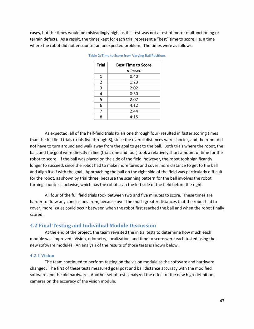
47
cases, but the times would be misleadingly high, as this test was not a test of motor malfunctioning or
terrain defects. As a result, the times kept for each trial represent a “best” time to score, i.e. a time
where the robot did not encounter an unexpected problem. The times were as follows:
Table 2: Time to Score from Varying Ball Positions
Trial Best Time to Score min:sec
1 0:40
2 1:23
3 2:02
4 0:30
5 2:07
6 4:12
7 2:44
8 4:15
As expected, all of the half-field trials (trials one through four) resulted in faster scoring times
than the full field trials (trials five through 8), since the overall distances were shorter, and the robot did
not have to turn around and walk away from the goal to get to the ball. Both trials where the robot, the
ball, and the goal were directly in line (trials one and four) took a relatively short amount of time for the
robot to score. If the ball was placed on the side of the field, however, the robot took significantly
longer to succeed, since the robot had to make more turns and cover more distance to get to the ball
and align itself with the goal. Approaching the ball on the right side of the field was particularly difficult
for the robot, as shown by trial three, because the scanning pattern for the ball involves the robot
turning counter-clockwise, which has the robot scan the left side of the field before the right.
All four of the full field trials took between two and five minutes to score. These times are
harder to draw any conclusions from, because over the much greater distances that the robot had to
cover, more issues could occur between when the robot first reached the ball and when the robot finally
scored.
4.2 Final Testing and Individual Module Discussion At the end of the project, the team revisited the initial tests to determine how much each
module was improved. Vision, odometry, localization, and time to score were each tested using the
new software modules. An analysis of the results of those tests is shown below.
4.2.1 Vision
The team continued to perform testing on the vision module as the software and hardware
changed. The first of these tests measured goal post and ball distance accuracy with the modified
software and the old hardware. Another set of tests analyzed the effect of the new high-definition
cameras on the accuracy of the vision module.

48
4.2.1: Final Post Distance Testing
The team performed the final testing of the vision module using the same method as that in the
initial testing, as described in the Vision section of the Methodology.
Figure 35: Comparisons of Distances from Posts at Various Positions After Software Changes
As can be observed from the graph above, the results from the distance measurements show
great accuracy. Every perceived post distance is close to its respective real post distance. The results
are much more accurate than those measured in the initial testing. This increase in accuracy is most
noticeable for farther distance measurements, where the error was particularly large in the initial test.

49
Figure 36: Comparisons of Distances from Posts at Various Positions after Hardware Changes
As opposed to increasing the accuracy of post distance measurements, the new hardware
actually caused a slight increase in the error. Furthermore, during the testing, some posts did not get
seen at all, specifically during trial 2, where the posts were the furthest away from the robot. Even with
this decrease in accuracy, the results are still dramatically more accurate than the results acquired
during the initial testing phase.

50
4.2.2: Final Ball Distance Testing:
The team applied the same methodology for the ball distance calculations.
Figure 37: Difference between Observed and Real Ball Distance after Software Changes
The error shown in the graph above is very similar to the error found in the initial test. This is
due to the fact that very little changes were implemented that affected the ball distance calculation
algorithms.

51
Figure 38: Difference between Observed and Real Ball Distance after Hardware Changes
This graph demonstrates the ball distance error using the new hardware, which provides a
higher resolution camera, as well as more processing power. This power allows for the processing of
larger images, which is particularly important for calculating the distances of small objects such as balls.
Figure 39: Comparison of Differences between Observed Ball Distances for all Tests

52
As the graph above demonstrates, the new hardware greatly decreased the error in calculating
the ball distance. The decrease in error is particularly noticeable at long distances, where the error with
the new hardware was only a third as high as that with the old one.
4.2.2 Odometry
After implementing a system to calibrate linear corrections for the robots’ odometry, the same
odometry tests were run again to determine the level of improvement. For this iteration of tests, only
three data points were gathered at each target distance. As the initial tests show, the distances that the
robot moves have little spread, so it was not necessary to collect six data points at each distance.
Figure 40: Expected Forward Distance vs. Error
The forward odometry data shows considerable improvement from the initial tests. The error
stays around 115 mm, where previously it averaged around 300 mm, peaking at 500 mm. The linear
correction significantly improved the robot’s forward odometry, reducing the error by 62%.
0 200 400 600 800 1000 1200 1400 16000
20
40
60
80
100
120
140
160
180
200Forward Odometry Error
Expected Distance (mm)
Err
or
(mm
)

53
Figure 41: Expected Left Distance vs. Error
Similar results can be seen for the left odometry. Initially, the error averaged around 200 mm,
peaking at 350 mm. With the linear odometry correction in place, the left error averaged around 125
mm, peaking at 275 mm. Left odometry error was reduced in this case by 38%.
Figure 42: Expected Turn Angle vs. Error
The turn odometry results are about the same as in the initial odometry tests. Both average
around 35 degrees. The data still loosely follows a linear trend, however, so with more calibration it is
possible that this error could be reduced.
0 100 200 300 400 500 600 700 800 900 10000
50
100
150
200
250
300Left Odometry Error
Expected Distance (mm)
Err
or
(mm
)
0 20 40 60 80 100 120 140 160 180 2000
10
20
30
40
50
60Turn Odometry Error
Expected Angle (degrees)
Err
or
(degre
es)

54
Overall, the linear odometry corrections were successful. Error was significantly reduced in
almost all cases. Furthermore, more time spent calibrating could lower the error even more. Improving
the correctness of the odometry can greatly improve the accuracy of the localization module, since
odometry is one of the two major inputs to the module.
4.2.3 Localization
Tests similar to the initial localization tests were carried out with the new localization module.
The results are shown below, organized by which filter the localization module was running. All final
localization tests were run after the 2012 rule switch, which changed the two goal colors to a single
color.
4.2.3.1 Particle Filter
The particle filter system was completed as designed, but several unforeseen issues caused
delays in its implementation and testing. Furthermore, hardware limitations prevented the traditionally
use of a large number of particle – particle filters usually use particles on the order of hundreds or
thousands, whereas our implementation used one hundred and twenty. Despite this, when provided
with accurate sensor data, the particle filter was able to successfully determine the robot’s location on
the field.
The particle filter implementation for this project was determined to be too inaccurate for
constant use during the Robocup competition. Though the filter operated as intended, sensor
inaccuracies and limitations in processor power and available memory made reaping the benefits the
particle filter method offers over the Kalman filter method extremely difficult. This determination was
made based off tests conducted on a full field setup in the lab.
The main hurdle to using the particle filter was the hardware available. A particle filter’s
performance is largely based on the number of particles which it can track. Initially, the onboard
memory could only support sixty particles, which was increased to one hundred twenty by redesigning
the data structure which holds the particle data. Further increases in the number of particles were
prevented due to the amount of time required to perform calculations on the entire set of particles,
which increased by an exponential degree as the number of particles was increased.
Another hurdle to the use of the particle filter was the variability and frequency of data
provided. As goal posts were the primary landmark used to determine position, when the vision system
did not detect a post, the particle filter was severely hampered in its ability to increase the accuracy of
the robot’s position. Additionally, it was extremely difficult to detect robots on the field in certain
lighting conditions, which eliminated the primary method for determining which end of the field is being
viewed for a large percentage of the localization routine iterations.
In addition to issues with the filter itself, there were issues with the ability to efficiently test
potential solutions to software issues. The methods used to download code to the platform prevent use
of traditional debuggers, and compiling and running tests on the platform is time consuming.
Additionally, running tests directly on the platform can provide misleading results, as there are a
multitude of other systems causing variability in the test environment, which is not desirable for an

55
initial test environment. These problems were addressed by creating a test setup with a simulated robot
and program framework, allowing isolation and debugging of specific particle filter operations.
Aside from this, the filter performed well, especially taking into account the limitations placed
upon it. The filter could accurately determine the robot’s position given accurate sensor data in a short
amount of time. It correctly eliminated and replaced low probability particles in a way which increased
the overall accuracy of the predicted position over time. Further, the filter accounted for odometry data
and was designed in a way to be extensible should other landmarks be made available from vision to
localize off of.
There are several ways to improve the performance of the particle filter system from its current
state. The highest positive impact on the filter’s performance would be gained by finding a way to
significantly increase the number of particles used by the filter. This could be done by finding ways to
perform operations on multiple array indices at once (technology which is already used in GPUs), and
finding ways to reduce the number of times the array of particles is iterated over each localization
routine iteration.
Another way to improve the performance of the filter would be to pre-process the provided
data more extensively. One option for this is to check the variability of consecutive post distance and
heading readings, and to evaluate how accurate the odometry readings are based on the particle filter’s
position data, fusing those values using a weighting system.
Additionally, the algorithm to determine the boundaries within which new particles are
generated could be improved. Currently, the algorithm evaluates the density of particles within an area
and picks the highest value. Instead, each particle could be surrounded by a box of a standard size.
Overlapping boxes could be combined, until all remaining boxes are completely separate. The two boxes
whose contained particles had the highest average probability would be selected for use, and new
particles would be generated within them. This algorithm is potentially more efficient and more
accurate in determining particle regions, which would lead to better performance and better run times.
4.2.3.2 Kalman Filter
Results of testing the Kalman Filter were generally favorable compared to the old localization
module. As with the previous tests, the robot ran its behavior code under game conditions while
localization data was gathered. Below is a comparison of the robot’s estimated trajectory and the
robot’s actual trajectory.

56
Figure 43: Kalman Filter Trajectories and Error
The trajectories alone may initially seem to be quite erroneous, but when the error is taken into
account it shows that the position is not as bad as it looks. The jump to the right of the estimated
trajectory is only a single jump in error, and the robot actually managed to correct this error as the test
continued. Looking at the graphs of error percentages, it remains low throughout most of the test for x,
y, and theta. The error propagated a bit as the test went on, but this is to be expected with a Kalman
filter, and as the robot saw more goals, the error was corrected.
After the rule change made both team’s goals the same color, another test was devised for the
localization module. The robot was placed on the field with a goalie in each goal, and allowed to kick
the ball around until it scored in one of the goals. After performing this test multiple times, the robot
consistently scored in the enemy goal. There were situations where the robot would kick the ball
towards its own goal, but once it got close, the localization module corrected its position and it returned
to aiming at the enemy goal.
Between these two tests it is clear that the Kalman filter localization is a significant
improvement on the original localization module. Error was lower overall, and the robot was able to
recover from error given enough time. More importantly, the new localization was sufficient to prevent
the robot from scoring on its own goal, whereas the original localization was not consistent enough to
handle the same color goal case.
The biggest issue with the Kalman filter is that it does not handle the case of penalization when
a robot is “kidnapped.” Since it requires an accurate previous position to run effectively, being picked
up and moved messes up the calculations significantly. The robot can eventually re-localize, but it takes
some time due to the smoothing effects of the Kalman filter algorithm. This could be improved
somewhat by using communication with other robots to determine which side of the field the robot is
entering after penalization. Further improvements to the general algorithm could be made by localizing
-2000 -1000 0 1000 2000-3000
-2000
-1000
0
1000
2000
3000
Field Width (mm)
Fie
ld H
eig
ht
(mm
)
Localization Trajectory
Estimated Trajectory
Actual Trajectory
0 10 20 30 40 50 60 70 800
10
20
30
40
50
60
70
80
90
100
Time (s)
Err
or
(%)
Localization Error
x Error
y Error
theta Error

57
based off of the white field lines on the soccer field instead of using only the goal posts and the field
edges.
4.2.3.3 Complete Localization System
The original plan for the localization system was to switch between the Kalman and particle
filters. However, this proved to be untenable, as the particle filter was unable to perform to the required
level on the hardware available. The particle filter ran slowly due to the number of particles it has to
maintain, and its accuracy and speed of improvement were limited due to the issues with the number of
particles that could be tracked at one time. The final setup of the system was to use the Kalman filter
with a relatively accurate estimated initial position. This took some burden off the processors, and was
accurate enough for the purposes of the project.
The problems of the Kalman filter, specifically the inability to localize quickly after penalization,
did become more apparent once the particle filter was dropped. The particle filter was specifically
implemented to handle this case, so as only the Kalman filter was used, the localization system as a
whole was not optimal. The biggest improvement to the localization module as a whole would be
realizing the successful implementation of particle and Kalman filter switching.
4.2.4 Time to Score
Repeating the time to score tests with the new code proved difficult. With the change in the
game rules resulting in two goals of the same color, comparisons to the old time to score tests do not
necessarily make sense. Furthermore, due to bugs introduced by the new robot heads, the results were
highly inconsistent.
Running the half-field time to score tests produced equivalent times for the robot to score
provided that the ball was directly in line with the goal. However, whenever the ball was placed on the
sides of the field, unsolved vision bugs caused by the new heads prevented the robot from scoring in a
reasonable time frame.
Theoretically, the times should have been improved, and the original bias for scoring on the left
side of the field faster than the right should have been eliminated. This is because the new behavior
code, in conjunction with the new localization code, was specifically written to allow the robot to turn in
the optimal direction at any point on the field. Subjective evaluation of a robot’s turn direction
decisions showed that the robot turned in the correct direction most of the time, from many different
locations on the field. Due to the bugs with the new heads, a more objective evaluation of
improvements on the robot’s time to score was unable to be conducted.
4.3 Discussion of the System Performance as a Whole The entire system ran effectively enough to keep the WPI team competitive with the other US
teams. Out of the eight teams that registered for the SPL US Open competition, two teams dropped out
to continue developing their code for next year’s competition. Of the remaining six teams, WPI placed
in fourth.

58
Improvements to each individual module worked well in conjunction with the other modules.
The distance improvements to the vision module and the linear corrections to the odometry data
allowed the localization module to determine a more accurate position. The improved localization
module, with the addition of goalie detection, allowed the behavior module to make more informed
decisions. These localization-based decisions allowed the robot to improve the overall soccer strategies
used in a game situation, significantly improving the team’s performance.
5 Conclusion and Recommendations This project successfully met almost all of its initial goals. The vision system was significantly
improved, providing more accurate range and heading data to the goal posts, and eliminating a large
number of false positives. This made the information gathered in the vision module significantly more
useful to the localization module.
The localization system was able to determine the robot’s position based on sighted goal posts.
The particle filter was not optimized enough to be practically used, however it was still successful in
determining the robot’s position when tested. Its speed and efficiency could be improved by finding
ways to increase the number of particles which can be tracked by the filter, and optimizing the filter
further for a low memory and processor speed environment. Additional improvements to the
localization system as a whole could include the use of field lines for localization, as well as
implementing sanity checks by using the relative position of the ball from the goalie compared to the
perceived ball position of the player running the algorithm.
Behaviors were improved from the previous year’s competition code. The robot could more
effectively use localization information in deciding what actions to take, such as which direction would
be faster to turn, and when the robot should clear the ball in a general forward direction rather than aim
directly at the goal. Role switching with a support role was not fully tested, and future work in role
switching is recommended, as this is often the difference between the best teams and the middle-of-
the-pack teams.
The motion module was more or less untouched for this project, aside from implementing a
linear correction for the robot’s odometry data. The code base could be significantly improved by
developing a better humanoid walk engine, as well as a library of kicks for different situations. This is a
huge endeavor, however, and was outside of the scope of this project.
Despite plans at the beginning of the year to develop a replacement for rUNSWift’s visualization
tool OffNao, the web visualization tool cannot replace OffNao. The visualization tool was a step in the
right direction in terms of a creating a new tool that will eventually act as cross-platform tool for
developing and testing the robots. Future work on the visualization tool would include allowing users to
calibrate the robots directly from the web. Additionally, more work could be done to allow better
gathering and logging of data from the robot. Particularly, it would be useful to provide some control to
the user via the interface for moving the robot’s head during calibration.

59
Overall, the project was successful. With the current state of the code, the robots could
effectively play a game of soccer. The WPI team came in fourth place out of the eight teams initially
registered for the RoboCup US Open competition. With a bit more work, the WPI Warrior’s standing
among the US Standard Platform League teams could certainly improve.

60
References
Aldebaran Robotics. (2012). Hardware platform - corporate - aldebaran robotics | key features. 2012, from http://www.aldebaran-robotics.com/en/Discover-NAO/Key-Features/hardware-platform.html
Barrett, S., Genter, K., Hausknecht, M., Hester, T., Khandelwal, P., Lee, J., et al. (2010). Austin villa 2010 standard platform team report No. 1). Austin, Texas.
Brindza, J., Cai, L., Thomas, A., Boczar, R., Caliskan, A., Lee, A., et al. (2010). UPennalizers RoboCup standard platform league team report 2010 No. 1). Philadelphia, Pennsylvania: University of Pennsylvania.
Czarnetzki, S., Kerner, S., Urbann, O., Hofmann, M., Stumm, S., & Shwarz, I. (2010). Nao devils dortmund team report 2010 No. 1). Dortmund: Technische Universitat Dortmund.
Freeston, L. (2002). Applications of the Kalman filter algorithm to robot localisation and world modeling. University of Newcastle, NSW, Australia: Retrieved from http://www8.cs.umu.se/research/ifor/dl/LOCALIZATION-NAVIGATION/Applications%20of%20the%20Kalman%20Filter%20slgorithm%20to%20robot%20localization%20and.pdf
Ivanjko, E., Kitanov, A., & Petrovic, I. (2010). Model based Kalman filter mobile robot self-localization. InTech, , 59-90. Retrieved from http://www.intechopen.com/source/pdfs/10566/InTech-Model_based_Kalman_filter_mobile_robot_self_localization.pdf
Leonard, J. J., & Durrant-Whyte, H. F. (1991). Mobile robot localization by tracking geometric beacons. Robotics and Automation, IEEE Transactions on, 7(3), 376-382. Retrieved from http://ieeexplore.ieee.org/xpls/abs_all.jsp?arnumber=88147
Martinez-Gomez, J., Jimenez-Picazo, A., & Garcia-Varea, I. (2009). A particle-filter-based self-localization method using invariant features as visual information. Spain: University of Castilla-La Mancha. Retrieved from A particle-filter-based self-localization method using invariant features as visual information
Negenborn, R. (2003). Robot localization and Kalman filters: On finding your position in a noisy world. (Master of Science, Utrecht University). Retrieved from http://www.negenborn.net/kal_loc/thesis.pdf
Peli, T. (1982). A study of edge detection algorithms. Computer Graphics and Image Processing, 20, 1. Retrieved from http://www.sipl.technion.ac.il/new/Staff/Academic/Malah/Publications/Peli_Edge_Detection_1982.pdf
Ratter, A., Hengst, B., Hall, B., White, B., Vance, B., Sammut, C., et al. (2010). rUNSWift team report 2010 robocup standard platform league No. 1). Sydney, Australia: University of New South Wales.

61
Rekleitis, I. (2004). A particle filter tutorial for mobile robot localization No. TR-CIM-04-02) Centre for Intelligent Machine, McGill University.
RoboCup Technical Committee. (2012). RoboCup standard platform league (nao) rule draft. The Robocup Federation.
The Robocup Federation. (2012). RoboCup. 2012, from http://www.robocup.org/

62
Appendix A: RoboCup Standard Platform League Qualification Report

63
WPI Warriors
Team Description, Standard Platform League 2012
Irena Cich, Frederik Clinckemaillie, Runzi Gao, David Kent, Benjamin Leone, Miaobo Li, Derek
MacNeil-Blackmer, William Mulligan, Ryan O’Meara, Quinten Palmer, Alexander Ryan, and
Sonia Chernova
Worcester Polytechnic Institute
100 Institute Rd.
Worcester, MA 01609 USA
Abstract. This paper outlines the organization and architecture of the
WPI Warrior’s 2012 robotic soccer team developed at Worcester
Polytechnic Institute. The team is made up of undergraduates and
graduates ranging from freshman level to first year graduates. The team
software architecture is based on the rUNSWift 2010 open source code
release from the University of New South Wales. This paper reports on
the current state of the software development and documents the
modifications made to the rUNSWift software architecture.
1 Introduction and Statement of Commitment The WPI Warriors first competed in the RoboCup Standard Platform League last year.
Upon qualification, the team plans to compete in the RoboCup Standard Platform League 2012
competition. The team consists of undergraduate and first-year graduate students, led by
Professor Sonia Chernova. This document outlines our current software, as well as our planned
research for the upcoming competition.
2 Software Architecture Overview Our software architecture is based off of the software architecture of the rUNSWift team
[2]. We are replacing and modifying modules as we develop. We have developed our own
localization and behavior modules. We have modified the vision module and intend to modify
the motion engine. We intend to add more to the world model as we add new features, but the
main focus of our work this year has been to replace as much of rUNSWift’s code with our own
code as possible. We have modified rUNSWift's tools for syncing code and are using their
OffNao GUI only for calibration, and we have developed our own tools for visualization and
compilation. Below is a representation of our software architecture.

64
Figure 44. Software Architecture Overview
3 Vision The vision module has been modified to increase performance in detecting and analyzing
objects. The low level calculations and calibration have remained unmodified, and are based on
the rUNSWift architecture [2]. The main priorities in changing the vision module were in the
goal detection and analysis. The localization module relies heavily on goal posts, and as such we
have worked on optimizing the correct identification of goal posts (i.e. reducing false positives
and negatives) and increasing the accuracy of goal post analysis (i.e. correct distance and
heading, especially at greater distances).
We plan to add more to the vision module in the future. Our next priority is to implement
line detection. This addition would give another input to the localization module. Currently the
localization module is heavily reliant on goal post information determined by the vision module,
but there are many cases in a game situation where a robot will not see any goal posts. Adding
accurate line detection would allow the robot to localize more effectively during these situations.

65
4 Localization The localization module has been significantly improved upon from the localization
module used by the team at the RoboCup 2011 Standard Platform League competition.
Previously, the robot performed basic localization based on odometry information and goal post
readings. During fall and winter of 2011, the team rewrote the localization module to utilize a
particle filter to determine a robot’s initial position on the field. Once this initial position is
determined, the localization module switches to use Kalman filtering to smooth any positional
changes. If the robot loses confidence in its position, the localization module will switch back to
the more computationally intensive particle filter to re-establish an initial position for the
Kalman filter.
Currently, odometry and goal posts are the only inputs to the localization module. In the
coming months, we plan to add rudimentary field line localization to the particle and Kalman
filters using the center circle and field line corners.
5 Motion The majority of our motion code utilizes the rUNSWift motion architecture [2]. Our
code currently uses a walk generated from rUNSWift’s code and a static forward kick that can be
mirrored onto either the left or right foot. We plan to improve both the walk engine and our
library of kicks before the upcoming competition. Projected improvements to the walk engine
include optimizing the motion for use on carpet to prevent overheating of the robot’s hip and
knee joints, and improving the overall stability of the robot. The team is also developing static
sideways and backwards kicks, as well as short-range kicks with low execution times. Goalie
blocking motions are also under development.
Another improvement we plan to make for the motion module deals with the current
odometry code. The current software uses the same odometry calculation for each robot, despite
the fact that all four of our robots have slight differences in their physical motion. To counteract
this problem, we plan to implement an odometry configuration file that will correct odometry
readings. This would allow each robot to have individual odometry calibration before each
game.
6 Behavior The behavior module is the highest-level module in our software architecture. To allow
for quick editing, we implement behaviors in Python (rather than the C++ used for all of the
lower-level modules). Behaviors are broken down into individual skills, such as scanning with
the head, tracking a ball, or aligning on a goal, and behaviors, which implement one or more
skills to accomplish a task, such as walking to the ball.

66
The module uses a finite state machine to determine which behaviors to use in what
order. Depending on certain conditions, when a behavior is determined to be finished, it will
push itself onto a stack and activate the next appropriate behavior. Each robot role (e.g. striker,
goalie, supporter, defender) is defined by a different branching behavior stack. An example
stack for a Striker is shown below, where a down arrow represents pushing the current state onto
the stack and activating the state below it, and an up arrow represents popping the above state off
of the stack.
Figure 45. Striker Behavior Stack Example
Based on certain conditions, the currently used behavior stack can be switched to the
stack of another robot role. For example, if two strikers detect the ball at the same time, the
striker that is farther from the ball will switch to the supporter role, leaving the closer striker to
get to the ball.

67
7 World Model The World Model is where all of the shared information is stored. Vision, Localization,
Motion, Behaviors, Game Controller, Receiver, and Trasmitter are the main modules that write
to and read from the world model. This module is used to allow each of the modules to
communicate with each other, and to maintain an overall representation of the state of the game.
8 Acknowledgements Special thanks to the University of New South Wales rUNSWift team for making their
code available to the research community. We also thank Worcester Polytechnic Institute for
financial support for this project.
References 1. Sonia Chernova, Frederik Clinckemaillie, Christopher Conley, Runzi Gao, David Kent, Benjamin Leone, William
Mulligan, Khan-Nhan Nguyen, Quinten Palmer. WPI Warriors: Team Description, Standard Platform
League 2011.
2. Adrian Ratter, Bernhard Hengst, Brad Hall, Brock White, Benjamin Vance, Claude Sammut, David Claridge,
Hung Nguyen, Jayen Ashar, Maurice Pagnucco, Stuart Robinson, Yanjin Zhu. rUNSWift Team Report:
Robocup Standard Platform League 2010.


![[ , ] Autonomous Human Robot Interactive Skills](https://img.pdfslide.us/doc/110x75/577cc35f1a28aba71195d883/-autonomous-human-robot-interactive-skills.jpg)