Project final: epitope classification using support vector machines

Bornika Ghosh and Andrew Parker

June 2, 2009

1 Introduction

The human body immune response to a vaccine or protein therapeutic largely determines the utility of thatdrug. Promising medicines which cause an immune reaction are unfortunately not usually viable. An im-mune function begins when so called antigen presenting cells (APC) ingest and digest exocellular biologicalmolecules and display short parts of the cleaved antigen, an epitope, on the cell surface by binding the epi-tope to a Class II major histocompatibillity complex (MHC). The binding between an MHC protein and anepitope is the first stage, the detection step, in the bodies adaptive immune response to an antigen. [3] Ifprotein engineers could predict which epitopes bind to MHC, then they could design therapeutic proteinsthat are less likely to elicit an immune response from patients, which as mentioned, typically renders amedicine useless. The accumulation of large quantities of data about MHC protein structure and functionhas allowed the application of bioinfomatics and machine learning techniques to make realistic models,and hence predictions, of which epitopes bind and do not bind to MHC. Indeed many reviews describe theproblem motivation and current work in the field. [5, 14]

We seek to classify epitopes as binders or non-binders to specific MHC Class II alleles. Several curateddatabases contain thousands of epitopes characterized through biological assays. [6, 8] A typical entry ina database contains the epitope primary structure, the MHC Class II allele to which the epitope binds andthe binding affinity. The binding affinity can be expressed as a discrete class, for example as none, mild,moderate, or high; or it can be expressed as a positive real number, usually as the IC50 value.

Due to the scientific interest and practical importance of these predictions a literature exists to assessthe accuracy of prediction tools. Not only can we compare our results to published results, but we canalso directly use publicly available data sets and webservers from this literature to test and compare ourimplementation. [4, 9] One popular tool in particular to compare against is the ProPred webserver. [11]ProPred uses ”virtual” matrices which are calculated with mostly bioinformatics tools such as sequence andstructure alignment of different MHC Class II alleles. In this fashion biological data available from one allelecan be applied towards modeling the other. It is interesting to compare and contrast purely machine learningtools, such as SMM-align [7] or our SVM implementation, with the ProPred bioinformatics approach.

2 Methods

2.1 Learning Feature Vectors and Kernels

The variable length epitope sequences are first converted into fixed length feature vectors. The epitopesare short sequence of amino acids, and a feature vector has to be constructed to represent the structural andphysico-chemical properties of the peptides. Each of the feature vectors is 21 elements long. [2] We divided

1

!"#$%&'()*+,-./012(.3'&%()45678!12(/9:%3;<3=>?()@ABCDEF1(

-39(.";$>:"(G(+6+6B6++66+6D6++6(

!(H(IJ(

!(H(KLIM!N(LOM!N(LPM!Q(

LI(H(JK+QN(LO(H(RK6QN(LP(H(OKDNBQ(

@(H(KSTUIIRN(STUJSVNSTIIJVQ(

"(H(K-*I*OM!WIN(-*O*PM!WIN((-*I*PM!WIQ(

-*I*O(H(X(+!6(Y(6!+((

-*O*P(H(O(6!B(Y(B!62(O(6!D(Y(D!6(

-*I*P(H(S(+!D(Y(D!+(

-(H(KSTZVOZNSTOZNSTSQ(

#(H(K7IN(7ON(7PQ(

#$(H(K.>SM!N(.>OZM!N(.>ZSM!N(.>JZM!N(.>ISSM!Q(

!"!"#"!!""!"$"!!"%

&'%(%)'*'+,%-*'+,%.*'+,%''*'+,%'/*'+0%

7(H(KSTSZRRNSTIJVZNSTUJSVNSTVUJIN(STXUIONSTIIJVNSTOPZPNSTZOXUNSTJSZX((

((((((((((((NITSSSSNSTOXUINSTOXUINSTOXUI(NSTJVUJNSTJVUJQ(

Figure 1: Example derivation of a feature vector.

the 20 amino acids into three groups based upon their hydrophobicity, rather than treating each of the 20amino acids as a separate group. This is done because many amino acids have same hydrophopic properties,and can be treated as a group, rather than redundantly treating each of them as a separate group. We thendefined 3 descriptors, composition (C), transition (T) and distribution (D), to describe the global compositionof the epitopes. The descriptor C was computed as a vector of 3 real numbers, each corresponding to thefraction of amino acids for each of the above 3 groups, found in the epitope. So C1 gave the fraction of aminoacids from group one, C2 from group 2 and C3 from group 3 in the epitope. The descriptor T characterizesthe fraction of frequency with which amino acids from a group are followed and preceded by amino acidsfrom a different group. T1 gives the fraction of transitions from class 1 to class 2, T2 gives the fraction oftransitions from class 1 to class 3, and T3 gives the fraction of transitions from class 2 to class 3. The thirddescriptor D, is the chain length up to which, the first, 25%, 50%, 75% and 100% of amino acid of eachclass are found in the peptide sequence. We have D1, D2 and D3 for the 3 groups mentioned above and eachof these, have 5 elements for first, 25%, 50%, 75% and 100%. Hence the feature vector consists of 3 + 3 +(3*5) features, making it a 21 element long vector Fig. 1.

We create the feature vectors for all the epitopes. These feature vectors form the input to the SVMlearning algorithms. We tried to learn first a linear SVM model for the feature vectors. We used MATLABfunction quadprog for it for the dual problem. The MATLAB function quadprog did not converge. Wethen tried the C-SVC program with the RBF kernel of the LIBSVM software package [1]. Next we learntthe SVM parameters using Manik Varma’s algorithm GMKL [13], which is a generalized multiple kernel

2

learning algorithm. Multiple kernel learning algorithms learn a linear combination of base kernels from thetraining data. Manik Varma et al. extended the idea of combining kernels to a non-linear combination ofbase kernels. The algorithm works in two stages, in the outer loop, the kernel is learnt by optimizing over theweights of individual kernels, and in the inner loop the SVM parameters are learnt using the present value ofthe kernel. This is continued till convergence of the SVM parameters. The step size used in the outer loopis chosen based on the Armijo rule to guarantee convergence and then a projection of the weights vector ismade. We used 3 different kernel options within GMKL, sum of RBF of individual kernels, product of RBFof individual kernels and product of exponential kernel of pre-computed distance matrices.

2.2 Datasets

We downloaded the binder and non-binder epitope data from MHCBN database for three different alleles,HLA-DRB1*0301, HLA-DRB1*0701 and HLA-DRB1*1101 (allele 3, 7 and 11 respectively). These datasets have unique lists of peptides for binders and non-binders (UPDS). The number of non-binders (200+)is generally less than the number of binders (500+), hence we could not do cross-validation for training theSVM parameters. We chose a set of 100 binders and 100 non-binders randomly to construct the trainingdata set. The remaining data from the set of unique peptides was used as test data. We carried out theexperiments on a range of subsets of the training data set. The sub sets were chosen by incrementing thenumber of examples on which to train the SVM. We started with 20 epitopes, 10 of each class, and wenton to increase the number of training examples to 200, 100 of each class. We learn separate SVMs foreach different allele. After the SVM parameters were learned, we tested it on the respective test data set(mentioned above). We also tested the learnt SVMs for each allele on similarity reduced test data sets. Thesewere downloaded from (give the site name). These data sets have been created so that, the epitopes in thesedatasets are only some percentage similar to each other. The first reduced similarity data set is SRDS1; thisdata set is constructed from the UPDS data set such that none of the epitopes in SRDS1 have a common 9residue long subsequence. The second reduced similarity data set is SRDS2; this data set is constructed fromSRDS1 by throwing away epitopes that are 80% or more similar to any of the other epitopes. The third dataset SRDS3 is constructed from UPDS by applying similarity reduction techniques introduced by Raghava[9]. We used the data for each of the above-mentioned alleles from the 3 similarity reduced datasets to carryout further tests with the learnt SVMs.

3 Results

3.1 Support Vector Machines

Fig. 2 and Fig. 3 show the plots of error rate vs. the training sample size for different datasets for Allele3. Fig. 4 and Fig. 5 show the plots of error rate vs. the training sample size for different datasets for Allele7. Fig. 6 and Fig. 7 show the plots of error rate vs. the training sample size for different datasets for Allele11. LIBSVM and Manik Varmas model with the sum of RBF kernels of individual features have a problemof being underfit models. The former uses a RBF kernel over all features and the latter uses sum of RBFkernels of individual features. Manik Varmas model with the sum of RBF kernels of individual featuresperforms slightly better than LIBSVM, but both of them do not increase the dimension. The kernels used ineither of these methods are not complex enough to separate the binding epitopes from the non-binding ones.Hence increasing the size of the training set does not help to reduce error-rate for prediction of binders fromnon-binders. These two methods across all 3 alleles have shown a rise in the training set error rate. The other2 methods, namely Maniks code with the product of RBF kernels of individual features and Maniks code

3

with the product of kernels of pre-computed distance matrices of the objects are better fitting models for thepurpose of classification of epitopes into binders and non-binders. The higher dimensional kernels (tensorproduct) can actually differentiate the data better. Similarity reduction in data sets improves the performanceof all the methods. For Allele 3 and Allele 7 the error rate for non-binder prediction is higher than binderprediction, but for Allele 11 its vice-versa across the methods using GMKL techniques.

3.2 SVM compared with ProPred and SMM-align

We compared the results obtained by using LIBSVM and Manik Varmas algorithm with various kerneloptions with the prediction results of the same test data sets obtained from ProPred and SMM-Align. Fig. 8

ProPred is a webserver based on the method of Sturniolo. [12] Sturniolo’s group sought to characterizeeach of the 9 binding positions independent of each other on over 50 different MHC Class II alleles. Es-sentially they measured the binding affinity of each of the 20 amino acids to each of the 9 binding positionson a limited number of alleles with known structure. Call these alleles characterized and the other allelesuncharacterized. They performed sequence and structural alignment between characterized and uncharac-terized alleles for each of the 9 binding positions. The uncharacterized allele binding positions were said tohave the same properties as the characterized allele binding positions with which they best aligned. Bind-ing positions were aligned independently so an uncharacterized allele could take the properties of bindingposition 1 from a certain allele and the properties of binding position 2 from a different allele and so on. Inthis fashion over 50 different 20 by 9 ”virtual” position specific scoring matrices were derived. The bindingaffinity of a 9mer peptide to an allele is equal to the sum of the scores at each position from the allele virtualmatrix. ProPred considers a peptide a binder to an allele if the binding affinity between peptide and allele isgreater than a threshold. The weakest threshold is set equal to the average score of the top 10% of 9mers.

SMM-align is a machine learning method implemented on the netMHCII webserver. [10] Nielsen andhis group also learn 20 by 9 position specific scoring matrices for each allele; however, they learn scores witha regularized least mean squares method directly from measured IC50 binding affinity values and peptideprimary structure now available in large databases. Their matrices predict the IC50 binding affinity value ofinput peptides. Generally, a binding value less than 50 is considered a strong binder, a binding value of lessthat 500 is considered a fair binder, and a binding value of less than 5000 is considered a weak binder. Noknown validated epitopes have a measured value greater than 5000.

Both ProPred and SMM-align implement an important expert rule, namely, only 7 hydrophobic aminoacids (F, I, L, M, W, V and Y) may occupy binding position number 1 in a bound MHC Class II peptide.Had we more time, we would have implemented this rule for SVM.

Each of the different methods have similar misclassification rates for binders and non-binders of the 3alleles across the 3 similarity reduced datasets, i.e. for every method, the misclassification rates of bindersand non-binders are almost same for the different similarity reduced data sets of the 3 alleles. The error ratesare mostly lower for the similarity reduced dataset than for the unique peptide data sets (UPDS) for bothbinders and non-binders of all alleles, across all methods. SMM-Align does the worst in predicting bindersacross all datasets for the 3 alleles and best when predicting non-binders for Allele 3 and Allele 11. ProPreddoes better on binder prediction than SMM-Align but performs worse than the other methods. LIBSVMand Manik Varmas code with the sum of RBF kernels of individual features perform similarly across alldatasets, though the latter is slightly better than the former. Maniks code with the product of RBF kernelsof individual features and Maniks code with the product of kernels of pre-computed distance matrices of theobjects give the exact same errors for binder and non-binder prediction across all data sets. Also these twomethods have the best overall performance because of the higher dimensional kernels that they use.

4

Figure 2: allele 3

5

Figure 3: allele 3

6

Figure 4: allele 7

7

Figure 5: allele 7

8

Figure 6: allele 11

9

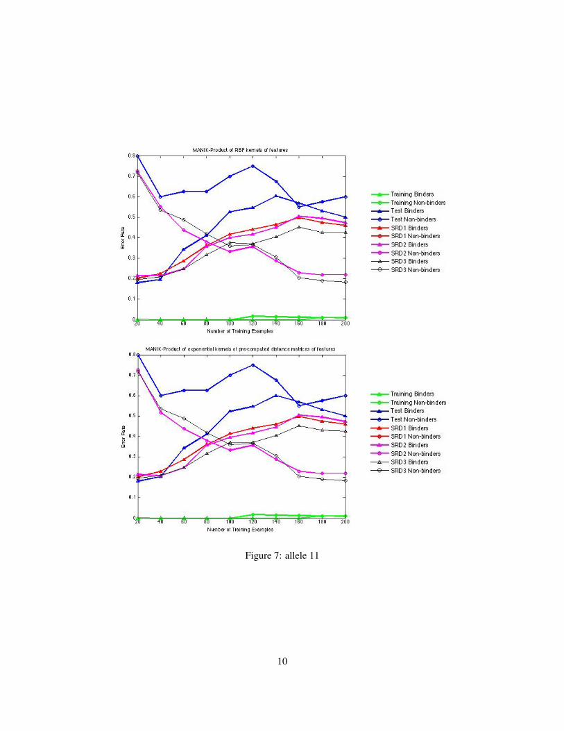
Figure 7: allele 11

10

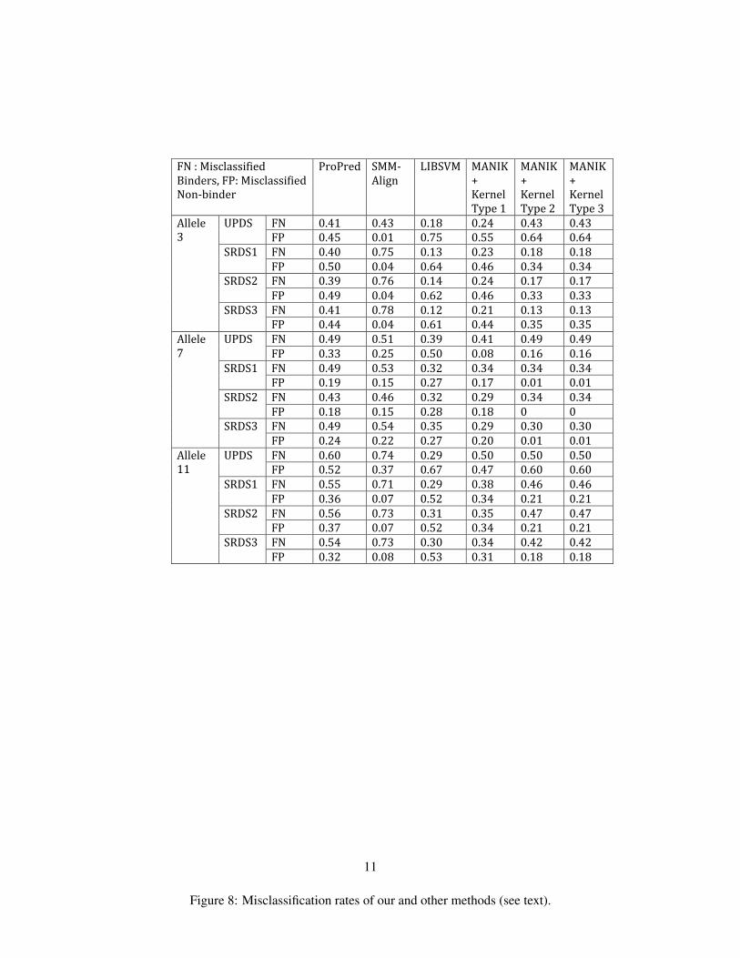
FN:MisclassifiedBinders,FP:MisclassifiedNon‐binder

ProPred SMM‐Align

LIBSVM MANIK+KernelType1

MANIK+KernelType2

MANIK+KernelType3

FN 0.41 0.43 0.18 0.24 0.43 0.43UPDSFP 0.45 0.01 0.75 0.55 0.64 0.64FN 0.40 0.75 0.13 0.23 0.18 0.18SRDS1FP 0.50 0.04 0.64 0.46 0.34 0.34FN 0.39 0.76 0.14 0.24 0.17 0.17SRDS2FP 0.49 0.04 0.62 0.46 0.33 0.33FN 0.41 0.78 0.12 0.21 0.13 0.13

Allele3

SRDS3FP 0.44 0.04 0.61 0.44 0.35 0.35FN 0.49 0.51 0.39 0.41 0.49 0.49UPDSFP 0.33 0.25 0.50 0.08 0.16 0.16FN 0.49 0.53 0.32 0.34 0.34 0.34SRDS1FP 0.19 0.15 0.27 0.17 0.01 0.01FN 0.43 0.46 0.32 0.29 0.34 0.34SRDS2FP 0.18 0.15 0.28 0.18 0 0FN 0.49 0.54 0.35 0.29 0.30 0.30

Allele7

SRDS3FP 0.24 0.22 0.27 0.20 0.01 0.01FN 0.60 0.74 0.29 0.50 0.50 0.50UPDSFP 0.52 0.37 0.67 0.47 0.60 0.60FN 0.55 0.71 0.29 0.38 0.46 0.46SRDS1FP 0.36 0.07 0.52 0.34 0.21 0.21FN 0.56 0.73 0.31 0.35 0.47 0.47SRDS2FP 0.37 0.07 0.52 0.34 0.21 0.21FN 0.54 0.73 0.30 0.34 0.42 0.42

Allele11

SRDS3FP 0.32 0.08 0.53 0.31 0.18 0.18

Figure 8: Misclassification rates of our and other methods (see text).

11

4 Conclusion

Fewer numbers of non-binders in the data sets lead to less representation of non-binders and may be thecause of higher misclassification rates in predicting non-binders. Increasing the number of features couldhave further reduced the error rates. Had we more time, we could have extended the feature space to includemore physico-chemical features like solvent accessibility, normalized Vander-Waals volume, surface tensionand secondary structures to name a few. Generalized Multiple Kernel Learning (GMKL) algorithm seeksto improve classification, using SVM by learning and using non-linear combinations of kernels. The factthat Manik s code along with products (tensor) of kernels of individual features and pre-computed distancematrices produces better classification results than using a single kernel (LIBSVM) or a linear combinationof kernels (Maniks code with sum of RBF kernels) shows that GMKL is indeed a better approach than MKL.

References

[1] Chih-Chung Chang and Chih-Jen Lin. LIBSVM: a library for support vector machines, 2001. Softwareavailable at http://www.csie.ntu.edu.tw/˜cjlin/libsvm.

[2] J. Cui, L. Y. Han, H. H. Lin, H. L. Zhang, Z. Q. Tang, C.J. Zheng, Z.W. Cao, and Y.Z. Chen. Predictionof mhc binding peptides of flexible lengths from sequence-derived structural and physicochemicalproperties. Mol Immunol., 44(5):866–77, 2007.

[3] A. L. DeFranco, R. M. Locksley, and M. Robertson. Immunity. Oxford University Press, 2007.

[4] Y. EL-Manzalawy, D. Dobbs, and H. Vasant. On evaluating mhc-ii binding peptide prediction methods.PLoS ONE, 3:e3268, 2008.

[5] A. S. De Groot and L. Moise. Prediction of immunogenicity for therapeutic proteins: State of the art.Current Opinion in Drug Discovery and Development, 10(3):332–340, 2007.

[6] S. Lata, M. Bhasin, and G. P. S. Raghava. MHCBN 4.0: A database of MHC/TAP binding peptidesand T-cell epitopes. BMC Research Notes (In press), 1:1, 2009.

[7] M. Nielsen, C. Lundegaard, and O. Lund. Prediction of mhc class ii binding affinity using smm-align,a novel stabilization matrix alignment method. BMC Bioinformatics, 8:238, 2007.

[8] B. Peters, J. Sidney, P. Bourne, H. H. Bui, S. Buus, G. Doh, W. Fleri, M. Kronenberg, R. Kubo,O. Lund, and et al. The immune epitope database and analysis resource: from vision to blueprint.PLoS Biol, 3:e91, 2005.

[9] G. Raghava. MHCBench: Evaluation of MHC binding prediction algorithms. available athttp://www.imtech.res.in/raghava/mhcbench/.

[10] CBS Prediction Servers. NetMHCII. http://www.cbs.dtu.dk/services/NetMHCII/.

[11] H. Singh and G.P.S. Raghava. ProPred: prediction of HLA-DR binding sites. Bioinformatics, 17:1236–1237, 2001.

[12] Sturniolo. T., E. Bono, J. Ding, L. Raddrizzani, O. Tuereci, U. Sahin, M. Braxenthaler, F. Gallazzi,M.P. Protti, F. Sinigaglia, and J. Hammer. Generation of tissue-specific and promiscuous hla ligand

12

databases using dna microarrays and virtual hla class ii matrices. Nat. Biotechnol., 17(6):555–561,1999.

[13] M. Varma and B. R. Babu. More generality in efficient multiple kernel learning. to appear Proceedingsof the 26th International Conference on Machine Learning, 2009.

[14] S. Vivona, J. L. Gardy, S. Ramachandran, F. S. L. Brinkman, G. P. S. Raghava, D. R. Flower, andF. Filippini. Computer-aided biotechnology: from immuno-informatics to reverse vaccinology. Trendsin Biotechnology, 26(4):190–200, 2007.

13