Embed Size (px)
Citation preview
Harpur Hill, Buxton Derbyshire, SK17 9JN T: +44 (0)1298 218000 F: +44 (0)1298 218590 W: www.hsl.gov.uk
Investigation of the dynamic behaviour of aluminium welds in rail vehicle applications
HSL/2006/95
Dr William Geary Project Leader:
Author(s): Mr Chris J Atkin BEng (hons)
Dr Pete Apps BEng
Science Group: Engineering Control Group
© Crown copyright (2006)
CONTENTS
1 INTRODUCTION......................................................................................... 11.1 Background ............................................................................................. 11.2 Sample preparation ................................................................................. 2
2 TEST PROGRAMME.................................................................................. 32.1 Instrumentation........................................................................................ 32.2 Material characterisation.......................................................................... 42.3 Static Tests.............................................................................................. 52.4 Dynamic Tests......................................................................................... 7
3 MATERIAL CHARACTERISTICS ............................................................ 11
4 STATIC TEST RESULTS ......................................................................... 134.1 Commissioning Test .............................................................................. 134.2 ‘Dog bone’ Static Tests.......................................................................... 13
5 DYNAMIC TEST RESULTS...................................................................... 155.1 Linescan camera analysis ..................................................................... 155.2 Force and elongation Data .................................................................... 165.3 Strain Data............................................................................................. 175.4 Failure mode.......................................................................................... 17
6 DISCUSSION AND CONCLUSION .......................................................... 196.1 Summary of results................................................................................ 196.2 Discussion ............................................................................................. 196.3 Conclusion............................................................................................. 20
7 RECOMMENDATIONS............................................................................. 21
8 APPENDIX A SPECIMEN PHOTOGRAPHS............................................ 22
9 APPENDIX B GRAPHS OF RESULTS .................................................... 31
ii
EXECUTIVE SUMMARY
Objectives
It has been shown that there is little data available on the dynamic properties of welded
aluminium alloys. This information is of importance since the design of railway vehicles,
particularly with respect to crashworthiness, depends upon the appropriate use of mechanical
properties data in structural analysis and finite element calculations.
The aim of this preliminary study was to assess (using the HSL impact track facility), whether
the response of welded aluminium alloys varied depending on dynamic or static loading i.e.
strain rate effects.
Main Findings
The parent material was determined to be 6063 aluminium alloy. The weld material could only
be narrowed down to 5000 or 6000 series aluminium alloy.
In the dynamic tests, a significant increase in the energy absorption was noted (averaging
21.8%), along with increases in force to fracture (averaging 4.5%). The material generally failed
within 7mm of the weld boundary. Material fracture remained ductile at all strain rates.
Recommendations
Given the limited number of specimens tested, further work could investigate more specimens
with a view to reducing variance in the results and could look at greater impact velocities, to
determine if higher strain rates effected energy absorption and ductility of the material.
iii

1 INTRODUCTION
1.1 BACKGROUND
A recent review of the dynamic properties of aluminium alloys (Apps 2004) has shown that
little data is available on the properties of welds. The information is of importance since the
design of railway vehicles, particularly with respect to crashworthiness, depends upon the
appropriate use of mechanical properties data in structural analysis and finite element
calculations. The issue has recently been brought to HSE’s attention through a critical analysis
of a recent vehicle design where static materials properties data were used in a dynamic analysis
without verification.
This preliminary study was initiated to find if such material exhibited strain rate effects. Three
static and three dynamic tests using the HSL impact track were carried out to identify if further
work is required to characterise strain rate effects.
The tests were performed on structurally significant members extracted from a welded
aluminium driving module. This was made primarily from double skinned aluminium alloy
extrusions welded together to be representative of the driving end of a railway multiple unit, see
Figure 1.
0405-012/5 0405-012/4
Figure 1. Driving Module
These bodies were transported to the Health & Safety Laboratory site at Buxton, Figure 2,
where a suitable panel was identified for testing. The bodies had been fabricated by welding
together large sections of interlocking hollow aluminium extrusions which incorporated
structural bracing elements This panel included enough material for eight large scale tensile
specimens, centred on a weld and four small scale material characterisation samples, two
including the weld and two parent material.
1

Figure 2. Driving End Module stored at HSL Buxton FES0405-56/63
1.2 SAMPLE PREPARATION
The body panel was removed from the driving end module shown in Figure 2 by cold cutting
and marked up for specimen preparation as shown in Figure 3. Eight identical specimens were
extracted from the panel, along with four specimens for material characterisation as can be seen
in the centre of the figure.
Figure 3. Panel removed from module and marked for preparation
Specimens for the large scale test consisted of the full inner and outer skin including all
structural bracing. To allow clamping of the specimens at the ends the hollow section was filled
with an epoxy resin.
2
FES0405-56/63

2 TEST PROGRAMME
2.1 INSTRUMENTATION
The method of recording both the static and dynamic forces was by means of an “Applied
Measurements CSDM 1000kN (HSE)” impact rated loadcell, serial number 17713. Elongation
for the static test was measured by a Pioden linear potentiometer serial number 022499.
Elongation for the dynamic tests was calculated by the analysis of high speed video.
Local strain was measured with Measurements Group strain gauges type CEA-13-250UN-120,
lot number R-A59AF805.
For both the static and the dynamic tests, an LDS Vision logger recorded data. The energisation
voltage for the loadcell and potentiometer was provided by a Thandar power supply and this
voltage monitored by a calibrated Keithley digital multimeter, serial number 1036003. Signal
conditioners were used to provided suitable bridge completion for the strain gauges. The LDS
logger is shown in Figure 4.
FES0508-03/4
Figure 4. Instrumentation
The loadcell was calibrated to a maximum of 450kN using a Mayes servo-hydraulic test
machine. The potentiometer was calibrated with a dial vernier. Strain gauges were calibrated for
each test using precision shunt resistors, simulating a known strain.
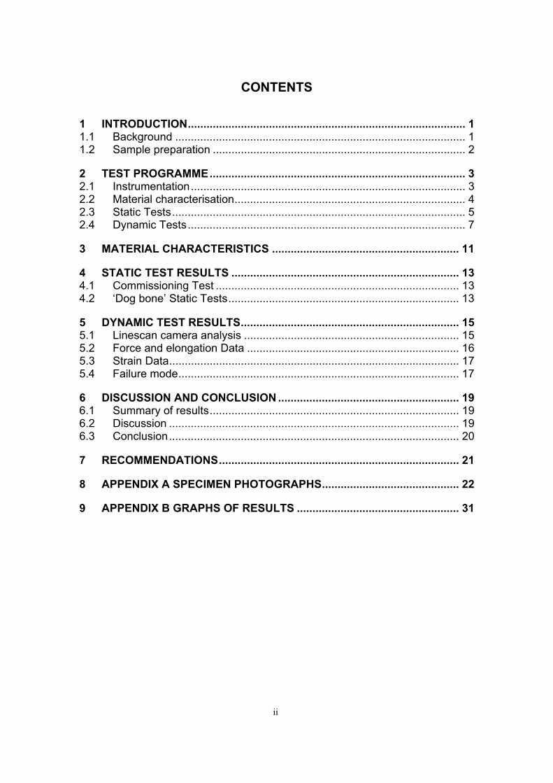
All strain gauges were located on the centre line of the specimen 30mm from each edge of the
weld, as shown in Figure 5.
3
30mm30mm
FES0508-04/2 Figure 5. Strain gauge locations
All dynamic tests were recorded with a high speed video system, suspended on a frame above
the specimen. The system utilises a high speed CCD camera head streaming frames of video to
solid state memory. For the commissioning test on specimen 5 the camera captured an area of
208 by 304 pixels in 8bit greyscale at a frame rate of 3800fps. This frame rate was found to be
more than required and the subsequent tests on specimens 4,7 and 8 were captured with an area
of 256 by 512 pixels with a frame rate of 2000fps.
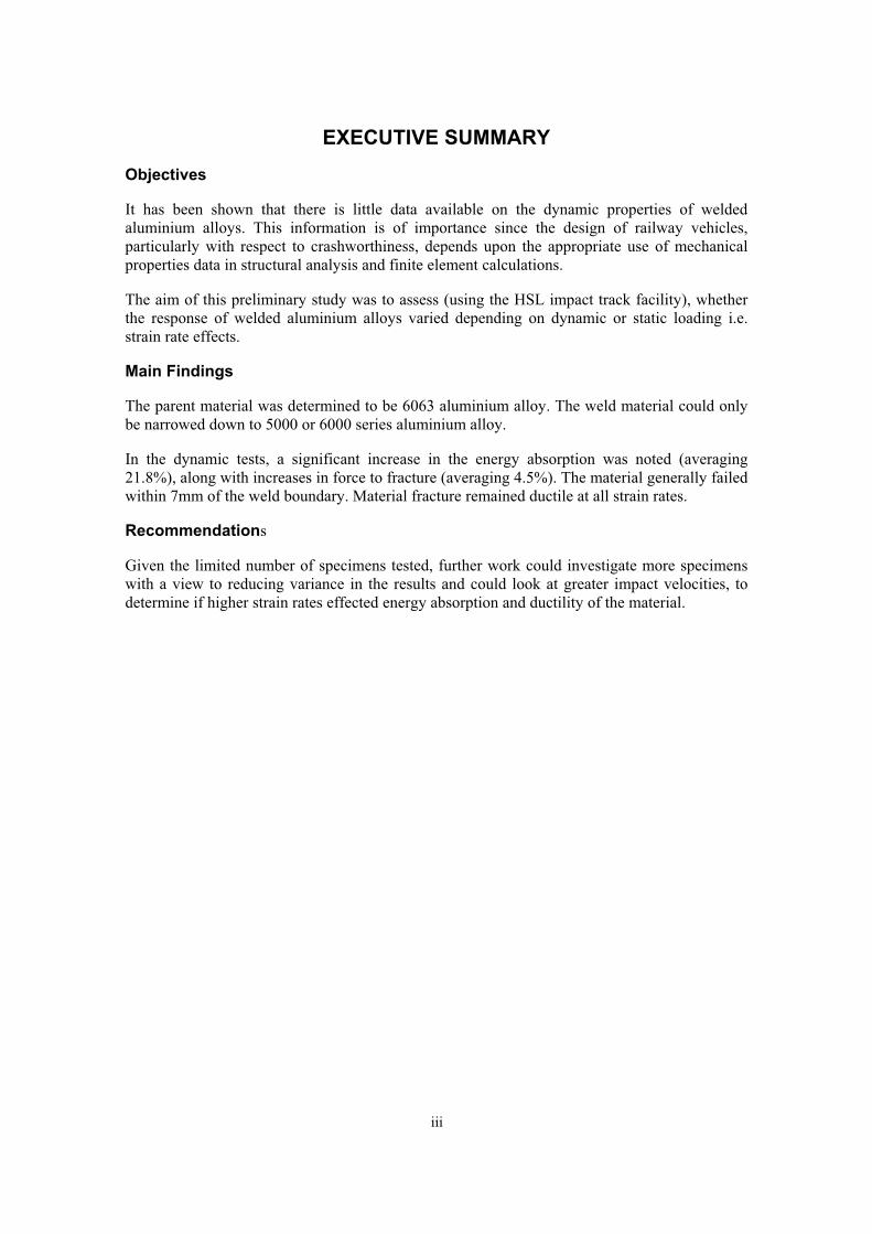
2.2 MATERIAL CHARACTERISATION
Quasi-static tensile tests were carried out on two parent samples and two weld samples
(transverse) taken from the outer skin of the side wall of the driving module section. The
specimens were machined with their longitudinal axis perpendicular to the extrusion direction in
the side wall sections of the module. In the case of the weld specimens, the weld was located in
the centre of the reduced gauge length. The tensile tests were carried out in accordance with BS
EN 895:1995 Destructive tests on welds in metallic materials – Transverse tensile test and BS
EN 10002-1:2001 Metallic Materials – Tensile Testing. The specimen geometry used is shown
in Figure 6.
25±0.1
11050
37
25
~240
25±0.1
11050
37
25
~240
Figure 6. Sheet tensile specimen geometry (all dimensions in mm).
The specimen thickness was approximately 2.5mm and both this and the gauge width were
measured at five points along the reduced length. An extensometer with a 50mm gauge length
was placed centrally on the reduced section to measure elongation. The tests were carried out
4
under position control in a servohydraulic test machine at a crosshead speed of 1.5mm/min,
increasing to 5mm/min following yielding.
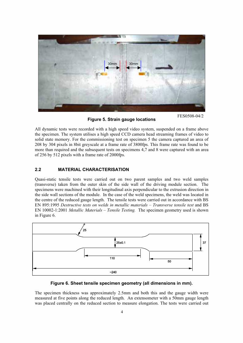
2.3 STATIC TESTS
The static tests were conducted using the specimen truck that was to be used for the dynamic
tests on the HSL Impact Track. This helped ensure similarity of test conditions between static
and dynamic tests. The specimen truck consists of a main body with slots in which an anvil
slides, Figure 7.
Figure 7. Blue specimen truck
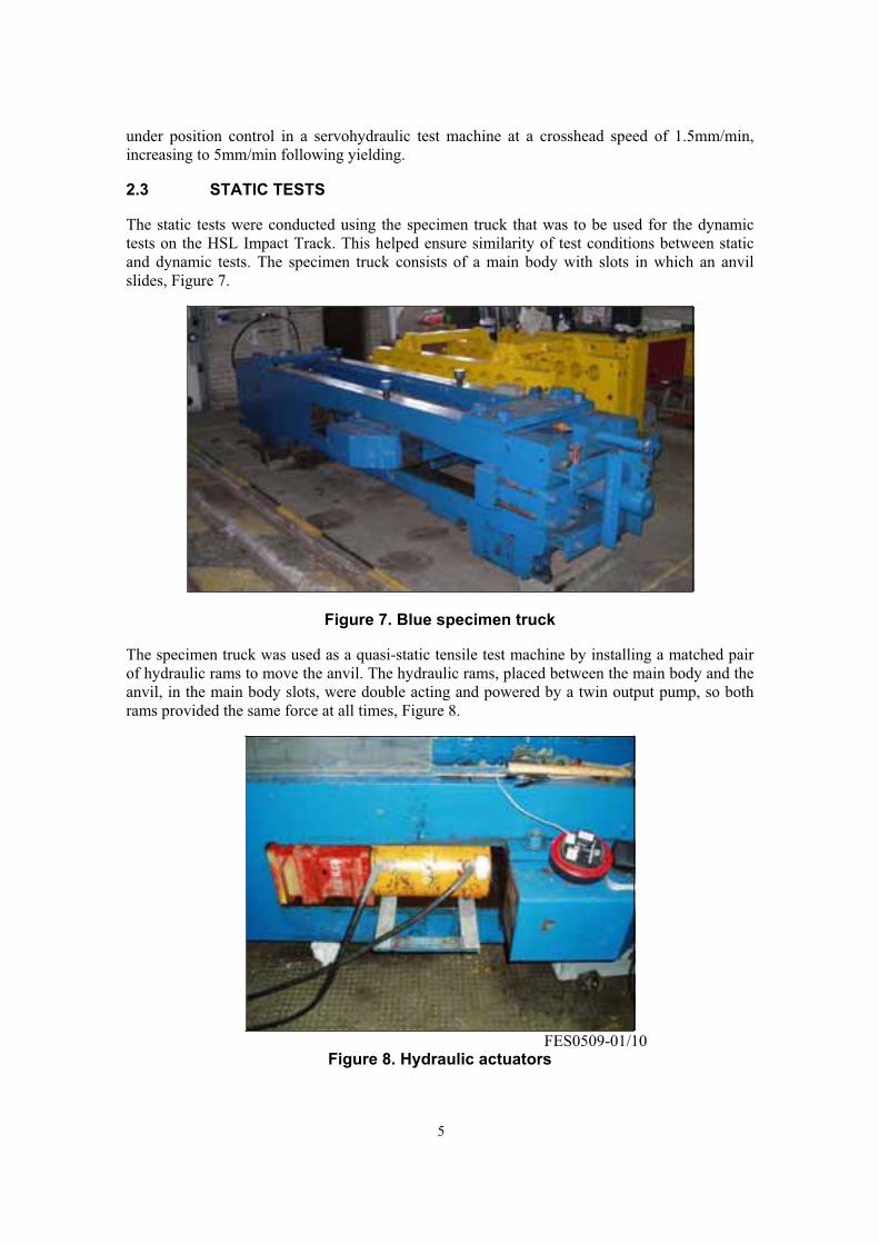
The specimen truck was used as a quasi-static tensile test machine by installing a matched pair
of hydraulic rams to move the anvil. The hydraulic rams, placed between the main body and the
anvil, in the main body slots, were double acting and powered by a twin output pump, so both
rams provided the same force at all times, Figure 8.
Figure 8. Hydraulic actuators FES0509-01/10
5

Each specimen was located inside the truck and fixed to the rigid end via a loadcell. The other
end of the specimen was attached to the sliding anvil
The elongation potentiometer was secured to the body of the sample truck with a large magnetic
base. The slider was connected to the moving anvil with another magnet. Figure 9 shows ‘dog
bone’ specimen number 1, in place. The potentiometer is visible in the upper left quadrant, and
the circular loadcell is shown at the right edge. The strain gauges can also be seen either side of
the central weld line.
Figure 9. Specimen number 1 in place in impact truck
FES0509-01/2
A schematic of the specimens, the method in which each was clamped and detailed dimensions
are shown in Figure 10.
6
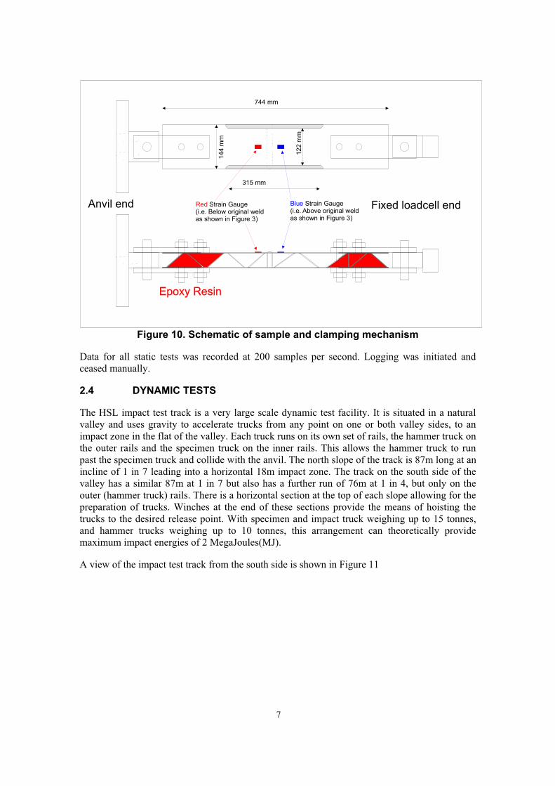
Anvil end Fixed loadcell end
744 mm
315 mm
12
2 m
m
14
4 m
m
Red Strain Gauge(i.e. Below original weldas shown in Figure 3)
Blue Strain Gauge(i.e. Above original weldas shown in Figure 3)
Figure 10. Schematic of sample and clamping mechanism
Data for all static tests was recorded at 200 samples per second. Logging was initiated and
ceased manually.
2.4 DYNAMIC TESTS
The HSL impact test track is a very large scale dynamic test facility. It is situated in a natural
valley and uses gravity to accelerate trucks from any point on one or both valley sides, to an
impact zone in the flat of the valley. Each truck runs on its own set of rails, the hammer truck on
the outer rails and the specimen truck on the inner rails. This allows the hammer truck to run
past the specimen truck and collide with the anvil. The north slope of the track is 87m long at an
incline of 1 in 7 leading into a horizontal 18m impact zone. The track on the south side of the
valley has a similar 87m at 1 in 7 but also has a further run of 76m at 1 in 4, but only on the
outer (hammer truck) rails. There is a horizontal section at the top of each slope allowing for the
preparation of trucks. Winches at the end of these sections provide the means of hoisting the
trucks to the desired release point. With specimen and impact truck weighing up to 15 tonnes,
and hammer trucks weighing up to 10 tonnes, this arrangement can theoretically provide
maximum impact energies of 2 MegaJoules(MJ).
A view of the impact test track from the south side is shown in Figure 11
7
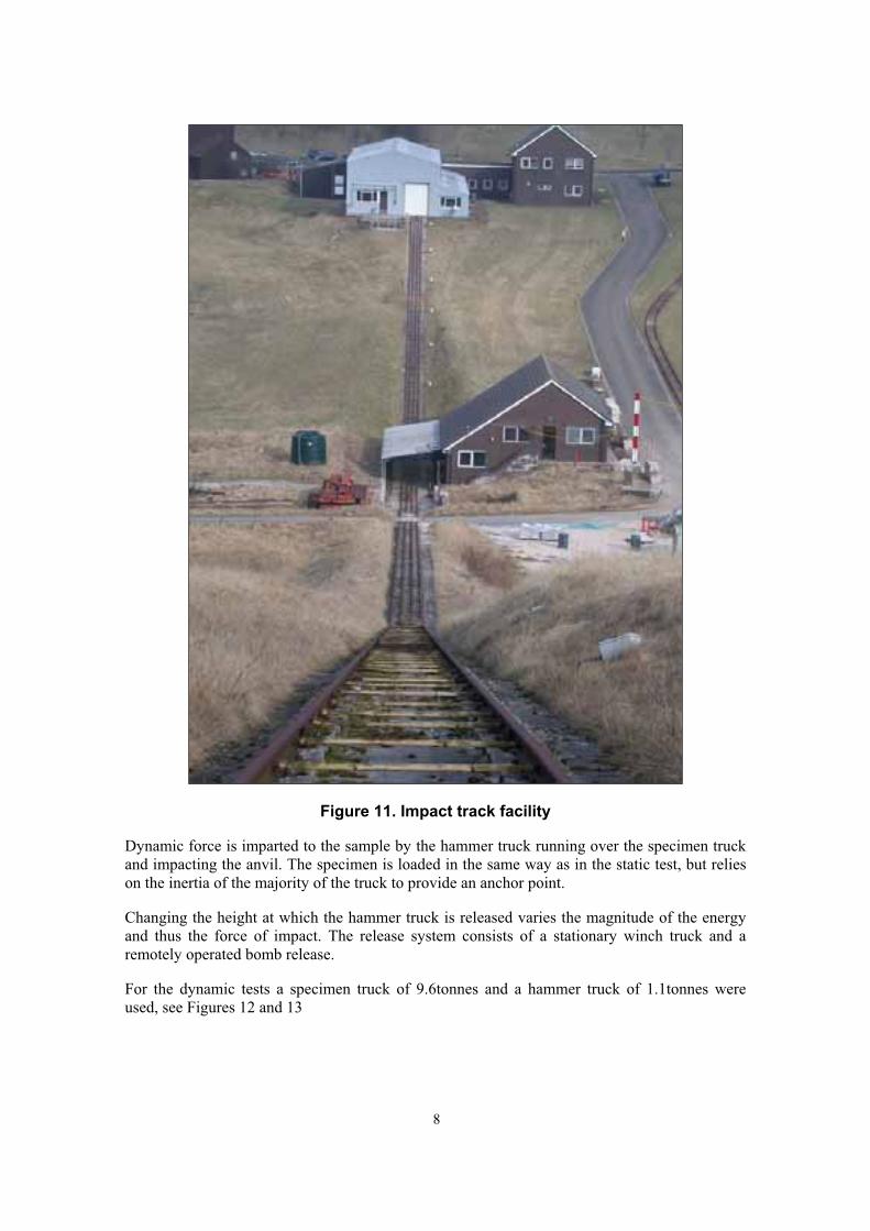
Figure 11. Impact track facility
Dynamic force is imparted to the sample by the hammer truck running over the specimen truck
and impacting the anvil. The specimen is loaded in the same way as in the static test, but relies
on the inertia of the majority of the truck to provide an anchor point.
Changing the height at which the hammer truck is released varies the magnitude of the energy
and thus the force of impact. The release system consists of a stationary winch truck and a
remotely operated bomb release.
For the dynamic tests a specimen truck of 9.6tonnes and a hammer truck of 1.1tonnes were
used, see Figures 12 and 13
8
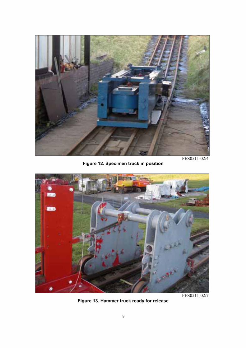
FES0511-02/4 Figure 12. Specimen truck in position
FES0511-02/7
Figure 13. Hammer truck ready for release
9

Data for all dynamic tests was recorded at 20,000 samples per second. A pencil lead breaker
circuit initiated logging automatically. The logging ceased after a duration of 1 second.
Three dynamic tests were conducted with the weld facing upwards ( i.e. towards the high speed
camera ), the final test utilised a sample rotated through 90 degrees in order to observe the
failure mechanism from a side elevation.
10
3 MATERIAL CHARACTERISTICS
3.1 TENSILE PROPERTIES
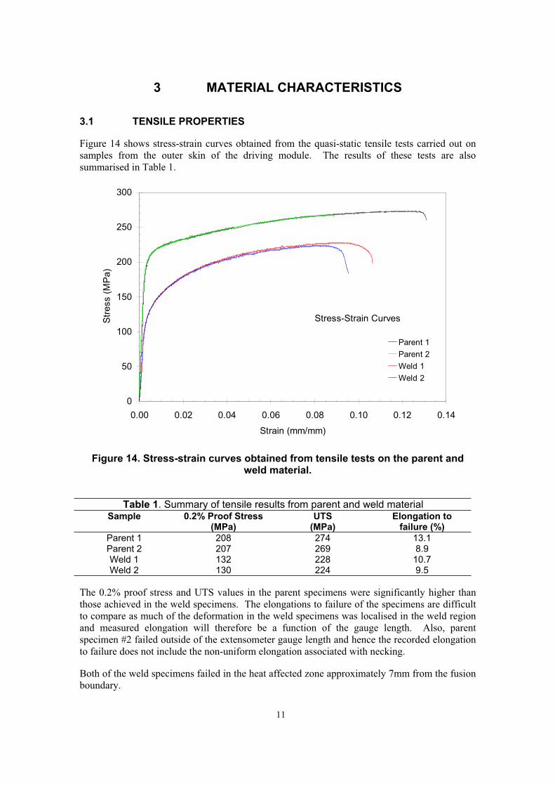
Figure 14 shows stress-strain curves obtained from the quasi-static tensile tests carried out on
samples from the outer skin of the driving module. The results of these tests are also
summarised in Table 1.
Stress-Strain Curves
0
50
100
150
200
250
300
0.00 0.02 0.04 0.06 0.08 0.10 0.12 0.14
Strain (mm/mm)
Str
ess (
MP
a)
Parent 1
Parent 2
Weld 1
Weld 2
Figure 14. Stress-strain curves obtained from tensile tests on the parent and weld material.
Table 1. Summary of tensile results from parent and weld materialSample 0.2% Proof Stress
(MPa)UTS
(MPa)Elongation to
failure (%)
Parent 1 208 274 13.1Parent 2 207 269 8.9Weld 1 132 228 10.7Weld 2 130 224 9.5
The 0.2% proof stress and UTS values in the parent specimens were significantly higher than
those achieved in the weld specimens. The elongations to failure of the specimens are difficult
to compare as much of the deformation in the weld specimens was localised in the weld region
and measured elongation will therefore be a function of the gauge length. Also, parent
specimen #2 failed outside of the extensometer gauge length and hence the recorded elongation
to failure does not include the non-uniform elongation associated with necking.
Both of the weld specimens failed in the heat affected zone approximately 7mm from the fusion
boundary.
11
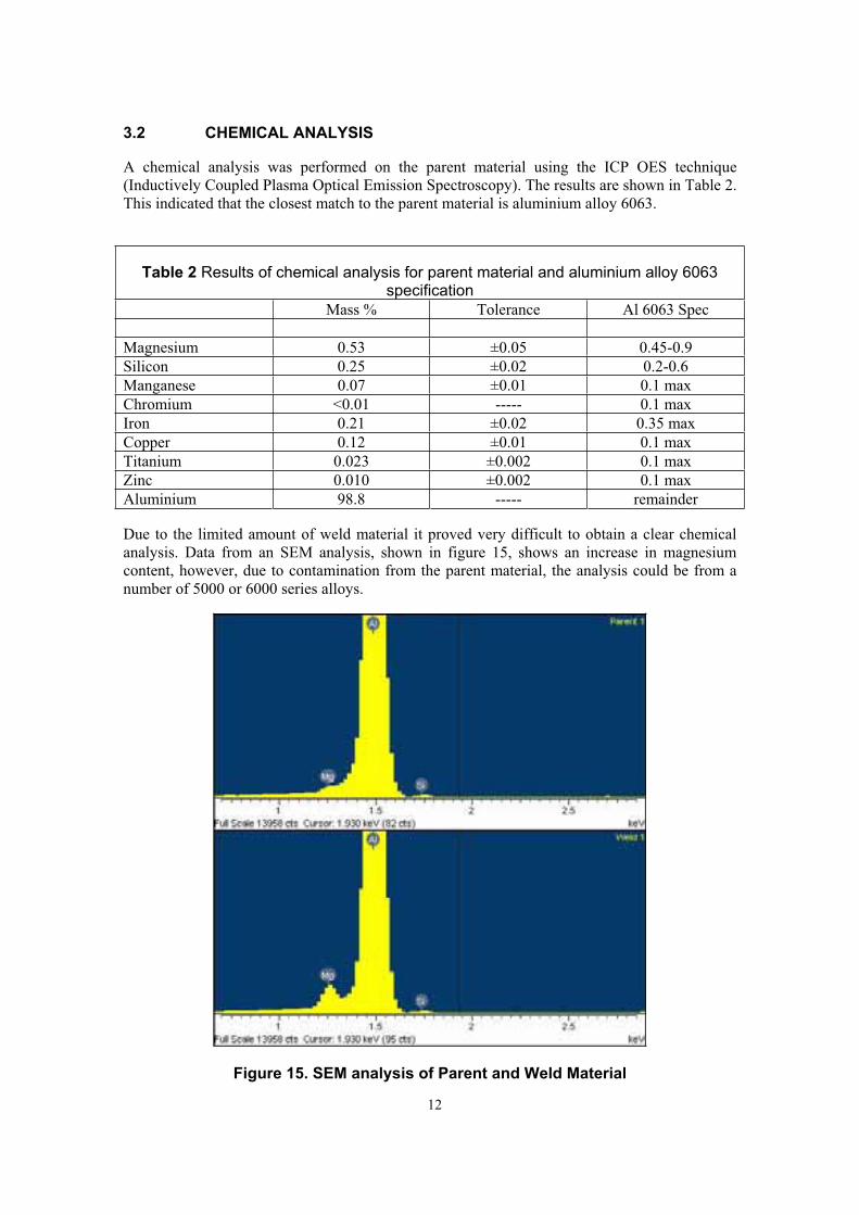
3.2 CHEMICAL ANALYSIS
A chemical analysis was performed on the parent material using the ICP OES technique
(Inductively Coupled Plasma Optical Emission Spectroscopy). The results are shown in Table 2.
This indicated that the closest match to the parent material is aluminium alloy 6063.
Table 2 Results of chemical analysis for parent material and aluminium alloy 6063 specification
Mass % Tolerance Al 6063 Spec
Magnesium 0.53 ±0.05 0.45-0.9
Silicon 0.25 ±0.02 0.2-0.6
Manganese 0.07 ±0.01 0.1 max
Chromium <0.01 ----- 0.1 max
Iron 0.21 ±0.02 0.35 max
Copper 0.12 ±0.01 0.1 max
Titanium 0.023 ±0.002 0.1 max
Zinc 0.010 ±0.002 0.1 max
Aluminium 98.8 ----- remainder
Due to the limited amount of weld material it proved very difficult to obtain a clear chemical
analysis. Data from an SEM analysis, shown in figure 15, shows an increase in magnesium
content, however, due to contamination from the parent material, the analysis could be from a
number of 5000 or 6000 series alloys.
Figure 15. SEM analysis of Parent and Weld Material
12
4 STATIC TEST RESULTS
4.1 COMMISSIONING TEST
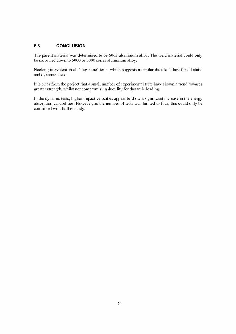
The commissioning test was conducted on a rectangular specimen 144mm wide. The result of
this test was a specimen failure at one of the clamping bolt holes, see Figure A1(b).
Instrumentation for this test did not include strain gauges, however force and elongation were
successfully recorded.
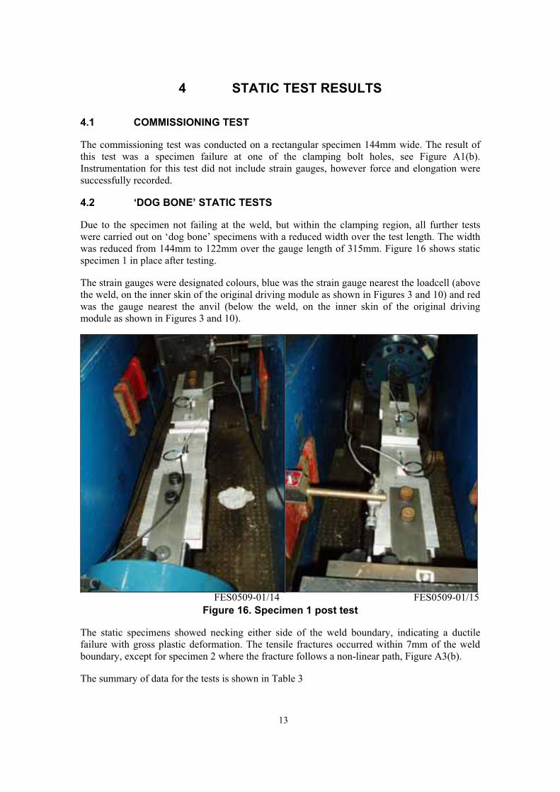
4.2 ‘DOG BONE’ STATIC TESTS
Due to the specimen not failing at the weld, but within the clamping region, all further tests
were carried out on ‘dog bone’ specimens with a reduced width over the test length. The width
was reduced from 144mm to 122mm over the gauge length of 315mm. Figure 16 shows static
specimen 1 in place after testing.
The strain gauges were designated colours, blue was the strain gauge nearest the loadcell (above
the weld, on the inner skin of the original driving module as shown in Figures 3 and 10) and red
was the gauge nearest the anvil (below the weld, on the inner skin of the original driving
module as shown in Figures 3 and 10).
Figure 16. Specimen 1 post test
FES0509-01/14 FES0509-01/15
The static specimens showed necking either side of the weld boundary, indicating a ductile
failure with gross plastic deformation. The tensile fractures occurred within 7mm of the weld
boundary, except for specimen 2 where the fracture follows a non-linear path, Figure A3(b).
The summary of data for the tests is shown in Table 3
13

Table 3 Summary of data for static tests
Elongation (mm) Energy Absorbed
(J)
Test
Specimen
Temperature Maximum
Force (kN)
At Weld
Failure1At Ultimate
Failure
To Weld
Failure1Total
6(Commissioning)
14oC 198.2 12.2 NA NA NA
1 14oC NA 11.4 34.3 NA NA
2 14oC 171.9 11.5 34.1 1510 1708
3 14oC 171.3 11.7 36.0 1401 17171: Weld failure is defined as the event that causes the first significant decrease in tensile strength
Elongation & Force Histories, Energy and strain gauge graphs are shown in Appendix B
Figures B1 to B3 show Force and Elongation histories for specimens 6,2 and 3
The blue trace shows the force applied over time to the specimen and the red trace shows the
corresponding elongation over time of the specimen. The green line is zero. Figures B2 and B3
show drop out in force and corresponding elongation, due to the force being manually reduced
to allow inspection of the condition of the specimen.
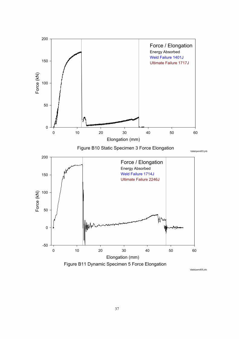
Figures B8 to B10 show Force against Elongation for specimens 6,2 and 3
The trace shows force plotted against elongation thus removing the dependency of time and
hence the area under the graph gives the energy absorbed. The first area indicates the portion to
first and second failures, which occur at substantially the same time. The final ramp indicates
the specimen rotating about the remaining two webs as the specimen tries to straighten out, until
ultimate failure.
Figures B15 to B17 show Strain Gauge histories for specimens 1,2 and 3
The blue trace shows the strain recorded by the blue strain gauge over time, the red trace shows
the corresponding red gauge. The grey trace shows the force history applied to the specimen.
The green line is zero.
Figure B15 (specimen 1) shows no force data, as the force was not recorded for that test.
Flat tops indicate that the gauge has reached the maximum value it can record. Data recorded
after the flat top event is still valid, however, the gauge may have delaminated during the event.
Modifications to the logging system were made in an attempt to rectify this in subsequent tests.
The phase difference between the two gauge traces indicates that the blue gauge records a
greater strain before that of the red gauge, prior to delamination. This indicates that the section
of material to the loadcell end (above the weld, on the inner skin of the original driving module)
is weaker than that of the anvil side (below the weld, on the inner skin of the driving module).
As these tests are quasi-static the time base is not directly relevant but indicates the sequence of
events.
14

5 DYNAMIC TEST RESULTS
5.1 HIGH SPEED CAMERA ANALYSIS
5.1.1 Impact Velocity
To calculate the impact speed of the impact truck a section of it carried markers. This section
provided a 113mm calibrated length. This allowed subsequent analysis and calibration of each
frame to determine the input velocity. Figure 16 shows an example of the analysis.
113mm
Frame 260 (0.0ms) Frame 330 (18.41ms) Frame 400 (36.82ms)
64.9mm
129.2mm
Figure 17. High speed camera velocity analysis for Specimen 5
As seen in Figure 17, frame 260 shows the calibrated section. Frames 330 and 400 show the
passage of the impact truck and how the displacement was measured, from which the velocity
was calculated.
Table 4 Analysis of high speed video for input velocity
Frame Distance travelled (mm) Velocity (m/s)
260 0 NA
330 64.9 3.53
400 129.2 3.51
5.1.2 Sample Elongation
A similar technique to that described in 5.1.1 was used to determine the elongation of the
sample during loading. Figure 17 shows an example of the analysis.
15
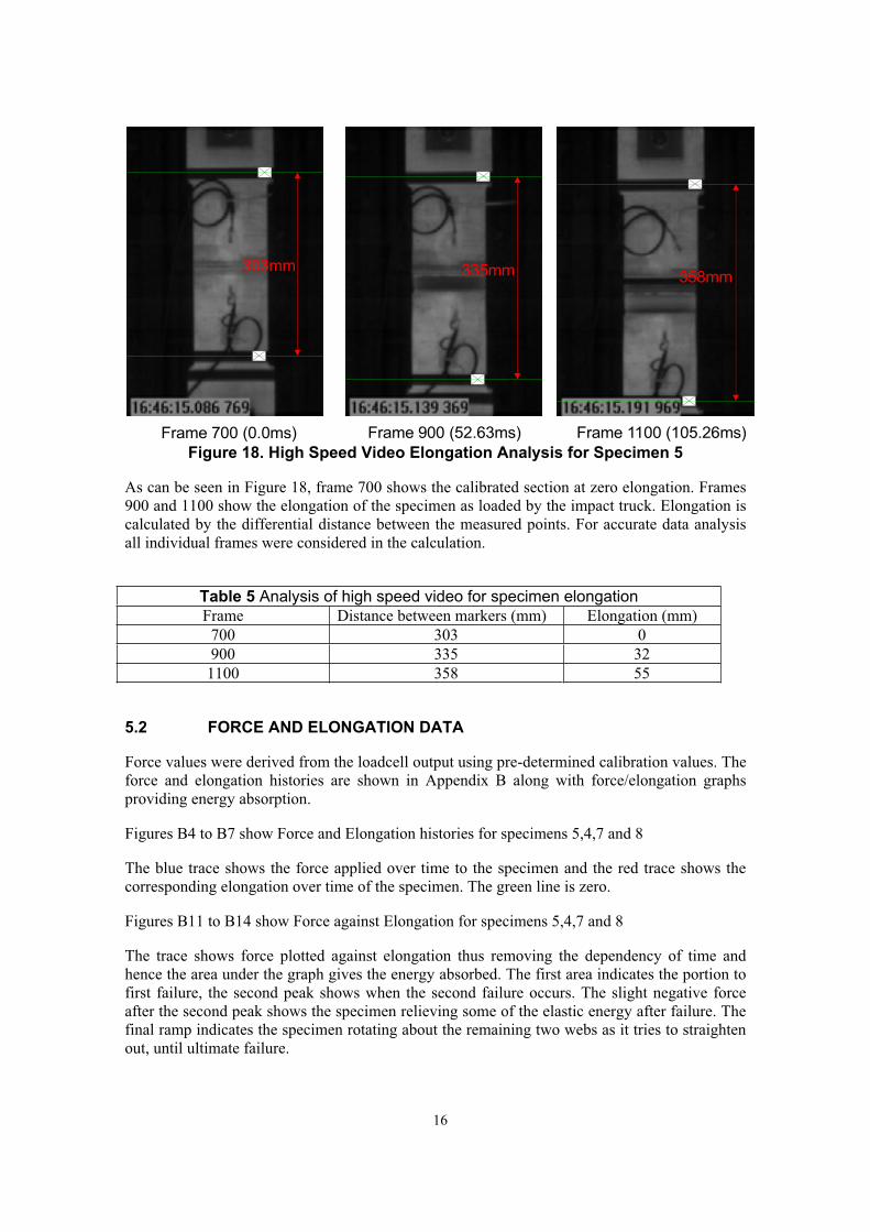
303mm 335mm 358mm
Frame 700 (0.0ms) Frame 900 (52.63ms) Frame 1100 (105.26ms)
Figure 18. High Speed Video Elongation Analysis for Specimen 5
As can be seen in Figure 18, frame 700 shows the calibrated section at zero elongation. Frames
900 and 1100 show the elongation of the specimen as loaded by the impact truck. Elongation is
calculated by the differential distance between the measured points. For accurate data analysis
all individual frames were considered in the calculation.
Table 5 Analysis of high speed video for specimen elongation
Frame Distance between markers (mm) Elongation (mm)
700 303 0
900 335 32
1100 358 55
5.2 FORCE AND ELONGATION DATA
Force values were derived from the loadcell output using pre-determined calibration values. The
force and elongation histories are shown in Appendix B along with force/elongation graphs
providing energy absorption.
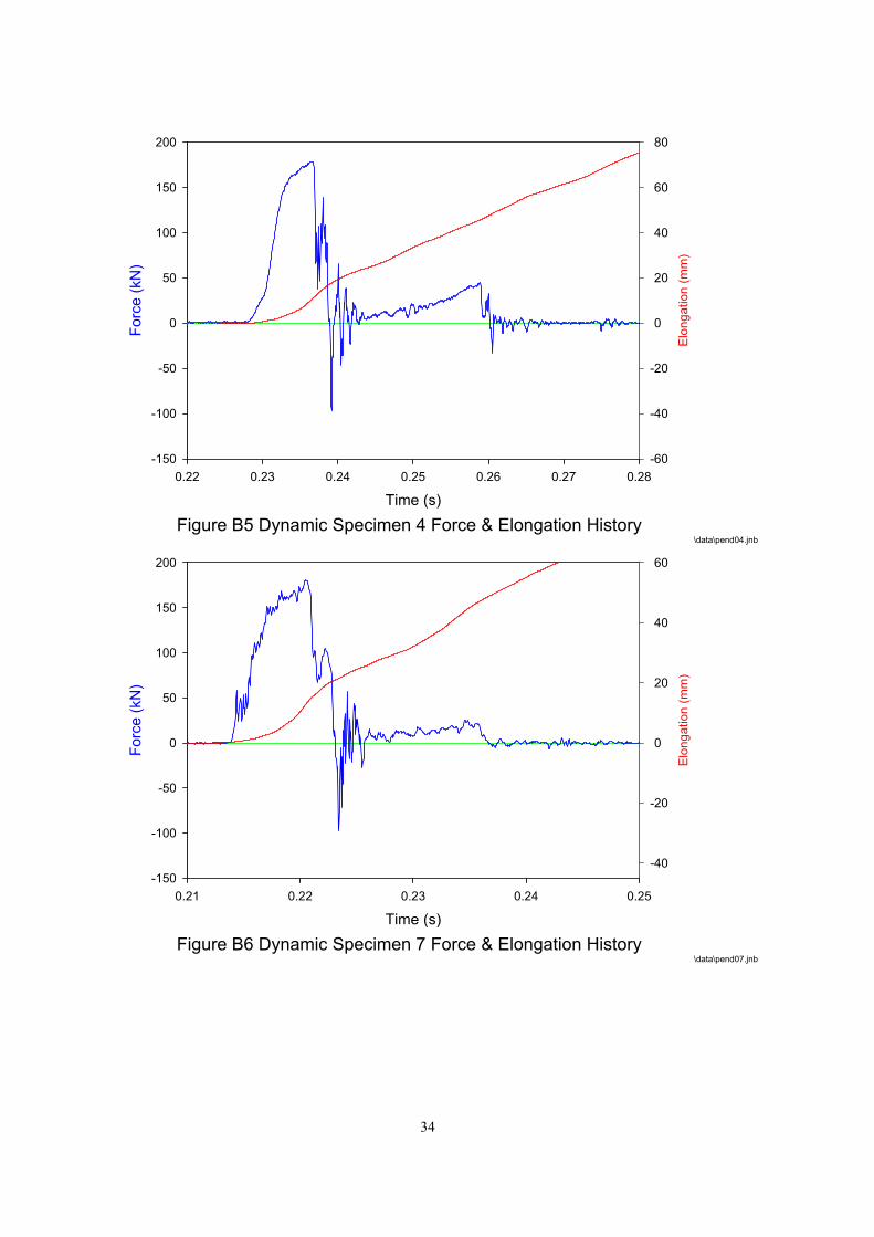
Figures B4 to B7 show Force and Elongation histories for specimens 5,4,7 and 8
The blue trace shows the force applied over time to the specimen and the red trace shows the
corresponding elongation over time of the specimen. The green line is zero.
Figures B11 to B14 show Force against Elongation for specimens 5,4,7 and 8
The trace shows force plotted against elongation thus removing the dependency of time and
hence the area under the graph gives the energy absorbed. The first area indicates the portion to
first failure, the second peak shows when the second failure occurs. The slight negative force
after the second peak shows the specimen relieving some of the elastic energy after failure. The
final ramp indicates the specimen rotating about the remaining two webs as it tries to straighten
out, until ultimate failure.
16
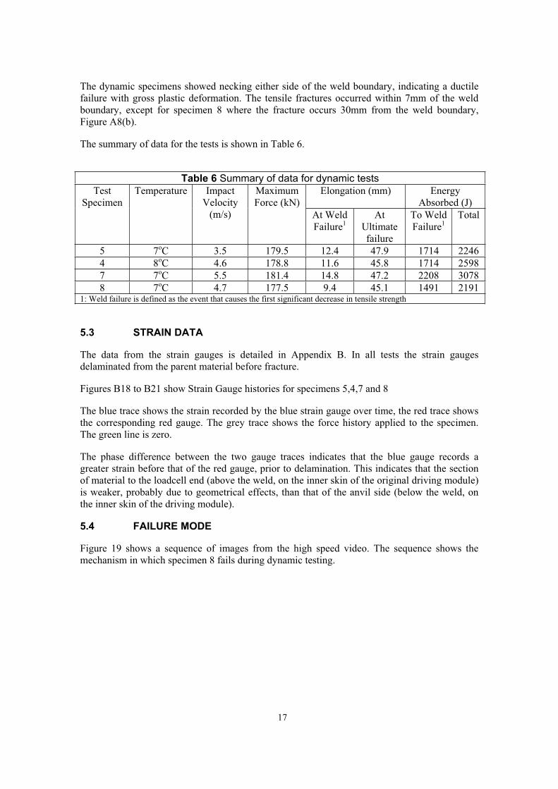
The dynamic specimens showed necking either side of the weld boundary, indicating a ductile
failure with gross plastic deformation. The tensile fractures occurred within 7mm of the weld
boundary, except for specimen 8 where the fracture occurs 30mm from the weld boundary,
Figure A8(b).
The summary of data for the tests is shown in Table 6.
Table 6 Summary of data for dynamic tests
Elongation (mm) Energy
Absorbed (J)
Test
Specimen
Temperature Impact
Velocity
(m/s)
Maximum
Force (kN)
At Weld
Failure1At
Ultimate
failure
To Weld
Failure1Total
5 7oC 3.5 179.5 12.4 47.9 1714 2246
4 8oC 4.6 178.8 11.6 45.8 1714 2598
7 7oC 5.5 181.4 14.8 47.2 2208 3078
8 7oC 4.7 177.5 9.4 45.1 1491 21911: Weld failure is defined as the event that causes the first significant decrease in tensile strength
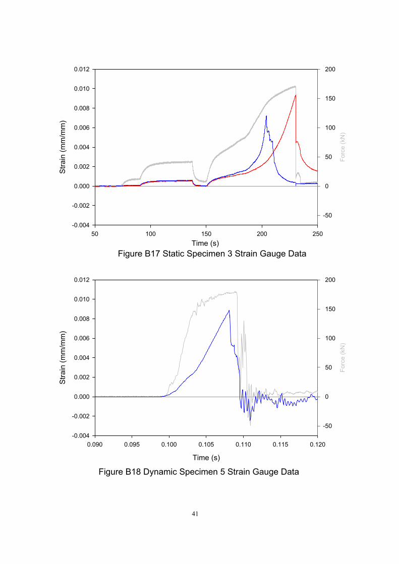
5.3 STRAIN DATA
The data from the strain gauges is detailed in Appendix B. In all tests the strain gauges
delaminated from the parent material before fracture.
Figures B18 to B21 show Strain Gauge histories for specimens 5,4,7 and 8
The blue trace shows the strain recorded by the blue strain gauge over time, the red trace shows
the corresponding red gauge. The grey trace shows the force history applied to the specimen.
The green line is zero.
The phase difference between the two gauge traces indicates that the blue gauge records a
greater strain before that of the red gauge, prior to delamination. This indicates that the section
of material to the loadcell end (above the weld, on the inner skin of the original driving module)
is weaker, probably due to geometrical effects, than that of the anvil side (below the weld, on
the inner skin of the driving module).
5.4 FAILURE MODE
Figure 19 shows a sequence of images from the high speed video. The sequence shows the
mechanism in which specimen 8 fails during dynamic testing.
17
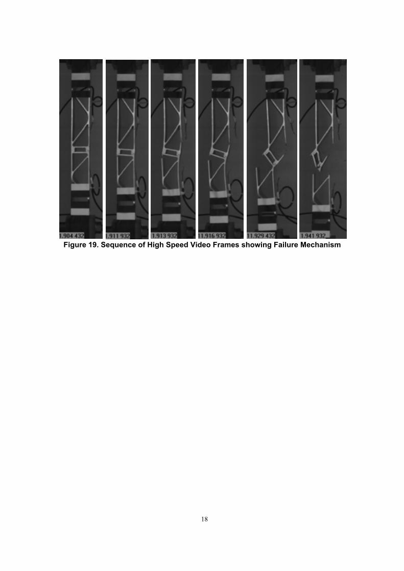
Figure 19. Sequence of High Speed Video Frames showing Failure Mechanism
18

6 DISCUSSION AND CONCLUSION
6.1 SUMMARY OF RESULTS
Table 7 shows a summary of the results.
Table 7 Summary of results
Specimen Type Maximum Force
(kN)
Elongation at Weld
Failure (mm)
Energy absorbed at
Weld Failure (J)
Averaged Averaged Averaged
1 Static NA 11.4 NA
2 Static 171.9 11.5 1510
3 Static 171.3 171.6
11.7
11.5
14011456
5 Dynamic 179.5 12.4 1714
4 Dynamic 178.8 11.6 1682
7 Dynamic 181.4 14.8 2208
8 Dynamic 177.5
179.3
9.4
12.1
1491
1774
It can be noted that:
the dynamic tests caused failure at greater forces than the static tests, on average 4.5%
the elongation averages for the dynamic tests are apparently 5.2 % greater than for the
static,
there is a significant increase in the energy absorption in dynamic loading, on average
21.8%. This increase is due in part to the increase in force to failure, but also due to the
shape of the force elongation curve (for example compare Figure B10 to B11).
there appears to be a significant increase in the energy absorption capabilities for higher
impact velocities. Due to the limited number of tests, however, this could be a factor of
statistical variance.
6.2 DISCUSSION
The mode of failure was fairly consistent, and the sequence of failure can be seen in Figure 18.
The first fracture to occur was usually less than 7mm from the weld boundary. The second
fracture to occur was on the opposite face and other side of the interlock, again usually less than
7mm from the weld boundary. This event has been referred to as weld failure. The third fracture
was caused by severe rotation of the area near the interlock as the specimen tries to straighten
out. The process can be seen in Figure 18. The exceptions to this were specimen 2 (static),
where the fracture follows a non-linear path, Figure A3(b), and specimen 8 (dynamic) where the
second fracture occurs 30mm from the weld boundary, Figure A8(b)
The data from the strain gauges indicates that the section of material to the loadcell end (above
the weld, on the inner skin of the original driving module) is weaker, probably due to
geometrical effects, than that of the anvil side (below the weld, on the inner skin of the driving
module). Both areas in which the strain gauges were placed experienced gross plastic
deformation
19
6.3 CONCLUSION
The parent material was determined to be 6063 aluminium alloy. The weld material could only
be narrowed down to 5000 or 6000 series aluminium alloy.
Necking is evident in all ‘dog bone’ tests, which suggests a similar ductile failure for all static
and dynamic tests.
It is clear from the project that a small number of experimental tests have shown a trend towards
greater strength, whilst not compromising ductility for dynamic loading.
In the dynamic tests, higher impact velocities appear to show a significant increase in the energy
absorption capabilities. However, as the number of tests was limited to four, this could only be
confirmed with further study.
20

7 RECOMMENDATIONS
This was a preliminary study and, given the limited number of specimens tested, further work
could utilise more specimens with a view to reducing variance in the results.
Further investigation into higher impact velocities could determine if higher strain rates result in
greater energy absorption and a reduction in the ductility of the material. Impact velocities on
the HSL impact test track can be increased up to 30m/s.
21

8 APPENDIX A SPECIMEN PHOTOGRAPHS
22
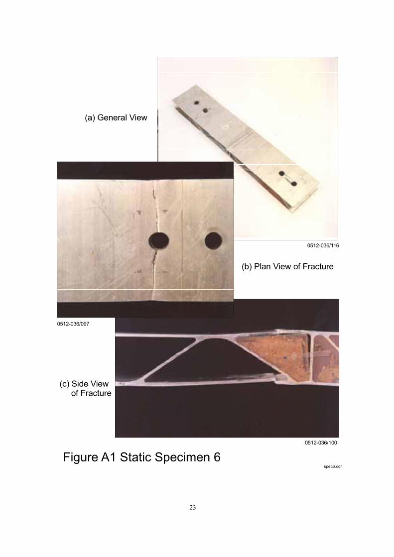
Figure A1 Static Specimen 6spec6.cdr
0512-036/100
0512-036/097
0512-036/116
(a) General View
(b) Plan View of Fracture
(c) Side View of Fracture
23
Figure A2 Static Specimen 1spec1.cdr
0512-036/072
0512-036/070
0512-036/111
(a) General View
(b) Plan View of Fracture
(c) Side View of Fracture
24

0512-036/077
0512-036/075
0512-036/112
(a) General View
(b) Plan View of Fracture
(c) Side View of Fracture
Figure A3 Static Specimen 2spec2.cdr
25
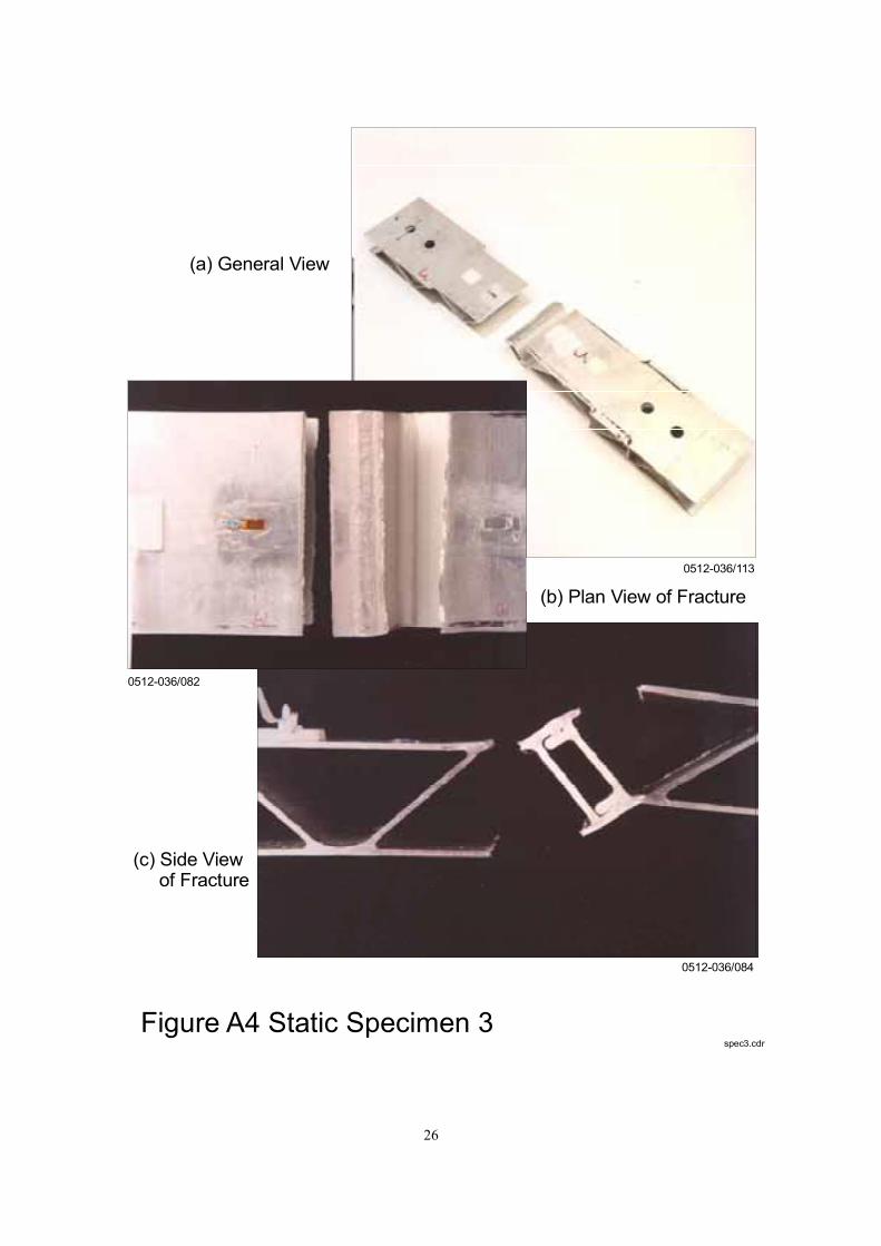
Figure A4 Static Specimen 3spec3.cdr
0512-036/082
0512-036/113
0512-036/084
(a) General View
(b) Plan View of Fracture
(c) Side View of Fracture
26

Figure A5 Dynamic Specimen 5spec5.cdr
0512-036/094
0512-036/092
0512-036/114
(a) General View
(b) Plan View of Fracture
(c) Side View of Fracture
27
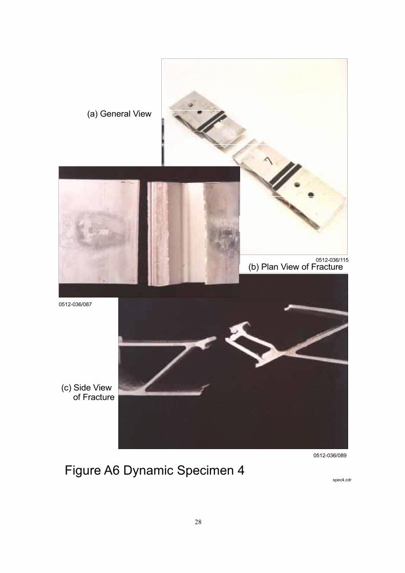
Figure A6 Dynamic Specimen 4spec4.cdr
0512-036/089
0512-036/087
0512-036/115
(a) General View
(b) Plan View of Fracture
(c) Side View of Fracture
28

Figure A7 Dynamic Specimen 7spec7.cdr
0512-036/104
0512-036/102
0512-036/117
(a) General View
(b) Plan View of Fracture
(c) Side View of Fracture
29
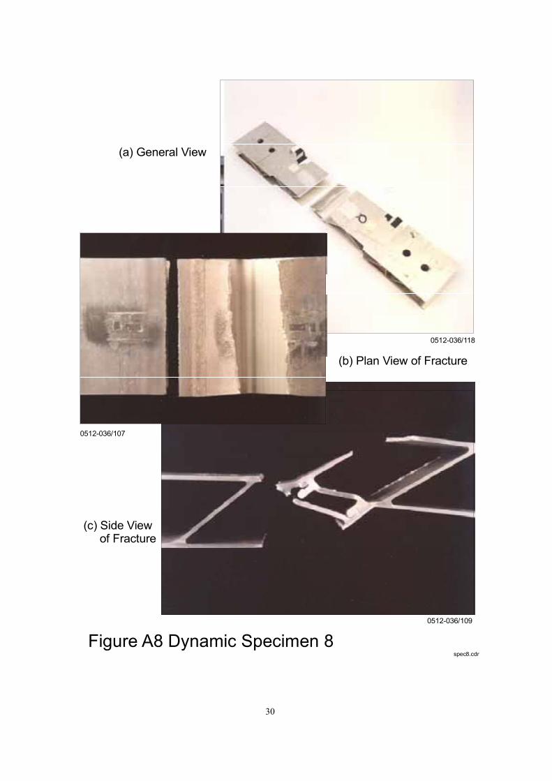
Figure A8 Dynamic Specimen 8spec8.cdr
0512-036/109
0512-036/107
0512-036/118
(a) General View
(b) Plan View of Fracture
(c) Side View of Fracture
30

9 APPENDIX B GRAPHS OF RESULTS
31
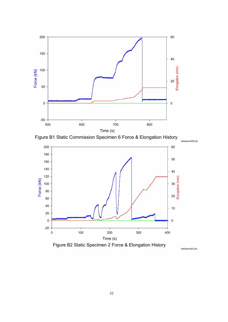
Figure B1 Static Commission Specimen 6 Force & Elongation History
Time (s)
500 600 700 800
Fo
rce
(kN
)
-50
0
50
100
150
200
0
20
40
60
Elo
nga
tio
n (
mm
)
\data\pend06.jnb
0
10
20
30
40
50
60
-20
0
20
40
60
80
100
120
140
160
180
200
Figure B2 Static Specimen 2 Force & Elongation History
Time (s)
Elo
ng
atio
n (
mm
)
Fo
rce
(kN
)
0 100 200 300 400
\data\pend02.jnb
32
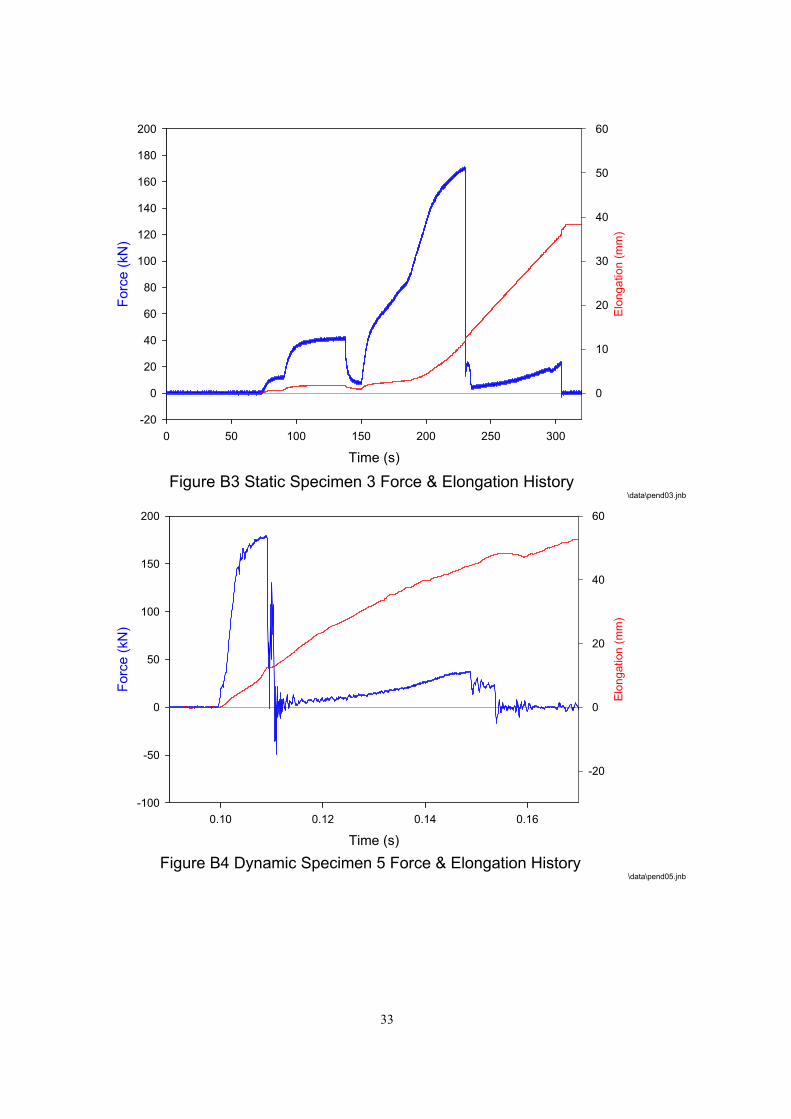
Figure B3 Static Specimen 3 Force & Elongation History
Time (s)
0 50 100 150 200 250 300
Forc
e (
kN
)
-20
0
20
40
60
80
100
120
140
160
180
200
0
10
20
30
40
50
60
Elo
nga
tion (
mm
)
\data\pend03.jnb
Figure B4 Dynamic Specimen 5 Force & Elongation History
Time (s)
0.10 0.12 0.14 0.16
Forc
e (
kN
)
-100
-50
0
50
100
150
200
-20
0
20
40
60
Elo
ng
atio
n (
mm
)
\data\pend05.jnb
33
-150
-100
-50
0
50
100
150
200
-60
-40
-20
0
20
40
60
80
Figure B6 Dynamic Specimen 7 Force & Elongation History
Time (s)
0.21 0.22 0.23 0.24 0.25
Forc
e (
kN
)
-150
-100
-50
0
50
100
150
200
Elo
ng
atio
n (
mm
)
-40
-20
0
20
40
60
\data\pend07.jnb
Figure B5 Dynamic Specimen 4 Force & Elongation History
Time (s)
Elo
ng
atio
n (
mm
)
Fo
rce
(kN
)
0.22 0.23 0.24 0.25 0.26 0.27 0.28
\data\pend04.jnb
34
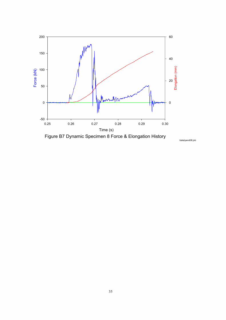
Figure B7 Dynamic Specimen 8 Force & Elongation History
Time (s)
0.25 0.26 0.27 0.28 0.29 0.30
Fo
rce
(kN
)
-50
0
50
100
150
200
0
20
40
60
Elo
nga
tio
n (
mm
)
\data\pend08.jnb
35

Force / ElongationEnergy Absorbed 1812J
Elongation (mm)
0 10 20 30 40 50 60
Fo
rce
(kN
)
0
50
100
150
200
Figure B8 Static Commission Specimen 6 Force Elongation\data\pend06.jnb
Force / ElongationEnergy Absorbed
To Weld Failure 1510J
0
20
40
60
80
100
120
140
160
180
200
To Ultimate Failure 1708J
Elongation (mm)
Fo
rce
(kN
)
0 10 20 30 40 50 60
Figure B9 Static Specimen 2 Force Elongation\data\pend02.jnb
36
Force / ElongationEnergy Absorbed
Weld Failure 1401J
0
50
100
150
200
Ultimate Failure 1717J
Elongation (mm)
Fo
rce
(kN
)
0 10 20 30 40 50 60
Figure B10 Static Specimen 3 Force Elongation\data\pend03.jnb
Force / ElongationEnergy Absorbed
Weld Failure 1714J
-50
0
50
100
150
200
Ultimate Failure 2246J
Elongation (mm)
Fo
rce
(kN
)
0 10 20 30 40 50 60
Figure B11 Dynamic Specimen 5 Force Elongation\data\pend05.jnb
37

Force / ElongationEnergy Absorbed
Weld Failure 1682J
-50
0
50
100
150
200
Ultimate Failure 2598J
Elongation (mm)
Fo
rce
(kN
)
0 10 20 30 40 50 60
Figure B12 Dynamic Specimen 4 Force Elongation\data\pend04.jnb
Force / ElongationEnergy Absorbed
Weld Failure 2208J
-50
0
50
100
150
200
Ultimate Failure 3078J
Elongation (mm)
Fo
rce
(kN
)
0 10 20 30 40 50 60
Figure B13 Dynamic Specimen 7 Force Elongation\data\pend07.jnb
38
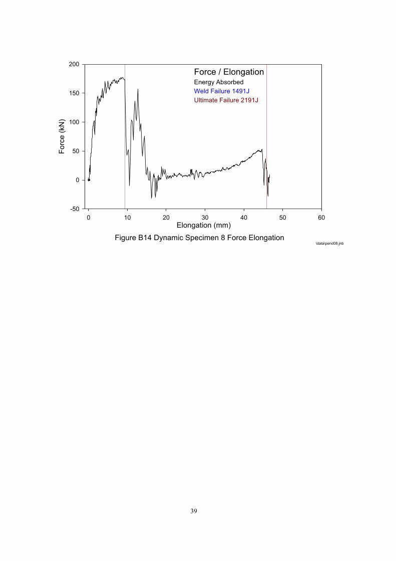
Force / ElongationEnergy Absorbed
Weld Failure 1491J
-50
0
50
100
150
200
Ultimate Failure 2191J
Elongation (mm)
Forc
e (
kN
)
0 10 20 30 40 50 60
Figure B14 Dynamic Specimen 8 Force Elongation\data\pend08.jnb
39
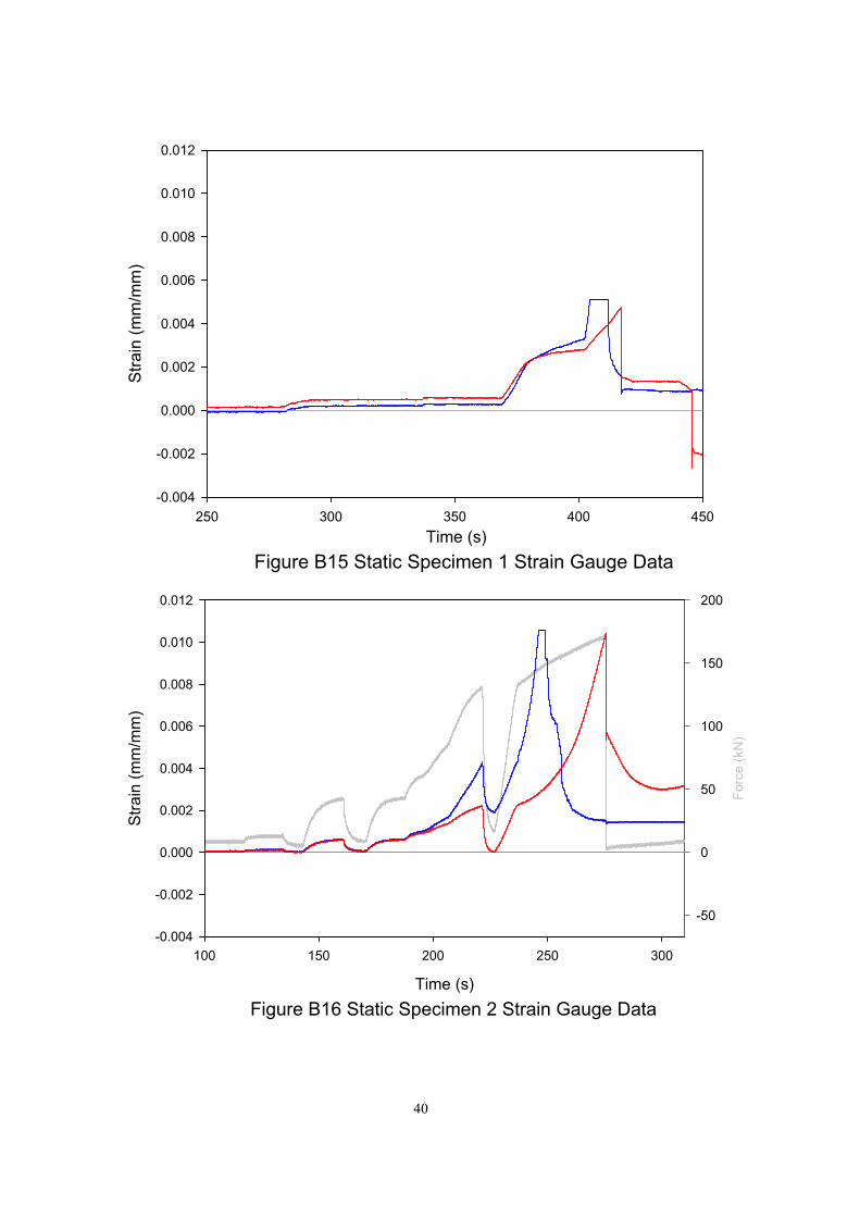
Figure B15 Static Specimen 1 Strain Gauge Data
Time (s)
250 300 350 400 450
Str
ain
(m
m/m
m)
-0.004
-0.002
0.000
0.002
0.004
0.006
0.008
0.010
0.012
Figure B16 Static Specimen 2 Strain Gauge Data
Time (s)
100 150 200 250 300
Forc
e (
kN
)
-50
0
50
100
150
200
Str
ain
(m
m/m
m)
-0.004
-0.002
0.000
0.002
0.004
0.006
0.008
0.010
0.012
40
Time (s)
50 100 150 200 250
Forc
e (
kN
)
-50
0
50
100
150
200S
tra
in (
mm
/mm
)
-0.004
-0.002
0.000
0.002
0.004
0.006
0.008
0.010
0.012
Figure B17 Static Specimen 3 Strain Gauge Data
Figure B18 Dynamic Specimen 5 Strain Gauge Data
Time (s)
0.090 0.095 0.100 0.105 0.110 0.115 0.120
Forc
e (
kN
)
-50
0
50
100
150
200
Str
ain
(m
m/m
m)
-0.004
-0.002
0.000
0.002
0.004
0.006
0.008
0.010
0.012
41
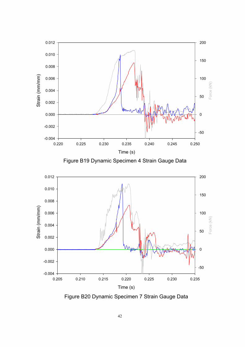
Figure B19 Dynamic Specimen 4 Strain Gauge Data
Time (s)
0.220 0.225 0.230 0.235 0.240 0.245 0.250
Forc
e (
kN
)
-50
0
50
100
150
200S
train
(m
m/m
m)
-0.004
-0.002
0.000
0.002
0.004
0.006
0.008
0.010
0.012
-50
0
50
100
150
200
-0.004
-0.002
0.000
0.002
0.004
0.006
0.008
0.010
0.012
Figure B20 Dynamic Specimen 7 Strain Gauge Data
Time (s)
0.205 0.210 0.215 0.220 0.225 0.230 0.235
Fo
rce
(kN
)
Str
ain
(m
m/m
m)
42
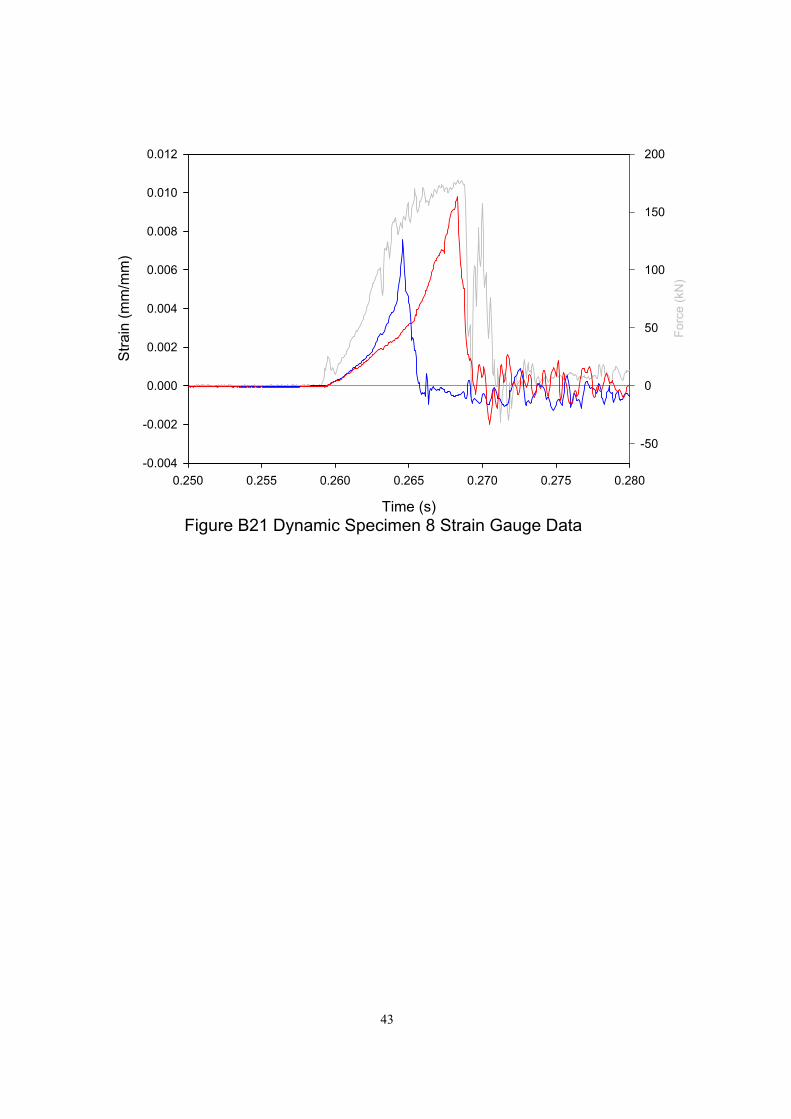
Figure B21 Dynamic Specimen 8 Strain Gauge DataTime (s)
0.250 0.255 0.260 0.265 0.270 0.275 0.280
Fo
rce
(kN
)
-50
0
50
100
150
200
Str
ain
(m
m/m
m)
-0.004
-0.002
0.000
0.002
0.004
0.006
0.008
0.010
0.012
43