Embed Size (px)
Citation preview

AUTONOMOUS SLAM ROBOT
Group 1 Project Report
PROJECT IN MECHATRONICS ENGINEERING
Lecturer: Peter Xu
Tutor: James Kutia
Department of Mechanical Engineering
University of Auckland
30 May 2015

iii
Abstract
In robotics, Simultaneous Localization & Mapping (SLAM) is the problem of constructing a map
of an unknown environment while also keeping track of the location of the robot within that
environment. This project entails the utilization SLAM techniques to develop an autonomous
vacuum cleaning robot.
A combination of three IR sensors, a servo, and a 9DOF Motion processing unit were
implemented alongside an Arduino Mega 2560 on a Vex robotics mecanum robot to provide the
desired functionality. A spiral path was used, with the robot travelling around the exterior of the
environment, before incrementing its distance from the boundary on each successive lap.
Readings from each of the sensors were fused to provide a robust estimation of the robots
trajectory, while simultaneously monitoring its path for objects and providing course adjustments
to avoid collision.
Sensor data was transmitted wirelessly via Bluetooth and displayed via a LabVIEW user
interface, and continuously updated in real time with the robots path, current position, and the
location of any obstacles.

iv

v
Table of Contents
Abstract ..................................................................................................................................... iii
Table of Contents ........................................................................................................................ v
Table of Figures ........................................................................................................................ vii
Table of Tables ......................................................................................................................... vii
Glossary / Abbreviations ........................................................................................................... vii
2 Introduction ......................................................................................................................... 1
3 Problem Specifications ........................................................................................................ 1
4 Mechanical Design .............................................................................................................. 2
4.1 Provided Hardware ....................................................................................................... 2
5 Hardware Configuration ...................................................................................................... 3
5.1 Iteration 1 ..................................................................................................................... 3
5.2 Iteration 2 ..................................................................................................................... 3
6 Low Level Functions ........................................................................................................... 5
6.1 Motor Operations .......................................................................................................... 5
6.2 Orientation Operations .................................................................................................. 6
6.2.1 MPU ...................................................................................................................... 6
6.2.2 Yaw Correction ..................................................................................................... 7
6.2.3 Robot Orientation .................................................................................................. 7
6.3 IR Sensor Operations .................................................................................................... 7
7 User Interface & Communications....................................................................................... 8
7.1 Communications ........................................................................................................... 8
7.2 LabVIEW Program ....................................................................................................... 8
7.3 LabVIEW Features ....................................................................................................... 9
8 Path Design ........................................................................................................................ 10
8.1 Bouncing .................................................................................................................... 10
8.2 Zig-zag ....................................................................................................................... 11
8.3 Spiral .......................................................................................................................... 12
9 Obstacle Avoidance........................................................................................................... 12
9.1 Detection .................................................................................................................... 12

vi
9.2 Avoidance................................................................................................................... 13
9.3 Walls .......................................................................................................................... 13
10 Localisation ....................................................................................................................... 13
10.1 Initialisation ............................................................................................................ 14
10.1.1 Trialled Initialisation Methods ............................................................................. 14
10.1.2 Final Initialisation method ................................................................................... 15
10.2 Room Sizing ........................................................................................................... 16
10.3 Co-Ordinate System ................................................................................................ 16
10.4 Sensor Fusion .......................................................................................................... 17
10.5 Wall Following ....................................................................................................... 17
11 Mapping ............................................................................................................................ 17
12 Testing & Results .............................................................................................................. 18
12.1 Testing Procedures .................................................................................................. 18
12.2 Results .................................................................................................................... 18
13 Conclusions ....................................................................................................................... 19
14 References........................................................................................................................... 1
Appendix A ........................................................................................................................... 13-1
Appendix B ............................................................................................................................ 13-4

vii
Table of Figures
Figure 1: Servo actuated turret assembly ..................................................................................... 3
Figure 2: Final Hardware Arrangement ....................................................................................... 4
Figure 3: Hardware Connections ................................................................................................. 5
Figure 4: The LabVIEW user interface ........................................................................................ 9
Figure 5: Bouncing Path Example ............................................................................................. 10
Figure 6: Zig-zag Path Example ................................................................................................ 11
Figure 7: Spiral Path Example ................................................................................................... 12
Figure 8: Initialisation Scan ...................................................................................................... 14
Figure 9: Example Range Data .................................................................................................. 15
Figure 10: Wall Alignment........................................................................................................ 16
Figure 11: Co-ordinate system calculation ................................................................................. 17
Figure 12: Comparison of robot mapping (left) vs. actual path (right) ....................................... 18
Figure 13: Final Demonstration Actual Path .............................................................................. 19
Table of Tables
Table 1: Arduino Pin Connections............................................................................................... 5
Table 2: Gyroscope & Accelerometer Offsets ............................................................................. 7
Table 3: Commands in the LabVIEW program ........................................................................... 9
Glossary / Abbreviations
FIFO First In, First Out
IR Infrared
Strafe / Strafing Sideways movement

1
1 Introduction
In robotics, Simultaneous Localization & Mapping (SLAM) is the problem of constructing a map
of an unknown environment whilst also keeping track of the location of the robot within that
environment. This is a difficult problem, as the quality of the map is dependent upon the
accuracy of the robot’s location. However, locating the position of the robot usually relies on
accurate mapping.
The aim of this project is to develop an autonomous vacuum cleaning robot using SLAM
techniques that will provide complete coverage of a room whilst avoiding any obstacles
encountered during the process. It should cover the floor area of the room in the fastest possible
way and also build a map of its path, the boundary of the room, and the location of any obstacles
encountered as verification of complete room coverage.
2 Problem Specifications
The key requirements of the project are as follows:
Autonomous – The robot must run on its own, without human intervention, once
it has begun its vacuuming routine.
Obstacle Avoidance – The robot must be able to navigate around randomly
placed objects in the room. Collision with any obstacles, or the walls of the room,
is not permitted.
Mapping – The robot must record a map of the path in which it has travelled
while vacuuming the room.
Completion Time – Robot should use the fastest path.
Coverage – The entire floor area must be covered by the robot, except any that is
occupied by obstacles.
Hardware – The team must use only the provided key hardware components
(sensors/actuators).

2
3 Mechanical Design
3.1 Provided Hardware
Arduino Mega 2560 & Sensor Shield – Microcontroller development board based around
the ATmega2560, with 54 digital I/O pins, 16 analog inputs, a 16MHz clock speed and 8KB
of SRAM [1]. The sensor shield facilitates the integration of sensors and actuators by
allowing the Arduino regulator to be bypassed and full battery voltage delivered to digital
I/O pins 46-50. It also provides an individual +5V, ground and signal pin for all other I/O
pins which simplifies wiring.
SHARP YA021 & YA020 – Medium & Long range infrared sensors. These output an
analog voltage corresponding to the distance of the target. The analog voltage is read by the
Arduino ADC’s and converted to range in software, measured in cm. The medium range
sensor has an operational range from 10 to 80cm [2], while the long range sensor operates
from 20-150cm [3].
LV-MaxSonar –EZ20 – Ultrasonic Sonar sensor which provides range measurements via
serial, analog voltage, and a digital pulse width output. Has an operational range of 0 to 6.5m
[4]. However it suffers from significant noise and due to its nature, it is difficult to
determine what bearing the target lies on, only its range. Due to these limitations the sonar
sensor was omitted from the final design.
MPU-9150 - A motion processing unit consisting of a 3 axis MEMS gyroscope,
accelerometer and magnetometer and on-board processor. Communicates with the Arduino
via the I2C protocol and provides heading and acceleration information [5].
Servo – Generic (Sub Micro Size) – Small servo that operates on 5V and has a range of
zero to 160 degrees. Maximum speed at 5V is 600 degrees/sec, with a maximum torque of
0.14 Nm. Input is a pulse width value from a digital I/O pin on the Arduino [6]
Mecanum Robot – Based on Vex Robotics components, utilizes four full rotation servos to
drive four mecanum wheels, allowing for omnidirectional movement. Power Supply is a
7.4V (2S) 2200mAh Lithium Polymer battery [7].
3
4 Hardware Configuration
Figure 1: Servo actuated turret assembly
4.1 Iteration 1
Initially, the ultrasonic sensor was also mounted on a rotating turret along with the IR to take
advantage of its much greater range. However, the signal was noisy and considerably less
accurate than the IR and, due to the width of the beam it was very difficult determine the bearing
of the obstacle. The turret configuration also caused the sensors to translate which complicated
interpretation of the data from them. Another IR sensor was also mounted at the rear of the robot
but it was found to be redundant and removed for the final design.
4.2 Iteration 2
The final hardware configuration uses the MPU in addition to three of the IR sensors. The
Arduino and sensor shield are mounted at the rear of the robot, with the cluster of sensors
mounted on an ABS frame positioned at the robots centre. Mounting the sensors in the centre
served several purposes, one of which was minimising the impact of the IR sensor’s short range
dead bands. The medium range IR sensors cannot give valid readings at distances less than 10cm.
In order to reduce the impact this had on the system they are mounted in the centre of the robot so
that most of that 10cm lies within the bounds of the robot.
The center of the robot was chosen as the reference point, so situating all the sensors within a
close distance of this reduced the need to include offsets to provide accurate localisation.

4
Figure 2: Final Hardware Arrangement
1. Left IR Sensor (Medium Range) – Provides range data that is used determine the
distance the robot is from the wall, and for obstacle avoidance. Mounted in the center of
the robot so that the dead band of the sensor extends only slightly beyond robots frame.
2. Rotating IR Sensor (Long Range) – Sensor is rotated by servo from +80 to -80 degrees
to check the path of the robot for obstacles. Also used to determine the Y position of the
robot when the sensor is at its center position (0 degrees). Mounted in the center of the
robot to reduce the effect of the sensors dead band, with its axis coincident to the servo
output to prevent translation during servo operation.
3. Arduino Mega 2560 & Sensor Shield – These have been shifted backwards from the
stock configuration to prevent them from obscuring the view of the IR sensors and
allowing the servo to be mounted at the robot’s center.
4. Bluetooth Module – Used for serial communication and control of the robot through the
Putty terminal or LabVIEW program.
5. Right IR Sensor (Medium Range) Provides range data that is used to determine the
distance the robot is from the wall and for obstacle avoidance. Mounted in the center of
the robot so that the dead band of the sensor extends only slightly beyond robots frame. .
6. 9 Axis Motion Processing Unit (MPU9150) – Provides orientation data from the
gyroscope. Mounted behind the IR turret on the robot’s axis of rotation to ensure
accuracy. On a rubber isolator to reduce noise from robot operation.
7. Servo – Used to rotate the IR sensor.
1
4
3
5
2
6
7

5
Table 1: Arduino Pin Connections
Component Pin Number
Left IR Sensor Analog I/O 1
Right IR Sensor Analog I/O 2
Rotating IR Sensor Analog I/O 3
Rear IR Sensor Analog I/O 4
MPU9150 SDA/SCL
Bluetooth Module TX1/RX1
Sensor Servo Digital I/O 45
Wheel Servo 1 Digital I/O 46
Wheel Servo 2 Digital I/O 47
Wheel Servo 3 Digital I/O 48
Wheel Servo 4 Digital I/O 49
5 Low Level Functions
5.1 Motor Operations
The robot used 4 motors that were controlled via VEX Motor Controller 29s that take a PWM to
set the motor speed. The PWM used by the motor controllers follows the servo PWM protocol in
which a pulse width of 1500μs is zero speed or neutral. A pulse width greater than 1500μs would
result in forwards rotation, while a pulse width less than 1500μs results in a reverse rotation.
Due to the nature of the mecanum wheels used on the robots, the motion of the robot could be
broken into three components, forwards speed, strafing speed and rotational speed. These 3
Figure 3: Hardware Connections
6
motion types could be combined to form a single required motion for each wheel that was then
sent to each wheels respective controller.
To decide how to combine each of the different desired motions into outputs for the wheels a
state machine for driving was made with states for forwards (FORWARDS), backwards
(BACKWARDS), left strafing (LEFT), right strafing (RIGHT), rotating on the spot (YAW) and
stopping (STOP). Depending on which drive state the robot was in the robot would combine
motion variables together differently. Appendix B 1 shows how the different drive types are
selected by the desired drive type.
When in the FORWARD state, the parts that make up the forward component of speed are purely
the set speed, the strafing motion (which is an input of the wall following controller to maintain a
fixed distance), and the rotational motion (which is set by the heading controller so that the robot
faces the target direction). However in a strafing mode such as LEFT, the forwards component is
set to zero with the set speed instead being used for the sideways motion. Rotational motion is
still set by the heading controller. When the drive state is set to YAW, both forwards and
sideways motion are set to zero, and the only motion is set by the heading controller.
These drive states are set depending on the part of the path the robot is in. For example when
following a wall, the drive state will be FORWARD. When an obstacle appears the drive state
will be set to LEFT or RIGHT by the collision avoidance controller. When the robot reaches a
corner the drive state will be set to YAW.
The separation of motion into 3 components allows for odometry to be used for localization
purposes. The amount travelled forward per cycle can be calculated as a function of the forward
component of the speed very reliably, just as the sideways travel component can be used to
determine how far the robot has travelled sideways.
5.2 Orientation Operations
A MPU-9150 motion processing unit was used to determine the robots orientation. The main
parameter of interest was the Yaw position of the robot. Using the built in DMP (Digital Motion
Processing) unit on the MPU, the yaw, pitch, roll angles of the robot are made available. The
orientation was then used by multiple functions on the robot including: driving straight (yaw
correction), setting travel direction, and mapping.
5.2.1 MPU
By using the integrated DMP on the MPU the processing power required by the host
microcontroller is greatly reduced. The MPU provided was the 9-axis MPU-9150. However after
experimenting with various setups it was decided that only 6-axis (accelerometer and gyroscope)
were needed. This meant the chip could have been replaced with the cheaper MPU-6150 if
money needed to be saved. The MPU handles the sensor fusion of gyroscope and accelerometer
values to calculate the required orientation angles. The update rate of the MPU was reduced to
50Hz to improve stability after there were stability issues when operating at the default 100Hz.

7
On initial start up the MPU requires the robot to be stationary in order to stabilise the output, the
time required for this was greatly improved by calibrating the offset values for both the
accelerometer and gyroscope, and these are shown in Table 2.
Table 2: Gyroscope & Accelerometer Offsets
Offset Value
X Gyroscope 212
Y Gyroscope 68
Z Gyroscope 46
X Accelerometer 86
Y Accelerometer 23
Z Accelerometer 1652
5.2.2 Yaw Correction
Due to the nature of the servo motors being used there was some variation in the speeds of each
motor at different loadings. This combined with potential slippage against the floor caused
significant deviation when the robot tried to drive straight. By setting a target yaw position, and
implementing a controller to maintain this position the robot was able to drive relatively straight.
The control was originally intended to be implemented using a PID controller. However upon
testing it was found that a standard P (proportional) controller was adequate and performed to the
requirements without the added complexity of a full PID controller. During testing it was found
that a gain of 12 provided good performance. A clamp was also implemented to avoid an invalid
output to the motors, this clamp value was set to ±300.
5.2.3 Robot Orientation
Because the robot is able to rotate as well as move in a 2D manner, a fixed orientation frame
needed to be created. Upon initialization the robots orientation was zeroed parallel to the first
wall it found. Any orientation position from that point on would be with respect to this frame. To
make things more simple it was decided that the robot would only travel aligned to either the X
or Y axes. This meant that the orientation could always be described as north, south, east, west or
transitioning. A global variable was used to store the current orientation to make future cases
easier to deal with.
5.3 IR Sensor Operations
A simple moving average filter was implemented on the output from the IR sensors. The latest 5
values received at 20 Hz were averaged to provide a smoother output. This filter was used for
both the left and right sensors at all times, but for the front long range sensor it is only used when
it was facing directly forwards (servo at 0°).
Two medium range (10-80cm) IR sensors were selected to face sideways on the robot with one
long range (20-150cm) mounted on the turret. The medium ranged IRs were chosen to give

8
greater accuracy for the robot to follow walls, and with the long range sensor being used to get a
more complete picture of the entire room.
The conversion from the voltage output to range was taken directly from the data sheet of the
sensors and no extra calibration was used. This meant that if one of the sensors failed, another
one could be put in place without having to recalibrate the conversion. This did mean that more
conservative distances had to be taken for avoidance occasionally.
6 User Interface & Communications
The control and monitoring of the robot was performed wirelessly across a Bluetooth connection.
The communication was used to monitor and perform additional controls of the robot, however
the robot is completely independent and does not rely on any commands from the user.
6.1 Communications
The Bluetooth communication is performed using the supplied Bluetooth module for Arduino.
This module allows for wireless serial communication between the robot and a client computer.
The communication is based on a Client-Server setup where the robot acts as the server and the
remote computer is the Client. This form of communication means that the server is not
continuously outputting data when there are no client connections, therefore it is not wasting
resources on the robot. Instead the program waits for the computer program to send a
request/command to the robot. This command is then read and subsequent actions and a response
is given.
6.2 LabVIEW Program
The main interface was developed in the LabVIEW environment. Using the NI-VISA controls, a
serial communications link with the robot was established. In order to reduce the data loss and to
avoid overflowing, a queue system was used. The queue stores all application requests and
executes them on a FIFO basis. The next command is only sent when the previous command has
been completed, i.e. a response has been received.
The primary use of the interface was to achieve a level of control and receive basic information
about what the robot is doing. Commands were setup to drive the robot using the four arrow keys.
In the earlier stages of development sensor data and program variables were able to be
synchronously displayed on the LabVIEW program in real-time allowing for much easier
debugging and fault identification. Charts and XY plots made data interpretation very user
friendly resulting in faster development of the program.

9
Figure 4: The LabVIEW user interface
6.3 LabVIEW Features
Figure 4 shows the LabVIEW user interface. The interface consists of:
(a) The Room Map – This shows the robot’s current position (purple square), as well as past
positions (white dots), and observations (green dots).
(b) IR Sensor Data – This shows the data from the IR sensors in a visual display. The dots on
the front, left, right, and back show obstacles in the respective directions (The rear IR was
later decided to be unnecessary and omitted).
(c) History Charts – The charts show historic data from the robot, and these can be overlaid to
make comparison easier.
(d) Localisation Information – These values give information on the position of the robot as
well as how far through the sweep it is.
(e) Status Information – This gives an indication on the current status of the robot including
what modes are active and the current battery level.
(f) Orientation Display – This shows the current orientation of the robot (yaw angle).
The main method of controlling the robot was done using keys on the keyboard. Table 3 shows a
list of commands used in the demonstration version of the program. Additional commands and
displays were created during testing to display variables (such as collision, walls, IR distances)
that were omitted from the final version.
Table 3: Commands in the LabVIEW program
Command Action Response
←, ↑, →, ↓ Change Robot Direction Current Direction
‘A’ or ‘a’ Reduce Yaw Target by 90° Current Yaw Target
‘D’ or ‘d’ Increase Yaw Target by 90° Current Yaw Target
‘C’ or ‘c’ Toggle Collision Detection Current Collision Detect State

10
‘I’ Start Initialisation “Starting Initialisation”
‘i’ Get Sensor Data “S[IR_R],[IR_B],[IR_L],[IR_B]”
‘P’ or ‘p’ Get Position Data “P[shortDist],[longDist],[Yaw]”
‘G’ or ‘g’ Toggle Gyro Correction Gyro Correction State
‘Z’ or ‘z’ Zero Gyro & Odometry “Gyro Zero’d”
‘W’ or ‘w’ Toggle Wall Follow Wall Follow State
‘[‘ Reduce Target Wall Dist Current Wall Distance
‘]‘ Increase Target Wall Dist Current Wall Distance
‘M’ or ‘m’ Toggle Spiral Control Current Spiral State
‘<’ Decrease Speed Current Speed
‘>’ Increase Speed Current Speed
‘Y’ or ‘y’ Set Drive State to YAW “Yaw”
‘u’ Get Current Status “U[ControlStates],[Battery],
[WallDist],[TotalX],[TotalY]”
7 Path Design
Several different path designs were trialled during this design project. A simple path design that
could have been used was a bouncing path; that is similar to what the commercial equivalent
Roombas already use [8]. A bouncing path is a simple path in which the robot drives forwards
until it encounters something it cannot pass at which point it turns so as not to hit the object then
continues on forwards. Another major path design was a zig-zag path in which the robot would
always travel parallel to one wall, increasing its distance from the wall as it reached the ends of
the room. The last path design (that was eventually used in the final iteration of design) was a
spiral that travelled a set distance from a wall until it reached another wall, at which point it
would travel the same distance from that wall.
7.1 Bouncing
Figure 5: Bouncing Path Example
A bouncing path would have been very easy to implement initially. Using our obstacle avoidance
protocols, the response to every obstacle could have been set to be a fixed angle turn to avoid the

11
obstacle, after which the robot could drive straight again. This path has the benefit of being
computationally cheap requiring very little higher level control. However, there are some costs.
One of the most obvious negative factors is that coverage is not guaranteed. Depending on the
arrangement of the room, large portions of the room could be untouched as the robots bouncing
angles will not allow it to reach certain area, or it could easily be trapped within a space of
objects. The other issue with such a design is that the robot could take a longer time to reach
similar coverage levels than other paths. This is caused by the robot going over areas several
times as it bounces around. Another issue that arises from this path is knowing when the robot is
complete, although this could be solved by having a fixed time for running at which point the
robot stops regardless of coverage or position.
7.2 Zig-zag
Figure 6: Zig-zag Path Example
The first path that was developed to be tested was a zig-zag path. To use this path the robot has to
travel at a set offset from a particular wall. This offset is increased once the robot reaches the end
of the wall, and the robot turns around. This travel path would allow for very good coverage as
the offset increments could be set so that the robots forwards and return paths were 1 body width
different allowing for maximum coverage with minimal overlap resulting in a good time to
completely cover a space. One key limitation of this path is that with the hardware set-up used, it
was critical that the robot finds a short wall and aligns itself well to this wall. This is so the robot
can have vision of at least one wall on its side as it travels along the long walls. This set up also
relies on an accurate coordinate system to handle the robot’s path when doing the second part of
the map, as it can no longer see the original reference wall.

12
7.3 Spiral
Figure 7: Spiral Path Example
The final path used was a spiral pattern. The robot will drive forwards and initialise. After the
robot has found a wall it will drive at a set offset until it reaches another wall, where it will rotate
90° and drive along the new wall. Once the robot has completed a full lap (indicated by it facing
the same direction as it started) it will increase how far from the wall it follows. The spiral path is
similar to the zig-zag path in that it follows a wall at a set offset, but for a spiral the wall that is
followed is always on the left (to perform a clockwise spiral) thus removing the need to merge
the readings from the two side sensors as required to take a zig-zag path. This path has many
advantages that led to it being selected as the final path to be implemented. One of the key
advantages is that it can begin on any wall which was one of the limitations of the zig-zag path. It
still has good coverage without large overlap and good time. The robot can also know when it is
done covering the room because the offset will be larger than half the size of the room and it will
stop (or in a real world application return to its dock).
8 Obstacle Avoidance
Obstacle avoidance can be broken down into two steps. First the robot has to detect the collision,
after which it must decide what action should be taken to avoid the collision.
8.1 Detection
The first step in avoiding an obstacle is to detect its presence. For the purpose of this project an
object was anything that is in the path of the robot less than 24cm in the forwards direction. An
object that is less that 24cm from the centre of the robot in the forward direction and within 14cm
on the left and 16cm on the right is an obstacle that must be avoided. The reason for the
asymmetrical collision box was to allow the robot to get closer to the wall (and achieve coverage
near the wall). Appendix B 6 shows how the detection of objects in handled.
To detect where an obstacle is within this collision zone the long range IR sensor mounted on the
servo motor sweeps a 90° cone centred around the central axis of the robot using 5 angles evenly
spread across the cone. The code for this scan is shown in Appendix B 7. The range data read is

13
then converted from polar to Cartesian coordinates. If any of the measured points is within the
collision zone the robot go into the collision avoidance controller which will decide the best
action to take to avoid the object.
8.2 Avoidance
Once the robot has determined that a collision is likely it will enter into its collision avoidance
programming. A section of the code that handles avoidance is shown in Appendix B 5. There are
several steps to the avoidance that take place. The first step the robot takes is to stop and gain a
better picture of the situation it is in. To insure that it has accurate information about the obstacle
it will run a full scan while stationary. Once a full scan has been completed the robot will
determine which side is the best to try going around the object in the first instance. The best side
is determined by calculating the strafing direction that would require the shortest amount of travel
to avoid the obstacle. If the object is mostly on the left hand side of the robots central axis the
shortest path initially tried will be to go to the right.
Once the robot has determined the best direction to try strafing first. It will strafe until the object
is no longer in the collision zone. If the robot determines that the direction it is trying to travel is
blocked using the IR sensors facing sideward, it will try the other direction ie if the robot was
strafing right and there is an obstacle on the right side, the robot will go left.
Once the robot has strafed enough to avoid the obstacle it will travel forward until it has passed
the object at which point it will strafe back. Once the robot has strafed back it will continue on
the spiral path.
8.3 Walls
Another situation that is partially handled by the collision avoidance protocols is wall detection.
The detection of walls is used to give the spiral path following control, the information required
to turn a corner. The robot defines a wall as an object that is seen in all 5 positions near the robot.
For wall detection a fixed distance is used rather than a Cartesian conversion. When a wall is
seen in front of the robot the spiral path controller is informed and will update the path.
9 Localisation
For localization both sensor readings and odometry of the robot are used. The left IR sensor and
odometry are used to provide the distance from the left wall, odometry is used exclusively when
an obstacle is between the IR sensor and the wall. Distance from the rear wall is predominantly
determined using odometry, as this was found to provide reasonable accuracy. The robots yaw
angle is determined using the output from the gyroscope, this proved to be quite accurate, with
minimal drift during test runs (as long as the gyroscope was provided with enough time to settle,
whilst the robot is stationary).

14
9.1 Initialisation
When the robot is first started up it needs to initialize, find a wall and determine its orientation.
There were several methods of initialization that were created and tested. Initialisation was
divided into two main parts, finding a wall and aligning to the wall.
9.1.1 Trialled Initialisation Methods
One of the methods that was trialled for initialization was scanning the whole room to find a wall
then aligning to it. To scan the whole room the robot did a higher resolution scan than normal
with the long range sensor covering a larger field of vision with more steps per degrees. It would
then turn 90° and do another scan, repeating until it had scanned 360°. The scan cone was set so
that there would be overlap between 2 adjacent scans as shown in Figure 8.
Figure 8: Initialisation Scan
An example of the range data gathered by the robot and post processed for display purposes is
shown in Figure 9. From this scan data there were several methods to find walls that were
investigated including a line finding algorithm and a largest distance method. A line finding
algorithm would compare groups of data points to work out the probability that the points lie on
the same straight line. Lines that had substantial length could be interpreted as walls, and the
robot could then head towards one of the lines it found.
The largest distance method looked at two data points from scans that were 180° apart that could
then be paired. In Figure 8 examples of points that would be paired are 1A would be paired with
3A, and 2A paired with 4A. The largest pair would indicate something that the robot would be
able to align to, so the robot would drive towards it and complete its initialization there.

15
Figure 9: Example Range Data
9.1.2 Final Initialisation method
During initialisation the robots starts by driving forward until it sees an object within 40cm of it.
The robot will then try to align to the object using 3 scan points at -30°, 0° and +30°. After
getting range information from these 3 points, it will try to make the 2 outer measurements equal
by rotating a calculated amount as shown in Figure 10. The middle distance is used to help
determine cases such as the robot facing into a corner or trying to orient to an obstacle. In these
cases the robot would be able to have both outer ranges equal while not being perpendicular to a
wall. The robot will perform an alignment calculation 3 times. It will then check to see if has
successfully aligned to the wall. If it has not aligned, it will turn 90° and drive straight until it
finds another object it can try align to. The initialisation process will repeat until the robot has
successfully aligned to a wall, at which point the offset for the orientation and position can be set
and the robot can begin processing the room as shown in slide 4 of Figure 10.
0
20
40
60
80
100
120
140
160

16
Figure 10: Wall Alignment
9.2 Room Sizing
During the first loop of the room the robot calculates the size of the room. This is achieved by
measuring the total forwards movement (using odometry) on each side of the room. This
movement is then added to the wall offset at each end to give the total length of the wall. Once
these values are calculated the position of the robot can be calculated based on the distance from
two walls.
9.3 Co-Ordinate System
Due to the specification that the room will always be rectangular, the current position of the robot
can be represented in terms of three parameters, the distance from the robot’s left & back wall, as
well as the robots current orientation. Once the room size is known (after the first loop) these
three parameters can be used to give a global XY co-ordinate. For the example shown in Figure
11, the distance from the orientation is south, the left wall distance is d1 and the back wall
distance is d2. The X co-ordinate is equal to the difference of Xtotal and d1, while the Y co-
ordinate is equal to the difference of Ytotal and d2. This position can then be used to start building
a map of the room and its contents.

17
Figure 11: Co-ordinate system calculation
9.4 Sensor Fusion
During testing it was found that using odometry alone for the current wall distance lacked the
desired accuracy. In order to achieve a more accurate wall distance the left IR sensor was used as
the primary measure, complimented with the odometry based on the motor outputs. The
weighting for the IR and odometry varies based on the current situation. For example, the IR
sensors cannot read a valid wall distance when there is an obstacle between the robot and the
wall. When this occurs the robots wall distance is weighted entirely on the odometry until the IR
sensor returns to a valid reading.
9.5 Wall Following
The wall following function maintains the robot at a set distance from the wall. This is essential
for the spiral path that was chosen. The wall following function employs a controller that adjusts
the strafing speed based on the error between the target wall distance and the actual wall distance.
The controller used was a P (proportional) controller, this provided adequate control without the
need of implementing a more sophisticated and resource heavy PID controller. The gain used was
found experimentally to be 10.
10 Mapping
Mapping is performed throughout the entire operation of the robot. Using the localization data
and the readings from the IR sensors a map can be generated. When the IR sensors are detecting
an object within their range this position is registered as a point of interest (POI) on the map. As
the robot moves around these POIs accumulate creating outlines of walls and obstacles in the
arena. This output can be viewed on the LabView UI program. Figure 12 shows a comparison of

18
the actual room layout and the map generated by the robot. The white dots represent the position
of the robot, while the green dots show observations (i.e. the detected objects / walls).
Figure 12: Comparison of robot mapping (left) vs. actual path (right)
11 Testing & Results
11.1 Testing Procedures
In order to test the robot a number of different courses were set up. This included various starting
positions and obstacle placements. These were all documented and improvements were made
when necessary. Due to time constraints, the desired amount of testing was not achieved.
However enough testing was completed to develop a solution that worked to an acceptable
standard in most applications.
11.2 Results
The robot performed exceptionally well during the demonstration runs. There were a couple of
small obstacle collisions that could have been avoided. If there was more time available collision
detection during strafing movements could have been implemented, avoiding these collisions.
The coverage of the robot was extremely good (Figure 13). There was very little overlapping
sections which resulted in an efficient path. The time taken to complete the course was very low,
which was another great achievement.

19
Figure 13: Final Demonstration Actual Path
12 Conclusions
The robot was completed, and its performance was to the standard given in the brief. Although
there were a few small mishaps the overall performance of the robot was great. The following
conclusions can be drawn from the project:
The robot performed the room sweep completely autonomously and did not require any
external intervention.
On the whole the robot was able to identify and successfully avoid most objects.
There is one case involving objects beside the robot and a strafing movement that could
be easily resolved in a future revision
The robot produced a map that showed similar resemblance to the actual map used during
the demonstration.
The time taken to complete the sweep was very quick and.
Coverage by the robot was very efficient, covering most of the arena with minimal
overlap.
The hardware used in the project was minimised which meant that the sonar sensor and
one IR sensor were not required in the final design.

1
13 References
[1] Arduino, "Arduino Board Mega 2560," [Online]. Available:
http://www.arduino.cc/en/Main/ArduinoBoardMega2560. [Accessed 05 May 2015].
[2] SHARP, "GP2Y0A21YK Datasheet," 2005. [Online]. Available:
http://www.sharpsma.com/. [Accessed 28 April 2015].
[3] SHARP, "GP2Y0A02 Datasheet," 2005. [Online]. Available: http://www.sharpsme.com/.
[Accessed 28 April 2015].
[4] MaxBotix, "LV-MaxSonar - EZ0 Datasheet," 2005. [Online]. Available:
www.maxbotix.com. [Accessed 28 April 2015].
[5] InvenSense, "MPU-9150 Datasheet," 05 May 2012. [Online]. Available:
http://www.invensense.com/. [Accessed 28 April 2015].
[6] Sparkfun, "Servo Generic sub-micro size," June 2013. [Online]. Available:
http://cdn.sparkfun.com/datasheets/Robotics/Small%20Servo%20-%20ROB-09065.pdf.
[Accessed 5 May 2015].
[7] "UnionBattery 2000mAh Specification," 16 March 2006. [Online]. Available:
https://www.sparkfun.com. [Accessed 28 April 2015].
[8] J. Layton, "How Robotic Vacuums Work," 03 November 2005. [Online]. Available:
http://electronics.howstuffworks.com/gadgets/home/robotic-vacuum.htm. [Accessed 01 May
2015].
[9] N. Wilkins, "Hardware Connections between Arduino and," 05 April 2013. [Online].
Available:
http://www.egr.msu.edu/classes/ece480/capstone/spring13/group08/documents/nori.pdf.
[Accessed 28 April 2015].
[10] MaxBotix, "MB1000 LV-MaxSonar-EZ20," [Online]. Available:
http://www.maxbotix.com/documents/MB1000_Datasheet.pdf.

2

A-13-1
Appendix A
Appendix A 1: Bill of Materials
Part Name Quantity Source
Mecanum Robot Kit 1 Lab stock
Arduino Mega 2560 1 Lab Stock
Sensor Shield 1 Lab Stock
MPU-9150 9DOF IMU 1 Lab stock
SHARP YA021 IR Sensor 2 Lab stock
SHARP YA020 IR Sensor 2 Lab stock
Bluetooth Module 1 Lab stock
Bluetooth Dongle 1 Lab Stock
Servo 9g (160 degree) 1 Lab stock
Vex Robotics Framing 1 Lab stock
Servo/IR sensor mount 1 Manufactured (3D Printed)
Rotating IR sensor mount 1 Manufactured (3D Printed)
M4 x 6 bolt/nut 6 Lab Stock
M3 x 16 bolt/nut 6 Lab Stock
Zip ties 5 Lab Stock

A-13-2
Appendix A 2: Mechanical Drawing of Turret Base
A-13-3
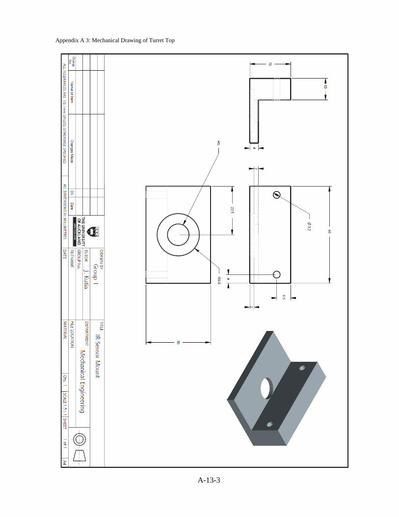
Appendix A 3: Mechanical Drawing of Turret Top

A-13-4
Appendix B
Appendix B 1: Drive Function
//Updates the motors to provide the desired type of motion
void DriveBetter()
{
switch (driveDirection) {
case STOP:
case WAIT:
Stop();
break;
case FORWARD:
Forward();
break;
case BACKWARD:
Backward();
break;
case LEFT:
Left();
break;
case RIGHT:
Right();
break;
case YAW:
Spin();
break;
}
UpdateDriveServos();
}
Appendix B 2: Forward Function
//Sets the 3 movement variables to generate forward motion with correction for
//heading and distance from the wall
void Forward()
{
ForwardSpeed = speed_val;
SpinSpeed = SpinPWM;
StrafeSpeed = WallCorrection;
}

A-13-5
Appendix B 3: UpdateDriveServos Function
//Combines the 3 movement variables in the required manner get
//achieve the required motion from each of the 4 wheels
void UpdateDriveServos()
{
int LF_Motor_pwm = - SpinSpeed - ForwardSpeed - StrafeSpeed;
int RF_Motor_pwm = - SpinSpeed - ForwardSpeed + StrafeSpeed;
int RR_Motor_pwm = - SpinSpeed + ForwardSpeed + StrafeSpeed;
int LR_Motor_pwm = - SpinSpeed + ForwardSpeed - StrafeSpeed;
left_font_motor.writeMicroseconds(1500 + LF_Motor_pwm);
left_rear_motor.writeMicroseconds(1500 + RF_Motor_pwm);
right_rear_motor.writeMicroseconds(1500 + RR_Motor_pwm);
right_font_motor.writeMicroseconds(1500 + LR_Motor_pwm);
}
Appendix B 4: WallFollow Function
//Determines error distance from target wall follow distance
//Sets a component of the wheels PWM output to correct for the error
void WallFollow()
{
WallCorrection = WallGain * -(wallTarget - actualWallDist);
//Limit the maximum and minimum values so as to not saturate the motors
if (WallCorrection > 150)
WallCorrection = 150;
else if (WallCorrection < -150)
WallCorrection = -150;
}
A-13-6
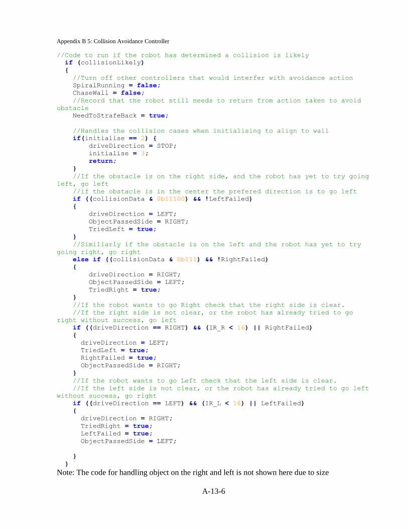
Appendix B 5: Collision Avoidance Controller
//Code to run if the robot has determined a collision is likely
if (collisionLikely)
{
//Turn off other controllers that would interfer with avoidance action
SpiralRunning = false;
ChaseWall = false;
//Record that the robot still needs to return from action taken to avoid
obstacle
NeedToStrafeBack = true;
//Handles the collision cases when initialising to align to wall
if(initialise == 2) {
driveDirection = STOP;
initialise = 3;
return;
}
//If the obstacle is on the right side, and the robot has yet to try going
left, go left
//if the obstacle is in the center the prefered direction is to go left
if ((collisionData & 0b11100) && !LeftFailed)
{
driveDirection = LEFT;
ObjectPassedSide = RIGHT;
TriedLeft = true;
}
//Similiarly if the obstacle is on the left and the robot has yet to try
going right, go right
else if ((collisionData & 0b111) && !RightFailed)
{
driveDirection = RIGHT;
ObjectPassedSide = LEFT;
TriedRight = true;
}
//If the robot wants to go Right check that the right side is clear.
//If the right side is not clear, or the robot has already tried to go
right without success, go left
if ((driveDirection == RIGHT) && (IR_R < 16) || RightFailed)
{
driveDirection = LEFT;
TriedLeft = true;
RightFailed = true;
ObjectPassedSide = RIGHT;
}
//If the robot wants to go Left check that the left side is clear.
//If the left side is not clear, or the robot has already tried to go left
without success, go right
if ((driveDirection == LEFT) && (IR_L < 16) || LeftFailed)
{
driveDirection = RIGHT;
TriedRight = true;
LeftFailed = true;
ObjectPassedSide = LEFT;
}
}
Note: The code for handling object on the right and left is not shown here due to size

A-13-7
Appendix B 6: CollisionDetection Function
//Based on mobile scan data determines if collision is likely
void CollisionDecection()
{
//Resets all collision data from previous run
collisionData = 0;
wallData = 0;
ObjectPosCount = 0;
TotalObjectCount = 0;
//Checks to make sure the rough scan is valid, and the robot is not
stopped
if (mobileScanValid && !(driveDirection == STOP))
{
collisionLikely = false;
//Checks through each of the scan positions
for (int i = 0; i < ROUGH_STEP_NUMBER; i++)
{
//Looks for walls in front of it
if (RoughY[i] < 40)
{
wallData += (1 << i);
}
//Looks for collisions
if (RoughY[i] < 24)
{
if ((RoughX[i] > -13) && (RoughX[i] < 16))\
{
collisionData += (1 << i);
collisionLikely = true;
//If a new collision is detected, the robot will force a
new scan to be taken, and wait until it is valid
if(newCollision)
{
mobileScanValid = false;
roughCheckIndex = 0;
newCollision = false;
}
}
}
}
}
}

A-13-8
Appendix B 7: MobileScan Function
//Sweeps using the servo and IR sensor.
void MobileScan()
{
//Only updates every 180ms to ensure good sensor values and not block
other functions
if (millis() - roughTimeStamp > 180)
{
roughTimeStamp = millis();
//Read the range data
Range = read_sharp_IR_sensor(SHARP_YA, A1);
//Convert polar co-ordinates to cartesian
servoAngle = M_PI * (-450 + roughCheckIndex * (900 /
(ROUGH_STEP_NUMBER - 1))) / (180 * 10);
RoughX[roughCheckIndex] = sin(servoAngle) * Range;
RoughY[roughCheckIndex] = cos(servoAngle) * Range;
roughCheckIndex = (roughCheckIndex + 1) % ROUGH_STEP_NUMBER;
//If a full scan has been done, indicate that the scan array has valid
data
if (roughCheckIndex == 0)
{
mobileScanValid = true;
}
//update servo position
Scanning_Servo.writeMicroseconds(TURRET_NEUTRAL - 450 +
roughCheckIndex * (900 / (ROUGH_STEP_NUMBER - 1)));
}
//Make sure that the servo angle is accurate for other functions
else if (millis() - roughTimeStamp > 50)
{
servoAngle = M_PI * (-450 + roughCheckIndex * (900 /
(ROUGH_STEP_NUMBER - 1))) / (180 * 10);
}
}


![AUTONOMOUS SIMULTANEOUS LOCALIZATION AND …homepages.engineering.auckland.ac.nz/~pxu012/mechatronics2015/group14.pdf · Beevers and Huang [2] utilise low cost IR sensors and a microcontroller](https://img.pdfslide.us/doc/110x75/5d478b2e88c993154f8b5af2/autonomous-simultaneous-localization-and-pxu012mechatronics2015group14pdf.jpg)