Project acronym: Project title: Grant agreement No · Authors Sveinn Agnarsson UIce 21/2/2018 SA ... D1.4, brings together all the methods used in PrimeFish and thus gives an overview

1

This project has received funding from

the European Union’s Horizon 2020

research and innovation program under

grant agreement No 635761

Deliverable No. 1.4

Project acronym:

PrimeFish

Project title:

“Developing Innovative Market Orientated Prediction Toolbox to Strengthen the

Economic Sustainability and Competitiveness of European Seafood on Local and Global

markets"

Grant agreement No: 635761

This project has received funding from European Union´s Horizon 2020 research and

innovation program.

Start date of project: 1st March 2015

Duration: 48 months

Due date of deliverable 28/02/2018

Submission date: 26/02/2018

File Name: PrimeFish_D1_4

Revision number: 01

Document status: Final1

Dissemination Level: PU2

1 Document will be a draft until it was approved by the coordinator 2 PU: Public, PP: Restricted to other programme participants (including the Commission Services), RE: Restricted to a group specified by the consortium (including the Commission Services), CO: Confidential, only for members of the consortium (including the Commission Services)

Ref. Ares(2018)1081005 - 26/02/2018

2





Revision Control

Role Name Organisation Date File suffix3

Authors Thong Tien Nguyen NTU 21/2/2018 TTN

Authors Nguyễn Ngọc Duy NTU 21/2/2018 NND

Authors Vo Van Dien NTU 21/2/2018 VVD

Authors Patrick Berg Sørdahl NOFIMA 21/2/2018 PBS

Authors Sveinn Agnarsson UIce 21/2/2018 SA

Authors Arnar Már Búason UIce 21/2/2018 AMB

Authors Antonella Carcagnì UPav 21/2/2018 BH

Authors Birgit Hagen UPav 21/2/2018 AC

Authors Stéphane Ganassali UNIV-SAVOIE 21/2/2018 SG

Authors Olga Untilov UNIV-SAVOIE 21/2/2018 OU

Authors louis-georges.soler@inra Inra 21/2/2018 LGS

Authors Irz Xavier Luke/Inra 21/2/2018 IX

Author Margrethe Aanesen UTro 21/2/2018 MAa

Author G.Kofi Vondolia UTro 21/2/2018 GKV

Authors Cristina Mora UNIPARMA 21/2/2018 CM

Authors Davide Menozzi UNIPARMA 21/2/2018 DM

Authors Marco Riani UNIPARMA 21/2/2018 MR

Authors Fabrizio Laurini UNIPARMA 21/2/2018 FL

Authors Giovanni Sogari UNIPARMA 21/2/2018 GS

Authors Gianluca Morelli UNIPARMA 21/2/2018 GM

Authors Katia Laura Sidali UNIPARMA 21/2/2018 KS

Data collection Heather Manuel MemU 21/2/2018 HM

Data collection Valur N.Gunnlaugsson MATIS 21/2/2018 VNG

WP leader Petter Olsen NOFIMA 26/2/2018 PO

Reviewer Valur N.Gunnlaugsson MATIS 26/2/2018 VNG

Coordinator Guðmundur Stefánsson MATIS 26/2/2018 GS

3 The initials of the revising individual in capital letters

3





Deliverable 1.4

PrimeDSF methods compendium, including sample data,

test runs, and comparative analysis

February 27th 2018

4





Executive Summary

The data used in the various tasks of PrimeFish comes from many sources. The approach taken

in the analysis within each task depends both on the objective of the task at hand, as well as the

data available. The methodology used in PrimeFish therefore spans a wide range of methods;

from quantitative and qualitative analysis of interview data and simple descriptive statistics to

state-of-the-art advanced statistical models.

This deliverable discusses the various methods used in the various tasks and deliverables.

Following a short introductory section, Sections 2-4 present the methodology used in work

package 2 (WP2). Section 2 presents the growth accounting used to assess productivity in the

harvesting sectors of Denmark, the Faroe Islands, Iceland, Newfoundland and Norway, while

Section 3 describes the data envelopment analysis to study efficiency and productivity in

aquaculture in several European countries and Vietnam. Section 4 presents the Kalman filter

method which is used to study the occurrence of boom-and-bust cycles in various seafood

markets. Section 5 discusses the method of co-integration which is used to analyse price

transmission and market integration. The global value chain analysis, upon which most of the

analysis in WP3 is based, in presented in Section 6 and Sections 7 and Section 8 present the

approach taken to study the how market institutions and labelling and certification affect

seafood and aquaculture firms. The analysis of European seafood products innovations is

discussed in Section 10, while the microeconomic models applied in WP4 are illustrated in

Sections 11 and 12. The methods chosen to analyse social awareness, attempts to stimulate fish

consumption, and negative press, are presented in Section 13. The choice experiments

conducted in WP4 are described in Section 14, while the fisheries and aquaculture

competitiveness index developed in WP5 is visited in Section 15. The methodology behind the

boom-and-bust model developed in WP5 is presented in Section 16 and the latent class analysis

and multinomial logistic regression used in WP5 is discussed in Section 17.

The wide variety of approaches shown in this deliverable show the breadth of the analysis

undertaken in PrimeFish, and the range of tools used to study the competitiveness of the

European seafood and aquaculture industries in this project.

5





Table of Contents

1 Introduction ......................................................................................................................... 6

2 Growth accounting .............................................................................................................. 7

3 Data envelopment analysis ............................................................................................... 12

4 Kalman filter ..................................................................................................................... 22

5 Price transmission and market integration ........................................................................ 28

6 Global value chain analysis .............................................................................................. 30

7 Value-chains: Market institutional analysis ...................................................................... 35

8 Value-chains: Labelling and certification ......................................................................... 36

9 Discrete choice analysis .................................................................................................... 39

10 Analysis of European seafood products innovations ........................................................ 44

11 Microeconomic demand analysis ...................................................................................... 45

12 Frequency of purchases ..................................................................................................... 57

13 Analysis of social awareness ............................................................................................ 63

14 Choice experiments ........................................................................................................... 64

15 Fisheries and aquaculture competitiveness index ............................................................. 69

16 Boom-and-bust model ....................................................................................................... 71

17 Latent class analysis and multinomial logistic regression ................................................ 73

References ................................................................................................................................ 89

6





1 Introduction

The overall objective of PrimeFish is to enhance the economic sustainability of European

fisheries and aquaculture sectors through new knowledge and insights about competitive

performance. The main aim of the project is to develop an innovative decision support

framework, PrimeDSF, which contains economic models and a decision support system,

PrimeDSS, that can be used by the industry and policymakers to better predict consequences

based on existing knowledge and simulation/forecasting models. The actual data collection and

analysis takes place in work packages (WP) 2-4, with the models making up the PrimeDSS

developed in WP 5.

WP1 is responsible for producing guidelines for consistent application of methods across the

project and also for collecting and collating usage reports from the different sectors, cases and

method users. The present deliverable, D1.4, brings together all the methods used in PrimeFish

and thus gives an overview of the different methodology applied in PrimeFish.

The data used in the various tasks comes from many sources. These include public national and

international agencies, sensitive firm-level data, interviews with business leaders and

consumers, consumer surveys and scanner-data on French consumers. The approach taken in

the analysis within each task depends both on the objective of the task at hand, as well as the

data available. The methodology used in PrimeFish therefore spans a wide range of methods;

from quantitative and qualitative analysis of interview data and simple descriptive statistics to

state-of-the-art advanced statistical models.

This deliverable discusses each of the different methods used. The methodology applied to the

different tasks is presented, sometimes in considerable detail, and where applicable the pros

and cons of using the approach chosen discussed. In some cases, examples are provided of the

data used, and the output obtained from using the models.

7





2 Growth accounting

Deliverable D2.2 analysed recent productivity developments in some of the most important

capture fisheries in Europe. The growth accounting representation chosen for this analysis was

introduced into the literature by Solow (1957) and later employed in empirical analysis of

productivity growth by several authors (Kendrick, 1961), (Jorgenson & Griliches, 1967) and

(Denison, 1972).

In the simple production process when one input is used to produce one output, output produced

per unit of input yields a comprehensive measure of productivity. However, matters become a

bit more complicated when several inputs are used to produce several outputs. Focusing on the

productivity on one input will then only yield partial productivity measures, such as for instance

output per worker per hour worked or output per unit of capital or machine hour. Although

commonly used, such measures provide an incomplete picture and may even “mislead and

misrepresent the performance of a firm” (Coelli, Rao, O’Donnell, & Battese, 2005, p. 62).

Labour productivity can, for instance, improve because of more skilled labour or because of the

additional usage of other inputs, such as capital.

To counter this, measures of multifactor or total factor productivity (MFP or TFP) have been

developed and applied to cases where a multitude of inputs are employed to produce several

outputs. By thus taking into account the changes that utilisation of all inputs has on production,

these measures provide a more accurate picture of productivity. Total factor productivity may

then be defined as the ratio of aggregate output produced relative to aggregate input used.

Following Arnason (2003) and Eggert and Tveterås (2013), the Törnqvist approximation of

total factor productivity change in fisheries in discrete time may be defined as

(1) 𝑇𝐹𝑃 = (𝑙𝑛 𝑌𝑡 − 𝑙𝑛 𝑌𝑡−1) − 𝛾𝛿1

2(𝑠𝑘𝑡 + 𝑠𝑘𝑡−1)(ln 𝐾𝑡 − 𝑙𝑛 𝐾𝑡−1)

−𝛾𝑡𝛿𝑡

1

2(𝑠𝑙𝑡 + 𝑠𝑙𝑡−1)(ln 𝐿𝑡 − 𝑙𝑛 𝐿𝑡−1) −

1

2(𝑠𝑎𝑡 + 𝑠𝑎𝑡−1)(ln 𝑆𝑡 − 𝑙𝑛 𝑆𝑡−1).

Here, Y represents landings which are measured in tons. Although fishermen may target one

specific species, there is also some bycatch of other species, which in many cases may be

considerable. In fisheries analysed in D2.2, Y is therefore always defined as aggregate of the

most important species targeted by fleet segment in question. In the case of demersal fisheries,

Y may therefore represent the combined catches of cod, haddock and saithe, and in the pelagic

cases Y may represent the combined catches of herring, mackerel and capelin. The precise

8





definition of Y does, however, differ between cases. K is defined as a capacity index that is

usually measured as the product of average vessel length, average engine size (in kW) and

number of vessels. This measure does therefore both take into account changes in the number

of vessels and harvesting capacity of the fleet. L is defined as the number of employed

fishermen or full-time equivalents. The value of the share of labour (sl) and capital (sk) in value-

added is taken from the economic accounts of the fishery. Finally, sa, represents the elasticity

of output with respect to stock, i.e. to the catchability of individual stocks which may differ

substantially between pelagic and demersal species, reflecting different distribution patterns of

stocks. Thus, while pelagic species tend to form schools, many demersal species tend to be

more evenly distributed. In the case of pelagic species the stock elasticity of output will

therefore take a value close to zero, indicating that even if stocks are large the schooling

behaviour of the specie in question may reduce its catchability, while in the case of demersal

species the elasticity may take a value close to unity. Empirical studies (Bjørndal, 1987;

Sandberg, 2006), have revealed a weak stock effect for pelagic species such as herring,

implying a value of close to zero for the stock elasticity, but a value close to unity for demersal

species (Hannesson, 1983; Hannesson, 2007a;Hannesson, 2007b; Sandberg, 2006).

As explained above, Y represents the total catches of the most important species of the relevant

fleet segment. In the Icelandic case, for instance, catches of cod, haddock, saithe, redfish,

wolffish and ling made on average up 89% of the total catches of the demersal fleet during the

period 2002-2014. If it can be assumed that harvesting of all species is equally capital- and

labour-intensive, which is a questionable assumption, it follows that capital and labour was only

utilised 89% of the time on the harvesting of these six species. In the productivity analysis, this

can be “corrected” by multiplying K and L by the parameter γ which takes on a value of unity

if Y includes catches of all the species harvested by the relevant fleet, but a value below unity

if catches of some species are excluded. In the Icelandic case, γ would therefore on average

take a value of 0.89.

In some of the cases included in D2.2, information exists on the number of days-at-sea, i.e. the

number of days spent searching for fishable quantities of the target species and time spent on

fishing. Where such information is available, it may be used to adjust the utilisation of capital

and labour, by multiplying K and L by the ratio of actual number of days-at-sea divided by 300,

i.e.

𝛿 =𝑛𝑢𝑚𝑏𝑒𝑟 𝑜𝑓 𝑑𝑎𝑦𝑠 𝑎𝑡 𝑠𝑒𝑎

300.

9





The denominator is set at 300 rather than 365 (the number of days in a year) to make allowance

for the fact that vessels may spend some day in harbour between fishing trips and to allow for

time for necessary refurbishment and maintenance. Both γ and 𝛿 will in general vary between

years, i.e. not take on fixed values.

Finally, in eq. (1) S represents an aggregate measure of the same stocks as included in Y. For

the Icelandic case, mentioned above, S would therefore be defined as the sum of the stocks of

cod, haddock, saithe, redfish, wolffish and ling. Stocks are usually defined as spawning stock

biomass (SSB) or fishable biomass if information on SSB is unavailable. The output elasticity,

sa, is set at 0.85 for all demersal species and 0.1 for all pelagic species.

Provided data are available on landings, capital, labour and stocks, as well as the share of capital

and labour, eq. (1) can then be used to calculate annual changes in total factor productivity for

the fishery in question. As stated in eq. (1), productivity growth will depend on changes in

landings, changes in the capital and labour, and changes in stocks. While increased landings

have a positive effect on productivity growth, decreased landings will retard productivity

growth. Increases in capital and labour will, ceteris paribus, decrease productivity growth, but

decreases in these control inputs will have a positive effect. It should be remembered that in the

studies included in D2.2, K is defined as a three dimensional capacity index that allows for

changes in the number of vessels, average length and average engine size. Thus, scrapping

programs that are aimed at reducing the number of vessels will encourage productivity growth.

However, the harvesting capacity of the vessels remaining in the fleet may increase enough to

compensate for the fall in vessel number. The end result could thus be an increase in K. In eq.

(1), stocks are treated just like a traditional input. Increases in stock size will then, ceteris

paribus, decrease productivity growth, while decreases in stocks enhance productivity growth.

In this analysis, fishing stocks is therefore considered a viable way to promote productivity.

This counterintuitive argument does though only hold in the short run, i.e. in the same year. In

the long-run fishing down stocks will decrease catches and may of course jeopardize the

existence of the fish species in question.

The growth accounting methodology was primarily chosen for two reasons. First, the models

can be applied in data-poor cases, i.e. when the data may only span a few years. Second, the

models are easy to implement, understand and interpret.

10





This methodology has though only been used relative infrequently. To date, there are only a

couple of other studies (Arnason, 2003; Eggert and Tveterås, 2013). Other studies are either

based on traditional micro economic models or DEA.

The main strength of this method is that it can be applied when there are relatively few data

points, much fewer than would be need for parametric or non-parametric analysis. The method

is also rather easy to implement and use, and interpret. The method is, however, based on rather

stringent assumptions, and cannot be used for out-of-sample predictions.

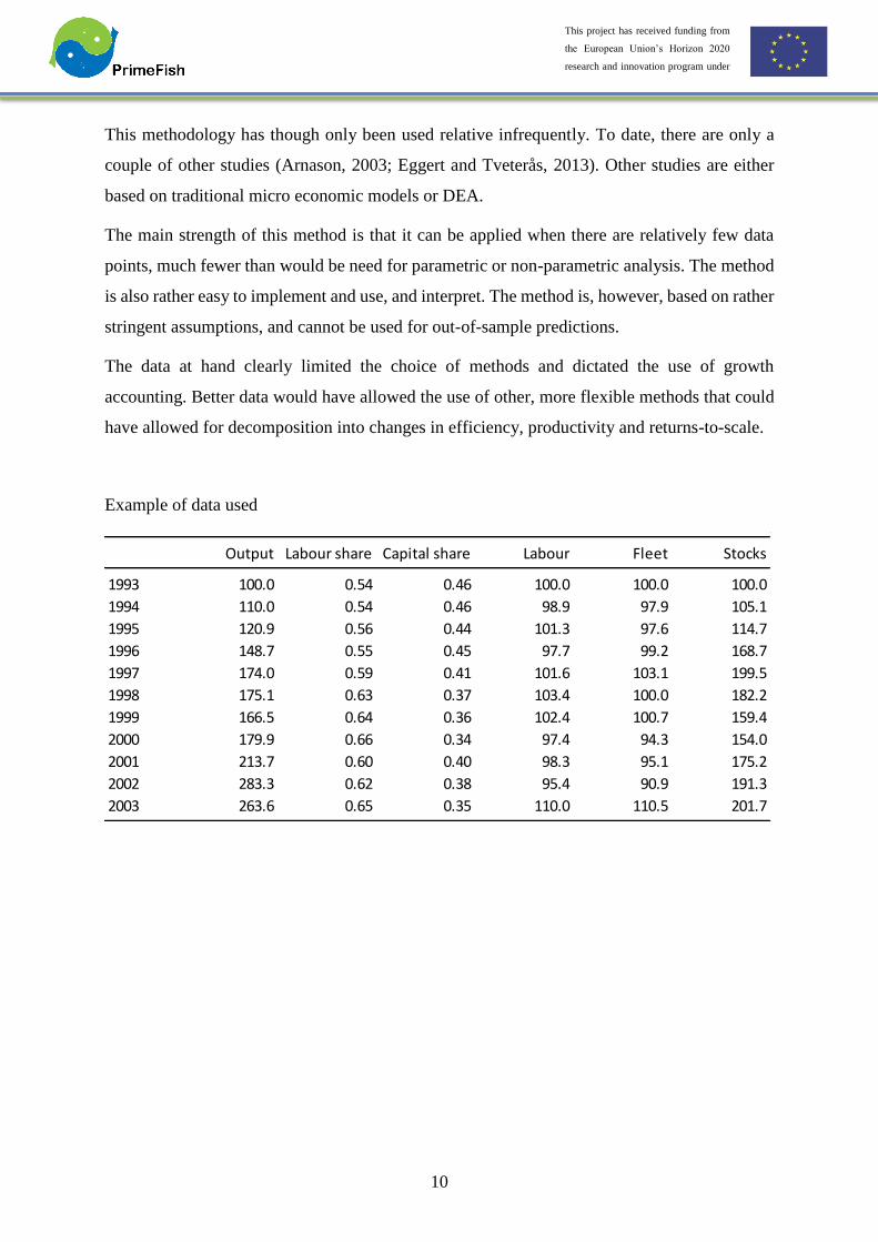
The data at hand clearly limited the choice of methods and dictated the use of growth

accounting. Better data would have allowed the use of other, more flexible methods that could

have allowed for decomposition into changes in efficiency, productivity and returns-to-scale.

Example of data used

Output Labour share Capital share Labour Fleet Stocks

1993 100.0 0.54 0.46 100.0 100.0 100.0

1994 110.0 0.54 0.46 98.9 97.9 105.1

1995 120.9 0.56 0.44 101.3 97.6 114.7

1996 148.7 0.55 0.45 97.7 99.2 168.7

1997 174.0 0.59 0.41 101.6 103.1 199.5

1998 175.1 0.63 0.37 103.4 100.0 182.2

1999 166.5 0.64 0.36 102.4 100.7 159.4

2000 179.9 0.66 0.34 97.4 94.3 154.0

2001 213.7 0.60 0.40 98.3 95.1 175.2

2002 283.3 0.62 0.38 95.4 90.9 191.3

2003 263.6 0.65 0.35 110.0 110.5 201.7

11





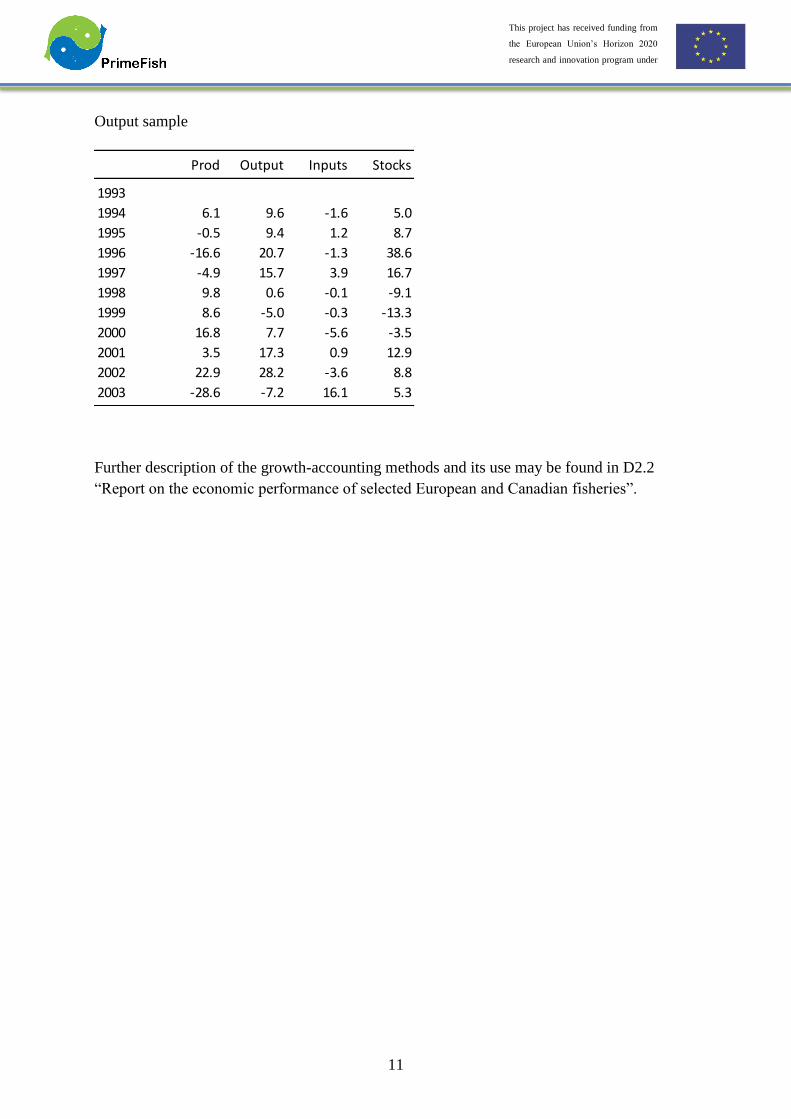
Output sample

Further description of the growth-accounting methods and its use may be found in D2.2

“Report on the economic performance of selected European and Canadian fisheries”.

Prod Output Inputs Stocks

1993

1994 6.1 9.6 -1.6 5.0

1995 -0.5 9.4 1.2 8.7

1996 -16.6 20.7 -1.3 38.6

1997 -4.9 15.7 3.9 16.7

1998 9.8 0.6 -0.1 -9.1

1999 8.6 -5.0 -0.3 -13.3

2000 16.8 7.7 -5.6 -3.5

2001 3.5 17.3 0.9 12.9

2002 22.9 28.2 -3.6 8.8

2003 -28.6 -7.2 16.1 5.3

12





3 Data envelopment analysis

Data envelopment analysis (DEA) was used in deliverable 2.3 (D2.3) in WP2. The objective of

D2.3 is to provide an overall picture of economic performance of aquaculture firm included in

some of the case studies in PrimeFish. In order to examine and understand the competitiveness

of key EU aquaculture industries, it was decided to compare the performance of two key fish

farming activities within the EU - Scottish salmon firms and Mediterranean sea bass and sea

bream firms – with two important international competitors – Norwegian salmon firms and

Vietnamese pangasius firms.

Economic performance may be defined in various ways, but it is most common to focus either

on financial indicators or productivity. D2.3 follows the latter approach and examine economic

performance using an advanced-methods named Data Envelope Analysis (DEA). DEA is a non-

parametric technique which allows productivity growth to be decomposed into changes in

efficiency and technology. Efficiency here refers to how well firms manage to utilise their

inputs to produce output, in this case farmed fish. Using DEA it is possible to construct an

efficiency frontier, which is made up of the most efficient firms, and calculate how far other

firms are from that frontier. The method also makes it possible to analyse shifts in the frontier,

which is taken to represent technical change. Firms can then either improve their productivity

by moving close to the efficiency frontier at each point in time, and/or take advantage of the

technical progress which shifts the frontier out. DEA also makes it possible to decompose

technical efficiency into pure technical efficiency and scale efficiency which measure how well

firms are able to utilise the scale economies available.

Technical efficiency is one component of overall economic efficiency, which is referred to as

the ability of a firm to obtain either maximal output from a given set of inputs (output-

orientation) or the optimal combination of inputs to achieve a given level of output (an input-

orientation), given the production technology (Coelli et al., 2005, p.51-56). Both input and

output measures can be used in order to compare technical efficiency between firms and over

time (Kumbhakar and Lovell, 2000, Coelli et al., 2005).

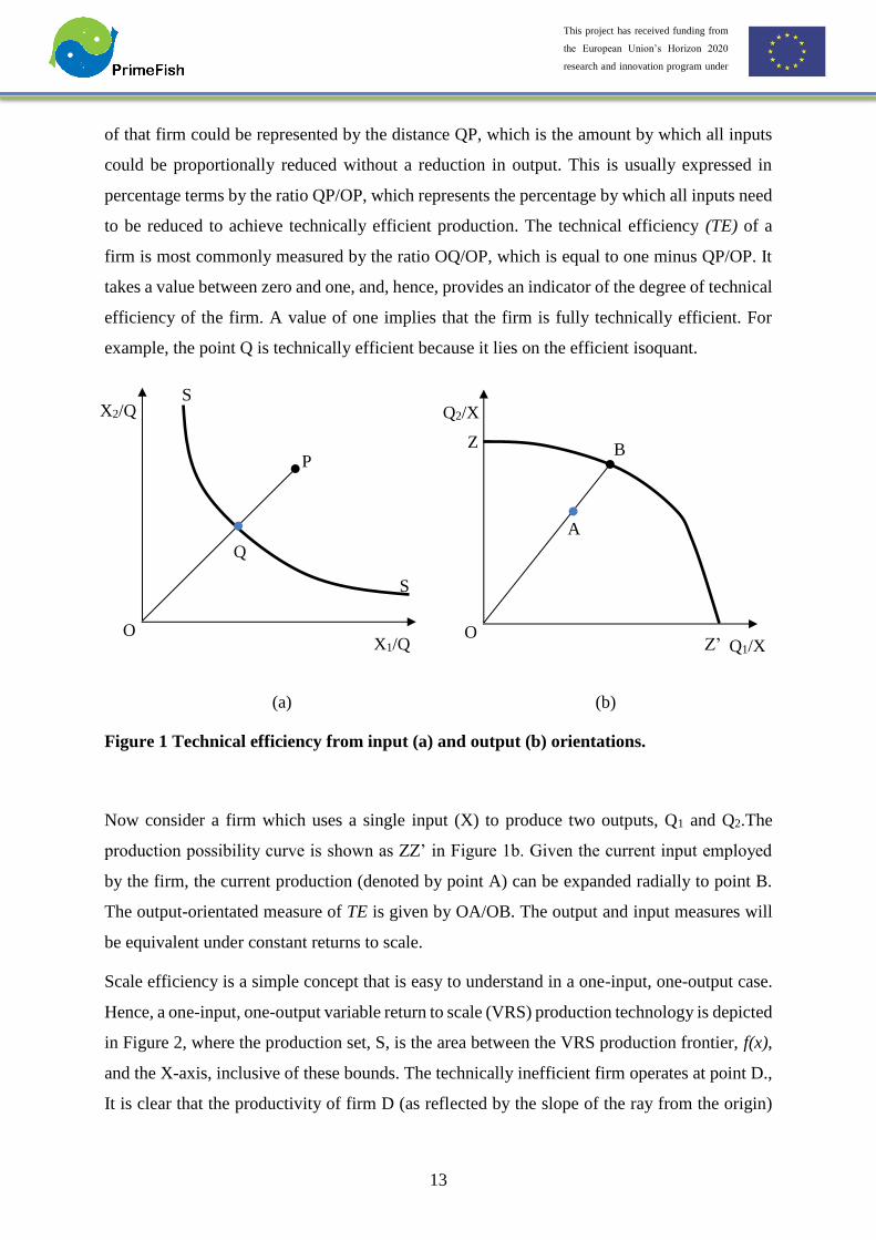
Following Farrell (1957), the input-orientation can be illustrated using a firm producing a single

output (Q) with two inputs (X1 and X2) under an assumption of constant returns to scale (CRS).

The isoquant of a fully efficient firm is given by SS’ in Figure 19a. If a given firm uses

quantities of inputs, defined by the point P, to produce a unit of output, the technical inefficiency

13





of that firm could be represented by the distance QP, which is the amount by which all inputs

could be proportionally reduced without a reduction in output. This is usually expressed in

percentage terms by the ratio QP/OP, which represents the percentage by which all inputs need

to be reduced to achieve technically efficient production. The technical efficiency (TE) of a

firm is most commonly measured by the ratio OQ/OP, which is equal to one minus QP/OP. It

takes a value between zero and one, and, hence, provides an indicator of the degree of technical

efficiency of the firm. A value of one implies that the firm is fully technically efficient. For

example, the point Q is technically efficient because it lies on the efficient isoquant.

(a) (b)

Figure 1 Technical efficiency from input (a) and output (b) orientations.

Now consider a firm which uses a single input (X) to produce two outputs, Q1 and Q2.The

production possibility curve is shown as ZZ’ in Figure 1b. Given the current input employed

by the firm, the current production (denoted by point A) can be expanded radially to point B.

The output-orientated measure of TE is given by OA/OB. The output and input measures will

be equivalent under constant returns to scale.

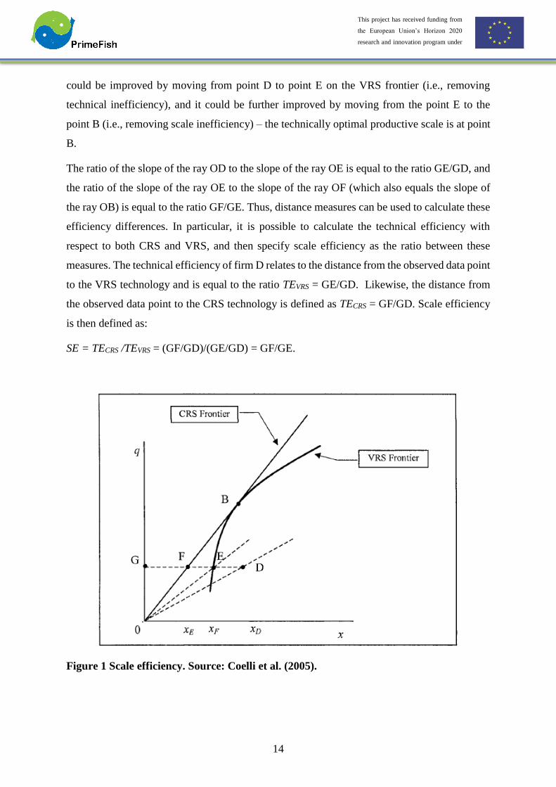
Scale efficiency is a simple concept that is easy to understand in a one-input, one-output case.

Hence, a one-input, one-output variable return to scale (VRS) production technology is depicted

in Figure 2, where the production set, S, is the area between the VRS production frontier, f(x),

and the X-axis, inclusive of these bounds. The technically inefficient firm operates at point D.,

It is clear that the productivity of firm D (as reflected by the slope of the ray from the origin)

Z’

Z

O

A

Q2/X

B

Q1/X X1/Q

X2/Q

O

Q

P

S

S

14





could be improved by moving from point D to point E on the VRS frontier (i.e., removing

technical inefficiency), and it could be further improved by moving from the point E to the

point B (i.e., removing scale inefficiency) – the technically optimal productive scale is at point

B.

The ratio of the slope of the ray OD to the slope of the ray OE is equal to the ratio GE/GD, and

the ratio of the slope of the ray OE to the slope of the ray OF (which also equals the slope of

the ray OB) is equal to the ratio GF/GE. Thus, distance measures can be used to calculate these

efficiency differences. In particular, it is possible to calculate the technical efficiency with

respect to both CRS and VRS, and then specify scale efficiency as the ratio between these

measures. The technical efficiency of firm D relates to the distance from the observed data point

to the VRS technology and is equal to the ratio TEVRS = GE/GD. Likewise, the distance from

the observed data point to the CRS technology is defined as TECRS = GF/GD. Scale efficiency

is then defined as:

SE = TECRS /TEVRS = (GF/GD)/(GE/GD) = GF/GE.

Figure 1 Scale efficiency. Source: Coelli et al. (2005).

15





The basic data envelopment analysis (DEA) model was defined by Charnes et al. (1978), based

on Farrell (1957). DEA models can be formulated for input minimization or output

maximization problems. As the calculations in this deliverable are all based on input

minimization, we will in what follows only outline that approach.

TE scores of decision-making units (DMU) are derived by estimating each separate frontier for

each year, by solving the following input-oriented DEA models:

Input-oriented DEA model under CRS assumption

TE = Min𝜃,𝜆 𝜃

Subject to 𝜃𝑥𝑖𝑗 − ∑ 𝜆𝑗𝑥𝑖𝑗 ≥ 0, 𝑖 = 1, … , 𝑀,𝑛𝑗=1

−𝑦𝑟𝑗 + ∑ 𝜆𝑗𝑦𝑟𝑗 ≥ 0, 𝑟 = 1, … , 𝑁, 𝑛𝑗=1

𝜆𝑗 ≥ 0, 𝑗 = 1, … , 𝑛,

(2)

Input-oriented DEA models under VRS assumption

TE = Min𝜃,𝜆 𝜃

Subject to 𝜃𝑥𝑖𝑗 − ∑ 𝜆𝑗𝑥𝑖𝑗 ≥ 0, 𝑖 = 1, … , 𝑀,𝑛𝑗=1

−𝑦𝑟𝑗 + ∑ 𝜆𝑗𝑦𝑟𝑗 ≥ 0, 𝑟 = 1, … , 𝑁, 𝑛𝑗=1

∑ 𝜆𝑗𝑛𝑗=1 = 1,

𝜆𝑗 ≥ 0, 𝑗 = 1, … , 𝑛,

(3)

where 𝑥𝑖𝑗 is the level of input i used by DMUj, 𝑦𝑟𝑗 is output r of the DMUj and 𝑛 is the number

of observed companies. The value of 𝜃 obtained is the efficiency score for the j-th firm. It

satisfies: 𝜃 ≤ 1, with a value of 1 indicating a point on the frontier and hence a technically

efficient firm.

The Malmquist Index (MI) is used to measure the total factor productivity (TFP) change of a

company or an industry over time, which is known as the Malmquist TFP index. If the MI

equals one, it represents no change in productivity; a value greater than one indicates positive

TFP growth; and an MI smaller than one indicates a TFP decline. The MI will be defined by

distance functions. The input distance function, which involves the scaling of the input vector,

is defined on the input set, L(q), as:

16





𝑑𝑖(𝒙, 𝒒) = max {𝜌: (𝒙

𝜌) ∈ 𝐿(𝒒)}, (4)

where the input set L(q) represents the set of all input vectors, x, which can produce the output

vector, q. The input distance function is illustrated using Figure 19a. The value of the distance

function for the point, P, is equal to the ratio ρ=OP/OQ (Figure 19a). The input-orientated TE

measure of a firm like (1) can be expressed in terms of input-distance function

𝑑𝑖(𝒙, 𝒒) as: 𝑇𝐸 = 1/𝑑𝑖(𝒙, 𝒒).

The input-orientated productivity measures focus on the level of inputs necessary to produce

observed output vectors 𝒒𝒕 and 𝒒𝒕+𝟏 under a reference technology. The input-orientated MI is

defined as:

𝑀𝑖(𝒒𝑡, 𝒒𝑡+1, 𝒙𝑡, 𝒙𝑡+1) = [𝑀𝑖𝑡(𝒒𝑡, 𝒒𝑡+1, 𝒙𝑡, 𝒙𝑡+1)𝑀𝑖

𝑡+1(𝒒𝑡, 𝒒𝑡+1, 𝒙𝑡, 𝒙𝑡+1)]12

= [𝑑𝑖

𝑡(𝒒𝑡+1, 𝒙𝑡+1)

𝑑𝑖𝑡(𝒒𝑡, 𝒙𝑡)

×𝑑𝑖

𝑡+1(𝒒𝑡+1, 𝒙𝑡+1)

𝑑𝑖𝑡+1(𝒒𝑡, 𝒙𝑡)

]

12

(5)

The MI in (4) is defined in terms of four input distance functions, and a separate Mi will be

calculated for every DMU. The MI formula can be decomposed in a common way as follow:

𝑀𝑖(𝒒𝑡, 𝒒𝑡+1, 𝒙𝑡, 𝒙𝑡+1) =𝑑𝑖

𝑡+1(𝒒𝑡+1, 𝒙𝑡+1)

𝑑𝑖𝑡(𝒒𝑡, 𝒙𝑡)

[𝑑𝑖

𝑡(𝒒𝑡+1, 𝒙𝑡+1)

𝑑𝑖𝑡+1(𝒒𝑡+1, 𝒙𝑡+1)

×𝑑𝑖

𝑡(𝒒𝑡, 𝒙𝑡)


]

12

(6)

or

𝑀𝐼 = 𝐸𝐶 × 𝑇𝐶,

where

𝐸𝐶 =𝑑𝑖

𝑡+1(𝒒𝑡+1, 𝒙𝑡+1)

𝑑𝑖𝑡(𝒒𝑡 , 𝒙𝑡)

(7)

𝑇𝐶 = [𝑑𝑖

𝑡(𝒒𝑡+1, 𝒙𝑡+1)

𝑑𝑖𝑡+1(𝒒𝑡+1, 𝒙𝑡+1)

×𝑑𝑖

𝑡(𝒒𝑡, 𝒙𝑡)


]

12

(8)

17





The decomposition given in (6) identifies two sources of productivity change. The first part is

technical efficiency change (EC) in (7). The second part is a measure of technical change (TC)

in (7), the movements of the frontier technologies between the two periods, and its contribution

to total productivity change.

Technical efficiency change (EC) be decomposed into scale efficiency change (SEC) and pure

technical efficiency change (PEC). This can only be done when the distance functions in the

above equations are estimated relative to a CRS technology (Fare et al.1994).

For the calculations, four different DEA models must be solved for each DMU. Assuming

constant returns to scale (CRS) to start with, the following input-orientated linear programs are

used:

[𝑑𝑖𝑡(𝒒𝑡, 𝒙𝑡)]−1 = Min𝜃,𝜆 𝜃

Subject to 𝜃𝑥𝑖𝑗,𝑡 − ∑ 𝜆𝑗𝑥𝑖𝑗,𝑡 ≥ 0, 𝑖 = 1, … , 𝑀,𝑛𝑗=1

−𝑦𝑟𝑗,𝑡 + ∑ 𝜆𝑗𝑦𝑟𝑗,𝑡 ≥ 0, 𝑟 = 1, … , 𝑁, 𝑛𝑗=1

𝜆𝑗 ≥ 0, 𝑗 = 1, … , 𝑛,

(9)

[𝑑𝑖𝑡+1(𝒒𝑡+1, 𝒙𝑡+1)]−1 = Min𝜃,𝜆 𝜃

Subject to 𝜃𝑥𝑖𝑗,𝑡+1 − ∑ 𝜆𝑗𝑥𝑖𝑗,𝑡+1 ≥ 0, 𝑖 = 1, … , 𝑀,𝑛𝑗=1

−𝑦𝑟𝑗,𝑡+1 + ∑ 𝜆𝑗𝑦𝑟𝑗,𝑡+1 ≥ 0, 𝑟 = 1, … , 𝑁, 𝑛𝑗=1

𝜆𝑗 ≥ 0, 𝑗 = 1, … , 𝑛,

(10)

[𝑑𝑖𝑡+1(𝒒𝑡, 𝒙𝑡)]−1 = Min𝜃,𝜆 𝜃

Subject to 𝜃𝑥𝑖𝑗,𝑡 − ∑ 𝜆𝑗𝑥𝑖𝑗,𝑡+1 ≥ 0, 𝑖 = 1, … , 𝑀,𝑛𝑗=1

−𝑦𝑟𝑗,𝑡 + ∑ 𝜆𝑗𝑦𝑟𝑗,𝑡+1 ≥ 0, 𝑟 = 1, … , 𝑁, 𝑛𝑗=1

𝜆𝑗 ≥ 0, 𝑗 = 1, … , 𝑛,

(11)

[𝑑𝑖𝑡(𝒒𝑡+1, 𝒙𝑡+1)]−1 = Min𝜃,𝜆 𝜃

Subject to 𝜃𝑥𝑖𝑗,𝑡+1 − ∑ 𝜆𝑗𝑥𝑖𝑗,𝑡 ≥ 0, 𝑖 = 1, … , 𝑀,𝑛𝑗=1

−𝑦𝑟𝑗,𝑡+1 + ∑ 𝜆𝑗𝑦𝑟𝑗,𝑡 ≥ 0, 𝑟 = 1, … , 𝑁, 𝑛𝑗=1

𝜆𝑗 ≥ 0, 𝑗 = 1, … , 𝑛,

(12)

The first two linear programs in (9) and (10) are where the technology and the observation to

be evaluated are from the same period, and the solution value is less than or equal to unity. The

second two linear programs in (11) and (12) occur where the reference technology is

18





constructed from data in one period, whereas the observation to be evaluated is from another

period.

DEA fits well the datasets used in D2.3 and meets one of the tasks of the work package’s aim

to understand economic performance at firm level. It is possible to apply another method such

as stochastic frontier analysis (SFA), which is a method of economic modeling that applies

regression technique to estimate parameters of production inputs. However, DEA has the

following important advantages:

• Can handle multiple input and multiple output models.

• Does require an assumption of a functional form relating inputs to outputs.

• Firms are directly compared against other firms or combination of firms. In this case,

DEA provides clear results for comparing efficiency among pangasius, salmon and

seabass/seabream firms.

• Inputs and outputs can have very different units.

The same characteristics that make DEA a powerful tool can also create problems. Thus:

• Since DEA is an extreme point technique, noise (even symmetrical noise with zero

mean) such as measurement error can cause significant problems.

• DEA is good at estimating "relative" efficiency of a firm but it converges very slowly

to "absolute" efficiency. In other words, it can tell you how well you are doing

compared to your peers but not compared to a "theoretical maximum."

• Since DEA is a nonparametric technique, statistical hypothesis tests are difficult and

are the focus of ongoing research.

• Since a standard formulation of DEA creates a separate linear program for each firm,

large problems can be computationally intensive.

The farmed fish-datasets at firm level have a number of weaknesses that limit the choice of

methodology as well the analysis undertaken. The datasets do not include equal number of firms

(decision making units), time periods are not the same for all datasets, and inputs and outputs

vary between data sets. This makes it impossible to compare the DEA results across case

studies.

19





Future research may apply DEA for another datasets. For example, DEA is now sometimes

used for analysis of survey data at firm level. The firm questionnaire can be generated with

identical output and input variables deployed for different case studies. The identical input and

output variable enable the comparisons of economic performance between aquaculture sectors

as well as across firms within sectors. The surveyed data are also more recent than the time

series data. However, surveyed data can rarely be used to analyse changes in productivity and

efficiency over times.

20





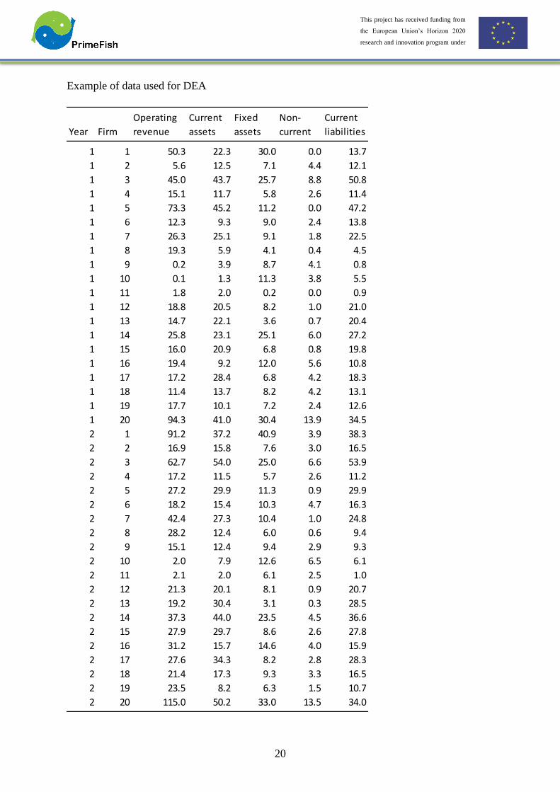
Example of data used for DEA

Year Firm

Operating

revenue

Current

assets

Fixed

assets

Non-

current

Current

liabilities

1 1 50.3 22.3 30.0 0.0 13.7

1 2 5.6 12.5 7.1 4.4 12.1

1 3 45.0 43.7 25.7 8.8 50.8

1 4 15.1 11.7 5.8 2.6 11.4

1 5 73.3 45.2 11.2 0.0 47.2

1 6 12.3 9.3 9.0 2.4 13.8

1 7 26.3 25.1 9.1 1.8 22.5

1 8 19.3 5.9 4.1 0.4 4.5

1 9 0.2 3.9 8.7 4.1 0.8

1 10 0.1 1.3 11.3 3.8 5.5

1 11 1.8 2.0 0.2 0.0 0.9

1 12 18.8 20.5 8.2 1.0 21.0

1 13 14.7 22.1 3.6 0.7 20.4

1 14 25.8 23.1 25.1 6.0 27.2

1 15 16.0 20.9 6.8 0.8 19.8

1 16 19.4 9.2 12.0 5.6 10.8

1 17 17.2 28.4 6.8 4.2 18.3

1 18 11.4 13.7 8.2 4.2 13.1

1 19 17.7 10.1 7.2 2.4 12.6

1 20 94.3 41.0 30.4 13.9 34.5

2 1 91.2 37.2 40.9 3.9 38.3

2 2 16.9 15.8 7.6 3.0 16.5

2 3 62.7 54.0 25.0 6.6 53.9

2 4 17.2 11.5 5.7 2.6 11.2

2 5 27.2 29.9 11.3 0.9 29.9

2 6 18.2 15.4 10.3 4.7 16.3

2 7 42.4 27.3 10.4 1.0 24.8

2 8 28.2 12.4 6.0 0.6 9.4

2 9 15.1 12.4 9.4 2.9 9.3

2 10 2.0 7.9 12.6 6.5 6.1

2 11 2.1 2.0 6.1 2.5 1.0

2 12 21.3 20.1 8.1 0.9 20.7

2 13 19.2 30.4 3.1 0.3 28.5

2 14 37.3 44.0 23.5 4.5 36.6

2 15 27.9 29.7 8.6 2.6 27.8

2 16 31.2 15.7 14.6 4.0 15.9

2 17 27.6 34.3 8.2 2.8 28.3

2 18 21.4 17.3 9.3 3.3 16.5

2 19 23.5 8.2 6.3 1.5 10.7

2 20 115.0 50.2 33.0 13.5 34.0

21





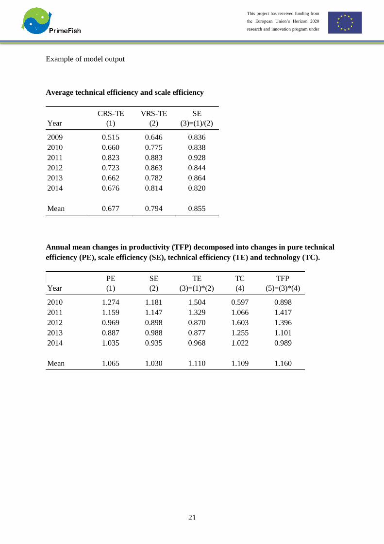
Example of model output

Average technical efficiency and scale efficiency

Annual mean changes in productivity (TFP) decomposed into changes in pure technical

efficiency (PE), scale efficiency (SE), technical efficiency (TE) and technology (TC).

CRS-TE VRS-TE SE

Year (1) (2) (3)=(1)/(2)

2009 0.515 0.646 0.836

2010 0.660 0.775 0.838

2011 0.823 0.883 0.928

2012 0.723 0.863 0.844

2013 0.662 0.782 0.864

2014 0.676 0.814 0.820

Mean 0.677 0.794 0.855

PE SE TE TC TFP

Year (1) (2) (3)=(1)*(2) (4) (5)=(3)*(4)

2010 1.274 1.181 1.504 0.597 0.898

2011 1.159 1.147 1.329 1.066 1.417

2012 0.969 0.898 0.870 1.603 1.396

2013 0.887 0.988 0.877 1.255 1.101

2014 1.035 0.935 0.968 1.022 0.989

Mean 1.065 1.030 1.110 1.109 1.160

22





4 Kalman filter

The methodology discussed in this section was used in two deliverables, D2.4 and D5.2, both

of whom deal with the analysis of “boom-and-bust cycles”. The statistical model used for the

identification of cycles in the time series is the Kalman filter. The starting approach is to look

at a time series with the approach of structural models (Harvey, 1989). The traditional approach

to the analysis of time series is to decompose the observed values as the sum of a linear or

quadratic trend, a fixed cycle and a seasonal component modelled using a set of dummy

variables or harmonics and an irregular component and eventually a set of fixed explanatory

variables. However, when these components are not stable this formulation becomes inadequate

and it is necessary to allow them to change over time. This flexibility is possible with structural

models, such that "they are not more than regression models in which explanatory variables are

a function of time and the parameters change with time" (Harvey, 1989). One peculiarity of a

structural model is its flexibility in recognizing changes in the behaviour of a given series, by

taking its different components as stochastic processes governed by random disturbances.

The Kalman filter decomposes the time series into elementary parts such as trend, cycle,

seasonality and irregular component. Trend is defined as any long term tendency. By extension,

the trend is the fundamental tendency (towards the increasing, the reduction or even to price

stability) that the activities of the fisheries sector in periods of varying length (but always groups

of years), apart from accidental variations (irregularities or outliers), seasonal and cyclical. The

cycle (or cyclical component) is defined as alternation of different sign fluctuations around the

trend. Seasonal component consists of changes that occur with similar intensity in the same

periods every year, but with different intensity in the course of a year (for example, production

is falling every year in the summer following the holiday closure of many companies, but it

increases every year as Christmas approaches to and greater consumption). The irregular

component represents unforeseeable and accidental variations related to all the most varied

types of events. This component in some cases, may include extreme values or outliers.

The Kalman filter as well as break down the price trend in building blocks may be allocated to

each member of the characteristics of stochasticity and determination. The classification of a

component as a stochastic or deterministic is of particular importance since it allows to

understand more in detail what inside on the price trend analysis can be considered as "fixed"

or "probabilistic". The Kalman filter also allows to determine if the individual components are

stochastic or deterministic

23





In order to estimate the parameters of the structural time series models it is necessary to put

them inside the so called state-space form and then apply the Kalman filter. The filter has its

origin in Kalman’s (1960) paper who describes a recursive solution to the linear filtering

problem of discrete data. Kalman’s derivation took place within the context of state-space

models, whose core is the recursive least squares estimation. The state-space representation is

essentially a convenient notation to estimate stochastic models in which one assumes

measurement errors in the system which allows handling a large set of time series models. The

filter is a mathematical tool which operates by means of a prediction and correction mechanism.

Essentially, this algorithm predicts the new state (which contains all information up to that point

in time) starting from a previous estimation and adding a proportional correcting term to the

prediction error, such that the latter is statistically minimized. The complete estimation

procedure is as follows: the model is formulated in state-space form and for a set of initial

parameters, the model prediction errors are generated from the filter. These are then used to

recursively evaluate the likelihood function until it is maximized. The Kalman filter comprises

a set of mathematical equations which result from an optimal recursive solution given by the

least squares method. The purpose of this solution consists in computing a linear, unbiased and

optimal estimator of a system’s state at time t, based on information available at t - 1 and update,

with the additional information at t, these estimates (Clark et al. 1998). The filter’s performance

assumes that a system can be described through a stochastic linear model with an associated

error following a normal distribution with mean zero and known variance. The solution is

optimal provided the filter combines all observed information and previous knowledge about

the system’s behaviour such that the state estimation minimizes the statistical error. The

recursive term means that the filter re-computes the solution each time a new observation is

incorporated into the system.

The Kalman filter is the main algorithm to estimate all structural models written in state-space

form (Harvey and Proietti, 2005). This representation of the system is described by a set of state

variables. The state contains all information relative to that system at a given point in time. This

information allows to infer about the past behaviour of the system, aiming at predict its future

behaviour. What makes the Kalman filter so interesting is its ability to predict the past, present

and future state of a system, even when the precise nature of the modelled system is unknown.

In practical terms, the individual state variables of a dynamic system cannot be exactly

determined through a direct measurement. In this context, their measurement is done by means

of stochastic processes involving some degree of uncertainty.

24





Data were also used in the report to analyse the price transmission and market integration for

selected species. Price transmission refers to the process in which upstream (producer) prices

affect downstream (retail) prices. The relationships between different stages in the value chain

(upstream and downstream), based on a simultaneous equilibrium, have been described by the

theory of derived demand. The absence of complete pass-through of price changes and costs

from one market to another has important implications for economic welfare. Price transmission

studies provide important insights into how changes in one market are transmitted to another,

and consequently reflect the extent to which markets function efficiently.

The main objective of D2.4 was to estimate the presence of boom and bust cycles and the best

model for cycle analysis using the Kalman filter due to its ability to isolate the cycle component

from other components. In addition, the filter highlights the irregular component of the cycle

that allows us to determine how much what we are observing is stochastic or deterministic,

allowing us to evaluate the goodness of the results obtained.

With the support of the economics literature (Gerdesmeier et al., 2012), and through many tests

performed on the data, it seemed reasonable to argue that we can talk about boom or bust if

prices are greater than the 85th percentile or below the 15th percentile. Furthermore, in order

to avoid false signals, we classify a set of values beyond thresholds as a group if inside the set

we do not have more than three consecutive monthly observations below the thresholds. This

method allows avoidance of the formation of two booms or two busts in close periods just

because there is a single value in the set that falls inside the percentiles used as a threshold. The

classification method used to reduce the false signals produces smoother cycles.

The methodology applied is coherent with the current development of the international research

in this field. However, other methodology could have been applied. Some examples include:

• ARCH (autoregressive conditionally heteroscedastic) model is a model for the

variance of a time series. ARCH models are used to describe a changing, possibly

volatile variance. Although an ARCH model could possibly be used to describe a

gradually increasing variance over time, most often it is used in situations in which

there may be short periods of increased variation.

• GARCH (generalized autoregressive conditionally heteroscedastic) model uses

values of the past squared observations and past variances to model the variance

at time t.

25





The algorithm of the Kalman filter has several advantages. This is a statistical technique that

adequately describes the random structure of experimental measurements. This filter is able to

take into account quantities that are partially or completely neglected in other techniques (such

as the variance of the initial estimate of the state and the variance of the model error). It provides

information about the quality of the estimation by providing, in addition to the best estimate,

the variance of the estimation error.

The Kalman filter is very useful in this contest as it is able to identify the cycles, if they exist,

to determine their length and to provide a diagnostic index of statistical significance.

The disadvantages of the method are mainly that it provides accurate results only for Gaussian

and linear models.

The methodology applied in D2.4 was directly based on the type of data collected and based on

the objective of the task. The model applied, in our opinion, provides the best possible estimate

for the cycle in prices time series for the species analysed.

The methods used in the D2.4 are quite robust and applied widely. However, there are still

rooms to improve the application. For example, data are sufficient to investigate deeply the

price transmission and market integration by advanced techniques such as cointegration

analysis. Cointegration analysis can be applied to develop an empirical model that aims to test

market integration and price leadership between actors in the value chain of seafood species. It

is also possibly applied to test the horizontal market integration and market leadership among

species. In addition, the quantile regression technique may be extended to empirical model by

involving the deterministic variables of macro-economic factors (e.g., average income, interest

rate, exchange rate, and national economic growth). The Kalman filter method may be applied

more intensively by further investigating the stochastic components of the prices. These

recommendations are suggested for future studies.

26





Example of data collected

year month_of_year year-month countrymain_commercial_species weighted_price market

2010 12010-1 United Kingdom Cod 7,31retail2010 22010-2 United Kingdom Cod 7,31retail2010 32010-3 United Kingdom Cod 7,01retail2010 42010-4 United Kingdom Cod 7,08retail2010 52010-5 United Kingdom Cod 7,31retail2010 62010-6 United Kingdom Cod 7,66retail2010 72010-7 United Kingdom Cod 7,52retail2010 82010-8 United Kingdom Cod 7,74retail2010 92010-9 United Kingdom Cod 7,5retail2010 102010-10 United Kingdom Cod 7,22retail2010 112010-11 United Kingdom Cod 7,5retail2010 122010-12 United Kingdom Cod 7,56retail2011 12011-1 United Kingdom Cod 7,71retail2011 22011-2 United Kingdom Cod 7,56retail2011 32011-3 United Kingdom Cod 7,42retail2011 42011-4 United Kingdom Cod 7,36retail2011 52011-5 United Kingdom Cod 7,4retail2011 62011-6 United Kingdom Cod 7,27retail2011 72011-7 United Kingdom Cod 7,6retail2011 82011-8 United Kingdom Cod 7,48retail2011 92011-9 United Kingdom Cod 7,6retail2011 102011-10 United Kingdom Cod 7,84retail2011 112011-11 United Kingdom Cod 7,84retail2011 122011-12 United Kingdom Cod 8,19retail

27





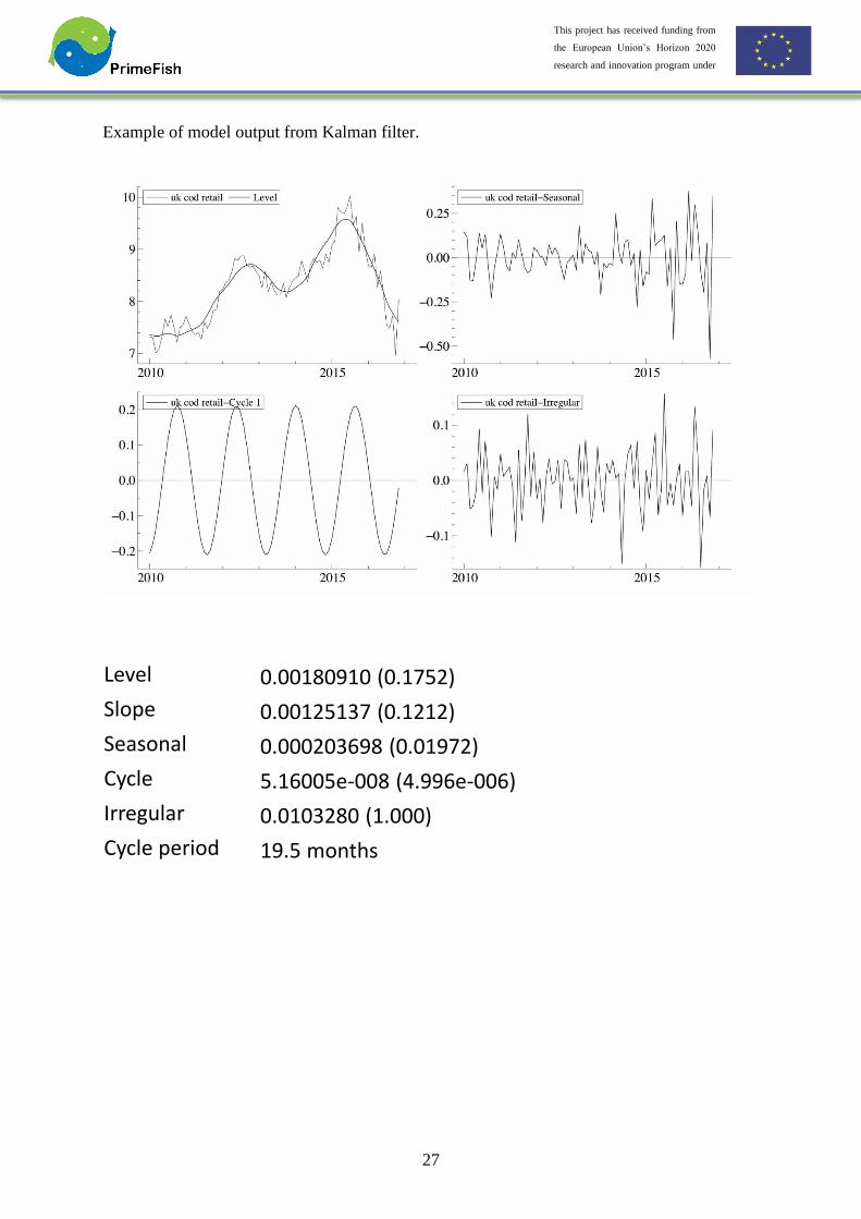
Example of model output from Kalman filter.

Level 0.00180910 (0.1752)

Slope 0.00125137 (0.1212)

Seasonal 0.000203698 (0.01972)

Cycle 5.16005e-008 (4.996e-006)

Irregular 0.0103280 (1.000)

Cycle period 19.5 months

28





5 Price transmission and market integration

In Task 2.3.3, price co-integration was employed to analyse price transmission and market

integration between species, among markets and along the value chains, i.e. between farming

and processing sectors. The methodology is based on Nielsen et al. (2009)

The general formulation is driven by the empirical evidence is that there is strong support to

use a Granger causal model (mixed with Autoregressive Moving Average [ARMA] model)

However the effect of lagged causality of X(t-1) over Y(t) can be hidden as absorbed by the

time-evolution modelled with the ARMA model. The formal definition of the ARMA model

with the explanatory variable is

Yt = c + ϕ1Y{t−1} + θ1ϵ{t−1} + γ0Xt + γ1X{t−1} + ϵt,

where ϵt is a White Noise (assumed Gaussian) error term. The model can be used only when

first sale price and retail price are both available for a sufficiently long time period (with

monthly data) and no missing data. So, in the sequel, only combinations of fish/country where

these restrictions are met will be under investigation.

Under the model assumptions it is expected that changes in X will cause changes in Y. This

cause-effect transmision works if the time series share, at least, a mild common pattern (i.e. Y

is large when X is large and vice-versa) and have a kind of long-term steady mean-stationary.

The parameter c and γ0 are probably the two most important in terms of economic

interpretation. The constant c is the fixed mark-up and γ0 is the proportional mark-up

(elasticity). Price transmission elasticity is defined as “the relative change in retail price to the

relative change in producers’ price when other factors affecting processors behaviour are held

constant”. So, the elasticity of price transmission measures the percentage change in the price

at a downstream stage of the market chain, in relation to the relative change in the price of the

same product at an upstream stage in the market chain.

The statistical hypothesis will assess the significance of the parameters via their p-value and

only relevant parameters will be included. The comments to parameters will be mostly

economical referred to the magnitude at which the prices are transmitted from first sale to retail.

When common trend are found a modification to the above model will take into account the

cointegration term.

29





The methodology was chosen because it is an advanced generalization to causal models that

were analysed in the literature cited below. It exploits cause-and-effect and uses robust

estimations.

This is the standard methodology used for this type of analysis, but has been enhanced by new

robust estimators. Other methodologies could rely on a fully complete state-space

representation to deal with irregularly samples time series.

The model is flexible enough to deal with seasonal, cyclical and erratic behaviours. Good out-

of-sample forecasts and ease of interpretation. However, it can only be applied to regularly

based time-series. Missing values create troubles and restrict the analysis to some datasets.

The objective of the task and the type of data collected dictated the methodology used. The

model applied provided, in our opinion, the best possible results.

Future studies using similar methodology should take car to collect the data using a proper

pre-defined methodology in a well organised database. The data used in this study are taken

from EUMOFA and include the following variables: year, month of year, average monthly

prices.

30





6 Global value chain analysis

Global value chain (GVC) analysis has been used as the underlying framework for the

deliverables undertaken in work package 3. GVC mapping and quantification of “input-output

structure“ are standard initial steps of value chain analysis (Kaplinsky & Morris, 2001). A

holistic VCA is conceived in PrimeFish as four inter-linked elements with focus on

competitiveness (see T3.4 Deliverable Protocol). D3.1 represents the first of these steps, while

the other linked elements of VCA can be found in D3.2 value chain governance, D3.3 market

based governance, D3.4 Industry dynamics, opportunities and threats and to some extent in

D4.1 product innovation case studies.

The initial data analysis was performed by each partner institution responsible for the value

chain case and detailed in the form of a report on the structure of the respective value chain.

Each report separately describes the main material flow in the supply chain (mapping and input-

output structure description) for one of the six commodity species (or species groups) that are

the focus of PrimeFish; four farmed and two capture: (i) Atlantic Salmon, (ii) Rainbow Trout,

(iii) European Sea bass (Dicentrarchus labrax) and gilthead sea bream (Sparus aurata) (iv)

Pangasius catfish (Pangasius hypophthalmus) (v) Atlantic Cod (Gadus morhua) (vi) Atlantic

Herring (Clupea herrengus). The latter two species are selected as examples of demersal and

pelagic fisheries. Sea bass and sea bass are treated as a single group as almost perfect

substitutes, sharing very similar production and post-harvest value-chain characteristics.

The value chain mapping started at the production node of the VC in the selected country of

interest to PrimeFish (reasons for selection of countries detailed elsewhere), and traced the

material downstream to processing (primary and/or secondary), marketing and consumption

within the domestic portion of the value chain, exports to other markets and imports. As a first

step the analysis positions the producer country on the global scene, particularly relevant for

internationally traded commodities. Then it covers the volume and value of outputs from each

major node in the value chain (raw material production, processing, distribution, retail and food-

service, where data were available). The analysis was furthered through quantifying the

additional elements of the VC detailed below.

1. Supply of material

a. Landing/production

31





i. structure – for national fleet: number of vessels, size and capacity,

employment, if possible with relevance to the type of fisheries

(demersal or pelagic); for aquaculture - number of plants (possibly

types within the production chain: hatcheries, nurseries, and for

consumption/restocking; sizes, employment

ii. Landings (LWE and/or landed weight for domestic and foreign fleet);

volume and value, price per kg; production capacity of aquaculture:

eggs laid, seed (fry, fingerling) produced, fish for consumption -

volume and value, price per kg

b. Imports

i. Eggs and seed (for aquaculture) – number and value

ii. Raw material/products imported (by category) – volume and value

iii. Main exporting countries – volumes and value

2. Processing

a. Types of raw materials raw materials supplied, volumes, values and prices for

different processor types (primary, secondary, mixed)

b. Outputs – types of products, volumes and value

c. Gross value added (GVA)

3. Consumption and Export

a. Retail sector – retail volumes, value of sales, average retail prices, GVA where

available

b. Food Service sector - retail volumes, value of sales, average retail prices, GVA

where available

c. Export – types of products exported, volumes and values, countries of

destination.

Since the aim of this exploratory analysis was to summarize and visualize data, only simple

data manipulations were performed e.g. totals, proportion, growth rate etc.

In most of cases the available data covered the period 2000-2014 at annual intervals, the

analysis allowed identification of major trends in time and patterns across locations. A further

synthesis was performed of the 17 individual value-chain descriptions, utilising a cross-case

analyses i.e. each case (country VC) is compared to the other cases of the same type (species)

32





in order to draw broad conclusions as to what the important aspects of this value chain were

which define its structure, which forms and can be found in D3.1. The identification of these

components served as a guide to further analysis and in-depth exploration of these issues in

D3.4 with particular focus on competitiveness.

Competition is a complex, dynamic and multi-dimensional concept, while the global economy

is increasingly structured around global value chains (GVCs) that account for a rising share of

international trade, global GDP and employment (Gereffi & Fernandez-Stark, 2011). The major

outputs of the EU‘s fisheries and aquaculture industries are no exception: the selected species

of focus to PrimeFish represent internationally (globally) traded commodities. The multi-

dimensionality and international scope of competition of EU fisheries and aquaculture, call for

a systems thinking approach (Wächter, 2011) which lies at the core GVC analysis.

The activities that comprise a value chain can be contained within a single firm or divided

among different firms (globalvaluechains.org, 2011). In the context of globalization, the

activities that constitute a value chain have generally been carried out in inter-firm networks on

a global scale.

Gereffi & Fernandez-Stark (2011) describe six basic dimensions that GVC methodology

explores, divided into global and local elements. The analysis of this dataset comprises the first

two dimensions (1) an input-output structure, which describes the process of transforming raw

materials into final products and (2) the geographic scope, which explain how the industry is

globally dispersed and in what countries the different GVC activities are carried out. These

dimensions are concerned primarily with a ‘global’ analysis level of analysis (a more ‘local’

level analysis i.e. at national industry and company level is covered in D3.4)

Primarily descriptive statistical approaches were used since the aim of this initial analysis was

collation/ exploration of available data including identification of major trends.

Globalization has given rise to a new era of international competition that is best understood by

looking at the global organization of industries and how countries rise and fall within these

industries. The global value chain framework has evolved from its academic origins to become

a major paradigm used by a wide range of country governments and international organizations,

including the World Bank, the International Labour Organization, the U.K. Department for

International Development, and the U.S. Agency for International Development. Global value

chain analysis highlights how new patterns of international trade, production, and employment

33





shape the prospects for development and competitiveness, using core concepts like

“governance” and “upgrading” (Gereffi & Fernandez-Stark, 2011).

The GVC is a framework for analysis which is flexible and allow addition of different „lenses“

(e.g. competition, gender, environment) to suit the needs of the analysis and the intended users

of the research (Bolwig, Ponte, du Toit Riisgaard, Lone, & Halberg, 2010). It is also flexible in

terms of the choice of qualitative or qualitative methods, or a combination thereof.

The integrated framework underpinning this WP combine elements from the Global value chain

school (primarily Gereffi) and the Strategic Management and industrial economics schools (e.g.

(McGahan, 2000; Porter, 1980, 1998; Rumelt, 1991). The flexibility of the GVC framework

makes is particularly suitable for this type of analysis, and a better candidate to narrower

approaches such as single industries.

In value chain mapping it is important to generate data over time, showing the trajectory of

change as well as the position in any one point in time. An alternative approach would have

been a more qualitative analysis of trends, however, that would have not allowed graphical

visualisation of trends.

Apart from the advantages of GVC mentioned above, the comprehensive nature of the

framework allows policy makers to answer questions regarding development issues that have

not been addressed by previous paradigms. It allows holistic understanding of how global

industries are organized by examining the structure and dynamics of different actors involved

in a given industry. GVC is a predominantly qualitative approach; the range validation steps

routinely applied in social research are therefore requirement to verify the robustness of

findings.

Initial scanning of data sources available in the public domain indicated GVC was a suitable

framework for the consequent collection and analysis of data. The flexibility of GVC allows

extending the analysis to different areas of interest where data are available, as well as adapting

to the contingent circumstances of the research investigation, recognising that not in all

researchers in the project will have equal access to data and importantly, the same quality of

access to the subjects of the research.

The use of framework approaches requires deep understanding of the underpinning theory and

ideally some level of relevant prior experience by all members of the team. Thus, extensive

training is required by to align the perspectives of what in cases may be a diverse range of

34





specialists. As such, this approach could be resource intensive in terms of supervision time. To

ameliorate this, where possible the elements of the approach should be standardized and used

in a prescriptive way.

Attempts to get access to internal company data on production (cut offs, waste etc.) or

economic data for the company quickly showed to close the open dialogue. When asking to

this type of information, the reaction were that this is confidential information, which could

be used by competitors. Bringing this up would close for the open dialogue about e.g.

relations in the value chain including relations to competitors and customers. – It is important

not to mix too much in approach. This seems to confuse the interview person in understanding

the purpose of the interview.

The economic/production data seems to be confidential for outsiders of the company. This

type of data can probably only be accessed based on long-term trust relation (the company

trust the interviewer not to share information with others unless real anonymised – e.g. in a

form that cannot be identified by persons knowing the industry and companies) or based on

official data collection under law and public guaranteed discretion.

35





7 Value-chains: Market institutional analysis

This analysis was used in D3.2. The data set used for this analysis were contained partly in

value chain mapping in D3.1 and in specific national working papers summarising the legal

institutional framework for fisheries and aquaculture. Further international (WTO) and EU

documents on trade agreements (including tariffs) as well as other regulation were used.

The national reports from partners were mainly based on literature review and limited number

of interviews with key informants. Themes for interviews (and literature reviews) were

developed in the project, but a common coding system was not developed. At national level the

interviews were coded for analysis. The common thematic focus was seen as productive for

ensuring comparable information between countries. Local coding allowed for openness for

including possible local aspects and perspectives. The national perspectives were used to further

focus (and in some cases broaden) the supranational analysis.

The supranational analysis was based on reports, legal documents including e.g. tariff

databases. Data from reports and other “grey” documents, interpretation of legal documents,

databases and the national interpretation of the supranational legal framework influencing the

competitiveness of the national seafood industry where combined in the analysis process. In

this process triangulation, using different sources and types of sources to enlighten the subject,

were used to substantiate the conclusions.

36





8 Value-chains: Labelling and certification

A holistic VCA is conceived in this project of four inter-linked elements with focus on

competitiveness (see T3.4 Deliverable Protocol), of which this task and associated database

represents D3.3 market based governance. The other linked elements of VCA can be found in

D3.1 Value chain descriptions, D3.2 value chain governance, D3.4 Industry dynamics,

opportunities and threats and to some extent in D4.1 product innovation case studies.

D3.3 addressed the current use and potential of voluntary market-based labelling and

certification schemes for different actors of the value-chain. Growth in the market for social

and environmentally assured seafood products has been driven by lead brands in the sector

adopting third-party certification and eco-labelling as a strategic-option for outsourcing

reputational risk management. This therefore represents an increasingly important facet in

competition strategy at company and sectoral levels.

The dataset compiled for this task comprises publicly available data from various sources

(including farm audit reports, certification websites and for the salmon sector, industry Global

Salmon Initiative (GSI) ‘sustainability reports’) on the aquaculture production node of the value

chain. It covers the following certification schemes:

• Aquaculture Stewardship Council (ASC)

• GlobalG.A.P.

• Best Aquaculture Practices (BAP)

• Friends of the Sea

And the following species groups and locations

• Salmonids (Atlantic salmon, coho salmon, rainbow trout, Arctic charr, brown trout) -

globally

• Sea bass and sea bream - globally

• Pangasius catfish – Viet Nam

37





Data from diverse sources were curated, standardized and organized in a relational database

which allowed using query functionality in addressing the research questions.

The analytical approach is descriptive in nature and includes trends analysis, market share

estimations, and strategy analysis, which are summarized and visualized in graphs, tables and

maps.

Based on a review of literature and media reports; the task also looks at the political economy

of the growing certification sector. Specifically market-failures associated with the dominance

of single scheme that achieved clear ‘first-mover’ advantage in the fisheries sector and the

proliferation of aquaculture standards and associated imposition of multiple-audit costs on

producers. Approaches for dealing with these market failures are also reviewed.

These analyses and interpretation of quantitative data was supported by semi-structured

interviews with representatives of industry and certification bodies.

Publicly available data on seafood certification is dispersed among a number of sources. A

holistic analysis is only possible when pooling the data together and standardizing them, in

order to uncover broader trends.

By positioning market-based governance as an element of value chain analysis we can build on

chain and network conceptualisations to better understand how private governance

arrangements are structured, and how such governance mechanisms can engage with chain

actors in influences over sustainability (Bush, Oosterveer, Bailey, & Mol, 2015).

The methodological mix was deemed to be most consistent with the research questions of this

task.

Collection of data from a diverse resource base, curation and standardisation is a time

consuming process. However, it allows the analysis of data otherwise existing in a non-

analysable form. The method also allows incorporation of further data (e.g. other species and

other certification schemes) into a standardised format for analysis.

The analysis as part of broader GVC framework allows holistic understanding of how global

industries are organized by examining the structure and dynamics of different actors involved

in a given industry.

The choice of methodology has been used in line with the research questions in this task.

Nevertheless more complete data would have allowed increasing the depth of analysis, through

38





answering further questions which are at this point not possible to answer because of data

limitations.

Request for data from relevant institutions met with mixed success. Lack of timely geographical

(GPS) data increased reliance on less time-efficient and potentially less accurate interpolation

of from publically available ‘certification maps’. Conversely industry contacts provided

generous access to GSI data-sets which would otherwise have had to be extracted piecemeal

from the GSI website.

39





9 Discrete choice analysis

This section describes the methodology applied in carrying out deliverable 3.5 on population

assessment and valuation of non-market effects (McFadden 1974; Hensher, Rose and Greene,

2007; Train, 2009; Hanley and Barbier, 2009).

Externalities are defined as “unintended effects of production (or consumption), which are

costly for the producer to neutralize”. Externalities can be of both positive and negative

character. An example of a negative externality of European fish production is the overfishing

of some fish stocks, which disturb the ecosystem these stocks are part of and thus these

ecosystems may be less productive than without overfishing. An example of a positive

externality we can find in some types of fish farming, where the waste from e.g. salmon

production can be used by scallops farms. While the outcome of the mentioned positive

externality is captured by economic agents and thus partly internalized, it is of less concern to

society than the negative externality, which imply costs inflicted upon the whole society,

without being compensated for. Hence, although we also will treat positive externalities, the

main focus will be on negative externalities of fish production.

We use two case study fish industries to exemplify the role and extent of externalities in

European fish production. These are production of farmed Atlantic salmon, and production

(harvest) of wild cod. By the use of a methodology called choice experiment, we analyze to

what extent case study producers are willing to internalise a few widely recognized

externalities. The results of this analysis should be seen in relation to results from WP4.4, which

is a choice experiment among European fish consumers. Taken together, the results from the

two surveys will convey information of whether consumers and producers of fish agree on

which are the important environmental issues in the European fish industry. Are fish producers

focusing on the “right” environmental issues, and are consumers willing to pay more for the

fish to encourage the producers to take environmental considerations?

For this deliverable, data is collected by the use of a survey questionnaire. Focal in this

questionnaire is a set of choice cards, asking the respondents to choose between three

alternatives for production of fish, where the alternatives are described by a combination of

economic and environmental attributes. Based on the choices the respondents make on the cards

the attributes characterizing the production process, which the respondents find most or least

important can be elicited. This is done by the use of statistical methods in the form of bi- or

multinomial logit models. The resulting, preference intensities for the attributes describing the

40





production process can be further developed to express willingness to pay (WTP), which

indicate what producers are willing to pay to improve each of the attributes describing the

production alternatives.

We have applied a combination of qualitative semi-structured interviews and quantitative

monetary valuation of sets of externalities relevant for each of the two fisheries production in

question (farmed Atlantic salmon and wild cod).

For each fishery we derived a choice experiment survey, including both qualitative questions

about main environmental issues, and choice cards. In the choice cards respondents were asked

to choose between three production alternatives, one of which describes a generalized present

situation and two which describes alternatives with lower environmental footprints, but higher

production costs.

Based on the choice cards it is possible to derive monetary valuation of the environmental issues

(named attributes). We do this by using the random utility model, assuming that the utility to a

fisher/fish farmer of a production alternative depends on a set of attributes describing the

environmental and other characteristics, including production costs. To take into account the

influence of random components on individual utility we also add an idiosyncratic i.i.d. error

term. Hence, utility of a production alternative j to respondent i can be formulated as follows;

𝑈𝑖𝑗𝑡(𝑏| 𝑋) = 𝑏 ∗ 𝑋𝑗𝑡 +∈𝑖𝑗𝑡 (1)

where b is a vector of preference parameters to be estimated, X is a vector of attributes and ∈

is an i.i.d. distributed error term.

A utility maximizing agent will chose alternative when 𝑈𝑖𝑗𝑡 > 𝑈𝑖𝑘𝑡, ∀𝑘 ≠ 𝑗. Hence, production

alternative j is chosen by respondent i when 𝑏(𝑋𝑗𝑡 − 𝑋𝑘𝑡) > (∈𝑘𝑡−∈𝑗𝑡). When the error terms

are extreme value distributed, we have that the right hand side of this inequality is logistically

distributed.

With logistically distributed error terms the probability for the probability for the inequality

(substituted by equality) above to be fulfilled is given by

𝑃𝑖𝑗𝑡 =𝑒𝑥𝑝𝑏′𝑋𝑖𝑗𝑡

∑ 𝑒𝑥𝑝𝑏𝑋𝑖𝑘𝑡 (2)

Equation (2) is the probability for respondent i to choose production alternative j in choice

situation t. With T choice situations and N respondents, the aggregate probability for all

observed choices is given by

41





𝐿 = ∑ ∑ 𝑃𝑖𝑗𝑡

𝑦𝑇𝑡=1

𝑁𝑖=1 (3)

where y is a dummy taking the value 1 if alternative j was chosen by individual i in choice

situation t, and 0 otherwise.

Taking the log of (3) yields the log likelihood function, which is maximized to yield estimates

for the b-vector. This vector of estimates can be interpreted as marginal utilities for each of the

attributes.

Dividing each non-cost attribute by the cost-attribute estimate we can interpret the resulting

term as marginal willingness to pay (WTP) for a change in each of the non-cost attributes.

Hence,

𝑊𝑇𝑃𝑚 =𝑏𝑚

𝑏𝑐 (4)

where 𝑏𝑚 is the estimate of a non-cost attribute and 𝑏𝑐 is the estimate of the cost attribute.

This is an indirect elicitation method which is important if we assume that respondents may

have reasons for answering strategically. Regarding environmental effects, most producers aim

at avoiding effects of their production harmful to the physical environment. However, when

they have to trade this off against higher production costs and other elements important in the

production process, it is no longer obvious that the production alternative with the lowest

environmental impact will be chosen. This methodology forces the respondents to trade-off

between various elements in the production process, and in our survey these are economic

elements on one hand and environmental elements on the other.

Choice experiments have so far mainly been used in consumer surveys, i.e. to elicit consumer

preferences. There are only a few examples where it has been used to elicit producer

preferences.

The strength of the method is that it makes it more difficult for respondents to answer

strategically, and thus give the “expected” answers, while the disadvantage is the hypothetical

bias, i.e. the fact that respondents answer hypothetical questions, which may not be what they

would have answered in a real situation.

The number of respondents is very limited, altogether 23 for the salmon case study. Hence, in

addition to statistical treatment of the responses, we also do some qualitative analysis.

42





List of variables used in study

Indi

land 1=Norway 2=Scotland

type 1=producer 2=other

card 1 through 9

alternative 1 through 3

sealice attribute 1 level

FIFO attribute 2 level

escape attribute 3 level

certifi attribute 4 level

cost attribute 5 level

choice choice of alternative made on choice card

sex 1=male 2=female

age 1=born before 19502=born 1950-543=born 1955-594=born 1960-645=born 1965-696=born 1970-747=born 1975-798=born 1980-849=born 1985-8910=born 1990-9411=born 1995-9912=born 2000 and after

ENGO 1=yes 0=no member of environmental organisation

Org 1=yes 0=no member of business organisation

edu 1=primary 2=secondary 3=lower Uni4=higher Uni

young no of children in household

old No of adults in household

income 1=<10k GBP 2=10-20 GBP 3=20-30 GBP

establ 1=before 19702=70-74 3=75-79 4=80-84 5=85-89 6=90-94 7=95-99 8=2000-20049=05-10 10=10-15 11 after 2015

county

prodloc 1=1 5=5 10=10 11= >10

license 1=1-3 2=4-6 3=7-9 4=10-14 5=15-19 6=20-24 7=25-29 8=30-34 9=35-39 10=40-44 11=45-49 12=50 and above

species 1=salmon 2=trout 3=sea trout4=other

green 0=no 1=yes, some 2=yes, all

P2014 production measured in tonnes in 2014

P2015

P2016

smolt 0=no 1=yes

feed

viktig1-escapees 1=not imp 2=little imp 3=some imp4=quite imp5=important6=very imp

viktig2-FIFO 1=not imp 2=little imp 3=some imp4=quite imp5=important6=very imp

viktig3-certification 1=not imp 2=little imp 3=some imp4=quite imp5=important6=very imp

viktig4-cost 1=not imp 2=little imp 3=some imp4=quite imp5=important6=very imp

viktig5-sealice 1=not imp 2=little imp 3=some imp4=quite imp5=important6=very imp

reg 1=very good 2=good 3=OK 4=bad 5=very bad6=don't know

inforeg 1=very good 2=good 3=OK 4=bad 5=very bad6=don't know

suff 1=yes 2=no 0=don't know

foravfall

lus

romme

sykd

ansvOpp 1=not resp 2=little resp 3=some resp4=quite resp5=responsible6=very resp

ansvPO 1=not resp 2=little resp 3=some resp4=quite resp5=responsible6=very resp

ansvKons 1=not resp 2=little resp 3=some resp4=quite resp5=responsible6=very resp

ansvENGO 1=not resp 2=little resp 3=some resp4=quite resp5=responsible6=very resp

ansvCert 1=not resp 2=little resp 3=some resp4=quite resp5=responsible6=very resp

ansvMynd 1=not resp 2=little resp 3=some resp4=quite resp5=responsible6=very resp

ansvEU 1=not resp 2=little resp 3=some resp4=quite resp5=responsible6=very resp

vikMTB 1=not imp 2=little imp 3=some imp4=quite imp5=important6=very imp

vikEsc 1=not imp 2=little imp 3=some imp4=quite imp5=important6=very imp

vikBunn 1=not imp 2=little imp 3=some imp4=quite imp5=important6=very imp

vikLus 1=not imp 2=little imp 3=some imp4=quite imp5=important6=very imp

vikFIFO 1=not imp 2=little imp 3=some imp4=quite imp5=important6=very imp

vikCert 1=not imp 2=little imp 3=some imp4=quite imp5=important6=very imp

vikGreen 1=not imp 2=little imp 3=some imp4=quite imp5=important6=very imp

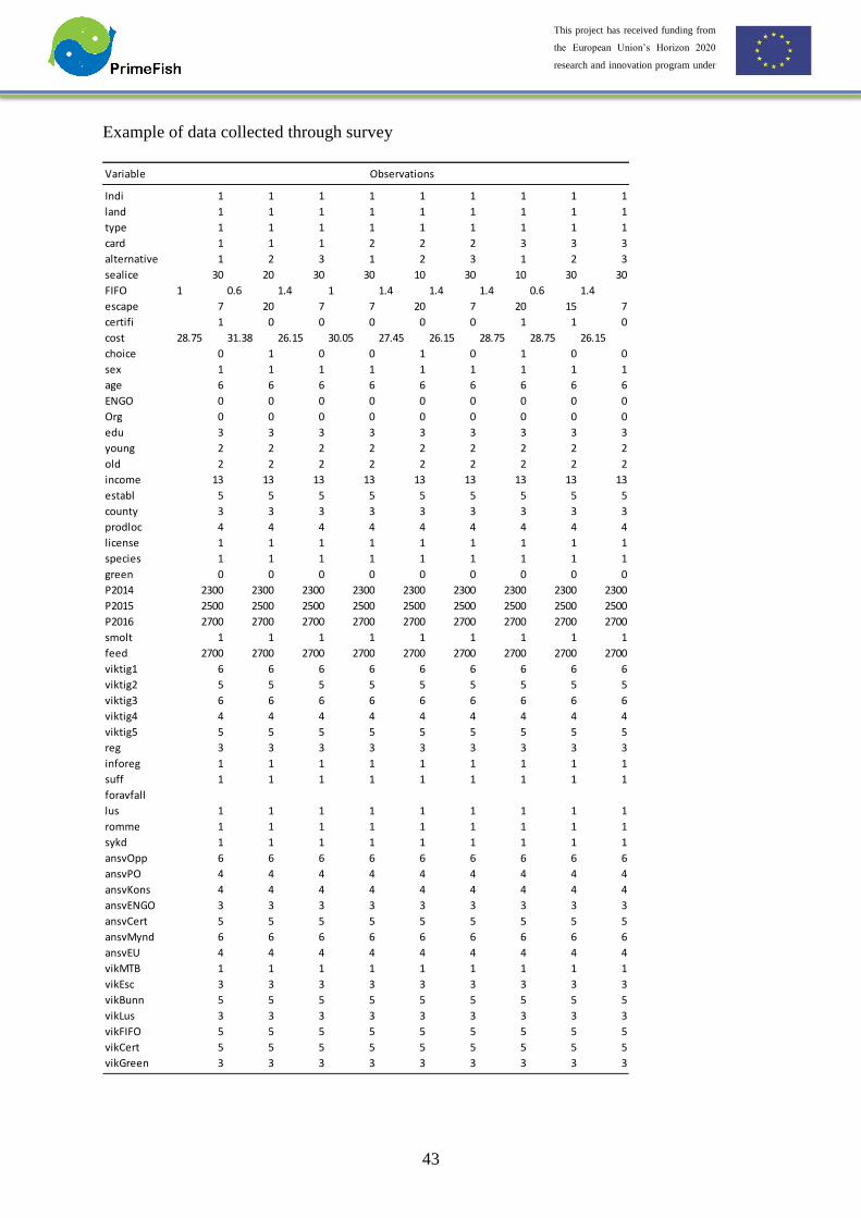
43





Example of data collected through survey

Variable

Indi 1 1 1 1 1 1 1 1 1

land 1 1 1 1 1 1 1 1 1

type 1 1 1 1 1 1 1 1 1

card 1 1 1 2 2 2 3 3 3

alternative 1 2 3 1 2 3 1 2 3

sealice 30 20 30 30 10 30 10 30 30

FIFO 1 0.6 1.4 1 1.4 1.4 1.4 0.6 1.4

escape 7 20 7 7 20 7 20 15 7

certifi 1 0 0 0 0 0 1 1 0

cost 28.75 31.38 26.15 30.05 27.45 26.15 28.75 28.75 26.15

choice 0 1 0 0 1 0 1 0 0

sex 1 1 1 1 1 1 1 1 1

age 6 6 6 6 6 6 6 6 6

ENGO 0 0 0 0 0 0 0 0 0

Org 0 0 0 0 0 0 0 0 0

edu 3 3 3 3 3 3 3 3 3

young 2 2 2 2 2 2 2 2 2

old 2 2 2 2 2 2 2 2 2

income 13 13 13 13 13 13 13 13 13

establ 5 5 5 5 5 5 5 5 5

county 3 3 3 3 3 3 3 3 3

prodloc 4 4 4 4 4 4 4 4 4

license 1 1 1 1 1 1 1 1 1

species 1 1 1 1 1 1 1 1 1

green 0 0 0 0 0 0 0 0 0

P2014 2300 2300 2300 2300 2300 2300 2300 2300 2300

P2015 2500 2500 2500 2500 2500 2500 2500 2500 2500

P2016 2700 2700 2700 2700 2700 2700 2700 2700 2700

smolt 1 1 1 1 1 1 1 1 1

feed 2700 2700 2700 2700 2700 2700 2700 2700 2700

viktig1 6 6 6 6 6 6 6 6 6

viktig2 5 5 5 5 5 5 5 5 5

viktig3 6 6 6 6 6 6 6 6 6

viktig4 4 4 4 4 4 4 4 4 4

viktig5 5 5 5 5 5 5 5 5 5

reg 3 3 3 3 3 3 3 3 3

inforeg 1 1 1 1 1 1 1 1 1

suff 1 1 1 1 1 1 1 1 1

foravfall

lus 1 1 1 1 1 1 1 1 1

romme 1 1 1 1 1 1 1 1 1

sykd 1 1 1 1 1 1 1 1 1

ansvOpp 6 6 6 6 6 6 6 6 6

ansvPO 4 4 4 4 4 4 4 4 4

ansvKons 4 4 4 4 4 4 4 4 4

ansvENGO 3 3 3 3 3 3 3 3 3

ansvCert 5 5 5 5 5 5 5 5 5

ansvMynd 6 6 6 6 6 6 6 6 6

ansvEU 4 4 4 4 4 4 4 4 4

vikMTB 1 1 1 1 1 1 1 1 1

vikEsc 3 3 3 3 3 3 3 3 3

vikBunn 5 5 5 5 5 5 5 5 5

vikLus 3 3 3 3 3 3 3 3 3

vikFIFO 5 5 5 5 5 5 5 5 5

vikCert 5 5 5 5 5 5 5 5 5

vikGreen 3 3 3 3 3 3 3 3 3

Observations

44





10 Analysis of European seafood products innovations

This section discussed the methodology used in deliverable 4.1 Industry study cases report: A

collection of marketing successes and failures in the world based on clever product innovations

and/or marketing activities.

To analyse the trend of sustainable seafood products in European markets, we look at the

evolution of the number of seafood products by categories of product (species, brand, claims…)

at the European level and then we focused on major species in the project: cod, herring, trout,

salmon, pangasius, seabass and seabream. Mostly descriptive statistics have been calculated

with mean comparison test (t-test) to ensure the statistical significance of trends and differences.

To have an accurate description of innovation trends in the European seafood market, we look

at trends in innovation between 2010 and 2015 across Europe. Nonetheless, we cannot be sure

that those trends are due to a real increase in seafood products innovation, as they could also be

caused by an extension in coverage of EU markets by Mintel. To solve this problem, we look

at the evolution of each classification of products in importance (by claims and type of launch).

Descriptive statistics and trend analyses were the most accurate methodologies in order to

analyse time series data. This is the standard methodology used for this type of analysis

The main strength of this approach is that by analysing the evolution of each classification of

products in importance, we avoid biases linked to data collection, and thus are able to analyse

real trends. The main weakness is that for some sub-categories the number of observations is

too low to reach definite conclusions.

45





11 Microeconomic demand analysis

This section reports the results of D4.3 entitled “Report on the development of fish consumption

and demand in France and Finland,” and D4.4, “Report on the impacts of increased fish

consumption on economic, health and environmental attributes” which are two of the

quantitative studies included in WP4 on “Products, consumers and seafood market trends.”

The economic theory of consumer choice provides the conceptual underpinning of the analysis.

Accordingly, consumers are assumed to choose the goods that they consume and their quantities

so as to maximize their well-being, or utility, subject to a budget constraint. Minimal

assumptions on preferences over combinations of goods are imposed to ensure the rationality

of choices. For instance, transitivity requires that if bundle A is strictly preferred to bundle B,

and bundle B to bundle C, then bundle A is also strictly preferred to bundle C. The budget

constraint arises because, for given levels of income and prices, only certain combinations of

goods (i.e., consumption bundles) can be afforded.

The main purpose of the analysis of demand is then to characterise consumer preferences from

observed consumption choices or, in other words, to let the data “reveal” preferences. This

differentiates the approach from the group of “stated preferences” methods that are also widely

used to investigate consumer behaviour, including in PrimeFish WP4. Both groups of methods

have their strengths and weaknesses, but in cases where markets exist, revealed preference

methods are usually considered superior because they do not suffer from the hypothetical biases

that plague stated preference methods (Murphy et al., 2005). On the other hand, revealed

preference methods are less suited to assess demand for a new product that is not currently

available to consumers, or to shed light on the cognitive and psychological processes underlying

choices.

In our framework, the theory guides the empirical inquiry first by identifying the variables that

should be legitimately included in the demand equations. Hence, the generic form of the

demand function for good i, denoted xi(p, m, z) takes several arguments:

● A vector of prices p, which means that demand for a good is a function of its own price,

but also the prices of substitute and complement goods.

● Income, or total expenditure, m, which defines the level of the budget constraint

● Socio-demographic variables z (e.g., education, age) that may be related in a systematic

way to consumer preferences.

46





At the estimation stage, the theory establishes criteria to compare specifications, reduces the

number of parameters to estimate, and ensures the realism of the simulations derived from the

model (e.g., adjustments of consumption to a price change remain compatible with the budget

constraint). In practice, three groups of restrictions follow from the axioms imposed on

consumer preferences (Deaton and Muellbauer, 1980): 1) Adding-up, which ensures that the

total value of demand exhausts the available budget; 2) Homogeneity, which imposes the

absence of money illusion (i.e., the fact that the same proportional increase in all prices and

total budget does not modify choices); and 3) Symmetry, which is less intuitive and relates to

the derivatives of the compensated demand functions. The fourth theoretical property of

negativity or concavity is usually not imposed but only checked expost.

The theoretical concepts of compensated (or Hicksian) demand and its difference with

uncompensated (or Marshallian) demand, are important to understand the model and interpret

its results. Marshallian demand denotes demand for a consumer operating under a budget

constraint, while Hicksian demand denotes demand for a consumer operating under a utility

constraint (i.e., holding his/her level of wellbeing constant). The first concept is of course closer

to reality, but understanding what happens when a price changes requires knowledge of the

second concept. For instance, assuming that the price of salmon increases, two different effects

determine the adjustment in Marshallian demand of a given household: first, the substitution

effect captures the reduction in consumption of salmon resulting from the fact that its price has

suddenly become higher relative to that of substitute goods (e.g., trout). Empirically, that

substitution effect is measured by the change in Hicksian demand, whose sign should be

unambiguously negative (i.e., demand for a good decreases with its own price). However, the

rise in the price of salmon also means that the real income/expenditure of the household has

decreased, or in other words that that consumer has become poorer. The change in Marshallian

demand also captures that second so-called income effect, and the above decomposition can

sometimes be useful to explain seemingly paradoxical results, as illustrated in the results

section.

The first step in the parametric estimation of demand relationships is the choice of a functional

form for the demand system, in order to allow imposition of the theoretical restrictions while

preserving flexibility (i.e., limit the restrictions on the system implicit in the functional form).

Several competing systems have been proposed, as reviewed by Barnett and Serlettis (2008)

47





with Deaton and Muelbauer’s Almost Ideal Demand System, or AIDS, remaining the most

popular one (Irz, 2010).

The AIDS model, however, presents two limiting features. First, it only allows income to

influence demand in a linear or log-linear form, when it is now well established that Engel

curves are often highly non-linear and vary widely in shapes across goods (Banks et al., 1997;

Lewbel, 1991). Second, the AIDS model does not allow for preference heterogeneity, which

unfortunately is recognized as a fundamental feature of consumer microdata (Crawford and

Pendakur, 2013), as indicated by the typically relatively poor fit of statistical models estimated

from such data.

As a way of addressing both issues, Lewbel and Pendakur (2009) have proposed the Exact

Affine Stone Index (EASI) demand system. The system’s Engel curves can be polynomials or

splines of any order in real expenditures and are therefore highly flexible. Further, the EASI

error terms equal random utility parameters, and the model therefore accounts for unobserved

preference heterogeneity in a theoretically consistent manner.

However, estimation of the model is complicated by endogeneity and non-linearity issues,

which means that iterative GMM or three-stage least squares procedures are called for. For

demand systems with censored data as specified in this study, it is likely that the computational

problems created by those procedures are insurmountable, and estimation of the full EASI

model was therefore deemed too challenging. Thus, we only estimate a simplified – or

approximate - version of the EASI model. Support for this simplification comes from Pendakur

(2009), who provides evidence that both linearity and endogeneity are only relatively small

issues in practice. In particular, that author finds that the linearized version of the model

estimated by Ordinary Least Squares (OLS) performs almost as well as fully-efficient

endogeneity-corrected nonlinear estimation.

Derivation of the EASI demand system starts from a dual representation of preferences in the

form of a minimum cost function:

where p is the J-vector of good prices; u denotes utility; z is a vector of observed socio-

economic characteristics (e.g., education); ε is a J-vector of unobserved preference

heterogeneity parameters; and mj (.) denotes an unrestricted function. Note that the specification

48





of parameters ajk as constants rather than a function of socio-demographic variables restricts

the influence of those variables on price responsiveness. By application of Shephard’s lemma,

we obtain the Hicksian cost share equations:

A few manipulations generate the implicit utility or real income y:

That manipulation represents the key step of the approach, as it permits to replace the

unobservable utility level u by y, which is solely a function of observables and parameters. The

implicit Marshallian budget shares then follow by substituting y, as expressed in equation (3),

for u in the Hicksian budget shares (2).

The advantages of the EASI model are evident in that expression. First, the functions mj(y, z)

are completely unrestricted in their dependence on implicit utility y and observable

demographic characteristics z. Thus, the model can accommodate homothetic preferences (i.e.,

independence of w from y), linear Engel curves as in the AIDS, quadratic Engel curves as in

the quadratic-AIDS model (QAIDS), or much more complex geometries of Engel curves.

Second, the unobserved preference heterogeneity parameters ε show up as error terms in the

estimated equations and as cost shifters in the cost function, and are thus an integral part of the

theoretical model.

We simplify the model further by assuming that the functions mj(.) are additively separable in

y and z, linear in z and polynomial of degree R in y:

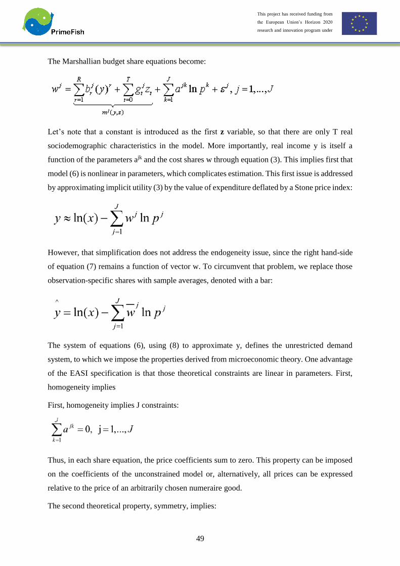
49





The Marshallian budget share equations become:

Let’s note that a constant is introduced as the first z variable, so that there are only T real

sociodemographic characteristics in the model. More importantly, real income y is itself a

function of the parameters ajk and the cost shares w through equation (3). This implies first that

model (6) is nonlinear in parameters, which complicates estimation. This first issue is addressed

by approximating implicit utility (3) by the value of expenditure deflated by a Stone price index:

However, that simplification does not address the endogeneity issue, since the right hand-side

of equation (7) remains a function of vector w. To circumvent that problem, we replace those

observation-specific shares with sample averages, denoted with a bar:

The system of equations (6), using (8) to approximate y, defines the unrestricted demand

system, to which we impose the properties derived from microeconomic theory. One advantage

of the EASI specification is that those theoretical constraints are linear in parameters. First,

homogeneity implies

First, homogeneity implies J constraints:

Thus, in each share equation, the price coefficients sum to zero. This property can be imposed

on the coefficients of the unconstrained model or, alternatively, all prices can be expressed

relative to the price of an arbitrarily chosen numeraire good.

The second theoretical property, symmetry, implies:

50





Hence, with J share equations (i.e., goods), there are J*(J-1)/2 such restrictions (i.e., the number

of non-diagonal elements of a J*J matrix divided by 2).

Finally, adding-up implies that the sum of the J coefficients associated with the constant of each

share equation (denoted z0) is equal to unity:

and the sum of the J coefficients associated with any other variable (i.e., price, socio-

demographic, or expenditure) is equal to zero:

Altogether, the model features JxJ price coefficients, Jx(T+1) socio-demographic coefficients

(including the constant terms), and JxR income coefficients, for a total of Jx(J+T+R+1). There

are J homogeneity constraints, Jx(J-1) /2 symmetry constraints, and R+J+T+1 adding-up

constraints, but it is easy to show that, for the price coefficients, imposing symmetry together

with any of the other two constraints implies that the third constraint is automatically satisfied.

Thus, there are only J(J+1)/2+R+T+1 independent constraints, and (J-1)(R+T+1+J/2)

independent coefficients to estimate.

The numerous parameters of the model are not interpretable directly, so that the next step in the

analysis is to compute elasticities. In general, the elasticity of any endogenous variable x with

respect to an exogenous variable p is defined as

.

This unitless quantity thus measures the responsiveness of x to p. The results section of this

report therefore presents the estimates of elasticities of demand with respect to prices, total

expenditure (i.e., budget), and sociodemographic variables.

The food choices that real-world consumers make involve thousands of products, which cannot

be modelled simultaneously within the framework of traditional demand theory. The usual

solution to this problem is to make a priori assumptions about consumers’ preferences and

51





decision making processes (Edgerton et al., 1996, p. 69). Here, the simplifying assumption is

that of multi-stage budgeting. Thus, it is assumed that, as depicted in Figure 1, the consumer’s

food budget is allocated in a first stage to broad categories of products, including an aggregate

of all fish and seafood products. In Stage 2, the fish budget is itself allocated to different

categories of fish products as defined by the type of processing method. For both countries,

those categories include fresh fish, smoked/marinated fish, canned fish and frozen fish, but the

French model also covers two additional categories: fish-based prepared dishes, as well as other

fish-based preparations (e.g., seafood spread). The third stage brings the analysis to the level of

the species.

At each stage, a demand system is estimated while holding total expenditure on the upper-level

aggregate constant. That is, the demand system for fresh fish estimates demand functions for

each species under the assumption that total expenditure on fresh fish remains constant, which

generates conditional elasticities (i.e., conditional on a constant fresh fish budget). Obviously

real consumers do not impose that sort of constraints upon themselves, so that in simulation

exercises, realism requires knowledge of unconditional elasticities, i.e. elasticities reflecting the

response of demand to a change when only total income (or expenditure, or the food budget) is

held constant. Carpentier and Guyomard (2003) have derived formulae to combine stage-

specific elasticities into unconditional elasticities, and the empirical section uses those formulas

to calculate unconditional elasticities.

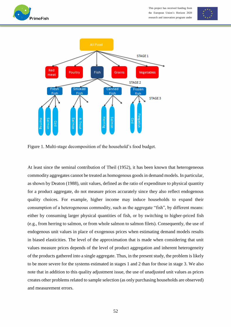
52





Figure 1. Multi-stage decomposition of the household’s food budget.

At least since the seminal contribution of Theil (1952), it has been known that heterogeneous

commodity aggregates cannot be treated as homogenous goods in demand models. In particular,

as shown by Deaton (1988), unit values, defined as the ratio of expenditure to physical quantity

for a product aggregate, do not measure prices accurately since they also reflect endogenous

quality choices. For example, higher income may induce households to expand their

consumption of a heterogeneous commodity, such as the aggregate “fish”, by different means:

either by consuming larger physical quantities of fish, or by switching to higher-priced fish

(e.g., from herring to salmon, or from whole salmon to salmon filets). Consequently, the use of

endogenous unit values in place of exogenous prices when estimating demand models results

in biased elasticities. The level of the approximation that is made when considering that unit

values measure prices depends of the level of product aggregation and inherent heterogeneity

of the products gathered into a single aggregate. Thus, in the present study, the problem is likely

to be more severe for the systems estimated in stages 1 and 2 than for those in stage 3. We also

note that in addition to this quality adjustment issue, the use of unadjusted unit values as prices

creates other problems related to sample selection (as only purchasing households are observed)

and measurement errors.

53





Fortunately, the literature on the subject offers several options to correct unit values to make it

possible to use them as price variables, as reviewed partially in Aepli (2014). Cox and

Wohlgenant (1986) paved the way by showing how regressions of unit values on variables

thought to influence quality choices (e.g., household size, education) can be used to “clean”

unit values of their quality component. Their method, which is very close to that subsequently

proposed by Park and Capps (1997), remains widely used in microeconometric analysis of

household consumption. Based on the theoretical model of quantity versus quality choice of

Houthakker (1952), a unit value equation is specified as relating the unit value to: 1- Forces

with a strong influence on supply conditions (hence prices), which are of particular importance

in order to identify demand relationships. Typically, regional, seasonal and, where appropriate,

yearly dummies are included, or the unit value equation are expressed in terms of deviation

from regional/seasonal/annual means; and 2- Variables thought to influence quality choices,

such as household size, or income. More recent developments of the approach also include the

physical amount of the category aggregate to accommodate the possibility that the same goods

purchased in larger quantities entail lower unit values. In a second stage, adjusted prices are

calculated by removing from unit values the estimated effect of all the variables in the second

group (i.e., influencing quality choices) or, equivalently, by adding the household-specific

residual to the estimated effect of the first group of variables. Given that residuals are not

available for non-consuming households, they are simply assumed to be zero so as to allow

estimation of demand relationships over the whole sample. The empirical analysis presented

below used the Park and Capps (1997) approach to correct unit values.

The high prevalence of zero consumption observations in microeconomic data sets used to

estimate demand systems is very common (Coelho et al., 2010). The fundamental problem that

this creates results from the fact that an observation of zero consumption may not indicate that

the household does not and will never consume the food concerned, since other possibilities are

equally plausible. Zero consumption may be attributable to the infrequency of purchase of some

food items, although this is less likely when consumption is recorded over a long period of time,

as is the case with consumer panels. In addition to infrequency of purchase, an observation of

zero consumption can also reflect a corner solution to the utility maximization problem: given

its current income and prevailing prices, the household does not purchase the food item.

However, under different economic circumstances, the household may opt to consume the good

(Maddala, 1983).

54





Zero consumption explained by infrequency of purchase or corner solutions implies that the

dependent variable, consumption, is censored, which creates an econometric problem

particularly difficult to address in the case of multivariate models, such as demand systems.

Ignoring censoring by treating zero values as any other value of the consumption variable

produces estimates of demand models, and elasticities, which are known to be both biased and

inconsistent. The most complete treatment of this issue considers the simultaneous estimation

of the decision to consume each good (i.e., a binary problem) and the decision regarding the

amount of the good that should be purchased. However, when a system of multiple equations

is considered, direct estimation involves the resolution of multiple integrals in the likelihood

functions, which proves computationally intensive and often intractable.

Thus, more tractable multi-stage estimation procedures of censored demand models have been

developed. Heien and Wessels (1990) (henceforth HS) used the general Heckman procedure to

propose an estimation in two simple steps. In the first step, a probit equation is estimated to

model the binary decision to consume a food item and, in a second step, the demand equations

are augmented by the inverse mills ratios extracted from the first-step regressions. Shonkwiler

and Yen (1999) (henceforth SY), however, have demonstrated the inconsistency of the HS

estimator before offering a consistent alternative. That procedure is still widely used in

empirical demand analysis (e.g., Gustavsen and Rickertsen, 2014) and we adopt it as it

represents a good compromise between theoretical soundness and empirical tractability. In a

first step, as in the HS framework, the probabilities of consuming positive quantities of any

given food item are estimated by probit models. The terms related to the first-stage probit

equations are then introduced to correct the bias in the coefficients of the EASI model brought

about by censoring. Thus, those corrected coefficients can be used as such in the expressions

of the elasticities previously described.

The microeconomic analysis of demand for fish in D4.3 and D4.4 was carried out using the

methodology presented above. The method proceeds in several steps:

• Descriptive statistics are used to characterize the market of interest and its evolution.

This generates background and hypotheses but is insufficient to pinpoint the exact

drivers of demand.

• Based on the economic theory of consumer choice, demand functions for different

seafood products are derived, and the links among demand functions are made

explicit. This allows one to specify three types of observables that influence

55





consumers’ decisions to purchase fish, namely prices, income and socio-demographics

related to tastes and preferences.

• A functional form is imposed to define empirically estimable demand relationships. In

our case the approximate Exact Affine Stone Index (EASI) demand system was

chosen because of its flexibility.

• The demand relationships are estimated as a system through appropriate econometric

procedures.

The results of that analysis are summarized by elasticities measuring the response of demand

to exogenous changes in the economic environment (prices, income) as well as the extent to

which demand depends on socio-demographic variables. However, we developed the analysis

further to produce simulations that make it easier to communicate the results effectively to non-

specialists.

At a broad level, the method uses actual market transaction data (i.e., real purchases made by

real consumers) to characterise consumers’ preferences for fish. In other words, it lets the data

“reveal” preferences. This differentiates the approach from the group of “stated preferences”

methods that are also widely used to investigate consumer behaviour, including in PrimeFish

WP4, and rely on consumers’ statements about hypothetical situations. Both groups of methods

have their strengths and weaknesses, but in cases where markets exist, revealed preference

methods are usually considered superior because they do not suffer from the hypothetical biases

that plague stated preference methods. On the other hand, revealed preference methods are less

suited to assess demand for a new product that is not currently available to consumers, or to

shed light on the cognitive and psychological processes underlying choices.

We used the most common method used to analyse the structure of demand in seafood markets,

as stated for instance in this publication:

However, as mentioned above, stated preference methods can be used to analyse determinants

of demand as well. Within the group of revealed preference methods, alternative approaches

(e.g., random utility model) are available but they are more appropriate to investigate demand

for highly differentiated products (e.g., different brands).

The main strength of the methodology applied is to rely on observations of what consumers

actually do rather than what they say they will do. However, relying on secondary data has its

drawbacks. First, the data are expensive to purchase. Second, some variables of interest, for

56





instance regarding consumers’ motivations to purchase fish, values and health status, are not

measured in those data sets. Finally, the results are sometimes sensitive to the choice of

estimation method.

The approach relies on very detailed data, i.e., “Big Data”, which makes the analysis rather

involved, technical and time consuming. While convenient tools exist to visualize and describe

that type of data, going further to carry a full demand analysis remains difficult and requires

specialist skills. However, tools may be developed in the future to limit the obstacles to that

type of analysis.

.

57





12 Frequency of purchases

The purpose of deliverable 4.5 report on frequencies of consumer purchases is to analyse what

determines how frequently consumers buy seafood products. The methodology used is based

on a system of demand equations, in terms of purchase frequencies, using a negative binomial

model which is a modified version of the microeconomic model by Meghir and Robin (1992).

In particular, the aim is to determine what types of consumers purchase the following seafood

product categories; fresh salmon, frozen salmonids (salmon and trout), fresh cod, frozen white

fish (cod, haddock, saithe etc.) and all other seafood products.

We approach the problem from the angle of purchasing frequencies, that is, how often

households purchase various types of fish. The object is to combine aspects from the marketing

literature and the economic demand literature, which have analysed consumer behavior from

different angles, to utilise the strengths of both approaches in order to produce valuable

information for those who wish to sell fish in France.

Conventional demand analysis aims at understanding markets by predicting consumption and

understanding how demand relates to prices, expenditure, and socioeconomic variables.

Various studies of the demand for fish exist in the literature. Thus, Asche et al. (2011) analyse

demand for Atlantic salmon in the EU, especially France. Gobillon and Wolff (2015)

investigate spatial variations in product prices in French fish markets, while Onozaka et al.

(2014) analyse the relationship between consumer perception and salmon consumption

frequencies. Xie and Myrland (2011) apply an empirical test for the aggregation levels of

French household demand for salmon. The marketing literature has focused more on count data

models which have been widely applied for different purposes, such as evaluating brand

success, brand loyalty, and store choice. Kau and Ehrenberg (1984) use the negative binomial

(NB) Dirichlet4 model to predict store choice. Uncles et al. (1995) is a review paper on buyer

regularities based on predictions from the NB Dirchlet model. Bhattacharya (1997) estimates

deviations from brand loyalty and compares it with predictions from the Dirchlet model, and

4 The negative binomial Dirichlet model has two stages; the first is a form of the multivariate beta distribution

known as the Dirichlet distribution, and the second is a Poisson gamma mixture which produces a variant of the

negative binomial model. The Dirichlet is assumed to be the data generating process (DGP) of some choice and

the negative binomial is assumed to be the DGP of the frequency of the corresponding choice.

58





Uncles and Lee (2006) estimate the purchase frequency of different age groups using

predictions from the NB Dirichlet model.5

A specific branch of the demand literature has applied count data models in demand analysis,

where the key references are Meghir and Robin (1992) and Robin (1993). However, these

studies do not use count data estimation as their main focus, but rather employ the estimated

probabilities to adjust conventional demand models to account for the actual purchase

frequency of consumers, instead of utilising only the observed choice to purchase or not. In

general, though, the economics literature has only applied count data models to a very restricted

set of problems, e.g. the estimation of recreational demand and demand for health care. The

standard count data models are the Poisson and the negative binomial, where the negative

binomial is a natural extension to the Poisson which allows for a variance which differs from

the mean. The Poisson and negative binomial have been applied, for example, by Creel and

Loomis (1990), and Hellerstein (19991) to estimate recreational demand. Munkin and Trivedi

(1999), Deb and Trivedi (2002), and Wang (2003) estimate the demand for health care.

Consider a consumer that faces the following optimisation problem

max𝑙,𝑐,𝑛

{𝑈(𝑙, 𝑐, 𝑛): 𝑤𝑇 + 𝑅 = 𝑝′𝑐 + 𝑤𝑙 + 𝑤𝐿(𝑛), 𝑙 > 0, 𝑐 > 0, 𝑛 > 0} (1)

where U denotes utility, l leisure, 𝑐 = (𝑐1, 𝑐2, … , 𝑐𝑀)′ is a vector of consumption goods and

𝑛 = (𝑛1, 𝑛2, … , 𝑛𝑀)′ represents the corresponding purchase frequency. We assume that the

consumer’s utility function, 𝑢(𝑙, 𝑐, 𝑛), is weakly separable and quasi-concave in l, c, and n. The

consumer has income 𝑦 = 𝑤ℎ, where h is the hours spent working and w is the hourly wage

rate, as well as other income through transfers and undeclared activities, R. Total available time

is T, which is split into total hours worked h, time spent purchasing goods which is given by

the function 𝐿(𝑛), which is increasing in n, and other non-market hours, l. From the

aforementioned assumptions, the consumer’s optimization problem can be expressed as

follows:

max𝑙,𝑐,𝑛

{𝑢(𝑙, 𝑐, 𝑛): 𝑤𝑇 + 𝑅 = 𝑝′𝑐 + 𝑤𝑙 + 𝑤𝐿(𝑛), 𝑙 > 0, 𝑐 > 0, 𝑛 > 0} (1)

5 The Dirichlet distribution is generally not used in economics, but one example is Shonkwiler and Englin (2005)

who use it to estimate the willingness to pay for removing grazing land from hiking trails.

59





The solution to the optimization problem are three sets of Marshallian demand equations,

𝑙(𝑝, 𝑤, 𝑅), 𝑛𝑖(𝑝, 𝑤, 𝑅), and 𝑐𝑖(𝑝, 𝑤, 𝑅), where 𝑖 = 1,2, … , 𝑀. This deliverable, however, only

focuses on the purchase frequency decision. Let the number of shopping trips be generated by

a discrete distribution with a probability mass function 𝑓𝑁(𝑛|𝑍𝑖) for 𝑛 = 0,1,2, … where 𝑍𝑖 is a

matrix of exogenous variables, then the probability of observing 𝑛 = 0 is given by

Pr(𝑁 = 0|𝑍𝑖).

To be able to estimate the model it is necessary to specify the probability mass function of n.

The usual starting point of count data estimation is to assume the Poisson distribution, which

was used in Meghir and Robin (1992) to estimate their system of purchase frequency demand.

This is a valid choice since quasi-maximum likelihood will lead to an unbiased estimation even

though the distribution assumptions are incorrect as long as the mean is correctly specified.

However, due to the Poisson limitations of equidispersion we assume instead the negative

binomial distribution:

𝑓(𝑛𝑖|𝑍𝑖) =Γ(𝜃 + 𝑛𝑖)𝑟𝜃(1 − 𝑟)𝑛𝑖

Γ(1 + 𝑛𝑖)Γ(𝜃), 𝑟 =

𝜃

𝜃 + 𝜆, 0,1,2, …

(2)

The conditional mean of 𝑛𝑖 is then E(𝑛𝑖|𝑍𝑖) = 𝜆𝑖 and the conditional variance is V(𝑛𝑖|𝑍𝑖) =

𝜆 (1 +1

𝜃𝜆) = 𝜆(1 + 𝜅𝜆) = (𝜆 + 𝜅𝜆2). This specification of the negative binomial model is

known as the NB2, due to the square of the lambda parameter in the variance specification.6 As

in Meghir and Robin (1992) no stochastic relationship is assumed between different E(𝑛𝑖|𝑍𝑖) =

𝜆𝑖. To be able to estimate a count data system with a dimension greater than two or three and

an unrestricted covariance matrix one must use simulation based methods, see for example Chib

and Winkelmann (2001).

The method chosen for this analysis represents state-of-the-art methodology. The models used

are modified – and hopefully improved – version of the models proposed by Meghir and Robin

(1992) and Robin (1993).

This is the standard methodology used in the field, but other, less statistically advanced,

methods can certainly be employed to illustrate frequencies of purchases.

The method is typically used on consumer data such as scanner data which show “true”

consumer behaviour as reflected by their purchases of goods and services. This yields a better

6 See Cameron and Trivedi (2013) for details.

60





picture of how consumers behave than surveys. However, the datasets – just like surveys – do

not include all the variables researchers might be interested in using in their surveys. The

models employed are based on classical microeconomic theory which has been criticised for its

rather stringent assumption about homo economicus. The results of the methods are often

sensitive to the choice of the estimation method and the restrictions imposed by theory. Finally,

consumer data can be expensive to purchase.

The aim is to understand consumer behaviour in the French fish market using a frequency of

purchase approach, which is significantly different from the standard demand system studies in

the economics literature. The frequency of purchase approach, as we present it, models how

often consumers purchase from each category of fish, as specified in the paper, and not how

much quantity is purchased, or how much is spent in Euros on each category as is so often done

in standard demand analysis. The strength of the frequency of purchase approach stems from

the fact that purchasing behaviour is mainly determined by how often one purchases goods and

not how much is purchased on each occasion. Furthermore, the results from the model show

how prices, expenditure and socioeconomic variables relate to purchase frequencies, which then

enables companies to construct their pricing strategy in such a way that each consumer

purchases as frequently as possible. If the firm is a supermarket, which has a wide selection of

products, and has fish on sale then customers who come to the supermarket with the aim of

purchasing cheap fish are likely to purchase a range of other products as well, due to the

opportunity cost of time.

The frequency of purchase approach, as we present it, has the flaw of not accounting for average

purchased quantity. Even though the information that this addition would bring might be limited

it would still improve the strength of the estimation. In comparison with the standard estimation

framework where average quantity purchased and frequencies is lumped together in a variable

such as total purchased quantity, expenditures on each category, or budget shares information

is still lost, since frequencies of purchase are not modelled specifically. The two approaches

both have their pros and cons and the choice of which model to use depends highly upon the

problem at hand.

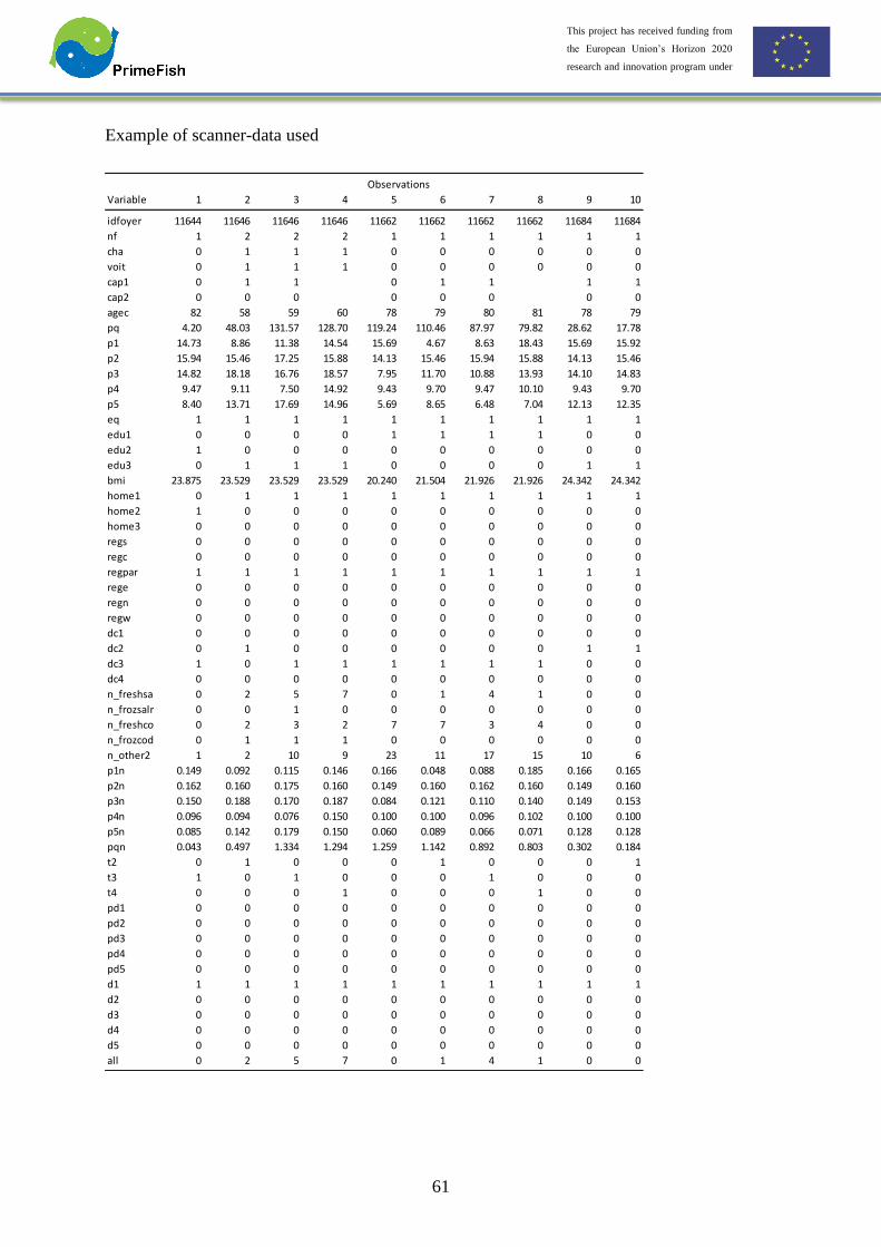
61





Example of scanner-data used

Variable 1 2 3 4 5 6 7 8 9 10

idfoyer 11644 11646 11646 11646 11662 11662 11662 11662 11684 11684

nf 1 2 2 2 1 1 1 1 1 1

cha 0 1 1 1 0 0 0 0 0 0

voit 0 1 1 1 0 0 0 0 0 0

cap1 0 1 1 0 1 1 1 1

cap2 0 0 0 0 0 0 0 0

agec 82 58 59 60 78 79 80 81 78 79

pq 4.20 48.03 131.57 128.70 119.24 110.46 87.97 79.82 28.62 17.78

p1 14.73 8.86 11.38 14.54 15.69 4.67 8.63 18.43 15.69 15.92

p2 15.94 15.46 17.25 15.88 14.13 15.46 15.94 15.88 14.13 15.46

p3 14.82 18.18 16.76 18.57 7.95 11.70 10.88 13.93 14.10 14.83

p4 9.47 9.11 7.50 14.92 9.43 9.70 9.47 10.10 9.43 9.70

p5 8.40 13.71 17.69 14.96 5.69 8.65 6.48 7.04 12.13 12.35

eq 1 1 1 1 1 1 1 1 1 1

edu1 0 0 0 0 1 1 1 1 0 0

edu2 1 0 0 0 0 0 0 0 0 0

edu3 0 1 1 1 0 0 0 0 1 1

bmi 23.875 23.529 23.529 23.529 20.240 21.504 21.926 21.926 24.342 24.342

home1 0 1 1 1 1 1 1 1 1 1

home2 1 0 0 0 0 0 0 0 0 0

home3 0 0 0 0 0 0 0 0 0 0

regs 0 0 0 0 0 0 0 0 0 0

regc 0 0 0 0 0 0 0 0 0 0

regpar 1 1 1 1 1 1 1 1 1 1

rege 0 0 0 0 0 0 0 0 0 0

regn 0 0 0 0 0 0 0 0 0 0

regw 0 0 0 0 0 0 0 0 0 0

dc1 0 0 0 0 0 0 0 0 0 0

dc2 0 1 0 0 0 0 0 0 1 1

dc3 1 0 1 1 1 1 1 1 0 0

dc4 0 0 0 0 0 0 0 0 0 0

n_freshsalm2 0 2 5 7 0 1 4 1 0 0

n_frozsalm2 0 0 1 0 0 0 0 0 0 0

n_freshcod2 0 2 3 2 7 7 3 4 0 0

n_frozcod2 0 1 1 1 0 0 0 0 0 0

n_other2 1 2 10 9 23 11 17 15 10 6

p1n 0.149 0.092 0.115 0.146 0.166 0.048 0.088 0.185 0.166 0.165

p2n 0.162 0.160 0.175 0.160 0.149 0.160 0.162 0.160 0.149 0.160

p3n 0.150 0.188 0.170 0.187 0.084 0.121 0.110 0.140 0.149 0.153

p4n 0.096 0.094 0.076 0.150 0.100 0.100 0.096 0.102 0.100 0.100

p5n 0.085 0.142 0.179 0.150 0.060 0.089 0.066 0.071 0.128 0.128

pqn 0.043 0.497 1.334 1.294 1.259 1.142 0.892 0.803 0.302 0.184

t2 0 1 0 0 0 1 0 0 0 1

t3 1 0 1 0 0 0 1 0 0 0

t4 0 0 0 1 0 0 0 1 0 0

pd1 0 0 0 0 0 0 0 0 0 0

pd2 0 0 0 0 0 0 0 0 0 0

pd3 0 0 0 0 0 0 0 0 0 0

pd4 0 0 0 0 0 0 0 0 0 0

pd5 0 0 0 0 0 0 0 0 0 0

d1 1 1 1 1 1 1 1 1 1 1

d2 0 0 0 0 0 0 0 0 0 0

d3 0 0 0 0 0 0 0 0 0 0

d4 0 0 0 0 0 0 0 0 0 0

d5 0 0 0 0 0 0 0 0 0 0

all 0 2 5 7 0 1 4 1 0 0

Observations

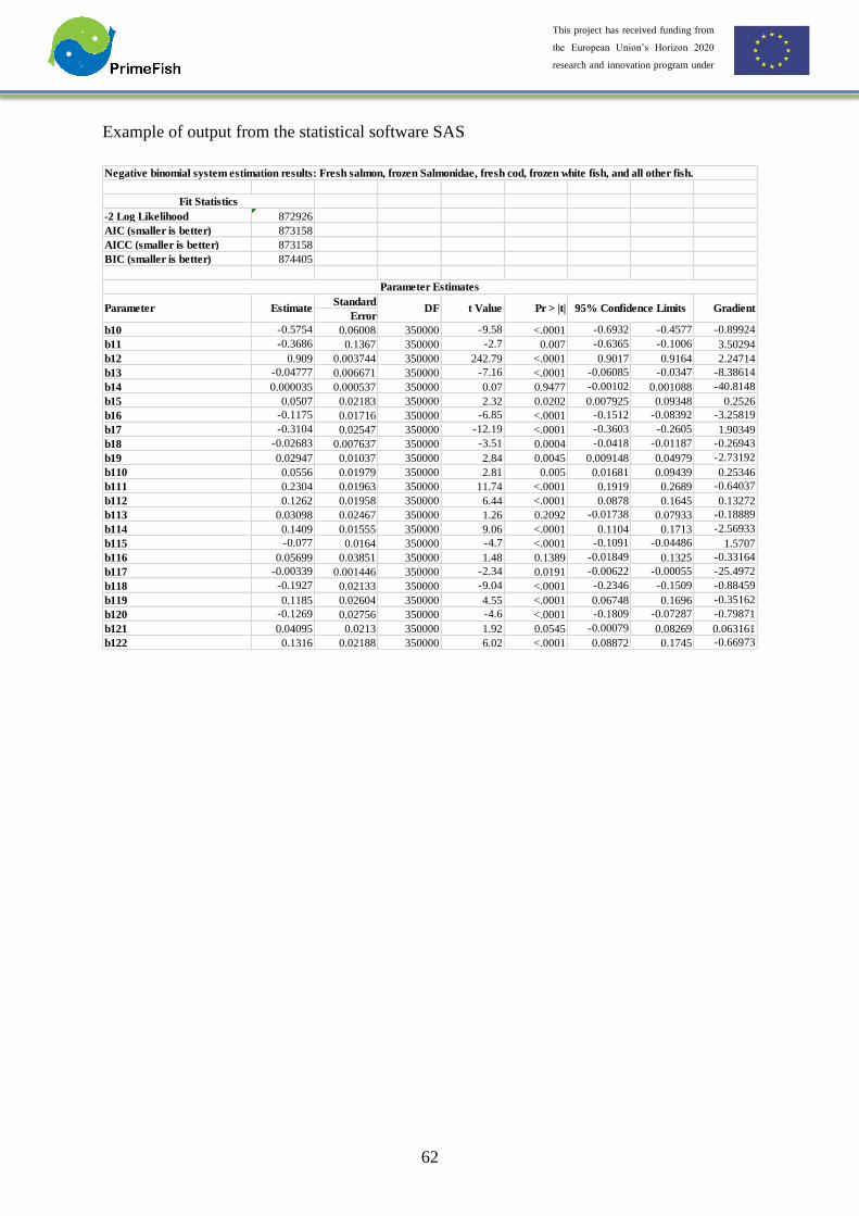
62





Example of output from the statistical software SAS

Negative binomial system estimation results: Fresh salmon, frozen Salmonidae, fresh cod, frozen white fish, and all other fish.

-2 Log Likelihood 872926

AIC (smaller is better) 873158

AICC (smaller is better) 873158

BIC (smaller is better) 874405

Standard

Error

b10 -0.5754 0.06008 350000 -9.58 <.0001 -0.6932 -0.4577 -0.89924

b11 -0.3686 0.1367 350000 -2.7 0.007 -0.6365 -0.1006 3.50294

b12 0.909 0.003744 350000 242.79 <.0001 0.9017 0.9164 2.24714

b13 -0.04777 0.006671 350000 -7.16 <.0001 -0.06085 -0.0347 -8.38614

b14 0.000035 0.000537 350000 0.07 0.9477 -0.00102 0.001088 -40.8148

b15 0.0507 0.02183 350000 2.32 0.0202 0.007925 0.09348 0.2526

b16 -0.1175 0.01716 350000 -6.85 <.0001 -0.1512 -0.08392 -3.25819

b17 -0.3104 0.02547 350000 -12.19 <.0001 -0.3603 -0.2605 1.90349

b18 -0.02683 0.007637 350000 -3.51 0.0004 -0.0418 -0.01187 -0.26943

b19 0.02947 0.01037 350000 2.84 0.0045 0.009148 0.04979 -2.73192

b110 0.0556 0.01979 350000 2.81 0.005 0.01681 0.09439 0.25346

b111 0.2304 0.01963 350000 11.74 <.0001 0.1919 0.2689 -0.64037

b112 0.1262 0.01958 350000 6.44 <.0001 0.0878 0.1645 0.13272

b113 0.03098 0.02467 350000 1.26 0.2092 -0.01738 0.07933 -0.18889

b114 0.1409 0.01555 350000 9.06 <.0001 0.1104 0.1713 -2.56933

b115 -0.077 0.0164 350000 -4.7 <.0001 -0.1091 -0.04486 1.5707

b116 0.05699 0.03851 350000 1.48 0.1389 -0.01849 0.1325 -0.33164

b117 -0.00339 0.001446 350000 -2.34 0.0191 -0.00622 -0.00055 -25.4972

b118 -0.1927 0.02133 350000 -9.04 <.0001 -0.2346 -0.1509 -0.88459

b119 0.1185 0.02604 350000 4.55 <.0001 0.06748 0.1696 -0.35162

b120 -0.1269 0.02756 350000 -4.6 <.0001 -0.1809 -0.07287 -0.79871

b121 0.04095 0.0213 350000 1.92 0.0545 -0.00079 0.08269 0.063161

b122 0.1316 0.02188 350000 6.02 <.0001 0.08872 0.1745 -0.66973

Fit Statistics

Parameter Estimates

Parameter Estimate DF t Value Pr > |t| 95% Confidence Limits Gradient

63





13 Analysis of social awareness

This section discusses the methodology applied in deliverable 4.6 Report on social awareness,

attempts to stimulate fish consumption, and negative press.

The quantitative data was mainly analysed using different types of bivariate and multivariate

data analysis. The purpose of these types of analysis is to determine the empirical relationship

between two or several variables. The qualitative data is mainly based on literature review, but

it also contains qualitative responses collected through questionnaire. The qualitative answers

were analysed based on coding and qualitative comparative analysis.

These methodologies were used because they are simple to implement and because they

correspond to the type of collected data. The bivariate and multivariate data analysis permitted

to test the simple hypotheses of associations, especially between socio-demographic variables

and fish consumption variables. Bivariate analysis was also used to analyse the impact of type

of negative information on variables such as attitudes and intentions.

This type of analysis is a standard methodology used in the field. Another option could be

structural equation model, that will be applied later in the scientific papers based on this data

set.

The applied methodologies are simple to apply and robust. The weakness of the used methods,

compared to structural equation model is the fact that it doesn’t permit a fine analysis of latent

variables.

The data didn’t limit the choice of methodology, but on the basis of our experiment it might be

better to base the analysis on both quantitative and qualitative data and to do statistical tests to

check the quality of results. Furthermore, better analysis of latent variables (in our case:

involvement, health sensitiveness and environmental sensitiveness) could be obtained by

employing structural equation models.

64





14 Choice experiments

This section discusses the methodology employed for deliverable 4.7 Choice modelling report

on innovative features and the consumers’ willingness to pay.

According to Lancaster’s consumer theory (1966), consumer utility stems from product

attributes, not the products themselves. In other words, consumer utility can be separated into

part-worth utilities. The part-worth utilities equal consumers’ preference for corresponding

attributes. In marketing research, the product attributes are classified into extrinsic and intrinsic

attributes (Zeithaml, 1988; Olsen et al., 2008). Regardless of whether consumers are exposed

to these attributes, they may be important signals of product quality and determinants of

consumer preference.

The overall utility that a consumer obtains from consuming a seafood species j (Uj) can be

expressed as:

𝑢𝑖𝑗 = 𝑥𝑖𝑗′ 𝛽 + 휀𝑖𝑗 (1)

where: i=1,….N: Individual consumer i,

j=1,….J: product j among J products,

𝑢𝑖𝑗: utility obtained by individual i from product j,

𝑥𝑖𝑗′ : product attributes,

β: vector of part-worth utility,

휀𝑖𝑗: random effect.

It is generally assumed that an individual would choose a product alternative if the utility

derived from this alternative is maximized compared to the other alternatives:

𝑦𝑖𝑗 = {1, 𝑖𝑓 𝑢𝑖𝑗 ≥ max (𝑢𝑖)

0 𝑜𝑡ℎ𝑒𝑟𝑤𝑖𝑠𝑒 (2)

When facing a “basket” of seafood products, consumers assign a random utility to each product

alternatives and select the one with the highest derived utility. Assuming that the stochastic

components 휀𝑗 have independent and identical distributed (iid) forms, the probability of a

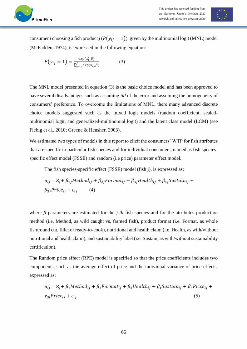
65





consumer i choosing a fish product j (𝑃(𝑦𝑖𝑗 = 1)) given by the multinomial logit (MNL) model

(McFadden, 1974), is expressed in the following equation:

𝑃(𝑦𝑖𝑗 = 1) =exp (𝑥𝑖𝑗

′ 𝛽)

∑ exp (𝑥𝑖𝑘′ 𝛽)

𝐽𝑘=1

(3)

The MNL model presented in equation (3) is the basic choice model and has been approved to

have several disadvantages such as assuming iid of the error and assuming the homogeneity of

consumers’ preference. To overcome the limitations of MNL, there many advanced discrete

choice models suggested such as the mixed logit models (random coefficient, scaled-

multinomial logit, and generalized-multinomial logit) and the latent class model (LCM) (see

Fiebig et al., 2010; Greene & Hensher, 2003).

We estimated two types of models in this report to elicit the consumers’ WTP for fish attributes

that are specific to particular fish species and for individual consumers, named as fish species-

specific effect model (FSSE) and random (i.e price) parameter effect model.

The fish species-specific effect (FSSE) model (fish j), is expressed as:

𝑢𝑖𝑗 =∝𝑗+ 𝛽1𝑗𝑀𝑒𝑡ℎ𝑜𝑑𝑖𝑗 + 𝛽2𝑗𝐹𝑜𝑟𝑚𝑎𝑡𝑖𝑗 + 𝛽3𝑗𝐻𝑒𝑎𝑙𝑡ℎ𝑖𝑗 + 𝛽4𝑗𝑆𝑢𝑠𝑡𝑎𝑖𝑛𝑖𝑗 +

𝛽5𝑗𝑃𝑟𝑖𝑐𝑒𝑖𝑗 + 휀𝑖𝑗 (4)

where β parameters are estimated for the j-th fish species and for the attributes production

method (i.e. Method, as wild caught vs. farmed fish), product format (i.e. Format, as whole

fish/round cut, fillet or ready-to-cook), nutritional and health claim (i.e. Health, as with/without

nutritional and health claim), and sustainability label (i.e. Sustain, as with/without sustainability

certification).

The Random price effect (RPE) model is specified so that the price coefficients includes two

components, such as the average effect of price and the individual variance of price effects,

expressed as:

𝑢𝑖𝑗 =∝𝑗+ 𝛽1𝑀𝑒𝑡ℎ𝑜𝑑𝑖𝑗 + 𝛽2𝐹𝑜𝑟𝑚𝑎𝑡𝑖𝑗 + 𝛽3𝐻𝑒𝑎𝑙𝑡ℎ𝑖𝑗 + 𝛽4𝑆𝑢𝑠𝑡𝑎𝑖𝑛𝑖𝑗 + 𝛽5𝑃𝑟𝑖𝑐𝑒𝑖𝑗 +

𝛾3𝑖𝑃𝑟𝑖𝑐𝑒𝑖𝑗 + 휀𝑖𝑗 (5)

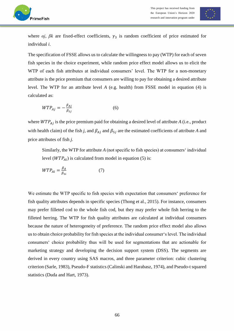
66





where αj, βk are fixed-effect coefficients, 𝛾3 is random coefficient of price estimated for

individual i.

The specification of FSSE allows us to calculate the willingness to pay (WTP) for each of seven

fish species in the choice experiment, while random price effect model allows us to elicit the

WTP of each fish attributes at individual consumers’ level. The WTP for a non-monetary

attribute is the price premium that consumers are willing to pay for obtaining a desired attribute

level. The WTP for an attribute level A (e.g. health) from FSSE model in equation (4) is

calculated as:

𝑊𝑇𝑃𝐴𝑗 = −𝛽𝐴𝑗

𝛽5𝑗 (6)

where 𝑊𝑇𝑃𝐴𝑗 is the price premium paid for obtaining a desired level of attribute A (i.e., product

with health claim) of the fish j, and 𝛽𝐴𝑗 and 𝛽5𝑗 are the estimated coefficients of attribute A and

price attributes of fish j.

Similarly, the WTP for attribute A (not specific to fish species) at consumers‘ individual

level (𝑊𝑇𝑃𝐴𝑖) is calculated from model in equation (5) is:

𝑊𝑇𝑃𝐴𝑖 =𝛽𝐴

𝛽5𝑖 (7)

We estimate the WTP specific to fish species with expectation that consumers‘ preference for

fish quality attributes depends in specific species (Thong et al., 2015). For instance, consumers

may prefer filleted cod to the whole fish cod, but they may prefer whole fish herring to the

filleted herring. The WTP for fish quality attributes are calculated at individual consumers

because the nature of heterogeneity of preference. The random price effect model also allows

us to obtain choice probability for fish species at the individual consumer‘s level. The individual

consumers‘ choice probability thus will be used for segmentations that are actionable for

marketing strategy and developing the decision support system (DSS). The segments are

derived in every country using SAS macros, and three parameter criterion: cubic clustering

criterion (Sarle, 1983), Pseudo-F statistics (Calinski and Harabasz, 1974), and Pseudo-t squared

statistics (Duda and Hart, 1973).

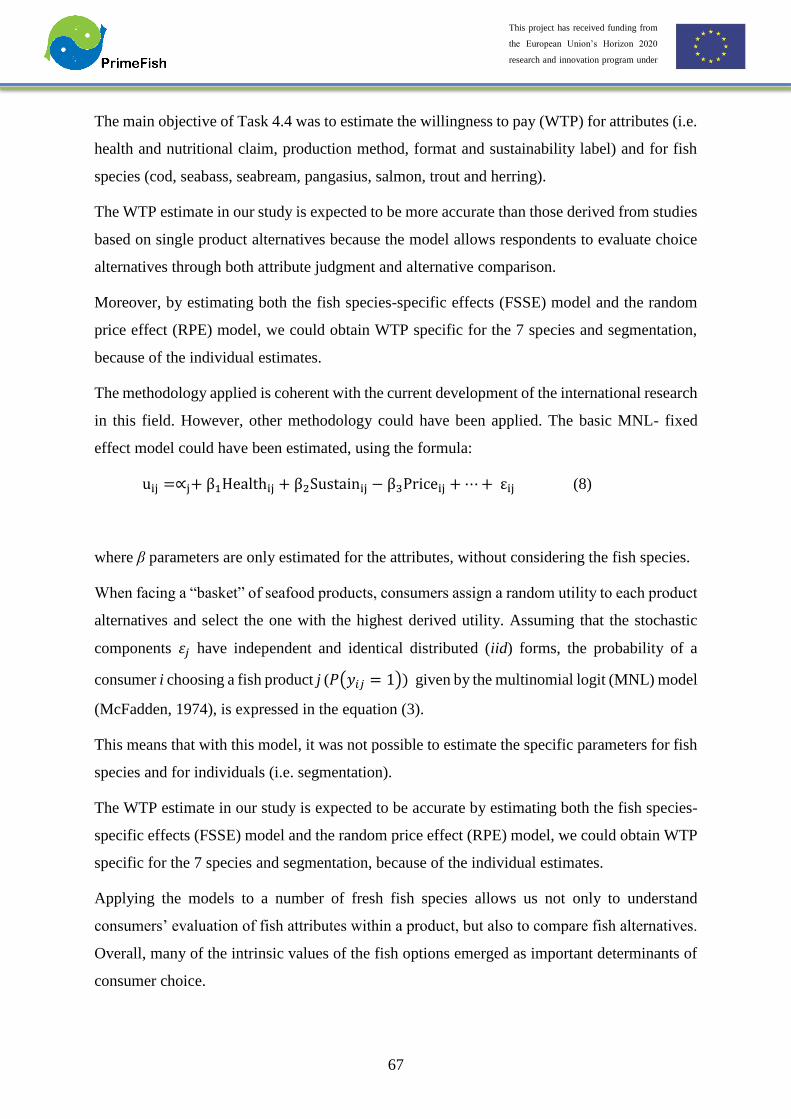
67





The main objective of Task 4.4 was to estimate the willingness to pay (WTP) for attributes (i.e.

health and nutritional claim, production method, format and sustainability label) and for fish

species (cod, seabass, seabream, pangasius, salmon, trout and herring).

The WTP estimate in our study is expected to be more accurate than those derived from studies

based on single product alternatives because the model allows respondents to evaluate choice

alternatives through both attribute judgment and alternative comparison.

Moreover, by estimating both the fish species-specific effects (FSSE) model and the random

price effect (RPE) model, we could obtain WTP specific for the 7 species and segmentation,

because of the individual estimates.


in this field. However, other methodology could have been applied. The basic MNL- fixed

effect model could have been estimated, using the formula:

uij =∝j+ β1Healthij + β2Sustainij − β3Priceij + ⋯ + εij (8)

where β parameters are only estimated for the attributes, without considering the fish species.

When facing a “basket” of seafood products, consumers assign a random utility to each product

alternatives and select the one with the highest derived utility. Assuming that the stochastic

components 휀𝑗 have independent and identical distributed (iid) forms, the probability of a

consumer i choosing a fish product j (𝑃(𝑦𝑖𝑗 = 1)) given by the multinomial logit (MNL) model

(McFadden, 1974), is expressed in the equation (3).

This means that with this model, it was not possible to estimate the specific parameters for fish

species and for individuals (i.e. segmentation).

The WTP estimate in our study is expected to be accurate by estimating both the fish species-

specific effects (FSSE) model and the random price effect (RPE) model, we could obtain WTP

specific for the 7 species and segmentation, because of the individual estimates.

Applying the models to a number of fresh fish species allows us not only to understand

consumers’ evaluation of fish attributes within a product, but also to compare fish alternatives.

Overall, many of the intrinsic values of the fish options emerged as important determinants of

consumer choice.

68





Moreover, using the random price effect (RPE) model we have obtained individuals’ estimates

of the WTP for fish attributes alternatives, therefore allowing more deep analysis, including

market segmentation based the consumers choices.

The main disadvantage of the method is related with the applied hypothetical choice

experiment; in this case, the consumer choice may not be consistent with actual choices in the

real market (i.e. the hypothetical bias, see Lusk et al. 2011). Therefore, the results of WTP may

be overestimated. However, we have applied techniques to reduce the gap between hypothetical

and real choice, i.e. including a cheap-talk script in the choice experiment. Moreover, the actual

response task imposed respondents to select one single (fish) product only from each of the

choice sets provided. With this simplification of the purchasing process we effectively

eliminated the complexity of purchasing multiple goods. One further weakness in our study is

associated with not including all potential quality attributes, in particular country of origin. We

have decided to exclude the attribute origin because this attribute has already been deeply

studied in the literature (Carlucci et al., 2015). Moreover, a huge effect of the domestic origin

has been documented in previous studies: 145% WTP by Stefani et al. (2012), 108% by

Mauracher et al. (2013), 100% by McClenachan et al. (2016). We have evaluated that this effect

might have overwhelmed the impact of other attributes on the consumers’ choices. Therefore,

since other attributes have been studied much less, we have

The methodology applied (fish species-specific effects model and random price effect model)

was directly based on the type of data collected. Based on the objective of the task (WTP

estimated in 5 countries with online survey), the use of an online (hypothetical) choice

experiment was straightforward. Therefore, the models applied, in our opinion, provide the best

possible estimates for the attributes and species analysed.

We recommend that data be collected using proper methodology, in particular by evaluating

carefully the choice of the attributes and levels to be analysed. Including more attributes would

have increased the complexity of the choice task, which might have shifted the choice

behaviours toward the choice of the “Non-option” rather than evaluating the attributes in the

experiment.

Regarding the methodology used to analyse the data, we recommend to estimate mixed logit

models, such as the fish species-specific effects (FSSE) model and the random price effect

(RPE) model that we have estimated. In this way, it will be possible to obtain WTP estimates

specific for the fish species and a market segmentation, because of the individual estimates.

69





15 Fisheries and aquaculture competitiveness index

The Fisheries and Aquaculture Competitiveness Index (FACI) developed in deliverable 5.1 is

modelled on the Fisheries Competitive Index (FCI) developed by the Directorate of Fresh Fish

Prices in Iceland and the Norwegian College of Fishery Science at the University of Tromsø in

2004-2005 (Verðlagsstofa skiptaverðs, 2009). The FACI though expands on the FCI in two

directions. First, by developing a national-level FACI that also includes aquaculture. Second,

by designing a firm-level index that is intended to capture the views of operators of individual

firms and is therefore less complex.

The national-level FACI consists of 144 items, whereof 44 are taken from the WEF Global

Competitiveness Index, 19 are based on data obtained from national, public sources and 81 are

based on answers from a survey conducted among specialists in each country. Whereas the

information taken from the GCI analyses the overall competitiveness of the nation, the other

sources will throw light on the competitiveness of the fisheries and aquaculture sectors. The

firm-level FACI is based on a survey which in the case of firms engaged in the harvesting,

processing or marketing of wild capture fish consists of 40 questions, and in the case of

aquaculture firms consists of 45 questions

The firm-level FACI builds heavily on the theories of Porter (1998), taking into consideration

all five aspects of competition outlined by Porter. This index is mostly intended for operators

of fisheries and aquaculture firms who wish to analyse the competitive standing of their firm.

The index consists of 40 questions – 45 in the case of aquaculture – that together yield a solid

measure of competitiveness. Here the results of a survey that was put to a limited number of

firm operators are presented. Once the PrimeDSS in PrimeFish becomes operational it will be

possible to access a computerised version of the firm-level FACI, complete the survey online

and then obtain a measure of the competitiveness of the firm, both by analysing the data and

comparing the competitive standing of the firm to that of other firms. Each question uses a

seven-level Likert scale.

The national-level FACI is a comprehensive measure that includes both factors influencing

each country’s overall competitiveness, as well as factors that specifically relate to the fisheries

and aquaculture sectors. Most of the indicators related to overall competitiveness are taken from

the Global Competitiveness Index, published by the World Economic Forum (2016), but

information on the other, more specific indicators was obtained through surveys and from

public data collection agencies.

70





The national-level FACI consists of three pillars; (I) basic requirements, (II) efficiency

enhancers, and (III) innovation and sophistication. In contrast to the firm-level FACI, the

national-level FACI yields a weighted overall score for each country, as well as a weighted

score for each pillar and the sub-indexes contain therein. Basic requirements weigh 30% of the

total score, efficiency enhancers 50% and innovation and sophistication 20%.

71





16 Boom-and-bust model

This section discusses the methodology used in deliverable 5.2 “Boom-and-bust” model which

aimed to develop simulation and prediction models that could be used to predict price hehaviour

and give early-warning signals of a potential “boom-and-bust” cycle.

The statistical model used for the prices prediction is based on Robust Monitoring of Time

Series approach. Time series often contain outliers and level shifts or structural changes, and

these unexpected events are of the utmost importance in the forecasting of prices. The presence

of such unusual events can easily mislead conventional time series analysis and yield erroneous

conclusions. The model provides a unified framework for detecting outliers and level shifts in

short time series that may have a seasonal pattern. The methodology was developed to detect

potential fraud cases in time series of imports into the European Union, and we have borrowed

it because it is particularly suited to the type of data and phenomena we have to manage

(Barabesi et al, 2016; Fried et al., 2012; Galeano and Pena, 2013; Riani et al., 2012), Rousseeuw

and van Driessen, 2006; Salini et al., 2015; FSDA).

The formal approach of the model is described in Perrotta et al. (2018), which contains

methodology for robustly analysing a time series which contains a trend, a seasonal component

(possibly time varying) and a level shift in an unknown position, as well as isolated or

consecutive outliers.

The model is particularly suitable for the task at hand because it introduces a new robust

approach to model and monitor nonlinear time series with a possible level shift. A fast algorithm

was developed and applied to several real and artificial datasets. The automatic detection of

level shift avoids the alternative and most common way of splitting in the parts before and after

the break, after which each part can be analysed separately.

The model is especially relevant for this study because it can be applied to data sets which are

not very long (less than 36 months), such as are frequently found in the fisheries sectors. The

models also make it possible to manage any significant price changes over the period observed

and therefore to make better forecasts. It is also quite easy to interpret the results for persons

with non-statistical background. The model also offers the possibility to calculate robust

confidence bands in the forecasts, therefore to define the risk linked to the forecasts. Finally,

the model is innovative, as the method applied represents an improvement on previous models.

72






in this field. However, other methodologies could have been applied, such as ARCH and

GARCH models. ARCH (autoregressive conditionally heteroscedastic) model is a model for

the variance of a time series. ARCH models are used to describe a changing, possibly volatile

variance. Although an ARCH model could possibly be used to describe a gradually increasing

variance over time, most often it is used in situations in which there may be short periods of

increased variation. GARCH (generalized autoregressive conditionally heteroscedastic) model

uses values of the past squared observations and past variances to model the variance at time t.

The main strength of this method is that it works work well with not very long times series (less

than 36 months), as are often found in fisheries, the ability to manage any significant price

changes over the period observed and therefore to make better forecasts, the ease of

interpretation of results for persons with non-statistical background and the possibility to

calculate the confidence bands in the forecasts, therefore to define the risk linked to the forecasts

and its robustness to the presence of isolated or consecutive outliers.

The weaknesses of the model, in relation to the aims of the project, are its inability to not foresee

the boom and bust cycles in future periods compared to the observed data. This incapacity is

not related to the model chosen in particular, but it is common to each statistical model.

The methodology applied was chosen to suit the task at hand and the nature of the data collected.

The model applied provides, in our opinion, the best possible estimate of the cycle in prices

time series for the species analysed.

Future work should be based on data collected using a well defined methodology and set up in

a well organised database. This study was based on the following variables taken from

EUMOFA; period (month, year), monthly prices, country, flow type (import or export), partner

country (imported from or exported to), fish species, market (first sale/landing, wholesale,

retail).

73





17 Latent class analysis and multinomial logistic regression

Latent class analysis (LCA) (Lazarsfeld and Henry, 1968) was used in deliverable 5.4 which

built on the demand and consumer analysis conducted in WP4. The deliverable introduced a

robust model that could be used to analyse the likelihood that new seafood products launched

will be successful by identifying certain consumer segments and matching them with products

on offer.

Latent class analysis has been suggested as a model-based tool for regular market segmentation

(Wedel & Kamakura, 2000) and international segmentation (Steenkamp & ter Hofstede, 2002).

By “model-based,” we mean that there is a statistical model that is assumed to come from the

population from which the data was gathered (Vermunt and Magidson, 2002a; Vermunt and

Magidson, 2002b). LCA is the state-of-the art segmentation method because of rigorous,

objective and probabilistic results. Common areas of application include marketing research

(eg. consumers segmentation), survey research, sociology, psychology and education. The most

common use of LCA is to discover case subtypes (or confirm hypothesized subtypes) based on

multivariate categorical data, a use which is perfectly in line with our objective.

LCA is a statistical method for finding subtypes of related cases, i.e. latent classes (they are

called latent because a case's class membership is not directly observed) from multivariate

categorical data (Marateb et al., 2014), in way analogous to cluster analysis. That is, given a

sample of subjects (consumers) measured on several manifest (observed) variables (e.g. items),

one wishes to know if there is a small number of basic groups into which cases fall (Uebersax,

2006). The latent class model seeks to stratify the cross-classification table of manifest variables

by a latent unordered categorical variable that eliminates all confounding between the manifest

variables (Jaspers et al., 2016).

Beyond LCA, traditional cluster analysis is used for the “segmentation” of sample data.

Additionally, in identifying groups both methods aim at maximization which in the case of LCA

concerns the log-likelihood function while in the case of traditional clustering a given criteria

is maximized.

The advantages of LCA (probabilistic model) over cluster analysis (heuristic model) can be

summarized as follows: less arbitrary choice of the grouping criterion; easier to use with

different scales; flexibility in the choice of probability distributions; restraints can be rigorously

defined and checked; formal criteria to decide number of classes (information criteria) and the

74





possibility to insert covariates for the definition and description of classes (and for validation

purposes); Vermunt and Magidson (2002a) in a comparison between LCA and K-mean

clustering have evidenced that LCA errors of classification are systematically lower than those

of traditional cluster analysis.

Also, LCA is suitable for binary, ordered-category and Likert-scale, or nominal data and there

is no technical barrier to analyzing models that combine categorical and continuous data

(Lazarsfeld and Henry, 1968).

LCA supposes a simple parametric model and uses observed data to estimate parameter values

for the model. The model parameters are (i) the prevalence of each latent classes, and (ii)

conditional response probabilities, i.e. the probabilities, for each combination of latent class,

item or variable (the items or variables are termed the manifest variables), and response level

for the item or variable, that is a randomly selected member of that class will make that response

to that item/variable (Collins and Lanza, 2010).

Essentially, LCA allows to obtain cross-classification tables of equal dimension to the observed

table of manifest variables, and, following the assumption of conditional independence, the

proportion of observations in each latent class, and the probabilities of observing each response

to each manifest variable, conditional on latent class. Observations with similar sets of

responses on the manifest variables will tend to cluster within the same latent classes

(Hagenaars and McMutcheon, 2009). In this way, the LCA output will contains elements which

enables quick comparisons of the observed cell counts to the cell counts predicted by the latent

class model (Uebersax, 2006; Linzer and Lewis, 2011).

LCA defines latent classes by the criterion of conditional independence, that is conditional upon

values of this latent variable, responses to all of the manifest variables are assumed to be

statistically independent. This means that, within each latent class, each variable is statistically

independent of every other variable (Magidson and Vermunt (2002). For example, within a

latent class that corresponds to a distinct consumer segment the presence/absence of one

preference is viewed as unrelated to presence/absence of all others. Paul Lazarsfeld (Lazarsfeld

and Henry, 1968), the main originator of LCA, argued that this criterion leads to the most

natural and useful groups.

An advantage of LCA as compared with other clustering techniques is the variety of tools

available for assessing model fit and for determining the appropriate number of latent classes.

(Linzer and Lewis, 2011).

75





In some applications, the number of latent classes will be selected for primarily theoretical

reasons, in other cases, however, the analysis may be of a more exploratory nature, with the

objective being to locate the best fitting or most parsimonious model. The researcher may then

begin by fitting a complete “independence” model with C = 1, and then iteratively increasing

the number of latent classes by one until a suitable fit has been achieved (Linzer and Lewis,

2011).

Parsimony criteria seek to strike a balance between over- and under-fitting the model to the data

by penalizing the log-likelihood by a function of the number of parameters being estimated

(Linzer and Lewis, 2011). The two most widely used parsimony measures are the Bayesian

information criterion (BIC) (Schwartz, 1978) and Akaike information criterion (AIC) (Akaike,

1973). Preferred models are those that minimize values of the BIC and/or AIC.

The BIC will usually be more appropriate for basic latent class models because of their relative

simplicity (Lin and Dayton 1997). Calculating Pearson’s χ2 goodness of fit and likelihood ratio

chi-square (G2) statistics for the observed versus predicted cell counts is another method to help

determine how well a particular model fits the data (Goodman 1970).The entropy of a model is

also used as a model selection criterion, either by itself or together with other statistics (Larose

et al., 2016).

Problems related to the sample size, the adequate number of classes and the sparseness problem

have been discussed in literature (for more details please see Muthen and Muthen (2002), W.H.

Finch, K.C. Bronk (2011), Wurpts and Geiser (2014).

A LCA model can be expressed as follows. Let 𝑋 represent the latent variable and 𝑌𝑙 one of the

L observed or manifest variables, where 1 ≤ 𝑙 ≤ 𝐿. Moreover, let C be the number of latent

classes and 𝐷𝑙 the number of levels of 𝑌𝑙. A particular LC (latent classes) is enumerated by the

index x, x = 1, 2, ..., C, and a particular value of 𝑌𝑙 by 𝑦𝑙, 𝑦𝑙= 1, 2, ..., 𝐷𝑙. The vector notation Y

and y is used to refer to a complete response pattern.

The basic idea underlying any type of LC model is that the probability of obtaining response

pattern y, 𝑃(Y = y), is a weighted average of the C class-specific probabilities 𝑃(Y = y|𝑋 =

𝑥); that is,

𝑃(𝑌 = 𝑦) = ∑ 𝑃(𝑋 = 𝑥)𝑃(Y = y|𝑋 = 𝑥)

𝐶

𝑥=1

… … … (1)

76





Here, 𝑃(𝑋 = 𝑥) denotes the proportion of persons belonging to LC 𝑥.

In the classical LC model, this basic idea is combined with the assumption of local

independence. The 𝐿 manifest variables are assumed to be mutually independent within each

LC, which can be formulated as follows:

𝑃(𝐘 = 𝐲|𝑋 = 𝑥) = ∏ 𝑃(𝑌𝑙 = 𝑦𝑙𝐿𝑙=1 |𝑋 = 𝑥)..................................(2)

After estimating the conditional response probabilities 𝑃(𝑌𝑙 = 𝑦𝑙|𝑋 = 𝑥), comparing these

probabilities between classes shows how the classes differ from each other, which can be used

to name the classes. Combining the two basic equations (1) and (2) yields the following model

for 𝑃(𝐘 = 𝐲) marginal probabilities:

𝑃(𝐘 = 𝐲) = ∑ 𝑃(𝑋 = 𝑥)𝐶𝑥=1 ∏ 𝑃(𝑌𝑙 = 𝑦𝑙

𝐿𝑙=1 |𝑋 = 𝑥) (3)

The model is formulated for nominal indicators 𝑌𝑙 and consequently a multinominal logit

distribution is hypothesized for the conditional probability to obtain 𝑦𝑙 to l, given the affiliation

to the latent class x, 𝑃(𝑌𝑙 = 𝑦𝑙|𝑋 = 𝑥).

The conditional probability is parameterized as follows

𝑃(𝑌𝑙 = 𝑦𝑙|𝑋 = 𝑥) =𝑒𝑥𝑝(𝜂𝑦𝑙|𝑥)

∑ 𝑒𝑥𝑝(𝜂𝑦𝑙

′|𝑥)

𝐷𝑙

𝑦𝑙′=1

(4)

Where the linear term 𝜂𝑦𝑙|𝑥 = 𝛽𝑦𝑙+ 𝛽𝑦𝑙𝑥, the parameter 𝛽𝑦𝑙

is the intercept and 𝛽𝑦𝑙𝑥 is the

effect of the latent variable X on the indicator 𝑌𝑙.

In the same way, the probability associated with the latent variable X has a nominal logit

distribution:

𝑃(𝑋 = 𝑥) =𝑒𝑥𝑝(𝜂𝑥)

∑ 𝑒𝑥𝑝(𝜂𝑥′)𝐶𝑥′=1

(5)

Similarly to cluster analysis, one of the purposes of LC analysis might be to assign individuals

to latent classes. The probability of belonging to LC x – often referred to as posterior

membership probability – can be obtained by the Bayes rule,

77





𝑃(𝑋 = 𝑥|𝐘 = 𝐲) =𝑃(𝑋 = 𝑥)𝑃(𝐘 = 𝐲|𝑋 = 𝑥)

𝑃(𝐘 = 𝐲) (6)

The most common classification rule is modal assignment, which amounts to assigning each

individual to the LC with the highest 𝑃(𝑋 = 𝑥|𝐘 = 𝐲).

The parameters of LC models are typically estimated by means of maximum likelihood (ML):

ln ℒ = ∑ ln 𝑃(𝑌|𝑦𝑖)𝐼𝑖=1 (7)

Where i is a particular pattern of response, I is the number of all potential patterns of response,

(𝐼 = ∏ 𝐷𝑙𝐿𝑙=1 ) and 𝑃(𝐘 = 𝐲𝑖).

Among the most popular numerical methods for solving the Maximum Likelihood Estimation

(MLE) problem is the Expectation-Maximization (EM) algorithm (Dempster et al., 1977). The

EM algorithm treats the estimation of LC model parameters as an estimation problem similar

to those for missing data (i.e. multiple imputation). More details about the model and the

parameter estimation are provided in Lazarsfeld and Henry (1968), Goodman (1974);

Haberman (1979), Clogg (1995), Agresti (2002) and Bartholomew, Knott and Moustaki (2011).

In most LC analysis applications, one not only wishes to build a classification model based on

a set of responses, but also to relate the class membership to explanatory variables. In a more

explanatory study, one may wish to build a predictive or structural model for class membership

whereas in a more descriptive study the aim would be to simply profile the latent classes by

investigating their association with external variables (Vermunt, 2010). The latent class

regression model (LCRM) generalizes the basic latent class model by permitting the inclusion

of covariates to predict individuals' latent class membership (Dayton and Macready, 1988;

Hagenaars and McCutcheon, 2009).

In the LC analysis literature two ways for dealing with covariates have been proposed: a “one-

step” and a “three-step” approach. The former involves simultaneous estimation of the LC

(measurement) model of interest with a logistic regression (structural) model in which the latent

classes are related to a set of covariates (Vermunt, 2010). Instead, the “three-step" approach

estimates the basic latent class model, calculates the predicted posterior class membership

78





probabilities and then uses these values as the dependent variable(s) in a regression model with

the desired covariates. Since the “one-step” presents certain disadvantages – for example, it

limits the number of covariates that can be considered in the model (please see Vermunt, 2010)

- we use the “three-step" approach in order to avoid such limitation. In a subsequent step, this

allows us to predict the consumer segment and perform a matching between segmentation and

firms’ characteristics, in order to detect the best segment for the firm. Accounting to this, the

causal relationship firm-to-consumer segment will be explained by multinomial logistic

regression models where the consumer segment will be the dependent variable and the selected

covariates (es. organic, wild, cheap ...etc) will be the choice factors. Once the company has

selected the variables (X) –the estimated coefficients of multinomial logistic regression will be

employed:

𝑙𝑜𝑔𝑖𝑡(𝑃) = ln(𝑂𝑑𝑑𝑠𝑖) = (𝑙𝑛𝑃(𝑐𝑙𝑎𝑠𝑠𝑖)

𝑃(𝑐𝑙𝑎𝑠𝑠𝑟 )) = X𝛽𝑖

where 𝑖 = 1, … , 𝑘 − 1, k = number of classes discovered by LCA, r = reference class, X is

the design matrix (with the independent variables) and 𝛽𝑖is the coefficients vector for the

modality logit i

Finally, we compute the membership probabilities �̂�𝑖 = 𝑒𝑋𝛽

1+𝑒𝑋𝛽 (by coefficients) for each i class

in order to obtain the results in terms of best class, i.e. the best membership probability, in other

terms, the “best” segment. From the algorithm we obtain the association between product

characteristics and the segment, according to the best fit (highest membership probability).

The method described above was employed using primary data (cross-sectional) collected

through an online survey in Summer 2017; including 800 consumers (no restrictions on

frequency) of at least one of the target species (salmon, cod, seabream, seabass, herring, trout,

and pangasius) and be fairly or completely involved in the fish buying process in their

households in each country (Germany, Italy, France, Spain, UK) for a total of 4.000

representative responses along age, gender, education, geography. The survey was designed

based on extant literature and in-depth consumer interviews done in WP 4.2.

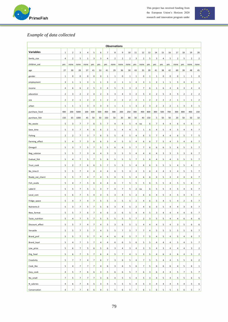
79





Example of data collected

Observations

Variables 1 2 3 4 5 6 7 8 9 10 11 12 13 14 15 16 17 18 19 20

family_size 4 2 5 1 3 3 4 2 2 2 3 2 5 3 4 5 2 5 2 2

children_eat yes none none none yes yes yes none none none yes none yes yes yes yes none yes none none

age 27 30 28 57 41 53 41 29 36 30 43 35 39 41 38 42 69 39 48 45

gender 1 0 0 0 0 0 1 1 0 1 1 0 1 1 0 0 0 1 1 0

employment 3 1 1 3 1 1 3 2 1 1 4 3 1 2 1 1 5 4 3 1

income 4 6 6 2 5 3 4 5 5 3 2 7 6 1 6 4 6 3 4 4

education 2 3 2 2 4 2 3 3 4 3 2 5 4 2 5 4 5 2 2 2

sea 2 2 1 2 2 1 2 2 2 2 2 1 2 2 2 2 1 1 1 2

urban 1 1 1 3 3 3 3 1 1 1 3 2 3 2 2 2 1 3 3 1

purchace_food 400 200 5000 100 600 500 400 300 200 250 300 400 800 300 500 700 300 800 400 150

purchace_fish 150 65 1000 45 50 50 150 50 30 80 50 40 150 5 50 50 20 50 50 10

No_waste 5 3 7 7 6 5 7 4 4 5 4 na 6 7 4 4 6 4 6 7

Save_time 5 3 7 4 6 6 2 5 4 4 5 1 6 4 5 4 5 4 4 7

Fishing 2 2 7 3 7 6 5 5 6 5 4 6 5 7 4 4 6 5 7 5

Farming_effect 5 4 7 3 6 6 3 4 5 5 4 6 6 7 5 4 5 4 6 7

Omega3 5 3 7 5 7 5 5 6 6 5 7 7 6 6 6 5 6 5 5 7

Neg_substan 5 5 7 3 4 4 3 3 5 5 4 4 6 4 3 3 5 3 6 7

Evaluat_fish 5 4 7 5 7 5 6 5 5 5 7 5 6 4 5 4 3 5 5 7

Trust_cook 5 2 7 6 6 5 7 5 5 5 4 6 6 5 5 5 4 5 4 7

No_time.0 5 5 7 4 4 4 4 6 5 3 4 3 6 4 4 3 4 5 5 7

Ready_eat_charct 5 5 7 4 7 4 5 4 5 5 4 6 6 4 5 4 4 4 6 7

Fish_availa 5 4 7 5 6 4 4 6 7 5 5 5 6 5 5 4 5 5 4 7

Label.0 5 5 7 5 1 3 7 4 7 5 2 na 6 5 5 4 5 4 6 7

Local_com 5 6 7 5 4 3 5 3 4 5 2 6 6 4 5 4 5 4 5 7

Fridge_space 5 4 7 4 7 5 5 3 5 5 2 4 6 5 4 5 4 2 6 7

Nutrients.0 5 3 7 5 7 5 6 3 4 5 2 4 6 3 5 4 4 3 6 7

New_format 5 5 7 6 7 4 6 3 6 5 4 4 5 3 4 4 4 4 6 7

Taste_nutrition 5 4 7 5 7 5 5 5 5 5 7 2 3 5 5 4 4 6 6 6

Discount_effect 5 5 7 4 7 4 5 3 6 5 1 4 4 4 5 4 3 5 6 6

Versatile 5 5 7 5 7 4 5 5 7 5 7 7 4 5 5 5 5 5 6 7

Brand_pref 5 5 7 3 7 4 4 6 6 5 7 7 5 4 5 4 5 4 6 7

Brand_loyal 5 4 7 5 7 4 4 6 6 5 6 5 5 4 4 4 5 4 5 7

Low_price 5 6 7 5 6 5 6 3 4 3 4 3 5 4 3 4 4 4 3 2

Org_food 5 6 7 5 7 6 4 5 7 4 1 3 5 4 6 4 6 4 5 2

Creativity 5 7 7 4 7 6 7 3 6 5 4 7 5 5 4 4 5 5 6 2

Cook_like 5 4 7 7 7 4 6 3 6 5 6 7 5 6 6 6 4 5 6 1

Easy_cook 4 5 7 6 6 3 5 6 6 5 7 6 3 6 4 4 5 7 5 7

No_smell 7 5 7 7 7 3 6 4 5 5 4 5 3 4 5 4 5 5 6 5

N_calories 4 6 7 6 5 3 5 5 5 5 4 5 3 4 4 4 5 4 5 6

Conservation 4 7 7 6 6 4 5 5 6 5 7 6 1 6 5 5 5 6 5 7

80





Gen_appear 6 3 7 7 7 5 6 6 7 6 7 7 1 6 5 4 5 6 6 6

Easy_digest 6 6 7 7 5 3 5 5 6 5 4 7 3 4 4 4 5 4 5 7

Quality_price 6 4 7 7 7 4 6 6 7 5 7 7 1 6 5 4 6 7 6 6

Animal_welfare 5 5 7 6 7 4 6 4 5 5 4 5 1 6 5 4 5 5 5 5

No_time 5 5 7 6 7 4 5 4 5 5 4 5 1 6 5 4 3 5 5 7

Natural 6 4 7 6 7 4 6 5 6 5 7 7 1 6 5 4 6 6 6 6

Healthy 6 3 7 6 7 5 6 6 7 5 7 7 1 6 5 4 6 6 6 6

Discount 7 3 7 7 6 5 5 4 6 5 7 4 1 5 4 4 5 6 5 5

Environ_friend 7 4 7 6 7 5 5 4 5 5 4 5 1 5 4 4 5 5 5 3

Nutrients 5 5 7 6 7 5 6 4 5 5 4 6 1 4 4 4 5 5 6 7

Texture 5 6 7 7 7 5 6 4 6 5 7 7 1 6 5 5 6 5 6 7

Origin_guarant 5 7 7 7 6 5 6 4 7 5 4 7 1 5 5 5 5 na 5 7

Sust_certif 5 5 7 7 7 4 6 4 6 5 4 6 1 5 5 4 5 5 6 6

tot_consumption 5 5 5 4 5 5 6 6 5 6 5 4 5 2 5 4 5 5 5 5

Salmon 5 5 3 0 5 4 5 6 4 0 4 3 4 0 5 4 3 3 4 5

Seabream 0 4 0 0 0 0 5 0 2 5 0 2 4 0 0 0 0 0 0 0

Seabass 4 6 0 0 0 0 4 0 2 0 0 0 5 0 0 0 0 0 0 0

Trout 3 4 4 0 0 0 4 0 2 5 0 0 4 0 0 0 0 0 0 0

Cod 0 0 0 3 0 5 4 0 3 5 4 2 5 0 5 0 4 4 4 0

Herring 0 5 0 0 0 0 4 0 4 5 0 0 0 0 0 0 0 0 0 0

Pangasius 0 0 0 0 0 0 0 0 3 0 0 0 0 2 0 0 0 0 0 0

Whole_fish 3 4 0 2 0 0 5 0 3 6 0 0 5 0 0 0 0 0 3 5

Fresh_fillet 3 0 0 0 0 5 5 0 3 5 0 3 4 0 5 2 0 0 0 0

Fillet_frozen 0 0 4 2 4 0 0 6 3 6 3 0 5 2 0 3 4 3 3 0

Ready_eat 5 0 5 0 0 0 0 4 0 6 3 0 0 0 0 0 0 4 0 5

Ready_Cook 4 4 0 3 0 0 0 0 3 6 4 0 5 0 0 4 0 3 3 0

Marinated 0 5 0 0 0 0 0 0 0 5 0 0 0 0 0 4 0 0 0 0

Dry 0 6 0 0 0 0 0 0 3 0 0 0 0 0 0 0 0 0 0 0

Smoked 5 5 0 0 0 0 5 0 3 5 0 0 0 0 4 0 0 2 3 0

Salad 0 0 0 0 0 0 0 0 0 0 0 0 0 0 0 0 3 0 0 0

Spread 6 0 0 0 0 0 5 4 4 6 0 0 0 0 5 0 0 5 0 0

Canned 0 0 0 0 0 0 0 0 0 5 4 0 0 0 0 0 4 0 2 0

Wild_farmed 3 5 1 6 1 4 4 5 3 6 4 1 2 4 2 5 2 2 1 2

Cheap_expensive 1 4 7 1 1 3 4 5 2 4 1 4 4 3 4 4 3 3 4 4

Natural_enchance 1 5 1 1 1 5 3 3 2 4 1 5 2 1 1 4 1 1 1 5

Bones_boneless 6 3 7 7 7 3 4 7 7 7 7 3 4 7 5 4 5 7 6 7

Fresh_frozen 4 3 1 1 7 4 1 5 4 3 7 2 2 4 1 3 6 4 3 5

Local_national 4 4 7 1 3 4 1 6 4 3 4 4 2 4 4 3 5 6 4 4

EU_NEU 4 4 7 1 1 5 3 2 3 1 4 1 4 4 1 2 6 1 4 4

Trustp_n 4 5 7 1 4 5 3 4 3 1 4 4 4 4 4 4 4 3 4 5

Brand_n 4 3 7 1 1 4 5 4 4 5 1 4 4 1 3 3 3 4 4 5

Organic_n 4 4 1 1 6 5 3 6 3 2 7 4 4 7 1 4 3 4 4 7

Prepared_n 4 4 7 7 7 3 6 6 6 5 4 7 4 4 7 4 6 4 6 2

Traditional_n 4 3 1 1 1 4 2 2 3 3 1 1 3 1 1 4 2 1 1 5

81





Family 3 4 7 1 1 6 4 2 5 4 1 2 4 1 3 2 3 2 3 1

Fishsaler 4 3 7 4 6 4 7 1 4 1 1 3 7 3 3 3 2 3 4 3

supermarket 5 4 7 2 4 3 7 3 4 1 1 2 6 1 3 3 1 2 5 6

Mass_adv 7 5 7 2 1 3 2 3 5 1 1 1 2 1 1 3 1 1 4 4

Social_media 5 6 7 2 1 3 1 1 4 1 1 1 2 1 1 1 1 1 3 1

Science 6 5 7 2 1 3 3 1 4 1 1 1 2 1 1 1 2 1 3 2

Doctor 6 4 7 3 1 4 4 1 3 1 1 1 2 1 1 1 2 1 3 3

Industry 5 3 7 2 1 4 5 1 4 1 1 1 6 4 1 1 1 1 2 3

Label 6 2 7 3 1 3 7 1 5 1 1 3 3 4 3 4 5 2 5 5

Friends 4 4 7 3 1 4 3 2 4 3 1 1 4 1 2 2 3 1 3 1

Consum_org 6 3 7 2 1 3 4 1 5 1 1 3 3 1 3 1 4 1 5 1

Salmon*_format__Fresh_fil* 0 0 0 0 0 0 1 0 1 0 0 1 0 0 1 1 0 0 0 0

Salmon_format__Frozen_fil 0 0 1 0 1 0 0 1 1 0 1 0 1 0 0 0 0 0 0 0

Salmon_format__Ready_eat 1 0 1 0 0 0 0 0 0 0 0 0 0 0 0 0 0 0 0 1

Salmon_format__Ready_cook 0 0 0 0 0 0 0 0 0 0 0 0 0 0 0 0 0 1 1 0

Salmon_format__Smoked 1 1 0 0 0 0 1 0 0 0 0 0 0 0 0 0 0 1 1 0

Salmon_format__Canned 0 0 0 0 0 0 0 0 0 0 0 0 0 0 0 0 0 0 0 0

Salmon_format__Marinated 0 0 0 0 0 0 0 0 0 0 0 0 0 0 0 0 0 0 0 0

Salmon_format__Whole 0 0 0 0 0 0 1 0 0 0 0 0 1 0 0 0 0 0 0 0

Salmon_format__Dry 0 0 0 0 0 0 0 0 0 0 0 0 0 0 0 0 0 0 0 0

Salmon_format__Salad 0 0 0 0 0 0 0 0 0 0 0 0 0 0 0 0 1 0 0 0

Salmon_format__Spread_ 1 0 0 0 0 0 1 0 0 0 0 0 0 0 0 0 0 0 0 0

Evolution 5 5 7 4 5 4 2 6 5 4 4 5 5 4 5 4 5 4 3 5

*Data of formats available for all species.

Output of latent class analysis (LCA) and multinomial logistic regression (example for the

Spanish dataset)

LCA was performed to obtain segmentations of markets (consumers side) based on a response to 27-items:

Omega3, Fish evaluation, Trust to cook, No time, Ready to eat, Availability, Label, Local, New format, Taste over

nutrition, Versatile, Value for money, Preferred brand, Brand loyalty, Creativity, Like to cook, Appearance,

Conservation, Easy to cook, Easy to digest, Natural, Healthy, Environmental friendly, Nutrients, Texture,

Traceability, Sustainability.

Example of output

R Output of the LCA

Conditional item response (column) probabilities,

by outcome variable, for each class (row)

$Omega3

1 2 3 4 5 6

class 1: 0.0000 0.0351 0.1567 0.7723 0.0359 0.0000

class 2: 0.0000 0.0000 0.0167 0.1116 0.7253 0.1464

class 3: 0.0683 0.1907 0.1104 0.1909 0.3019 0.1379

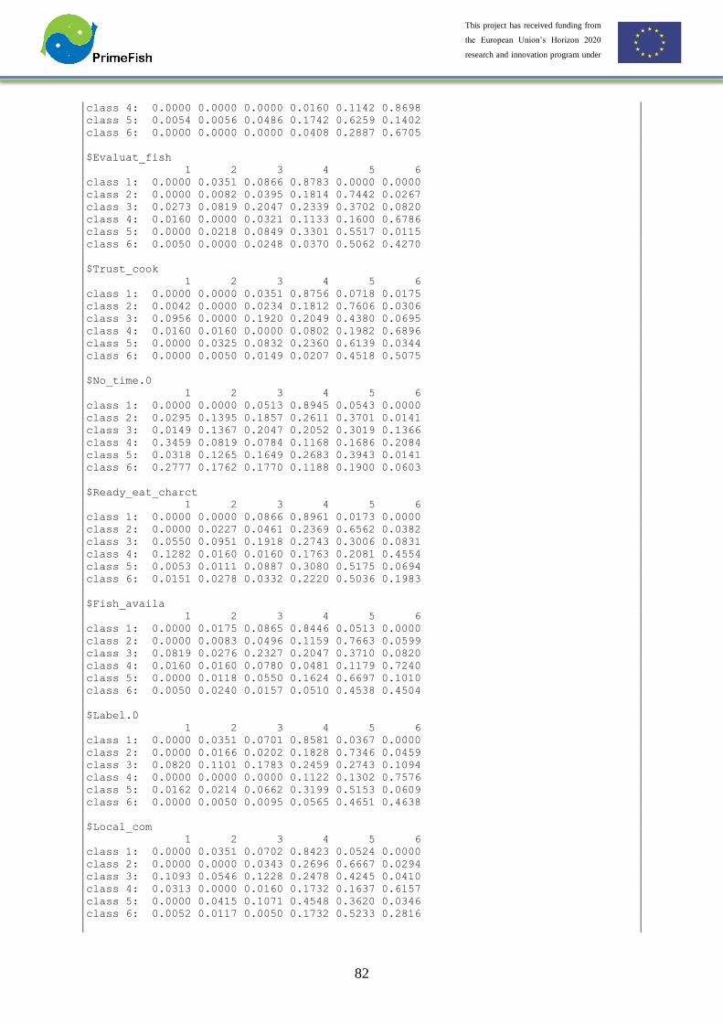
82





class 4: 0.0000 0.0000 0.0000 0.0160 0.1142 0.8698

class 5: 0.0054 0.0056 0.0486 0.1742 0.6259 0.1402

class 6: 0.0000 0.0000 0.0000 0.0408 0.2887 0.6705

$Evaluat_fish

1 2 3 4 5 6

class 1: 0.0000 0.0351 0.0866 0.8783 0.0000 0.0000

class 2: 0.0000 0.0082 0.0395 0.1814 0.7442 0.0267

class 3: 0.0273 0.0819 0.2047 0.2339 0.3702 0.0820

class 4: 0.0160 0.0000 0.0321 0.1133 0.1600 0.6786

class 5: 0.0000 0.0218 0.0849 0.3301 0.5517 0.0115

class 6: 0.0050 0.0000 0.0248 0.0370 0.5062 0.4270

$Trust_cook

1 2 3 4 5 6

class 1: 0.0000 0.0000 0.0351 0.8756 0.0718 0.0175

class 2: 0.0042 0.0000 0.0234 0.1812 0.7606 0.0306

class 3: 0.0956 0.0000 0.1920 0.2049 0.4380 0.0695

class 4: 0.0160 0.0160 0.0000 0.0802 0.1982 0.6896

class 5: 0.0000 0.0325 0.0832 0.2360 0.6139 0.0344

class 6: 0.0000 0.0050 0.0149 0.0207 0.4518 0.5075

$No_time.0

1 2 3 4 5 6

class 1: 0.0000 0.0000 0.0513 0.8945 0.0543 0.0000

class 2: 0.0295 0.1395 0.1857 0.2611 0.3701 0.0141

class 3: 0.0149 0.1367 0.2047 0.2052 0.3019 0.1366

class 4: 0.3459 0.0819 0.0784 0.1168 0.1686 0.2084

class 5: 0.0318 0.1265 0.1649 0.2683 0.3943 0.0141

class 6: 0.2777 0.1762 0.1770 0.1188 0.1900 0.0603

$Ready_eat_charct

1 2 3 4 5 6

class 1: 0.0000 0.0000 0.0866 0.8961 0.0173 0.0000

class 2: 0.0000 0.0227 0.0461 0.2369 0.6562 0.0382

class 3: 0.0550 0.0951 0.1918 0.2743 0.3006 0.0831

class 4: 0.1282 0.0160 0.0160 0.1763 0.2081 0.4554

class 5: 0.0053 0.0111 0.0887 0.3080 0.5175 0.0694

class 6: 0.0151 0.0278 0.0332 0.2220 0.5036 0.1983

$Fish_availa

1 2 3 4 5 6

class 1: 0.0000 0.0175 0.0865 0.8446 0.0513 0.0000

class 2: 0.0000 0.0083 0.0496 0.1159 0.7663 0.0599

class 3: 0.0819 0.0276 0.2327 0.2047 0.3710 0.0820

class 4: 0.0160 0.0160 0.0780 0.0481 0.1179 0.7240

class 5: 0.0000 0.0118 0.0550 0.1624 0.6697 0.1010

class 6: 0.0050 0.0240 0.0157 0.0510 0.4538 0.4504

$Label.0

1 2 3 4 5 6

class 1: 0.0000 0.0351 0.0701 0.8581 0.0367 0.0000

class 2: 0.0000 0.0166 0.0202 0.1828 0.7346 0.0459

class 3: 0.0820 0.1101 0.1783 0.2459 0.2743 0.1094

class 4: 0.0000 0.0000 0.0000 0.1122 0.1302 0.7576

class 5: 0.0162 0.0214 0.0662 0.3199 0.5153 0.0609

class 6: 0.0000 0.0050 0.0095 0.0565 0.4651 0.4638

$Local_com

1 2 3 4 5 6

class 1: 0.0000 0.0351 0.0702 0.8423 0.0524 0.0000

class 2: 0.0000 0.0000 0.0343 0.2696 0.6667 0.0294

class 3: 0.1093 0.0546 0.1228 0.2478 0.4245 0.0410

class 4: 0.0313 0.0000 0.0160 0.1732 0.1637 0.6157

class 5: 0.0000 0.0415 0.1071 0.4548 0.3620 0.0346

class 6: 0.0052 0.0117 0.0050 0.1732 0.5233 0.2816

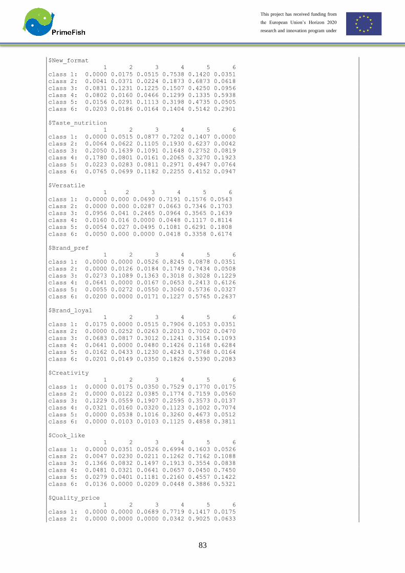
83





$New_format

1 2 3 4 5 6

class 1: 0.0000 0.0175 0.0515 0.7538 0.1420 0.0351

class 2: 0.0041 0.0371 0.0224 0.1873 0.6873 0.0618

class 3: 0.0831 0.1231 0.1225 0.1507 0.4250 0.0956

class 4: 0.0802 0.0160 0.0466 0.1299 0.1335 0.5938

class 5: 0.0156 0.0291 0.1113 0.3198 0.4735 0.0505

class 6: 0.0203 0.0186 0.0164 0.1404 0.5142 0.2901

$Taste_nutrition

1 2 3 4 5 6

class 1: 0.0000 0.0515 0.0877 0.7202 0.1407 0.0000

class 2: 0.0064 0.0622 0.1105 0.1930 0.6237 0.0042

class 3: 0.2050 0.1639 0.1091 0.1648 0.2752 0.0819

class 4: 0.1780 0.0801 0.0161 0.2065 0.3270 0.1923

class 5: 0.0223 0.0283 0.0811 0.2971 0.4947 0.0764

class 6: 0.0765 0.0699 0.1182 0.2255 0.4152 0.0947

$Versatile

1 2 3 4 5 6

class 1: 0.0000 0.000 0.0690 0.7191 0.1576 0.0543

class 2: 0.0000 0.000 0.0287 0.0663 0.7346 0.1703

class 3: 0.0956 0.041 0.2465 0.0964 0.3565 0.1639

class 4: 0.0160 0.016 0.0000 0.0448 0.1117 0.8114

class 5: 0.0054 0.027 0.0495 0.1081 0.6291 0.1808

class 6: 0.0050 0.000 0.0000 0.0418 0.3358 0.6174

$Brand_pref

1 2 3 4 5 6

class 1: 0.0000 0.0000 0.0526 0.8245 0.0878 0.0351

class 2: 0.0000 0.0126 0.0184 0.1749 0.7434 0.0508

class 3: 0.0273 0.1089 0.1363 0.3018 0.3028 0.1229

class 4: 0.0641 0.0000 0.0167 0.0653 0.2413 0.6126

class 5: 0.0055 0.0272 0.0550 0.3060 0.5736 0.0327

class 6: 0.0200 0.0000 0.0171 0.1227 0.5765 0.2637

$Brand_loyal

1 2 3 4 5 6

class 1: 0.0175 0.0000 0.0515 0.7906 0.1053 0.0351

class 2: 0.0000 0.0252 0.0263 0.2013 0.7002 0.0470

class 3: 0.0683 0.0817 0.3012 0.1241 0.3154 0.1093

class 4: 0.0641 0.0000 0.0480 0.1426 0.1168 0.6284

class 5: 0.0162 0.0433 0.1230 0.4243 0.3768 0.0164

class 6: 0.0201 0.0149 0.0350 0.1826 0.5390 0.2083

$Creativity

1 2 3 4 5 6

class 1: 0.0000 0.0175 0.0350 0.7529 0.1770 0.0175

class 2: 0.0000 0.0122 0.0385 0.1774 0.7159 0.0560

class 3: 0.1229 0.0559 0.1907 0.2595 0.3573 0.0137

class 4: 0.0321 0.0160 0.0320 0.1123 0.1002 0.7074

class 5: 0.0000 0.0538 0.1016 0.3260 0.4673 0.0512

class 6: 0.0000 0.0103 0.0103 0.1125 0.4858 0.3811

$Cook_like

1 2 3 4 5 6

class 1: 0.0000 0.0351 0.0526 0.6994 0.1603 0.0526

class 2: 0.0047 0.0230 0.0211 0.1262 0.7162 0.1088

class 3: 0.1366 0.0832 0.1497 0.1913 0.3554 0.0838

class 4: 0.0481 0.0321 0.0641 0.0657 0.0450 0.7450

class 5: 0.0279 0.0401 0.1181 0.2160 0.4557 0.1422

class 6: 0.0136 0.0000 0.0209 0.0448 0.3886 0.5321

$Quality_price

1 2 3 4 5 6

class 1: 0.0000 0.0000 0.0689 0.7719 0.1417 0.0175

class 2: 0.0000 0.0000 0.0000 0.0342 0.9025 0.0633

84





class 3: 0.0957 0.4110 0.1378 0.0956 0.2326 0.0273

class 4: 0.0160 0.0000 0.0000 0.0448 0.1196 0.8196

class 5: 0.0108 0.0054 0.0330 0.1328 0.7513 0.0666

class 6: 0.0050 0.0096 0.0195 0.0327 0.7357 0.1976

$Easy_cook

1 2 3 4 5 6

class 1: 0.0000 0.0000 0.0000 0.8439 0.1561 0.0000

class 2: 0.0000 0.0000 0.0043 0.1609 0.7971 0.0376

class 3: 0.1652 0.2049 0.2734 0.1232 0.2191 0.0143

class 4: 0.0641 0.0320 0.0000 0.0332 0.1728 0.6978

class 5: 0.0090 0.0000 0.0702 0.3962 0.5027 0.0219

class 6: 0.0513 0.0150 0.0451 0.1861 0.5651 0.1373

$Conservation

1 2 3 4 5 6

class 1: 0.0000 0.0000 0.0176 0.9468 0.0356 0.0000

class 2: 0.0000 0.0000 0.0071 0.0734 0.8782 0.0413

class 3: 0.0821 0.2185 0.2212 0.1641 0.2595 0.0546

class 4: 0.0641 0.0000 0.0000 0.0636 0.1338 0.7385

class 5: 0.0000 0.0165 0.0809 0.3623 0.5402 0.0000

class 6: 0.0200 0.0198 0.0208 0.1231 0.6506 0.1657

$Gen_appear

1 2 3 4 5 6

class 1: 0.0000 0.0174 0.0526 0.8253 0.0872 0.0175

class 2: 0.0000 0.0000 0.0042 0.0727 0.7948 0.1283

class 3: 0.2731 0.2329 0.2336 0.0133 0.1924 0.0547

class 4: 0.0321 0.0000 0.0000 0.0643 0.0583 0.8454

class 5: 0.0162 0.0275 0.0428 0.2125 0.6438 0.0572

class 6: 0.0050 0.0144 0.0000 0.0518 0.4675 0.4613

$Easy_digest

1 2 3 4 5 6

class 1: 0.0000 0.0000 0.0174 0.9300 0.0526 0.0000

class 2: 0.0000 0.0000 0.0096 0.1292 0.8402 0.0210

class 3: 0.1647 0.2323 0.2462 0.1650 0.1091 0.0826

class 4: 0.0641 0.0000 0.0000 0.0340 0.1876 0.7143

class 5: 0.0266 0.0321 0.1010 0.4594 0.3735 0.0074

class 6: 0.0452 0.0153 0.0353 0.2158 0.5480 0.1404

$Natural

1 2 3 4 5 6

class 1: 0.0000 0.0175 0.0175 0.9300 0.0349 0.0000

class 2: 0.0000 0.0000 0.0042 0.0148 0.8921 0.0889

class 3: 0.1361 0.1639 0.2869 0.2061 0.1374 0.0696

class 4: 0.0313 0.0000 0.0000 0.0161 0.0164 0.9362

class 5: 0.0056 0.0000 0.0324 0.3221 0.6057 0.0342

class 6: 0.0103 0.0050 0.0000 0.0394 0.4895 0.4559

$Healthy

1 2 3 4 5 6

class 1: 0.0000 0.0000 0.0526 0.8274 0.1200 0.0000

class 2: 0.0000 0.0000 0.0000 0.0079 0.8222 0.1699

class 3: 0.1366 0.1775 0.2731 0.1644 0.1800 0.0684

class 4: 0.0160 0.0000 0.0000 0.0000 0.0308 0.9532

class 5: 0.0000 0.0054 0.0109 0.1901 0.7351 0.0585

class 6: 0.0000 0.0000 0.0050 0.0141 0.3788 0.6021

$Environ_friend

1 2 3 4 5 6

class 1: 0.0000 0.0174 0.0350 0.8949 0.0526 0.0000

class 2: 0.0000 0.0000 0.0000 0.0605 0.8901 0.0494

class 3: 0.0956 0.2607 0.3820 0.1094 0.1112 0.0411

class 4: 0.0481 0.0000 0.0000 0.0954 0.1171 0.7394

class 5: 0.0054 0.0000 0.0381 0.5678 0.3831 0.0056

class 6: 0.0000 0.0046 0.0100 0.0635 0.6660 0.2558

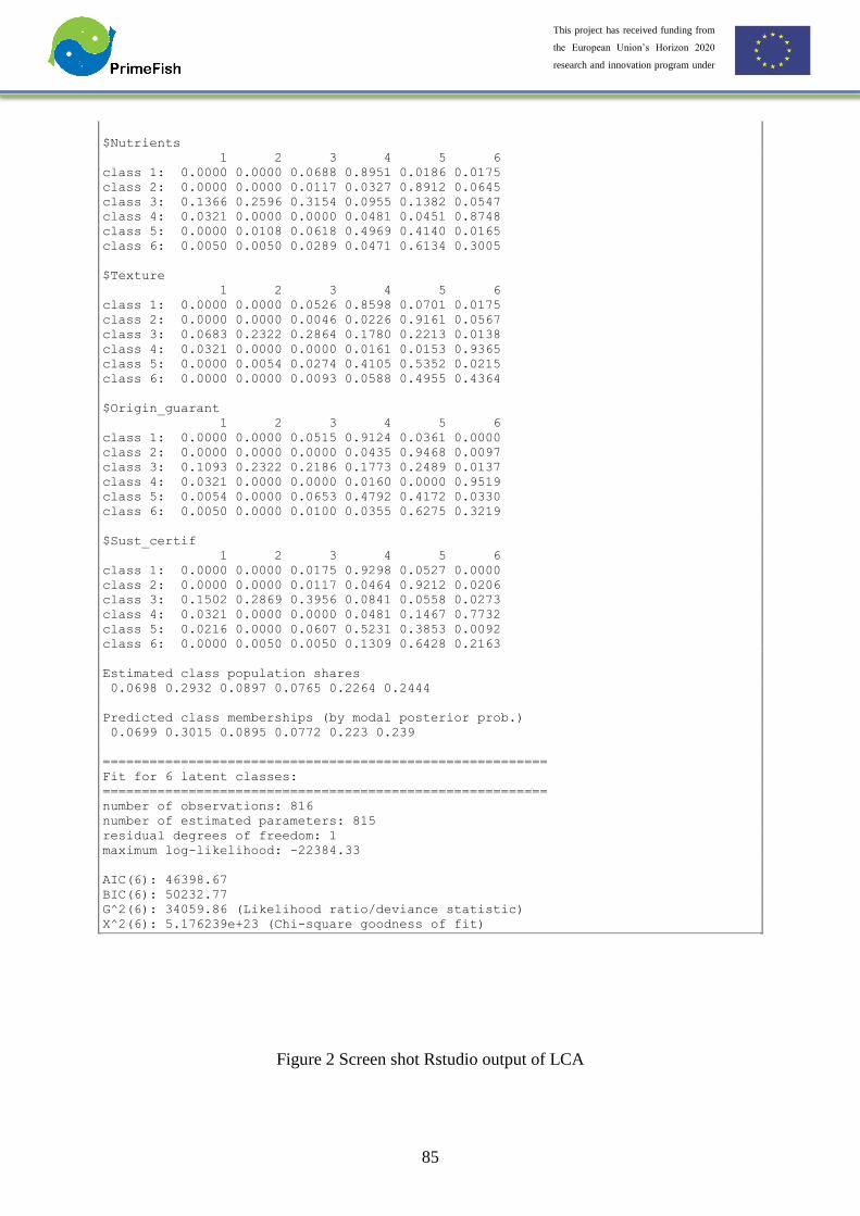
85





$Nutrients

1 2 3 4 5 6

class 1: 0.0000 0.0000 0.0688 0.8951 0.0186 0.0175

class 2: 0.0000 0.0000 0.0117 0.0327 0.8912 0.0645

class 3: 0.1366 0.2596 0.3154 0.0955 0.1382 0.0547

class 4: 0.0321 0.0000 0.0000 0.0481 0.0451 0.8748

class 5: 0.0000 0.0108 0.0618 0.4969 0.4140 0.0165

class 6: 0.0050 0.0050 0.0289 0.0471 0.6134 0.3005

$Texture

1 2 3 4 5 6

class 1: 0.0000 0.0000 0.0526 0.8598 0.0701 0.0175

class 2: 0.0000 0.0000 0.0046 0.0226 0.9161 0.0567

class 3: 0.0683 0.2322 0.2864 0.1780 0.2213 0.0138

class 4: 0.0321 0.0000 0.0000 0.0161 0.0153 0.9365

class 5: 0.0000 0.0054 0.0274 0.4105 0.5352 0.0215

class 6: 0.0000 0.0000 0.0093 0.0588 0.4955 0.4364

$Origin_guarant

1 2 3 4 5 6

class 1: 0.0000 0.0000 0.0515 0.9124 0.0361 0.0000

class 2: 0.0000 0.0000 0.0000 0.0435 0.9468 0.0097

class 3: 0.1093 0.2322 0.2186 0.1773 0.2489 0.0137

class 4: 0.0321 0.0000 0.0000 0.0160 0.0000 0.9519

class 5: 0.0054 0.0000 0.0653 0.4792 0.4172 0.0330

class 6: 0.0050 0.0000 0.0100 0.0355 0.6275 0.3219

$Sust_certif

1 2 3 4 5 6

class 1: 0.0000 0.0000 0.0175 0.9298 0.0527 0.0000

class 2: 0.0000 0.0000 0.0117 0.0464 0.9212 0.0206

class 3: 0.1502 0.2869 0.3956 0.0841 0.0558 0.0273

class 4: 0.0321 0.0000 0.0000 0.0481 0.1467 0.7732

class 5: 0.0216 0.0000 0.0607 0.5231 0.3853 0.0092

class 6: 0.0000 0.0050 0.0050 0.1309 0.6428 0.2163

Estimated class population shares

0.0698 0.2932 0.0897 0.0765 0.2264 0.2444

Predicted class memberships (by modal posterior prob.)

0.0699 0.3015 0.0895 0.0772 0.223 0.239

=========================================================

Fit for 6 latent classes:

=========================================================

number of observations: 816

number of estimated parameters: 815

residual degrees of freedom: 1

maximum log-likelihood: -22384.33

AIC(6): 46398.67

BIC(6): 50232.77

G^2(6): 34059.86 (Likelihood ratio/deviance statistic)

X^2(6): 5.176239e+23 (Chi-square goodness of fit)

Figure 2 Screen shot Rstudio output of LCA

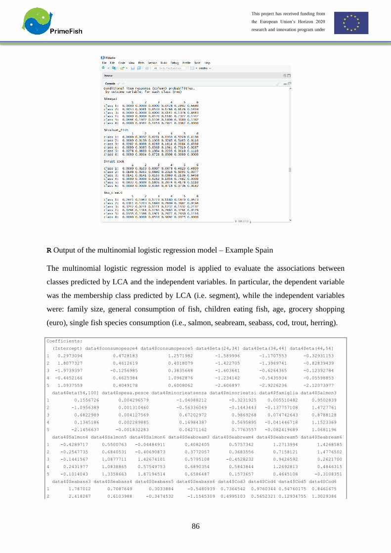
86





R Output of the multinomial logistic regression model – Example Spain

The multinomial logistic regression model is applied to evaluate the associations between

classes predicted by LCA and the independent variables. In particular, the dependent variable

was the membership class predicted by LCA (i.e. segment), while the independent variables

were: family size, general consumption of fish, children eating fish, age, grocery shopping

(euro), single fish species consumption (i.e., salmon, seabream, seabass, cod, trout, herring).

Coefficients:

(Intercept) data4$consumopesce4 data4$consumopesce5 data4$eta(24,34] data4$eta(34,44] data4$eta(44,54]

1 0.2973094 0.4728183 1.2571982 -1.589996 -1.1707553 -0.32931153

2 1.8077327 0.4612619 0.4018079 -1.422705 -1.3969741 -0.82839439

3 -1.9739397 -0.1256985 0.3835648 -1.603641 -0.6264365 -0.12392784

4 -0.4452166 0.6625384 1.0962876 -1.234142 -0.5435934 -0.05598853

5 1.0937559 0.4049178 0.6008062 -2.606897 -2.9226236 -2.12073977

data4$eta(54,100] data4$spesa.pesce data4$minorieatsenza data4$minorieatsi data4$famiglia data4$Salmon3

1 0.1556726 0.004296579 -1.04088212 -0.3231925 0.005510482 0.9502839

2 -1.0956389 0.001310460 -0.56336049 -0.1443443 -0.137757108 1.4727761

3 0.6822989 0.004127569 0.67202972 0.9869268 0.074742643 0.8788128

4 0.1345186 0.002289885 0.16984387 0.5695895 -0.041446718 1.1523369

5 -2.1456637 -0.001832283 0.04271162 0.7763557 -0.082419689 1.0681196

data4$Salmon4 data4$Salmon5 data4$Salmon6 data4$Seabream3 data4$Seabream4 data4$Seabream5 data4$Seabream6

1 -0.4289717 0.5500763 -0.04484911 0.4082405 0.5757342 1.2713994 1.4268585

2 -0.2547735 0.6840531 -0.40690873 0.3772057 0.3683556 0.7158121 1.4776502

3 -0.1441567 1.0877711 1.42674101 0.5795108 -0.4528232 0.9426592 0.2621700

4 0.2431977 1.0838865 0.57549753 0.6890354 0.5843844 1.2692813 0.4846315

5 -0.1014043 1.3358663 1.87194514 0.6586487 0.1573657 0.4645108 -0.3108351

data4$Seabass3 data4$Seabass4 data4$Seabass5 data4$Seabass6 data4$Cod3 data4$Cod4 data4$Cod5 data4$Cod6

1 1.787012 0.7087649 0.3033884 -0.5480939 0.7364542 0.9760344 0.54760175 0.8461675

2 2.418267 0.6103988 -0.3474532 -1.1545309 0.4995103 0.5652321 0.12934755 1.3029386

87





3 2.411934 0.8804017 0.7302333 1.3500697 0.3377865 0.3893280 0.08413534 1.5699073

4 1.957777 0.2970830 -0.1270199 -0.2003194 0.3439874 0.4209879 0.06306292 1.8822597

5 1.488974 0.7338300 0.3692678 -0.7582140 0.6031583 0.6934653 0.34053803 2.6161425

data4$Trout3 data4$Trout4 data4$Trout5 data4$Trout6 data4$Herring3 data4$Herring4 data4$Herring5

1 0.01202464 -0.09239792 0.85278824 -2.054156 -1.0312133 -2.084904 0.5652518

2 -0.19964316 -0.47704943 0.99951152 -2.026728 -1.2120969 -1.625099 0.8275317

3 -0.45669736 -0.15273321 0.96149430 -2.612997 -0.5372914 -1.243819 0.3560451

4 0.20751409 -0.11084493 1.22037052 -1.264981 -0.8735731 -1.805297 0.5150820

5 -0.45531609 -0.85771683 -0.02781817 -3.021906 -0.4557721 -1.743245 -5.1826654

data4$Herring6

1 0.9446358

2 0.8391341

3 -0.7988211

4 -0.1930439

5 0.8549189

Std. Errors:

(Intercept) data4$consumopesce4 data4$consumopesce5 data4$eta(24,34] data4$eta(34,44] data4$eta(44,54]

1 1.563577 0.9220149 0.9980381 0.8080546 0.8085048 0.8003502

2 1.476542 0.8213385 0.9169525 0.7685004 0.7748194 0.7695325

3 2.020334 1.0734197 1.1520917 1.0085871 0.9777106 0.9752825

4 1.544234 0.8681334 0.9471116 0.7906524 0.7895953 0.7874976

5 1.752954 1.0551986 1.1481569 0.7996336 0.8304464 0.8110439

data4$eta(54,100] data4$spesa.pesce data4$minorieatsenza data4$minorieatsi data4$famiglia data4$Salmon3

1 0.8048454 0.002592744 0.8081178 0.7842342 0.1691948 0.6401885

2 0.7825691 0.002685425 0.7883514 0.7707690 0.1673159 0.6188044

3 0.9633827 0.002813677 1.2636749 1.2413534 0.1967610 0.7523307

4 0.7910497 0.002583327 0.8481132 0.8296457 0.1647242 0.6292378

5 0.8320884 0.003290853 0.9985112 0.9734988 0.1924516 0.7188386

data4$Salmon4 data4$Salmon5 data4$Salmon6 data4$Seabream3 data4$Seabream4 data4$Seabream5 data4$Seabream6

1 0.4301278 0.4987573 1.092470 0.6573433 0.4993213 0.5965440 1.017803

2 0.4261833 0.4932579 1.180985 0.6246743 0.4975014 0.6153992 1.068930

3 0.5330382 0.5803843 1.149629 0.7490687 0.6488793 0.6587961 1.156046

4 0.4145194 0.4858261 1.053722 0.6195433 0.4855465 0.5850670 1.025139

5 0.5325939 0.5708277 1.129700 0.7057845 0.5944129 0.6923235 1.217777

data4$Seabass3 data4$Seabass4 data4$Seabass5 data4$Seabass6 data4$Cod3 data4$Cod4 data4$Cod5 data4$Cod6

1 1.122067 0.5339007 0.5304495 0.8697107 0.5314846 0.4746611 0.4637324 1.601206

2 1.099766 0.5327554 0.5593293 1.0206884 0.5069874 0.4672678 0.4643699 1.596846

3 1.173418 0.6490224 0.6050791 0.9122385 0.6271392 0.5569814 0.5376430 1.663850

4 1.097874 0.5239414 0.5260616 0.8209190 0.5080651 0.4570772 0.4483819 1.528825

5 1.188386 0.6262913 0.6239415 1.3378320 0.6111125 0.5555555 0.5383311 1.620966

data4$Trout3 data4$Trout4 data4$Trout5 data4$Trout6 data4$Herring3 data4$Herring4 data4$Herring5

1 0.5980600 0.5045016 0.8296872 1.198188 0.9448573 0.6425214 1.10707366

2 0.5808465 0.5204504 0.8286506 1.310069 0.9467173 0.6394257 1.11816311

3 0.7392116 0.5979520 0.8864250 1.472868 1.0522261 0.7447944 1.20890106

4 0.5668671 0.4908278 0.8100199 1.122775 0.8970846 0.6123385 1.09779869

5 0.7412302 0.6542961 1.0097868 1.512587 1.0451688 0.9222532 0.04567071

data4$Herring6

1 1.344623

2 1.397914

3 1.733318

4 1.370451

5 1.543647

Residual Deviance: 2389.768

AIC: 2739.768

88





Figure 3 Screen shot of multinomial logistic regression model

R Output of the matching “firm-to-segment “ (Example Spain)

Multinomial logistic regression coefficients were employed for the match of segment (demand)

and product/firm (supply side).

The best class is 2 (membership probability = 0.42)

89





References

Aepli M., 2014. Consumer demand for alcoholic beverages in Switzerland: a two-stage quadratic

almost ideal demand system for low, moderate, and heavy drinking households.

Agricultural and Food Economics, 2(1): 1-27.

Agresti, A. (2002). Categorical Data Analysis. Second Edition. New York: Wiley.

Akaike, H. (1973), "Information theory and an extension of the maximum likelihood principle",

in Petrov, B.N.; Csáki, F., 2nd International Symposium on Information Theory, Tsahkadsor,

Armenia, USSR, September 2-8, 1971, Budapest: Akadémiai Kiadó, pp. 267–281.

Arnason, R. (2003) On productivity and productivity growth in the Icelandic fisheries, in

Competitiveness within the Global Fisheries (Proceedings of a conference held in

Akureyri, Iceland, April 6–7, 2000) (Eds) E. Gudmundsson and H. Valtysson, University

of Akureyri, Iceland, pp. 59–81.

Asche, F., Dahl, R.E., Gordon, D.V., Trollvik, T., and. Aandahl, P. (2011). Demand Growth for

Atlantic Salmon: The EU and French Markets. Marine Resource Economics, 26, 255-265.

Banks J, Blundell R, Lewbel A. Quadratic Engel curves and consumer demand. Rev Econ Stat

1997;79(4):527-539.

Barabesi, L., A. Cerasa, D. Perrotta, and A. Cerioli (2016). Modelling international trade data

with the Tweedie distribution for anti-fraud and policy support. European Journal of

Operational Research 258, 1031–1043.

Bartholomew, D., Knott, M., Moustaki, I., (2011). Latent Variable Models and Factor Analysis:

A Unified Approach, 3rd Edition. Wiley Series in Probability and Statistics

Barnett W.A. and Serlettis A., 2008. Consumer preferences and demand systems, Journal of

Econometrics, Volume 147, Issue 2, December 2008, 210–224.

Bhattacharya, C.B. (1997). Is Your Brand' s Loyalty too Much, too Little, or Just Right?

Explaining Deviations in Loyalty from the Dirichlet Norm. International Journal of Research

in Marketing, 14, 421-435.

Bjørndal, T. (1987) Production economics and optimal stock size in a North Atlantic fishery,

Scandinavian Journal of Economics, 89, 145–64.

Bolwig, S., Ponte, S., du Toit Riisgaard, Lone, A., & Halberg, N. (2010). Integrating poverty and

90





environmental concerns in to value chain analysis. A conceptual framework. Development

Policy Review 28 (2), 28(2), 173–194.

Bush, S. R., Oosterveer, P., Bailey, M., & Mol, A. P. J. (2015). Sustainability governance of chains

and networks: A review and future outlook. Journal of Cleaner Production, 107, 8–19.

http://doi.org/10.1016/j.jclepro.2014.10.019.

Calinski, T. & Harabasz, J. (1974). A Dendrite Method for Cluster Analysis. Communications in

Statistics, 3, 1–27.

Carlucci D., Nocella G., De Devitiis B., Viscecchia R., Bimbo F., Nardone G. (2015). Consumer

purchasing behaviour towards fish and seafood products. Patterns and insights from a sample

of international studies. Appetite 84, 212–227.

Carpentier, A., Guyomard, H., 2001. Unconditional elasticities in two-stage demand systems: An

approximate solution. Am. J. Agric. Econ. 83(1), 222–229.

Charnes, A., W.W. Cooper, and E. Rhodes. 1978. Measuring the Efficiency of Decision Making

Units. European Journal of Operational Research (2):429–44.

Chib, S. and Winkelmann, R. (2001). Markov Chain Monte Carlo Analysis of Correlated Count

Data. Journal of Business and Economic Statistics, 19, 428-435.

Clogg, C.C. (1979) "Some latent structure models for the analysis of Likert-type data." Social

Science Research8:287-301.

Clogg, C.C. (1995).Latent class models. In: Arminger G, Clogg CC, Sobel ME (Eds.), Handbook

of statistical modeling for social and behavioral sciences (Ch. 6; pp. 311-359). New York:

Plenum,.

Coelho, A.B., Aguiar, D. R. Dias de, Eales J. S., 2010. Food demand in Brazil: an application

of Shonkwiler & Yen Two-Step estimation method. Estudos Econômicos (São Paulo)

40(1):186-211.

Coelli, T. J., Rao, D. S. P., O’Donnell, C. J., & Battese, G. E. (2005). An Introduction to

Efficiency and Productivity Analysis (2nd ed.). New York: Springer-Verlag.

Collins L. M. and Lanza S. T., (2010), Latent class and latent transition analysis: with

applications in the social, behavioral, and health sciences, Hoboken, NJ: John Wiley and

Sons, Inc.

91





Cox T.L., Wohlgenant, M.K., 1986. Prices and quality effects in cross-sectional demand analysis.

Am J Agric Econ 68(4):908-919.

Crawford I, Pendakur K. How many types are there? The Economic Journal 2013;123(567):77-

95.

Creel, M.D., and Loomis, J.B. (1990). Theoretical and Empirical Advantages of Truncated Count

Data Estimators for Analysis of Deer Hunting in California. American Journal of Agricultural

Economics 72, 434–441.

Dayton, C.M., Macready, G.B., (1988). Concomitant variable latent class models. Journal of the

American Statistical Association, 83:173–178.

Deaton A., 1998. Quality, quantity, and spatial variation of price. Am Econ Rev: 418-430.

Deaton A., Muellbauer J. Economics and Consumer Behavior. : Cambridge University Press;

1980.

Deb, P., and Trivedi, P.K. (2002). The Structure of Demand for Health Care: Latent Class versus

Two-Part Models. Journal of Health Economics, 21, 601-625.

Dempster, A.P., Laird, N.M., Rubin, D.B., (1977). Maximum Likelihood from Incomplete Data

via the EM Algorithm. Journal of the Royal Statistical Society B, 39, 1–38.

Denison, E. F. (1972). Classification of sources of growth. Review of Income and Wealth, 18(1),

1–25.

Duda, R.O. & Hart, P.E. (1973). Pattern Classification and Scene Analysis, New York: John

Wiley & Sons, Inc.

Edgerton, D.L., Assarsson, B., Hummelmose, A., Laurila, I., Rickertsen, K.,Halvor Vale, P.,

1996. The Econometrics of Demand Systems. Kluwer Academic Publishers, Norwell,

MA.

Eggert, H. and Tveterås, (2013) Productivity development in Icelandic, Norwegian and Swedish

fisheries, Applied Economics, 45:6, 709-720.

Farrell, M. (1957). The Measurement of Productive Efficiency. Journal of the Royal Statistical

Society. Series A (General), 120(3), 253-290. doi:10.2307/2343100.

92





Fiebig, D.G., Keane, M.P., Louviere, J.J, & Wasi, N. (2010). The generalized multinomial logit

model: accounting for scale and coefficient heterogeneity. Marketing Science, 29(3), 393-421.

Finch, W.H., Bronk, K.C., (2011). Conducting Confirmatory Latent Class Analysis Using Mplus

.Struct Equ Modeling.18, 132–151.

Fried, R., K. Schettlinger, and M. Borowski (2012). Package ‘robfilter’. CRAN. URL:

http://www.statistik.tu-dortmund.de/fried.html.

FSDA Toolbox: http://rosa.unipr.it/fsda.html.

Galeano, P. and D. Peña (2013). Finding outliers and unexpected events in linear and nonlinear

possible multivariate time series data. In C. Becker, R. Fried, and S. Kuhnt (Eds.),

Robustness and Complex Data Structures. Festschrift in Honour of Ursula Gather,

pp. 255–273. Springer.

Gerdesmeier D., Roffia B., Lenarcic A. An alternative method for identifying booms and busts

in the euro area housing market, European Central Bank Working papers (Paper: 1493,

17.11.2012), 2012

Gereffi, G., & Fernandez-Stark, K. (2011). Global Value Chain Analysis: A Primer. Center on

Globalization, Governance & Competitivenes (CGGC), 1–39.

Globalvaluechains.org, 2011. Duke University. Global Value Chains Initiative.

Gobillon, L., and, Wolff, F.C. (2015). Evaluating the Law of One Price Using Micro Panel Data:

The Case of The French Fish Market. American Journal of Agricultural Economics, 98, 134-

153.

Goodman, L.A., (1970). The multivariate analysis of qualitative data: Interactions among

multiple classifications. J. Amer. Stat. Assoc. 65:226-256.

Greene, W.H., & Hensher, D.A. (2003). A latent class model for discrete choice analysis: contrasts

with mixed logit. Transportation Research B, 37(8), 681-698.

Gustavsen, G.W., Rickertsen, K., 2014. Consumer cohorts and purchases of nonalcoholic

beverages. Empirical Economics 46(2): 427-449.

Haberman, S.J. (1979). Analysis of Qualitative Data, Vol 2, New Developments. New York:

Academic Press.

Hagenaars, J. A., & McCutcheon, A. L. (2009). Applied latent class analysis. Cambridge:

https://www.bis.org/cbhub/list/author/author_2039/index.htm

https://www.bis.org/cbhub/list/author/author_9538/index.htm

93





Cambridge University Press.

Hanley, N., Barbier, E., 2009. Pricing Nature: Cost-benefit Analysis and Environmental

Policy. Edward Elgar.

Hannesson, R. (1983) Bioeconomic Production Function in Fisheries: Theoretical and Empirical

Analysis Canadian Journal of Fisheries and Aquatic Sciences, 1983, 40 (7), 968-982.

Hannesson, R. (2007a) Growth accounting in a fishery, Journal of Environmental Economics and

Management, 53, 364–76.

Hannesson, R. (2007b) A note on the stock effect, Marine Resource Economics, 22, 69–75.

Harvey A.C., “Time Series Models”, Second Ed., MIT Press, 1993

Harvey, A. C. and T. Proietti. Readings in Unobserved Components Models. Advanced Texts in

Econometrics. Oxford University Press, 2005.

Heien D., Wesseils, C.R., 1990. Demand systems estimation with microdata: a censored

regression approach. Journal of Business & Economic Statistics8(3):365-371.

Hellerstein, D.M. (1991). Using Count Data Models in Travel Cost Analysis with Aggregate Data.

American Journal of Agricultural Economics, 73, 860–866.

Hensher, D.A., Rose, J.M., Greene, W.H., 2007. Applied Choice Analysis. A Primer.

Cambridge University Press.

Houthakker H.S., 1952. Compensated Changes in Quantities and Qualities Consumed, The

Review of Economic Studies, Vol. 19, No. 3 (1952 - 1953): 155-16.

Irz X. Modelling physical quantities of food and nutrients consumed from aggregate data - with

an application to Finland. Agricultural Economics 2010;41(3-4):293-304.

Jorgenson, D. W., & Griliches, Z. (1967). The Explanation of Productivity Change. The Review

of Economic Studies, 34(3), 249-283.

Kalman, R. E., “A New Approach to Linear Filtering and Prediction Problems”, Trans. ASME,

Journal of Basic Engineering, pp. 35-45, March 1960.

Kaplinsky, R., & Morris, M. (2001). A Handbook for Value Chain Research. Institute for

Development Studies: Brighton, UK, (September), 1–109.

94





Kau, A.K., and Ehrenberg, A.S.C. (1984. Patterns of Store Choice. Journal of Marketing Research,

21, 399-409.

Kendrick, J. W. (1961). Productivity the United Trends in States. Princeton: National Bureau of

Economic Research.

Kumbhakar, S. C. & Lovell, C. A. K. 2000. Stochastic frontier analysis, Cambridge University

Press, New York, USA.

Lancaster, K.J. (1966). A New Approach to Consumer Theory. Journal of Political Economics

74(2):132-57.

Larose C, Harel O, Kordas K, Dey DK. Latent Class Analysis of Incomplete Data via an Entropy-

Based Criterion. Statistical methodology. 2016;32:107-121.

doi:10.1016/j.stamet.2016.04.004.

Lazarsfeld, P. F. & Henry, N. W., (1968). Latent structure analysis. Boston: Houghton Mifflin.

Retrieved August 16, 2013 (http://www.getcited.org/pub/101262987).

Lewbel A. The Rank of Demand Systems: Theory and Nonparametric Estimation. Econometrica

1991;59(3):711-730.

Lewbel A, Pendakur K. Tricks with Hicks: The EASI Demand System. Am Econ Rev

2009;99(3):827-863.

Lin,T. H., Dayton, C.M., (1997). Model Selection Information Criteria for Non-Nested Latent

Class Models. Journal of Educational and Behavioral Statistics, 22(3), 249 – 264.

Linzer, D. and Lewis, J., (2011). poLCA: An R Package for Polytomous Variable Latent Class

AnalysisJournal of Statistical Software, 42,10, 1-29. https://www.jstatsoft.org/v042/i10

Lusk J.L, Roosen J., Shogren J. (2011). The Oxford Handbook of the Economics of Food

Consumption and Policy. Oxford University Press.

Maddala G., 1983. Methods of estimation for models of markets with bounded price variation.

International Economic Review: 361-378.

Marateb, H.R., Mansourian, M., Adibi, P., Farina, D., (2014). Manipulating measurement scales

in medical statistical analysis and data mining: A review of methodologies. Journal of Research

in Medical Sciences : The Official Journal of Isfahan University of Medical Sciences. 19(1):47-

56.

95





Mauracher C., Tempesta T., Vecchiato D. (2013). Consumer preferences regarding the

introduction of new organic products. The case of the Mediterranean sea bass (Dicentrarchus

labrax) in Italy. Appetite 63, 84–91.

McClenachan L., Dissanayake S.T.M., Chen X. (2016). Fair trade fish: consumer support for

broader seafood sustainability. Fish and Fisheries 17, 825–838.

McFadden, D., 1974. Conditional logit analysis of qualitative choice behavior. In:

McGahan, A. M. (2000). How Industries Evolve. Business Strategy Review, 11(3), 1–16.

https://doi.org/10.1111/1467-8616.00143

Meghir, C., and Robin, J.M. (1992). Frequency of Purchase and the Estimation of Demand

Systems. Journal of Econometrics, 53, 53–85.

Munkin, M.K., and Trivedi, P.K. (1999). Simulated Maximum Likelihood Estimation of

Multivariate Mixed-Poisson Regression Models, with Application. Econometrics Journal, 2,

29-48.

Murphy J, Allen PG, Stevens T, Weatherhead D. A Meta-analysis of Hypothetical Bias in Stated

Preference Valuation. Environmental and Resource Economics 2005 03/01;30(3):313-325.

Muthén, L.K., Muthén, B.O., (2002). How to use a Monte Carlo study to decide on sample size

and determine power. Structural equation modeling, 9, 599-620.

Nielsen, M., Smit, J. and Guillen, J. 2009. Market Integration of Fish in Europe. Journal of

Agricultural Economics, Vol. 60, No. 2, 367–385.

Olsen, S.O., K. Toften, D.C. Dopico, A. Tudoran, & A. Kole. (2008). Consumer Evaluation of

Tailor-Made Seafood Products. Improving seafood products for the consumer. Børresen,

T. Eds, CRC Press.

Onozaka, Y., Hansen, H., and, Sørvig, A. (2014). Consumer Product Perceptions and Salmon

Consumption Frequency: The Role of Heterogeneity Based on Food Lifestyle Segments.

Marine Resource Economics, 29, 351-374.

Park JL, Capps O., 1997. Demand for prepared meals by US households. Am J Agric Econ

79(3):814-824.

Pendakur K. Chapter 7: EASI made easier. In: Slottje DJ, editor. Quantifying consumer

preferences Bingley, UK: Emerald; 2009. p. 179.

96





Perrotta, D., Riani. M., Rousseeuw, P. and Hubert, M. (2018). “Robust Monitoring of Time Series

with Application to Fraud Detection”. Manuscript submitted.

Porter, M. E. (1980). Competitive Strategy: Techniques for Analyzing Industries and Competitors.

Competitive Strategy (Vol. 1). https://doi.org/10.1108/eb025476

Porter, M. E. (1998). The Competitive Advantage of Nations. In M. E. Porter (Ed.), On

Competition (pp. 155–196). Harvard Business Review.

Riani, M., Perrotta, D. and Torti, F. (2012). FSDA: A MATLAB toolbox for robust analysis and

interactive data exploration, CHEMOMETRICS AND INTELLIGENT LABORATORY

SYSTEMS, 116, p. 17-32, doi:10.1016/j.chemolab.2012.03.017.

Robin, J.M. (1993). Analysis of the Short-Run Fluctuations of Households’ Purchases. The

Review of Economic Studies, 60, 923-934.

Rousseeuw, P. and K. Van Driessen (2006). Computing LTS regression for large data sets. Data

Mining and Knowledge Discovery 12, 29–45.

Rumelt, R. P. (1991). How much does industry matter? Strategic Management Journal.

https://doi.org/10.1002/smj.4250120302

Salini, S., A. Cerioli, F. Laurini, and M. Riani (2015). Reliable robust regression diagnostics.

International Statistical Review 84, 99–127.

Sandberg, P. (2006) Variable unit costs in output-regulated fisheries, Applied Economics, 38,

1007–18.

Sarle, W.S. (1983). Cubic Clustering Criterion, SAS Technical Report A-108, Cary, NC: SAS

Institute Inc.

Schwarz, G. E., (1978). "Estimating the dimension of a model", Annals of Statistics, 6 (2): 461–

464, doi:10.1214/aos/1176344136, MR 0468014.

Shonkwiler, J.S., and Englin, J. (2005). Welfare Losses Due to Livestock Grazing on Public

Lands: A Count Data Systemwide Treatment. American Journal of Agricultural Economics, 87,

302-313.

Shonkwiler J.S., Yen, S.T., 1999. Two-step estimation of a censored system of equations. Am J

Agric Econ 81(4): 972-982.

97





Solow, R. M. (1957). Technical change and the aggregate production function, The Review of

Economics and Statistics, Vol. 39, No. 3 (Aug., 1957), pp. 312-320.

Steenkamp, J.-B.E.M., & ter Hofstede, F., (2002). International market segmentation: Issues and

perspectives. International Journal of Research in Marketing, 19(3), 185 – 213.

Stefani G., Scarpa R., Cavicchi A. (2012). Exploring consumer’s preferences for farmed sea

bream. Aquaculture International 20(4), 673–691.

Train, K.E., 2009. Discrete Choice Methods with Simulation, second ed. Cambridge

University Press

Uebersax,J., (2006). Latent Class Analysis,. A web-site with bibliography, software, links and

FAQ for latent class analysis; http://www.john-uebersax.com/stat/faq.htm

Uncles, M., Ehrenberg, A.S.C., and Hammond, K. (1995). Patterns of Buyer Behavior:

Regularities, Models, and Extensions. Marketing Science, 14, 71-78.

Uncles, M., and Lee, D. (2006). Brand Purchasing by Older Consumers: An Investigation Using

the Juster Scale and the Dirichlet Model. Marketing Letters, 17, 17-29.

Verðlagsstofa skiptaverðs. (2009). The fisheries competitiveness index 2004-2005. Iceland and

Norway. Available at: https://www.stjornarradid.is/media/atvinnuvegaraduneyti-

media/media/Skyrslur/FCI-report.pdf.

Vermunt, J.K. and Magidson, J., (2002a). “Latent Class Cluster Analysis”, chapter 3 in J.A.

Hagenaars and A.L. McCutcheon (eds.), Advances in Latent Class Analysis. Cambridge

University Press.

Vermunt, J.K. and Magidson J., (2002b), “Latent Class Models for Classification”, Computational

Statistics and Data Analysis, Elsevior

Vermunt, J. K. (2010). Latent Class Modeling with Covariates: Two Improved Three-Step

Approaches. Political Analysis, 18(4), 450-469. Retrieved from

http://www.jstor.org/stable/25792024.

Wächter, P. (2011). Thinking in systems – a primer. Environmental Politics, 20(4), 595–596.

https://doi.org/10.1080/09644016.2011.589585.

Wang, P. (2003). A Bivariate Zero-Inflated Negative Binomial Regression Model for Count Data

with Excess Zeros. Economics Letters, 78, 373-378.

https://www.stjornarradid.is/media/atvinnuvegaraduneyti-media/media/Skyrslur/FCI-report.pdf

https://www.stjornarradid.is/media/atvinnuvegaraduneyti-media/media/Skyrslur/FCI-report.pdf

https://doi.org/10.1080/09644016.2011.589585

98





Wedel, M., and Kamakura, W. A., (2000). Market segmentation: Conceptual and methodological

foundations (2nd ed.). Dordrecht7 Kluwer.

World Economic Forum. 2016. The Global Competitiveness Report 2016-2017. Available at

https://www.weforum.org/reports/the-global-competitiveness-report-2016-2017-1.

Wurpts, I.C., Geiser, C.,(2014). Is adding more indicators to a latent class analysis beneficial or

detrimental? Results of a Monte-Carlo study. Front Psychol.21;5:920. doi:

10.3389/fpsyg.2014.00920. eCollection 2014.

Xie, J., and Myrland, Ø. (2011). Consistent Aggregation in Fish Demand: A Study of French

Salmon Demand. Marine Resource Economics, 26, 267-280.

Zarembka, P. (Ed.), Frontiers of Econometrics. Academic Press, New York, pp. 105–142.

Zeithaml, V.A. (1988). Consumer Perceptions of Price, Quality, and Value: A Means-End Model

and Synthesis of Evidence. Journal of Marketing 52(3): 2-22.

https://www.weforum.org/reports/the-global-competitiveness-report-2016-2017-1

Documents

Project acronym: Project title: Grant agreement No · Authors Sveinn Agnarsson UIce 21/2/2018 SA ... D1.4, brings together all the methods used in PrimeFish and thus gives an overview