Embed Size (px)
DESCRIPTION
Prohaska - Investigation of the Discharge Coefficient for Circular Orifices in Riser Pipes
Citation preview
INVESTIGATION OF THE DISCHARGE COEFFICIENT FOR
CIRCULAR ORIFICES IN RISER PIPES
A Thesis
Presented to
the Graduate School of
Clemson University
In Partial Fulfillment
of the Requirements for the Degree
Master of Science
Civil Engineering
by
Paul David Prohaska II
August 2008
Accepted by:
Dr. Abdul A. Khan, Committee Chair
Dr. Nigel B. Kaye
Dr. Firat Y. Testik
ii
ABSTRACT
The purpose of this study is to examine the discharge coefficient as it pertains to
flow through a circular orifice cut into a thin-walled vertical riser pipe. Perforated riser
pipes are a popular outlet control structure for stormwater detention basins. These
basins are used to store and release stormwater runoff from impervious areas of
developed sites. Federal, state, and local regulatory agencies provide requirements for
the quality of stormwater runoff, as well as the maximum peak discharges from a
developed site. Accurately determining the flow rate from a perforated vertical riser
pipe is crucial to meeting these requirements and protecting the environment from
pollutants found in stormwater runoff.
This study therefore investigated several factors that may affect the value of the
discharge coefficient. A physical model was built and various size riser pipes were
installed in the tank to simulate a detention basin. The discharge through the orifice
was determined by measuring the rate of change of the water level in the tank versus
time. A water level versus volume drained calibration was used to find the rate of
change of volume over time, and hence the discharge coefficient.
The study determined that the discharge coefficient increased with decreasing
head values. The study also found that the discharge coefficient decreased as the height
above the floor was increased, up to a certain point. Another factor found to affect the
discharge coefficient was the orifice diameter to riser diameter, or d D ratio. The

iii
discharge coefficient decreases as the d D ratio is increased. It is postulated that most
of the changes to the discharge coefficient are a result of changes to the contraction of
the jet exiting the orifice.
For orifices away from the influence of the bed, the discharge coefficient vlaues
were normalized and compiled to fit a single curve that could be used to determine the
discharge coefficient for any orifice size in any riser pipe diameter, for a particular head
to orifice diameter ratio.
Multiple orifices in the same vertical plane were investigated as a secondary part
of the study, but no effect on the discharge was found for the orifice spacings tested.
iv
ACKNOWLEDGMENTS
I would like to thank Dr. Abdul Khan for his assistance and guidance throughout
this investigation. Dr. Nigel Kaye’s involvement in this study was invaluable. Without
the help of their knowledge and expertise in every facet of the study, from formulating
the premise to analyzing the results, this investigation could not have been completed. I
would also like to thank the committee member, Dr. Firat Testik, for his comments and
suggestions.

v
TABLE OF CONTENTS
Page
TITLE PAGE ........................................................................................................................ i
ABSTRACT......................................................................................................................... ii
ACKNOWLEDGMENTS..................................................................................................... iv
LIST OF TABLES................................................................................................................ vi
LIST OF FIGURES............................................................................................................. vii
LIST OF SYMBOLS ............................................................................................................ xi
CHAPTER
1. INTRODUCTION....................................................................................................1
2. LITERATURE REVIEW............................................................................................5
3. EXPERIMENTAL SETUP AND METHODOLOGY....................................................19
4. ANALYTICAL PROCEDURE...................................................................................29
5. TEST RESULTS.....................................................................................................34
6. CONCLUSIONS AND RECOMMENDATIONS........................................................67
REFERENCES ...................................................................................................................70
vi
LIST OF TABLES
Table Page
3.1 Description of orifice sizes and d D ratios
investigated in the study..........................................................................27
5.1 Power function parameters from
Figures 5.21 and 5.22...............................................................................51
vii
LIST OF FIGURES
Figure Page
2.1 Large orifice integration setup........................................................................17
3.1 Model Plan View (drawing not to scale) .........................................................20
3.2 Model Section ‘A-A’ (drawing not to scale) ....................................................21
3.3 Perforated Riser Detail (drawing not to scale)................................................23
3.4 Stilling Well Detail (drawing not to scale) .......................................................24
3.5 Tank volume calibration curve of water
level versus volume drained .........................................................................25
4.1 Calibration curve for converting pressure
readings to water level .................................................................................30
4.2 Sample volume drained versus time graph ....................................................31
4.3 Example plot of dC versus h�
........................................................................32
4.4 Comparison of dC with small and large
orifice equation.............................................................................................33
5.1 1.3 cm orifice in a 15.2 cm riser ......................................................................37
5.2 2.5 cm orifice in a 15.2 cm riser ......................................................................37
5.3 3.8 cm orifice in a 15.2 cm riser ......................................................................38
5.4 5.1 cm orifice in a 15.2 cm riser ......................................................................38
5.5 7.6 cm orifice in a 15.2 cm riser ......................................................................39
5.6 1.3 cm orifice in a 30.5 cm riser ......................................................................39
5.7 2.5 cm orifice in a 30.5 cm riser ......................................................................40
viii
List of Figures (Continued)
Figure Page
5.8 5.1 cm orifice in a 30.5 cm riser ......................................................................40
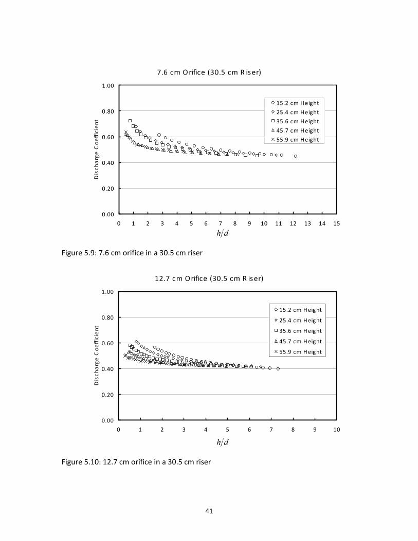
5.9 7.6 cm orifice in a 30.5 cm riser ......................................................................41
5.10 12.7 cm orifice in a 30.5 cm riser....................................................................41
5.11 15.2 cm orifice height for 15.2 cm riser..........................................................43
5.12 25.4 cm orifice height for 15.2 cm riser..........................................................43
5.13 35.6 cm orifice height for 15.2 cm riser..........................................................44
5.14 45.7 cm orifice height for 15.2 cm riser..........................................................44
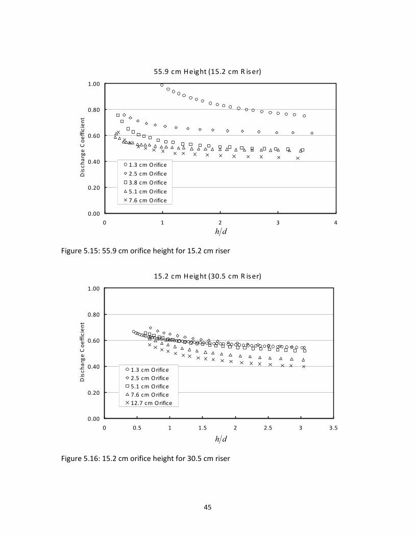
5.15 55.9 cm orifice height for 15.2 cm riser..........................................................45
5.16 15.2 cm orifice height for 30.5 cm riser..........................................................45
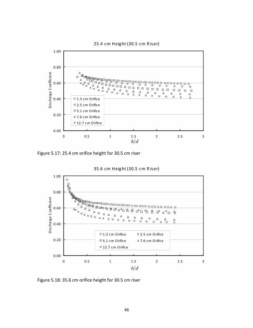
5.17 25.4 cm orifice height for 30.5 cm riser..........................................................46
5.18 35.6 cm orifice height for 30.5 cm riser..........................................................46
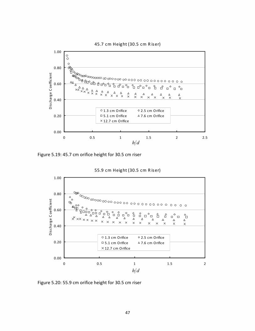
5.19 45.7 cm orifice height for 30.5 cm riser..........................................................47
5.20 55.9 cm orifice height for 30.5 cm riser..........................................................47
5.21 15.2 cm riser upper orifice data and
trend lines .....................................................................................................50
5.22 30.5 cm riser upper orifice data and
trend lines .....................................................................................................50
5.23 Power function parameter, a ,
versus d D ratio..........................................................................................51
5.24 15.2 cm riser compiled data for 20h d = .......................................................... 52
ix
List of Figures (Continued)
Figure Page
5.25 30.5 cm riser compiled data for 20h d = .......................................................... 52
5.26 Determining oC for a particular d D
ratio with 15.2 cm riser .......................................................................................... 53
5.27 Determining oC for a particular d D
ratio with 30.5 cm Riser................................................................................53
5.28 oC for any orifice size and any riser
pipe diameter ( 0.5d D ≤ ) ..........................................................................54
5.29 Determining d oC C for any d D
ratio with any riser pipe size........................................................................55
5.30 Relative error analysis with 0.0417d D = ....................................................56
5.31 Relative error analysis with 0.0833d D = ....................................................56
5.32 Relative error analysis with 0.1667d D = ....................................................57
5.33 Relative error analysis with 0.25d D = ........................................................57
5.34 Relative error analysis with 0.333d D = ......................................................58
5.35 Relative error analysis with 0.4167d D = ....................................................58
5.36 Relative error analysis with 0.5d D = ..........................................................59
5.37 5.1 cm orifice at 2d spacing............................................................................62
5.38 5.1 cm orifice at 4d spacing............................................................................62
5.39 5.1 cm orifice at 6d spacing............................................................................63
5.40 5.1 cm orifice at 8d spacing ............................................................................63
x
List of Figures (Continued)
Figure Page
5.41 7.6 cm orifice at 2d spacing............................................................................64
5.42 7.6 cm orifice at 4d spacing............................................................................64
5.43 7.6 cm orifice at 6d spacing............................................................................65
xi
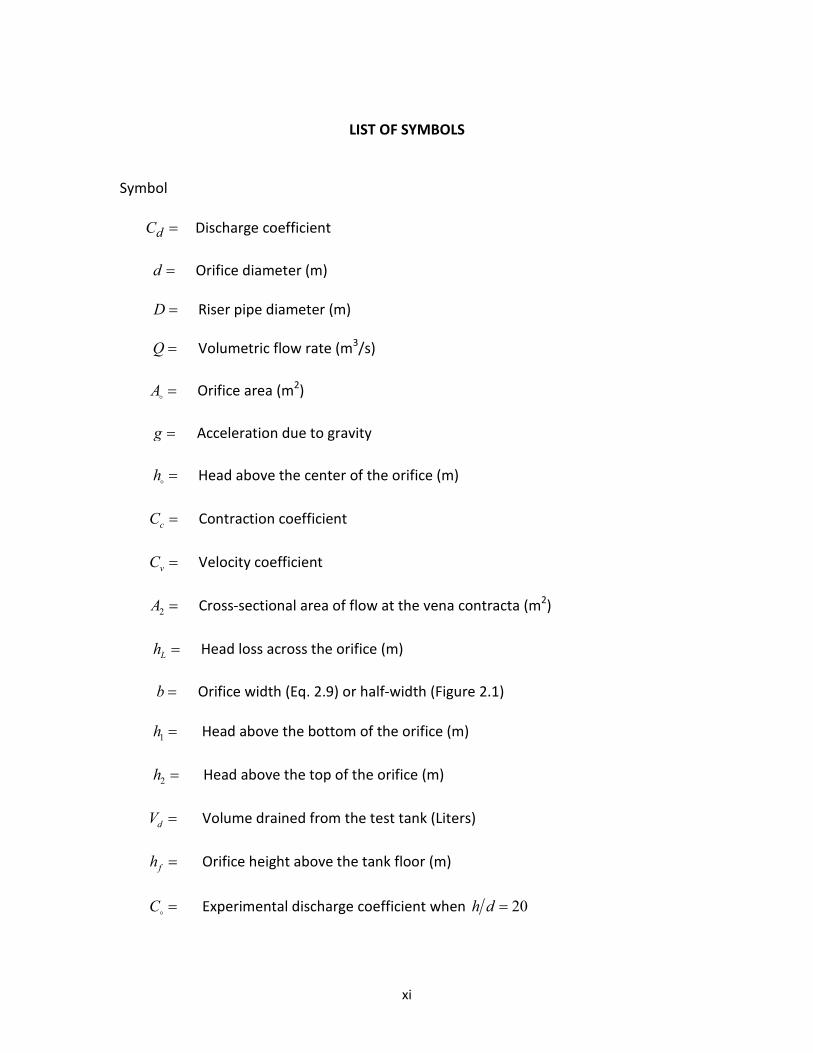
LIST OF SYMBOLS
Symbol
dC = Discharge coefficient
d = Orifice diameter (m)
D = Riser pipe diameter (m)
Q = Volumetric flow rate (m3/s)
A =�
Orifice area (m2)
g = Acceleration due to gravity
h =�
Head above the center of the orifice (m)
cC = Contraction coefficient
vC = Velocity coefficient
2A = Cross-sectional area of flow at the vena contracta (m2)
Lh = Head loss across the orifice (m)
b = Orifice width (Eq. 2.9) or half-width (Figure 2.1)
1h = Head above the bottom of the orifice (m)
2h = Head above the top of the orifice (m)
dV = Volume drained from the test tank (Liters)
fh = Orifice height above the tank floor (m)
C =�
Experimental discharge coefficient when 20h d =
1
CHAPTER 1
INTRODUCTION
As urban and suburban development continues to dominate the cultures of the
world, stormwater runoff rates also continue to increase. Developing land almost
always increases the impervious area when compared to its undeveloped state. Parking
lots, roads, sidewalks, and building roofs are all impervious areas that retain very little
water that falls as precipitation. Instead, most of the rainwater runs off the impervious
areas and onto an adjacent land or into a nearby water body. If not contained,
stormwater runoff can result in flooding and erosion, as well as destroy surrounding
property (Akan and Houghtalen, 2003). Runoff may also contain various pollutants
which can be harmful to people, plants, and animals. Sediment is another harmful
constituent of stormwater runoff. Sediment can carry many harmful substances,
decrease storage capacity of retention ponds, and compromise downstream drainage
systems. Stormwater runoff must be properly managed in order to protect the
environment from land use changes.
In order to contain and manage runoff, the United States Environmental
Protection Agency (US EPA) regulates the discharge of stormwater runoff into natural
water bodies. Developers must obtain permits in order to disturb natural land and
before beginning any construction. These permits, along with various local and state
regulations, require that runoff discharge rates of a developed site not exceed the pre-
2
development peak flow rate. Regulators also require that developers remove potential
pollutants and contaminants to the maximum extent practical (Struble et al., 1997).
Managing stormwater quantity and quality is often done with the use of detention
basins that collect, store, and discharge runoff at appropriate times and rates. The
outlet control structure for these basins is therefore crucial to ensuring the proper
function of these ponds.
One popular outlet control device is a perforated riser, either a constructed box
structure or a vertical pipe cut with orifices of varying size and number. The flow
through these orifices is calculated using a form of the standard orifice equation. For a
box structure, the orifices are cut into a flat wall and represent the typical orifice plate
configuration (orifice in a flat wall). A vertical riser pipe, however, has a curved surface
which may affect the nature of the flow through the orifice. This would be represented
by a change in the discharge coefficient ( )dC . This discharge coefficient has been
studied extensively, but almost exclusively for the case of the orifice in a flat wall.
Studies of orifice flow in a circular pipe are typically limited to cases of pressurized flow
through a sparger or manifold. Here the flow exits a pipe, which is opposite to the case
of a riser pipe outlet structure where the fluid enters the pipe.
The effect of the pipe curvature on the orifice is quantified by relating the orifice
diameter to the riser diameter (d D ratio). This study will investigate a wide range of
d D ratios, ranging from 0.0417 to 0.5. Other factors believed to have an effect on the
discharge coefficient will be investigated here, including the height of an orifice from the
3
basin floor. The proximity of boundaries to an orifice can affect the contraction that the
orifice jet experiences. This may reduce the contraction and increase the discharge
coefficient. Five different orifice heights from the bottom of the tank will be studied to
determine if there is any variation in the discharge coefficient. This may have an
application for detention ponds, as sediment filling the pond will constantly change the
relative orifice height above the floor. The study will also investigate the effect of falling
head on the orifice discharge coefficient. The study utilizes a transient method, in which
water will be allowed to drain naturally as the height is monitored. This will reveal if the
discharge coefficient changes as head values decrease. For lower heads the pressure
distribution across the face of the orifice cannot be neglected, as it is with the standard
orifice equation. This may result in an increase in the discharge coefficient, as the
orifice changes from a small orifice to a large orifice.
To properly investigate the scenario of a perforated vertical riser pipe as an
outlet device for a detention basin, a physical model was built and equipped with
necessary instruments. The model provided for the rapid changing of riser pipes of
various orifice sizes, as well as varying the riser pipe diameter. Data was collected using
LabView and analyzed in Microsoft Excel. The objectives of this study are summarized
below:
• Determine the effects of varying the d D ratio on the orifice discharge
coefficient for orifices cut into a thin-walled pipe,
• Determine the effect of head values on the orifice discharge coefficient,
4
• Determine the effects of varying the orifice height above the basin floor on the
orifice discharge coefficient,
• Investigate two different riser pipe diameters to determine if there is a change in
the discharge coefficient for similar orifice sizes and d D ratios,
• Investigate the effect of multiple orifices and the spacing of orifices on the
discharge coefficient,
Chapter 2 of this study presents a thorough review of current and classical
research concerning orifice discharge coefficients and stormwater runoff quality and
management. Chapter 3 discusses the setup of the physical model and the
experimental procedure employed. Chapter 4 discusses the analytical procedure used
to analyze the test results. Chapter 5 presents the results of the study, along with
appropriate discussions of the data, and Chapter 6 includes conclusions reached and
recommendations for future studies.
5
CHAPTER 2
LITERATURE REVIEW
Introduction
Previous research on orifice discharge coefficients primarily focuses on the
typical case of an orifice cut into a flat wall. Some research discusses orifices cut into a
thin-walled pipe, but this often applies to flow through a sparger or manifold, where the
flow exits a pressurized pipe through multiple orifices cut into the wall of the pipe
(Gregg et al., 2003 and Werth et al., 2005). The case of the stormwater detention pond
with a vertical perforated riser outlet structure is different from this case as there is no
velocity parallel to the orifice. Also, the flow is exiting the orifice through a concave
section in the case of a sparger or manifold, whereas the flow enters the orifice through
a convex section for a vertical riser pipe. Stormwater storage facilities are typically
designed to allow a sufficient residence time of runoff to facilitate the settlement of
sediment and solid particles. Detention basins are also designed to store and release a
specific volume of water at a flow rate which should not exceed that of the pre-
developed condition. Overdesign of outlet structures can lead to rapid dewatering and
deficient water quality of the released water volume (Jarrett, 1993).
6
Background
Increasing urban and suburban development is continuously leading to increases
in stormwater runoff volume and flow rates and can lead to increased flooding and
sometimes severe downstream erosion (Akan and Houghtalen, 2003). Management of
stormwater runoff has become a primary concern for local, state, and federal regulatory
agencies. Two aspects of stormwater management typically dominate regulatory
practices and include water quantity and water quality. Detention basins are widely
used to control both of these aspects. Detention basins capture and store runoff for a
designated period of time, and release the runoff through one or more outlet
structures. A perforated vertical riser is one popular outlet structure used to control
dewatering, defined as the slow, controlled removal of runoff from a detention basin
(Jarrett, 1993). Detention basins manage stormwater volume by the size of the basin
and the stage-storage-outflow relationship. For basins with a regular shape, the
geometry can be used to determine the stage-storage relationship. Contour maps of
the basin are used for unusual-shaped basins (Akan and Houghtalen, 2003). The size
and design of the outlet structure and the maximum stage determine the maximum
flow rate from the detention basin. Most regulatory agencies require that this flow rate
not exceed the pre-development peak flow rate from the disturbed area for a given
storm event.
Water quality is most often addressed by providing sufficient residence time of
runoff in the basin for sediment and other suspended solids to settle out of the runoff.
7
The United States Environmental Protection Agency (US EPA) introduced the National
Pollutant Discharge Elimination System (NPDES), which is a permitting program
designed to help control non-point source pollutants from being discharged into natural
receiving water bodies (Tsihrintzis and Hamid, 1997). The program was launched as part
of the Clean Water Act. Most states have the control to issue permits on behalf of the
US EPA, and states also have the authority to develop their own regulatory practices.
Some states, such as Pennsylvania, enforce a minimum and maximum dewatering time
for a specific rainfall event. This is to ensure adequate time for the runoff to settle out
suspended solids and sediment. A maximum dewatering time ensures that a basin has
enough capacity to store runoff from future storm events (Jarrett, 1993).
Even with local and state regulatory requirements, the efficiency of detention
basins can vary greatly. A study by Millen et al. (1997) investigated different outlet
structures and different basin configurations and evaluated their effectiveness at
removing a particular sediment loading. The study employed a perforated riser outlet
structure as well as a floating riser, or skimmer. Also evaluated was a basin with and
without filter fabric barriers designed to increase the length of the flow path from the
inflow to the outlet structures. The fabric divided the basin into three nearly equal
sections, with openings in the fabric at opposite ends to achieve maximum
effectiveness. A known sediment loading was mixed with the inflow, and the sediment
concentrations at the outflow were measured over time. The basin was designed to
dewater within 24 hours for a 2-year storm event.
8
The research found that the floating skimmer outlet structure retained
significantly more sediment than the perforated riser, and the skimmer also produced a
lower peak flow rate from the basin. In the case of the perforated riser, the fabric
barriers helped to lower the sediment outflow rate. However, the barriers had little
effect on the efficiency of the floating skimmer. The study was conclusive in showing
how certain detention basin design procedures could lead to significantly increased
sediment trapping efficiency. Unfortunately, floating skimmers are rarely used and thus
do not have much use in practical applications (Millen et al., 1997).
The design of detention basins and their associated outlet structures can play a
large role in preventing pollution and erosion of the natural water bodies in which they
discharge. The accurate calculation of flow rate from a perforated riser therefore
becomes critical. Thus, it is necessary to accurately determine the discharge coefficient
for various sizes of orifices cut into a thin-walled pipe.
Discharge coefficient
The standard equation used to estimate flow through a small orifice (small infers
that the pressure distribution across the orifice can be neglected, i.e., head is high
compared to the diameter of the orifice) discharging in atmosphere can be written as:
2dQ C A gh=� �
2.1
Where:
Q = flow rate (m3/s)
9
dC = dimensionless discharge coefficient
A =�
orifice area (m2)
g = acceleration due to gravity
h =�
head above the center of the orifice (m)
An understanding of how the discharge coefficient was developed is crucial to being
able to evaluate its effectiveness. Brater et al. (1996) provides a discussion on the
origins and the development of the discharge coefficient. They describe how the overall
discharge coefficient is actually a combination of two separate coefficients, cC and vC .
cC is a contraction coefficient evaluated at the vena contracta of a jet issuing from an
orifice. Streamlines flowing towards an orifice come from all directions, and in three
dimensions. For all streamlines except those exactly normal to the orifice, there is a
lateral component of velocity which must be dissipated as the water exits the orifice.
These lateral velocity components cause the jet to contract as they round the sharp
edges of an orifice. The flow contracts up to a point, known as the vena contracta. For
a circular orifice, the vena contracta is located approximately ½ diameters downstream
of the inner face of the orifice plate (Brater et al., 1996). Because of this phenomenon,
the area of the orifice is larger than the actual area of flow from the orifice. These two
areas are related by the equation:
2 cA C A=�
2.2
10
Here 2A is the cross-sectional area of the jet at the vena contracta, A�
is the orifice
area, and cC is the coefficient of contraction. Values of cC have been found to be
about 0.67 for a 2 cm orifice and 0.614 for a 6 cm orifice, for heads that are greater than
1.2 m. The value of cC increases as head values decrease, to as high as 0.72 for a 2 cm
orifice under 6 cm of head (Smith and Walker, 1923). The coefficient of contraction can
be increased (decreasing the effect of lateral velocity components and reducing the
amount of contraction) by increasing the roughness around the orifice, and also by
rounding the inner edge of the orifice. The contraction can be completely eliminated if
the edge can be rounded to exactly conform to the shape of the contracting jet (Brater
et al., 1996). This would increase cC and therefore increase dC .
The velocity coefficient, vC , represents head loss that is experienced as water
moves from a reservoir and through an orifice. Taking the standard form of the energy
equation between two points, point 2 being at the vena contracta and point 1 being
some point well within the tank and at the same elevation as the orifice, the following
equation can be written:
2 21 1 2 2
2 2L
p V p Vh
g gγ γ+ = + + 2.3
It can be assumed that the pressure at point 2 is zero if the orifice discharges into the
atmosphere, and the velocity at point 1 is small enough that the velocity head can be
11
neglected. Equation 2.3 can therefore be rewritten, solving for 2V and replacing 1p γ
with h�
, as:
( )2 2 LV g h h= −�
2.4
Instead of subtracting the head loss, it is convenient to rewrite the equation with the
velocity coefficient, resulting in:
2 2vV C gh=�
2.5
Combining equations 2.4 and 2.5, the velocity coefficient can be written as:
( )v LC h h h= −� �
2.6
Also, the discharge is the product of the velocity and area of flow at the vena contracta
and can be written as:
2 2Q V A= 2.7
Substituting from equations 2.2 and 2.5, the following equation can be written:
2c vQ C A C gh=� �
2.8
A comparison of equations 2.1 and 2.8 reveals that the discharge coefficient is simply
the product of the velocity coefficient and the contraction coefficient. Values of the
velocity coefficient have been determined experimentally to range from about 0.951 to
0.993 for orifices between 2 – 6 cm diameter and for heads between 0 – 30 m. The
velocity coefficient decreases slightly with decrease in head (Smith and Walker, 1923).

12
Velocity coefficient values approaching unity show that the contraction coefficient plays
a major role in determining the value of discharge coefficient.
Factors affecting the discharge coefficient
Effect of cutting method
Previous research typically focuses on cases of orifices cut into a flat wall. When
an orifice is cut into a curved surface, such as a vertical riser, other variables may have
to be considered in determining the discharge coefficient for the orifice. The method in
which an orifice is cut can affect the area of the orifice. A study by Gregg et al. (2003)
investigates the difference in discharge coefficients for different cutting methods.
When an orifice is cut into a flat plate, the calculation of its cross-sectional area is
straight-forward. But when an orifice is cut into a curved pipe, the projected area of the
orifice is different than the actual surface area. If an orifice is cut with a circular boring
bit, the projected area of the orifice will be a circle, while the actual surface area will be
an ellipse. This is preferred since it is generally accepted that the correct area to use in
flow calculations is the projected area of flow (Gregg et al., 2003). This is common
among pipe fitters for orifices cut into standard riser pipe sizes.
If a template is used that has a circular area when laid flat, its projection will not
be circular when laid over a curved pipe. However, the surface area of the orifice will be
circular. The calculation of the non-circular projected area in this case can be quite
difficult. It is common to use circular area for discharge calculations in both cases
13
(Gregg et al., 2003). This requires calculating discharge coefficient independently for
both cases since the projected areas are different.
Circular projected area is a common way of cutting orifices in riser pipes and
outlet structure construction (Gregg et al., 2003). For this study, all orifices are cut with
a boring bit, ensuring that the orifices have a circular projected area, which is then used
in the orifice equation.
Effect of pipe curvature and orifice size
As previously discussed, the effects of cutting an orifice into a curved pipe as
opposed to a flat plate can create some unique circumstances which remain largely
unstudied in many ways. It is important to note that the degree of curvature the orifice
experiences may have a significant effect on the flow conditions and the discharge
coefficient. The degree of curvature is most often accounted for by relating the orifice
diameter, d , with the riser or trunk line diameter, D . The d D ratio describes the
orifice geometry as it relates to the size of the riser pipe. The d D ratio is also an
indication of the difference between the surface area and the projected area of an
orifice, as a high d D ratio indicates a greater relative difference in the area than a low
d D ratio. A study by Werth et al. (2005) examines various d D ratios for in-line
orifices in pressurized hydraulic spargers used in cooling tower or power generation
applications. For orifices in pipes with very low d D ratios ( )0.1d D < , the curvature
effect becomes negligible. The study by Werth et al. (2005) also investigates various
14
hV E ratios, relating the upstream velocity head in the pipe to the total energy in the
pipe upstream of the orifice. The results indicate that for all hV E ratios, the discharge
coefficient increases with increasing d D ratios (Werth et al., 2005). The differences
are explained by the fact that the flow must turn to exit the sparger through the orifice,
with flow having less space to turn in case of a smaller orifice thus reducing the
discharge coefficient. Greater orifice diameters provide a longer distance for the flow to
make this turn, yielding more flow and a higher discharge coefficient for the higher d D
ratios.
The study by Werth et al. (2005) inspects flow out of the orifices from a main
trunk line. However, this is the opposite case that is seen with vertical risers associated
with stormwater detention basins. Stormwater applications typically involve the flow
exiting a basin through orifices and into a main trunk line. This scenario requires that
the orifice plane has a convex curve, whereas the previous study involves a concave
section. For a given d D ratio, an increase in dC can be expected for the concave
scenario, as the curvature of the pipe facilitates the streamlines of fluid exiting the
orifice. Gregg et al. (2003) study supports this concept, finding dC values greater than
the typical 0.6, which is commonly used for an orifice in a flat plate. Following this
reasoning, a reduction in dC value is expected in this study as the orifices lie in a convex
plane. The effect of increasing the d D ratio for orifices in convex planes is unknown.
It might be expected that the discharge coefficient should decrease further as the d D
15
ratio is increased. This is because the higher the d D ratio, the higher the curvature
effect, and in the convex case this hinders the flow. More curvature means that flow
streamlines will be exiting the orifice from more oblique angles in relationship to the
orifice. These angles will introduce increasingly higher transverse velocity components,
which will increase the contraction and thereby decrease dC .
Effect of head above the orifice
In almost all design calculations, a single discharge coefficient is used to
determine outflow rate from a vertical riser pipe for any head above the orifice. Some
research shows that for large heads (greater than a few meters) the discharge
coefficient varies only slightly. The research also reveals that as the head above the
orifice decreases, the discharge coefficient begins to increase, with a drastic increase for
head values below one meter (Smith, 1886). This is significant due to the fact that many
stormwater detention basins in suburban and rural areas are relatively shallow and may
operate under low-head conditions for extended periods of time. If the actual value of
dC is much higher than the design dC , the potential exists for the outflow from a basin
to exceed what is allowed by state and local regulatory agencies. Also, the high dC
value will reduce the residence time of the stormwater in the detention pond, impacting
the quality of the released water. It is apparent that there exists a need to investigate
the effects of head variation on the orifice discharge coefficient in circular pipes.
16
One reason for an increase in discharge coefficient with decreasing head is
related to the pressure distribution across the vertical face of the orifice. In the
conventional orifice equation (Eq. 2.1) the height of water above the orifice, h�
, is taken
from the orifice centerline with the assumption that the hydrostatic pressure difference
between the bottom and top of the orifice is negligible. This assumption is valid only for
large h d�
ratios as pointed out by Bryant et al. (2008). If the pressure distribution
across an orifice cannot be ignored then the discharge through a rectangular orifice in a
flat plate can be written as (Gupta, 2008):
1
2
2
h
d
h
Q C b g h dh= ∫ 2.9
Here 1h and 2h are the heights from the water surface to the bottom and top of the
orifice, respectively, h is the height above an arbitrary point in the orifice, and b is the
width of the orifice. In this scenario the velocity across the orifice is no longer uniform
(Bryant et al., 2008). The corresponding equation for a circular orifice of diameter d is
given by taking the partial flow through a thin strip of the orifice, as shown in Figure 2.1.
The flow dQ through the strip (accounting for both halves of the orifice) can be written
as:
2 2ddQ C gh bdh= ⋅ 2.10
17
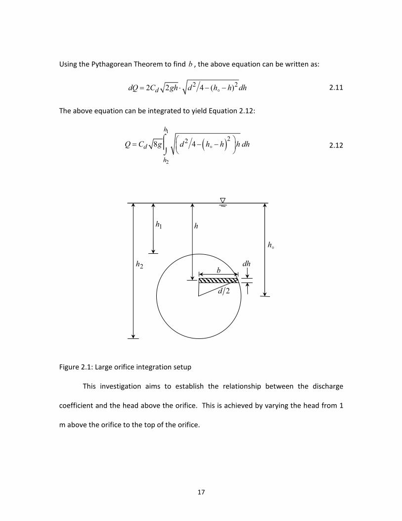
Using the Pythagorean Theorem to find b , the above equation can be written as:
2 22 2 4 ( )ddQ C gh d h h dh= ⋅ − −�
2.11
The above equation can be integrated to yield Equation 2.12:
( )1
2
228 4
h
d
h
Q C g d h h h dh = − −
⌠⌡
� 2.12
Figure 2.1: Large orifice integration setup
This investigation aims to establish the relationship between the discharge
coefficient and the head above the orifice. This is achieved by varying the head from 1
m above the orifice to the top of the orifice.
dh
h�
1h
2h
h
b
2d
18
Effect of orifice height above the floor
As previously discussed, it has been determined that several factors may
influence the value of the discharge coefficient, dC . Among these are the head above
the orifice and the d D ratio. Another potential influencing factor may be the distance
the orifice lies above the bottom of the tank or detention basin. As one side of an
orifice approaches a wall or boundary, the streamlines on that side will gradually
become more parallel to the boundary. This will reduce the amount of contraction the
jet experiences, which means the contraction and discharge coefficients will be higher.
Knowing the effect and the extent of suppression can be useful in determining a
minimum height an orifice should be placed above the floor of the detention basin. This
may be especially useful in design when accounting for the sedimentation rate of a
stormwater basin. As a basin fills with sediment over time, the effective height between
the basin floor and the orifice will decrease. This could lead to an increase in
suppression and therefore an increase in dC . In this investigation, several orifice
heights above the tank floor will be tested to determine the effect of suppression on the
discharge coefficient.
19
CHAPTER 3
EXPERIMENTAL SETUP AND METHODOLOGY
The objective of this experiment was to determine the discharge coefficient for
an orifice cut into the side of a circular pipe, and to determine the effects of pipe
curvature, head above the orifice, and orifice height above the tank floor on the
discharge coefficient. An existing model was adapted and a procedure was developed in
order to accurately determine the discharge coefficient. The procedure for the
experiment utilized a transient method, where a tank was filled with water and allowed
to drain naturally through single and multiple orifices of various sizes cut into risers of
multiple diameters. A pressure transducer was installed to measure the water level in
the tank. A volume-height relationship was developed and used to determine the
change in volume of the tank over time as the water level dropped. This information
was used in the orifice discharge equation to solve for the discharge coefficient, dC .
Physical model setup
The experiment was performed in the hydraulics laboratory of Lowry Hall at
Clemson University in Clemson, SC. The plan and cross-section views of the physical
model are shown in Figures 3.1 and 3.2. The physical model consists of a primary tank
with perforated vertical riser, a secondary discharge basin, and a pump and pipe system
is used to fill the tank to the desired level. The discharge basin collects the outflow from
20
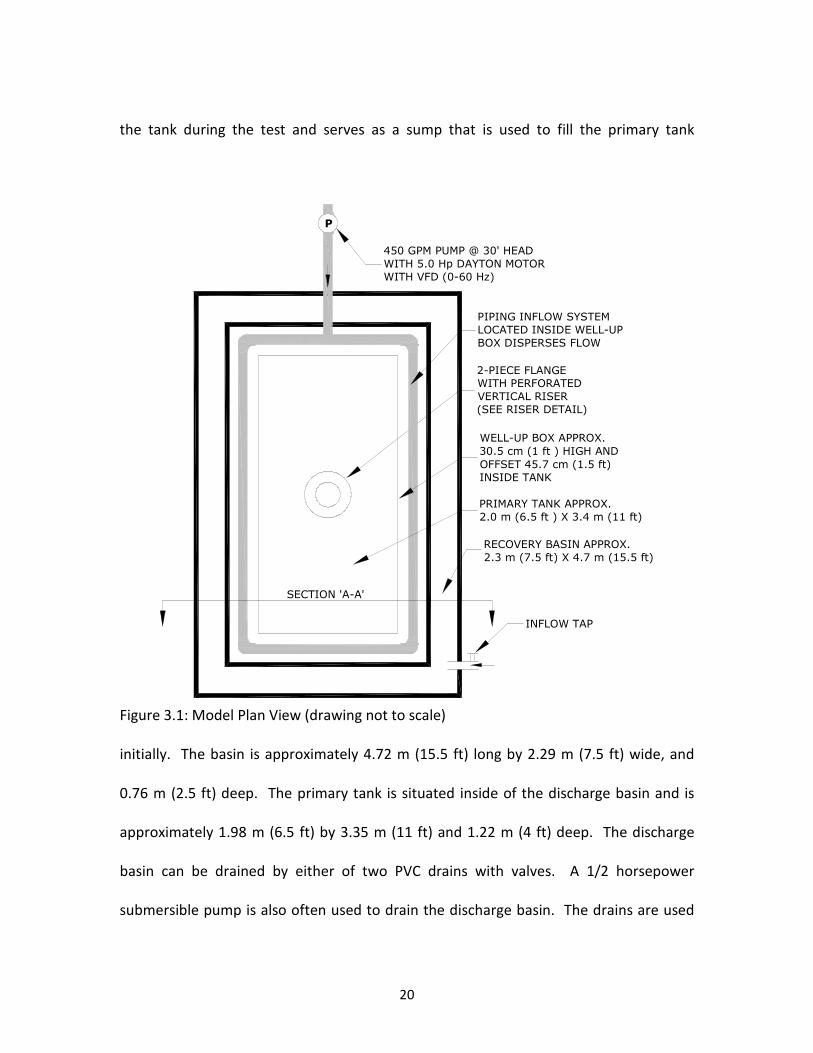
the tank during the test and serves as a sump that is used to fill the primary tank
2-PIECE FLANGE
WITH PERFORATED
VERTICAL RISER
(SEE RISER DETAIL)
Q
WELL-UP BOX APPROX.
30.5 cm (1 ft ) HIGH AND
OFFSET 45.7 cm (1.5 ft)
INSIDE TANK
PRIMARY TANK APPROX.
2.0 m (6.5 ft ) X 3.4 m (11 ft)
RECOVERY BASIN APPROX.
2.3 m (7.5 ft) X 4.7 m (15.5 ft)
PIPING INFLOW SYSTEM
LOCATED INSIDE WELL-UP
BOX DISPERSES FLOW
P
450 GPM PUMP @ 30' HEAD
WITH 5.0 Hp DAYTON MOTOR
WITH VFD (0-60 Hz)
SECTION 'A-A'
INFLOW TAP
Figure 3.1: Model Plan View (drawing not to scale)
initially. The basin is approximately 4.72 m (15.5 ft) long by 2.29 m (7.5 ft) wide, and
0.76 m (2.5 ft) deep. The primary tank is situated inside of the discharge basin and is
approximately 1.98 m (6.5 ft) by 3.35 m (11 ft) and 1.22 m (4 ft) deep. The discharge
basin can be drained by either of two PVC drains with valves. A 1/2 horsepower
submersible pump is also often used to drain the discharge basin. The drains are used
21
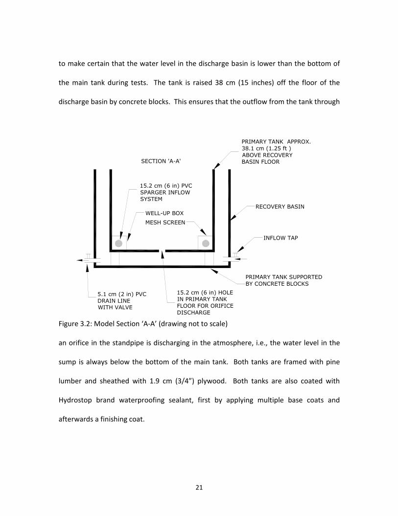
to make certain that the water level in the discharge basin is lower than the bottom of
the main tank during tests. The tank is raised 38 cm (15 inches) off the floor of the
discharge basin by concrete blocks. This ensures that the outflow from the tank through
SECTION 'A-A'
RECOVERY BASIN
PRIMARY TANK APPROX.
38.1 cm (1.25 ft )
ABOVE RECOVERY
BASIN FLOOR
WELL-UP BOX
15.2 cm (6 in) PVC
SPARGER INFLOW
SYSTEM
PRIMARY TANK SUPPORTED
BY CONCRETE BLOCKS
5.1 cm (2 in) PVC
DRAIN LINE
WITH VALVE
15.2 cm (6 in) HOLE
IN PRIMARY TANK
FLOOR FOR ORIFICE
DISCHARGE
MESH SCREEN
INFLOW TAP
Figure 3.2: Model Section ‘A-A’ (drawing not to scale)
an orifice in the standpipe is discharging in the atmosphere, i.e., the water level in the
sump is always below the bottom of the main tank. Both tanks are framed with pine
lumber and sheathed with 1.9 cm (3/4”) plywood. Both tanks are also coated with
Hydrostop brand waterproofing sealant, first by applying multiple base coats and
afterwards a finishing coat.
22
The main tank is filled using a pump and a perforated pipe (sparger) system as
shown in Figures 3.1 and 3.2. The sparger is laid along the perimeter at the bottom of
the tank and forms a closed loop. The holes in the sparger point toward the bed to
minimize the disturbances caused by the inflow in the tank. A well-up box surrounds
the sparger and is covered with fine mesh at the top to further dissipate the inflow
velocities and turbulence.
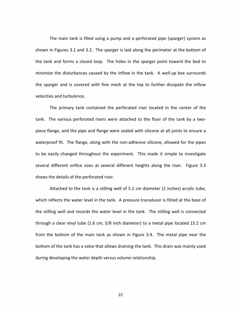
The primary tank contained the perforated riser located in the center of the
tank. The various perforated risers were attached to the floor of the tank by a two-
piece flange, and the pipe and flange were sealed with silicone at all joints to ensure a
waterproof fit. The flange, along with the non-adhesive silicone, allowed for the pipes
to be easily changed throughout the experiment. This made it simple to investigate
several different orifice sizes at several different heights along the riser. Figure 3.3
shows the details of the perforated riser.
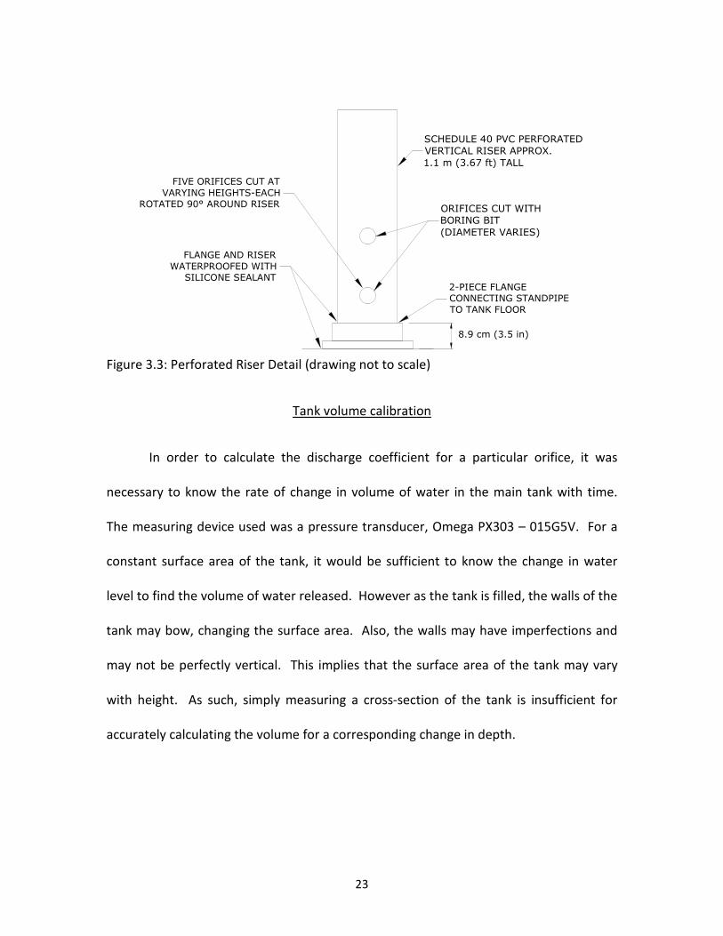
Attached to the tank is a stilling well of 5.1 cm diameter (2 inches) acrylic tube,
which reflects the water level in the tank. A pressure transducer is fitted at the base of
the stilling well and records the water level in the tank. The stilling well is connected
through a clear vinyl tube (1.6 cm, 5/8 inch diameter) to a metal pipe located 15.2 cm
from the bottom of the main tank as shown in Figure 3.4. The metal pipe near the
bottom of the tank has a valve that allows draining the tank. This drain was mainly used
during developing the water depth versus volume relationship.
23
ORIFICES CUT WITH
BORING BIT
(DIAMETER VARIES)
2-PIECE FLANGE
CONNECTING STANDPIPE
TO TANK FLOOR
SCHEDULE 40 PVC PERFORATED
VERTICAL RISER APPROX.
1.1 m (3.67 ft) TALL
FLANGE AND RISER
WATERPROOFED WITH
SILICONE SEALANT
FIVE ORIFICES CUT AT
VARYING HEIGHTS-EACH
ROTATED 90° AROUND RISER
8.9 cm (3.5 in)
Figure 3.3: Perforated Riser Detail (drawing not to scale)
Tank volume calibration
In order to calculate the discharge coefficient for a particular orifice, it was
necessary to know the rate of change in volume of water in the main tank with time.
The measuring device used was a pressure transducer, Omega PX303 – 015G5V. For a
constant surface area of the tank, it would be sufficient to know the change in water
level to find the volume of water released. However as the tank is filled, the walls of the
tank may bow, changing the surface area. Also, the walls may have imperfections and
may not be perfectly vertical. This implies that the surface area of the tank may vary
with height. As such, simply measuring a cross-section of the tank is insufficient for
accurately calculating the volume for a corresponding change in depth.
24
TANK WALL
STILLING BASIN OF
5.1 cm (2 in)
DIAMETER ACRYLIC
1.6 cm (5/8 in)
VINYL TUBING1.3 cm (1/2 in)
METAL PIPE
1.6 cm (5/8 in)
VINYL TUBING DRAIN
WITH VALVE
OMEGA PRESSUER
TRANSDUCER PX303
(TO COMPUTER)
Figure 3.4: Stilling Well Detail (drawing not to scale)
To determine volume versus depth relationship, the tank was filled up to the fill
line (1.1 m from the bottom of the tank). The fill line marks the zero-volume-drained
point. The water was drawn in 18.9 liters (5 gallons) increments from the tank and the
corresponding change in water depth was recorded using the pressure transducer. The
pressure transducer outputs voltage based on the water depth above it and has a linear
relationship between voltage and pressure. The output voltage range is 0.5 to 5.5 volts
with a gauge pressure range of 0 to 103.42 kPa (15 psig). The accuracy of the transducer
as determined by the manufacturer is 0.25% of the full scale.
25
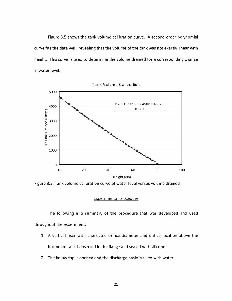
Figure 3.5 shows the tank volume calibration curve. A second-order polynomial
curve fits the data well, revealing that the volume of the tank was not exactly linear with
height. This curve is used to determine the volume drained for a corresponding change
in water level.
T ank Volume C alibration
y = 0.1037x2 - 65.458x + 4657.6
R2 = 1
0
1000
2000
3000
4000
5000
0 20 40 60 80 100
Height (cm)
Vo
lum
e D
rain
ed
(L
ite
rs)
Figure 3.5: Tank volume calibration curve of water level versus volume drained
Experimental procedure
The following is a summary of the procedure that was developed and used
throughout the experiment.
1. A vertical riser with a selected orifice diameter and orifice location above the
bottom of tank is inserted in the flange and sealed with silicone.
2. The inflow tap is opened and the discharge basin is filled with water.
26
3. Once the discharge basin is sufficiently full, the pump is started, and the valve
leading to the primary tank is opened. The main tank begins filling with water.
4. As the water level in the main tank approaches the fill line (1.1 m), the inflow to
the discharge basin is cut off. This helps in keeping the water level in the
discharge basin well below the bottom of the main tank.
5. When the water level in the head tank reaches above the fill line, the LabView
program is started. The inflow to the main tank is cut off immediately and the
pump is stopped. The tank drains through the orifice and water level versus time
data is recorded using the LabView program.
At this point, the tank is freely discharging with no inflow from the pump. The tank is
filled above the fill line to ensure that disturbances caused by the inflow are dissipated
by the time the water level reaches the fill line. Dye tests showed that there were no
secondary flow patterns in the tank and the flow existed only around the orifice. By the
time the water level reaches the zero-volume drained mark, the system is in equilibrium
and the test results are recorded.
Scope of this study
This aim of this study is to investigate the effect of several factors on the
discharge coefficient for orifices cut into thin-walled pipes. The study will use vertical
perforated riser pipes of two different diameters, 15.2 cm (6 in) and 30.5 cm (12 in).
The 15.cm riser has a pipe wall thickness of 7.7 mm and the 30.5 cm riser has a wall
27
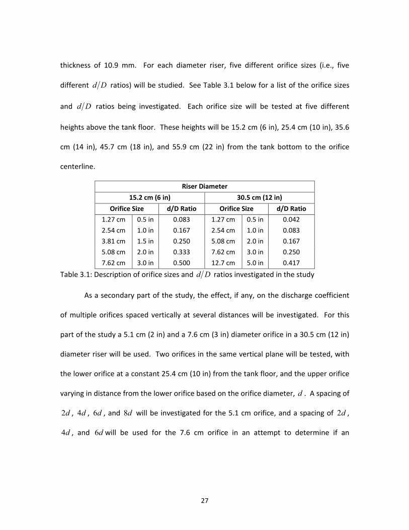
thickness of 10.9 mm. For each diameter riser, five different orifice sizes (i.e., five
different d D ratios) will be studied. See Table 3.1 below for a list of the orifice sizes
and d D ratios being investigated. Each orifice size will be tested at five different
heights above the tank floor. These heights will be 15.2 cm (6 in), 25.4 cm (10 in), 35.6
cm (14 in), 45.7 cm (18 in), and 55.9 cm (22 in) from the tank bottom to the orifice
centerline.
Riser Diameter
15.2 cm (6 in) 30.5 cm (12 in)
Orifice Size d/D Ratio Orifice Size d/D Ratio
1.27 cm 0.5 in 0.083 1.27 cm 0.5 in 0.042
2.54 cm 1.0 in 0.167 2.54 cm 1.0 in 0.083
3.81 cm 1.5 in 0.250 5.08 cm 2.0 in 0.167
5.08 cm 2.0 in 0.333 7.62 cm 3.0 in 0.250
7.62 cm 3.0 in 0.500 12.7 cm 5.0 in 0.417
Table 3.1: Description of orifice sizes and d D ratios investigated in the study
As a secondary part of the study, the effect, if any, on the discharge coefficient
of multiple orifices spaced vertically at several distances will be investigated. For this
part of the study a 5.1 cm (2 in) and a 7.6 cm (3 in) diameter orifice in a 30.5 cm (12 in)
diameter riser will be used. Two orifices in the same vertical plane will be tested, with
the lower orifice at a constant 25.4 cm (10 in) from the tank floor, and the upper orifice
varying in distance from the lower orifice based on the orifice diameter, d . A spacing of
2d , 4d , 6d , and 8d will be investigated for the 5.1 cm orifice, and a spacing of 2d ,
4d , and 6d will be used for the 7.6 cm orifice in an attempt to determine if an
28
interaction of the flow between the orifices causes a reduction in the discharge
coefficient.
29
CHAPTER 4
ANALYTICAL PROCEDURE
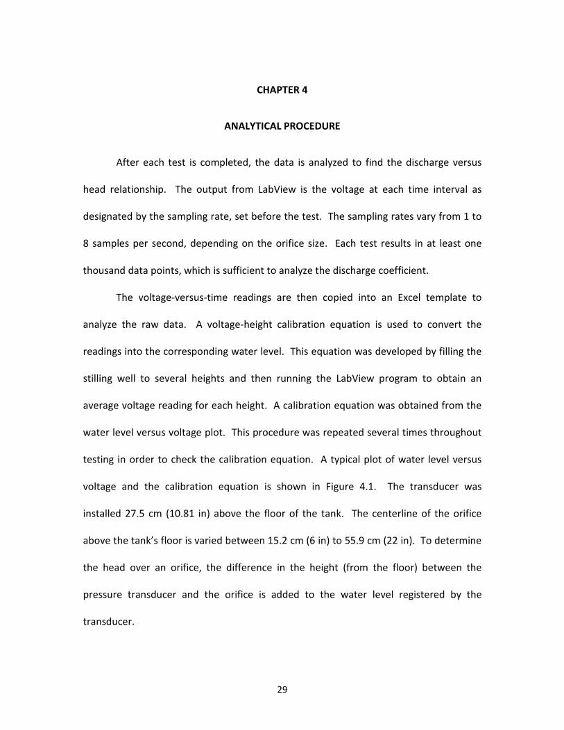
After each test is completed, the data is analyzed to find the discharge versus
head relationship. The output from LabView is the voltage at each time interval as
designated by the sampling rate, set before the test. The sampling rates vary from 1 to
8 samples per second, depending on the orifice size. Each test results in at least one
thousand data points, which is sufficient to analyze the discharge coefficient.
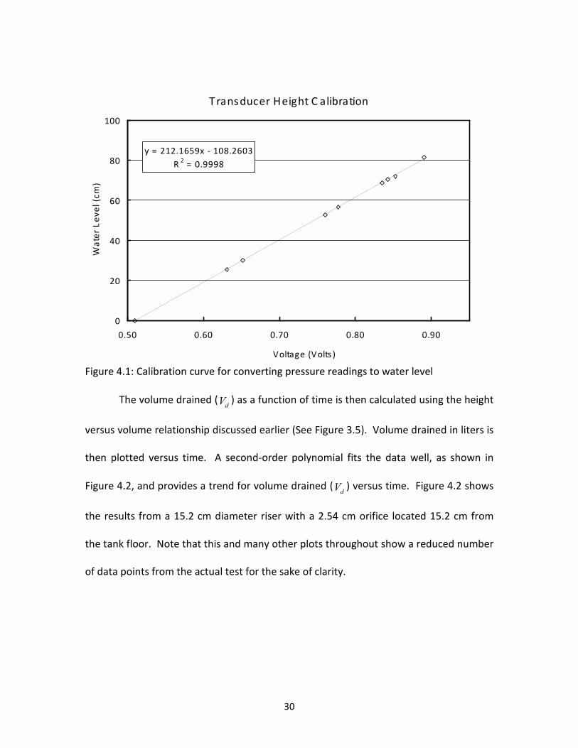
The voltage-versus-time readings are then copied into an Excel template to
analyze the raw data. A voltage-height calibration equation is used to convert the
readings into the corresponding water level. This equation was developed by filling the
stilling well to several heights and then running the LabView program to obtain an
average voltage reading for each height. A calibration equation was obtained from the
water level versus voltage plot. This procedure was repeated several times throughout
testing in order to check the calibration equation. A typical plot of water level versus
voltage and the calibration equation is shown in Figure 4.1. The transducer was
installed 27.5 cm (10.81 in) above the floor of the tank. The centerline of the orifice
above the tank’s floor is varied between 15.2 cm (6 in) to 55.9 cm (22 in). To determine
the head over an orifice, the difference in the height (from the floor) between the
pressure transducer and the orifice is added to the water level registered by the
transducer.
30
T ransducer Height C alibration
y = 212.1659x - 108.2603
R2 = 0.9998
0
20
40
60
80
100
0.50 0.60 0.70 0.80 0.90
Voltage (Volts )
Wa
ter
Le
ve
l (c
m)
Figure 4.1: Calibration curve for converting pressure readings to water level
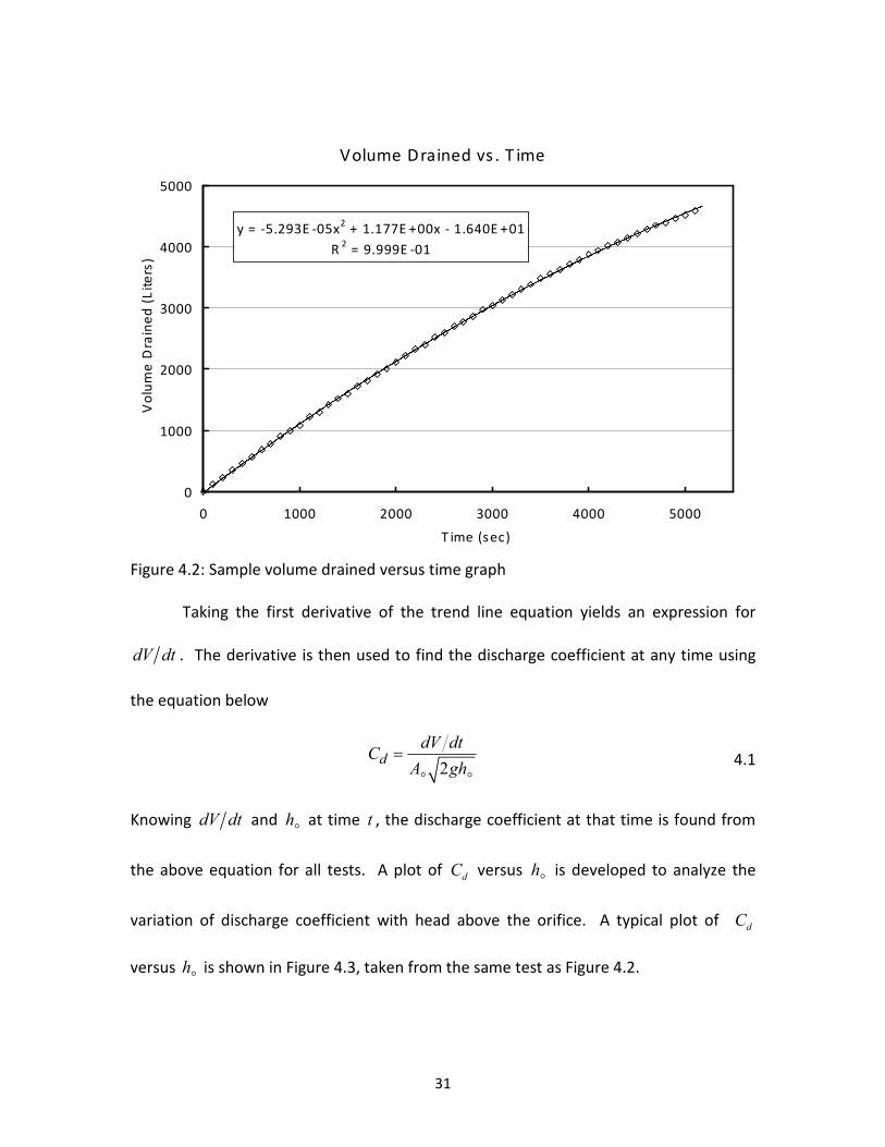
The volume drained (dV ) as a function of time is then calculated using the height
versus volume relationship discussed earlier (See Figure 3.5). Volume drained in liters is
then plotted versus time. A second-order polynomial fits the data well, as shown in
Figure 4.2, and provides a trend for volume drained (dV ) versus time. Figure 4.2 shows
the results from a 15.2 cm diameter riser with a 2.54 cm orifice located 15.2 cm from
the tank floor. Note that this and many other plots throughout show a reduced number
of data points from the actual test for the sake of clarity.
31
Volume Drained vs . T ime
y = -5.293E -05x2 + 1.177E +00x - 1.640E +01
R2 = 9.999E -01
0
1000
2000
3000
4000
5000
0 1000 2000 3000 4000 5000
T ime (sec)
Vo
lum
e D
rain
ed
(L
ite
rs)
Figure 4.2: Sample volume drained versus time graph
Taking the first derivative of the trend line equation yields an expression for
dV dt . The derivative is then used to find the discharge coefficient at any time using
the equation below
2d
dV dtC
A gh=� �
4.1
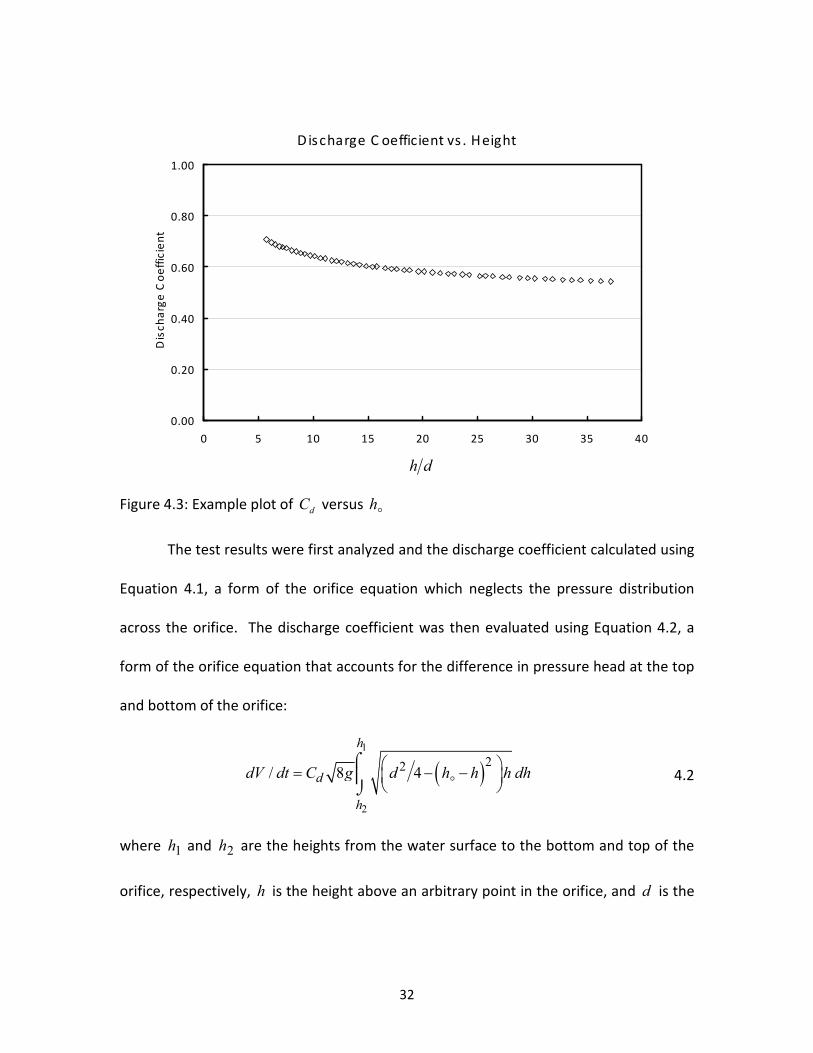
Knowing dV dt and h�
at time t , the discharge coefficient at that time is found from
the above equation for all tests. A plot of dC versus h�
is developed to analyze the
variation of discharge coefficient with head above the orifice. A typical plot of dC
versus h�
is shown in Figure 4.3, taken from the same test as Figure 4.2.
32
Discharge C oefficient vs . Height
0.00
0.20
0.40
0.60
0.80
1.00
0 5 10 15 20 25 30 35 40
Dis
ch
arg
e C
oe
ffic
ien
t
Figure 4.3: Example plot of dC versus h�
The test results were first analyzed and the discharge coefficient calculated using
Equation 4.1, a form of the orifice equation which neglects the pressure distribution
across the orifice. The discharge coefficient was then evaluated using Equation 4.2, a
form of the orifice equation that accounts for the difference in pressure head at the top
and bottom of the orifice:
( )1
2
22/ 8 4
h
d
h
dV dt C g d h h h dh = − −
⌠⌡
� 4.2
where 1h and 2h are the heights from the water surface to the bottom and top of the
orifice, respectively, h is the height above an arbitrary point in the orifice, and d is the
h d
33
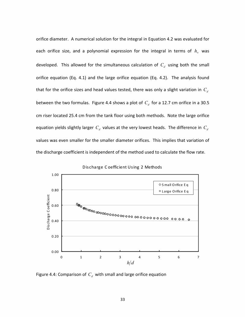
orifice diameter. A numerical solution for the integral in Equation 4.2 was evaluated for
each orifice size, and a polynomial expression for the integral in terms of h�
was
developed. This allowed for the simultaneous calculation of dC using both the small
orifice equation (Eq. 4.1) and the large orifice equation (Eq. 4.2). The analysis found
that for the orifice sizes and head values tested, there was only a slight variation in dC
between the two formulas. Figure 4.4 shows a plot of dC for a 12.7 cm orifice in a 30.5
cm riser located 25.4 cm from the tank floor using both methods. Note the large orifice
equation yields slightly larger dC values at the very lowest heads. The difference in dC
values was even smaller for the smaller diameter orifices. This implies that variation of
the discharge coefficient is independent of the method used to calculate the flow rate.
Discharge C oefficient Us ing 2 Methods
0.00
0.20
0.40
0.60
0.80
1.00
0 1 2 3 4 5 6 7
Dis
ch
arg
e C
oe
ffic
ien
t
S mall O rifice E q
L arge Orifice E q
Figure 4.4: Comparison of dC with small and large orifice equation
h d
34
CHAPTER 5
TEST RESULTS
The primary study focused on the effect of d D ratio, orifice height from the
floor, and the head above the orifice on the discharge coefficient. The secondary
portion of this study tested the influence of spacing on discharge coefficient for multiple
orifices. The primary study utilized two different sizes of standpipes having diameter of
15.2 cm (6 in) and 30.5 cm (12 in) and five different sizes of orifices as shown in Table
3.1. Each orifice size in a given riser pipe was tested at five different locations above the
floor of the tank (details given in Chapter 3). For each orifice size, at least one of the
tests was run multiple times to ensure repeatability.
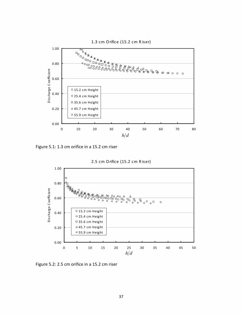
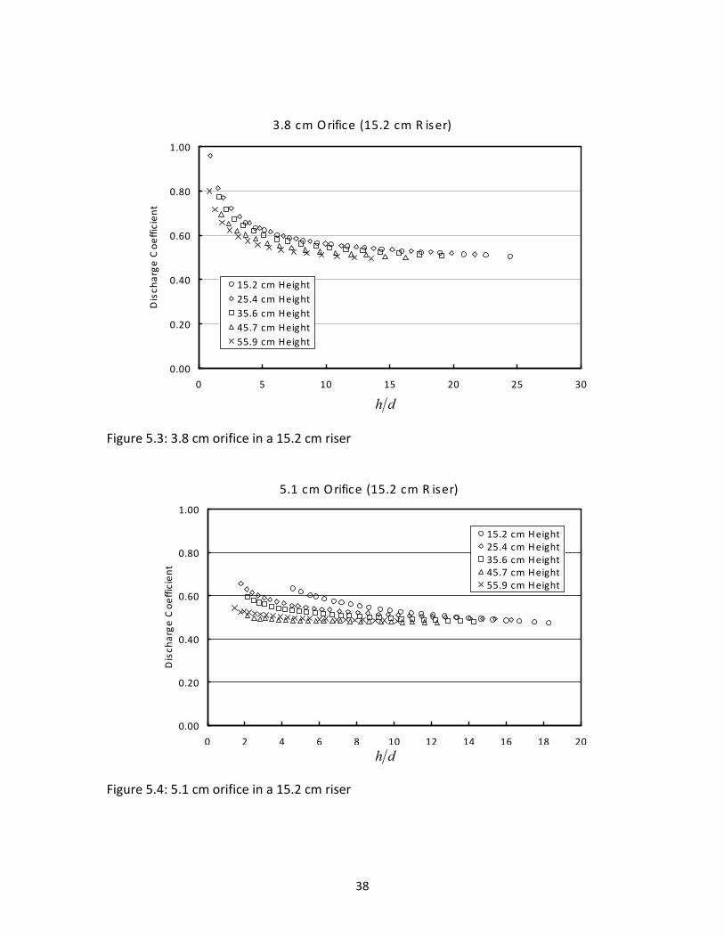
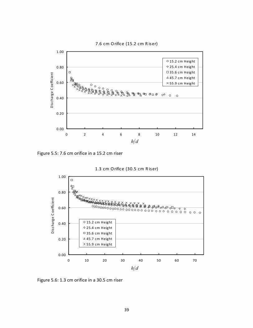
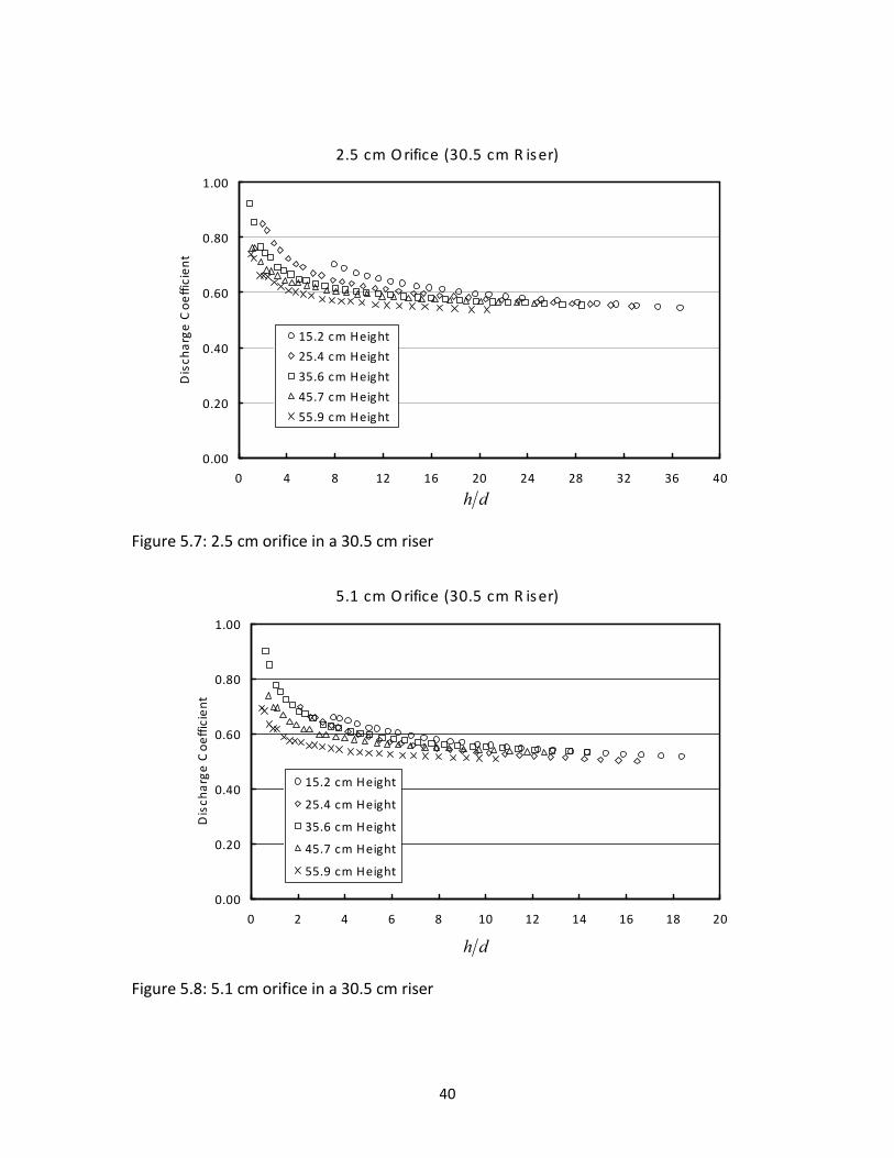
Figures 5.1 – 5.10 were normalized by dividing the water level height by the
orifice size (h d ), which was constant in each plot. Figures 5.11 – 5.20 contained all
different orifice sizes in each plot, so the length scale was normalized by dividing the
water level by the riser diameter (h D ), which was constant for each plot. Normalizing
these figures by orifice size would have led to different length scales in each plot, and
made it difficult to view trends in the data. As noted in Chapter 3, all figures shown
have reduced data points for clarity in viewing the test results.
35
Effect of the head above the orifice
Figures 5.1 – 5.20 show the compiled data for both riser diameters and all orifice
heights and sizes. As the same method was utilized for each test, each plot shows the
effect of changing head values on the discharge coefficient. The most noticeable
characteristic of these plots is that for a given orifice size the dC increases as the head
decreases. This phenomenon was observed with every orifice size at every floor height
for both risers. For most cases, the increase in dC became more drastic as head values
approached the top of the orifice. This is expected as the velocity exiting the orifice
reduces with decreasing head over the orifice. As head decreases, flow streamlines
approach the orifice at increasingly lower velocities. This leads to an increase in the
area of the jet at the vena contracta and an increase in the contraction coefficient, cC .
Since the discharge coefficient is influenced by the contraction coefficient, any increase
in cC will increase dC . In addition, for a given orifice size, the discharge coefficient
reaches a constant value at high head values.
Effect of orifice height above the floor
The influence of the orifice height above the floor on the discharge coefficient is
shown in Figures 5.1 – 5.10. Each figure shows test results for a given orifice size and
riser pipe at all locations above the floor of the tank. The data show that location
effects are less pronounced at higher head values. The figures also show that the
36
discharge coefficient decreases with the increase in the height of the orifice from the
floor. This is consistent with the notion discussed in Chapter 2 that an orifice may
experience suppression of the jet contraction as it approaches a boundary. The
boundary may force the flow streamlines to enter the orifice at increasingly normal
angles, resulting in less contraction of the jet. The exceptions to this trend can be seen
with a 1.3 cm and 2.5 cm orifice in the 15.2 cm diameter riser (Figures 5.1 and 5.2) and
with a 1.3 cm orifice in the 30.5 cm riser (Figure 5.6). These were cases of the smallest
orifice sizes and d D ratios investigated. One explanation for the discrepancy could be
that the area from which an orifice draws its flow increases with orifice size, and the
flow field for these orifices may not have interacted with the floor of the tank. It may be
that the orifices would experience an increase in dC if they were located much closer to
the floor of the tank. However, the flange used to install the riser pipes prevented tests
from being run at heights lower than 15.2 cm.
It can also be noted from Figures 5.1 – 5.10 that for a given orifice the discharge
coefficient tends to become independent of the orifice’s location as the height of the
orifice above the floor increases. The dC curves for locations of 45.7 cm and 55.9 cm
above the floor are nearly the same. These two orifice heights were further analyzed
and are discussed later.
37
1.3 cm O rifice (15.2 cm R iser)
0.00
0.20
0.40
0.60
0.80
1.00
0 10 20 30 40 50 60 70 80
Dis
ch
arg
e C
oe
ffic
ien
t
15.2 cm Height
25.4 cm Height
35.6 cm Height
45.7 cm Height
55.9 cm Height
Figure 5.1: 1.3 cm orifice in a 15.2 cm riser
2.5 cm O rifice (15.2 cm R iser)
0.00
0.20
0.40
0.60
0.80
1.00
0 5 10 15 20 25 30 35 40 45 50
Dis
ch
arg
e C
oe
ffic
ien
t
15.2 cm Height
25.4 cm Height
35.6 cm Height
45.7 cm Height
55.9 cm Height
Figure 5.2: 2.5 cm orifice in a 15.2 cm riser
h d
h d
38
3.8 cm Orifice (15.2 cm R iser)
0.00
0.20
0.40
0.60
0.80
1.00
0 5 10 15 20 25 30
Dis
ch
arg
e C
oe
ffic
ien
t
15.2 cm Height
25.4 cm Height
35.6 cm Height
45.7 cm Height
55.9 cm Height
Figure 5.3: 3.8 cm orifice in a 15.2 cm riser
5.1 cm Orifice (15.2 cm R iser)
0.00
0.20
0.40
0.60
0.80
1.00
0 2 4 6 8 10 12 14 16 18 20
Dis
ch
arg
e C
oe
ffic
ien
t
15.2 cm Height
25.4 cm Height
35.6 cm Height
45.7 cm Height
55.9 cm Height
Figure 5.4: 5.1 cm orifice in a 15.2 cm riser
h d
h d
39
7.6 cm O rifice (15.2 cm R iser)
0.00
0.20
0.40
0.60
0.80
1.00
0 2 4 6 8 10 12 14
Dis
ch
arg
e C
oe
ffic
ien
t
15.2 cm Height
25.4 cm Height
35.6 cm Height
45.7 cm Height
55.9 cm Height
Figure 5.5: 7.6 cm orifice in a 15.2 cm riser
1.3 cm O rifice (30.5 cm R iser)
0.00
0.20
0.40
0.60
0.80
1.00
0 10 20 30 40 50 60 70
Dis
ch
arg
e C
oe
ffic
ien
t
15.2 cm Height
25.4 cm Height
35.6 cm Height
45.7 cm Height
55.9 cm Height
Figure 5.6: 1.3 cm orifice in a 30.5 cm riser
h d
h d
40
2.5 cm O rifice (30.5 cm R iser)
0.00
0.20
0.40
0.60
0.80
1.00
0 4 8 12 16 20 24 28 32 36 40
Dis
ch
arg
e C
oe
ffic
ien
t
15.2 cm Height
25.4 cm Height
35.6 cm Height
45.7 cm Height
55.9 cm Height
Figure 5.7: 2.5 cm orifice in a 30.5 cm riser
5.1 cm O rifice (30.5 cm R iser)
0.00
0.20
0.40
0.60
0.80
1.00
0 2 4 6 8 10 12 14 16 18 20
Dis
ch
arg
e C
oe
ffic
ien
t
15.2 cm Height
25.4 cm Height
35.6 cm Height
45.7 cm Height
55.9 cm Height
Figure 5.8: 5.1 cm orifice in a 30.5 cm riser
h d
h d
41
7.6 cm O rifice (30.5 cm R iser)
0.00
0.20
0.40
0.60
0.80
1.00
0 1 2 3 4 5 6 7 8 9 10 11 12 13 14 15
Dis
ch
arg
e C
oe
ffic
ien
t
15.2 cm Height
25.4 cm Height
35.6 cm Height
45.7 cm Height
55.9 cm Height
Figure 5.9: 7.6 cm orifice in a 30.5 cm riser
12.7 cm Orifice (30.5 cm R iser)
0.00
0.20
0.40
0.60
0.80
1.00
0 1 2 3 4 5 6 7 8 9 10
Dis
ch
arg
e C
oe
ffic
ien
t
15.2 cm Height
25.4 cm Height
35.6 cm Height
45.7 cm Height
55.9 cm Height
Figure 5.10: 12.7 cm orifice in a 30.5 cm riser
h d
h d
42
Figures 5.1 through 5.10 show the effect of height above the floor on the
discharge coefficient for various size orifices. It is apparent that in most cases as the
height from the floor is increased, dC is decreased until the 45.7 cm height, at which
point the discharge coefficients are no longer affected by the tank floor. Further
analysis was done in order to determine if the floor height to orifice diameter ratio
( fh d ) plays a role in whether the discharge coefficient will be affected. However, no
discernable trends could be found from the limited data of constant floor height to
orifice diameter ratio.
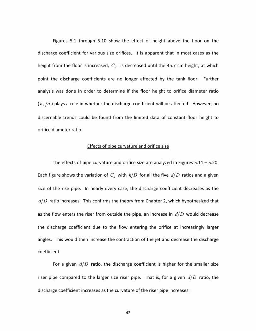
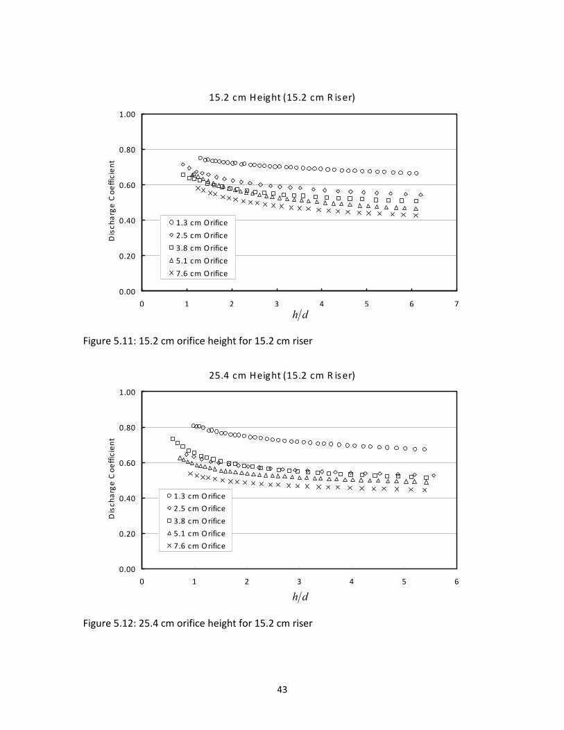
Effects of pipe curvature and orifice size
The effects of pipe curvature and orifice size are analyzed in Figures 5.11 – 5.20.
Each figure shows the variation of dC with h D for all the five d D ratios and a given
size of the rise pipe. In nearly every case, the discharge coefficient decreases as the
d D ratio increases. This confirms the theory from Chapter 2, which hypothesized that
as the flow enters the riser from outside the pipe, an increase in d D would decrease
the discharge coefficient due to the flow entering the orifice at increasingly larger
angles. This would then increase the contraction of the jet and decrease the discharge
coefficient.
For a given d D ratio, the discharge coefficient is higher for the smaller size
riser pipe compared to the larger size riser pipe. That is, for a given d D ratio, the
discharge coefficient increases as the curvature of the riser pipe increases.
43
15.2 cm Height (15.2 cm R iser)
0.00
0.20
0.40
0.60
0.80
1.00
0 1 2 3 4 5 6 7
Dis
ch
arg
e C
oe
ffic
ien
t
1.3 cm Orifice
2.5 cm Orifice
3.8 cm Orifice
5.1 cm Orifice
7.6 cm Orifice
Figure 5.11: 15.2 cm orifice height for 15.2 cm riser
25.4 cm Height (15.2 cm R iser)
0.00
0.20
0.40
0.60
0.80
1.00
0 1 2 3 4 5 6
Dis
ch
arg
e C
oe
ffic
ien
t
1.3 cm Orifice
2.5 cm Orifice
3.8 cm Orifice
5.1 cm Orifice
7.6 cm Orifice
Figure 5.12: 25.4 cm orifice height for 15.2 cm riser
h d
h d
44
35.6 cm Height (15.2 cm R iser)
0.00
0.20
0.40
0.60
0.80
1.00
0 1 2 3 4 5 6
Dis
ch
arg
e C
oe
ffic
ien
t
1.3 cm Orifice
2.5 cm Orifice
3.8 cm Orifice
5.1 cm Orifice
7.6 cm Orifice
Figure 5.13: 35.6 cm orifice height for 15.2 cm riser
45.7 cm Height (15.2 cm R iser)
0.00
0.20
0.40
0.60
0.80
1.00
0 1 2 3 4 5
Dis
ch
arg
e C
oe
ffic
ien
t
1.3 cm Orifice
2.5 cm Orifice
3.8 cm Orifice
5.1 cm Orifice
7.6 cm Orifice
Figure 5.14: 45.7 cm orifice height for 15.2 cm riser
h d
h d
45
55.9 cm Height (15.2 cm R iser)
0.00
0.20
0.40
0.60
0.80
1.00
0 1 2 3 4
Dis
ch
arg
e C
oe
ffic
ien
t
1.3 cm O rifice
2.5 cm O rifice
3.8 cm O rifice
5.1 cm O rifice
7.6 cm O rifice
Figure 5.15: 55.9 cm orifice height for 15.2 cm riser
15.2 cm Height (30.5 cm R iser)
0.00
0.20
0.40
0.60
0.80
1.00
0 0.5 1 1.5 2 2.5 3 3.5
Dis
ch
arg
e C
oe
ffic
ien
t
1.3 cm Orifice
2.5 cm Orifice
5.1 cm Orifice
7.6 cm Orifice
12.7 cm Orifice
Figure 5.16: 15.2 cm orifice height for 30.5 cm riser
h d
h d
46
25.4 cm Height (30.5 cm R iser)
0.00
0.20
0.40
0.60
0.80
1.00
0 0.5 1 1.5 2 2.5 3
Dis
ch
arg
e C
oe
ffic
ien
t
1.3 cm Orifice
2.5 cm Orifice
5.1 cm Orifice
7.6 cm Orifice
12.7 cm Orifice
Figure 5.17: 25.4 cm orifice height for 30.5 cm riser
35.6 cm Height (30.5 cm R iser)
0.00
0.20
0.40
0.60
0.80
1.00
0 0.5 1 1.5 2 2.5 3
Dis
ch
arg
e C
oe
ffic
ien
t
1.3 cm Orifice 2.5 cm Orifice
5.1 cm Orifice 7.6 cm Orifice
12.7 cm Orifice
Figure 5.18: 35.6 cm orifice height for 30.5 cm riser
h d
h d
47
45.7 cm Height (30.5 cm R iser)
0.00
0.20
0.40
0.60
0.80
1.00
0 0.5 1 1.5 2 2.5
Dis
ch
arg
e C
oe
ffic
ien
t
1.3 cm Orifice 2.5 cm Orifice
5.1 cm Orifice 7.6 cm Orifice
12.7 cm Orifice
Figure 5.19: 45.7 cm orifice height for 30.5 cm riser
55.9 cm Height (30.5 cm R iser)
0.00
0.20
0.40
0.60
0.80
1.00
0 0.5 1 1.5 2
Dis
ch
arg
e C
oe
ffic
ien
t
1.3 cm Orifice 2.5 cm Orifice
5.1 cm Orifice 7.6 cm Orifice
12.7 cm Orifice
Figure 5.20: 55.9 cm orifice height for 30.5 cm riser
h d
h d
48
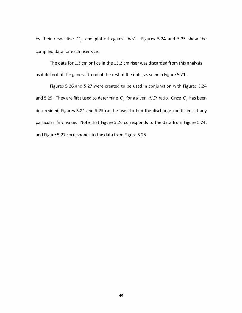
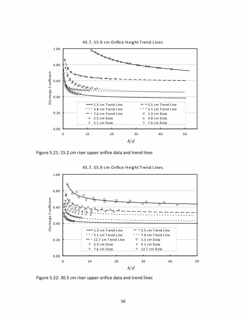
Combination of height-independent data
Noting that the first analysis of the test results showed that the two upper-most
orifice heights (45.7 cm and 55.9 cm) yielded discharge coefficients that were
independent of the height of the orifice above the floor, data for these orifice heights
were seperated for each orifice size and further analyzed. First, trendlines were
developed for all orifice sizes. Figures 5.21 and 5.22 show these results for the 15.2 cm
riser and the 30.5 cm riser, respectively. The trend lines shown in Figures 5.21 and 5.22
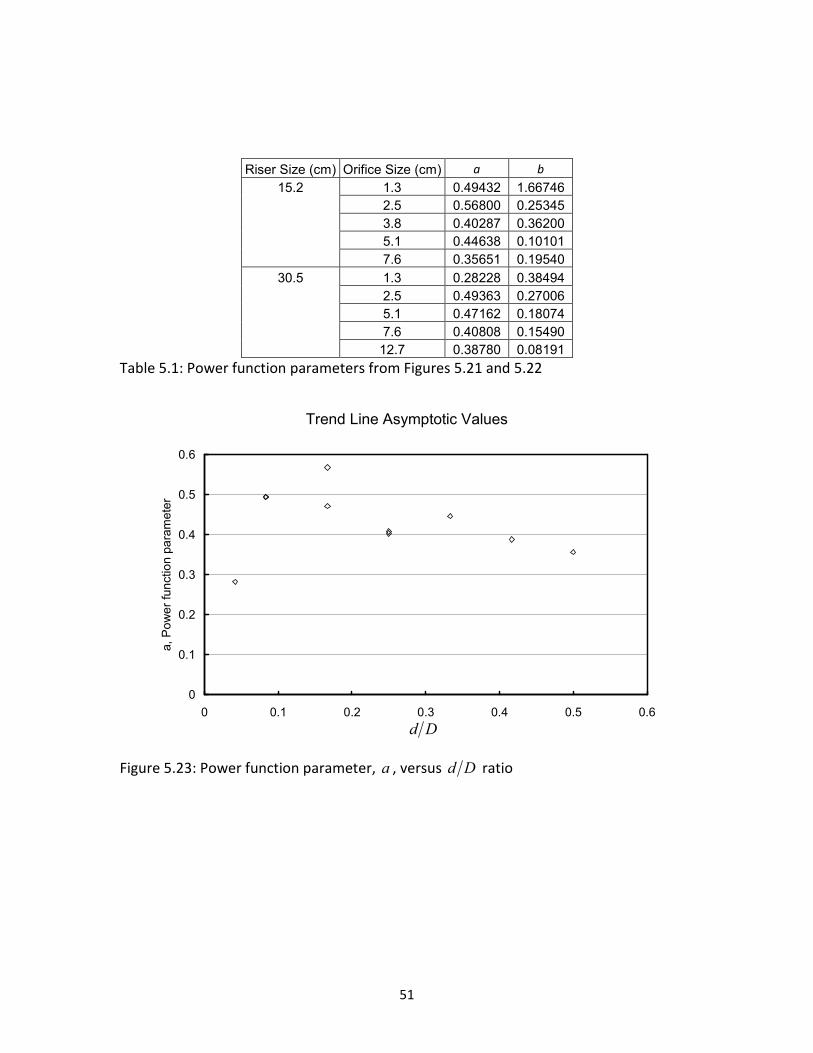
were of the form shown below:
dh
baCd
/+= 5.1
This form of the power equation was chosen because it had high correlation values with
the data. Also the general trend of the data is similar to a plot of 1y x= . Table 5.1
presents values of a and b for both riser diameters and all orifice sizes. Figure 5.23
shows the parameter a plotted versus d D ratio. This plot shows how the asymptotic
value for each trend line varies with pipe curvature. The parameter, a , tends to
decrese with increasing d D ratio.
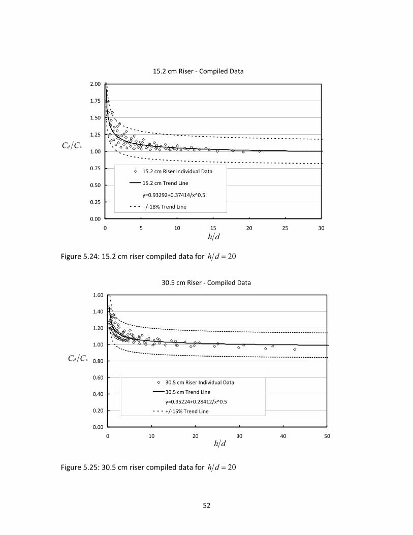
After compiling the data in this fashion, it became apparent that for design
purposes more general equations would be required. To achieve this, an h d value of
20 was chosen, and the discharge coefficient for each orifice at 20h d = was found,
denoted here as oC . The discharge coefficient values for each orifice were then divided
49
by their respective oC , and plotted against h d . Figures 5.24 and 5.25 show the
compiled data for each riser size.
The data for 1.3 cm orifice in the 15.2 cm riser was discarded from this analysis
as it did not fit the general trend of the rest of the data, as seen in Figure 5.21.
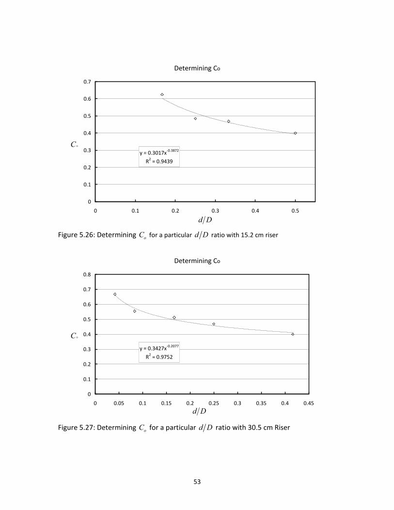
Figures 5.26 and 5.27 were created to be used in conjunction with Figures 5.24
and 5.25. They are first used to determine oC for a given d D ratio. Once oC has been
determined, Figures 5.24 and 5.25 can be used to find the discharge coefficient at any
particular h d value. Note that Figure 5.26 corresponds to the data from Figure 5.24,
and Figure 5.27 corresponds to the data from Figure 5.25.
50
45.7, 55.9 cm Orifice Height T rend L ines
0.00
0.20
0.40
0.60
0.80
1.00
0 10 20 30 40 50
Dis
ch
arg
e C
oe
ffic
ien
t
1.3 cm T rend L ine 2.5 cm T rend L ine
3.8 cm T rend L ine 5.1 cm T rend L ine
7.6 cm T rend L ine 1.3 cm Data
2.5 cm Data 3.8 cm Data
5.1 cm Data 7.6 cm Data
Figure 5.21: 15.2 cm riser upper orifice data and trend lines
45.7, 55.9 cm Orifice Height T rend L ines
0.00
0.20
0.40
0.60
0.80
1.00
0 10 20 30 40 50
Dis
ch
arg
e C
oe
ffic
ien
t
1.3 cm T rend L ine 2.5 cm T rend L ine
5.1 cm T rend L ine 7.6 cm T rend L ine
12.7 cm T rend L ine 1.3 cm Data
2.5 cm Data 5.1 cm Data
7.6 cm Data 12.7 cm Data
Figure 5.22: 30.5 cm riser upper orifice data and trend lines
h d
h d
51
Riser Size (cm) Orifice Size (cm) a b
15.2 1.3 0.49432 1.66746
2.5 0.56800 0.25345
3.8 0.40287 0.36200
5.1 0.44638 0.10101
7.6 0.35651 0.19540
30.5 1.3 0.28228 0.38494
2.5 0.49363 0.27006
5.1 0.47162 0.18074
7.6 0.40808 0.15490
12.7 0.38780 0.08191
Table 5.1: Power function parameters from Figures 5.21 and 5.22
Trend Line Asymptotic Values
0
0.1
0.2
0.3
0.4
0.5
0.6
0 0.1 0.2 0.3 0.4 0.5 0.6
a, Power function parameter
Figure 5.23: Power function parameter, a , versus d D ratio
d D
52
15.2 cm Riser - Compiled Data
0.00
0.25
0.50
0.75
1.00
1.25
1.50
1.75
2.00
0 5 10 15 20 25 30
15.2 cm Riser Individual Data
15.2 cm Trend Line
y=0.93292+0.37414/x^0.5
+/-18% Trend Line
Figure 5.24: 15.2 cm riser compiled data for 20h d =
30.5 cm Riser - Compiled Data
0.00
0.20
0.40
0.60
0.80
1.00
1.20
1.40
1.60
0 10 20 30 40 50
30.5 cm Riser Individual Data
30.5 cm Trend Line
y=0.95224+0.28412/x^0.5
+/-15% Trend Line
Figure 5.25: 30.5 cm riser compiled data for 20h d =
h d
h d
dC C�
dC C�
53
Determining Co
y = 0.3017x-0.3872
R2 = 0.9439
0
0.1
0.2
0.3
0.4
0.5
0.6
0.7
0 0.1 0.2 0.3 0.4 0.5
Figure 5.26: Determining oC for a particular d D ratio with 15.2 cm riser
Determining Co
y = 0.3427x-0.2077
R2 = 0.9752
0
0.1
0.2
0.3
0.4
0.5
0.6
0.7
0.8
0 0.05 0.1 0.15 0.2 0.25 0.3 0.35 0.4 0.45
Figure 5.27: Determining oC for a particular d D ratio with 30.5 cm Riser
C�
d D
d D
C�
54
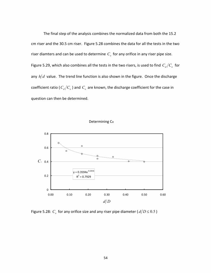
The final step of the analysis combines the normalized data from both the 15.2
cm riser and the 30.5 cm riser. Figure 5.28 combines the data for all the tests in the two
riser diamters and can be used to determine oC for any orifice in any riser pipe size.
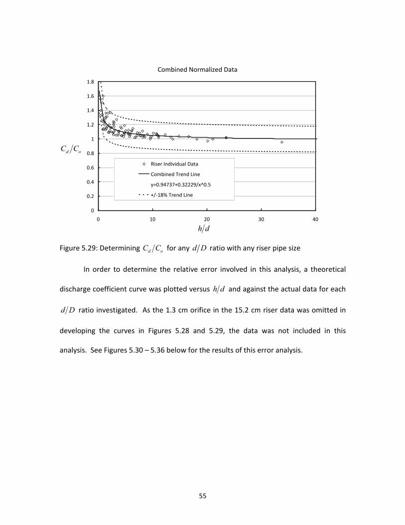
Figure 5.29, which also combines all the tests in the two risers, is used to find d oC C for
any h d value. The trend line function is also shown in the figure. Once the discharge
coefficient ratio ( d oC C ) and oC are known, the discharge coefficient for the case in
question can then be determined.
Determining Co
y = 0.3594x-0.2016
R2 = 0.7929
0
0.2
0.4
0.6
0.8
0.00 0.10 0.20 0.30 0.40 0.50 0.60
Figure 5.28: oC for any orifice size and any riser pipe diameter ( 0.5d D ≤ )
d D
C�
55
Combined Normalized Data
0
0.2
0.4
0.6
0.8
1
1.2
1.4
1.6
1.8
0 10 20 30 40
Riser Individual Data
Combined Trend Line
y=0.94737+0.32229/x^0.5
+/-18% Trend Line
Figure 5.29: Determining d oC C for any d D ratio with any riser pipe size
In order to determine the relative error involved in this analysis, a theoretical
discharge coefficient curve was plotted versus h d and against the actual data for each
d D ratio investigated. As the 1.3 cm orifice in the 15.2 cm riser data was omitted in
developing the curves in Figures 5.28 and 5.29, the data was not included in this
analysis. See Figures 5.30 – 5.36 below for the results of this error analysis.
h d
d oC C
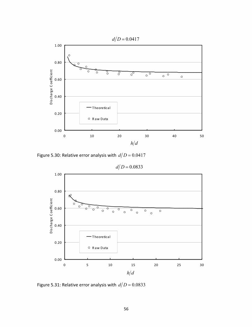
56
0.00
0.20
0.40
0.60
0.80
1.00
0 10 20 30 40 50
Dis
ch
arg
e C
oe
ffic
ien
t
T heoretical
R aw Data
Figure 5.30: Relative error analysis with 0.0417d D =
0.00
0.20
0.40
0.60
0.80
1.00
0 5 10 15 20 25 30
Dis
ch
arg
e C
oe
ffic
ien
t
T heoretical
R aw Data
Figure 5.31: Relative error analysis with 0.0833d D =
h d
0.0417d D =
h d
0.0833d D =
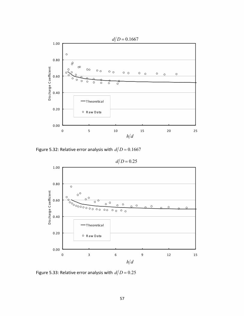
57
0.00
0.20
0.40
0.60
0.80
1.00
0 5 10 15 20 25
Dis
ch
arg
e C
oe
ffic
ien
t
T heoretical
R aw Data
Figure 5.32: Relative error analysis with 0.1667d D =
0.00
0.20
0.40
0.60
0.80
1.00
0 3 6 9 12 15
Dis
ch
arg
e C
oe
ffic
ien
t
T heoretical
R aw Data
Figure 5.33: Relative error analysis with 0.25d D =
h d
h d
0.1667d D =
0.25d D =
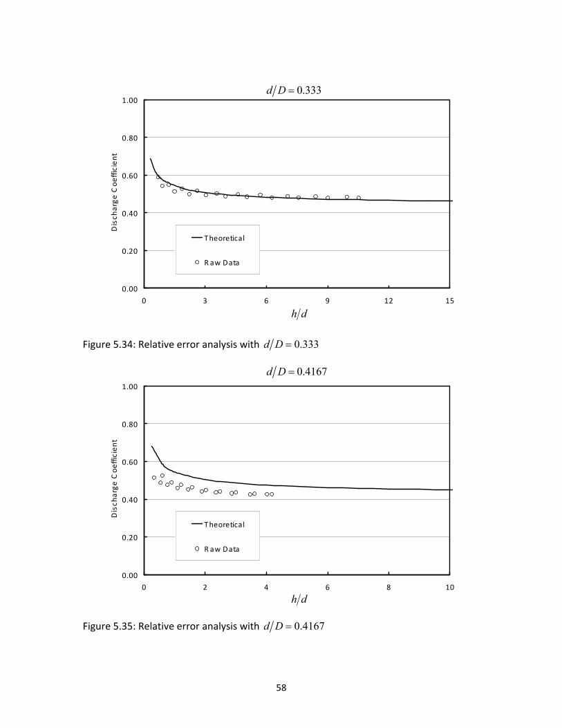
58
0.00
0.20
0.40
0.60
0.80
1.00
0 3 6 9 12 15
Dis
ch
arg
e C
oe
ffic
ien
t
T heoretical
R aw Data
Figure 5.34: Relative error analysis with 0.333d D =
0.00
0.20
0.40
0.60
0.80
1.00
0 2 4 6 8 10
Dis
ch
arg
e C
oe
ffic
ien
t
T heoretical
R aw Data
Figure 5.35: Relative error analysis with 0.4167d D =
h d
h d
0.333d D =
0.4167d D =
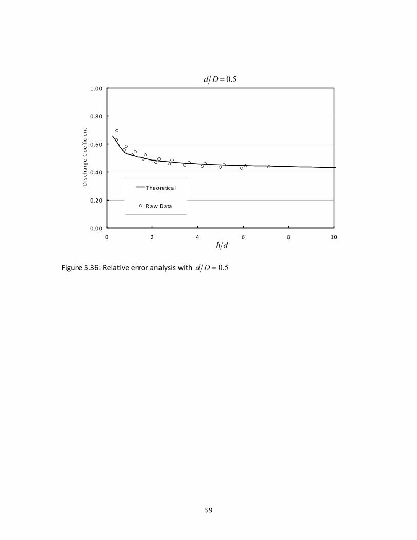
59
d/D = 0.5
0.00
0.20
0.40
0.60
0.80
1.00
0 2 4 6 8 10
Dis
ch
arg
e C
oe
ffic
ien
t
T heoretical
R aw Data
Figure 5.36: Relative error analysis with 0.5d D =
h d
0.5d D =
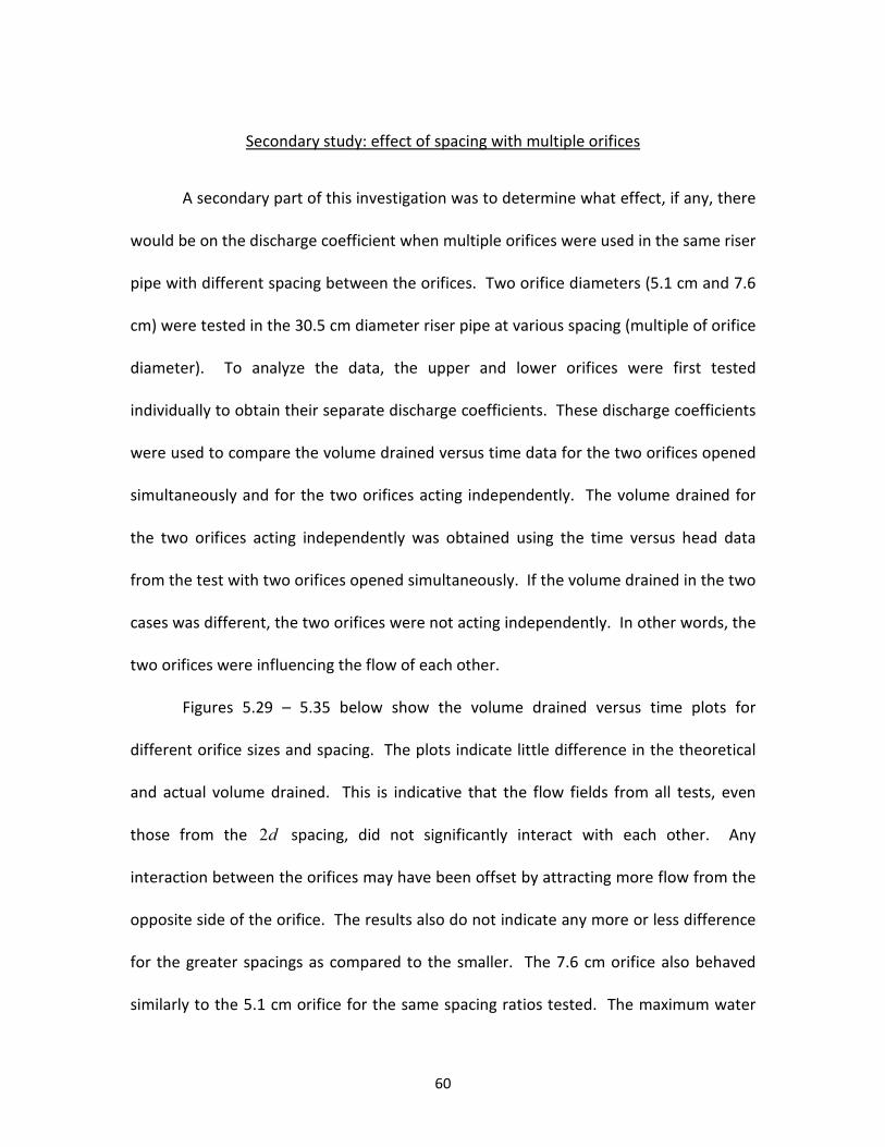
60
Secondary study: effect of spacing with multiple orifices
A secondary part of this investigation was to determine what effect, if any, there
would be on the discharge coefficient when multiple orifices were used in the same riser
pipe with different spacing between the orifices. Two orifice diameters (5.1 cm and 7.6
cm) were tested in the 30.5 cm diameter riser pipe at various spacing (multiple of orifice
diameter). To analyze the data, the upper and lower orifices were first tested
individually to obtain their separate discharge coefficients. These discharge coefficients
were used to compare the volume drained versus time data for the two orifices opened
simultaneously and for the two orifices acting independently. The volume drained for
the two orifices acting independently was obtained using the time versus head data
from the test with two orifices opened simultaneously. If the volume drained in the two
cases was different, the two orifices were not acting independently. In other words, the
two orifices were influencing the flow of each other.
Figures 5.29 – 5.35 below show the volume drained versus time plots for
different orifice sizes and spacing. The plots indicate little difference in the theoretical
and actual volume drained. This is indicative that the flow fields from all tests, even
those from the 2d spacing, did not significantly interact with each other. Any
interaction between the orifices may have been offset by attracting more flow from the
opposite side of the orifice. The results also do not indicate any more or less difference
for the greater spacings as compared to the smaller. The 7.6 cm orifice also behaved
similarly to the 5.1 cm orifice for the same spacing ratios tested. The maximum water
61
level in the tank prevented the 7.6 cm orifice from being tested at an 8d spacing. In
general the results show that orifices placed 2d or more apart could be treated as
independent orifices.
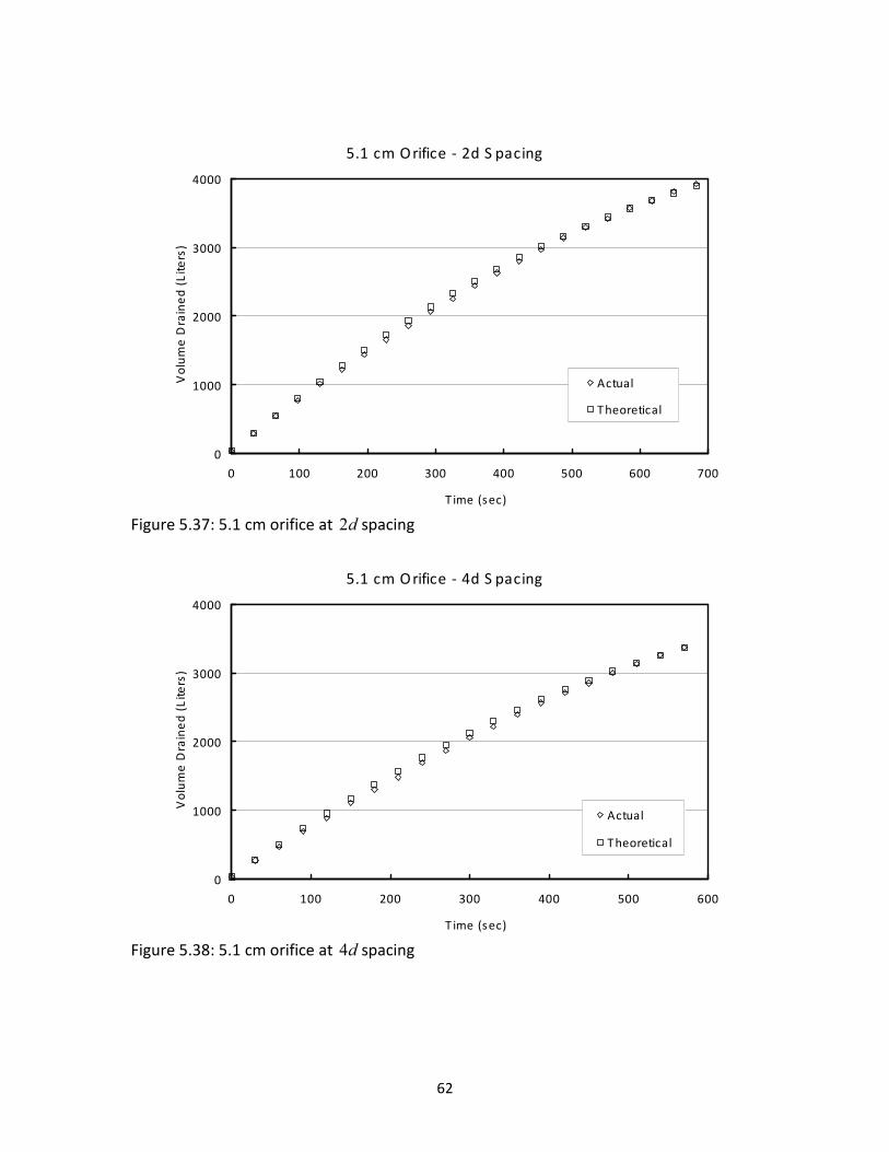
62
5.1 cm O rifice - 2d S pacing
0
1000
2000
3000
4000
0 100 200 300 400 500 600 700
T ime (sec)
Vo
lum
e D
rain
ed
(L
ite
rs)
Actual
T heoretical
Figure 5.37: 5.1 cm orifice at 2d spacing
5.1 cm O rifice - 4d S pacing
0
1000
2000
3000
4000
0 100 200 300 400 500 600
T ime (sec)
Vo
lum
e D
rain
ed
(L
ite
rs)
Actual
T heoretical
Figure 5.38: 5.1 cm orifice at 4d spacing
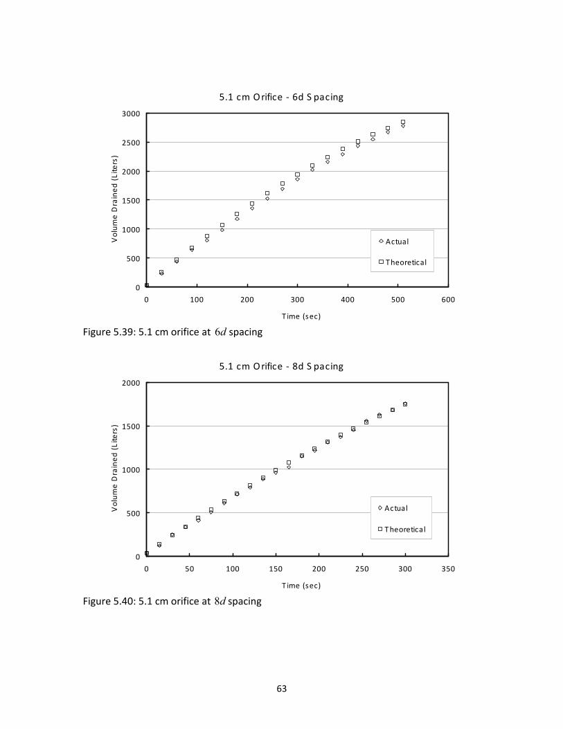
63
5.1 cm O rifice - 6d S pacing
0
500
1000
1500
2000
2500
3000
0 100 200 300 400 500 600
T ime (sec)
Vo
lum
e D
rain
ed
(L
ite
rs)
Actual
T heoretical
Figure 5.39: 5.1 cm orifice at 6d spacing
5.1 cm O rifice - 8d S pacing
0
500
1000
1500
2000
0 50 100 150 200 250 300 350
T ime (sec)
Vo
lum
e D
rain
ed
(L
ite
rs)
Actual
T heoretical
Figure 5.40: 5.1 cm orifice at 8d spacing

64
7.6 cm O rifice - 2d S pacing
0
1000
2000
3000
4000
0 50 100 150 200 250 300
T ime (s ec)
Vo
lum
e D
rain
ed
(L
ite
rs)
Actual
T heoretical
Figure 5.41: 7.6 cm orifice at 2d spacing
7.6 cm O rifice - 4d S pacing
0
500
1000
1500
2000
2500
3000
0 50 100 150 200 250
T ime (sec)
Vo
lum
e D
rain
ed
(L
ite
rs)
Actual
T heoretical
Figure 5.42: 7.6 cm orifice at 4d spacing
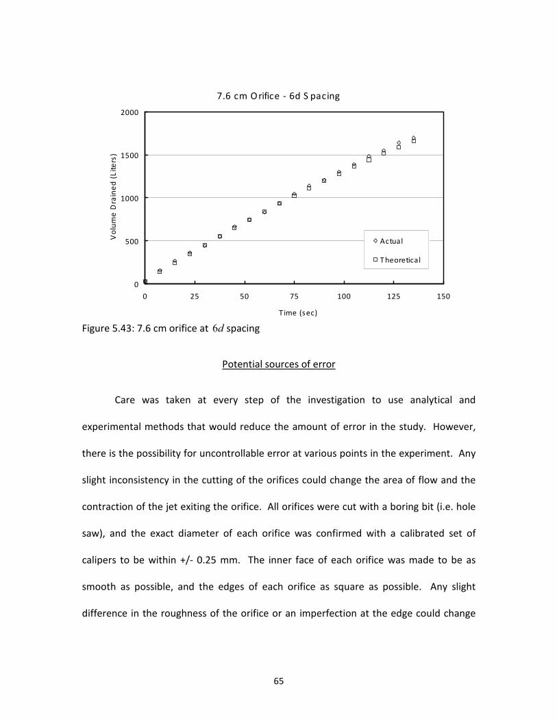
65
7.6 cm O rifice - 6d S pacing
0
500
1000
1500
2000
0 25 50 75 100 125 150
T ime (sec)
Vo
lum
e D
rain
ed
(L
ite
rs)
Actual
T heoretical
Figure 5.43: 7.6 cm orifice at 6d spacing
Potential sources of error
Care was taken at every step of the investigation to use analytical and
experimental methods that would reduce the amount of error in the study. However,
there is the possibility for uncontrollable error at various points in the experiment. Any
slight inconsistency in the cutting of the orifices could change the area of flow and the
contraction of the jet exiting the orifice. All orifices were cut with a boring bit (i.e. hole
saw), and the exact diameter of each orifice was confirmed with a calibrated set of
calipers to be within +/- 0.25 mm. The inner face of each orifice was made to be as
smooth as possible, and the edges of each orifice as square as possible. Any slight
difference in the roughness of the orifice or an imperfection at the edge could change
66
the nature of the contraction and therefore affect the discharge coefficient. The height
of the orifice above the tank floor plays a role in determining the discharge coefficient,
and any error in recording the height could affect dC . The orifice heights were
measured before testing, and the exact height of the orifice centerline was used in data
analysis.
The pressure transducer used to measure water level also could have been a
source of error for the investigation. The accuracy of the transducer as determined by
the manufacturer is 0.25% of the full scale. A constant head test showed the readings
would oscillate around the true value. However, the data for the tests was large, so any
variation would be unnoticeable. Trend line equations were used to determine the
height and volume drained, and the fit of the line may have introduced error, but all
calibration curves yielded correlation coefficients of 0.999 or greater.
Another possible source of error might be the flanges used to attach the riser
pipes to the tank floor. The flanges were approximately 8 mm thick, and the flow field
of the lowest orifice height (15.2 cm) might have been affected by the different shape of
the vertical plane. Dye tests were performed to rule out any role the flanges might have
played in the flow patterns, but it could not be determined with absolute certainty.
67
CHAPTER 6
CONCLUSIONS AND RECOMMENDATIONS
An investigation was performed to determine the discharge coefficient for
circular orifices cut into thin-walled (orifice diameter greater than pipe wall thickness)
riser pipes that might be used for an outlet control device from a stormwater detention
pond. The scenario was unique because the flow entered the riser pipe through the
orifice from outside the pipe, presenting a case of flow over a convex, or inward-curved,
surface. This study investigated a total of six different orifice sizes, ranging from 1.3 cm
(0.5 in) to 12.7 cm (5 in), at five different heights from the tank floor, ranging from 15.2
cm (6 in) to 55.9 cm (22 in). The study also utilized two different riser pipe diameters,
15.2 cm (6 in) and 30.5 cm (12 in).
The study found that for a given orifice size decreasing head values resulted in a
gradual increase in the discharge coefficient, with a more drastic increase in dC as the
water level approached the top of the orifice. This was primarily the result of a
decrease in the contraction of the jet exiting the orifice, due to the reduced velocity of
the flow approaching the orifice. For a given orifice size, the discharge coefficient
reached a constant value at high head values.
The study found that for a given orifice size as the orifice height above the tank
floor was increased, the discharge coefficient decreased, possibly the result of
suppression of the flow entering the orifice at lower heights. It was also determined
68
that at the upper-most heights (45.7 cm and 55.9 cm), dC was unaffected by the tank
floor.
The study found that increasing the d D ratio resulted in a decrease of the
discharge coefficient. This was expected as the greater the curvature effect of the
orifice, the more oblique the angles will be at which flow streamlines must enter the
orifice. This increased the transverse velocity components of the streamlines and
reduces the area of the jet at the vena contracta.
The test results from the two upper orifice heights were successfully normalized
and compiled into a single curve, which, along with a curve used to determine a
parameter oC , can be used to find the proper discharge coefficient for any orifice size in
any riser pipe diameter at any h d value.
As a secondary aim of the study, multiple orifices in the same vertical plane were
tested at several spacings based on the orifice diameter, d . The study found that the
discharge was unaffected for spacing equal or greater than 2d .
It is recommended that further investigation be undertaken to extend the results
presented here. Detailed analysis of orifice flows near a floor should be undertaken.
Also work should be undertaken on orifices of non-circular shapes with these same
parameters to determine if the discharge coefficients vary in the same fashion. Also, a
more in-depth analysis of the interaction of multiple orifices should evaluate the
changes in discharge with orifices spaced closer together than this investigation
performed, more than two orifices, and orifices in the same horizontal plane. Finally,
69
investigation should be undertaken to determine the discharge coefficient for orifices
lying in a horizontal plane, which may act similar to a weir under low heads.
70
REFERENCES
Akan, A. O. and Houghtalen, R. J. (2003). Urban Hydrology, Hydraulics, and Stormwater
Quality. John Wiley & Sons, Hoboken, N. J., pp 373.
Brater, E. F., King, H. W., Lindell, J. E., and Wei, C.Y. (1996). Handbook of Hydraulics.
McGraw-Hill, New York, N. Y.
Bryant, D. B., Khan, A. A., and Aziz, N. M. (2008). “Investigation of Flow Upstream of
Orifices.” Journal of Hydraulic Engineering, ASCE, 134(1), 98 – 104.
Gregg, W. B., Werth, D. E., and Frizzell, C. (2003). “Determination of discharge
coefficients for hydraulic sparger design.” Journal of Pressure Vessel Technology,
ASME, 126(3), 354 – 359.
Gupta, R. S. (2008). Hydrology and Hydraulic Systems. Waveland Press, Long Grove,
Illinois., pp 896.
Jarrett, A. R. (1993). “Design of Perforated Risers to Control Dewatering of
Sedimentation Basins.” Applied Engineering in Agriculture, ASAE, 9(1), 37 – 42.
Millen, J. A., Jarrett, A. R., and Faircloth, J. W. (1997). “Experimental Evaluation of
Sedimentation Basin Performance for Alternative Dewatering Systems.”
Transactions of the ASAE, ASAE, 40(4), 1087 – 1095.
Smith, D., and Walker, W. J. (1923). “Orifice Flow.” Institution of Mechanical Engineers –
Proceedings, 1, 23 – 36.
Smith, Hamilton, Jr. (1886). Hydraulics. John Wiley & Sons, New York, N. Y., pp 421.
Tsihrintzis, V. A., and Hamid, R. (1997). “Modeling and Management of Urban
Stormwater Runoff Quality: A Review.” Water Resources Management, 11(2), 137 –
164.
71
Werth, D. E., Khan, A. A., and Gregg, W. B. (2005). “Experimental study of wall curvature
and bypass flow effects on orifice discharge coefficients.” Experiments in Fluids, 39,
485 – 491.