1

Progress in NASA Heliogyro Solar Sail Structural Dynamics

and Solarelastic Stability Research

Jer-Nan JUANG1), Jerry E. WARREN2), Lucas G. HORTA2) and W. Keats WILKIE2)

1)National Institute of Aerospace, Hampton, Virginia, USA

2)Structural Dynamics Branch, NASA Langley Research Center, Hampton, Virginia, USA

Recent NASA-sponsored research on the structural dynamics of the heliogyro has produced significant advances in heliogyro solarelasticity modeling capabilities, small-scale structural dynamics ground verification testing methods, and system identification procedures for on-orbit heliogyro blade dynamics investigations. These earlier studies were based on the simplifying assumption of a fixed rotational rate for a single heliogyro sail blade. In this paper, we will develop an analytical dynamic model for a freely-spinning heliogyro discretized by continuous beam mode shapes. Numerical results using the dynamic model with multiple blades coupled to a rotationally unconstrained central spacecraft bus hub will be presented. This nonlinear model will include dynamic coupling of rigid body motion of the central hub, radiation pressure forces, and the vibrational motion of the blades. Solarelastic stability results will be compared with analysis of simulated time domain data generated using a fully-coupled, nonlinear finite element model of the multi-bladed heliogyro. Parameter sensitivity of the solarelastic stability behavior is examined and also presented by using global sensitivity metrics in terms of variance.

Key Words: Solar sail, Solarelastic stability, Heliogyro dynamics

Nomenclature c : blade width E : Young’s modulus

ebx ,ebη ,ebζ : orthogonal unit vector of blade frame

eIx ,eIy ,eIz

: orthogonal unit vector of inertia frame

ehx ,ehy ,ehz

eIx ,eIy ,eIz

: orthogonal unit vector of hub frame G : torsional rigidity; G ≈ E / [2(1+υ)]

ℓ : blade length mb : blade density per unit length; kg/m2 p0 : solar radiation pressure

p : nondimensional p0 ;p = p0c( ) mbΩ02( )

Rx , Ry , Rz

: translation of the hub frame

Rx , Ry , Rz

: Rx = Rx ℓ , Ry = Ry ℓ , Rz = Rz ℓ

u,v,w,φ

: elastic displacements, and twist angle

u ,v ,w

: u = u ℓ , v = v ℓ , w = w ℓ

v ',w '

: v ' = ∂v ∂x ,w ' = ∂w ∂x

x, y,z

: hub coordinate

θx ,θ y ,θ z

: rotational angles of the hub frame

Ω0

: nominal spin rate of heliogyro, rad/sec

ϕui ,ϕui ,ϕwi ,ϕφi

: ith mode shape for elastic displacements υ

: poison ratio

Subscripts i , j, k : integers for indexing mode shapes

1. Introduction Recent studies on the heliogyro have produced significant advances in heliogyro solarelasticity modeling capabilities, small-scale structural dynamics ground verification testing methods, and system identification procedures for on-orbit

heliogyro blade dynamics investigations.1-5) A significant finding of these earlier studies was that mathematical models of freely-spinning heliogyro systems, i.e., ones where the simplifying assumption of a fixed rotational rate has been removed, may not exhibit certain solarelastic instabilities shown for single blade heliogyro models6-7) with the spin rate remaining constant. In this paper, we will develop a free-spinning multi-bladed dynamic model discretized by continuous beam mode shapes. This nonlinear model will include dynamic coupling of rigid body motion of the central hub, radiation pressure forces, and the vibrational motion of the blades. A complete derivation of the new mathematical heliogyro blade model will be presented, along with a description of the coupled nonlinear finite element model and methodology used to simulate the time domain behavior of the heliogyro. Numerical results from a new study using the heliogyro mathematical model with multiple blades coupled to a rotationally unconstrained central hub will be shown and discussed. Solarelastic stability results using the analytical heliogyro dynamics model will be compared with analysis of simulated time domain data generated using the fully coupled, nonlinear finite element model of the multi-bladed heliogyro. Solarelastic stability behavior of both single and multi-bladed heliogyro solar sails will be examined. Examples of stability results using the newer analytical model will be shown for a reference heliogyro blade concept. Parameter sensitivity using global sensitivity metrics in terms of variance, i.e., the total variance of a particular root when all parameters are varied, will be compared with the per-parameter variance and also presented. 2. Free Spinning Equations of Motion Three coordinate frames are used to derive the heliogyro

structural dynamic equations of motion. The first is a blade coordinate frame to describe blade deformation. The second is the hub frame, which is used to express the hub rotational motion. The third is the inertia frame, used for the translational motion of the origin of the hub frame.

2

Ω0

x, ehx

y, ehy

z, ehz

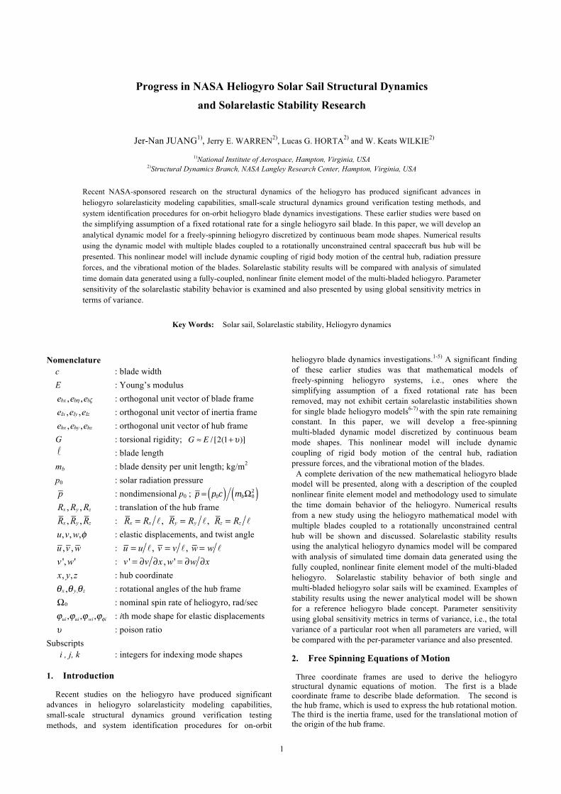
Fig. 1. Two blades attached to a rigid hub, with hub frame indicated.

An arbitrary position on a blade after deformation can be written by

!rb = RxeIx + RyeIy + RIzeIz + Hhxehx+ x + u − v ' η cosφ −ζ sinφ( )−w ' η sinφ +ζ cosφ( )⎡⎣ ⎤⎦ehx+ v +η cosφ −ζ sinφ[ ]ehy + w +η sinφ +ζ cosφ[ ]ehy

(1)

The variable Hhx is the distance from the center of the hub frame to the root of the blade. The variable x is the distance from the root of the blade and u is the elongation displacement of the blade along ehx, v is the in-plane displacement along the ehy axis and w is the out-of-plane displacement along ehz. Note that the position vector is derived using beam theory and all higher-order terms are ignored.8-10) Based on the position vector shown in Eq. (1), it is possible to derive the stress tensor for computing potential energy V, and kinetic energy T by taking the derivative of Eq. (1) with respect to time t. The angular velocity of the blade expressed in terms of the hub frame is

!ω = "θ x −

"θ z +Ω0( )sinθ y⎡⎣⎢

⎤⎦⎥ehx

+ "θ y cosθ x +"θ z +Ω0( )cosθ y sinθ x

⎡⎣⎢

⎤⎦⎥ehy

+ − "θ y sinθ x +"θ z +Ω0( )cosθ y cosθ x

⎡⎣⎢

⎤⎦⎥ehz

(2)

Knowing T and V of the blade, application of Hamilton’s principle yields variation quantities of T-V in terms of

δ Rx ,δ Ry ,δ Rz for translation, δθ x ,δθ y ,δθ z for rotation, and

δu,δv,δw,δφ for blade deflection, that, in turn, produces the equations of motion. There are three coordinate frames involved in Eq. (1). It is convenient to transform them to the hub frame with a nominal spinning rate Ω0 about the ehz axis. Reducing the equations of motion to include the linear and second-order nonlinear terms yields the matrix equation as follows.

M!!q +C !q + Kq = fq (3)

where q is the generalized coordinate vector

q = Rx Ry Rz θ x θ y θ z qwi qvi qφi qui

⎡⎣

⎤⎦

T

; i = 1,2,…n (4)

and fq is the generalized force vector, with the assumption that all deflection quantities are function separable, i.e

u x,t( ) = qui t( )ϕui x( ); v x,t( ) = qvi t( )ϕvi x( ); w x,t( ) = qwi t( )ϕwi x( ); φ x,t( ) = qφi t( )ϕφi x( ) (5)

Note that double subscript integer index i implies summation

from i = 1,2,…,n where n is the number of shape functions used to approximate its associated continuous quantity. The mass matrix M , the gyroscopic matrix C , and the nonlinear stiffness matrix K for a spinning blade are explicitly shown in the appendix. The over bar on a quantity indicates that it is a non-dimensional quantity according to the rules also shown in the appendix. The generalized force vector consists of internal centrifugal force and external forces such as solar radiation force. Consider the simple case where the vector of sun illumination is aligned with the spinning axis. The resulting generalized forces are9-10)

fRx = pθ y − pqwj ϕwj'

0

1

∫ dξ; fRy = − pθ x − pqφ j ϕφ j0

1

∫ dξ; fRz = p

fθx = pqvj ϕvj0

1

∫ dξ; fθ y = − p ξ0

1

∫ dξ;

fθz = − pθ x ξ0

1

∫ dξ − pqφ j ξϕφ j0

1

∫ dξ;

fqwi= p ϕwi0

1

∫ dξ; fqvi= − pqφ j ϕviϕφ j0

1

∫ dξ;

(6)

Note that coordinate-dependent terms fRx , fRy , fθx , fθz , fqvi can be inserted into the stiffness matrix (see Appendix). The term

fqvi yields one-way coupling from twisting to in-plane motion. The generalized constant force vector thus becomes

fq = 0 0 p 0 fθy 0 fqwi 0 0 −Tx'ϕui −ξϕui

⎡⎣⎢

⎤⎦⎥

T

(7)

where the last term inside the vector comes from the potential and kinetic energies associated with the variation of the elongation u. Assuming that the elongation u is negligible [i.e., setting qui = 0 in Eq.(3)], the non-dimensional tension force Tx caused by the centrifugal force due to the spinning rate Ω0 is calculated by

Tx = − !!Rx − !Ry − 2ξ!θ z − 2ϕv

!qvi −ξ( )ξ

1

∫ dξ

= − 1−ξ( ) !!Rx + 1−ξ( ) !Ry + 1−ξ2( ) !θ z

+2 ϕvi dξξ

1

∫( ) !qvi + 12 1−ξ 2( ) (8)

Equations (1)-(8) complete the process of deriving dynamic equations for a single blade. The approach can be easily extended for any additional blades attached to the hub. One may simply transform the orientation of the position vector shown in Eq. (1) to a new blade coordinate frame to derive its own set of matrix equations as shown in Eq. (3). The overall system dynamic equations can then be obtained by interconnecting the matrix equations together for all blades. For example, the equations of motion for two blades attached to a hub shown in Fig. 1 will have three translational coordinates, three rotational coordinates, and 6n generalized coordinates to describe the two-blade deflections including in-plane and out-of-plane deflections, and twisting angles. 3. Stability and Sensitivity Analyses For cases where a constant solar radiation pressure is applied to

the blades, for example, when the spin axis of the heliogyro is oriented toward the sun, a static deflection will occur. When the solar illumination is aligned with the spinning axis, the blade static deflection can be solved linearly by

qw0i = EIwϕwi

′′ ϕwj′′ +Txϕwi

' ϕwj' − km1

2 ϕwi' ϕwj

' dξ0

1

∫⎡⎣⎢⎤⎦⎥−1

fqwi ; i = 1,…,n (9)

This solution satisfies the nonlinear static equation with qv0i = qφ0i = 0 for the case of one blade. It is also valid for the case of two “identical” blades attached to the hub as shown in

3

Fig.1. Inserting the static solution, Eq. (9), into the system equations yields a linear matrix equation that allows us to solve for system eigenvalues to conduct stability and sensitivity analyses.

3.1. Flutter instability of the two-blade Heliogyro

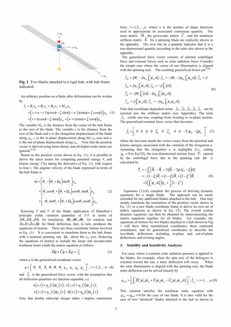
Nominal parameters for the two-blade model shown in Fig. 1 are given in Table 1. For simplicity in studying the solarelastic stability problem, we restrain the translational motions to eliminate translational divergence. We also have added 5×10-4 to the non-dimensional stiffness element associated with the hub x-axis to avoid rotational divergence for very small values of solar radiation pressure. Note that the non-dimensional stiffness for the y-axis is 0.67 obtained from the nominal parameters of the blade. Additional blades attached to the hub will avoid such a divergence problem. Fig. 2 shows modal frequency for both the fixed rotational

speed (i.e., hub-driven) heliogyro blade, and the free-spinning two-bladed heliogyro as a function of solar radiation pressure. Nominal rotational speed for both cases is 0.6 RPM. Note that 20 beam mode shapes are used. Both cases are substantially similar, although the two-bladed, free-spinning configuration now includes distinct “antisymmetric” coupled blade modes. These coupled modes disappear as hub rotational inertias tend to infinity, essentially reproducing the dynamics of the fixed rotational speed, single blade case. Both configurations indicate a blade flutter instability, i.e., an instability where the first in-plane and first twisting vibrational modes have coalesced into a complex mode with positive damping, near a radiation pressure of 7.2 ×10-6 N/m2. Instabilities at higher solar radiation pressure are also observed, most notably, the divergence instabilities occurring between 11 to 12×10-6 N/m2.

p0 : solar radiation pressure

ωΩ0

×10−6 N m26 8 10 12 14

1

2

3

4

a)

p0 : solar radiation pressure

ωΩ0

×10−6 N m26 8 10 12 14

1

2

3

4

b)

Fig. 2 Normalized modal frequencies of a) the fixed rotational speed heliogyro blade, and b) the free-spinning two-bladed heliogyro as a function of solar radiation pressure. Ω0 = 0.6 RPM

Table 1 Nominal Blade Parameters and Ranges for Sensitivity Studies

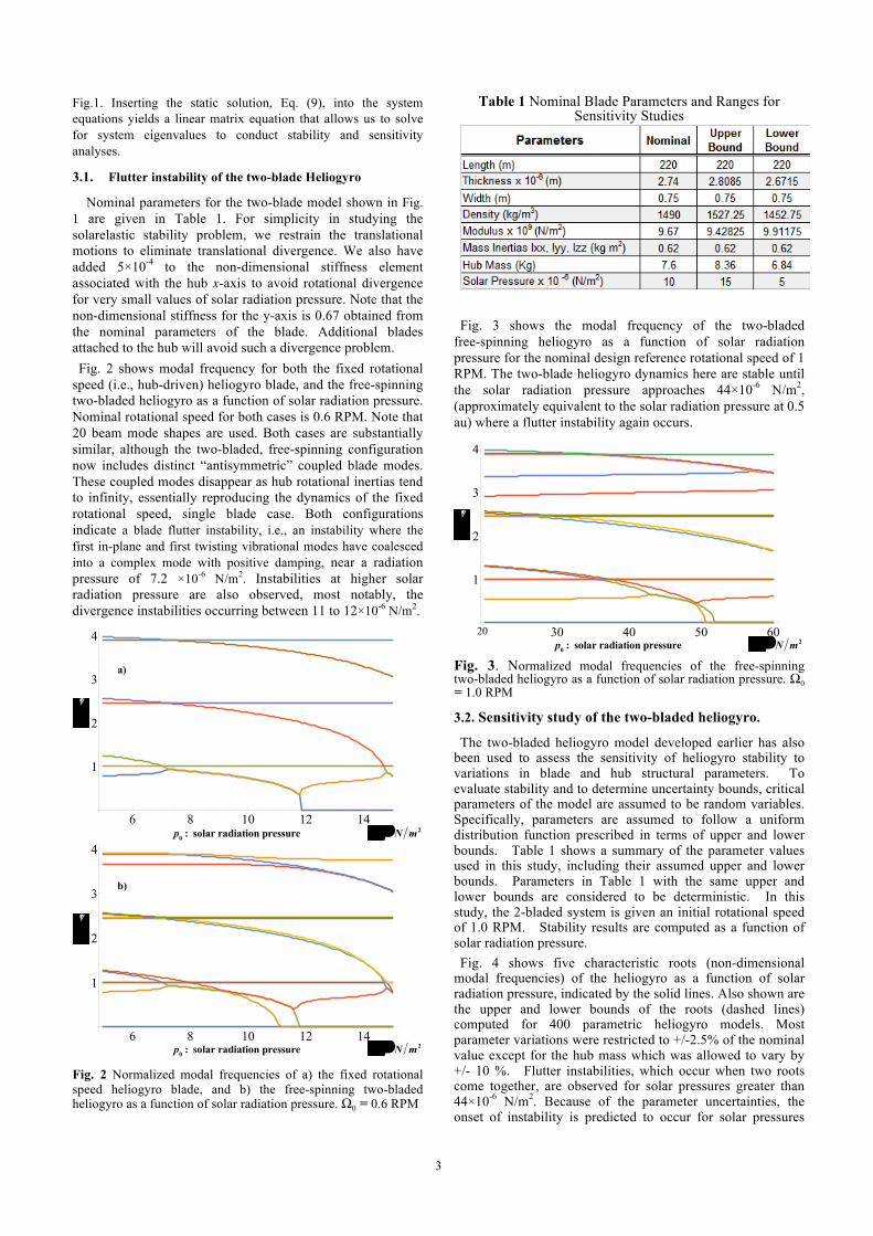
Fig. 3 shows the modal frequency of the two-bladed

free-spinning heliogyro as a function of solar radiation pressure for the nominal design reference rotational speed of 1 RPM. The two-blade heliogyro dynamics here are stable until the solar radiation pressure approaches 44×10-6 N/m2, (approximately equivalent to the solar radiation pressure at 0.5 au) where a flutter instability again occurs.

p0 : solar radiation pressure

ωΩ0

×10−6 N m230 40 50 60

1

2

3

4

20

Fig. 3. Normalized modal frequencies of the free-spinning two-bladed heliogyro as a function of solar radiation pressure. Ω0 = 1.0 RPM

3.2. Sensitivity study of the two-bladed heliogyro.

The two-bladed heliogyro model developed earlier has also been used to assess the sensitivity of heliogyro stability to variations in blade and hub structural parameters. To evaluate stability and to determine uncertainty bounds, critical parameters of the model are assumed to be random variables. Specifically, parameters are assumed to follow a uniform distribution function prescribed in terms of upper and lower bounds. Table 1 shows a summary of the parameter values used in this study, including their assumed upper and lower bounds. Parameters in Table 1 with the same upper and lower bounds are considered to be deterministic. In this study, the 2-bladed system is given an initial rotational speed of 1.0 RPM. Stability results are computed as a function of solar radiation pressure. Fig. 4 shows five characteristic roots (non-dimensional

modal frequencies) of the heliogyro as a function of solar radiation pressure, indicated by the solid lines. Also shown are the upper and lower bounds of the roots (dashed lines) computed for 400 parametric heliogyro models. Most parameter variations were restricted to +/-2.5% of the nominal value except for the hub mass which was allowed to vary by +/- 10 %. Flutter instabilities, which occur when two roots come together, are observed for solar pressures greater than 44×10-6 N/m2. Because of the parameter uncertainties, the onset of instability is predicted to occur for solar pressures

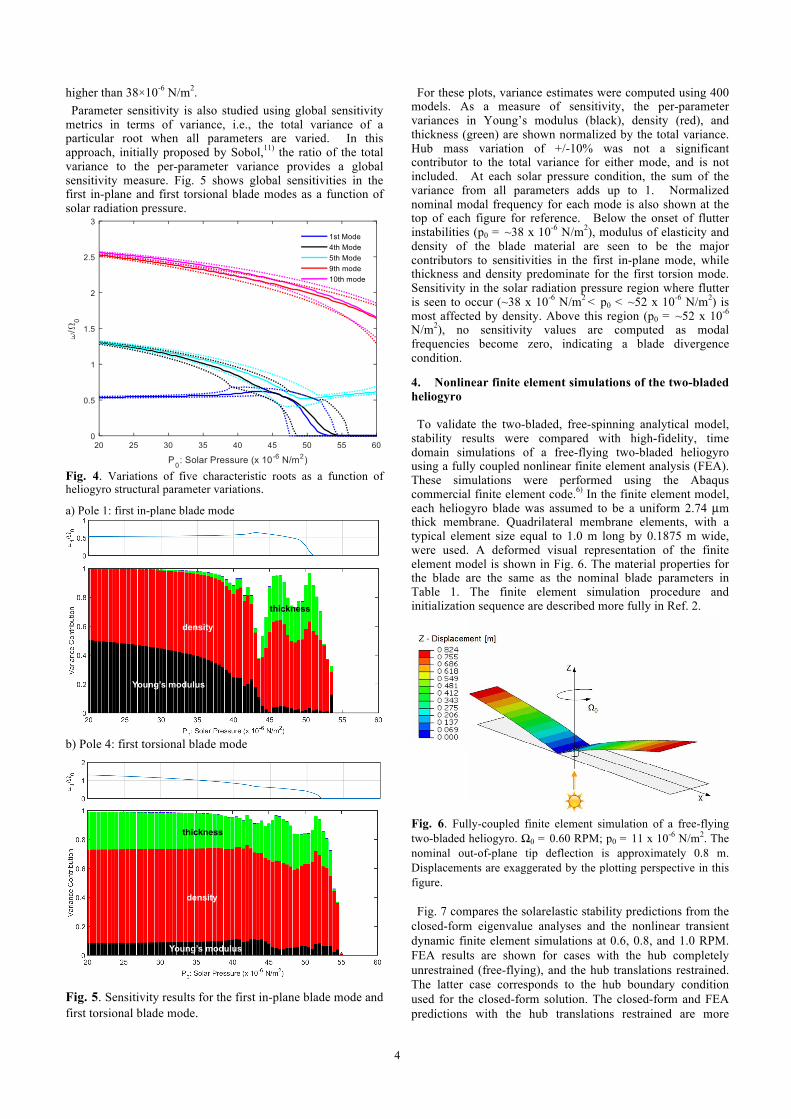
4

higher than 38×10-6 N/m2. Parameter sensitivity is also studied using global sensitivity

metrics in terms of variance, i.e., the total variance of a particular root when all parameters are varied. In this approach, initially proposed by Sobol,11) the ratio of the total variance to the per-parameter variance provides a global sensitivity measure. Fig. 5 shows global sensitivities in the first in-plane and first torsional blade modes as a function of solar radiation pressure.

Fig. 4. Variations of five characteristic roots as a function of heliogyro structural parameter variations.

a) Pole 1: first in-plane blade mode

thickness

density

Young’s modulus

b) Pole 4: first torsional blade mode

thickness

density

Young’s modulus

Fig. 5. Sensitivity results for the first in-plane blade mode and first torsional blade mode.

For these plots, variance estimates were computed using 400 models. As a measure of sensitivity, the per-parameter variances in Young’s modulus (black), density (red), and thickness (green) are shown normalized by the total variance. Hub mass variation of +/-10% was not a significant contributor to the total variance for either mode, and is not included. At each solar pressure condition, the sum of the variance from all parameters adds up to 1. Normalized nominal modal frequency for each mode is also shown at the top of each figure for reference. Below the onset of flutter instabilities (p0 = ~38 x 10-6 N/m2), modulus of elasticity and density of the blade material are seen to be the major contributors to sensitivities in the first in-plane mode, while thickness and density predominate for the first torsion mode. Sensitivity in the solar radiation pressure region where flutter is seen to occur (~38 x 10-6 N/m2 < p0 < ~52 x 10-6 N/m2) is most affected by density. Above this region (p0 = ~52 x 10-6 N/m2), no sensitivity values are computed as modal frequencies become zero, indicating a blade divergence condition. 4. Nonlinear finite element simulations of the two-bladed heliogyro To validate the two-bladed, free-spinning analytical model,

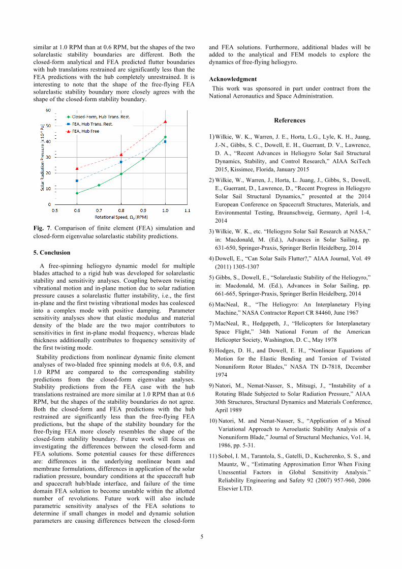
stability results were compared with high-fidelity, time domain simulations of a free-flying two-bladed heliogyro using a fully coupled nonlinear finite element analysis (FEA). These simulations were performed using the Abaqus commercial finite element code.6) In the finite element model, each heliogyro blade was assumed to be a uniform 2.74 µm thick membrane. Quadrilateral membrane elements, with a typical element size equal to 1.0 m long by 0.1875 m wide, were used. A deformed visual representation of the finite element model is shown in Fig. 6. The material properties for the blade are the same as the nominal blade parameters in Table 1. The finite element simulation procedure and initialization sequence are described more fully in Ref. 2.

Fig. 6. Fully-coupled finite element simulation of a free-flying two-bladed heliogyro. Ω0 = 0.60 RPM; p0 = 11 x 10-6 N/m2. The nominal out-of-plane tip deflection is approximately 0.8 m. Displacements are exaggerated by the plotting perspective in this figure. Fig. 7 compares the solarelastic stability predictions from the

closed-form eigenvalue analyses and the nonlinear transient dynamic finite element simulations at 0.6, 0.8, and 1.0 RPM. FEA results are shown for cases with the hub completely unrestrained (free-flying), and the hub translations restrained. The latter case corresponds to the hub boundary condition used for the closed-form solution. The closed-form and FEA predictions with the hub translations restrained are more

5

similar at 1.0 RPM than at 0.6 RPM, but the shapes of the two solarelastic stability boundaries are different. Both the closed-form analytical and FEA predicted flutter boundaries with hub translations restrained are significantly less than the FEA predictions with the hub completely unrestrained. It is interesting to note that the shape of the free-flying FEA solarelastic stability boundary more closely agrees with the shape of the closed-form stability boundary.

Fig. 7. Comparison of finite element (FEA) simulation and closed-form eigenvalue solarelastic stability predictions. 5. Conclusion A free-spinning heliogyro dynamic model for multiple blades attached to a rigid hub was developed for solarelastic stability and sensitivity analyses. Coupling between twisting vibrational motion and in-plane motion due to solar radiation pressure causes a solarelastic flutter instability, i.e., the first in-plane and the first twisting vibrational modes has coalesced into a complex mode with positive damping. Parameter sensitivity analyses show that elastic modulus and material density of the blade are the two major contributors to sensitivities in first in-plane modal frequency, whereas blade thickness additionally contributes to frequency sensitivity of the first twisting mode. Stability predictions from nonlinear dynamic finite element

analyses of two-bladed free spinning models at 0.6, 0.8, and 1.0 RPM are compared to the corresponding stability predictions from the closed-form eigenvalue analyses. Stability predictions from the FEA case with the hub translations restrained are more similar at 1.0 RPM than at 0.6 RPM, but the shapes of the stability boundaries do not agree. Both the closed-form and FEA predictions with the hub restrained are significantly less than the free-flying FEA predictions, but the shape of the stability boundary for the free-flying FEA more closely resembles the shape of the closed-form stability boundary. Future work will focus on investigating the differences between the closed-form and FEA solutions. Some potential causes for these differences are: differences in the underlying nonlinear beam and membrane formulations, differences in application of the solar radiation pressure, boundary conditions at the spacecraft hub and spacecraft hub/blade interface, and failure of the time domain FEA solution to become unstable within the allotted number of revolutions. Future work will also include parametric sensitivity analyses of the FEA solutions to determine if small changes in model and dynamic solution parameters are causing differences between the closed-form

and FEA solutions. Furthermore, additional blades will be added to the analytical and FEM models to explore the dynamics of free-flying heliogyro.

Acknowledgment This work was sponsored in part under contract from the

National Aeronautics and Space Administration.

References

1) Wilkie, W. K., Warren, J. E., Horta, L.G., Lyle, K. H., Juang, J.-N., Gibbs, S. C., Dowell, E. H., Guerrant, D. V., Lawrence, D. A., “Recent Advances in Heliogyro Solar Sail Structural Dynamics, Stability, and Control Research,” AIAA SciTech 2015, Kissimee, Florida, January 2015

2) Wilkie, W., Warren, J., Horta, L. Juang, J., Gibbs, S., Dowell, E., Guerrant, D., Lawrence, D., “Recent Progress in Heliogyro Solar Sail Structural Dynamics,” presented at the 2014 European Conference on Spacecraft Structures, Materials, and Environmental Testing, Braunschweig, Germany, April 1-4, 2014

3) Wilkie, W. K., etc. “Heliogyro Solar Sail Research at NASA,” in: Macdonald, M. (Ed.), Advances in Solar Sailing, pp. 631-650, Springer-Praxis, Springer Berlin Heidelberg, 2014

4)Dowell, E., “Can Solar Sails Flutter?,” AIAA Journal, Vol. 49 (2011) 1305-1307

5) Gibbs, S., Dowell, E., “Solarelastic Stability of the Heliogyro,” in: Macdonald, M. (Ed.), Advances in Solar Sailing, pp. 661-665, Springer-Praxis, Springer Berlin Heidelberg, 2014

6) MacNeal, R., “The Heliogyro: An Interplanetary Flying Machine,” NASA Contractor Report CR 84460, June 1967

7) MacNeal, R., Hedgepeth, J., “Helicopters for Interplanetary Space Flight,” 34th National Forum of the American Helicopter Society, Washington, D. C., May 1978

8) Hodges, D. H., and Dowell, E. H., “Nonlinear Equations of Motion for the Elastic Bending and Torsion of Twisted Nonuniform Rotor Blades,” NASA TN D-7818, December 1974

9) Natori, M., Nemat-Nasser, S., Mitsugi, J., “Instability of a Rotating Blade Subjected to Solar Radiation Pressure,” AIAA 30th Structures, Structural Dynamics and Materials Conference, April 1989

10) Natori, M. and Nenat-Nasser, S., “Application of a Mixed Variational Approach to Aeroelastic Stability Analysis of a Nonuniform Blade,” Journal of Structural Mechanics, Vo1. l4, 1986, pp. 5-31.

11) Sobol, I. M., Tarantola, S., Gatelli, D., Kucherenko, S. S., and Mauntz, W., “Estimating Approximation Error When Fixing Unessential Factors in Global Sensitivity Analysis.” Reliability Engineering and Safety 92 (2007) 957-960, 2006 Elsevier LTD.

6

Appendix Definitions of sectional integrals are given as follows

ρ dηdζA∫∫ = m = ρA (for constant ρ and A)

ρηdηdζA∫∫ = 0; ρζ dηdζ

A∫∫ = 0

ρη2 dηdζA∫∫ = mkm2

2 ; ρζ 2 dηdζA∫∫ = mkm1

2 ;

ρ η −ζ[ ] η +ζ[ ]dηdζA∫∫ = m km2

2 − km12( ) = mΔkm2

ρ η2 +ζ 2( )dηdζA∫∫ = m km2

2 + km12( ) = mkm2

Iv = η2 dηdζA∫∫ ; Iw == ζ 2 dηdζ

A∫∫ ; Aka2 = η2 +ζ 2( )dηdζ

A∫∫A = dηdζ

A∫∫ ; ζ dηdζ = 0A∫∫ ; ηζ dηdζ

A∫∫ = 0; J ≈ 4 Iw

Non-dimensional parameters are calculated by

ξ= xℓ

; "θ x ="θ x

Ω0

; ""θ x =""θ x

Ω02 ; "θ y =

"θ y

Ω0

; "θ y =""θ y

Ω02 ; "θ z =

"θ z

Ω0

; ""θ z =""θ z

Ω02

T = TmΩ0

2ℓ2 ; GJ = GJmΩ0

2ℓ4 ; EIw =EIw

mΩ02ℓ4 ;

EIv =EI2

mΩ02ℓ4 ; ΔEI = EIv − EIw

u = uℓ

, v = vℓ

, w = wℓ

:

t = Ω0t⇒∂( )∂t

=Ω0 ∂( )∂t

; ∂φ∂ξ

= ∂φ∂ x ℓ( ) =

ℓ∂φ∂x

v ' = ∂v∂ξ

=∂ v ℓ( )∂ x ℓ( ) = v '; v "=

∂2 v ℓ( )∂ x2 ℓ2( ) = Rv";

""v ' = d 2

Ω02dt 2

∂ v ℓ( )∂ x ℓ( ) =

1Ω0

2 ""v '

Tx' = ∂Tx

∂ξ= ∂Tx∂ x ℓ( ) =

1mΩ0

2ℓ∂Tx∂x

;

dvdt

=d v ℓ( )dΩ0t

= 1ℓΩ0

dvdt

⇒ Ω0 "vℓ2Ω0

2 = ℓΩ02 "v

ℓ2Ω02 ⇒

"vℓ

km = kmℓ

, km1=km1

ℓ, km2

=km2

ℓ

The stiffness matrix KP with non-linear off-diagonal submatrices is derived from the blade strain energy. KP = K dξ

0

1

∫ ; ΔEI = EIv − EIw;

K =

EIwϕwi′′ ϕwj

′′ +Txϕwi' ϕwj

' qφk

ΔEIϕφkϕvj′′ϕwi

′′

−EIvϕvj′′ϕwi

′ ϕφ j′

+EIwϕvj′ ϕwi

′′ ϕφ j′

⎡

⎣

⎢⎢⎢

⎤

⎦

⎥⎥⎥qvk

ΔEIϕφ jϕvk′′ ϕwi

′′

−EIvϕvk′′ ϕwi

′ ϕφ j′

+EIwϕvk′ ϕwi

′′ ϕφ j′

⎡

⎣

⎢⎢⎢

⎤

⎦

⎥⎥⎥

qφk

ΔEIϕφkϕvi′′ϕwj

′′

−EIvϕvi′′ϕwj

′ ϕφk′

+EIwϕvi′ ϕwj

′′ ϕφk′

⎡

⎣

⎢⎢⎢

⎤

⎦

⎥⎥⎥EIvϕvi

′′ϕvj′′ +Txϕvi

′ ϕvj′ qwk

ΔEIϕφ jϕvi′′ϕwk

′′

−EIvϕvi′′ϕwk

′ ϕφ j′

+EIwϕvi′ ϕwk

′′ ϕφ j′

⎡

⎣

⎢⎢⎢

⎤

⎦

⎥⎥⎥

qvk

ΔEIϕφiϕkj′′ϕwj

′′

−EIvϕvk′′ ϕwj

′ ϕφi′

+EIwϕvk′ ϕwj

′′ ϕφi′

⎡

⎣

⎢⎢⎢

⎤

⎦

⎥⎥⎥qwk

ΔEIϕφiϕvj′′ϕwk

′′

−EIvϕvj′′ϕwk

′ ϕφi′

+EIwϕvj′ ϕwk

′′ ϕφi′

⎡

⎣

⎢⎢⎢

⎤

⎦

⎥⎥⎥

GJϕφi′ ϕφ j

′

+ka2Txϕφi′ ϕφ j

′

⎡

⎣

⎢⎢⎢⎢⎢⎢⎢⎢⎢⎢⎢⎢⎢⎢

⎤

⎦

⎥⎥⎥⎥⎥⎥⎥⎥⎥⎥⎥⎥⎥⎥

The mass matrix M , the gyroscopic matrix C , and the stiffness matrix K are derived from the blade kinetic energy.

M = M dξ;0

1

∫ M =

1 0 0 0 0 0 0 0 0 ϕuj0 1 0 0 0 ξ 0 ϕvj 0 00 0 1 0 −ξ 0 ϕwj 0 0 00 0 0 km

2 0 0 0 0 km2ϕφ j 0

0 0 −ξ 0 km12 + ξ 2( ) 0 −

ϕwj' km1

2

+ξϕwj

⎛

⎝⎜

⎞

⎠⎟ 0 0 0

0 ξ 0 0 0 km22 + ξ 2 0

ϕvj' km2

2

+ξϕvj

⎛

⎝⎜

⎞

⎠⎟ 0 0

0 0ϕw 0 −ϕwj

' km12

+ξϕwj

⎛

⎝⎜

⎞

⎠⎟ 0

ϕwiϕwj +

km12ϕwi

' ϕwj'

⎛

⎝⎜

⎞

⎠⎟ 0 0 0

0ϕv 0 0 0ϕvj

' km22

+ξϕvj

⎛

⎝⎜

⎞

⎠⎟ 0

ϕviϕvj +

km22 ϕvi

' ϕvj'

⎛

⎝⎜

⎞

⎠⎟ 0 0

0 0 0 km2ϕφ j 0 0 0 0 km

2ϕφiϕφ j 0ϕui 0 0 0 0 0 0 0 0 ϕuiϕuj

⎛

⎝

⎜⎜⎜⎜⎜⎜⎜⎜⎜⎜⎜⎜⎜⎜⎜⎜⎜⎜⎜⎜

⎞

⎠

⎟⎟⎟⎟⎟⎟⎟⎟⎟⎟⎟⎟⎟⎟⎟⎟⎟⎟⎟⎟

C = C dξ0

1

∫ ; C =

0 0 0 0 0 −ξ 0 −ϕvj 0 00 0 0 0 0 0 0 0 0 ϕuj

0 0 0 0 0 0 0 0 0 00 0 0 0 −2km1

2 0 2km12 ϕwj

' 0 0 00 0 0 2km1

2 0 0 0 0 2km12 ϕφ j 0

ξ 0 0 0 0 0 0 0 0 2ϕujξ0 0 0−2km1

2 ϕwi' 0 0 0 0 −2km1

2 ϕφ jϕwi' 0

ϕv 0 0 0 0 0 0 0 0 2ϕujϕvi

0 0 0 0 −2km12 ϕφ 0 2km1

2 ϕφϕw′ 0 0 00 −ϕui 0 0 0 −2ϕuiξ 0 −2ϕuiϕvj 0 0

⎛

⎝

⎜⎜⎜⎜⎜⎜⎜⎜⎜⎜⎜⎜⎜

⎞

⎠

⎟⎟⎟⎟⎟⎟⎟⎟⎟⎟⎟⎟⎟

KT =⌢KT dξ;

0

1

∫ Δkm2 = km2

2 − km12 ; ⌢KT =

0 − p 0 0 0 0 pϕwj' 0 0 0

p 0 0 0 0 0 0 0 pϕφ j 00 0 0 0 0 0 0 0 0 00 0 0 Δkm

2 0 0 0 − pϕvj ϕφ jΔkm2 0

0 0 0 0 ξ 2 − km12 0

−ξϕwj +km1

2 ϕwj'

⎛⎝⎜

⎞⎠⎟

0 0 0

pξ 0 0 0 0 0 0 0 pξϕφ j 0

0 0 0 0−ξϕwi +km1

2 ϕwi'

⎛⎝⎜

⎞⎠⎟

0 −km12 ϕwi

' ϕwj' 0 0 0

0 0 0 0 0 0 0−ϕviϕvj −km2

2 ϕvi' ϕvj

'⎛⎝⎜

⎞⎠⎟

pϕviϕφ j 0

0 0 0 ϕφiΔkm2 0 0 0 0 ϕφiϕφ jΔkm

2 00 0 0 0 0 0 0 0 0 −ϕui

2

⎛

⎝

⎜⎜⎜⎜⎜⎜⎜⎜⎜⎜⎜⎜⎜⎜⎜⎜⎜⎜

⎞

⎠

⎟⎟⎟⎟⎟⎟⎟⎟⎟⎟⎟⎟⎟⎟⎟⎟⎟⎟

The system stiffness matrix K is the sum of KT and augmented

!KP which is obtained by adding six zero columns and rows associated with the translational displacements and rotational angles to the matrix KP K = KT + !KP