1

PROGRESS IN MEASURING THE PRICE AND QUANTITY OF CAPITAL

By W. Erwin Diewert and Denis A. Lawrence1

1. Introduction

The fundamentals of capital measurement for production function and productivity estimationwere laid out by Zvi Griliches (1963) over 35 years ago. This theory, which lays out therelationships between asset prices, rental prices, depreciation and the relative efficiencies ofvintages of durable inputs, has been refined and extended by a large number of authors, includingJorgenson and Griliches (1967)(1972), Christensen and Jorgenson (1969)(1970), Jorgenson(1973)(1989)(1996), Diewert (1980), Hulten and Wykoff (1981a)(1981b)(1996), Hulten(1990)(1996) and Triplett (1996). Unfortunately, the United Nations (1993) System of NationalAccounts has not yet incorporated this well established theory into its production accounts, partlybecause the SNA regards interest as an income transfer rather than being a productive reward forpostponing consumption and partly because capital gains are also regarded as beingunproductive.2 Thus from some points of view, there has been little official progress inmeasuring the price and quantity of capital in a form that would be suitable for production andproductivity accounts.

However, the above paragraph presents a picture that is a bit too gloomy for two reasons:

• Several statistical agencies, starting with the U.S. Bureau of Labor Statistics3, haveintroduced productivity accounts that are based on user costs4;

• An international group of statistical agencies has set up a Working Group (the CanberraGroup) under the direction of Derek Blades of the OECD whose mandate is to construct ahandbook of capital measurement that would be used by national income accountants aroundthe world. Hopefully, the user cost of capital will make its national income accounting debutin this document.

After delivering the above brief progress report, is there anything new that we can say in theremainder of the paper? We believe that there is. In the remainder of the paper, we flesh out asuggestion that dates back to Griliches:

1Department of Economics, University of British Columbia, Vancouver, Canada and NBER and Tasman AsiaPacific, Canberra, Australia. The first author thanks the Canadian Donner Foundation for financial support andMichael Harper, Charles Hulten and Dale Jorgenson for helpful comments on an earlier draft. The first author wouldalso like to dedicate this paper to Zvi Griliches who first introduced him to the difficult problems involved ineconomic measurement.2 To be fair to national income accountants, defining a coherent set of user costs or rental prices for capital stockcomponents is not a trivial job. As we shall see later in this paper, there are many possible variants for user costs andit is difficult to select any single version. Diewert (1980; 470-486) discusses many of these variants.3 For descriptions of the BLS multifactor productivity accounts, see Bureau of Labor Statistics (1983) and Dean andHarper (1998).4 Statistics Canada and the Australian Bureau of Statistics also have multifactor productivity measurement programs.

2

“Ideally, the available flow of services would be measured by machine-hours ormachine-years. In a world of many different machines we would weight thedifferent machine-hours by their respective rents. Such a measure wouldapproximate most closely the flow of productive services from a given stock ofcapital and would be on par with man-hours as a measure of labor input.”Zvi Griliches (1963), reprinted (1988; 127).

Following up on Griliches’ suggestion, we will treat each vintage of a particular capital good as aseparate vintage specific input into production and construct a separate rental price for thatvintage. Then we will form a capital aggregate over vintages by using a superlative indexnumber formula5 that does not restrict a priori the substitution possibilities between the variousvintages of that type of capital.6 Thus instead of aggregating over vintages using an assumedpattern of relative efficiencies, we use the theory of exact index numbers to do the aggregation.However, as we shall see, the use of Hicks’ (1946; 312-313) Aggregation Theorem (applied inthe producer context) leads to the emergence of some familiar capital aggregates in the end.

In the following section, we lay out the basic relationships between depreciation (the decline invalue of an asset due to age) and the asset and rental prices of each vintage of a durable input.We look at the relationships between each of these three profiles of prices (or depreciationamounts) as functions of age, assuming that we can observe a cross section of asset prices by ageof asset. It turns out that any one of these profiles determines the other two profiles.

In sections 3,4 and 5, we specialize the general model of section 2 to work out the implications ofthree specific models of depreciation or relative efficiency that have been proposed in theliterature. In section 3, we consider the declining balance or geometric depreciation modelwhile in section 5, we consider the straight line depreciation model. In section 4, we considerthe one hoss shay model of depreciation which assumes that the efficiency and hence rental priceof each vintage of the capital good is constant over time (until the good is discarded ascompletely worn out after N periods). This model is sometimes known as the gross capital stockmodel. Note that these models all assume that the real rate of interest r is constant at any point intime.

The models derived in sections 3-5 imply different measures for the aggregate service flow ofcapital. Hence, the use of these different capital flow measures will lead to different measures oftotal factor productivity growth. In sections 6-8, we use Canadian data for the private businesssector for the years 1962-1996 to construct alternative capital flows and productivity measuresusing the alternative capital concepts developed in sections 3-5. Thus we ask the question: doesthe use of these alternative capital measures empirically matter for the purpose of productivity

5 See Diewert (1976)(1978a) for material on superlative index number formulae.6 We implicitly assume that deterioration and depreciation of the various vintages do not depend on use; only on theage of the input.

3

measurement?7 In sections 6-8, we also address some of the complications associated with themeasurement of real interest rates when rates of inflation for asset prices differ.

Section 9 offers some concluding comments while the Data Appendix briefly describes and liststhe Canadian data that we use.

2. The Relationship between Asset Prices, Depreciation and Rental Prices

Consider a new durable input that is purchased at the beginning of a period at the price P0. Atthis same point in time, older vintages of this same input can be purchased at the price Pt for aunit of the asset that is t years old, for t=1,2,…. Generally speaking, these vintage asset pricesdecline as the age of the asset increases. This sequence of vintage asset prices at a particular pointin time,

(1) P0 , P1 ,…, Pt ,…

is called the asset price profile of the durable input.

Depreciation for a unit of a new asset, D0, is defined as the difference in the price of a new assetand an asset that is one year old, P0 - P1 . In general, depreciation for an asset that is t years oldis defined as

(2) Dt = Pt - Pt+1 ; t = 0,1,2,….

Obviously, given the asset price profile, the profile of depreciation allowances, Dt , can becalculated using equations (2). Conversely, given the sequence of depreciation allowances, theasset price profile can be calculated using the following equations:

(3) Pt = Dt + Dt+1 + Dt+2 + …. ; t = 0,1,2,…..

In addition to the asset price sequence {Pt} and the depreciation sequence {Dt}, there is asequence of rental payments to the vintage assets or the sequence of vintage user costs, {U t}, thatan asset of age t can earn during the current period, t=0,1,2,…. If the real interest rate in thecurrent period is r, then economic theory suggests that the price of a new asset, P0 , should beequal to the rental for a new asset, U0, plus the discounted stream of rentals or user costs thatolder vintage assets can earn. In general, the price of an age t asset , Pt, should be approximatelyequal to a discounted stream of rental revenues that the asset can be expected to earn for theremaining periods of its useful life:

(4) Pt = Ut + (1+r)-1Ut+1 + (1+r)-2 Ut+2 + …. ; t = 0,1,2,….

7 Thus our study is similar in some respects to the empirical investigation of alternative rental prices made by Harper,Berndt and Wood (1989).

4

Equations (4) can be manipulated (use the equations for t and t+1) to give us a formula for Ut interms of the asset prices:

(5) Pt = Ut + (1+r)-1Pt+1 ; t = 0,1,2,….

Equations (5) then yield the following formula for the user cost of a t year old asset:

(6) Ut = Pt − (1+r)-1Pt+1 ; t = 0,1,2,….

The interpretation of (6) is clear: the net cost of buying an asset that is t years old and using it forone period and then selling it at the end of the period is equal to its purchase price Pt less thediscounted end of the period price for the asset when it is one year older, (1+r)-1Pt+1 . User costformulae similar to (6) date back to the economist Walras (1954; 269) and the early industrialengineer Church (1901; 907-908). In more recent times, user cost formulae adjusted for incometaxes have been derived by Jorgenson (1963) (1989) and by Hall and Jorgenson (1967). A simplemethod for deriving these tax adjusted user costs may be found in Diewert (1980; 471) (1992;194).

The above equations show that the sequence of vintage asset prices {Pt}, the sequence of vintagedepreciation allowances {Dt}, and the sequence of vintage rental prices or user costs {Ut},cannot be specified independently; given any one of these sequences, the other two sequences arecompletely determined.8 This is an important point since capital stock researchers usually specifya pattern of depreciation rates and these alternative depreciation assumptions completelydetermine the sequence of vintage specific rental prices which should be used as weights whenaggregating across vintages to form an aggregate capital stock component.

In what follows, we consider three alternative patterns of depreciation: (a) declining balance orexponential depreciation (the amount of depreciation for each vintage is assumed to be a constantfraction of the depreciated asset value at the beginning of the period); (b) one hoss shaydepreciation (or light bulb depreciation) where the efficiency of the asset is assumed to beconstant until it reaches the end of its life when it completely collapses and (c) straight linedepreciation where the amount of depreciation is assumed to be a constant amount for eachvintage until the asset reaches the end of its life.

8 This important point was recognized by Hulten (1990; 129) as the following quotation indicates: “One cannotselect an efficiency pattern independently of the depreciation pattern and maintain the assumption of competitiveequilibrium at the same time. And, one cannot arbitrarily select a depreciation pattern independently from theobserved pattern of vintage asset prices Pt

s (suggesting a strategy for measuring depreciation and efficiency). Thus,for example, the practice of using a straight line efficiency pattern in the perpetual inventory equation in generalcommits the user to a non straight line pattern of economic depreciation.” Hulten’s efficiency pattern is our user costprofile.

5

3. The Declining Balance Depreciation Model

In terms of the sequence of vintage asset prices, this model can be specified as follows:

(7) Pt = (1−δ)t P0 ; t = 1,2,….

where δ is a positive number between 0 and 1 (the constant depreciation rate). Thus from (7), wesee that the vintage asset price declines geometrically as the asset ages. If we substitute (7) into(2), we see that:

(8) Dt = [1 – (1−δ)](1−δ)t P0 = δ(1−δ)t P0 = δ Pt ; t = 0,1,2, ….

i.e., depreciation for a t year old asset is equal to the constant depreciation rate δ times thevintage asset price at the start of the period, Pt. Note that the second equality in (8) tells us that Dt

declines geometrically as t increases.

Substituting (7) into (6) yields the following sequence of vintage rental prices:

(9) Ut = (1−δ)t P0 − (1+r)-1(1−δ)t+1P0 = (1−δ)t(1+r)-1[r + δ] P0 ; t = 0,1,2,…

Thus the rental price for a new asset is (set t = 0 in the above equation):

(10) U0 = (1+r)-1[r + δ] P0 .

Now substitute (10) into (9) and we find that the rental price for a t year old asset is ageometrically declining fraction of the rental price for a new asset:

(11) Ut = (1−δ)t U0 ; t = 1,2,….

The above equations imply that the vintage specific asset rental prices vary in fixed proportionover time. This means that we can apply Hicks’ (1946; 312-313) Aggregation Theorem toaggregate the capital stock components across vintages.9 If I0 is the new investment in the assetin the current period and It is the vintage investment in the asset that occurred t periods ago for t=1,2,…., then the current period value of the particular capital stock component underconsideration, aggregated over all vintages is:

(12) U0I0 + U1I1 + …. = U0[I0 + (1−δ) I1 + (1−δ)2 I2 + …].

Thus (12) gives us the value of capital services over all vintages of the capital stock componentunder consideration. It can be seen that this value flow can be decomposed into a price term U0

9 Hicks formulated his aggregation theorem in the context of consumer theory but his arguments can be adapted tothe producer context; see Diewert (1978b)

6

which is the user cost for a new unit of the durable input, times an aggregated over vintagescapital stock K defined as

(13) K = I0 + (1−δ) I1 + (1−δ)2 I2 + …

This is the standard net capital stock model that has been used extensively by Jorgenson and hisassociates; see Jorgenson (1963) (1983) (1984) Jorgenson and Griliches (1967) (1972) andChristensen and Jorgenson (1969).

Note that in this model of depreciation, it is not necessary to use a superlative index numberformula to aggregate over vintages in this model since its use would just reproduce thedecomposition into price and quantity components that is on the right hand side of (12); i.e., inthis model, Hicks’ Aggregation Theorem makes the use of a superlative formula superfluous.

We turn now to the one hoss shay model of depreciation.

4. The Gross Capital Stock Model

In this model, it is assumed that the efficiency of the asset remains constant over its life of say Nyears and then the asset becomes worthless. This means that the rental price for the asset remainsconstant over its useful life; i.e., we make the following assumption:

(14) Ut = U0 for t = 1,2, …,N−1 and Ut = 0 for t = N,N+1,N+2,….

We need a formula for the user cost of a new unit of the asset, U0. Substituting (14) into equation(4) when t = 0 yields:

P0 = U0 + (1+r)-1U0 + (1+r)-2U0 + … + (1+r)-N+1U0

(15) = U0 (1+r) r -1[1 – (1+r)-N ]. Now use (15) to solve for U0 in terms of P0 : (16) U0 = P0 r (1+r)-1 [1 – (1+r)-N]-1 . The capital aggregate in this model is simply the sum of the current period investment I0 plus thevintage investments going back N – 1 periods: (17) K = I0 + I1 + … + IN-1 .

The corresponding price for this capital aggregate is U0 defined by (16). Because the rental priceis constant across vintages, we can again apply Hicks’ Aggregation Theorem to aggregate acrossvintages; i.e., we do not have to use a superlative index number formula to aggregate overvintages in this model since the user costs of the vintages will vary in strict proportion over time.

7

This is the standard gross capital stock model that is used by the OECD and many otherresearchers. The only point that is not generally known is that there is a definite rental price thatcan be associated with this gross capital stock and the corresponding quantity aggregate isconsistent with Hicks’ Aggregation Theorem.

For comparison purposes, it may be useful to have explicit formulae for the profile of vintageasset prices Pt and the vintage depreciation amounts Dt . In terms of U0, these formulae are:

(18) Pt = U0 (1+r) r -1[1 – (1+r)-(N-t)] for t = 0,1,2,…,N−1 and Pt = 0 for t = N,N+1,… and

(19) Dt = U0 (1+r)1−N+t for t = 0,1,2,…,N−1 and Dt = 0 for t = N,N+1,….

Of course, Pt declines as t increases (for t less than N) but Dt increases as t increases (for t lessthan N), which is quite different from the pattern of depreciation in the declining balance modelwhere depreciation decreases as t increases.

It is important to use the above gross capital stock user costs as price weights when aggregatingover different components of a gross capital stock in order to form an aggregate flow of servicesthat can be attributed to the capital stock in any period. Many researchers who construct grosscapital stocks for productivity measurement purposes use formula (17) above to construct grosscapital stock components but then when they construct an overall capital aggregate, they use thestock prices P0 as price weights instead of the user costs U0 defined by (16). This will typicallylead to an aggregate capital stock which grows too slowly since structures (which usually growmore slowly than machinery and equipment components) are given an inappropriately largeweight when stock prices are used in place of user costs as price weights; see Jorgenson andGriliches (1972) for additional material on this point.

We turn now to our final alternative model of depreciation.

5. The Straight Line Depreciation Model

In this model of depreciation, the depreciation for an asset which is t years old is set equal to aconstant fraction of the value of a new asset P0 over the life of the asset; i.e., we have

(20) Dt = (1/N) P0 for t = 0,1,2,…, N−1 and Dt = 0 for t = N,N+1,N+2,….

where N is the useful life of a new asset. Using (3) and (20), we can deduce that the sequence ofvintage asset prices is

(21) Pt = [1 – t/N]P0 for t = 0,1,2,…, N−1 and Pt = 0 for t = N,N+1,N+2,….

8

Using (6) and (21), we can calculate the sequence of vintage user costs:

(22) Ut = [1 – t/N]P0 − (1+r)-1 [1 – (t+1)/N]P0

(23) = (1+r)-1[r + N-1 – tN-1r]P0 for t = 0,1,…,N−1 and Ut = 0 for t = N,N+1,…

Recall that in the declining balance model, depreciation decreased as the asset aged (see (8)above) and in the gross capital stock model, depreciation increased as the asset aged (see (19)above). In the present model, depreciation is constant over the useful life of the asset. Also recallthat in the declining balance model, the vintage asset prices decreased as the asset aged (see (7)above) and in the gross capital stock model, the vintage asset prices also decreased as the assetaged (see (18) above). In the present model, the vintage asset prices also decrease over the usefullife of the asset (see (21) above). Finally, recall that in the declining balance model, the vintagerental prices decreased as the asset aged (see (11) above) and in the gross capital stock model,the vintage rental prices remained constant as the asset aged (see (14) above). In the presentmodel, the vintage asset prices also decrease over the useful life of the asset (see (23) above);i.e., Ut decreases from (1+r)-1[r + (1/N)]P0 when t = 0 to (1/N)P0 when t = N−1.

How can we empirically distinguish between the three depreciation models? We know of onlythree methods for doing this: (a) engineering studies; (b) regression models, which utilizeprofiles of used asset prices10; and (c) regression models where production functions or profitfunctions are estimated where vintage investments appear as independent inputs.11 In practice, itis difficult to distinguish between the declining balance and straight line models of depreciationsince their price and depreciation profiles are qualitatively similar.

We now encounter a problem with the straight line depreciation model that we did not encounterwith our first two models: the rental prices of the vintage capital stock components will no longervary in strict proportion over time unless the real interest rate r is constant over time. Thus inorder to form a capital services aggregate over the different vintages of capital, we can no longerappeal to Hicks’ Aggregation Theorem to form the aggregate using minimal assumptions on thedegree of substitutability between the different vintages.

The aggregate value of capital services over vintages is:

(24) U0I0 + U1I1 + …. + UN-1IN-1 = (1+r)-1[r + (1/N)]P0 I0 + … + (1/N)P0 IN-1 .

It can be seen that the price of a new unit of the capital stock, P0 , is a common factor in all of theterms on the right hand side of (24); this follows from the fact that P0 is a common factor in allof the user costs Ut defined by (23). Thus we could set the price of the aggregate equal to P0 anddefine the corresponding capital services aggregate as the right hand side of (24) divided by P0 .

10 See Beidelman (1973)(1976), Hulten and Wykoff (1981a)(1981b) and Wykoff (1989) for studies of this type. Anextensive literature review of the empirical literature on depreciation rate estimation can be found in Jorgenson(1996).11 For examples of this type of study, see Epstein and Denny (1980), Pakes and Griliches (1984) and Nadiri andPrucha (1996).

9

However, to justify this procedure, we have to assume that each vintage of the capital aggregateis a perfect substitute for every other vintage with efficiency weights proportional to the usercosts of each vintage. The problem with this assumption is if the real interest rate is not constant,then we are implicitly assuming that efficiency factors are changing over time in accordance withreal interest rate changes. This is a standard assumption in capital theory but it is not necessary tomake this restrictive assumption. Instead, we can use standard index number theory and use asuperlative index number formula (see Diewert (1976) (1978b)) to aggregate the N vintagecapital stock components: in each period, the quantities are I0, I1,…, IN-1 and the correspondingprices are the user costs U0, U1,…, UN-1 defined by (23). If we use the Fisher (1922) Ideal index,then this formula is consistent with the vintage specific assets being perfect substitutes but theformula is also consistent with more flexible aggregator functions.

We conclude these theoretical sections of our paper by noting that there was no need to use anindex number formula to aggregate over vintages in the first two depreciation models consideredabove since under the assumptions of these models, the vintage rental prices will vary in strictproportion over time. Thus if we did use an index number formula that satisfied theproportionality test, then the resulting aggregates would be the same as the aggregates that wereexhibited in sections 3 and 4 above. Most models of depreciation do not have vintage rentalprices that vary in strict proportion over time so those two models are rather special. Morecomplicated (but more flexible) models of depreciation are considered in Hulten and Wykoff(1981a).12 The aggregation of the vintage capital stocks that correspond to these morecomplicated models of depreciation could also be accomplished using a superlative indexnumber formula.

We turn now to an empirical illustration of the above aggregation procedures using Canadiandata for the market sector of the economy for the years 1962-1996.

6. Construction of the Alternative Reproducible Capital Stocks for Canada

From the Data Appendix below, we can obtain beginning of the year net capital stocks fornonresidential structures, KNS, and machinery and equipment, KME, in Canada for 1962 and 1997.We also have data on annual investments for these two capital stock components, INS and IME, forthe years 1962-1996. Adapting equation (13) in section 3 above, it can be seen that if thedeclining balance model of depreciation is the correct one for Canada, then the 1997 beginning ofthe year capital stock for each of the above two components should be related to thecorresponding 1962 stock and the annual investments as follows:

(25) K1997 = (1−δ)35 K1962 + (1−δ)34 I1962 + (1−δ)33 I1963 +…+(1−δ) I1995 + I1996

12 The Bureau of Labor Statistics (1983) has also adopted a more complicated hyperbolic formula to modeldepreciation,

10

where δ is the constant geometric depreciation rate that applies to the capital stock component.Substituting the data listed in the Data Appendix into (25) for the two reproducible capital stockcomponents yields an estimated depreciation rate of δNS = .058623 for nonresidential structuresand δME = .15278 for machinery and equipment. Once these depreciation rates have beendetermined, the year to year capital stocks can be constructed (starting at t = 1962) using thefollowing equation:

(26) Kt+1 = (1−δ) Kt + It. The resulting beginning of the year declining balance capital stock estimates for nonresidentialconstruction may be found in the second column of Table 1 below. However, for machinery andequipment, when we compared the stocks generated by equation (26) to the net stocks tabled inthe Data Appendix, we found that the two series started to diverge around 1991. Hence we usedvariants of equation (25) above to fit two separate geometric depreciation rates for machinery andequipment; the first rate applies to the 30 years 1962-91 and is δME = .12172 and the second rateapplies to the 6 years 1991-1997 and is δME = .16394. Using these two depreciation rates inequation (26) led to the beginning of the year declining balance capital stock estimates formachinery and equipment that are found in the second column of Table 2 below. We turn now to the construction of the capital stocks that correspond to the straight linedepreciation assumption. Letting It be constant dollar investment in year t as usual, if the lengthof life is N years, then the beginning of year t straight line capital stock is equal to:

(27) Kt = (1/N)[NIt-1 + (N−1)It-2 + (N−2)It-3 +…+(1)It-N]. Our investment data begins at 1962. In order to obtain straight line capital stocks that start at theyear 1962, we require investment data for the previous N years. We formed an approximation tothis missing investment data by assuming that investment grew in the pre 1962 period at thesame rate as the net capital stock grew in the 1962-1997 period. The net capital stock fornonresidential structures, KNS in the Data Appendix, grew at the annual (geometric) rate of1.033347 for the 1962-1997 period while the net capital stock for machinery and equipment,KME, grew at the annual (geometric) rate of 1.060053. Thus for a given length of life N say formachinery and equipment capital, we took the 1961 investment for machinery and equipment tobe the unknown amount IME

1961, and then defined the investment for 1960 to be IME1961/1.060053,

the investment for 1959 to be IME1961/(1.060053)2, etc. We then substituted these values into (27)

with t = 1962 and solved the resulting equation for IME1961, assuming that KME

1962 = $17,983.7billion dollars, the starting value taken from the net capital stock listed in the Data Appendix.We could construct the straight line capital stock for machinery and equipment using ourassumed life N, the artificial pre 1962 investment data and the actual post 1962 investment datausing formula (27). We then repeated this procedure for alternative values for N. We finallypicked the N, which led to the straight line capital stock which most closely approximated the netcapital stock listed in the Data Appendix. For machinery and equipment, the best fitting lengthof life N was 12 years while for nonresidential structures, the best length of life was 29 years.These straight line capital stocks are reported in column 3 of Tables 1 and 2.

11

Table 1. Alternative Capital Stocks for Nonresidential Structures in Canada Year Declining Balance Straight Line Gross 1962 30006.6 30006.6 50410.1 1963 30807.5 30828.3 51912.2 1964 31649.0 31685.7 53466.5 1965 32854.3 32902.7 55397.6 1966 34266.5 34330.7 57568.5 1967 36088.6 36176.4 60193.1 1968 37604.7 37732.6 62578.4 1969 39001.9 39176.3 64892.1 1970 40321.1 40544.3 67166.7 1971 41912.9 42183.7 69746.9 1972 43536.1 43858.8 72405.9 1973 45047.2 45425.4 75000.6 1974 46790.4 47223.2 77867.1 1975 48699.9 49190.6 80951.4 1976 51106.5 51660.7 84592.5 1977 53250.5 53883.7 88057.9 1978 55579.4 56297.8 91778.2 1979 57913.1 58724.9 95582.1 1980 60829.7 61740.6 100046.0 1981 64294.4 65321.5 105167.5 1982 68091.1 69260.8 110760.3 1983 70977.3 72319.3 115599.4 1984 73125.6 74642.4 119801.9 1985 75081.2 76753.7 123867.4 1986 77236.7 79039.4 128174.8 1987 78886.4 80797.0 132027.7 1988 80678.2 82660.8 136042.0 1989 83016.6 85037.6 140627.7 1990 85435.0 87473.4 145347.7 1991 87728.5 89763.4 149999.2 1992 89651.3 91656.7 154504.9 1993 90358.7 92291.9 157820.4 1994 91054.5 92842.7 160752.6 1995 92237.8 93820.6 163935.5 1996 93303.7 94640.8 166577.8 1997 94586.6 95649.3 169698.6

12

Table 2. Alternative Capital Stocks for Machinery and Equipment in Canada Year Declining Balance Straight Line Gross 1962 17983.7 17983.7 30017.3 1963 18162.7 17850.3 30606.6 1964 18522.0 17869.8 31291.0 1965 19291.3 18286.0 32316.0 1966 20494.5 19144.4 33748.5 1967 22229.6 20561.7 35732.0 1968 23845.6 21905.9 37672.9 1969 24966.0 22789.3 39171.7 1970 26331.1 23929.0 40900.1 1971 27615.1 25009.7 42552.9 1972 28876.9 26086.8 44169.5 1973 30361.5 27405.5 45981.9 1974 32785.0 29692.8 48722.4 1975 35687.4 32525.6 53247.5 1976 38628.9 35373.7 57962.8 1977 41530.2 38146.7 62542.3 1978 44060.1 40519.8 66575.8 1979 46904.7 43179.5 70553.8 1980 50746.0 46850.6 75782.5 1981 56096.6 52062.8 83287.1 1982 63204.7 59058.4 92819.3 1983 67262.2 63074.3 100081.1 1984 70606.0 66265.2 106988.9 1985 74318.5 69656.2 114296.2 1986 79447.3 74306.4 122352.0 1987 85489.7 79823.3 131171.7 1988 93219.6 87028.0 142022.1 1989 103385.1 96705.1 155931.1 1990 113970.6 106880.4 171515.8 1991 122239.5 114729.0 185449.6 1992 124460.9 121535.7 198159.9 1993 126893.6 127858.7 209468.7 1994 127816.8 132128.5 217258.1 1995 130582.7 137743.2 229226.9 1996 134305.4 143770.9 242825.8 1997 138467.1 149714.6 256698.2

Once the “best” length of lives N for nonresidential structures (29 years) and machinery andequipment (12 years) have been determined, these lives can be used (along with our pre 1962artificial investment data and our post 1962 actual investment data) to construct the one hossshay or gross capital stocks using the following formula:

13

(25) Kt = It-1 + It-2 + It-3 +…+It-N.

These gross capital stocks are reported in column 4 of Tables 1 and 2.

In the following sections, we use the above capital stock and investment information to constructalternative aggregate capital services measures along with total primary input and productivitymeasures for Canada.

6. Alternative Productivity Measures for Canada Using Declining Balance Depreciation

From the Data Appendix, we have estimates for the price and quantity of market sector output inCanada for the years 1962-1996, PY and QY; for the price and quantity of market sector labourservices, PL and QL; for the price and quantity of business and agricultural land, PBAL and KBAL;and for the price and quantity of beginning of the year market sector inventory stocks, PIS andQIS. We also have estimates of the operating surplus for the market sector, OS, which is equal tothe value of output, PYQY , less the value of labour input, PLQL. From the previous section, wehave estimates of the beginning of the year declining balance capital stocks for nonresidentialstructures KNS and for machinery and equipment KME. The corresponding prices, PNS and PME,are listed in the Data Appendix. Thus we have assembled all of the ingredients that are necessaryto form the declining balance user costs for each of our four durable inputs (nonresidentialstructures, machinery and equipment, land and inventories) that were defined by (10) in section 3above. The only ingredient that is missing is an appropriate real interest rate, r.

For each year, we determined r by setting the operating surplus equal to the sum of the productsof each stock times its user cost. This leads to a linear equation in r of the following form foreach period:

(25) (1+r)OS = (r+δNS)PNSKNS + (r+δME)PMEKME + rPBALKBAL + rPISKIS. Once the interest rate r has been determined for each period, then the declining balance user costsfor each of the four assets can be calculated, which are of the following form:

(26) (r+δNS)PNS/(1+r), (r+δME)PME/(1+r), rPBAL/(1+r), rPIS/(1+r). Finally, the above four user costs can be combined with the corresponding capital stockcomponents, KNS, KME, KBAL and KIS, using chain Fisher ideal indexes to form declining balancecapital price and quantity aggregates, say PK(1) and K(1).13 The resulting aggregate price ofcapital services is graphed in Figure 1 below. We also combined the four rental prices and

13 For all of the capital models reported in this paper, the aggregate price of capital services PK times thecorresponding capital services aggregate K will equal the operating surplus OS.

14

quantities of capital with the price and quantity of labour, PL and QL, to form a primary inputaggregate, QX(1), (again using a chain Fisher ideal quantity index). Once this aggregate inputquantity index QX(1) was determined, we used our aggregate output index QY along with theinput index in order to define our first total factor productivity index, TFP(1):

(27) TFP(1) ≡ QY/QX(1). TFP(1) is graphed in Figure 2 below.

Figure 1: Alternative Declining Balance Aggregate Capital Services Prices

0.0

0.5

1.0

1.5

2.0

2.5

3.0

3.5

4.0

4.5

1962 1965 1968 1971 1974 1977 1980 1983 1986 1989 1992 1995

P K(1)

P K(3)

PK(2)

Since in many productivity studies (including ours), land is held fixed, it is often neglected as aninput into production. However, even though the quantity of land is fixed, its price is not and soneglecting land can have a substantial effect on aggregate input growth. In order to determinethis effect empirically, we recomputed the interest rate r for each period by using a new versionof equation (29) above where the term rPBALKBAL on the right hand side of (29) was omitted.This omission of land has a substantial effect on the real interest rates: the average r increasedfrom 5.933% to 7.808%. Once the new r’s were determined, the three nonland user costs of theform (10) were computed. Then these three user costs were combined with the correspondingcapital stock components, KNS, KME, and KIS, using chain Fisher ideal indexes to form newdeclining balance capital price and quantity aggregates, say PK(2) and K(2). The resultingaggregate price of capital services PK(2) is graphed in Figure 1. We also combine the three newrental prices and quantities of capital with the price and quantity of labour, PL and QL, to form anew primary input aggregate, QX(2), (again using a chain Fisher ideal quantity index). Once this

15

aggregate input quantity index QX(2) was determined, we used our aggregate output index QY

along with the input index in order to define our second total factor productivity index, TFP(2):

(28) TFP(2) ≡ QY/QX(2). This second declining balance TFP measure (which omits land from the list of primary inputs) isgraphed in Figure 2.

Figure 2: Alternative Declining Balance Productivity Measures

0.9

1.0

1.1

1.2

1.3

1962 1965 1968 1971 1974 1977 1980 1983 1986 1989 1992 1995

TFP(1)

TFP(3)

TFP(2)

Many productivity studies also neglect the role of inventories as durable inputs into production.To determine the effects of omitting inventories on TFP in Canada, we recomputed the interestrate r for each period by using a new version of equation (29) above where both the land andinventory terms on the right hand side of (29) were omitted. This new omission of inventorieshas a further substantial effect on the real interest rates: the average r increased from 7.808%(with land omitted) to 10.067% (with land and inventories omitted). Once the new r’s weredetermined, the two reproducible capital user costs of the form (10) were computed. Then thesetwo user costs were combined with the corresponding capital stock components, KNS and KME,using chain Fisher ideal indexes to form new declining balance capital price and quantityaggregates, say PK(3) and K(3). The resulting aggregate price of capital services PK(3) isgraphed in Figure 1. We also combine the two new rental prices and quantities of capital withthe price and quantity of labour, PL and QL, to form a new primary input aggregate, QX(3), (againusing a chain Fisher ideal quantity index). Once this aggregate input quantity index QX(3) wasdetermined, we used our aggregate output index QY along with the input index in order to defineour second total factor productivity index, TFP(3):

16

(29) TFP(3) ≡ QY/QX(3).

This third declining balance TFP measure (which omits land and inventories from the list ofprimary inputs) is graphed in Figure 2.

Once a TFPt measure has been determined for year t, we can define the total factor productivitygrowth factor ∆TFPt and the corresponding TFP growth rate gt for year t as follows:

(34) ∆TFPt ≡ TFPt / TFPt-1 ≡ (1 + gt).

The TFP growth factors for the years 1963-1996 for each of the three declining balance TFPconcepts that we have considered thus far are listed in the final table of the Data Appendix.However, the arithmetic averages of the three TFP growth rates for the 34 years 1963-1996, gt(1),gt(2), and gt(3), are listed in row 1 of Table 3 below.

Table 3. Averages of TFP Growth Rates for Declining Balance Models (%)g(1) g(2) g(3) g(4) g(5) g(6)

1963-96 0.68 0.58 0.55 0.57 0.54 0.521963-73 1.08 0.97 0.97 0.98 0.96 0.961974-91 0.18 0.05 -0.01 0.03 0.00 -0.061992-96 1.63 1.60 1.62 1.61 1.60 1.62

average r or R 5.93 7.81 10.07 11.53 12.10 14.41growth of K 3.89 4.36 4.51 4.42 4.52 4.63

Looking at column 1 of Table 3, it can be seen that TFP growth over the entire 34 years, 1963-1996 averaged .68% per year. However, this average growth rate conceals a considerableamount of variation within subperiods. For the 11 years before the first OPEC oil crisis, 1963-1973, the market sector of the Canadian economy delivered an average growth in TFP of 1.08%per year. During the following 18 years, 1974-1991, (which were characterized by high inflation,a growing government sector and higher tax levels), average TFP growth fell to .18% per year.After the recession in the early 1990’s, TFP growth made a strong recovery, averaging 1.63% peryear during the 5 years 1992-1996. The final two rows of Table 3 list the average interest ratethat the capital model generated (which was 5.93% for our first declining balance model) alongwith the (geometric) average growth rate in real capital services (which was 3.89% per year formodel 1).

When land is dropped as a factor of production (see column 2 of Table 3), the average interestrate increased to 7.89% and the average growth rate for capital services increased from 3.89% to4.36% per year. This is to be expected: excluding land as an input (which does not grow overtime) increases the overall rate of input growth and hence decreases productivity growth. Thus

17

the average rate of TFP growth for Model 2 (which excluded land) has decreased to .58% peryear from the Model 1 average rate of .68% per year—a drop of .1% per year.

Column 3 of Table 3 reports what happens when both inventories and land are dropped as factorsof production. Since inventories have grown much more slowly than structures and machineryand equipment, dropping inventories further increases the average growth rate for real capitalservices, from 4.36% to 4.51% per year and further decreases the average TFP growth rate from.58% to .55% per year. However, the drop in the average TFP growth rate for the “lost” years,1974-91, is even greater, from .05% to −.01% per year. Note that the average TFP growth ratesfor the recent “good” years, 1992-1996, do not differ much across the three declining balancecapital models that we have considered thus far; the average annual TFP growth rates were1.63%, 1.60% and 1.62% respectively.

The above 3 declining balance capital models were based on the theory outlined in sections 2 and3 above. The analysis in these sections neglected the inflation problem or, more accurately, theabove analysis implicitly assumed that asset inflation rates were identical across assets. We nowwant to relax this assumption and allow for differential inflation rates across assets.

The analysis in section 2 derived the relationships between vintage asset prices, depreciation andvintage user costs at one point in time, assuming no inflation. Hence the r which appeared inequations (4) to (6) can be interpreted as a real interest rate. We now want to generalize thefundamental user cost formula (6) to allow for asset inflation. We shall now use the superscript tto denote the time period and the subscript s to denote the vintage or age of the asset underconsideration. Thus s = 0,1,2,… means that the asset is new (0 years old), 1 year old, 2 years old,etc. Let Ps

t denote the beginning of year t price of a capital stock component that is s years oldand let Rt be the year t nominal interest rate. Then the year t inflation adjusted user cost for an syear old capital stock component, Us

t, is defined as the beginning of year t purchase cost Pst less

the discounted value of the asset one year later, Ps+1t+1:

(35) Ust ≡ Ps

t – (1+Rt)-1 Ps+1t+1 ; s = 0,1,2,…

We now make the simplifying assumption that the year t+1 profile of vintage asset prices Pst+1 is

equal to the year t profile Pst times one plus the year t inflation rate for a new asset, (1 + it); ie, we

assume that:

(36) Pst+1 = Ps

t (1 + it)

where the year t new asset inflation rate it is defined as

(37) 1 + it ≡ P0t+1/P0

t .

Substituting (36) into (35) leads to the following formula for the period t inflation adjusted usercost of an s year old asset:

(38) Ust = Ps

t – (1+Rt)-1Ps+1t (1+it).

18

The new user cost formula (38) reduces to our old formula (6) if the year t nominal interest rateRt is related to the year t real rate rt by the following Fisher effect equation: (39) 1+Rt = (1+rt)(1+it).

Substitution of (39) into (38) yields our old user cost formula (6) using our new notation. Thus isall asset inflation rates are assumed to be the same, our new user cost formula (38) reduces to ourold formula (6). However, in reality, inflation rates differ markedly across assets. Hence, fromthe viewpoint of evaluating the ex post performance of a business (or of the entire market sector),it is useful to take ex post asset inflation rates into account.14 If a business invests in an asset thathas an above normal appreciation, then these asset capital gains should be counted as anintertemporally productive transfer of resources from the beginning of the accounting period tothe end; i.e., the capital gains that were made on the asset should be offset against other assetcosts. Thus in the remainder of this section, we use the inflation adjusted user costs defined by(38) in place of our earlier no capital gains user costs of the form (6).

The profile of year t vintage asset prices in the declining balance model of depreciation will stillhave the form given by (7). Using our new notation, (7) may be rewritten as:

(40) Pst = (1−δ)s P0

t ; s = 0,1,2,…

Substituting (40) into (38) yields the following formula for the year t sequence of vintageinflation adjusted user costs:

(41) Ust ≡ (1−δ)s P0

t – (1+Rt)-1(1−δ)s+1 P0t (1+it)

= (1−δ)s (1+Rt)-1 [Rt−i t +δ(1+it)]P0t

= (1−δ)s U0t ; s = 0,1,2,…

where the year t declining balance inflation adjusted user cost for a new asset is defined as

(42) U0t ≡ P0

t – (1+Rt)-1(1−δ) P0t (1+it)

= (1+Rt)-1 [Rt−i t +δ(1+it)]P0t .

Equations (41) show that all of the period t vintage user costs, U0

t, U1t, U2

t,…, will vary in strictproportion to the period t user cost for a new asset, U0

t, and hence we can still apply Hicks’Aggregation Theorem to aggregate over vintage capital stock components. The capital stockaggregates that we used in Models 1-3 above, KNS

t, KMEt, KBAL

t and KISt, can still be used in our

new Models 4-6 that allow for differential inflation rates. The only change is that the old user

14 From other points of view, ex post user costs of the form defined by (38) may not be appropriate. For example, ifwe are attempting to model producer supply or input demand functions, then producers have to form expectationsabout future asset prices; ie, expected asset inflation rates should be used in user cost formulae in this situation ratherthan actual ex post inflation rates.

19

costs defined by (30) are now replaced by inflation adjusted user costs of the form given by (42)for each of our four capital stock components. Model 4 is an inflation adjusted counterpart to Model 1. Recall that we used equation (29) tosolve for the real interest rate r for each year. The Model 4 counterpart to (29) is the followingequation, which determines the nominal interest rate R for a given year:

(43) (1+R)OS = (R−iNS+δNS[1+iNS])PNSKNS + (R−iME+δME[1+iME])PMEKME + (R−iBAL)PBALKBAL +(R−iIS)PISKIS. Once the nominal interest rates Rt have been determined for each year, then the declining balanceuser costs for each of the four assets can be calculated, which are of the form defined by (42).15

The above four user costs can be combined with the corresponding capital stock components,KNS, KME, KBAL and KIS, using chain Fisher ideal indexes to form inflation adjusted decliningbalance capital price and quantity aggregates, say PK(4) and K(4). The resulting aggregate priceof capital services PK(4) is graphed in Figure 3 below, along with PK(5) (where land is droppedas an input) and PK(6) (where both land and inventories are dropped as inputs). We alsocombined the four rental prices and quantities of capital with the price and quantity of labour, PL

and QL, to form the primary input aggregate, QX(4), (again using a chain Fisher ideal quantityindex). Once this aggregate input quantity index QX(4) was determined, we used our aggregateoutput index QY along with the input index in order to define the corresponding total factorproductivity index, TFP(4):

(44) TFP(4) ≡ QY/QX(4).

TFP(4) is graphed in Figure 4 below, along with TFP(5) and TFP(6). TFP(5) and TFP(6) weredefined in an analogous fashion using inflation adjusted user costs but land was dropped as aninput for TFP(5) and both land and inventories were dropped for TFP(6).

15 It should be noted that the resulting inflation adjusted user costs were negative for inventories in 1992 andnegative for land for the years 1971-72, 1974-77, 1979-80 and 1989-1992. This means that for these years, thesecapital inputs were actually net outputs.

20

Figure 3: Alternative Inflation Adjusted Declining Balance Aggregate Capital ServicesPrices

0.5

1.0

1.5

2.0

2.5

3.0

3.5

4.0

1962 1965 1968 1971 1974 1977 1980 1983 1986 1989 1992 1995

PK(4)

PK(6)

P K(5)

Figure 4: Alternative Inflation Adjusted Declining Balance Productivity Measures

0.95

1.00

1.05

1.10

1.15

1.20

1.25

1962 1965 1968 1971 1974 1977 1980 1983 1986 1989 1992 1995

TFP(4)

TFP(6)

TFP(5)

21

Referring back to the g(4) column in Table 3 above, it can be seen the inflation adjusteddeclining balance average rate of growth for real capital services was 4.42% per year which isconsiderably higher than the corresponding average growth rate for real capital services forModel 1, which was 3.89% per year. What accounts for this major difference? From the DataAppendix, it can be verified that the price of land increased the most rapidly of any of the priceseries tabled there: the final land price was about 25 times the 1962 level.16 Hence, the inflationadjusted user cost for land is generally much lower than its unadjusted counterpart, so land(which does not grow) gets a much smaller price weighting in the inflation adjusted capitalservices aggregate, leading to a faster growing capital services aggregate. Thus the inflationadjusted declining balance Model 4 has a faster growing aggregate input than the unadjustedModel 1 and hence a lower average rate of productivity growth (.57% per year for Model 4compared with .68% per year for Model 1). Since adjusting for inflation reduced the importanceof land in Model 4, dropping land (Model 5) made little difference in the average TFP growthrate; it decreased from .57% per year to .54% per year over the entire sample period. The furtheromission of inventories (Model 6) decreased the average TFP growth rate to .52% per year. Forthe “lost” years, 1974-1991, dropping land and inventories from the inflation adjusted decliningbalance depreciation Model 4 had more of an effect: the average TFP growth rate decreased fromthe barely positive rate of .03% per year to the negative average rate of −.06% per year, a declineof about .1 percentage points per year. For the recent “good” years, 1962-1996, all 6 decliningbalance models generated an average TFP growth rate of about 1.6% per year.

We turn now to our straight line depreciation models.

6. Alternative Productivity Measures for Canada Using Straight Line Depreciation

Refer back to section 6 above for information on how the vintage capital stocks Ist for each year t

and each vintage s were constructed for each of the two reproducible capital stocks wasconstructed. Using equation (22) or (23) in section 5, the straight line depreciation model year tuser cost for a reproducible capital stock component s years old can be defined as

(41) Ust ≡ [1 – s/N] P0

t – (1+rt)-1 [1 − (s+1)/N] P0t

= (1+rt)-1 [r + N-1 − sN-1r ] P0t

where N is the assumed length of life for a unit of the new asset (12 years for machinery andequipment and 29 years for nonresidential structures) and P0

t is the year t price of a new asset.For the nonreproducible assets, we used the same user costs in Models 7 to 9 as we used inModels 1 to 3 in the previous section.

16 Other price growth factors were: 1.8 for machinery and equipment; 4.0 for inventory stocks; 5.2 for nonresidentialstructures; 5.5 for aggregate output and 8.0 for labour.

22

For Model 7, for each year t, we determined the real interest rate rt by setting the operatingsurplus equal to the sum of the products of each vintage stock component times its user cost.This leads to a linear equation in rt of the following form for each year t:

(42) (1+rt)OS = ∑s=028 (rt+29-1−s29-1rt) PNSs

t INSst

+ ∑s=011 (rt+ 12-1−s12-1rt) PMEs

t IMEst + rt PBAL

t KBAL

t + rt PISt KIS

t .

Once the interest rate rt has been determined for each year t, then the straight line depreciationuser costs for each of the four assets can be calculated, which are of the form (45) for the tworeproducible vintage capital stock components and of the form (30) for land and inventories.Then these vintage user costs can be combined with the corresponding vintage capital stockcomponents, INSs, IMes, KBAL and KIS, using chain Fisher ideal indexes to form straight linedepreciation capital price and quantity aggregates, say PK(7) and K(7). The resulting aggregateprice of capital services PK(7) is graphed in Figure 5 below. We also combined the 43 vintagerental prices and quantities of capital with the price and quantity of labour, PL and QL, to form theprimary input aggregate, QX(7), (using a chain Fisher ideal quantity index as usual). Once thisaggregate input quantity index QX(7) was determined, we used our aggregate output index QY

along with the input index in order to define the total factor productivity index, TFP(7):

(43) TFP(7) ≡ QY/QX(7).

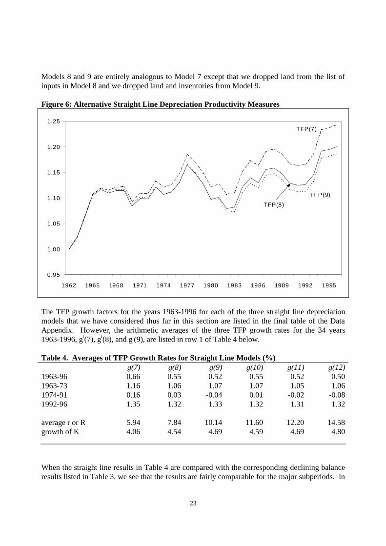
TFP(7) is graphed in Figure 6 below.

Figure 5 Alternative Straight Line Depreciation Aggregate Capital Services Prices

0.0

0.5

1.0

1.5

2.0

2.5

3.0

3.5

4.0

4.5

1962 1965 1968 1971 1974 1977 1980 1983 1986 1989 1992 1995

PK(7)

P K(9)

PK(8)

23

Models 8 and 9 are entirely analogous to Model 7 except that we dropped land from the list ofinputs in Model 8 and we dropped land and inventories from Model 9.

Figure 6: Alternative Straight Line Depreciation Productivity Measures

0.95

1.00

1.05

1.10

1.15

1.20

1.25

1962 1965 1968 1971 1974 1977 1980 1983 1986 1989 1992 1995

TFP(7)

TFP(9)

TFP(8)

The TFP growth factors for the years 1963-1996 for each of the three straight line depreciationmodels that we have considered thus far in this section are listed in the final table of the DataAppendix. However, the arithmetic averages of the three TFP growth rates for the 34 years1963-1996, gt(7), gt(8), and gt(9), are listed in row 1 of Table 4 below.

Table 4. Averages of TFP Growth Rates for Straight Line Models (%)g(7) g(8) g(9) g(10) g(11) g(12)

1963-96 0.66 0.55 0.52 0.55 0.52 0.501963-73 1.16 1.06 1.07 1.07 1.05 1.061974-91 0.16 0.03 -0.04 0.01 -0.02 -0.081992-96 1.35 1.32 1.33 1.32 1.31 1.32

average r or R 5.94 7.84 10.14 11.60 12.20 14.58growth of K 4.06 4.54 4.69 4.59 4.69 4.80

When the straight line results in Table 4 are compared with the corresponding declining balanceresults listed in Table 3, we see that the results are fairly comparable for the major subperiods. In

24

both sets of models, dropping land and then dropping inventories tends to increase the averagegrowth rate of capital services and hence decrease the average rate of TFP growth.. However,the capital service aggregates in the straight line depreciation models tend to grow about .15% to.2% faster than the corresponding declining balance models. This leads to somewhat lower ratesof TFP growth in the straight line models. This effect is particularly pronounced for the “good”years 1992-96: the average TFP growth rate falls from about 1.6% per year for the decliningbalance models to about 1.3 to 1.35% per year for the straight line models. The average realinterest rate for the straight line models increases from 5.94% to 7.84% when land is droppedand to 10.14% when land and inventories are dropped.

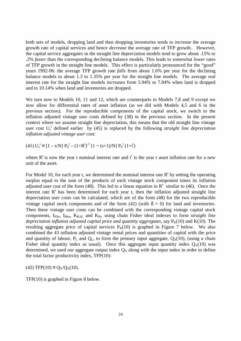
We turn now to Models 10, 11 and 12, which are counterparts to Models 7,8 and 9 except wenow allow for differential rates of asset inflation (as we did with Models 4,5 and 6 in theprevious section). For the reproducible components of the capital stock, we switch to theinflation adjusted vintage user costs defined by (38) in the previous section. In the presentcontext where we assume straight line depreciation, this means that the old straight line vintageuser cost Us

t defined earlier by (45) is replaced by the following straight line depreciationinflation adjusted vintage user cost:

(41) Ust ≡ [1 – s/N] P0

t – (1+Rt)-1 [1 − (s+1)/N] P0t (1+it)

where Rt is now the year t nominal interest rate and it is the year t asset inflation rate for a newunit of the asset. For Model 10, for each year t, we determined the nominal interest rate Rt by setting the operatingsurplus equal to the sum of the products of each vintage stock component times its inflationadjusted user cost of the form (48). This led to a linear equation in Rt similar to (46). Once theinterest rate Rt has been determined for each year t, then the inflation adjusted straight linedepreciation user costs can be calculated, which are of the form (48) for the two reproduciblevintage capital stock components and of the form (42) (with δ = 0) for land and inventories.Then these vintage user costs can be combined with the corresponding vintage capital stockcomponents, INSs, IMes, KBAL and KIS, using chain Fisher ideal indexes to form straight linedepreciation inflation adjusted capital price and quantity aggregates, say PK(10) and K(10). Theresulting aggregate price of capital services PK(10) is graphed in Figure 7 below. We alsocombined the 43 inflation adjusted vintage rental prices and quantities of capital with the priceand quantity of labour, PL and QL, to form the primary input aggregate, QX(10), (using a chainFisher ideal quantity index as usual). Once this aggregate input quantity index QX(10) wasdetermined, we used our aggregate output index QY along with the input index in order to definethe total factor productivity index, TFP(10):

(42) TFP(10) ≡ QY/QX(10).

TFP(10) is graphed in Figure 8 below.

25

Figure 7: Alternative Inflation Adjusted Straight Line Depreciation Aggregate CapitalServices Prices

0.5

1.0

1.5

2.0

2.5

3.0

3.5

4.0

1962 1965 1968 1971 1974 1977 1980 1983 1986 1989 1992 1995

PK(10)

PK(12)

PK(11)

Figure 8: Alternative Inflation Adjusted Straight Line Depreciation Productivity Measures

0.95

1.00

1.05

1.10

1.15

1.20

1.25

1962 1965 1968 1971 1974 1977 1980 1983 1986 1989 1992 1995

TFP(10)

TFP(12)

TFP(11)

26

Models 11 and 12 are entirely analogous to Model 10 except that we dropped land from the listof inputs in Model 11 and we dropped land and inventories from Model 12.

The arithmetic averages of the three straight line depreciation inflation adjusted TFP growth ratesfor the 34 years 1963-1996, gt(10), gt(11), and gt(12), are listed in row 1 of Table 4 above, alongwith the average results for the major subperiods. As was the case with the declining balancemodels described in the previous section, adjusting for inflation tends to reduce average TFPgrowth rates. Thus the average TFP growth rate for the entire period (with all inputs included)falls from .66% per year (Model 7) to .55% per year when we adjusted our straight line vintageuser costs for inflation (Model 10).

We turn now to our gross capital stock models.

6. Alternative Productivity Measures for Canada Using One Hoss Shay Depreciation

Refer back to section 6 above for information on how the vintage capital stocks Ist for each year t

and each vintage s were constructed for each of the two reproducible capital stocks wasconstructed. We now use formula (16) in section 4 to construct the one hoss shay depreciationmodel year t user cost for a reproducible capital stock component. For the nonreproducibleassets, we used the same user costs in Models 13 to 15 as we used in Models 1 to 3 in section 7.

For Model 13, for each year t, we determined the real interest rate rt by setting the operatingsurplus equal to the sum of the products of each vintage stock component times its user cost.This leads to a nonlinear equation in rt of the following form for each year t:

(41) (1+rt)OS = rt [1−(1+rt)-29]-1 PNSt KNS

t + rt [1−(1+rt)-12]-1 PMEt KME

t

+ rt PBALt KBAL

t + rt PISt KIS

t where KNS

t and KMEt are the year t gross capital stocks tabled in section 6 above. The SOLVE

option in SHAZAM was used to solve equation (50) for the real interest rate rt. Once the interestrate rt has been determined for each year t, then the one hoss shay depreciation user costs for eachof the four assets can be calculated, which are of the form (16) for the two reproducible vintagecapital stock components and of the form (30) for land and inventories. Then these user costscan be combined with the corresponding capital stock components, KNS, KME, KBAL and KIS,using chain Fisher ideal indexes to form one hoss shay depreciation capital price and quantityaggregates, say PK(13) and K(13). The resulting aggregate price of capital services PK(13) isgraphed in Figure 9 below. We also combined the one hoss shay rental prices and quantities ofcapital with the price and quantity of labour, PL and QL, to form the primary input aggregate,QX(13), (using a chain Fisher ideal quantity index as usual). Once this aggregate input quantityindex QX(13) was determined, we used our aggregate output index QY along with the input indexin order to define the total factor productivity index, TFP(13):

27

Figure 9: Alternative One Hoss Shay Depreciation Aggregate Capital Services Prices

0.0

0.5

1.0

1.5

2.0

2.5

3.0

3.5

4.0

4.5

1962 1965 1968 1971 1974 1977 1980 1983 1986 1989 1992 1995

PK(13)

PK(15)

PK(14)

Figure 10: Alternative One Hoss Shay Depreciation Productivity Measures

0.95

1.00

1.05

1.10

1.15

1.20

1.25

1962 1965 1968 1971 1974 1977 1980 1983 1986 1989 1992 1995

TFP(13)

TFP(15)

TFP(14)

28

(42) TFP(13) ≡ QY/QX(13).

TFP(13) is graphed in Figure 10.

Models 14 and 15 are entirely analogous to Model 13 except that we dropped land from the listof inputs in Model 14 and we dropped land and inventories from Model 15.

The TFP growth factors for the years 1963-1996 for each of the three one hoss shay depreciationmodels that we have considered thus far in this section are listed in the final table of the DataAppendix. However, the arithmetic averages of the three TFP growth rates for the 34 years1963-1996, gt(13), gt(14), and gt(15), are listed in row 1 of Table 5 below.

Table 5: Averages of TFP Growth Rates for One Hoss Shay and Other Models (%)g(13) g(14) g(15) g(16) g(17) g(18)

1963-96 0.65 0.55 0.52 0.59 0.57 0.961963-73 1.16 1.07 1.08 0.99 1.09 1.031974-91 0.16 0.04 -0.02 0.06 0.05 0.711992-96 1.31 1.26 1.26 1.64 1.33 1.73

average r or R 5.72 7.23 8.76 __ __ __growth of K 4.08 4.55 4.68 4.29 4.43 2.55

When the gross capital stock results in in the first 3 columns of Table 5 are compared with thecorresponding straight line results listed in the first 3 columns of Table 4, we see that the resultsare surprisingly close for the major subperiods. In both sets of models, dropping land and thendropping inventories tends to increase the average growth rate of capital services and hencedecrease the average rate of TFP growth. The only major difference between the first 3 columnsof Tables 4 and the corresponding columns in Table 5 are in the average real interest rates: theytended to be lower in the gross capital stock models.

Differential rates of asset inflation can be introduced into the one hoss shay model ofdepreciation. In the no inflation model of section 4 above, the key equation was (15), which gavethe relationship between the price of a new asset, P0, and its user cost, U0. With a constant rateof inflation expected in future periods, so that the ratio of next period’s new asset price to thisperiod’s price is expected to be (1+i), and with a constant nominal interest rate R, the newrelationship between P0 and U0 is:

(41) P0 = U0 + (1+R)-1(1+i)U0 + (1+R)-2(1+i)2U0 +…+ (1+R)-N+1(1+i)N-1U0

where N is the length of life of a new asset. Equation (52) says that the price of a new assetshould be equal to the discounted stream of future expected rentals. Using (52) to solve for U0 interms of P0 leads to the following inflation adjusted one hoss shay user cost, which replacesformula (16):

29

(42) U0 = P0[(1+R)(1+i)-1 – 1](1+i)(1+R)-1[1 – (1+R)-N(1+i)N]-1. It is now possible to repeat Models 13-15, using the inflation adjusted user costs defined by (53)for the reproducible capital stock components in place of the earlier user cost formula (16).However, given the nonlinearity of (53), we did not follow this path. If the one hoss shay modelof depreciation were true, then annual rental and leasing rates for reproducible assets would beconstant across vintages at any given point in time. Thus an old asset would rent for the sameprice as a new asset. This does not seem to be consistent with the “facts” and thus we do notbelieve it is worth spending a lot of time on one hoss shay models. We conclude this empirical part of our paper by computing two additional capital servicesaggregates. For our first additional capital aggregate, we took our declining balance estimates forthe two reproducible capital stock components tabled in section 6 above, KNS and KME, andformed a chained Fisher ideal aggregate of these two stocks, using the investment prices PNS andPME as price weights in the index number formula. We then divided the resulting stockaggregate, K(16) say, into the operating surplus OS to obtain a corresponding implicit price,PK(16) say. PK(16) is graphed in Figure 11 below, along with our first declining balanceaggregate capital services price PK(1) for comparison purposes. We then combined this capitalaggregate with the price and quantity of labour, PL and QL, in another chained Fisher idealaggregation in order to form an input aggregate, QX(16). Note that land and inventory stocks areomitted from this input aggregate. Once this aggregate input quantity index QX(16) wasdetermined, we used our aggregate output index QY along with this input index in order to definethe total factor productivity index, TFP(16):

(43) TFP(16) ≡ QY/QX(16). TFP(16) is graphed in Figure 12 below along with our first declining balance total factorproductivities, TFP(1), for comparison purposes. For our second additional capital aggregate, we took our gross capital stock estimates for the tworeproducible capital stock components tabled in section 6 above and formed a chained Fisherideal aggregate of these two stocks, using the investment prices PNS and PME as price weights inthe index number formula. We then divided the resulting stock aggregate, K(17) say, into theoperating surplus OS to obtain a corresponding implicit price, PK(17) say. PK(17) is graphed inFigure 11 below. We then combined this capital aggregate with the price and quantity of labour,PL and QL, in another chained Fisher ideal aggregation in order to form an input aggregate,QX(17). Note that land and inventory stocks are omitted from this input aggregate. Once thisaggregate input quantity index QX(17) was determined, we used our aggregate output index QY

along with this input index in order to define the total factor productivity index, TFP(17):

(44) TFP(17) ≡ QY/QX(17).

30

Figure 11: Some Capital Services Price Aggregates

0.0

0.5

1.0

1.5

2.0

2.5

3.0

3.5

4.0

4.5

1962 1965 1968 1971 1974 1977 1980 1983 1986 1989 1992 1995

PK(1)

P K(16)

PK(17)

Figure 12: Additional Productivity Measures

0.95

1.00

1.05

1.10

1.15

1.20

1.25

1.30

1.35

1.40

1962 1965 1968 1971 1974 1977 1980 1983 1986 1989 1992 1995

TFP(18)

TFP(1)

TFP(16)

TFP(17)

31

TFP(17) is graphed in Figure 12. It can be seen that these last two TFP concepts (with ‘incorrect’weighting) lead to a somewhat slower rate of TFP improvement over the entire sample comparedto the no inflation declining balance concept, TFP(1).

Our final miscellaneous productivity measure is labour productivity TFP(18) defined as ouroutput aggregate QY divided by our measure of labour input QL.17 It is graphed in Figure 12.The final column in Table 5 shows that the average labour productivity growth rate over the 34years in our sample was .96% per year which is almost twice as big as our typical average TFPgrowth rate. However, by international standards, this is a rather low rate of growth for labourproductivity.

The average rates of TFP growth for our “incorrectly” weighted declining balance productivitymeasure TFP(16) and our “incorrectly” weighted gross capital stock productivity measureTFP(17) for the entire sample period was .59% per year and .57% per year respectively; seecolumns 4 and 5 in Table 5 above. These average growth rates are between those for the noinflation declining balance Models 1 and 3 (.68% and .55%) and the no inflation gross stockModels 13 and 15 (.65% and .52%). Thus our incorrectly weighted models led to productivityestimates that were fairly close to the estimates from the “correctly” weighted models.

10. Conclusion

We have shown that neglecting land and inventories leads to a decline in average TFP growthrates in Canada of about .1% per year, which is not large in absolute terms, but is large in relativeterms, since the average growth rate for total factor productivity in Canada only averaged .5 to.6% per year over the years 1963-96. However, once land and inventories are included in thecapital aggregate, the differences in average TFP growth rates between the various depreciationmodels (declining balance, one hoss shay and straight line) proved to be surprisingly small,whether we allowed for differential rates of asset inflation or not.

We summarize our results in Figure 13, where we graph our productivity estimates for Model 1(declining balance depreciation including all assets), Model 4 (declining balance depreciationincluding all assets with inflation adjustments), Model 7 (straight line depreciation including allassets), Model 10 (straight line depreciation including all assets with inflation adjustments),Model 13 (one hoss shay depreciation including all assets), Model 16 (declining balancedepreciation but with “incorrect” stock weights instead of user cost weights and excluding landand inventories) and Model 17 (one hoss shay depreciation but with “incorrect” stock weightsinstead of user cost weights and excluding land and inventories). It can be seen that the three‘correctly’ weighted models with no inflation were relatively close to each other and finished upabout 5 percentage points higher than the two ‘correctly’ weighted models with inflationadjustments, TFP(4) and TFP(10), and the two ‘incorrectly’ weighted measures, TFP(16) andTFP(17). We note the highest estimate of TFP in 1996 is given by Model 1 (a 25.29% increase

17 This measure was normalized to equal 1 in 1962.

32

from 1962) and the lowest estimate is given by Model 10 (a 19.63% increase). This is not a hugerange of variation.

Figure 13: Alternative Total Factor Productivity Estimates for Canada

0.95

1.00

1.05

1.10

1.15

1.20

1.25

1962 1965 1968 1971 1974 1977 1980 1983 1986 1989 1992 1995

TFP(1)

TFP(13)

TFP(7)

TFP(17)

TFP(10)TFP(16)

TFP(4)

All of our productivity estimates paint more or less the same dismal picture of Canada’sproductivity performance. During the pre OPEC years, 1962-73, TFP growth proceeded at thesatisfactory rate of about 1 per cent per year. Then for the 18 “lost” years, 1974-1991, TFPgrowth was close to 0 on average. Fortunately, there appears to have been a strong TFP recoveryin recent years; TFP growth averaged somewhere between 1.6% and 1.3% per year for the 5years 1992-96.18

There are many problems associated with the measurement of capital that were not discussed inthis paper. Some of these problems are:

• We have discussed only ex post user costs, which we think is appropriate when measuringthe productivity performance of a firm or industry or country. However, for many otherpurposes (such as econometric modeling), ex ante or expected user costs are more relevant.

18 Diewert and Fox (1999) hypothesized that the world wide TFP slowdown that occurred in OECD countries around1973 was probably related to the big increase in inflation that occurred around that time. Inflation was high inCanada during the years 1974-1991 and then low in recent years. Thus Canada’s recent productivity recovery isconsistent with the Diewert and Fox hypothesis.

33

• The user costs that were defined neglected the complications due to the business income taxand other taxes on capital. Essentially, our user costs assume that these taxes just reduce thepretax real or nominal rate of return.19

• We have not related depreciation to the utilisation of the asset.• We have discussed only the easy to measure components of the capital stock. Other

components that were not discussed include resource stocks, knowledge stocks andinfrastructure stocks.

• We have not modeled the role of research and development expenditures and of knowledgespillovers.

• We have not discussed the problems involved in measuring capital when there are qualityimprovements in new units of the capital stock.

However, we hope that our presentation of alternative models of depreciation will be helpful tobusiness and academic economists who find it necessary to construct capital aggregates in thecourse of their research. We also hope that our exposition will be helpful to statistical agencieswho may be contemplating adding a productivity module to their economic statistics. We haveshown that it is relatively easy to do this once accurate information on asset lives (or decliningbalance depreciation rates) are available.

19 Thus our rt or Rt are returns that include these business taxes.

34

Data Appendix

In this appendix, we will briefly describe our sources and list the data actually used in our capitalstock and productivity computations.

We begin by describing the construction of our aggregate output variable. From Tables 52 and53 of the Statistics Canada publication, National Income and Expenditure Accounts, AnnualEstimates 1984-1995 (and other years), we were able to construct consistent estimates for 19categories of consumer expenditures for the years 1962-1996. The 19 categories were: (1) foodand nonalcoholic beverages; (2) alcoholic beverages; (3) tobacco products; (4) clothing, footwearand accessories; (5) electricity, natural gas and other fuels; (6) furniture, carpets and householdappliances; (7) semidurable household furnishings plus reading and entertainment supplies; (8)nondurable household supplies, drugs and sundries, toilet articles and cosmetics; (9) medicalcare, hospital care and other medical care expenses; (10) new and (net) used motor vehicles plusmotor repairs and parts; (11) motor fuels and lubricants; (12) other auto related services pluspurchased transportation; (13) communications; (14) recreation equipment, jewelry, watches andrepairs; (15) recreational services; (16) educational and cultural services; (17) financial, legal andother services; (18) expenditures on restaurants and hotels and (19) other services (laundry anddry cleaning, domestic and child care services, other household services and personal care). Notethat we do not include consumption of housing services in the above list of consumer goods andservices. We will also exclude the stock of dwellings from our list of market sector capitalinputs. The price series for the above 19 components of consumer expenditure contain variouscommodity taxes, which are revenues for government but are not revenues for private producers.Thus we attempted to remove these commodity taxes from the above price series usinginformation contained in the Statistics Canada publication, The Input-Output Structure of theCanadian Economy 1961-1981 and other years. Additional information from the StatisticsCanada publication, The Canadian Economic Observer for May 1989 and other Statistics Canadasources was used in order to construct final estimates of commodity taxes for the above 19 finaldemand consumption categories. We note that we were unable to allocate all indirect taxes andsubsidies to the appropriate categories so our market sector output aggregate will be subject tosome measurement error.

We turn now to a description of our international trade data. It should be mentioned that ourtreatment of international trade follows that of Kohli (1978)(1991). In this treatment, exports areproduced by the market sector and all imports flow into the market sector as intermediate inputs.These import inputs are either physically transformed by domestic producers or they havedomestic value added to them through domestic transportation, storage or retailing activities.When we construct our market sector output aggregate, we index import quantities with anegative sign in keeping with national income accounting conventions.

In forming consistent series for disaggregated export and import components, the principal datasource was the Statistics Canada CANSIM matrices 6566 and 6541. These matrices providecurrent and constant price series for 11 export and 11 import components for the years 1971 to1993.

35

For exports, the 11 components were aggregated into the following 5 categories on the basis ofsimilarities in price movements (Hicks aggregation): (1) Forestry; (2) Energy; (3) Equipment;(4) Other goods; and (5) Services. The Forestry and Energy categories were formed directly fromthe equivalent CANSIM series. The Equipment category is an aggregate of the CANSIM seriesfor Machinery and equipment and Automotive products. The residual Other goods exportscategory is an aggregate of the CANSIM Agricultural and fish products, Industrial goods andmaterials and Other consumer goods components. The Services category is an aggregate of theCANSIM Travel services, Transportation services and Commercial services components plus thevalue of Government services obtained from Statistics Canada’s Canada’s Balance ofInternational Payments, 1926 to 1996 and first quarter 1997, Catalogue No. 67-001-XPB, Table13. The Government services variable mainly comprises expenditures by foreign governments inCanada. It is excluded from the CANSIM series but we assume these purchases are from theCanadian business sector and so should be included in our export series. The eleventh CANSIMcomponent – Financial Intermediation services – was omitted, as it does not accurately representthe movement of goods or services. Rather, it is largely a financial balancing item. Export priceindexes were formed using chained Fisher indexes of the component implicit prices from theCANSIM current and constant price matrices. As our complete database runs over the years1962 to 1996, we had to backdate our 5 export categories to 1962 using a variety of sources. Inorder to extend the CANSIM series from 1993 to 1996, again a variety of sources were used.The values and prices of exports of the four goods components were updated from 1993 to 1996using Statistics Canada’s Canadian Economic Observer, Catalogue No. 11-010-XPB, Tables 18and 19. The July 1996 and November 1997 issues spanned the four year period. Values andcurrent weighted price indexes were presented for exports of Agriculture and fish, Energy,Forestry, Industrial goods and materials, Machines and equipment, Automotive and Consumergoods. The value of the four services items making up the Services export component wereupdated from Statistics Canada’s Canada’s Balance of International Payments, 1926 to 1996 andfirst quarter 1997, Catalogue No. 67-001-XPB, Table 13. The price of the overall Services exportcomponent was updated to 1996 using the price of non-merchandise exports obtained fromCANSIM matrix 6628, Current and constant dollar estimates of non-merchandise exports andimports from the National Accounts.

The values and price indexes for the five export categories described above are measured at theborder and so exclude export taxes paid by producers. To derive exports in producers’ prices weneeded to estimate export taxes for each of our five export components. The only exportcomponents, which had significant export taxes, are Energy and Services exports. Between 1973and 1985 Canada imposed an Oil Export Charge. Values of this tax were obtained from StatisticsCanada’s National Income and Expenditure Accounts, Annual Estimates, 1926-83, CatalogueNo. 13-531, Table 51. For Services exports, we assumed that three of its components were taxed:Travel, Freight and shipping, and Government services. We assumed that Travel andGovernment services exports were each made up of half expenditure on fuel and half expenditureon hotels and restaurants. Consequently, the commodity tax rates for Fuel and Hotels andrestaurants were each applied to half the expenditure in each of these components. We assumedthat half of Freight and shipping exports were made up of fuel expenses and subject to thecommodity tax rate for Fuel. Other services exports were assumed not to be taxed.

36

For imports, the 11 components in CANSIM matrices 6566 and 6541 were aggregated into thefollowing 4 categories on the basis of similarities in price movements (Hicks aggregation): (1)Forestry and other; (2) Energy; (3) Equipment; and (4) Services. The Energy and Equipmentcategories are formed directly from the equivalent CANSIM series. The Services category is anaggregate of the Travel, Transportation and Commercial services components. The Forestry andother imports category is the aggregate of the Forestry, Agricultural and fish products, Industrialgoods and materials, Automotive products and Other consumer goods components. FinancialIntermediation services are again omitted. Import price indexes were formed using chainedFisher indexes of the component implicit prices from the CANSIM current and constant pricematrices. As was the case with exports, our 4 import series were backdated to 1962 using avariety of sources. The values and prices of imports of the three goods components were updatedfrom 1993 to 1996 using Statistics Canada’s Canadian Economic Observer, Catalogue No. 11-010-XPB, Tables 18 and 19. The July 1996 and November 1997 issues spanned the four yearperiod. Values and current weighted price indexes were presented for imports of Agriculture andfish, Energy, Forestry, Industrial goods and materials, Machines and equipment, Automotive andConsumer goods. The value of the three services items making up the Services importcomponent were updated from Statistics Canada’s Canada’s Balance of International Payments,1926 to 1996 and first quarter 1997, Catalogue No. 67-001-XPB, Table 13. The price of theoverall Services import component was updated to 1996 using the price of non-merchandiseimports obtained from CANSIM matrix 6628, Current and constant dollar estimates of non-merchandise exports and imports from the National Accounts. These import values and pricesare measured at the border and so exclude import duties. To derive imports in producers’ priceswe needed to estimate import duties for each of our four import components. Total import dutiesfor the period 1962-83 were obtained from Statistics Canada’s National Income and ExpenditureAccounts, Annual Estimates, 1926-83, Catalogue No. 13-531, Table 51. Import duties for 1984-95 were obtained from National Income and Expenditure Accounts, 1984-95, Catalogue No. 13-201-XPB, Table 44. Total import duties for 1996 were estimated by assuming the same aggregatetariff rate applied as that observed in 1995. An estimate of the duty paid on Equipment importswas obtained from various issues of the Canadian Tax Foundation’s The National Finances forthe years 1964-85. The following categories from the End products, inedible, category wereallocated to Equipment imports: General purpose industrial machinery, Special industrymachinery, Road motor vehicles, Communication and related equipment, Electric lighting,distribution and control equipment and Office machines and equipment. Values for 1969, 1974and 1984 were estimated by interpolating implied tariff rates. Equipment import duties for theremaining periods, 1962-63 and 1986-96, were estimated by linking the implied Equipment tariffrate to movements in the total imports implied tariff rate. Information in The National Financesindicated there were no import duties on Energy imports. We assume there are no tariffs applyingto Services imports so the remaining duties are allocated to the Forestry and other importscomponent. Between 1973 and 1985 Canada subsidized oil imports. The amount of the OilImport Compensation Charge was obtained from The National Finances. This enters as asubsidy, or negative tax, on Energy imports for these years. The subsidy rate for 1982 appearedanomalous and was replaced by an interpolated rate.

37

The government purchases intermediate inputs and investment goods from the market sector so itis necessary to form estimates for these components of market sector output. We have data on thevalue and price of total government consumption and government wages payments from theOECD Economic Outlook database (Econdata 1997). We derive the value of governmentpurchases of intermediates by subtracting government wages payments from total governmentconsumption. Having derived the value and price of government purchases of intermediates, wecombine this with the value and price of government investment in fixed capital from CANSIMmatrices 6828 and 6836, respectively, using a chain Fisher index. Our next task was to deriveproducers’ price series for the two components of government purchases. Indirect taxes paid ontotal government purchases from the market sector (both intermediates and fixed capitalexpenditure) were obtained from the final demand matrices of Statistics Canada’s Input–OutputTables for the years 1962 to 1992. An indirect tax rate was formed by taking the ratio of indirecttaxes paid to the value of total government purchases from the market sector. The tax rate for1992 was assumed to also apply for the remaining four years, 1993 to 1996. Producers’ priceindexes were then formed by multiplying the government intermediates and investment priceindexes by one minus the indirect tax rate.

The final components of our market sector output aggregate are the investment components andthe change in inventories. From The Canadian Economic Observer, Historical StatisticalSupplement, 1997/98, we obtained investment in nonresidential structures and in machinery andequipment in current and constant dollars for the years 1962-1997. The resulting price (PNS andPME) and quantity series (INS and IME) are listed in Table A1 below.

The construction of price and quantity series for inventory change is not straightforward. FromThe Canadian Economic Observer, Historical Statistical Supplement, 1997/98, we obtainedestimates of inventory in current and constant dollars for the years 1962-1997. The resultingprice series is listed in Table A1 below as PINA (price of inventories using national accounts data).It can be seen that this price series for inventory change is not credible as a measure of theaverage level of inventory prices in a given year. Hence, we will use the Statistics CanadaNational Balance Sheet Accounts, Annual Estimates, 1996 for estimates of the total stock ofinventories (in current dollars) held at the end of the year for the years 1964 to 1996. This in turnis equal to the beginning of the year stock of inventories held by the market sector (thegovernment’s holdings of inventories was negligible) for the years 1965-1997. This series can beextended back to stocks held at the beginning of 1962 using the National Balance Sheet Accountsfor an earlier year. Constant dollar stocks of inventories are available for the end of years 1961-1982 from the National Balance Sheet Accounts, Annual Estimates, 1984 and for the end of years1984-1993 from the National Balance Sheet Accounts, Annual Estimates, 1994. The resultingbeginning of the year inventory stock price and quantity series for the years 1962-1994 are listedin Table A1 as PIS and KIS. In order to extend our inventory price series to 1997, we linked PIS tothe (erratic) national accounts series PINA at the year 1992, which was the base year for theconstant dollar inventory change series. The final 3 entries in the PIS series reflect this linkingprocedure. The resulting PIS series looks quite reasonable. Of course, once we have our priceseries for beginning of the year inventory stocks, PIS, it can be divided into the balance sheetvalue estimates to obtain the quantity series for beginning of the year inventory stocks, KIS, for

38

all 37 years in our sample, 1962-1997. Once KIS has been determined, then inventory change,QIC for the 36 years 1962-1996 can be obtained by differencing the stock series, KIS.

Table A1: Market Sector Output Data for Canada; 1962-1997Year PNS PME PIS PINA PY

1962 1.0000 1.0000 1.0000 1.0000 1.00001963 1.0285 1.0280 0.9866 0.9918 1.02411964 1.0579 1.0695 1.0288 1.0909 1.04561965 1.1168 1.1114 1.0451 1.0445 1.08421966 1.1843 1.1476 1.0718 1.0325 1.14221967 1.2355 1.1398 1.0970 1.0960 1.17971968 1.2492 1.1387 1.1180 1.1506 1.23061969 1.3199 1.1692 1.1376 1.0938 1.29361970 1.3872 1.2245 1.1618 1.3038 1.34951971 1.4713 1.2576 1.1638 1.0937 1.40271972 1.5549 1.3077 1.1830 1.2551 1.48001973 1.7235 1.3433 1.2974 1.3728 1.62121974 2.0439 1.4864 1.5420 1.4454 1.87761975 2.2837 1.6650 1.8820 1.7817 2.10211976 2.4139 1.7641 1.9290 1.7078 2.27731977 2.5428 1.8706 1.9544 2.0536 2.40251978 2.7279 1.9467 2.0555 1.6277 2.56871979 2.9751 2.0667 2.2834 1.8909 2.85541980 3.3367 1.9616 2.6506 4.2658 3.20141981 3.7133 1.9860 3.0073 2.5485 3.56561982 3.9903 2.1330 3.2945 2.7584 3.86871983 3.9631 2.1127 3.3440 2.7320 4.06071984 4.1112 2.0873 3.4455 2.9947 4.17191985 4.2349 2.0339 3.5308 2.4212 4.25711986 4.2977 2.0313 3.5633 2.8847 4.30851987 4.4991 1.9851 3.6102 2.7174 4.48811988 4.7563 1.9477 3.7149 4.4340 4.66041989 4.9655 1.9397 3.8702 2.8741 4.87201990 5.1192 1.9237 3.8954 4.2322 5.01211991 5.0094 1.7483 3.8846 3.1432 5.09851992 4.9730 1.6926 3.7546 3.1024 5.11141993 5.0365 1.7181 3.9027 3.9837 5.14311994 5.2066 1.7630 4.0362 2.2776 5.21641995 5.2717 1.7845 4.1109 3.3968 5.35851996 5.2479 1.7719 4.1564 3.4343 5.49991997 4.0474 3.3443

39

Table A1: Market Sector Output Data for Canada; 1962-1997 (cont’d)Year INS IME KIS QIC QY

1962 2560.0 2368.0 13811.3 791.8 32312.71963 2647.5 2570.1 14603.1 467.5 33750.71964 3060.7 3023.8 15070.7 461.1 36237.11965 3338.2 3551.4 15531.8 1145.3 38933.81966 3830.9 4229.7 16677.1 1176.2 41905.01967 3631.8 4321.8 17853.4 352.7 43435.41968 3601.6 4022.9 18206.1 759.0 44962.31969 3605.6 4404.0 18965.1 1579.5 46565.01970 3955.5 4489.0 20544.6 376.3 48619.91971 4080.2 4623.2 20920.9 316.5 50250.71972 4063.3 4999.5 21237.5 120.1 51961.91973 4384.0 6119.1 21357.5 428.7 55649.01974 4652.5 6893.1 21786.2 1546.0 57391.41975 5261.6 7285.4 23332.3 650.7 59005.11976 5139.9 7603.2 23982.9 1553.2 62302.41977 5450.6 7584.9 25536.1 2033.7 65853.21978 5591.9 8207.6 27569.8 1059.5 67678.31979 6311.6 9550.6 28629.3 1436.1 69943.61980 7030.7 11527.5 30065.5 -907.5 70814.51981 7565.8 13936.2 29157.9 450.0 73641.71982 6877.9 11750.8 29608.0 -2476.4 71606.81983 6309.2 11531.0 27131.5 -670.5 72619.01984 6242.5 12306.7 26461.1 1428.8 77445.11985 6556.9 14174.9 27889.8 790.5 81153.71986 6177.5 15712.8 28680.4 570.6 83345.01987 6416.4 18135.8 29251.0 929.3 87498.11988 7067.9 21512.3 30180.3 699.7 91071.21989 7285.1 23169.5 30880.0 1180.8 92786.71990 7302.0 22141.5 32060.7 -569.0 92968.81991 7065.7 22260.9 31491.8 -613.4 91988.51992 5962.9 22836.3 30878.4 -1149.9 92059.51993 5992.9 21725.6 29728.5 357.6 95077.81994 6521.2 23719.6 30086.1 1820.7 100532.21995 6473.1 25129.9 31906.8 2051.4 103633.51996 6752.6 26179.2 33958.2 1696.2 104886.01997 35654.4

This completes our description of the construction of the components of our market sector outputaggregate. The aggregate price of output, PY, and the aggregate quantity of output, QY, wereconstructed as chained Fisher ideal indexes of the 19 consumption components, the 5 exportcomponents, the 4 import components, the 2 government components (investment purchases and

40

purchases of goods and services), the 2 investment components and the inventory changecomponent. PY and QY are listed in Table A1.

We now describe the construction of the primary input components for the market sector of theCanadian economy.

We first describe our labour estimates. From The Canadian Economic Observer, HistoricalStatistical Supplement, 1997/98, we obtained estimates of the number of self employed workers(including unpaid family workers) from Table 8. For the years 1962-1974, we obtained the sameinformation from various Canada Year Books. For the year 1975, we interpolated an estimateusing the two sources. From Table 9 of The Canadian Economic Observer, Historical StatisticalSupplement, 1997/98, we obtained estimates of total labour income and labour income paid outto public administration workers. Thus by subtraction, we obtained estimates for market sectoremployment income. From the Organisation of Economic Cooperation and Development’sEconomic Outlook database (Econdata 1997), we obtained data on the business compensationrate, PL, which is an annual wage that reflects the full cost of employing a full time worker. Weattributed 2/3 of this annual wage rate to the self employed and we assume that all of the selfemployed worked in the market sector rather than the government sector. This gave us a new(bigger) estimate of market sector total labour income. We divided this labour value series bythe full time market wage rate PL in order to obtain market sector labour input, QL. The series PL

and QL are listed in Table A2. Subtracting PL times QL from the value of market sector outputs(less imports), PY times QY, gave us estimates of the market sector’s operating surplus, OS. Thisseries is also listed in Table A2.

We turn now to the capital components of the input aggregate. We have already described howwe used the National Balance Sheet Accounts for estimates of the total stock of inventories. Thesame balance sheets can be used to form estimates of the beginning of the year stocks ofnonresidential structures, machinery and equipment and land used by the market sector. We willnot go through all of the details of the construction of these series. These beginning of the yearbalance sheet estimates for constant 1962 dollar net nonresidential structures stocks, KNS,machinery and equipment stocks, KME, and business and agricultural land stocks, KBAL, are listedin Table A2 below along with the corresponding price of land, PBAL. Note that we have assumedthat the stock of business and agricultural land is constant. The price for a unit of thenonresidential structures is assumed to be the same as the corresponding investment price, PNS.The price for a unit of the machinery and equipment stock is assumed to be the same as thecorresponding investment price, PME.20

20 We could have used the price deflators for nonresidential structures and for machinery and equipment that can beconstructed using the constant dollar estimates of these stock components that may be found in the National BalanceSheet Estimates. However, we found that the resulting balance sheet price series for machinery and equipmentdiffered substantially from the corresponding investment price deflator for machinery and equipment listed in TableA1, PME. We feel that the investment price and quantity data are more accurate than the balance sheet price andquantity data with the exception of the national accounts change in inventories series. Thus we used the nationalaccounts investment prices PNS and PME to deflate the balance sheet capital stock values for nonresidential structuresand machinery and equipment repectively.

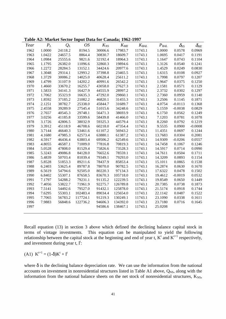
41

Table A2: Market Sector Input Data for Canada; 1962-1997Year PL QL OS KNS KME KBAL PBAL δNS δME

1962 1.0000 24118.2 8194.5 30006.6 17983.7 11743.1 1.0000 0.0578 0.09691963 1.0422 24657.5 8864.4 30830.7 18609.7 11743.1 1.0695 0.0417 0.11911964 1.0984 25555.6 9821.6 32192.4 18964.3 11743.1 1.1647 0.0743 0.11041965 1.1795 26382.0 11096.6 32860.3 19894.6 11743.1 1.3126 0.0540 0.12411966 1.2272 28284.5 13152.1 34424.6 20977.6 11743.1 1.4529 0.0249 0.08301967 1.3048 29314.1 12993.2 37398.8 23465.5 11743.1 1.6315 0.0108 0.09271968 1.3729 30086.2 14025.0 40628.4 25611.2 11743.1 1.7998 0.0797 0.12071969 1.4799 31107.9 14202.2 40991.6 26542.2 11743.1 1.9647 0.0375 0.12501970 1.4660 33670.2 16255.7 43058.0 27627.3 11743.1 2.1581 0.0571 0.11291971 1.5833 34141.3 16427.9 44555.9 28997.2 11743.1 2.3732 0.0302 0.12971972 1.7062 35323.9 16635.3 47292.0 29860.1 11743.1 2.7360 0.0959 0.11401973 1.8592 37185.2 21082.2 46820.1 31455.3 11743.1 3.2506 0.1145 0.18711974 2.1251 38782.7 25338.0 45844.7 31689.7 11743.1 4.0754 -0.0113 0.13681975 2.4558 39289.9 27545.4 51015.6 34248.6 11743.1 5.1559 -0.0038 0.08291976 2.7657 40545.3 29748.1 56471.3 38693.9 11743.1 6.1750 0.0562 0.12491977 3.0256 41185.8 33599.6 58439.8 41466.0 11743.1 7.1203 0.0781 0.10781978 3.1726 42806.5 38032.9 59325.3 44579.4 11743.1 8.2260 0.0792 0.12191979 3.3912 45118.9 46708.6 60218.0 47354.4 11743.1 9.5535 0.0900 -0.00081980 3.7144 46640.3 53461.6 61107.2 56943.2 11743.1 11.4351 0.0697 0.12441981 4.1680 47985.3 62573.4 63880.1 61387.2 11743.1 13.7683 0.0304 0.20811982 4.5917 46436.4 63803.4 69506.2 62549.6 11743.1 14.9309 -0.0206 0.05571983 4.8055 46587.1 71009.0 77816.8 70819.3 11743.1 14.7458 0.1067 0.12461984 5.0528 47808.0 81529.4 75826.6 73528.3 11743.1 14.5917 0.0714 0.09901985 5.3243 49086.8 84128.0 76652.6 78559.1 11743.1 14.7611 0.0504 0.17111986 5.4839 50703.4 81039.4 79349.1 79293.0 11743.1 14.3209 0.0893 0.11541987 5.8528 51853.3 89211.6 78437.9 85853.4 11743.1 15.1011 0.0865 0.15381988 6.2403 53625.4 89787.8 78070.0 90782.5 11743.1 16.2874 0.0630 0.16701989 6.5619 54794.6 92505.0 80220.3 97134.3 11743.1 17.6322 0.0478 0.15021990 6.8402 55307.1 87658.5 83670.3 105718.0 11743.1 19.4612 -0.0019 0.05321991 7.1797 54288.2 79231.1 91135.2 122239.5 11743.1 19.8549 0.0650 0.14491992 7.4056 53822.7 71961.9 92275.7 126789.8 11743.1 20.7385 0.0738 0.18731993 7.5141 54492.6 79527.0 91432.1 125878.0 11743.1 21.5174 0.0918 0.17441994 7.6295 55303.1 102483.4 89034.4 125654.0 11743.1 22.1142 0.0487 0.15221995 7.7065 56783.2 117724.1 91219.3 130249.1 11743.1 23.1090 0.0338 0.16111996 7.9883 56848.6 122736.2 94606.3 134392.0 11743.1 23.7180 0.0716 0.16451997 94586.6 138467.1 11743.1 25.0208

Recall equation (13) in section 3 above which defined the declining balance capital stock interms of vintage investments. This equation can be manipulated to yield the followingrelationship between the capital stock at the beginning and end of year t, Kt and Kt+1 respectively,and investment during year t, It:

(A1) Kt+1 = (1-δ)Kt + It

where δ is the declining balance depreciation rate. We can use the information from the nationalaccounts on investment in nonresidential structures listed in Table A1 above, QNS, along with theinformation from the national balance sheets on the net stock of nonresidential structures, KNS,

42

and use equation (A1) to construct implied geometric depreciation rates, δNS, that are consistentwith the two data sources. Similarly, we can use the information from the national accounts oninvestment in nonresidential structures listed in Table A1 above, QME, along with the informationfrom the national balance sheets on the net stock of nonresidential structures, KME, from TableA2 and use equation (A1) to construct implied geometric depreciation rates, δME, that areconsistent with the two data sources.

Table A3: Productivity Growth Rates (%) for 18 Capital Models for CanadaYear g(1) g(2) g(3) g(4) g(5) g(6) g(7) g(8) g(9)1963 2.20 2.13 2.25 2.14 2.11 2.25 2.18 2.13 2.261964 3.96 3.89 3.92 3.91 3.89 3.92 3.99 3.94 3.991965 4.02 3.92 3.89 3.95 3.92 3.88 4.14 4.05 4.051966 0.99 0.84 0.92 0.85 0.81 0.90 1.16 1.02 1.121967 -0.59 -0.77 -0.75 -0.77 -0.79 -0.77 -0.39 -0.56 -0.531968 0.38 0.26 0.15 0.28 0.25 0.14 0.50 0.39 0.291969 0.09 -0.02 -0.01 0.03 -0.02 -0.02 0.14 0.04 0.051970 -2.65 -2.78 -2.66 -2.78 -2.82 -2.67 -2.60 -2.72 -2.601971 1.39 1.30 1.23 1.32 1.31 1.22 1.45 1.35 1.291972 -0.07 -0.15 -0.21 -0.18 -0.15 -0.22 -0.02 -0.10 -0.161973 2.14 2.06 1.97 2.01 2.01 1.94 2.19 2.10 2.021974 -1.19 -1.31 -1.39 -1.39 -1.39 -1.42 -1.10 -1.23 -1.311975 0.55 0.39 0.43 0.32 0.40 0.43 0.52 0.36 0.391976 1.86 1.72 1.65 1.67 1.76 1.66 1.83 1.70 1.621977 3.31 3.17 3.19 3.10 3.15 3.19 3.29 3.14 3.161978 -1.28 -1.42 -1.36 -1.44 -1.43 -1.38 -1.30 -1.45 -1.391979 -1.74 -1.88 -1.90 -1.96 -1.94 -1.95 -1.72 -1.86 -1.891980 -2.49 -2.68 -2.71 -2.82 -2.79 -2.80 -2.45 -2.64 -2.671981 0.48 0.30 0.01 0.24 0.16 -0.04 0.52 0.34 0.041982 -1.82 -2.04 -2.19 -1.85 -2.07 -2.20 -1.75 -1.98 -2.141983 0.37 0.30 -0.02 0.32 0.23 -0.04 0.28 0.20 -0.131984 3.87 3.78 3.63 3.85 3.74 3.60 3.73 3.64 3.481985 1.90 1.76 1.81 1.90 1.74 1.79 1.77 1.64 1.691986 -0.69 -0.81 -0.83 -0.72 -0.84 -0.87 -0.73 -0.84 -0.871987 2.34 2.24 2.20 2.20 2.15 2.11 2.31 2.22 2.181988 0.46 0.35 0.33 0.30 0.25 0.23 0.45 0.35 0.331989 -0.90 -1.01 -1.06 -1.08 -1.09 -1.14 -0.88 -0.99 -1.031990 -1.56 -1.65 -1.67 -1.77 -1.75 -1.77 -1.57 -1.67 -1.681991 -0.23 -0.28 -0.34 -0.37 -0.35 -0.40 -0.31 -0.35 -0.411992 0.52 0.51 0.48 0.50 0.51 0.48 0.17 0.14 0.101993 2.01 2.01 1.99 2.00 1.99 1.98 1.71 1.70 1.661994 4.33 4.32 4.32 4.33 4.32 4.32 4.06 4.04 4.041995 0.58 0.54 0.59 0.57 0.54 0.59 0.33 0.28 0.331996 0.69 0.63 0.71 0.65 0.62 0.71 0.48 0.42 0.49

43

The resulting depreciation rates are listed in Table A2. Although the arithmetic averages of theseannual geometric depreciation rates ( .0555 for nonresidential structures and .1256 for machineryand equipment) are very reasonable, it can be seen that the annual fluctuations in these rates areunacceptably large. Thus we regard the balance sheet estimates for the net capital stocks for thetwo reproducible capital stock components, KNS and KME, as being “correct” over the entiresample period but not in the year to year movements.

Table A3: Productivity Growth Rates (%) for 18 Capital Models for Canada (cont’d)Year g(10) g(11) g(12) g(13) g(14) g(15) g(16) g(17) g(18)1963 2.12 2.10 2.25 2.08 2.01 2.10 2.22 2.07 2.171964 3.95 3.94 3.99 3.90 3.84 3.85 3.90 3.83 3.591965 4.08 4.07 4.06 4.11 4.03 4.02 3.89 4.01 4.081966 1.04 1.01 1.12 1.20 1.08 1.18 0.95 1.19 0.391967 -0.56 -0.57 -0.54 -0.29 -0.42 -0.36 -0.69 -0.34 0.011968 0.41 0.38 0.28 0.55 0.45 0.38 0.20 0.40 0.861969 0.08 0.04 0.05 0.15 0.05 0.06 0.00 0.07 0.161970 -2.72 -2.76 -2.61 -2.58 -2.69 -2.57 -2.63 -2.56 -3.531971 1.38 1.38 1.28 1.47 1.38 1.33 1.24 1.33 1.931972 -0.12 -0.10 -0.17 -0.01 -0.08 -0.13 -0.20 -0.13 -0.061973 2.06 2.06 1.99 2.21 2.13 2.06 2.00 2.07 1.741974 -1.30 -1.30 -1.34 -1.03 -1.14 -1.20 -1.33 -1.16 -1.121975 0.29 0.37 0.39 0.54 0.39 0.43 0.51 0.52 1.481976 1.64 1.73 1.62 1.86 1.73 1.67 1.71 1.75 2.321977 3.07 3.12 3.15 3.30 3.16 3.18 3.25 3.25 4.061978 -1.46 -1.45 -1.40 -1.29 -1.43 -1.37 -1.34 -1.33 -1.121979 -1.93 -1.92 -1.94 -1.70 -1.83 -1.85 -1.87 -1.81 -1.951980 -2.78 -2.75 -2.77 -2.40 -2.57 -2.58 -2.66 -2.54 -2.061981 0.28 0.20 -0.01 0.58 0.42 0.17 0.09 0.24 1.081982 -1.78 -2.01 -2.14 -1.67 -1.86 -1.99 -2.09 -1.89 0.481983 0.23 0.14 -0.14 0.26 0.17 -0.15 0.02 -0.09 1.091984 3.71 3.60 3.46 3.65 3.53 3.37 3.66 3.42 3.921985 1.79 1.63 1.68 1.69 1.55 1.57 1.85 1.63 2.061986 -0.76 -0.88 -0.90 -0.77 -0.89 -0.92 -0.77 -0.86 -0.571987 2.19 2.13 2.10 2.27 2.17 2.13 2.29 2.20 2.651988 0.30 0.26 0.24 0.43 0.33 0.31 0.43 0.39 0.641989 -1.06 -1.06 -1.11 -0.87 -0.97 -1.02 -0.94 -0.91 -0.291990 -1.78 -1.77 -1.78 -1.58 -1.67 -1.68 -1.55 -1.56 -0.731991 -0.44 -0.42 -0.47 -0.33 -0.38 -0.45 -0.26 -0.35 0.801992 0.12 0.13 0.09 0.14 0.11 0.06 0.47 0.14 0.941993 1.69 1.68 1.66 1.68 1.66 1.62 2.02 1.70 2.011994 4.05 4.03 4.03 4.02 3.98 3.97 4.32 4.01 4.191995 0.31 0.28 0.33 0.28 0.21 0.24 0.62 0.32 0.401996 0.43 0.41 0.49 0.42 0.35 0.40 0.75 0.48 1.09

44

In Table A3, we list the TFP growth rates for each of the 18 Models discussed in the main textfor the years 1963-1996.

REFERENCES

Beidelman, C. (1973), Valuation of Used Capital Assets, Sarasota, Florida: AmericanAccounting Association.

Beidelman, C. (1976), “Economic Depreciation in a Capital Goods Industry”, National TaxJournal 29, 379-390.

Bureau of Labor Statistics (1983), Trends in Multifactor Productivity, 1948-81, Bulletin 2178,Washington D.C.: U.S. Government Printing Office.

Christensen, L.R. and D.W. Jorgenson (1969), “The Measurement of U.S. Real Capital Input,1929-1967”, Review of Income and Wealth 15:4, 293-320.

Christensen, L.R. and D.W. Jorgenson (1970), “U.S. Real Product and Real Factor Input, 1929-1967”, Review of Income and Wealth 16:1, 19-50.

Church, A. H. (1901), “The Proper Distribution of Establishment Charges, Part III”, TheEngineering Magazine 21, 904-912.

Dean, E.R. and M.J. Harper (1998), “The BLS Productivity Measurement Program”, paperpresented at the CRIW/NBER conference, New Directions in Productivity Analysis,Washington D.C., March 20-21.

Diewert, W.E. (1976), “Exact and Superlative Index Numbers”, Journal of Econometrics 4, 115-145. (Reprinted in Essays in Index Number Theory, Volume 1, W.E. Diewert and A.O.Nakamura (eds.), Amsterdam: North-Holland).

Diewert, W.E. (1978a), “Superlative Index Numbers and Consistency in Aggregation”,Econometrica 46, 883-900.

Diewert, W.E. (1978b), “Hicks’ Aggregation Theorem and the Existence of a Real Value addedFunction”, pp. 17-51 in Production Economics: A Dual Approach to Theory andApplications, Volume 2, M. Fuss and D. McFadden (eds.), Amsterdam: North-Holland.(Reprinted in Essays in Index Number Theory, Volume 1, W.E. Diewert and A.O.Nakamura (eds.), Amsterdam: North-Holland).

45

Diewert, W.E. (1978b), “Superlative Index Numbers and Consistency in Aggregation”,Econometrica 46, 883-900. (Reprinted in Essays in Index Number Theory, Volume 1,W.E. Diewert and A.O. Nakamura (eds.), Amsterdam: North-Holland).

Diewert, W.E. (1980), Aggregation Problems in the Measurement of Capital”, pp. 433-528 inThe Measurement of Capital, D. Usher (ed.), Chicago: the University of Chicago Press.

Diewert, W.E. (1992), “The Measurement of Productivity”, Bulletin of Economic Research 44:3,163-198.

Epstein, L.G. and M. Denny (1980), “Endogenous Capital Utilization in a Short Run ProductionModel; Theory and Empirical Application”, Journal of Econometrics 12, 189-207.

Fisher, I. (1922), The Making of Index Numbers, Boston: Houghton-Mifflin.

Green, J.B. (1915), “The Perpetual Inventory in Practical Stores Operation”, The EngineeringMagazine 48, 879-888.

Griliches, Z. (1963), “Capital Stock in Investment Functions: Some Problems of Concept andMeasurement”, in Measurement in Economics, C. Christ et al (eds.), Stanford: StanfordUniversity Press, reprinted as pp. 123-143 in Z. Griliches (1988), Technology, Educationand Productivity, New York: Basil Blackwell.

Hall, R.E. and D.W. Jorgenson (1967), “Tax Policy and Investment Behavior”, AmericanEconomic Review 57, 391-414.

Harper, M.J., E.R. Berndt and D.O. Wood (1989), “Rates of Return and Capital AggregationUsing Alternative Rental Prices”, pp. 331-372 in D.W. Jorgenson and R. Landau (eds.),Technology and Capital Formation, Cambridge, MA: The MIT Press.

Hicks, J.R. (1946), “Value and Capital”, Second Edition, Oxford: Clarendon Press.

Hulten, C.R. (1990), “The Measurement of Capital”, pp. 119-158 in Fifty Years of EconomicMeasurement, E.R. Berndt and J.D. Triplett (eds.), Chicago: the University of ChicagoPress.

Hulten, C.R. (1996), “Capital and Wealth in the Revised SNA”, pp. 149-181 in The New Systemof National Accounts, J.W. Kendrick (ed.), Boston: Kluwer Academic Publishers.

Hulten, C.R. and F.C. Wykoff (1981a), “The Estimation of Economic Depreciation UsingVintage Asset Prices: An Application of the Box-Cox Power Transformation”, Journal ofEconometrics 15, 367-396.

46

Hulten, C.R. and F.C. Wykoff (1981b), “The Measurement of Economic Depreciation”, pp. 81-125 in Depreciation, Inflation and the Taxation of Income from Capital”, C.R. Hulten(ed.), Washington D.C.: The Urban Institute Press.

Hulten, C.R. and F.C. Wykoff (1996), “Issues in the Measurement of Economic DepreciationIntroductory Remarks”, Economic Inquiry 34, 10-23.

Jorgenson, D.W. (1963), “Capital Theory and Investment Behavior”, American EconomicReview 53, 366-378.

Jorgenson, D.W. (1973), “The Economic Theory of Replacement and Depreciation”, pp. 189-221in Econometrics and Economic Theory, W. Sellekaerts (ed.), New York: Macmillan.

Jorgenson, D.W. (1989), “Capital as a Factor of Production”, pp. 1-35 in Technology and CapitalFormation, D.W. Jorgenson and R. Landau (eds.), Cambridge Mass.: MIT Press.

Jorgenson, D.W. (1996), “Empirical Studies of Depreciation”, Economic Inquiry 34, 24-42.

Jorgenson, D.W. and Z. Griliches (1967), “The Explanation of Productivity Change”, Review ofEconomic Studies 34, 249-283.

Jorgenson, D.W. and Z. Griliches (1972), “Issues in Growth Accounting: A Reply to Edward F.Denison”, Survey of Current Business 52:5 part 2, 65-94.

Nadiri, M.I. and I.R. Prucha (1996), “Estimation of the Depreciation Rate of Physical and R&DCapital in the U.S. Total Manufacturing Sector”, Economic Inquiry 34, 43-56.

Pakes, A. and Z. Griliches (1984), “Estimating Distributed Lags in Short Panels with anApplication to the Specification of Depreciation Patterns and Capital Stock Constructs”,Review of Economic Studies 51, 243-262.

Statistics Canada (various years), The Input-Output Structure of the Canadian Economy 1961-1981, Ottawa: Statistics Canada.

Statistics Canada (1984), National Income and Expenditure Accounts, Annual Estimates, 1926-83, Ottawa: Statistics Canada.

Statistics Canada (1989), The Canadian Economic Observer, May, Ottawa: Statistics Canada.

Statistics Canada (1996), National Income and Expenditure Accounts, Annual Estimates 1984-1995, Ottawa: Statistics Canada.

Statistics Canada (1997), Canada’s Balance of International Payments, 1926 to 1996, Ottawa:Statistics Canada.

47

Triplett, J.E. (1996), “Depreciation in Production Analysis and in Income and Wealth Accounts:Resolution of an Old Debate”, Economic Inquiry 34, 93-115.

United Nations, Eurostat, IMF, OECD and the World Bank (1993), System of National Accounts1993, New York, Luxembourg, Paris and Washington D.C.

Walras, L. (1954), Elements of Pure Economics, translated by W. Jaffe (first published in 1874),London: George Allen and Unwin.

Wykoff, F.C. (1989), “Economic Depreciation and the User Cost of Business LeasedAutomobiles”, pp. 259-292 in Technology and Capital Formation, D.W. Jorgenson andR. Landau (eds.), Cambridge, MA: The MIT Press.