Programming and Mathematical Thinkingwebpages.math.luc.edu/~lauve/courses/215-fa2016/Stavely_python... · Introduction ... I use the programming language Python. ... that have the

Programming and Mathematical

Thinking

A Gentle Introduction to Discrete Math

Featuring Python

Allan M. Stavely

The New Mexico Tech Press

Socorro, New Mexico, USA

Programming and Mathematical ThinkingA Gentle Introduction to Discrete Math Featuring Python

Allan M. Stavely

Copyright © 2014 Allan M. Stavely

First Edition

Content of this book available under the Creative Commons Attribution-Noncommercial-ShareAlike License. Seehttp://creativecommons.org/licenses/by-nc-sa/4.0/ for details.

Publisher's Cataloguing-in-Publication Data

Stavely, Allan MProgramming and mathematical thinking: a gentle introduction to discretemath featuring Python / Allan M. Stavely.xii, 246 p.: ill. ; 28 cmISBN 978-1-938159-00-8 (pbk.) — 978-1-938159-01-5 (ebook)1. Computer science — Mathematics. 2. Mathematics — DiscreteMathematics. 3. Python (Computer program language).

QA 76.9 .M35 .S79 2014004-dc22

OCLC Number: 863653804

Published by The New Mexico Tech Press, a New Mexico nonprofit corporation

The New Mexico Tech PressSocorro, New Mexico, USAhttp://press.nmt.edu

Once more, to my parents, Earl and Ann

i

ii

Table of ContentsPreface ........................................................................................................ vii1. Introduction ............................................................................................. 1

1.1. Programs, data, and mathematical objects ..................................... 11.2. A first look at Python .................................................................... 31.3. A little mathematical terminology ................................................ 10

2. An overview of Python ........................................................................... 172.1. Introduction ................................................................................. 172.2. Values, types, and names ............................................................. 182.3. Integers ........................................................................................ 192.4. Floating-point numbers ................................................................ 232.5. Strings .......................................................................................... 25

3. Python programs .................................................................................... 293.1. Statements ................................................................................... 293.2. Conditionals ................................................................................ 313.3. Iterations ..................................................................................... 35

4. Python functions ..................................................................................... 414.1. Function definitions ..................................................................... 414.2. Recursive functions ...................................................................... 434.3. Functions as values ...................................................................... 454.4. Lambda expressions ..................................................................... 48

5. Tuples ..................................................................................................... 515.1. Ordered pairs and n-tuples .......................................................... 515.2. Tuples in Python .......................................................................... 525.3. Files and databases ...................................................................... 54

6. Sequences ............................................................................................... 576.1. Properties of sequences ................................................................ 576.2. Monoids ...................................................................................... 596.3. Sequences in Python ..................................................................... 646.4. Higher-order sequence functions .................................................. 676.5. Comprehensions .......................................................................... 736.6. Parallel processing ....................................................................... 74

7. Streams ................................................................................................... 837.1. Dynamically-generated sequences ................................................ 837.2. Generator functions ..................................................................... 85

iii

7.3. Endless streams ............................................................................ 907.4. Concatenation of streams ............................................................ 927.5. Programming with streams .......................................................... 957.6. Distributed processing ............................................................... 103

8. Sets ....................................................................................................... 1078.1. Mathematical sets ...................................................................... 1078.2. Sets in Python ............................................................................ 1108.3. A case study: finding students for jobs ....................................... 1148.4. Flat files, sets, and tuples ........................................................... 1188.5. Other representations of sets ...................................................... 123

9. Mappings ............................................................................................. 1279.1. Mathematical mappings ............................................................. 1279.2. Python dictionaries .................................................................... 1319.3. A case study: finding given words in a file of text ...................... 1359.4. Dictionary or function? .............................................................. 1409.5. Multisets .................................................................................... 145

10. Relations ............................................................................................ 15310.1. Mathematical terminology and notation .................................. 15310.2. Representations in programs .................................................... 15610.3. Graphs ..................................................................................... 15910.4. Paths and transitive closure ...................................................... 16410.5. Relational database operations ................................................ 167

11. Objects ............................................................................................... 17511.1. Objects in programs ................................................................. 17511.2. Defining classes ........................................................................ 17711.3. Inheritance and the hierarchy of classes ................................... 18011.4. Object-oriented programming .................................................. 18411.5. A case study: moving averages ................................................. 18511.6. Recursively-defined objects: trees ............................................. 19411.7. State machines ......................................................................... 201

12. Larger programs ................................................................................. 21312.1. Sharing tune lists ...................................................................... 21312.2. Biological surveys .................................................................... 21812.3. Note cards for writers .............................................................. 227

Afterword ................................................................................................. 233Solutions to selected exercises ................................................................... 235Index ........................................................................................................ 241

iv

Programming and Mathematical Thinking

List of Examples1.1. Finding a name ...................................................................................... 41.2. Finding an email address ....................................................................... 71.3. Average of a collection of observations .................................................. 86.1. Finding a name again, in functional style ............................................. 716.2. Average of observations again, in functional style ................................ 727.1. Combinations using a generator function ............................................ 898.1. Finding job candidates using set operations ....................................... 1178.2. Job candidates again, with different input files .................................. 1229.1. Finding given words in a document ................................................... 1399.2. A memoized function: the nth Fibonacci number ................................ 1449.3. Number of students in each major field ............................................. 14910.1. Distances using symmetry and reflexivity ......................................... 15911.1. The MovingAverage class .................................................................. 19111.2. The MovingAverage class, version 2 ................................................. 19311.3. The Pushbutton class ....................................................................... 20411.4. A state machine for finding fields in a string .................................... 20611.5. Code that uses a FieldsStateMachine ............................................. 20711.6. A state machine for finding fields, version 2 .................................... 209

v

vi

PrefaceMy mission in this book is to encourage programmers to think mathematicallyas they develop programs.

This idea is nothing new to programmers in science and engineering fields,because much of their work is inherently based on numerical mathematicsand the mathematics of real numbers. However, there is more to mathematicsthan numbers.

Some of the mathematics that is most relevant to programming is known as“discrete mathematics”. This is the mathematics of discrete elements, such assymbols, character strings, truth values, and “objects” (to use a programmingterm) that are collections of properties. Discrete mathematics is concernedwith such elements; collections of them, such as sets and sequences; andconnections among elements, in structures such as mappings and relations.In many ways discrete mathematics is more relevant to programming thannumerical mathematics is: not just to particular kinds of programming, butto all programming.

Many experienced programmers approach the design of a program bydescribing its input, output, and internal data objects in the vocabulary ofdiscrete mathematics: sets, sequences, mappings, relations, and so on. This isa useful habit for us, as programmers, to cultivate. It can help to clarify ourthinking about design problems; in fact, solutions often become obvious. Andwe inherit a well-understood vocabulary for specifying and documenting ourprograms and for discussing them with other programmers.1

For example, consider this simple programming problem. Suppose that weare writing software to analyze web pages, and we want some code that willread two web pages and find all of the URLs that appear in both. Someprogrammers might approach the problem like this:

1This paragraph and the example that follows are adapted from a previous book: Allan M. Stavely,Toward Zero-Defect Programming (Reading, Mass.: Addison Wesley Longman, 1999), 142–143.

vii

First I'll read the first web page and store all the URLs I find in a list.Then I'll read the second web page and, every time I find a URL, searchthe list for it. But wait: I don't want to include the same URL in myresult more than once. I'll keep a second list of the URLs that I'vealready found in both web pages, and search that before I search thelist of URLs from the first web page.

But a programmer who is accustomed to thinking in terms of discrete-mathematical structures might immediately think of a different approach:

The URLs in a web page are a set. I'll read each web page and buildup the set of URLs in each using set insertion. Then I can get the URLscommon to both web pages by using set intersection.

Either approach will work, but the second is conceptually simpler, and it willprobably be more straightforward to implement. In fact, once the problem isdescribed in mathematical terms, most of the design work is already done.

That's the kind of thinking that this book promotes.

As a vehicle, I use the programming language Python. It's a clean, modernlanguage, and it comes with many of the mathematical structures that we willneed: strings, sets, several kinds of sequences, finite mappings (dictionaries,which are more general than arrays), and functions that are first-class values.All these are built into the core of the language, not add-ons implemented bylibraries as in many programming languages. Python is easy to get startedwith and makes a good first language, far better than C or C++ or Java, inmy opinion. In short, Python is a good language for Getting Things Done witha minimum of fuss. I use it frequently in my own work, and many readers willfind it sufficient for much or all of their own programming.

Mathematically, I start at a rather elementary level: the book assumes nomathematical background beyond algebra and logarithms. In a few places Iuse examples from elementary calculus, but a reader who has not studiedcalculus can skip these examples. I don't assume a previous course in discretemathematics; I introduce concepts from discrete mathematics as I go along.Some of these are simple but powerful concepts that (unfortunately) some

viii

programmers never learn, and we'll see how to use them to create simple andelegant solutions to programming problems.

For example, one recurring theme in the book is the concept of a monoid. Itturns out that monoids (more than, for example, groups and semigroups) areubiquitous in the data types and data structures that programmers use mostoften. I emphasize the extent to which all monoids behave alike and howconcepts and algorithms can be transferred from one to another.

I recommend this book for use in a first university-level course, or even anadvanced high-school course, for mathematically-oriented students who havehad some exposure to computers and programming. For students with nosuch exposure, the book could be supplemented by an introductoryprogramming textbook, using either Python or another programming language,or by additional lecture material or tutorials presenting techniques ofprogramming. Or the book could be used in a second course that is precededby an introductory programming course of the usual kind.

Otherwise, the ideal reader is someone who has had at least some experiencewith programming, using either Python or another programming language.In fact, I hope that some of my readers will be quite experienced programmerswho may never have been through a modern, mathematically-oriented programof study in computer science. If you are such a person, you'll see many ideasthat will probably be new to you and that will probably improve yourprogramming.

At the end of most chapters is a set of exercises. Instructors can use theseexercises in laboratory sessions or as homework exercises, and some can beused as starting points for class discussions. Many instructors will want tosupplement these exercises with their own extended programming assignments.

In a number of places I introduce a topic and then say something like “…details are beyond the scope of this book.” The book could easily expand toencompass most of the computer science curriculum, and I had to draw theline somewhere. I hope that many readers, especially students, will pursuesome of these topics further, perhaps with the aid of their instructors or inlater programming and computer science classes. Some of the topics are

ix

exception handling, parallel computing, distributed computing, variousadvanced data structures and algorithms, object-oriented programming, andstate machines.

Similarly, I could have included many more topics in discrete mathematicsthan I did, but I had to draw the line somewhere. Some computer scientistsand mathematicians may well disagree with my choices, but I have tried toinclude topics that have the most relevance to day-to-day programming. Ifyou are a computer science student, you will probably go on to study discretemathematics in more detail, and I hope that the material in this book willshow you how the mathematics is relevant to your programming work andmotivate you to take your discrete-mathematics classes more seriously.

This book is not designed to be a complete textbook or reference manual forthe Python language. The book will introduce many Python constructs, andI'll describe them in enough detail that a reader unfamiliar with Python shouldbe able to understand what's going on. However, I won't attempt to definethese constructs in all their detail or to describe everything that a programmercan do with them. I'll omit some features of Python entirely: they are moreadvanced than we'll need or are otherwise outside the scope of this book.Here are a few of them:

• some types, such as complex and byte

• some operators and many of the built-in functions and methods

• string formatting and many details of input and output

• the extensive standard library and the many other libraries that arecommonly available

• some statement types, including break and continue, and else-clauses inwhile-statements and for-statements

• many variations on function parameters and arguments, including defaultvalues and keyword parameters

• exceptions and exception handling

x

• almost all “special” attributes and methods (those whose names start andend with a double underbar) that expose internal details of objects

• many variations on class definitions, including multiple inheritance anddecorators

Any programmer who uses Python extensively should learn about all of thesefeatures of the language. I recommend that such a person peruse acomprehensive Python textbook or reference manual.2

In any case, there is more to Python than I present in this book. So wheneveryou think to yourself, “I see I can do x with Python — can I do y too?”, maybeyou can. Again, you can find out in a Python textbook or reference manual.

This book will describe the most modern form of Python, called Python 3. Itmay be that the version of Python that you have on your computer is a versionof Python 2, such as Python 2.3 or 2.7. There are only a few differences thatyou may see as you use the features of Python mentioned in this book. Hereare the most important differences (for our purposes) between Python 3 andPython 2.7, the final and most mature version of Python 2:

• In Python 2, print is a statement type and not a function. A print statementcan contain syntax not shown in the examples in this book; however, thesyntax used in the examples — print(e) where e is a single expression —works in both Python 2 and Python 3.

• Python 2 has a separate “long integer” type that is unbounded in size.Conversion between plain integers and long integers (when necessary) islargely invisible to the programmer, but long integers are (by default)displayed with an “L” at the end. In Python 3, all integers are of the sametype, unbounded in size.

• Integer division produces an integer result in Python 2, not a floating-pointresult as in Python 3.

2 As of the time of writing, comprehensive Python documentation, including the official referencemanual, can be found at http://docs.python.org.

xi

http://docs.python.org

• In Python 2, characters in a string are ASCII and not Unicode by default;there is a separate Unicode type.

Versions of Python earlier than 2.7 have more incompatibilities than these:check the documentation for the version you use.

In the chapters that follow I usually use the author's “we” for a first-personpronoun, but I say “I” when I am expressing my personal opinion, speakingof my own experiences, and so on. And I follow this British punctuationconvention: punctuation is placed inside quotation marks only if it is part ofwhat is being quoted. Besides being more logical (in my opinion), this treatmentavoids ambiguity. For example, here's how many American style guides tellyou to punctuate:

To add one to i, you would write “i = i + 1.”

Is the “.” part of what you would write, or not? It can make a big difference,as any programmer knows. There is no ambiguity this way:

To add one to i, you would write “i = i + 1”.

I am grateful to all the friends and colleagues who have given me help,suggestions, and support in this writing project, most prominently LisaBeinhoff, Horst Clausen, Jeff Havlena, Peter Henderson, Daryl Lee, SubhashishMazumdar, Angelica Perry, Steve Schaffer, John Shipman, and Steve Simpson.

Finally, I am pleased to acknowledge my debt to a classic textbook: Structureand Interpretation of Computer Programs (SICP) by Abelson and Sussman.3

I have borrowed a few ideas from it: in particular, for my treatments of higher-order functions and streams. And I have tried to make my book a showcasefor Python much as SICP was a showcase for the Scheme language. Mostimportant, I have used SICP as an inspiration, a splendid example of howprogramming can be taught when educators take programming seriously.

3 Harold Abelson and Gerald Jay Sussman with Julie Sussman, Structure and Interpretation of ComputerPrograms (Cambridge, Mass.: The MIT Press, 1985).

xii

Chapter 1Introduction1.1. Programs, data, and mathematical objects

A master programmer learns to think of programs and data at many levels ofdetail at different times. Sometimes the appropriate level is bits and bytes andmachine words and machine instructions. Often, though, it is far moreproductive to think and work with higher-level data objects and higher-levelprogram constructs.

Ultimately, at the lowest level, the program code that runs on our computersis patterns of bits in machine words. In the early days of computing, allprogrammers had to work with these machine-level instructions all the time.Now almost all programmers, almost all the time, use higher-levelprogramming languages and are far more productive as a result.

Similarly, at the lowest level all data in computers is represented by bitspackaged into bytes and words. Most beginning programmers learn aboutthese representations, and they should. But they should also learn when torise above machine-level representations and think in terms of higher-leveldata objects.

The thesis of this book is that, very often, mathematical objects are exactlythe higher-level data objects we want. Some of these mathematical objects arenumbers, but many — the objects of discrete mathematics — are quite different,as we will see.

So this book will present programming as done at a high level and with amathematical slant. Here's how we will view programs and data:

Programs will be text, in a form (which we call “syntax”) that does not lookmuch like sequences of machine instructions. On the contrary, our programswill be in a higher-level programming language, whose syntax is designed for

1

writing, reading, and understanding by humans. We will not be muchconcerned with the correspondence between programming-language constructsand machine instructions.

The data in our programs will reside in a computer's main storage (which weoften metaphorically call “memory”) that may look like a long sequence ofmachine words, but most of the time we will not be concerned with exactlyhow our data objects are represented there; the data objects will look likemathematical objects from our point of view. We assume that the main storageis quite large, usually large enough for all the data we might want to put intoit, although not infinite in size.

We will assume that what looks simple in a program is also reasonably simpleat the level of bits and bytes and machine instructions. There will be astraightforward correspondence between the two levels; a computer sciencestudent or master programmer will learn how to construct implementationsof the higher-level constructs from low-level components, but from otherbooks than this one. We will play fair; we will not present any programconstruct that hides lengthy computations or a mass of complexity in its low-level implementation. Thus we will be able to make occasional statementsabout program efficiency that may not be very specific, but that will at leastbe meaningful. And you can be assured that the programming techniques thatwe present will be reasonable to use in practical programs.

The language of science is mathematics; many scientists, going back to Galileo,have said so. Equally, the language of computing is mathematics. Computerscience education teaches why and how this is so, and helps students gainsome fluency in the aspects of this language that are most relevant to them.The current book takes a few steps in these directions by introducing someof the concepts of discrete mathematics, by showing how useful they can bein programming, and by encouraging programmers to think mathematicallyas they do their work.

2

Programs, data, and mathematical objects

1.2. A first look at PythonFor the examples in this book, we'll use a particular programming language,called Python. I chose Python for several reasons. It's a language that's incommon use today for producing many different kinds of software. It'savailable for most computers that you're likely to use. And it's a clean andwell-designed language: for the most part, the way you express things in Pythonis straightforward, with a minimum of extraneous words and punctuation. Ithink you're going to enjoy using Python.

Python falls into several categories of programming language that you mighthear programmers talk about:

• It's a scripting language. This term doesn't have a precise definition, butgenerally it means a language that lends itself to writing little programscalled scripts, perhaps using the kinds of commands that you might typeinto a command-line window on a typical computer system. For example,some scripts are programs that someone writes on the spur of the momentto do simple manipulations on files or to extract data from them. Somescripts control other programs, and system administrators often use scriptinglanguages to combine different functions of a computer's operating systemto perform a task. We'll see examples of Python scripts shortly. (Otherscripting languages that you might encounter are Perl and Ruby.)

• It's an object-oriented language. Object orientation is a very importantconcept in programming languages. It's a rather complex concept, though,so we'll wait to discuss it until Chapter 11. For now, let's just say that ifyou're going to be working on a programming project of any size, you'llneed to know about object-oriented programming and you'll probably beusing it. (Other object-oriented languages are Java and C++.)

• It's a very high-level language, or at least it has been called that. This isanother concept that doesn't have a precise definition, but in the case ofPython it means that mathematical objects are built into the core of thelanguage, more so than in most other programming languages. Furthermore,in many cases we'll be able to work with these objects in notation that

3

A first look at Python

resembles mathematical notation. We'll be exploiting these aspects of Pythonthroughout the book.

Depending on how you use it, Python can be a language of any of these kindsor all of them at once.

Let's look at a few simple Python programs, to give you some idea of whatPython looks like.

The first program is the kind of very short script that a Python programmermight write to use just once and then discard. Let's say that you have justattended a lecture, and you met someone named John, but you can't rememberhis last name. Fortunately, the lecturer has a file of the names of all theattendees and has made that file available to you. Let's say that you have putthat file on your computer and called it “names”. There are several hundrednames in the file, so you'd like to have the computer do the searching for you.Example 1.1 shows a Python script that will display all the lines of the filethat start with the letters “John”.

Example 1.1. Finding a namefile = open("names")for line in file:

if line.startswith("John"):print(line)

You may be able to guess (and guess correctly) what most of the parts of thisscript do, especially if you have done any programming in anotherprogramming language, but I'll explain the script a line at a time. Let's notbother with the fine points, such as what the different punctuation marksmean in Python; you'll learn all that later. For now, I'll just explain each linein very general terms.

file = open("names")

4


This line performs an operation called “opening” a file on our computer. It'sa rather complicated sequence of operations, but the general idea is this: geta file named “names” from our computer's file system and make it availablefor our program to read from. We give the name file to the result.

Here and in the other examples in this book, we won't worry about whatmight happen if the open operation fails: for example, if there is no file withthe given name, or if the file can't be read for some reason. Serious Pythonprogrammers need to learn about the features of Python that are used forhandling situations like these, and need to include code for handlingexceptional situations in most programs that do serious work.1 In a simpleone-time script like this one, though, a Python programmer probably wouldn'tbother. In any case, we'll omit all such code in our examples, simply becausethat code would only distract from the points that we are trying to make.

for line in file:

This means, “For each line in file, do what comes next.” More precisely, itmeans this: take each line of file, one at a time. Each time, give that line thename line, and then do the lines of the program that come next, the lines thatare indented.

if line.startswith("John"):

This means what it appears to mean: if line starts with the letters “John”, dowhat comes next.

print(line)

Since the line of the file starts with “John”, it's one that we want to see, andthis is what displays the line. On most computers, we can run the program ina window on our computer's screen, and print will display its results in thatwindow.

1The term for such code is “exception handling”, in case you want to look up the topic in Pythondocumentation. Handling exceptions properly can be complicated, sometimes involving difficult designdecisions, which is why we choose to treat the topic as beyond the scope of the current book.

5


If you run the program, here's what you might see (depending, of course, onwhat is in the file names).

John Atencio

John Atkins

Johnson Cummings

John Davis

John Hammerstein

And so on. This is pretty much as you might expect, although there may bea couple of surprises here. Why is this output double-spaced? Well, it turnsout that each line of the file ends with a “new line” character, and the print

operation adds another. (As you learn more details of Python, you'll probablylearn how to make output like this come out single-spaced if that's what you'dprefer.) And why is there one person here with the first name “Johnson”instead of “John”? That shouldn't be a surprise, since our simple little programdoesn't really find first names in a line: it just looks for lines in which the firstfour letters are “John”. Anyway, this output is probably good enough for ascript that you're only going to use once, especially if it reminds you that theperson you were thinking of is John Davis.

Now let's say that you'd like to get in touch with John Davis. Your luckcontinues: the lecturer has provided another file containing the names andemail addresses of all the attendees. Each line of the file contains a person'sname and that person's email address, separated by a comma.

Suppose you transfer that file to your computer and give it the name “emails”.Then Example 1.2 shows a Python script that will find and display JohnDavis's email address if it's in the file.

6


Example 1.2. Finding an email addressfile = open("emails")for line in file:

name, email = line.split(",")if name == "John Davis":

print(email)

Let's look at this program a line or two at a time.

file = open("emails")for line in file:

These lines are very much like the first two lines of the previous program; theonly difference is the name of the file in the first line. In fact, this pattern ofcode is common in programs that read a file and do something with every lineof it.

name, email = line.split(",")

The part line.split(",") splits line into two pieces at the comma. The resultis two things: the piece before the comma and the piece after the comma. Wegive the names “name” and “email” to those two things.

if name == "John Davis":

This says: if name equals (in other words, is the same as) “John Davis”, dowhat comes next. Python uses “==”, two adjacent equals-signs, for this kindof comparison. You might think that just a single equals-sign would mean“equals”, but Python uses “=” to associate a name with a thing, as we haveseen. So, to avoid any possible ambiguity, Python uses a different symbol forcomparing two things for equality.

print(email)

This displays the result that we want.

As our final example, let's take a very simple computational task: finding theaverage of a collection of numbers. They might be a scientist's measurements

7


of flows in a stream, or the balances in a person's checking account on differentdays, or the weights of different boxes of corn flakes. It doesn't matter whatthey mean: for purposes of our computation, they are just numbers.

Let's say, for the sake of the example, that they are temperatures. You havea thermometer outside your window, and you read it at the same time eachday for a month. You record each temperature to the nearest degree, so allyour observations are whole numbers (the mathematical term for these is“integers”). You put the numbers into a file on your computer, perhaps usinga text-editing or word-processing program; let's say that the name of the fileis “observations”. At the end of the month, you want to calculate the averagetemperature for the month.

Example 1.3 shows a Python program that will do that computation. It's alittle longer than the previous two programs, but it's still short and simpleenough that we might call it a “script”.

Example 1.3. Average of a collection of observationssum = 0count = 0

file = open("observations")for line in file:

n = int(line)sum += ncount += 1

print(sum/count)

Let's look at this program a line or two at a time.

sum = 0count = 0

To compute the average of the numbers in the file, we need to find the sumof all the numbers and also count how many there are. Here we give the names

8


sum and count to those two values. We start both the sum and the count atzero.


As in the previous two programs, these lines say: open the file that we wantand then, for each line of the file, do what comes next. Specifically, do thelines that are indented, the next three lines.

n = int(line)

A line of a file is simply a sequence of characters. In this case, it will be asequence of digits. The program needs to convert that into a single thing, anumber. That's what int does: it converts the sequence of digits into an integer.We give the name n to the result.

sum += ncount += 1

In Python, “+=” means “add the thing on the right to the thing on the left”.So, “sum += n” means “add n to sum” and “count += 1” means “add 1 tocount”. This is the obvious way to accumulate the running sum and the runningcount of the numbers that the program has seen so far.

print(sum/count)

This step is done after all the numbers in the file have been summed andcounted. It displays the result of the computation: the average of the numbers,which is sum divided by count.

Notice, by the way, that we've used blank lines to divide the lines of theprogram into logical groups. You can do this in Python, and programmersoften do. This doesn't affect what the program does, but it might make theprogram a little easier for a person to read and understand.

So now you've seen three very short and simple Python programs. They aren'tentirely typical of Python programs, though, because they illustrate only afew of the most basic parts of the Python language. Python has many more

9


features, and you'll learn about many of them in the remaining chapters ofthis book. But these programs are enough examples of Python for now.

1.3. A little mathematical terminologyNow we'll introduce a few mathematical terms that we'll use throughout thebook. We won't actually be doing much mathematics, in the sense of derivingformulas or proving theorems; but, in keeping with the theme of the book,we'll constantly use mathematical terminology as a vocabulary for talkingabout programs and the computational problems that we solve with them.

The first term is set. A set is just an unordered collection of different things.

For example, we can speak of the set of all the people in a room, or the set ofall the books that you have read this year, or the set of different items thatare for sale in a particular shop.

The next term is sequence. A sequence is simply an ordered collection of things.

For example, we can speak of the sequence of digits in your telephone numberor the sequence of letters in your surname. Unlike a set, a sequence doesn'thave the property that all the things in it are necessarily different. For example,many telephone numbers contain some digit more than once.

You may have heard the word “set” used in a mathematical context, or youmay know the word just from its ordinary English usage. It may seem strangeto call the word “sequence” a mathematical term, but it turns out that

10

A little mathematical terminology

sequences have some mathematical properties that we'll want to be aware of.For now, just notice the differences between the concepts “set” and “sequence”.

Let's try applying these mathematical concepts to the sample Python programsthat we've just seen. In each of them, what kind of mathematical object is thedata that the program operates on?

First, notice that each program operates on a file. A file, at least as a Pythonprogram sees it, is a sequence of lines. Code like this is very common in Pythonprograms that read files a line at a time:


In general, the Python construct

for element in sequence :

is the Python way to do something with every element of a sequence, oneelement at a time.

Furthermore, each line of a file is a sequence of characters, as we have alreadyobserved. So we can describe a file as a sequence of sequences.

But let's look deeper.

Let's take the file of names in our first example (Example 1.1). In terms of theinformation that we want to get from it, the file is a collection of names. Whatkind of collection? We don't care about the order of names in it; we just wantto see all the names that start with “John”. So, assuming that our lecturerhasn't included any name twice by mistake, the collection is a set as far aswe're concerned.

In fact, both the input and the output of this program are sets. The input isthe set of names of people who attended the lecture. The output is the set ofmembers of that input set that start with the letters “John”. In mathematicalterminology, the output set is a subset of the input set.

11


Notice that the names in the input may actually have some ordering; the pointis that we don't care what the ordering is. For example, the names may be inalphabetical order by surname; we might guess that from the sample of theoutput that we have seen. And of course the names have an ordering imposedon them simply from being stored as a sequence of lines in a file. The pointis that any such ordering is irrelevant to the problem at hand and what weintend to do with the collection of names.

What about the file of names and email addresses in the second example(Example 1.2)? First, let's consider the lines of that file individually. Each linecontains a name and an email address. In mathematical terminology, that datais an ordered pair.

The two elements are “ordered” in the sense that it makes a difference whichis first and which is second. In this case, it makes a difference because the twoelements mean two different things. An ordered pair is not the same as a setof two things.

Now what about the file as a whole? Like the input file for the first program,it is a set. We don't care whether the file is ordered by name or by emailaddress, or not ordered at all; we just want to find an ordered pair in whichthe first element is “John Davis” and display the corresponding second element.So (again assuming that the file doesn't contain any duplicate lines) we canview the input data as a set of ordered pairs.

12


There's another mathematical name for a set of ordered pairs: a relation. Wecan view a set of ordered pairs as a mathematical structure that relates pairsof things with each other.

In the current program, our input data relates names with corresponding emailaddresses.

One particular kind of relation will be very important to us: the mapping.This is a set of ordered pairs in which no two first elements are the same. Wecan think of a mapping as a structure that's like a mechanism for lookingthings up: give it a value (such as a name) and, if that value occurs as a firstelement in the mapping, you get back a second element (such as an emailaddress).

In mathematics, another word for “mapping” is “function”; you probablyknow about mathematical functions like the square-root and trigonometricfunctions. The word “function” has other connotations in programming,though, so we'll usually use the word “mapping” for the mathematical concept.

We don't know whether the input data for this program is a mapping. Someattendees may have given the lecturer more than one email address, and thelecturer may have included them all in the file. In that case, the data maycontain more than one ordered pair for some names, and so the data is arelation but not a mapping. But if the lecturer took only one email addressper person, the data is not only a relation but a mapping. We may not care

13


about the distinction in this case: if our program displays more than one emailaddress for John Davis, that's probably OK.

Now what about the input data in our third example, the program thatcomputes an average (Example 1.3)? When you add up a group of numbersto average them, the order of the numbers and the order of the additions don'tmatter. This fact follows from two fundamental properties of integer addition:

• The associative property: (a + b) + c = a + (b + c) for any integers a, b, andc

• The commutative property: a + b = b + a for any integers a and b

So is this data a set, like the input data for our first two programs? Not quite.The difference is that the same number may appear in the input data morethan once, because the temperature outside your window may be the same(to the nearest degree) on two different days.

This data is a multiset. This is a mathematical term for a collection that is likea set, except that its elements are not necessarily all different: any elementmay occur in the multiset more than once. But a multiset, like a set, is anunordered collection.

So, if our task is to compute the average of our collection of observations, theterm “multiset” is an accurate description of that collection. But suppose wewanted to plot our observations to show the trend of the temperatures overthe month, as in Figure 1.1?

14


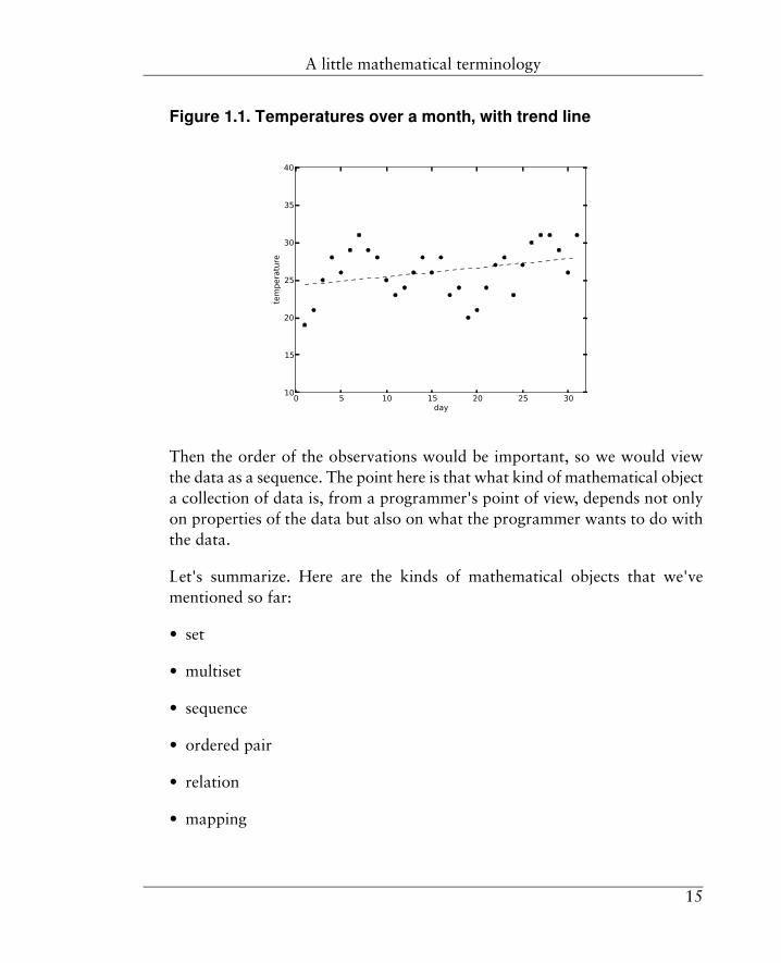
Figure 1.1. Temperatures over a month, with trend line

Then the order of the observations would be important, so we would viewthe data as a sequence. The point here is that what kind of mathematical objecta collection of data is, from a programmer's point of view, depends not onlyon properties of the data but also on what the programmer wants to do withthe data.

Let's summarize. Here are the kinds of mathematical objects that we'vementioned so far:

• set

• multiset

• sequence

• ordered pair

• relation

• mapping

15


And here are the instances of these mathematical objects that we've observedin our examples:

• A generic file: a sequence of sequences.

• The data for our first script (names, Example 1.1): a set.

• The data for our second script (emails, Example 1.2): a set of ordered pairs,forming a relation, possibly a mapping.

• The data for our third script (average of observations, Example 1.3): amultiset. But if we want to use the same data to plot a trend, a sequence.

In later chapters we'll explore properties of these and other mathematicalobjects and their connections with the data and computations of programs.Meanwhile, let's conclude the chapter with two simple observations:

• A collection of data, as a programmer views it, is likely to be a set, or asequence, or a mapping, or some other well-known mathematical object.

• You can often view a collection of data as more than one kind ofmathematical object, depending on what you want to do with the data.

Terms introduced in this chaptermappingscriptassociative propertysetcommutative propertysequencemultisetordered pair

relation

16

Terms introduced in this chapter

Chapter 2An overview of Python2.1. Introduction

In this chapter and the two chapters that follow we'll give an overview of thePython language, enough (we hope) for you to understand the Python examplesin the rest of the book. Along the way, we'll introduce terms for many Pythonconcepts. Most of these terms are not specific to Python, but are part of thecommon language for speaking about programming languages in the computerscience community. We'll use these terms in many places later in the book;so, even if you already know Python, you might want to skim through thechapters just to make sure that you are familiar with all the terms.

You have seen examples of Python programs that take their input data fromfiles. In fact, Python programs themselves are made of text in files. If you hadthe scripts of the previous chapter on your computer, each would be in a fileof its own.

On most computer systems, you can also use the Python interpreterinteractively. You can type small bits of Python to the interpreter, and it willdisplay the results. For example, you can use the interpreter as a calculator.You can type

3 + 2

and the interpreter will display

5

If you have your computer handy as you are reading this book, you mightlike to experiment with the Python constructs that you are reading about. Goahead and type pieces of Python to the interpreter and see what happens. Feelfree to do this at any time as you read.

17

2.2. Values, types, and namesWe'll start by explaining some very basic concepts of Python; you might thinkof these as defining how to think about computation in the Python world.

Computation in Python is done with values. Computations operate on valuesand produce other values as results. When you type “3 + 2” to the Pythoninterpreter, Python takes the values 3 and 2, performs the operation of additionon them, and produces the value 5 as a result.

We have seen a few kinds of values already. The numbers 3 and 2 are values.So are sequences of characters like “John”. So are more complicated thingslike the opened files that the scripts of Chapter 1 used. As we'll see in laterchapters, Python values also include other kinds of sequences, as well as setsand mappings and many other kinds of things.

Every value has a type. The type of whole numbers like 3 and 2 is “integer”.The type of a sequence of characters is “string”. There are other types inPython, and we'll see many of them later in the book.

A type is more than just a Python technical term for a kind of value. A typehas two important properties, besides its name: a set of possible values, andthe set of operations that you can do with those values. In Python, one of theoperations on integers is addition, and one of the operations on strings issplitting at a given character.

Finally, names are central to Python programming, and they are used in manyways. One important example is this: we can bind a name to a value. That'swhat happened when we did this in our script that computed an average:

count = 0

This binds the name count to the value 0. Another name for the operation inthis example is assignment: we say that we assign 0 to count and if a line likethis occurs in a Python program, the line is called an assignment statement.There are several ways to bind a name to a value in Python, but the assignmentstatement is the most basic way.

18

Values, types, and names

A name that is bound in an assignment statement like this is called a variable.That's because the binding is not necessarily permanent: the name can bebound to a different value later. For example, our script for computing anaverage has this line farther along:

count += 1

This binds count to a new value, which is one greater than the value that itwas bound to before. A program can do such rebinding many times, and infact our averaging script does: once for each line of the file of observations.

In Python you could even do this in the same program, although you probablywouldn't want to:

count = "Hello, John!"

So even the type of a variable isn't permanent. In Python, a type is a propertyof a value. We can speak of the type of a variable, but that's just the type ofthe value that happens to be bound to that variable.

However, as Python is actually used in practice, most variables have the sametype throughout a program — that just turns out to be the most natural wayfor programmers to use variables. Furthermore, good programmers choosenames that have some logical relationship with the way that the names areused. Giving a name like count to a string like "Hello, John!" is just silly,even though the Python interpreter would let you do it.

Saying that an assignment binds a name to a value is actually a slightoversimplification in Python. What actually happens is that a name is boundto something called an “object”, and it's the object that has a value. Later inthe book we'll see how the distinction can make a difference. For now, thisfine point isn't important, and we can just think of the name as being bounddirectly to the value.

2.3. IntegersPython integers are like mathematical integers: that is, they are the positiveand negative whole numbers and zero.

19

Integers

Some of the operations that you can do with integers in Python, as you mightexpect, are addition, subtraction, multiplication, and division. Each of theseoperations is denoted by a symbol that comes between the quantities operatedon, like this:

3 + 23 - 23 * 23 / 2

Each of those symbols is called an operator, and the quantities that theyoperate on are called operands. Many operators, like these, operate on twooperands; such operators are called binary operators. (The term “binary”,when used in this way, doesn't have anything to do with the binary numbersystem.)

In a Python program, a sequence of one or more digits, like 123 or 2 or 0,represents a non-negative integer value. The sequence of digits is an exampleof a constant: a symbol that can't be bound to anything other than the valuethat it represents.

To get a negative integer, we precede a sequence of digits with a minus signin the obvious way, like this:

-123

Here, the minus sign is a unary operator, meaning that it takes only oneoperand. Notice that - can be either a binary operator or a unary operator,depending on context.

The combination of an operator and its operands is called an expression. Asin most programming languages, larger expressions can be built up bycombining smaller expressions with operators, and parentheses can be usedfor grouping. We speak of evaluating an expression: this means finding thevalues of all its parts and performing all the operations to obtain a value.

If the operands of the +, -, and * operators are integers, the result is also aninteger. The operator / is different: for example, the result of evaluating theexpression 3 / 2 is 1.5 just as in mathematics. But that 1.5 is not an integer,

20

Integers

of course, because it has a fractional part. It's an example of a floating-pointnumber; we'll explain numbers of that type in the next section.

In Python, the result of dividing two integers with the / operator is always afloating-point number, whether the division comes out even or not. There'sanother division operator that always gives an integer result: it is //. So, forexample, the value of 4 / 2 is the floating-point number 2.0, but the value of4 // 2 is 2, an integer. If the result of // does not come out even, it is roundeddown, so that the value of 14 // 3 is the integer 4, with no fractional part;the remainder, 2, is dropped.

The operator % gives the remainder that would be left after a division. Thevalue of 14 % 3 is 2, for example.

Python has other integer operators. Here's one more: ** is the exponentiationoperator. For example, 2 ** 8 means 28.

Python also has operators that combine arithmetic and assignment: these arecalled augmented assignment operators. We have already seen one of these,the += operator, in this augmented-assignment statement:

count += 1

In evaluating this statement, the Python interpreter does the + operation inthe usual way and then binds the left operand to the result. Python also has-= and *= and so on, but the += operator is probably the one that programmersuse most often.

In Python, there is no intrinsic limit on the size of an integer. The result ofevaluating the expression 2**2**8 is a rather large number, but it's a perfectlygood integer in Python, and Python integers can be much larger than that one.

However, there are practical limits to the size of a Python integer. You can'tevaluate the expression 2**2**100 using the Python interpreter. That valuewould contain far more digits than your computer can store, and even if thePython interpreter could find somewhere to put all the digits, evaluating theexpression would take an enormously long time.

21

Integers

In mathematics, 22100is a perfectly good number. It's a finite number, and it

isn't hard to denote finite numbers that are much larger than that one: thinkof raising 2 to that power, for example. In mathematics there are also waysof making sense of infinite numbers, and mathematics draws a distinctionbetween all finite numbers and the infinite numbers.1

Unlike many programming languages, Python has a way of representing“infinity”, as we'll see in the next section. There is only one infinite number(and its negative) in Python, and the Python “infinity” has rather limitedusefulness in Python programs, but it does exist.

In Python programming, and in all programming for that matter, it's importantto recognize a third category of numbers, besides finite and infinite: numbersthat are finite but that are far too large to compute with in practice, such as22100

.

As we'll see in later chapters, sets can be represented as Python values, andso can sequences, mappings, and other mathematical structures. As withintegers, the Python values are similar to the mathematical objects; Pythonwas designed so that they would be. That's good, because we can usemathematical thinking to describe and understand those values and theoperations on them. But, as with integers, Python sets and sequences and therest have practical limitations. For example, a Python programmer must avoidcomputations that would try to construct sets that are far too large to storeor operate on.

So, whereas in mathematics there's a distinction between finite and infinite,in programming there's also a distinction between finite and finite-but-far-too-large. The distinction applies to computations too: there are manycomputational problems that can't be solved in practice because thecomputations would take far too long. Drawing a line between practical andimpractical, and categorizing values and computations according to whichside of the line they are on, are central issues in the field of computer science,as you will see later in your studies if you are a computer science student.

1Yes, in mathematics there are different infinite numbers. For example, the number of points on a lineis greater than the number of integers: infinitely greater, in fact.

22

Integers

2.4. Floating-point numbersIn Python, the floating-point numbers are another type, whose name is "float".Python uses floating-point numbers to represent numbers with a fractionalpart, and produces them in computations that may not come out even, likedivision of two integers using the / operator. As Python integers representmathematical integers, Python floating-point numbers represent the realnumbers of mathematics. Floating-point numbers are only an approximaterepresentation of the real numbers, though; they differ from mathematicalreal numbers in some important ways, as we will see.

Python has two kinds of floating-point constants. The first is simply a sequenceof digits with a decimal point somewhere in it; 3.14 and .001 are examples.The second is a version of “scientific notation”: the number 6.02 × 1023 canbe written in Python as 6.02E23. The number after the “E” (you can also use“e”) is the power (“exponent”) of ten used in the scientific notation; it canbe negative, as in 1e-6, which represents one millionth.

Floating-point arithmetic in Python is much like integer arithmetic, exceptthat if the operands in an expression are floating-point, so is the result.Floating-points and integers can be mixed in an expression: if one operand ofa binary operator is a floating-point and the other is an integer, the integer isconverted to a floating-point value and then the operation is done, giving afloating-point value.

To convert explicitly from an integer to a floating-point number or vice versa,we can use a Python function. As we'll see in later chapters, Python functionscan behave in several different ways, but the kind that we'll consider now islike a mathematical function. It's a mapping: it takes a value, called anargument, and produces another value as a function of the argument.

To use a function, we write a function call, which is another kind of expressionbesides those that we have seen. In the form that we'll consider now, a functioncall consists of the name of a function, followed by an expression inparentheses; that expression is the argument. When the Python interpreterevaluates a function call, we say that it calls the function, passing the argument

23

Floating-point numbers

to the function. The function returns a value, which becomes the value of thefunction call expression.

To convert an integer value to floating-point, we can use the float function.For example, if the variable n has the value 3, then float(n) has 3.0 as a value.To convert from floating-point to integer, we can use the int function if wejust want to truncate the fractional part, or the round function if we want toround to the nearest integer. For example, if the variable x has the value 2.7,the value of int(x) is 2 and the value of round(x) is 3.

We can also use float to create a Python representation of “infinity”. Pythonhas no constant that represents “infinity”, but we can create the Python valuethat represents “infinity” by writing float("inf") or float("Infinity") (thestring passed to float can have any combination of upper-case and lower-caseletters). We can get the negative infinity by writing float("-inf") or-float("Infinity") or similar expressions.

Probably the most useful property of the Python “infinity” is that it is afloating-point number that is greater than any other floating-point numberand greater than any integer. Similarly, the Python “negative infinity” is afloating-point number that is less than any other floating-point number andless than any integer. Except for showing a few applications of those properties,we won't say much more about Python's positive and negative infinity in thisbook.

Floating-point numbers (except for positive and negative infinity) are storedin the computer using a representation that is much like scientific notation:with a sign, an exponent, and some number of significant digits. On mostcomputers, Python uses the “double precision” representation provided bythe hardware.

For our purposes here, the exact representation isn't important, except forone point: both the exponent and the significant digits are represented usinga fixed number of bits. An interesting consequence of this is that only finitelymany floating-point numbers are representable on any given computer. Infact, in Python there are many more integers than floating-point numbers!This is the opposite of the situation in mathematics.

24

Floating-point numbers

Notice that there must be a limit to the magnitude of a floating-point number,since there's an upper bound to the value of the exponent. This limitationusually isn't serious in practice, though, since on modern computers a floating-point number can easily be large enough for almost all common uses, such asrepresenting measurements in the physical universe.

A more important limitation is that a floating-point number contains only alimited number of significant digits. This means that most of the mathematicalreal numbers can be represented only approximately with floating-pointnumbers. It also means that the result of any computation that produces afloating-point result, such as evaluating the expression 1/3, will be truncatedor rounded to a fixed number of significant digits, giving only anapproximation to the true mathematical value in most cases.

Thus, we must be careful when we compute with floating-point numbers,keeping in mind that they are only approximations. For example, we can'tassume that the value of 1/3 + 1/3 + 1/3 is exactly equal to 1.0; we can onlyassume that the two values are approximately equal. The difference betweena floating-point result and the true mathematical value is called roundoff error;in some situations, especially in long computations, roundoff error can buildup and cause computations to be unacceptably inaccurate.

2.5. StringsAs we have already mentioned, sequences of characters are called strings. InPython, a string can contain not only the characters available on yourkeyboard, but all the characters of the character set called “Unicode”. Unicodecontains characters from most of the world's written languages, includingChinese, Arabic, Hindi, and Cherokee, to name just a few. Unicode alsocontains mathematical symbols, technical symbols, unusual punctuation marks,and many more characters. For our purposes in this book, though, thecharacters on your keyboard will be enough.

A string constant is any sequence of characters enclosed in double-quotecharacters, as in

"Here's one"

25

Strings

or single-quote characters, as in

'His name is "John"'

Notice how a string delimited by double-quote characters can contain single-quote characters and vice versa.

The sequence of characters in a string may be empty, as in ""; this string iscalled the empty string or the “null string”. Yes, the empty string does haveuses, as we will see.

Python has no “character” type; it treats a single character as the same as aone-character string.

There is a function to convert from other types, such as integers and floating-point numbers, to strings: its name is str. For example, str(3) produces thestring value "3".

One important operation on strings is concatenation, meaning joining togetherend-to-end. Python uses the + operator for concatenation. For example, thevalue of the expression "python" + "interpreter" is

"pythoninterpreter"

So Python gives the + operator three different meanings that we've seen sofar: integer addition, floating-point addition, and string concatenation. Wesay that + is overloaded with these three meanings.

Python also overloads * to give it a meaning when one operand is a string andthe other is an integer: this means concatenating together a number of copies.For example, the value of 3 * "Hello" is "HelloHelloHello". The integer canbe either the left or the right operand. But Python doesn't overload + or * forany imaginable combination of types. For example, Python doesn't allow +

of a string and an integer. You might guess that the Python interpreter wouldconvert the integer to a string and do concatenation, but it won't.

26

Strings

Terms introduced in this chapterevaluatingtypefloating-pointnameaugmented assignmentbindingfunctionassignmentargumentassignment statementfunction callvariablecalling a functionintegerpassing an argumentoperatorreturnoperandempty stringbinary operatorconcatenationconstantoverloadingunary operator

expression

Exercises1. We said that 228

was a perfectly good Python value but that 22100was far

too large. For expressions of the form 2**2**n, what values of n make thevalue of the expression too large to compute in practice? Experiment withyour Python interpreter. Start with small values of n and then try largervalues. What happens?

2. What happens if you actually try to evaluate 2**2**100 using your Pythoninterpreter? Let it run for a long time, if necessary. Can you explain whatyou see?

3. Estimate how many decimal digits it would take to write out 22100. Hint:

logarithms. You can use your computer, if that will help.

4. The value of a comparison like 1.0 == 1 is either True or False. Experimentwith your Python interpreter: you will probably get True for the value of1.0 == 1, for example. Try 1/3 + 1/3 + 1/3 == 1.0; you may get True orFalse, depending on how the rounding is done on your computer. Try to

27


find some comparisons that should give True according to mathematicalreal-number arithmetic, but that give you False in Python on your computer.

5. Does concatenation of strings have the associative property, as addition ofintegers does? Does concatenation of strings have the commutative property?

6. Make an improvement to the script that reads a file and finds lines thatbegin with “John”. Change it so that it actually compares the first nameon each line with the name “John”, so that (for example) it doesn't displaylines starting with “Johnson”. You have already seen enough of Pythonthat you should be able to guess how to do this. Assume that each line ofthe file contains just a first name, a single blank space, and a last name.Test your solution using the Python interpreter.

28

Exercises

Chapter 3Python programs3.1. Statements

Now we'll take the concepts and Python constructs from the last chapter andsee how they can be used in larger Python constructs, up to and includingwhole programs.

A Python program is a sequence of statements. To illustrate some of the kindsof Python statements, let's look again at one of the sample programs fromSection 1.2.

sum = 0count = 0



print(sum/count)

This program contains several statements. Some of them are assignment andaugmented-assignment statements; each is on a line of its own.

If a statement is too long to fit on one line, it can be broken across lines byusing the backslash character \ followed by a line break, like this:

z = x**4 + 4 * x**3 * y + 6 * x**2 * y**2 \+ 4 * x * y**3 + y**4

However, if the line break is inside bracketing characters such as parentheses,the backslash is not needed:

z = round(x**4 + 4 * x**3 * y + 6 * x**2 * y**2+ 4 * x * y**3 + y**4)

29

The last line of the sample program is also a statement. As it happens, printis a function in Python. (Here, its argument is a floating-point number, butin the examples of Section 1.2 we also saw print being used to display strings.In fact, print is overloaded to work with these and many other Python types.)

An expression in Python, by itself, can be a statement, and the last line of theprogram is an example. For the expressions that we have considered untilnow, using one as a statement would make no sense; the Python interpreterwould just evaluate it and do nothing with the result. But some expressionshave side effects: evaluating them has some effect besides producing a value.

Some Python functions are designed to be used as statements. They aren'tmappings at all, because they don't produce values; they only cause side effects.The print function is one of these. Its “side effect”, which is really its onlyeffect, is to display a value.

Assignment statements, augmented assignment statements, and expressionstatements are called simple statements. The line starting with “for” and thethree lines that follow it are an example of a compound statement: a statementwith other statements inside it.

for line in file:n = int(line)sum += ncount += 1

The first line of a compound statement is called its header. A header startswith a keyword that indicates what kind of compound statement it is, andends with a colon. Python has a number of keywords that are used for specialpurposes like this. As it happens, both for and in are keywords; they arestructural parts of the header. Keywords can't be used as names; you can'thave a variable named “for” or “in”.

The remaining lines of a compound statement, called the body of the statement,are indented with respect to the header.

As we have already seen, programs can contain blank lines, which are notstatements and have no effect on what the program does, but are strictly for

30

Statements

the benefit of human readers. Similarly, all serious programming languagesprovide for comments, so that a programmer can insert commentary andexplanations into a program. In Python, a comment starts with the character“#” and continues to the end of the line. Here's the average-of-numbers scriptagain with some comments added:

# A program to display the average of# the numbers in the file "observations".# We assume that the file contains# whole numbers, one per line.

sum = 0count = 0


n = int(line) # convert digits to an integersum += ncount += 1

print(sum/count)

3.2. ConditionalsIn a sequence of statements, the Python interpreter normally executes thestatements one after another in the order they appear. We say that the flowof control passes from one statement to the next in order.

Sometimes the flow of control needs to be different. For example, we oftenwant certain statements to be executed only under certain conditions. Aconstruct that causes this to happen is called a conditional.

The basic conditional construct in Python is a compound statement that startswith the keyword if. We call such a statement an if-statement for short. Themost basic kind of if-statement has this form:

if condition :

statements

Here's an example that we saw in Section 1.2:

31

Conditionals

if name == "John Davis":print(email)

Most commonly, the condition in an if-statement header is a comparison, asin the example above. The result of a comparison is a value of the Booleantype. This type has only two values, True and False, and that's the wayconstants of the Boolean type are written. These values behave like the integers1 and 0 in most contexts — in fact, Python considers them numeric valuesand you can do arithmetic with them — but the main use of Boolean valuesin Python is to control execution in if-statements (and in the while-statementsthat we'll see in the next section).

The comparison operator that means “does not equal”, like “≠” inmathematics, is written != in Python. The operators < and > mean “is lessthan” and “is greater than”, as you might expect. For “is less than or equalto”, like “≤” in mathematics, Python uses <=, and similarly >= means “≥”.

One more comparison operator is in, which (for example) can be used to testwhether a character is in a string. Here is an example, where c is a variablecontaining a character:

if c in "aeiou":print("c is a vowel")

More generally, if the operands of in are strings, the operator tests whetherthe left operand is a substring of the right operand; in other words, whetherthe sequence of characters of the left operand occurs as a sequence of charactersin the right operand. We'll see many more uses for the in operator in laterchapters.

Python has operators whose operands are Booleans, too: and, or, and not.The not operator is unary, and produces False if the value of its operand isTrue and True if the value of its operand is False, as you might expect.

The or operator also means what it appears to mean, but Python evaluates itin a particular way. In evaluating an expression of the form A or B, the Pythoninterpreter first evaluates A. If its value is True, the value of the wholeexpression is True; otherwise, the interpreter evaluates B and uses its value as

32

Conditionals

the value of the whole expression. The and operator is evaluated similarly: theinterpreter evaluates the second operand only if the value of the first is False.

So, for the or and and operators, the interpreter doesn't just evaluate bothoperands and then do the operation, as it does with most operators. This canmake a difference. Look at this example:

if y != 0 and x/y > 1:

If y is zero, the value of the whole Boolean expression is False, and the Pythoninterpreter doesn't even evaluate x/y > 1. That's fortunate in this case, becausedividing by zero is undefined in Python just as it is in ordinary arithmetic.

Python if-statements can have other forms, to create other kinds of controlflow that occur commonly in programs. For example, often a program needsto do one thing if a condition is true and something else if the condition isfalse. The Python statement that does so has this form:

if condition :

statementselse:

statements

This is a compound statement with more than one “clause”, each with itsown header and body; the headers are aligned with each other. Here's a simpleexample:

if a > b:print("I'll take a")

else:print("I'll take b")

To distinguish more than two cases and handle them differently, you cancombine if-statements, as in this example:

33

Conditionals

if testScore > medianScore:print("Above average."

else:if testScore == medianScore:

print("Average.")else:

print("Below average.")

Here we have one if-statement that contains another if-statement. By definition,a compound statement contains other statements, and these can be compoundstatements themselves.

When constructs contain other constructs of the same kind, we say that theyare nested. Expressions are another example since, in an expression thatcontains an operator, the operands can be expressions themselves. Nestedconstructs appear in many places in programming languages.

The pattern of control flow in the above example is so common that Pythonprovides a shorter way to do it. An if-statement can contain a clause beginningwith elif, meaning “else if”, between the if-clause and the else-clause:

if condition :

statementselif condition :

statementselse:

statements

So the example above could be written more concisely like this:

if testScore > medianScore:print("above average."

elif testScore == medianScore:print("average.")

else:print("below average.")

There can be more than one elif-clause, for computations in which there aremore than three cases. The else-clause can be omitted whether or not thereare elif-clauses. Thus, the general form of the if-statement in Python is an if-

34

Conditionals

clause, followed optionally by one or more elif-clauses, followed optionallyby an else-clause.

3.3. IterationsAnother pattern of control flow is extremely common in programs: executingthe same section of code many times. We call this iteration.

Some iterations execute a section of code over and over forever, or at leastuntil the program is interrupted or the computer is shut down. But we'llconcentrate on the kind of iteration that executes a section of code as manytimes as necessary, according to the circumstances, and then stops.

Here's an example that we've already seen (Example 1.1):

file = open("names")for line in file:


The compound statement starting with the keyword for is a Python iterationconstruct, the for-statement. As we have seen, this for-statement repeats itsbody as many times as there are lines in file. Since we're emphasizingmathematical structures throughout this book, iterations like this one — thosethat iterate over all elements of a sequence or set or other mathematicalstructure — will be especially important to us.

The general form of a for-statement is this:

for name in expression :

statements

The expression provides the values to be iterated over. To give a simpleexample, the expression's value can be a string, which is a sequence ofcharacters, as in the following:

35

Iterations

sentence = "Look at me swimming!"

vowels = 0for c in sentence:

if c in "aeiou":vowels += 1

print("There are " + str(vowels)+ " vowels in that sentence.")

One way or another, the expression in the header must provide a sequence ofvalues. For each of those values, the Python interpreter binds the name in theheader to the value and then executes the body of the for-statement.

Python for-statements can iterate over many kinds of things. Some of themare composite values that exist in advance, like strings. Others are sequencesof values that are generated dynamically, one at a time, by objects callediterators. For example, look at this little program again:



Here's what really happens: the value that the function open returns is aniterator. The for-statement uses the iterator to generate values: on eachrepetition, the iterator reads a line of the file and returns it to the for-statement,which binds that string to line and executes the body of the for-statement.

A “range” object is another kind of value that is useful in iterations. For aninteger value n, a function call range(n) produces a range object that generatesthe sequence of integers from 0 to n-1, much as an iterator does, withouthaving to create the entire sequence in advance. The most common use ofrange is in the header of a for-statement, like this:

for i in range(n):

This causes the body of the for-statement to be executed n times, with i takingon successive values from 0 to n-1, acting as a counter. Here's a simple examplethat displays the powers of 2 from 0 to 19:

36

Iterations

for i in range(20):print("2 to the " + str(i)

+ " power is " + str(2**i))

We'll see many more examples of for-statements in later chapters. Especially,in the chapters that discuss mathematical structures in more detail, we'll seemany examples of for-statements that iterate over elements of those structures.

Python has one more kind of compound statement for doing iteration: thewhile-statement. Its form is as follows:

while condition :

statements

Its meaning is this: the body of the while-statement is executed over and overuntil the condition in the header becomes false. Specifically, to execute a while-statement, the Python interpreter first evaluates the condition. If it is false,control passes immediately to whatever follows the while-statement. Otherwise,the interpreter executes the body and then evaluates the condition again, andso on.

In some ways the while-statement is more basic than the for-statement: anyiteration that can be done with a for-statement can be done with a while-statement, although not always as easily. Look at this example again:

for i in range(20):print("2 to the " + str(i)

+ " power is " + str(2**1))

Here's how we can do the same computation using a while-statement:

i = 0while i < 20:

print("2 to the " + str(i)+ " power is " + str(2**1))

i += 1

In the for-statement version, the iteration mechanism is all on one line. In thewhile-statement version, we need three lines: one to initialize the counter i tozero, one to increment the counter, and one (the while-statement header) totest the counter to determine when the iteration is done.

37

Iterations

Here's another situation in which some programmers would use a while-stament: reading all lines of a file. Python has a function readline for readingone line of a file at a time. Actually, readline is a particular kind of a functioncalled a “method”, which we'll discuss later; for now, let's just say thatreadline can be used like this:

line = file.readline()

Each time this statement is executed, line is assigned the next line in file, asa string. When there are no more lines in the file, line is assigned the emptystring.

So, to do some computation on every line of a file, we can use a pattern ofcode like this:

line = file.readline()while line != "":

computation using lineline = file.readline()

Again, we have an initialization step, the first call to readline; a test; and astep that advances the iteration for the next repetition of the computation,the second call to readline. But, as we have seen, we can do the job moreeasily with a for-statement:

for line in file:computation using line

So it's usually easier to use a for-statement than a while-statement, wheneverthe for-statement is an obvious fit for the computation that needs to be done;that is, whenever you can identify an obvious sequence or other collection ofvalues to iterate over. But for some computations there really isn't any.

Here's an example. This piece of program calculates the square root of anumber using an algorithm called “Newton's Method”. We assume that thenumber is in the variable n and that it is non-negative; we will calculate a closeapproximation to its positive square root and leave that approximation in thevariable root. (The function abs gives the absolute value of an integer or afloating-point number.)

38

Iterations

guess = 1.0while abs(n - guess*guess) > .0001:

guess = guess - (guess*guess - n)/(2*guess)root = guess

If you have studied calculus, you might be able to see how Newton's Methodworks here and why guess*guess gets closer and closer to n so that the iterationeventually terminates. In any case, notice that there's no sequence here, otherthan the sequences of values that the variable guess gets on successiveexecutions of the while-statement body.

Terms introduced in this chapterconditionalstatementif-statementside effectBooleansimple statementsubstringcompound statementnestingheaderiterationbodyfor-statementkeyworditeratorcommentwhile-statementflow of control

Exercises1. Write a program that will display a bar chart based on data from a file.

The file is called “data”, and it contains non-negative integers, one per line.

The output of your program should look like the following (for a filecontaining 7, 15 and 11, as an example):

####### 7############### 15########### 11

2. Take your solution to the previous exercise and modify it so that it imposesa maximum length of the bars. If an integer from the file is greater than

39


25, your program will display only a bar of length 25. Here's how a barchart might look now (with different data):

####### 7######################### 25######################### 283########### 11

3. Now take your solution to the previous exercise and modify it again. If aninteger from the file is greater than 25, your program will display a bar oflength 25, but with an ellipsis ("/ /") in the middle, like this:

####### 7######################### 25###########/ /########### 283########### 11

4. Experiment with the square-root program of Section 3.3. Put a print

expression-statement in the body of the while-statement to display the valueof guess, and see how long it takes the iteration to converge for differentvalues of n and different initial guesses. What happens if n is a negativenumber?

5. The first line of our square-root program is this:

guess = 1.0

What happens if you change it to this?

guess = 1

Try it, and explain what you see.

6. If you have studied calculus, try to explain how the square-root programworks. (Hint: we are solving for x in the equation x2 = n; that is, x2 - n =0, where n is a constant. The derivative of x2 - n is 2x. Draw a picture.)

40

Exercises

Chapter 4Python functions4.1. Function definitions

In this chapter we'll see how to define functions in Python and see some ofthe many things we can do with functions.

As we have seen, some Python functions compute values and some produceside effects. The latter kind are called “subroutines” or “procedures” in someprogramming languages, but in Python both kinds are called “functions” andare defined in the same way.

Here's an example of a function definition. As we have seen, Python alreadyhas an absolute-value function, but if it didn't we could define our own likethis:

def abs(n):if n >= 0:

return nelse:

return -n

A function definition is a compound statement. Its header contains the functionname and the name of the function's parameter. When the statement isexecuted, Python binds the function name to the code in the statement's body,as well as to other details such as the name of the parameter. The body is notexecuted yet. When the the function is called, the parameter name is boundto the value of the argument that is passed to the function, and the body isexecuted. A return-statement, a statement containing return and possibly anexpression, terminates the execution of the function body. It also causes thevalue of the expression, if there is one, to be returned from the function, andthis value becomes the value of the function-call expression.

Notice that the type of the parameter is not declared anywhere. In fact, theargument passed to this function can be any value for which the operations

41

“>=” and unary “-” are defined. Thus, the function is automatically overloadedfor integer and floating-point arguments; we don't need to do anything specialto make that happen.

As another example, here's how we could take the square-root computationfrom the previous chapter and package it as a function:

def sqrt(n):guess = 1.0while abs(n - guess*guess) > .0001:

guess = guess - (guess*guess - n)/(2*guess)return guess

Until now, all the functions that we have seen have had exactly one parameter,but a function can have more than one. For example, the iteration in thefunction above terminates when guess is close to the true square root of n.The stopping criterion is that the square of guess equals n to within a toleranceof .0001, but we could define the function so that the tolerance is anotherparameter, like this:

def sqrt2(n,tolerance):guess = 1.0while abs(n - guess*guess) > tolerance:

guess = guess - (guess*guess - n)/(2*guess)return guess

Then we would call sqrt2 with two arguments. For example, the callsqrt2(3,.00005) would do the computation using .00005 as the tolerance.

By the way, we saw another syntax for function calls in the examples ofChapter 1 and Section 3.3:

line.startswith("John")line.split(",")line = file.readline()

This is the syntax that Python uses for calls to a particular kind of function,called a “method”, which we will see in Chapter 11. For now, it's enough tosay that the value before the “.” is used as the first argument in the functioncall, and any remaining arguments are enclosed in parentheses after thefunction name as usual.

42

Function definitions

Now what about functions that don't return values? One typical use for themis to produce output, perhaps as the result of a computation. For example,consider the script from Chapter 1 that calculates and prints the average ofnumbers in a file (Example 1.3). That script could be made into a function,perhaps like this:

def printAverageOfFile(fileName):sum = 0count = 0

file = open(fileName)for line in file:


print("Average of numbers in " + fileName + ":")print(sum/count)

Here, the name of the file is a parameter of the function. This design lets useasily perform the same computation on more than one file, like this:

printAverageOfFile("observations-April")printAverageOfFile("observations-May")printAverageOfFile("observations-June")

It is possible to define a Python function that produces side effects and thenreturns a value as well. However, many programming experts believe that aprogram's design is cleaner if every function has only one purpose, and eitherreturns a value or causes side effects but not both. We'll usually stick to thatprinciple in this book.

4.2. Recursive functionsAs in most modern programming languages, a function definition in Pythoncan be recursive, meaning that the function body can call the same functionthat is being defined. In other words, the function is defined at least partiallyin terms of itself.

The classic example is the factorial function. For a positive integer n, thefactorial of n, written n!, can be defined mathematically this way:

43

Recursive functions

n! = n · (n-1) · … · 2 · 1

This recursive definition has a different structure but has the same effect:

n! = 1 if n = 1n! = n · (n-1)! otherwise

Here is the corresponding Python function definition:

def factorial(n):if n == 1:

return 1else:

return n * factorial(n-1)

Then suppose factorial is called, say with an argument of 5. Notice howfactorial will keep calling itself, first with an argument of 4, then 3, then 2,and finally 1. At that point factorial will immediately return 1. Then all therecursive calls to factorial will return their results in reverse order:factorial(2) returning 2*1 = 2, factorial(3) returning 3*2 = 6, factorial(4)returning 4*6 = 24, and finally factorial(5) returning 5*24 = 120.

A good recursive function definition has the following characteristics:

• It is defined by cases (in Python, usually with an if-statement). At least oneof the cases is not recursive: it defines the result directly, rather than in termsof a recursive reference to the function being defined. Such a case is calleda basis case. In the factorial example, there is one basis case, the case inwhich n = 1.

• Every sequence of recursive calls eventually leads to a call in which one ofthe basis cases applies. Usually, the basis cases treat the situations in whichthe argument is “small” or “simple” or “trivial” in some sense, and therecursive cases (the cases that are not basis cases) take the function'sparameter and recursively call the function with an argument that is“smaller” or “simpler” or closer to the basis case in some way. In thefactorial example, the recursive case takes the parameter n and recursivelycalls the function with the argument n-1. It is easy to see that every sequence

44

Recursive functions

of recursive calls will eventually end with n = 1, assuming that n is a positiveinteger in the original call.

We won't give a comprehensive treatment of recursive programming in thisbook, but we will see recursive functions again several times. In any case,recursion can be a useful and powerful programming technique and you willprobably have many occasions to use it throughout your programming career.

4.3. Functions as valuesIn Python, functions are values, much as integers and strings are. A function-definition statement binds a name to the function's definition, and in Pythonthis works very much like binding a name to a value in an assignmentstatement. Let's explore some of the implications of these facts.

First, once we have defined a function, we can bind another name to thatfunction. One way to do this is with an assignment statement, as in thisexample:

def square(x):return x*x

sq = square

Now sq is bound to the same function definition that square is, so it computesthe same thing. For example, the value of sq(3) would be 9.

We can also pass a function as an argument to another function. Here's anexample: the function below takes as parameters a function and another value,and returns the result of applying the function to the argument twice.

def twice(f,a):return f(f(a))

So, for example, consider the function call twice(square,3), where square isas defined above. The Python interpreter binds f to the function square anda to 3, and so returns square(square(3)), which is 3 to the fourth power, or81. Similarly, the value of twice(sqrt,3) is the fourth root of 3.

45

Functions as values

Here's a somewhat more useful example. We can define a Python functionthat will compute an approximation to the derivative of a function at a givenpoint. (For readers who haven't studied calculus: the derivative of a functionis the rate of change of the function's value. Consider a function of oneargument, f(x). Picture a plot of f(x) in the vertical direction against x in thehorizontal direction. The derivative of the function at a given value of x is theslope of the curve at that value of x.)

The function below does the job. It takes a function f, a value x, and a smallvalue dx to be used as the magnitude of a small interval. Then the functionderivAt returns the change in value of f over an interval of length dx, startingat x, divided by the length of the interval, giving an approximation to themathematical derivative of f at x.

def derivAt(f,x,dx):return (f(x+dx) - f(x))/dx

Mathematically, the derivative of x2 is 2x, so the exact value of the derivativeof the square function at the point 3 should be 6. Using the definition ofderivAt above, derivAt(square,3,.00001) should give us an approximationto that value, and in fact Python does give us a value close to 6.

In Python a function can even return another function as a value. A functioncan execute a function-definition statement, creating a new function andbinding that function to a name, and then return the value bound to thatname. Here's an example. The function multiplyBy takes a number as aparameter and returns a function that multiplies by that number.

46

Functions as values

def multiplyBy(n):def times(m):

return m*nreturn times

Remember, a function definition is an executable statement. Here the definitionof times is executed when the body of multiplyBy is executed. The value thatis used for n in the new function is the value that is bound to n at that time,which is the value of the argument that is passed to multiplyBy. Since m is aparameter of the new function, it is not bound until that function is called.

We can use multiplyBy like this:

double = multiplyBy(2)triple = multiplyBy(3)

Then when we evaluate double(7), m is bound to 7, the multiplication is done,and we get 14. Similarly, the value of triple(33) is 99.

The programming technique that we just used is a special case of a moregeneral technique: to bind some but not all arguments of a function, leavingit a function of fewer arguments. This is called partial application. Here's afunction that binds the first argument of any two-argument function, leavingit a function of one argument.

def partial(f,x):def f_x(y):

return f(x,y)return f_x

The function partial takes a two-argument function f(x,y) and a value for x,and returns a one-argument function that we can denote as fx(y): it is f(x,y)with the value of x held constant, and there is a different such function foreach different value of x. For example, if mult is a function of two argumentsthat returns their product, the value of partial(mult,2) is the same functionas multiplyBy(2).

As a final example, let's define a function that will take the derivative ofanother function. It doesn't take the derivative symbolically, as in calculus,

47

Functions as values

but it returns a function that gives an approximation to the derivative at anygiven point. Here's how we can write it.

def deriv(f,dx):def d(x):

return derivAt(f,x,dx)return d

We call deriv with a function of one argument, say square, and a number touse as an interval size. The new function d uses those values for f and dx inits call to derivAt, but the new function is still a function of one argument,x. We can use deriv like this:

derivOfSquare = deriv(square, .00001)

Then the value of derivOfSquare(3) is a number close to 6, just as we foundin the example using derivAt.

A function that takes another function as an argument, or returns a function,or both, is called a higher-order function. Our twice and derivAt and partial

and deriv are all higher-order functions.

4.4. Lambda expressionsIf functions are values in Python, are there expressions that have functions astheir values? Yes, and they are called lambda expressions. The word “lambda”is the name of the Greek letter λ, and the term comes from mathematics.

In mathematics, a function that adds one to its argument can be denoted thisway:

λx . x+1

We can read that expression as “the function of x that is x+1”. The functiondoesn't have a name; it just exists.

That lambda expression would be written this way in Python:

lambda x: x+1

48

Lambda expressions

The value produced by a lambda expression can be bound to a name, passedto a function, or returned by a function, just as a function defined using def

can. For example, consider the square function from the previous section:

def square(x):return x*x

We could have defined that same function this way:

square = lambda x: x*x

That is to say, square is the function of x that is x*x. For all practical purposes,the two definitions have the same effect.

Lambda expressions are handy for creating functions for other functions toreturn. For example, here's a version of deriv that is equivalent to the versionin the previous section, but more concise:

def deriv(f,dx):return lambda x: derivAt(f,x,dx)

Lambda expressions are also handy for creating functions to pass to otherfunctions. For example, to take the derivative of the square-function, we cando it like this if we don't have the function square already defined:

derivOfSquare = deriv(lambda x: x*x, .00001)

In mathematics we sometimes use the vocabulary and notation of binaryoperators and two-argument functions interchangeably. For example, we maysay that f is associative if f(f(x,y),z) = f(x,f(y,z)). We may even write x f yinstead of f(x,y), or *(x,y) instead of x* y. (Be warned: we'll sometimes takesuch liberties with notation in mathematical discussions in the chapters thatfollow.) But we can't interchange the notations as freely in Python. Forexample, we can't pass an operator like * to a higher-order function directly.The way to do it in Python is to pass an equivalent function such as lambda

x,y: x*y instead.

We'll see other uses for lambda expressions in later chapters.

49

Lambda expressions

Terms introduced in this chapterbasis casefunction definitionpartial applicationparameterhigher-order functionreturn-statementlambda expressionrecursive function

Exercises1. For readers who know some calculus: experiment with the deriv function

defined in this chapter and with the derivative functions that you get fromderiv; try using deriv on square and other functions whose derivativesyou know. Especially, experiment with increasingly smaller values of dx;let those values get very small. Do the results keep getting closer to themathematically correct values of the derivatives at given points? Explainwhat you see.

2. What happens when a function definition contains a name that isn't boundto anything in the function definition?

def f(n):return n + a

This is clearly an error if a isn't given a value anywhere.

a = 1def f(n):

return n + a

Now f is a function that adds 1 to its argument. But what about this case?

a = 1def f(n):

return n + aa = 3

After that, does f add 1 or 3? If you need to, experiment with the Pythoninterpreter — can you explain what you see? Look again at the first pageof this chapter.

50


Chapter 5Tuples5.1. Ordered pairs and n-tuples

In this chapter we'll start to explore mathematical structures and how theycan be used in programming. We saw some of these mathematical structuresin the examples of Chapter 1. Let's start with the ordered pair.

Here, “pair” simply means a grouping of two things. “Ordered” means thatit makes a difference which is first and which is second. They may be differentkinds of things, or they may have different meanings, or the distinction maybe important in some other way. So an ordered pair is not the same as a setof two elements.

One important use for ordered pairs is to locate a place or point in twodimensions: latitude and longitude on the Earth's surface, for example, orhorizontal and vertical coordinates in a plane. Complex numbers are similar:their real and imaginary parts are often pictured as coordinates in the “complexplane”.

An “ordered triple” is a similar mathematical object with three componentsinstead of two. For example, to locate a point in three dimensions we needthree coordinates, so they would be an ordered triple of numbers. We canomit the word “ordered” in situations in which it would be assumed, so wecan say “triple” instead of “ordered triple” and even “pair” instead of “orderedpair”.

Similary, an ordered grouping of four elements is called an “orderedquadruple” or just a “quadruple”. For more elements the names follow thesame pattern: quintuple, sextuple, septuple, octuple, and so on.

But using Latin prefixes becomes a bit clumsy for large numbers of elements.Besides, we need a collective name for “tuples” of any size. The mathematical

51

term that we'll use is n-tuple. We'll substitute a number for n when we havea particular n in mind. So, for example, a 4-tuple is the same as a quadrupleand a 2-tuple is the same as an ordered pair.

In mathematics, an n-tuple is typically denoted by components separated bycommas and enclosed in parentheses, as in (3, 4) and (x, y, z). N-tuples areoften used to construct complex mathematical objects out of more basic ones,as in the following typical definitions from mathematics and computer science:

A graph G is a pair (V, E), where V is a set of vertices and E is a setof edges.

A grammar is a 4-tuple (N, T, P, S), where N is a set of symbols calledthe nonterminal alphabet, T is a set of symbols called the terminalalphabet, P is a set of productions consisting of…

As the concept of an n-tuple is typically used in mathematics, an n-tuplecontains a finite number of components and most often a rather small number.The components are not necessarily all the same kind of mathematical object.On the other hand, the components are not necessarily all different, as theyare in a set.

5.2. Tuples in PythonMathematical n-tuples can be represented in Python by the type called “tuple”.A Python tuple is created by using a comma as a binary operator, like this:

pair = 3, 4quadruple = "Story number", 3, "is", True

The components of a Python tuple need not all have the same type, as thesecond example illustrates.

Python programmers often enclose tuples in parentheses, like this:

pair = (3, 4)quadruple = ("Story number", 3, "is", True)

52

Tuples in Python

The parentheses are not strictly part of the tuple notation in Python, but theyare syntactically necessary in many contexts. For example, to pass the tuple3,4 to the function f, one would write f((3,4)) because f(3,4) would pass3 and 4 as separate arguments. Furthemore, parenthesizing is consistent withmathematical notation, and (as we will see) it is symmetric with notation forother Python types such as lists and sets. Therefore, we will usually encloseour tuples in parentheses hereafter in this book.

There are two special cases. First, the empty tuple is written (). Second, atuple with only one component is written as a single value followed by acomma, usually enclosed in parentheses like any other tuple. The comma isnecessary to distinguish a one-component tuple from a single value: forexample, (3,) is a tuple but (3) is just an integer expression whose value is3. Like the empty string, the empty tuple and one-component tuples may seemtrivial but have their uses, as we will see.

The comma operator “packs” values together into a single object. To unpacka tuple, we can use a syntax that mirrors the syntax used to pack a tuple: anassignment statement with more than one name on the left-hand side, separatedby commas. For example, if pair has the value (3,4), the following statementunpacks pair and gives x the value 3 and y the value 4.

x, y = pair

We can also enclose the sequence of names on the left-hand side in parentheses,if we want to emphasize that we are doing tuple unpacking:

(x, y) = pair

This form might make it more clear that we are not simply binding both x

and y to the whole tuple.

Here is another common use for the tuple-unpacking syntax: the simultaneousassignment.

x, y = y, x

This statement evaluates y and x, makes a tuple of them, and then unpacksthe tuple and binds the values to x and y. The effect is as if Python assigns y

53

Tuples in Python

to x and x to y simultaneously. Here, the effect is to interchange the values ofx and y without using a temporary variable to hold one or the other.

We can also extract a component of a tuple by position, numbering thecomponents from 0. For example, if x has the value (7,13), the value of x[0]is 7 and the value of x[1] is 13. This syntax corresponds to the subscriptnotation in mathematics, in which those expressions would be written as x0and x1 respectively.

5.3. Files and databasesMany applications of n-tuples in computing deal with collections of n-tuplesof the same kind: that is, the n-tuples in a collection have the same numberof components, and the corresponding components have the same type andmeaning in each n-tuple. We saw an example in Chapter 1 (Example 1.2): thefile that contained ordered pairs, with each pair containing a name and anemail address. As we saw in that chapter, we often view the whole collectionas a set or sequence of tuples.

We can view many computer files as collections of this kind. Typically, sucha file is divided into lines, and each line is divided into fields. Each field maybe a certain number of characters in length; or, more commonly nowadays,the fields may be separated by delimiters, such as the comma in the name-and-emails file in Example 1.2. Other common choices for the field delimiter area tab character and a sequence of space characters.

Such files are often called flat files, “flat” meaning that the file has no structureother than being divided into lines and fields. When the delimiter is a comma,a flat file is said to be in CSV format, where “CSV” means “comma-separatedvalues”. Many popular programs store their data in CSV format or can exporttheir data in that format for other programs to import.

Many databases are essentially collections of n-tuples of data elements. Infact, the style of database called a relational database is explicitly defined inmathematical terms. A relational database is a set of relations, and each relationis a set of “tuples” that resemble our mathematical n-tuples. In Chapter 1 we

54

Files and databases

defined a relation as a set of ordered pairs, but such a relation is really just aspecial case called a binary relation. In mathematics, a relation is defined moregenerally as a set of n-tuples for some given n. A relation in a relationaldatabase is like that.

A database relation can be pictured as a table, and in fact the word “table”is often used interchangeably with “relation”. Each element of such a table iscalled a “tuple” or a “record”, and each component of a tuple is called a“field”. Fields are identified by name; in a picture of a relation, these namesare shown as headings on columns of the table.

Strictly speaking, a tuple in a relational database is not the same as amathematical n-tuple, because fields in a database tuple are identified only byname, not by position. This means that when we picture a relation as a table,the order of the columns is actually arbitrary. So a more accurate descriptionof a database tuple is as a set of named fields, or as a mapping from fieldnames to values.

In some simple relational database systems, the software stores the relationsin flat files, one file per relation, and many database systems can at least exportdata in that form. A typical format for such files is a variant of CSV format,with some arbitrary order chosen for the fields in the tuples. The first line ofthe file contains the field names, separated by commas, and the remaininglines contain the tuples. Such a file is really not quite “flat”, since it does havethis minimal structure. We can view such a file as an ordered pair whose firstcomponent is the line containing the sequence of field names and whose secondcomponent is a sequence, the lines representing the set of tuples.

55

Files and databases

project,name,labAlpha,Lambert,221Alpha,Torres,244Beta,Malone,152Beta,Harris,152Beta,Torres,152

We will return to flat files, CSV files, and relational databases in later chapters.

Terms introduced in this chapterCSV formattriple, quadruple, etc.relational databasen-tuplebinary relationdelimiter

flat file

56


Chapter 6Sequences6.1. Properties of sequences

We see the concept of “sequence” over and over in computing. We have seenexamples of several kinds of sequences already:

• Strings, which are sequences of characters.

• Files, which (at least as seen by Python programs) are sequences of lines.Each line is itself a sequence of characters.

• The sequences generated dynamically by such Python objects as opened-fileiterators and range.

Let's consider some of the properties that these and other sequences have incommon.

First, notice that all these examples of sequences are not just generic sequences,but sequences of some particular kind of thing. Most of the sequences thatwe use in computing are homogeneous, meaning that all elements of thesequence are of the same kind, or at least we can view the elements that wayby identifying a sufficiently general kind of thing that encompasses them all.For example, a line of a file may contain digits and letters and other kinds ofcharacters, but we can view it as simply a sequence of characters.

So, as we usually use the terms, “n-tuple” and “sequence” are somewhatdifferent concepts, even though both n-tuples and sequences are orderedcollections. We expect a sequence, but not an n-tuple, to be homogeneous.On the other hand, we expect a particular kind of n-tuple to have a fixednumber of components. This is not necessarily true of sequences: for example,a file can contain any number of lines, from zero to many.

57

Now let's consider some mathematical properties of sequences. We'll usestrings as an example, and then see how other sequences share some of theiressential properties.

Recall that one important operation on strings is concatenation. Theconcatenation of two strings A and B is the string formed by taking thecharacters of A in order followed by the characters of B in order.

We can define concatenation of other sequences in exactly the same way. Forexample, the concatenation of two files is the lines of the first followed by thelines of the second, producing a third sequence of lines.

Concatenation of two sequences makes sense only if the sequences have thesame kinds of components, so that the resulting sequence is homogeneous.For example, it doesn't make sense to concatenate a sequence of strings witha sequence of integers. But when two sequences do have the same kinds ofcomponents, the result of the concatenation is a sequence whose componentsare all of that same kind.

We have noted that there is an empty string, and this is a special case of theempty sequence, which is the sequence whose length is zero. Let us denote theempty string or sequence as e: then, in either case, e has the property that e +a = a and a + e = a for any string or sequence a, where “+” denotesconcatenation. In mathematical vocabulary, e is an identity for concatenation.

Concatenation of strings has the associative property: if + is the concatenationoperator, (a + b) + c = a + (b + c) for any strings a, b and c. In fact, exactlythe same is true for concatenation of sequences of any kind.

However, concatenation of strings or other sequences is not commutative:a + b ≠ b + a, unless a and b are the same or one of them is empty.

So let's summarize. Consider the set of all sequences of elements of a particularkind; call that set A. Then we have the following facts:

• The concatenation operation + takes two operands from A and producesanother member of A.

58

Properties of sequences

• Concatenation is associative, but not commutative.

• A contains an element e, the empty sequence, which is an identity forconcatenation.

6.2. MonoidsIt may not be just a coincidence that Python uses “+” as the concatenationoperator for strings and (as we will see) for other kinds of sequences. Theusage seems rather appropriate because concatenation is sometimes describedinformally as “adding” one sequence to the end of another. But concatenationis like adding in other ways. Consider the mathematical integers and theaddition operation. The result of adding any two integers is another integer.Addition is associative. And addition has an identity: it is 0, because 0 + n =n + 0 = n for any integer n. So, to this extent, strings and concatenation behavelike integers and addition.

Both strings with concatenation and integers with addition are examples ofthe mathematical structure called a monoid. A monoid is a set that has anassociative binary operator and an identity element.

More formally, a monoid is an ordered pair (S, ⊗) such that S is a set and ⊗is a binary operator, satisfying these conditions:

1. For all a and b in S, a ⊗ b is defined and is also in S.

2. For all a, b and c in S, (a ⊗ b) ⊗ c = a ⊗ (b ⊗ c).

3. There is an element e in S such that, for all a in S, e ⊗ a = a ⊗ e = a.

Then we also say that S is a monoid under ⊗, with identity e.

The concept of “monoid” comes from the field of advanced mathematicscalled “abstract algebra”. The name “monoid” may sound exotic, but theconcept is simple enough, and there are many examples of monoids inmathematics and in programming. Here are the examples that we've alreadymentioned and several more.

59

Monoids

• The mathematical integers are a monoid under addition, with identity 0.They are also a monoid under multiplication, with identity 1. Both operatorsare also commutative. Integers in Python have these same properties.

• The mathematical real numbers are a monoid under addition, with identity0. They are also a monoid under multiplication, with identity 1. Bothoperators are commutative.

The Python floating-point numbers are not quite a monoid under addition:for floating-point operands, (a + b) + c is often not exactly equal toa + (b + c) because of roundoff error. The same is true of multiplication.But in many applications the equalities are close enough for computationalpurposes.

• Python Booleans are a monoid under and, with identity True. They are alsoa monoid under or, with identity False.

Notice that these claims are true even given the way Python evaluates thoseBoolean operators, sometimes giving a valid result even if the second operandis undefined or otherwise does not produce a Boolean value. Conditions1–3 in the definition of “monoid” say nothing about the behavior of ⊗ ifeither of its operands is not in the set S.

• Suppose that max is the maximum-function, so that max(x,y) is defined tobe x if x ≥ y and y otherwise. Recall that we can speak of max as if it werean operator and write x max y instead of max(x,y). Then max is bothassociative and commutative, and the non-negative integers are a monoidunder max, with identity 0.

• Consider the minimum-function min defined similarly. Then min is bothassociative and commutative, and the Python floating-point numbers are amonoid under min, with identity the infinite value obtained fromfloat("inf").

• Sequences of elements of a given set are a monoid under concatenation,with the empty sequence as identity.

60

Monoids

• Python strings are a monoid under +, with identity "".

Later we'll see ways that we can take advantage of the similarities amongthese and other monoids.

A set that has an associative binary operator, but not necessarily an identityelement, is called a semigroup in abstract algebra. A semigroup is like a monoidexcept that condition 3 is dropped from the definition. Every monoid is asemigroup, but not every semigroup is a monoid.

An example of a semigroup that is not a monoid is the set of positive integersunder addition: 0 is not in the set of positive integers and so the set has noidentity. We'll see a few more examples of semigroups without identities aswe go along, but most semigroups that we'll talk about have identity elementsand so are also monoids.

By the way, a group is a semigroup that has inverses as well as an identity. Inother words, it is a monoid in which every element a has an inverse a-1 suchthat a ⊗ a-1 = e and a-1 ⊗ a = e, where e is the identity. For example, integersunder addition are a group, where the inverse of each number is its negative.Groups are very important in mathematics and some other fields, such asparticle physics, but most of the monoids that are important in programmingare not groups. For example, strings under concatenation are not a group,because most strings don't have inverses. There is no string that you canconcatenate to a nonempty string to get an empty string.

Some monoids have properties other than properties 1–3 in the definition ofa monoid. For example, consider the mathematical integers under addition;they are not only a monoid but also a group. Besides, addition is not onlyassociative but also commutative. Integers also have multiplication, and thetwo operators are related by the distributive property: a(b + c) = ab + ac.Integers are ordered by the “less than” relation, each integer has a uniqueprime factorization, and the integers have many more properties. Amathematician would say that the integers have more “structure” than thatimplied by the fact that they are a monoid under addition.

61

Monoids

Sequences, on the other hand, have no such additional structure. For a givenset S, the set of all finite sequences of zero or more elements of S forms (underconcatenation) what mathematicians call a “free monoid”, “free” in the sensethat the monoid obeys no laws or constraints other than those implied by thedefinition of a monoid. This means that, in programming, such data types asstrings and lists are blank slates: they can be used to represent and store almostany kind of data that one can imagine.

Strings under concatenation are a classic exemplar of a monoid. To say thata set and an operation form a monoid, then, is to say that the set and operationbehave, at least to some extent, like strings and concatenation. They may havemore properties and behavior, but they have at least the properties andbehavior of strings and concatenation. We can think of strings to rememberhow monoids behave. If we prefer, we can even say “string-like object” insteadof “monoid” or “is string-like” instead of “is a monoid”, although the term“monoid” is concise and expresses the concept exactly.

We can often transfer what we know about strings and concatenation to othermonoids in programs, translating vocabulary appropriately. For example, let'sconsider an expression that contains several instances of the stringconcatenation operator:

s0 + s1 + s2 + … + sn

Because the operator + is associative, we don't need to put parentheses in theexpression to indicate which concatenations are done first, and we don't needrules to say that the evaluation is left-to-right or right-to-left or in any otherorder. We don't need to think of evaluation order at all; we can look at theexpression as simply a sequence of operands that are all combined with the+ operator.

This line of thinking leads us to the idea of a “big +” operator that, insteadof taking two operands, takes a sequence of operands and concatenates themall:

62

Monoids

It's not hard to see how we could write Python code to implement the “big+” operation. We leave the details as an exercise.

Once we know how “big +” works and how to implement “big +” for strings,we can transfer what we know to any other monoid. For any monoid operator⊗, we can define a “big ⊗” operator that works in much the same way as “big+”:

And whatever ⊗ may be, we can often use any Python code that implementsor uses “big +” as a model for Python code that implements or uses “big ⊗”.

The "big" operators (as we have called them) are common in mathematics,and there are traditional symbols for some of them. For example, the “big +”for integers and real numbers is Σ (the uppercase Greek letter sigma, for“sum”), and the “big *” for numbers is Π (the uppercase Greek letter pi, for“product”).

Everything that we have said about monoids has implications for programmers,and we'll see some of these implications in the sections and chapters thatfollow.

63

Monoids

6.3. Sequences in PythonWe have seen one Python construct for representing sequences, the tuple;another is the type called “list”. In fact, a Python tuple can represent either amathematical n-tuple or a sequence, and so can a Python list.

Lists are created by separating a sequence of values by commas and enclosingthe whole sequence in square brackets, like this:

[2,3,5,7,11]

This construct is called a list display. The empty list is denoted by the listdisplay []. A list display with only one component can be written with justsquare brackets but no comma, since that syntax has no other possiblemeaning: an example is ["John"].

We may think of a construct like (2,3,5,7,11) as a “tuple display”, but itisn't really. As we have seen, in this context the comma is a binary operator,and it is the commas and not the parentheses that produce the tuple. But thetuple notation using parentheses and the notation of list displays using squarebrackets are very similar and ultimately have similar meanings, a fortunateconsequence of Python's syntax rules.

Lists and tuples are alike in many ways. For example, positions in a list arenumbered from 0, and a component can be selected using the subscriptnotation. If the name a is bound to the list [2,3,5,7,11], then a[2] is 5.

Lists, like tuples, can be unpacked using an assignment statement with morethan one name on the left-hand side. That's what we did in the script ofExample 1.2:

name, email = line.split(",")

The value returned by the function split is a list, which has two componentsif line contains a single comma. The assignment statement unpacks this listinto two variables.

64

Sequences in Python

The difference between tuples and lists is that lists are mutable objects: theirvalues can be changed in place. For example, the subscript notation can beused on the left-hand side of an assignment statement to change a componentof a list. Consider these statements:

a = [2,3,5,7,11]a[2] = False

After these statements are executed, the name a is still bound to the sameobject, the list, but part of that object has been altered: the object's value isnow [2,3,False,7,11]. (Notice that lists can be heterogeneous just as tuplescan be.)

Now that we have mutable objects, we need to observe the distinction betweenobjects and their values. In Python, names are bound to objects, not directlyto values. Suppose we do this:

a = [2,3,5,7,11]b = aa[2] = False

The assignment b = a binds b to the same object that a is bound to; in otherwords, it creates an alias for that object. We must be careful when we createaliases for mutable objects, because the effect may not be what we want. Inthis case, a is bound to an object that now has the value [2,3,False,7,11],but so is b, even though we have done nothing explicit to change b.

If you are familiar with the concept of a pointer from other programminglanguages, you can think of the Python bindings in this example as like pointersto objects. The first line creates a list and causes the value of a to be a pointerto that list. The second line copies the pointer to b, so that now there are twopointers to the same list.

65

Sequences in Python

Python has a generalization of subscripting called “slicing”: if x is a tuple,x[i:j] is another tuple containing the components of x at positions i up tobut not including j, and similarly if x is a list. For example, after the statementsabove, a[0:2] is the list [2,3]. One useful variation on this syntax is the slicewith no upper bound: in this case, the slice continues to the end of thesequence. For example, x[1:] contains all components of x except the first.

Strings are sequences just as tuples are, so subscripting and slicing can be doneon strings too. For example, if name is "John Davis", then name[0:4] is thestring "John".

If a is a tuple or a list or a string, len(a) is the length of a; that is, how manycomponents it has. In the case of a string, this is the number of characters init.

Some other operations on sequences use the method-call syntax. We havealready seen the startswith method for strings. Other methods can be appliedto any Python sequence. An example is count, which counts the number ofoccurrences of a value in a tuple, list, or string; for example, if a has the value"Look at me!", then a.count("o") has the value 2.

Python has methods for modifying a list in place; these methods can only beapplied to lists, not tuples or strings, because only lists are mutable. An exampleis append, which appends a value to the end of a list. For example, suppose b

has the value [1,2,3]. Then, after the statement b.append(4), is executed, bhas the value [1,2,3,4].

The + operator can be used to concatenate two tuples or two lists, and theresult is another sequence of the same kind. So the set of all Python tuples isa monoid under +, and so is the set of all lists. So is the set of all tuples or listsof elements of a particular type or having some particular property, such asall lists of strings, or all tuples of names of European cities. (Python does notoverload + for concatenation of a tuple and a list, or a list and a string, or anyother such combination.)

So, except that lists are mutable, tuples and lists have almost identical behavior,and a programmer can choose either for many purposes in programs.

66

Sequences in Python

Generally, though, we will use tuples rather than lists hereafter in this bookexcept where we need sequences that are mutable.

Like the type conversion function int, there are functions tuple and list toconvert any other kind of sequence to a tuple or list respectively. For example,the value of tuple([2,3,5,7,11]) is (2,3,5,7,11) and the value oflist("Hello") is ["H","e","l","l","o"]. We can even use tuple or list onan object that generates a sequence of values, such as a range object or aniterator. For example, the value of tuple(range(5)) is (0,1,2,3,4); here tupleforces range to generate all of its values at once to pack into the tuple.

A Python for-statement can iterate over the components of any kind ofsequence. We have seen several examples already, but here is another using atuple:

for place in ("London", "Paris", "Istanbul"):print("Hello from " + place + "!")

Iterating over a tuple of constants, as in this example, is a handy way to dothe same operation for each of a fixed set of values.

6.4. Higher-order sequence functionsWe can perform a wide range of computations on sequences easily andelegantly by using higher-order functions. Let's develop this idea by defininga classic trio of higher-order functions — map, filter, and reduce — andexploring some ways to use them.

The first, map, applies a one-argument function to every element of a sequence,producing a tuple of the results. A call to map will take this form:

map(f,sequence)

For example, applying map to functions that we defined in Section 4.3,map(double,(2,3,5,7,11)) is (4,6,10,14,22) and map(square,range(10)) is(0,1,4,9,16,25,36,49,81).

Here's how we can define the map function. It's not hard:

67

Higher-order sequence functions

def map(f,sequence):result = ( )for a in sequence:

result += ( f(a), )return result

Are you concerned that the “result +=…” tries to modify result in place,when result is an immutable object? Don't worry. Recall that “result +=…”means “result = result + …”, so we're not really modifying result in place.

Notice that sequence can be any value that generates a sequence when usedin the header of the for-statement: it can be a tuple, a list, a range, or aniterator.

Python has a similar map function built in, but it doesn't work in quite thisway. We'll see how it does work in the next chapter.

Our second function, filter, takes a one-argument function that returns aBoolean, and a sequence. The filter function applies the given function toeach element of the sequence and returns a tuple of only the elements forwhich the function returns True. A call will take this form:

filter(test,sequence)

For example, filter(lambda x:x>0, (2,3,0,-5,7,-11)) is (2,3,7).

Again, Python has a similar function built in, but we can easily define ourown version. We leave this task as an exercise.

Our third function, reduce, takes another function and a sequence of values,and reduces the values to a single value by combining them using the function.A call will take this form:

reduce(f,sequence,initial)

Here, f will be a two-argument function that acts like a binary operator, andreduce will use it to combine successive pairs of values as if the operator wereplaced between those values. The value initial will be used as a startingvalue; it will be the value returned as a default if the sequence is empty.

68


For example, suppose that plus is a two-argument function that does addition:

plus = lambda x,y: x+y

Then suppose that a is a sequence of integers a0, a1, a2, … and i is some integervalue. Then the value of reduce(plus,a,i) is

i + a0 + a1 + a2 + …

In particular, the value of reduce(plus,a,0) is simply the sum of the elementsof a. To describe it another way, it is the “big +” operation of Section 6.2applied to a.

By now it should be easy for us to implement reduce. In fact, the code issurprisingly similar to the code for map:

def reduce(f,sequence,initial):result = initialfor a in sequence:

result = f(result, a)return result

Now notice that we can use reduce on any values and operation that form amonoid, using the monoid identity as the starting value. In fact, reduce givesus an easy way to define any of the “big” operations that we described inSection 6.2.

Specifically, suppose that a set A is a monoid under ⊗, with identity e. Supposethat the function f implements the monoid operation, so that f(x,y) = x ⊗ y.And suppose that S is a sequence of values a0, a1, a2, … from A. Then

reduce(f, S, e) = e ⊗ a0 ⊗ a1 ⊗ a2 ⊗ …= a0 ⊗ a1 ⊗ a2 ⊗ …

In other words, it is “big ⊗” applied to S.

For example, if S is a sequence of numbers (integer or floating-point or anycombination), the value of reduce(plus,S,0) is the sum of the elements of S,as we have seen. Let's define that sum as a function:

69


sum = lambda S: reduce(plus, S, 0)

Then sum is a one-argument function that acts like “big +”. We can use thesame pattern for the product of the elements of a sequence:

product = lambda S: reduce(lambda x,y: x*y, S, 1)

Or suppose S is a sequence of strings: the concatenation of all of the stringsin S is

cat = lambda S: reduce(lambda x,y: x+y, S, "")

As a matter of fact, we could write that as … reduce(plus,S,"") since plus

(as we defined it above) is automatically overloaded for strings and isconcatenation when used that way.

Notice that our function definition for reduce causes it to perform its operationleft-to-right:

reduce(f, S, e) = ( … (((e ⊗ a0) ⊗ a1) ⊗ a2) ⊗ … )

Knowing this, we can use that implementation of reduce with operations thatare not necessarily associative, as long as left-to-right is the evaluation orderthat we want. But suppose we need right-to-left evaluation. Then we wouldwant a function similar to reduce that acts this way:

reduceRight(f, S, e) = (a0 ⊗ (a1 ⊗ (a2 ⊗ (… ⊗ e) … )))

One way to define reduceRight is recursively, like this:

def reduceRight(f, sequence, initial):if len(sequence) == 0:

return initialelse:

return f(sequence[0],reduceRight(f, sequence[1:],

initial))

Of course, if the operation is associative, as with a monoid, the evaluationorder does not matter, and we can use reduce and reduceRight

interchangeably.

70


We can do a surprising variety of programming tasks using little more thanthe map, filter, and reduce functions and other functions defined using them.For example, we can rewrite the sample scripts of Section 1.2 using only onePython expression apiece.

Here is the first of those scripts (Example 1.1) again. It displays every line ofthe file names that starts with “John”.



Example 6.1 shows another way to write it. The iterator open("names")

produces a sequence of strings, each ending in a “new line” character. We usefilter to get only the strings that start with “John”; and we use cat, whichwe defined above using reduce, to combine those strings into a single string.Because of the “new line” characters, that string is broken into lines when wedisplay it using print. If it weren't for this fortunate fact, we could break thelines properly anyway by using map to insert a “new line” character ("\n" inPython) after each name — can you see how?

Example 6.1. Finding a name again, in functional styleprint(cat(filter(lambda x: x.startswith("John"),

open("names")))

We leave the task of rewriting the second script (Example 1.2) as an exercise;here is the third script (Example 1.3) again. It displays the average of theintegers in the file observations.

71


sum = 0count = 0



print(sum/count)

To do the equivalent computation, we use map with the conversion functionint to convert the sequence of file lines to a tuple of integers. To that tuple,we apply a function that divides the sum of a tuple's elements (which we getusing the function sum that we defined above using reduce) by the length ofthe tuple. Example 6.2 shows the complete program.

Example 6.2. Average of observations again, in functional styleprint((lambda a: sum(a)/len(a))(

map(int, open("observations"))))

The style of programming that we are using here is called functionalprogramming. In functional programming, instead of writing sequences ofstatements, we write nestings of function calls. Instead of storing intermediateresults in variables, we take the values returned by function calls and use themdirectly as arguments in other function calls. Instead of iterations, we userecursion and higher-order functions like map, filter, and reduce.

There are “functional programming languages” that emphasize functionalprogramming almost to the exclusion of any other style of programming; somethat you may encounter are LISP and its dialects such as Scheme, ML and itsdialects, and Haskell. But functional programming is easy enough to do inPython, and it gives you a useful collection of techniques to add to yourrepertoire.

72


6.5. ComprehensionsAnother Python construct for creating lists is the list comprehension, whichis another kind of list display. A list comprehension constructs a list from oneor more other sequences, applying function application and filtering in muchthe same way as the map and filter functions do, but with a syntax thatperhaps suggests the structure of the result more directly.

Here is the most basic form of a list comprehension:

[ expression for name in sequence ]

This binds the name to successive values from the sequence, evaluates theexpression with each such binding, and makes a list of the results. Here is anexample:

[ 2**n for n in range(5) ]

The value of this expression is a list of the first five powers of 2, or[1,2,4,8,16]. In other words, it is the same as

list(map(lambda n: 2**n, range(5)))

A comprehension is somewhat more general than an application of map, becauseit can contain more than one “for … in” phrase. Here is an example:

[ (a,b) for a in range(6) for b in range(5) ]

This produces a list of all thirty different ordered pairs of numbers whose firstcomponent is in the range 0…5 and whose second component is in the range0…4.

A comprehension can also filter the sequence that it draws values from. Thenthe syntax is

[ expression for name in sequence if test ]

73

Comprehensions

This is much like map(expression, filter(test, sequence)), except that theexpression and the test are expressions rather than functions and the result isa list.

Here is an example:

[ line[5:] for line in open("names")if line.startswith("John ") ]

This produces a list of strings, selecting the lines that start with “John ” inthe file names and taking the remaining characters of each such line. In otherwords, the result is a list of the surnames of people named John, assumingthat each name in the file is just a first name and a surname.

What about tuple comprehensions? We might think that we could write

( line[5:] for line in open("names")if line.startswith("John ") )

and get a tuple of the surnames instead of a list. Python has a surprise for us.Yes, this syntax is good Python, but instead of a tuple comprehension it is agenerator expression, and its value is an iterator that generates a sequencedynamically. We'll see more about generator expressions in the next chapter;for now, let's just say that in many situations we can use a generator expressionas we would use a tuple comprehension if Python had such a thing.

As we'll see in later chapters, Python also has comprehensions for sets andmappings.

6.6. Parallel processingThe world constantly demands computers that can process more data faster.Until recently computer makers have met the demand by improving traditionalprocessors — those that perform a single operation on a single piece of dataat a time — making them faster, smaller and cheaper every year. But this kindof progress cannot continue forever. Already chip makers are fighting againstfundamental physical limitations such as the size of molecules, the speed oflight, and the heat generated by running a chip at a high clock rate.

74

Parallel processing

The future of computing clearly lies in parallel processing: performing manyoperations on many pieces of data at the same time. And the future is alreadyupon us. Parallel-processing hardware once existed only in research labs andat supercomputer sites, but now many of us use it every day:

• Many of our desktop and laptop computers now contain multicoreprocessors: those that contain two or more of the elements that we used tocall “processors” within a single chip or group of closely-connected chips.Newer computers are being produced with more and more cores every year.

• Specialized graphics processing units (GPUs) are now inexpensive enoughthat they are built into many desktop and laptop computers, as well as otherdevices such as gaming consoles and even mobile phones. Current GPUscontain many specialized computation elements that operate in parallel,and manufacturers are producing GPUs with more and more parallelismevery year.

Parallel computing will be one of the great challenges for programmers in thecoming years, and programmers will need to learn new skills and think in newways. Our traditional style of program is sequential, with a single flow ofcontrol through the code. How can we write code that produces the sameresults, but faster, using many computations executing at the same time?

It won't always be easy. Parallel computations must collaborate with eachother, and one of the big difficulties is to keep them from interfering with eachother instead. Some parts of computations can't safely be done at the sametime because they may interfere with each other, creating an incorrect result.Think of two programs trying to write to a file at the same time, for example.

The computer science community has spent decades developing techniquesfor organizing and synchronizing parts of parallel computations so that theydon't interfere with each other, and this technology is well beyond the scopeof the current book. But let's examine the implications of one obvious principle:

Two computations can be done in parallel if they are independent of eachother; in other words, if whatever one computation does can have no effecton what the other does.

75

Parallel processing

For example, consider a sequence of assignment statements of the form

x = Ey = F

If the expression F does not access x, and if E does not access y, and if theevaluation of E has no side effects on variables that occur in F and vice versa,then the assignment statements are independent of each other and can beexecuted in parallel. Otherwise, they are not independent and must beperformed in sequence.

It is not always easy to analyze code to determine what parts of it areindependent of one another, or to write code in which parts of it are guaranteedto be independent of one another. But here's some good news: in the worldof functional programming, many parts of our computations are automaticallyindependent of one another, so we get plenty of opportunities to docomputation in parallel.

Let's consider computations — programs or parts of programs — that consistentirely of evaluating expressions and applying functions, in which noexpression or function has side effects. In such computations, manyopportunities for parallel computation are easy to identify:

• Consider a function call of the form f(P, Q) or an expression of the formP ⊗ Q. Since evaluating P is independent of evaluating Q, they can beevaluated in parallel. The same principle applies to function calls with three,four, or more arguments.

• Consider a map operation of the form map(f, S). Then applying f to anyelement of S is independent of applying f to any other element. Therefore,all these computations can be done in parallel.

• The same is true of a filtering operation of the form filter(test, S). Thetest can be done on all components of S independently, and thus all the testscan be done in parallel.

76

Parallel processing

• Consider a reduce operation of the form reduce(f, S, e), where f isassociative and has identity e, as in a monoid. Suppose we break the sequenceS into sub-sequences S1 and S2, so that S = S1 + S2. Then, by associativity off,

reduce(f, S, e) = f(reduce(f, S1, e), reduce(f, S2, e))

Thus we can reduce S1 and S2 separately, and in fact in parallel, and thencombine the results using f. In fact, we can break S1 and S2 into even smallersequences and reduce them in parallel in the same way, and so on.

For example, suppose that S has eight components a0 … a7 and that fimplements the monoid operation ⊗, so that the reduce operation computesthe expression E below:

E = a0 ⊗ a1 ⊗ a2 ⊗ a3 ⊗ a4 ⊗ a5 ⊗ a6 ⊗ a7

By associativity, E is equal to

((a0 ⊗ a1) ⊗ (a2 ⊗ a3)) ⊗ ((a4 ⊗ a5) ⊗ (a6 ⊗ a7))

So to evaluate E we can apply ⊗ to four pairs of components in parallel,then take those results and apply ⊗ to two pairs of them in parallel, andfinally apply ⊗ to those two results.

A diagram of this kind is called a tree in mathematics and computer science:here the “root” is at the bottom and the “leaves” are at the top. The treeshows each operator connected to its operands. Since ⊗ is a binary operator,

77

Parallel processing

each operator in the tree is connected to two operands, and so this is called abinary tree.

We can draw a similar tree to illustrate how E would be evaluated whenevaluation is entirely left-to-right:

And with right-to-left evaluation, the tree would look like this:

But the first of these three trees is “balanced”. A balanced tree has the fewestpossible levels for the number of leaves that it contains.

In fact, the number of levels of operators in a balanced binary tree with nleaves is log2 n, rounded up. In the first tree, for example, there are 8 operandsand log2 8 = 3, so there are 3 levels of operators.

Let us say that we are using “balanced parallel evaluation” when we structurean expression evaluation as a balanced tree in this way and do all operationsthat are at the same level in parallel. Now let's define a time unit as the timeit takes to perform one ⊗ operation. Then if we can perform as many

78

Parallel processing

computations in parallel as necessary, we can evaluate an expression of thiskind most efficiently by using balanced parallel evaluation, and do theevaluation in log2 n time units.

In that analysis we ignore all overhead — the time it takes to allocatecomputations to different processors, transmit the results back, coordinate allthe computations, and so on — and in practice this overhead time can addsignificantly to the total time required. But if ⊗ is a sufficiently time-consumingoperation, taking a long time compared to the overhead time, balanced parallelevaluation can speed up the computation significantly.

You might imagine a version of the reduce operation that does its reductionin parallel as much as possible by using balanced parallel evaluation. Thatversion of reduce would require its function argument to be associative, ofcourse.

We won't discuss how to arrange for computations to be done in parallel, inPython or otherwise. Again, that topic is beyond the scope of this book, andis likely to depend heavily on the technology available in a particular computingenvironment at a particular time. But the main principle — that independentcomputations can be done in parallel — and the implications of that principleare general and broadly applicable and should be relevant in any particularcase.

Yes, adjusting to the world of parallel computation will be a challenging taskfor programmers. But programmers who know how to think of data andoperations in terms of their mathematical properties, and who know how towrite computations using higher-order operations and functional programming,are likely to have a head start.

In the chapters that follow, we'll point out more opportunities to apply ourmathematical thinking to parallel computing.

Terms introduced in this chapteraliasidentityfunctional programmingmonoid

79


list comprehensionsemigroupparallel processinggrouptreelist displaybinary treemutable object

Exercises1. In Python floating-point arithmetic, try to predict some values of a, b and

c for which (a + b) + c is not exactly equal to a + (b + c). Explain yourreasoning. Check your predictions with the Python interpreter.

2. Are percentages (the mathematical real numbers between 0 and 1 inclusive)a monoid under addition? Under multiplication?

3. Are Python integers a monoid under **? If so, what is the identity?

4. Are the Python and and or operators commutative?

5. The field of abstract algebra contains many interesting and useful resultsabout semigroups and monoids. Here's one: a monoid can contain onlyone identity element. That is, if e1 and e2 are both identities in the samemonoid, then it must be the case that e1 = e2.

Show why this is true. (Hint: consider e1 ⊗ e2, where ⊗ is the monoidoperator.)

6. Define your own version of the function filter without using the built-in Python function with that name. Make your function return a tuple.

7. The functions map and filter are actually special cases of reduce. Defineversions of map and filter using reduce instead of iteration or recursion.

8. Define a higher-order function big that takes a function and an identityelement as arguments, and produces a one-argument function that actslike a "big" version (Section 6.2) of the given function. For example, ifthe function plus is defined as in Section 6.4, the value of big(plus,0)

80

Exercises

will be a function that takes a sequence (tuple, list, etc.) of numeric valuesand returns their sum.

9. Define a version of the function reduce that has only two parameters andomits the third, initial. Use the first element of the sequence as thestarting element instead. Your function will be usable only on sequencesof at least one element; if a sequence contains only one element, thefunction will return that element.

This is an appropriate reduction operation for a semigroup that is not amonoid and so does not have an identity element to use as an initial value.

10. Suppose that we have a function reverse that reverses a sequence, so thatreverse((1,2,3)) is (3,2,1). A student suggests that we can definereduceRight simply by reversing the sequence and applying reduce, andreversing the result back, like this:

def reduceRight(f,sequence,initial):return reduce(f,reverse(sequence),initial)

What is wrong with this solution? Under what circumstances will thisversion of reverseRight give an incorrect result?

11. Rewrite the second script of Section 1.2, the script that displays the emailaddress of John Davis, in a single Python expression.

81

Exercises

82

Chapter 7Streams7.1. Dynamically-generated sequences

Some sequences of data are static data structures, like the strings and tuplesand lists of Python. A “static” sequence may be mutable, like a Python list,but at any one time it exists as a complete data structure. Some sequences, onthe other hand, are generated dynamically.

An input stream, for example, appears to a program to be a sequence of values— lines, characters, numbers from sensors, whatever they may be — that arenot present all at once, but appear dynamically over time. Some input streamsdon't even have an end: the data keeps coming indefinitely.

Let us use the term stream for any dynamically-generated sequence of values.So sequences are of two kinds: static sequences and streams.

In Python, streams are generated by two kinds of objects that we have seen:iterators and range objects. A range object is not quite the same as an iterator:there are a few more things that you can do with it. For example, you canapply the len function to a range object but not to an iterator. But, for ourpurposes, range objects are sufficiently similar to iterators that we will seldomneed to distinguish between them. Except where we specifically mention thatrange objects are different, what we say about iterators hereafter will applyto range objects as well.

The most common way to invoke an iterator is with a for-statement:

for name in iterator :statements

Here's a familiar example (Example 1.1); you'll remember that the open

function returns an iterator.

83



By the way, what happens when the value after the “in” isn't an iterator, butis a static sequence, as in this example?

for place in ("London", "Paris", "Istanbul"):print("Hello from " + place + "!")

Here's what really happens: Python constructs an iterator to generate valuesfrom the sequence, and the for-statement uses that iterator, invoking it overand over until it returns no more values.

As we saw in the previous chapter, Python has a construct — the generatorexpression — that looks like it would be a tuple comprehension but thatinstead generates a sequence dynamically. In other words, a generatorexpression generates a stream.

A generator expression has the same syntax as a list comprehension but withparentheses instead of square brackets on the outside, like this:

( line[5:] for line in open("names")if line.startswith("John ") )

The value of a generator expression is an iterator. As we have seen, an iteratoris an object, and we can bind a name to it, pass it to a function, and so on.

This particular generator expression is interesting: it is defined using anotheriterator, the one returned by the open function. In fact, it is rather commonfor iterators to be defined using other iterators, as we will see. Watch whathappens when we use this one.

surnames = (line[5:] for line in open("names")if line.startswith("John "))

for s in surnames:print(s)

The generator expression is evaluated, creating an iterator, and the namesurnames is bound to that iterator. The for-statement invokes surnames for

84

Dynamically-generated sequences

values one at a time. Each time, surnames invokes the opened-file iterator toget another line, causing a line to be read from the file and bound to line;then line[5:] is computed and bound to s, and the body of the for-statementis executed.

By the way, what happens if we try to use the same iterator a second time?

surnames = (line[5:] for line in open("names")if line.startswith("John "))



The second time, the iterator generates nothing! When we take a value froman iterator, it is as if the value is “consumed”. A for-statement, since it iteratesover all values that the iterator generates, leaves the iterator “empty”.

7.2. Generator functionsPython has one more construct for generating sequences dynamically: thegenerator function. This is a function that returns an iterator. We have alreadyseen one such function: the built-in function open that opens a file and returnsan iterator that generates strings from the lines of the file. Now we'll see howprogrammers can define their own generator functions.

A generator function yields a value by executing a yield-statement, which hasthis form:

yield expression

Python treats any function definition that contains a yield-statement as defininga generator function instead of an ordinary function. Here is an example ofa generator function:

85

Generator functions

def fibs(n):a = 1b = 1for i in range(n):

yield aa, b = b, a + b

The function fibs generates a sequence of length n, in which the first twovalues are 1 and 1, and each remaining value is the sum of the previous twovalues. This is the well-known Fibonacci sequence. For example, for fibs(7)the sequence is 1, 1, 2, 3, 5, 8, 13.

When a generator function is called, Python does not execute the functionbody; instead, it returns an iterator that will execute the function body. Whenthis iterator is invoked for its first value, the iterator starts executing thefunction body. When execution reaches a yield-statement, the iterator deliversthe value of the expression in it, as one value in the sequence that the iteratoris generating. Then execution of the function body is suspended just after theyield-statement.

When the iterator is invoked for another value, execution of the function bodyis resumed from where it was suspended, with all bindings as they were, as ifcontrol had never been transferred away from the function. The function bodycontinues its computation, perhaps to yield more values. The iterator terminateswhen the function body terminates, and this terminates the sequence ofgenerated values.

Let's compare the fibs generator function with similar functions that returnthe elements of the sequence all at once in a tuple or list. Here's a version thatconstructs a tuple and returns it.

def fibsTuple(n):result = ( )a = 1b = 1for i in range(n):

result += (a,)a, b = b, a + b

return result

86

Generator functions

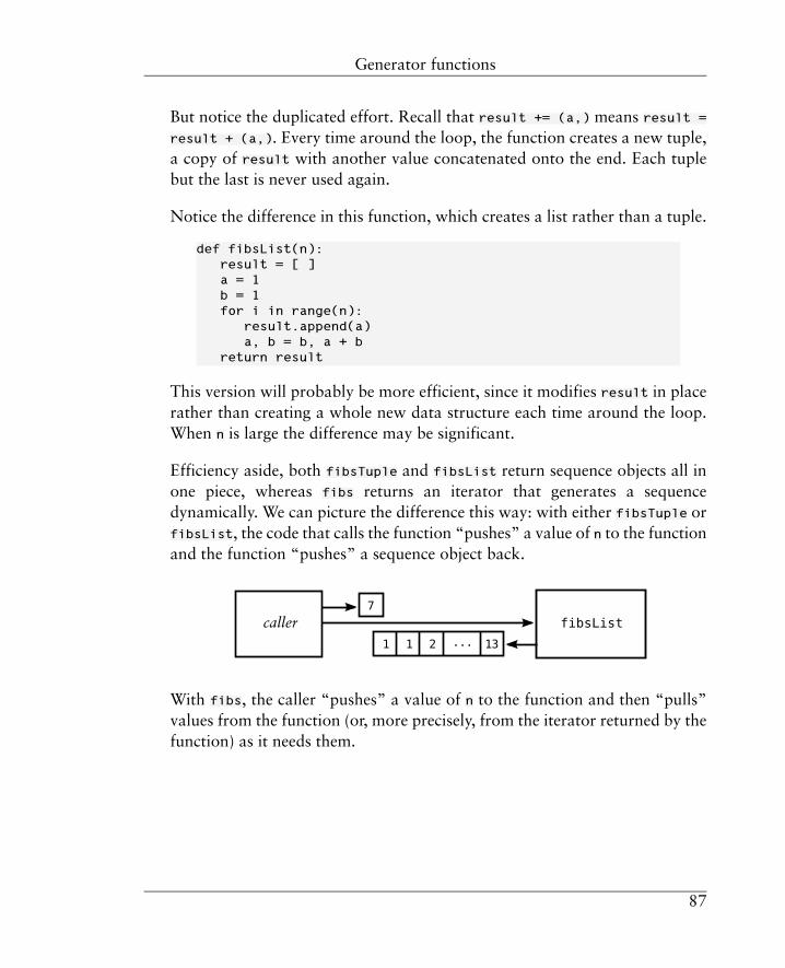
But notice the duplicated effort. Recall that result += (a,) means result =

result + (a,). Every time around the loop, the function creates a new tuple,a copy of result with another value concatenated onto the end. Each tuplebut the last is never used again.

Notice the difference in this function, which creates a list rather than a tuple.

def fibsList(n):result = [ ]a = 1b = 1for i in range(n):

result.append(a)a, b = b, a + b

return result

This version will probably be more efficient, since it modifies result in placerather than creating a whole new data structure each time around the loop.When n is large the difference may be significant.

Efficiency aside, both fibsTuple and fibsList return sequence objects all inone piece, whereas fibs returns an iterator that generates a sequencedynamically. We can picture the difference this way: with either fibsTuple orfibsList, the code that calls the function “pushes” a value of n to the functionand the function “pushes” a sequence object back.

With fibs, the caller “pushes” a value of n to the function and then “pulls”values from the function (or, more precisely, from the iterator returned by thefunction) as it needs them.

87

Generator functions

Recall the map function that we defined in Section 6.4:

def map(f,sequence):result = ( )for a in sequence:

result += ( f(a), )return result

This implementation of map returns a tuple, in much the same way as fibsTupledoes. It computes a correct result, but it has the same efficiency problem thatfibsTuple has. (Did you notice the efficiency problem when we first presentedthis definition of map?)

We mentioned in Section 6.4 that Python has a version of map already definedas a built-in function. That implementation of map is actually a generatorfunction, and it works more like this:

def map(f,sequence):for a in sequence:

yield f(a)

We could include this definition in our own programs in place of the versionthat returns a tuple: not only is it simpler and more straightforward, but it islikely to be more efficient. There is little point, though; we might as well simplyuse the built-in map.

Like map, filter and many other Python built-in and library functions thatoperate on sequences are actually generator functions. They take either staticsequences or streams as arguments and produce streams as results.

88

Generator functions

Just like any other function, a generator function can do more complexcomputations than those in the simple examples that we have seen so far.Furthermore, a generator function can contain yield-statements in more thanone place, to combine the results of more than one computation into a singledynamically-generated sequence. Here is an example.

The generator function combinations, in Example 7.1 below, takes a non-negative integer n and a sequence of different values, and generates all possiblecombinations (as tuples) of elements from the sequence taken n at a time.There are three cases:

• If n = 0, there is only a single result, the empty tuple.

• If n > 0 but the sequence is empty, there are no results. (The Pythonstatement pass is merely a place-holder that does nothing.)

• Otherwise, the function recursively generates combinations of two kinds:the combinations that do not include the first element of the sequence, andthen the combinations that do.

Example 7.1. Combinations using a generator functiondef combinations(n,seq):

if n == 0:yield ()

elif len(seq) == 0:pass

else:first = seq[0]rest = seq[1:]for a in combinations(n, rest):

yield afor a in combinations(n-1, rest):

yield (first,) + a

Take a close look at the code and make sure you see how it works and whyit produces the correct result, especially in the recursive cases. Notice thateach recursive call works its way closer to a basis case, either because the

89

Generator functions

parameter n becomes closer to zero or because the parameter seq becomesshorter.

This computation is a fine example of one that is much easier to do usingrecursion than with iteration. Try to find a solution using only iteration andsee for yourself.

7.3. Endless streamsUsing generator functions it is easy to define streams that never end. Here isa simple example: the function endlessStream takes any value as an argument,and generates an endless stream of repetitions of that value.

def endlessStream(x):while True:

yield x

Here is another example. The function integers generates successive integers,starting from a given initial value.

def integers(n):while True:

yield nn += 1

Again, the stream generated by the function can continue forever, or at leastuntil n becomes too large for Python to store. For all practical purposes, wecan consider the stream endless.

We'll use the word “endless” rather than “infinite” to describe streams thatnever end, to avoid giving the impression that we are somehow computingwith objects of infinite size. Doing that isn't possible in computing as we knowit, of course. An endless stream of the kind that we can generate in a Pythonprogram is simply a sequence that we can take elements from indefinitely,without limit.

It is obvious that endlessStream generates an endless stream. In general,though, it may not be obvious from the definition of a generator functionwhether the stream that it generates is endless or not.

90

Endless streams

Sometimes termination depends on circumstances external to the program.For example, here's a generator function that yields lines from the program'sinput, perhaps coming from a person typing at a keyboard. (The built-infunction input returns the next line from the input, without the terminating“new line” character.) The first empty line terminates the stream generated.

def inputLines():while True:

line = input()if line == "":

return # the stream terminateselse:

yield line

We can't tell by looking at this code whether this generator function will everterminate. It is entirely under the control of the program's user, not theprogram.

Even when termination is entirely under the program's control, it is sometimesdifficult, or even impossible, to tell whether a stream will terminate. Here's asimple example.

Consider the following simple algorithm, which is sometimes called the Collatzalgorithm after the mathematician who proposed it. Start with any positiveinteger n. Then repeatedly do the following:

• If n is even, divide it by 2.

• Otherwise, multiply it by 3 and add 1.

Stop when and if n reaches 1.

Here is Python generator function that implements the Collatz algorithm,generating the stream of values that n takes on for a given starting value.

91

Endless streams

def Collatz(n):yield nwhile n != 1:

if n % 2 == 0:n = n // 2

else:n = 3*n + 1

yield n

For example, with a value of 3 for the argument n, the stream generated is 3,10, 5, 16, 8, 4, 2, 1.

Believe it or not, as this book is being written in 2014 it is still an unsolvedmathematical problem whether the Collatz algorithm terminates for any initialvalue of n. The sequence has terminated for every n ever tried, but nomathematician has been able to prove that it will terminate for any n.

Termination of computations is an important question in computer sciencetheory, as you will see later in your studies if you are a computer sciencestudent. Here, let's just say that it can be difficult or impossible to determinewhether an algorithm will always terminate, given a description of thealgorithm. This is just one of the many reasons that programming can bechallenging.

7.4. Concatenation of streamsAlthough streams are dynamically generated and may be endless, in someways they behave much like any other sequences. Let's look in particular atthe behavior of streams under concatenation.

Let us define the concatenation of two streams X and Y as another stream,generated in the obvious way: by first generating the elements of X and thengenerating the elements of Y.

Here is a Python generator function that directly implements that definition:

92

Concatenation of streams

def concat(X,Y):for a in X:

yield afor b in Y:

yield b

By the way, notice that concat is automatically overloaded for any kind ofsequence that a for-statement can iterate over: strings, tuples, lists, rangeobjects, and iterators. The function can concatenate two streams, or two staticsequences, or one of each. But notice also that each for-loop uses an iteratorto iterate over X or Y, whether or not the object is already an iterator. So concat

is always concatenating two streams in any case. And it always produces astream, not a static sequence.

What does concat(A,B) mean if A generates an endless stream? The result isstill perfectly well-defined; it just never includes any values from B. Thenconcat(A,B) is equal to A; that is, the two expressions generate identicalstreams.

Well, then, is this concatenation operation associative? Certainly it is. It's nothard to see that concat(A,concat(B,C)) = concat(concat(A,B),C) for anystreams A, B and C, endless or not, as follows.

If all of A, B and C generate sequences that end, then the value of the expressionconcat(A,concat(B,C)) is the values generated from A followed by (the valuesgenerated from B followed by the values generated from C). Similarly, the valueof concat(concat(A,B),C) is (the values generated from A followed by thevalues generated from B) followed by the values generated from C. But here"followed by" is ordinary concatenation of finite sequences, which isassociative.

If A generates an endless stream, then concat(A,concat(B,C)) is equal to A

regardless of B and C. But then concat(concat(A,B),C) is equal to concat(A,C)

regardless of B, and so it is equal to A regardless of C; thusconcat(A,concat(B,C)) = concat(concat(A,B),C). And it is easy to checksimilarly that the equality holds in the other cases: when B generates an endlessstream but A does not, and (trivially) when only C generates an endless stream.

93


Another way to see that concat is associative is as follows. Notice that, whenE is a call to a generator function, the for-statement

for e in E:yield e

is just equivalent to the code in the body of the generator function, witharguments to the function substituted into that code appropriately. In effect,the code of the function yields values and the for-statement just passes thosevalues through.

Therefore, the expression concat(A,concat(B,C)) is equivalent to theconcatenation of two code sequences:

for a in A:yield a

for b in B: # all this isyield b # the meaning

for c in C: # ofyield c # concat(B,C)

Similarly, the expression concat(concat(A,B),C)) is equivalent to theconcatenation of two code sequences:

for a in A: # all this isyield a # the meaning

for b in B: # ofyield b # concat(A,B)

for c in C:yield c

But these two segments of code are clearly equivalent. They must produce thesame result, whatever that may be.

So concat is associative. Furthermore, it has an identity: the empty stream.Look at the definition again:

94


def concat(X,Y):for a in X:

yield afor b in Y:

yield b

If X generates the empty stream, the first for-statement terminates immediatelywithout yielding anything and the second for-statement generates whatever Ygenerates, so concat(X,Y) is equivalent to just Y. Similarly, if Y generates theempty stream, concat(X,Y) is equivalent to X.

So the empty stream is an identity for concat. There is only one empty streamvalue, although there are many objects that will generate it: the empty string,the empty tuple, any generator function that terminates without yieldinganything, and so on. The streams generated by all of these are indistinguishablein Python.

The conclusion: streams are a monoid under concat, with the empty streamas identity. By now you should not be surprised at seeing another monoid!

7.5. Programming with streamsLike functional programming, programming with streams gives you a newcollection of techniques for you to add to your repertoire. In this section we'llexplore a few of them.

Whenever you need to do a computation that generates a sequence of valuesso that another computation can iterate over that sequence, think of makingthe first computation generate a stream. Then you can put that computationinto a generator function.

For example, generator functions are handy for generating a sequence of valuesfrom an object, where the object contains the values we want but is structureddifferently. Say that we want to do a computation on every character in a file.As we have seen, a file in Python is a sequence of lines, each of which is asequence of characters. What we want is a different structure: just a sequenceof characters.

95

Programming with streams

Here's a generator function that generates that sequence as a stream. Thefunction takes the name of a file as its argument.

def chars(file):for line in file:

for char in line:yield char

Then we might do the main computation something like this:

f = open(someFileName)for char in chars(f):

main computation using char

Here's a slightly more complicated example. Suppose now that the file is atext file, and suppose that we want to produce a sequence of the words in thefile. This is a structure that is quite different from the structure of the file itself.

We can use the Python method split to separate each line of the file intowords. When split is applied to a string but called with no other argument,it splits the string at “white space”: that is, sequences of space characters and“new line” characters (and other characters that we don't need to consider inthis example, such as tab characters). That's how we would normally dividea line of text into words.

Let's also say that we need to produce the words without any punctuationmarks that might be clinging to the beginning or end of them: commas,quotation marks, and so on. Python has another string method that will dothis. If punctuation is a string containing the punctuation characters that wewant to strip away, the value of word.strip(punctuation) is word with allinstances of those characters stripped from the beginning and end. (By theway, strip treats the characters in punctuation as a set; the description ofstrip in the official Python documentation uses that term.)

Now there's one more complication: if there is white space at the beginningof the line, split will produce an empty string in the sequence of “words”that it produces, and we don't want that effect. The same is true for whitespace at the end of the line, and there will always be at least one “white space”character there, the “new line” character. As it happens, we can use strip to

96


solve this problem too: when called with no arguments other than the string,the method strips “white space” characters.

So here's a generator function that generates a stream of the words in a file.This time we'll put the file-opening operation in the function too, so that thefunction takes a file name as its argument.

def words(fileName):punctuation = ".,:;'" + '"'file = open(fileName)for line in file:

words = line.strip().split()for word in words:

yield word.strip(punctuation)

As in the previous example, we might do the main computation somethinglike this:

for word in words(someFileName):main computation using word

Let's see how the code of this example might look if we wrote it without thegenerator function, and combined everything into one big nested loop:

punctuation = ".,:;'" + '"'f = open(someFileName)for line in file:

words = line.strip().split()for word in words(f):

strippedWord = word.strip(punctuation)main computation using strippedWord

This works just as well, but it doesn't seem as elegant or clear. The maincomputation, which may itself be rather long, is buried in all the clutter offinding words and stripping punctuation. If all that detail is separated out intoa generator function, the part of the program that uses that function canconcentrate on the computation that uses the sequence of words.

By definition, streams are generated dynamically, one element after anotherin time. In fact, the elements of a stream don't necessarily appear at equalintervals in time. Consider the generator function inputLines from Section 7.3,for example. Here it is again:

97


def inputLines():while True:

line = input()if line == "":

return # the stream terminateselse:

yield line

This function generates lines at times that are completely unpredictable, fromthe program's point of view, assuming that the lines come from a humantyping at a keyboard.

Suppose that we want to store input lines typed in that way, but also recordwith each line the time at which it was entered.

We'll need a way of getting the current time from inside a program. The Pythonlibrary has a number of functions for getting and operating on times in differentformats, but we don't need to concern ourselves with the details of thosefunctions here. Let's just assume that we have a function time() that returnsthe current time, in an appropriate format and with sufficient precision forour purposes.

Then here is a function that generates a stream of two-element tuples, eachtuple being the time at which a line was entered and the line itself.

def timedInputLines():for line in inputLines():

t = time()yield (t, line)

This is simple code, but the interesting point about it is the way events unfoldin time. Recall that code that uses timedInputLines will call it to get an iteratorand then "pull" values from that iterator as it needs them. Whenever the codetries to pull a value, timedInputLines can't yield a value until it executes thebody of its for-statement one more time. That causes the for-statement to tryto pull one more value from inputLines. And inputLines can't yield a lineuntil the user has entered one. All this code will sit waiting, if necessary, forthat to happen.

98


As soon as the user has entered a line (assuming that the line is nonempty),inputLines immediately yields it, which causes timedInputLines to executethe body of its for-statement again. Then t gets a time, which is close enough(we hope) to the time at which the user entered the line, and timedInputLines

yields a tuple back to the code that invoked it.

Computations can use more than one stream at a time. Here's an example:Python has a built-in function called zip that takes two static or dynamicsequences X and Y and generates a stream containing elements from X andY paired up, in two-element tuples. For example, the value ofzip((1,2,3),("a","b","c")) is the stream (1,"a"), (2,"b"), (3,"c").

The stream produces by zip terminates when either X or Y terminates. Thismeans that the stream still terminates when either X or Y is endless but theother is not, and this fact leads to some interesting uses for endless streams.For example, we can number the elements in a sequence by zipping them withthe stream produced by the function integers. If y has the value("a","b","c","d"), then the value of zip(integers(1),y) is the stream(1,"a"), (2,"b"), (3,"c"), (4,"d").

Here's an application of that technique. Recall the example in Section 1.2 thatprocessed a file of temperature observations. Suppose we need code that findsall the values in the file observations that exceeded some given value, saythreshold. And suppose we don't want just the values: we want each valuepaired with the position in the file (as a line number) at which it was found.It's not hard to imagine how you would produce this data using ordinarycode, with for-statements and if-statements and so on, but let's do it withstreams in a functional-programming style.

As we have seen, map(int,open("observations")) converts a stream of linesfrom the file to a stream of integer observations . We zip that stream with astream from integers(1), to pair each observation with its position in thefile, and then filter the resulting stream of pairs. Here's all that code as a singleexpression:

filter(lambda a: a[1] > threshold,zip(integers(1),

map(int,open("observations"))))

99


We can picture the various streams in this expression as pipes through whichvalues flow from one function to the next, something like this:

Now let's see how we would write a zip function ourselves if Python didn'talready have one. As it happens, the built-in zip can zip together any numberof sequences, but let's just handle the case of two sequences. So in the definitionof zip(X,Y) we'll want to iterate over X and Y at the same time and generatethe first element of X paired with the first element of Y, then the second elementof X paired with the second element of Y, and so on.

We immediately run into a difficulty: how do we do the iteration in Python?We'd like to say something like "for each x in X and for each y in Y at the sametime", but Python doesn't have a construct for doing such a thing. If X and Y

are static sequences, we can get their corresponding elements by usingsubscripting — say, X[i] and Y[i] for successive values of i — but Pythondoesn't let us do subscripting on streams.

Python does give us a built-in function, called next, that we can call repeatedlyto get successive elements of a sequence. The function is called like this:

next(iterator, endMarker)

Here the argument iterator is an iterator that generates successive elementsof the sequence that we are interested in. As we have seen, a for-statementcreates such an iterator automatically if the sequence object is not already aniterator, but to use next we must create the iterator explicitly. This is doneusing the function iter, which we can use like a type-conversion function,similar to int and tuple and so on. If X is any static sequence or stream object,

100


iter(X) is an iterator for X. It is the same as X if X is already an iterator, so wecan omit using iter if we are sure that this is the case; otherwise we must useiter, even if X is a range object.

The argument endMarker is any distinguished value for next to return to signalthat there are no more elements in the sequence; that is, when iterator

terminates. Of course, endMarker must be different from any value that mightbe in the sequence. Python programmers often use the value None. It's a specialvalue, having a type of its own, that represents "no value"; that is, lack of avalue of any other kind.

So here's the pattern of code that we'll use to iterate over a sequence X usingnext instead of a for-statement: we'll create an iterator using iter(X) and bindit to (say) it, then pull values from that iterator using next(it,None) until weget the value None.

And now let's write a definition for zip(X,Y). We could use next to iterateover both X and Y, but it's a little easier to use a for-statement to iterate overX and work an iteration over Y into that for-statement. Here is one way to doit. Let's assume that we know that None can't be one of the values in Y.

def zip(X,Y):it = iter(Y)for x in X:

y = next(it, None)if y == None:

returnelse:

yield (x,y)

See how zip terminates when X ends (because the for-statement terminates)or when Y ends (because y becomes None and the return statement is executed),whichever comes first. But if both X and Y are endless, so is the result of zippingthem.

Just as we can (in effect) convert a static sequence to a stream by using theiter function, we can convert a stream to a static sequence by using tuple orlist. Either of these type-conversion functions, when applied to a stream,

101


forces the stream to yield all its values at once to be packaged into a staticstructure. Let us call this process materializing the stream.

Why would we ever want to materialize a stream? Perhaps to do someoperation that Python allows on static sequences but not on streams. Onesuch operation is subscripting. Another, if we convert the stream to a list, ismodifying an element in place. We would also probably want to materializea stream if we intend to iterate over its values more than once.

Of course, we must beware of trying to materialize a stream that is endless ormay be endless. For example, if we try to evaluate list(integers(0)), thestream returned by integers(0) will not terminate, and so neither will thecomputation in the list function that tries to materialize the stream. Or, ifwe try to evaluate tuple(inputLines()), the tuple function will not be ableto finish its materializing unless and until the user has typed an empty line.The program will sit and wait until then; it won't be able to process inputlines interactively as the user types them.

If we know, or can compute, how many elements of an endless stream we willneed, we can always materialize just that many elements. For example, if weneed just the first n elements of an endless stream, we can generate a streamof just those elements (see, for example, Exercise 2 at the end if the chapter)and convert the result to a tuple or a list of length n.

In many computations, though, there is no need ever to materialize a streamor a part of it, whether or not the stream is endless. A computation can iterateover the stream directly and control how much of the stream to use, as in ourdefinition of zip.

Thus, in many contexts, endless streams are nothing special. In fact, sometimeswe can get the simplest code by making our generator functions generateendless streams rather than streams that terminate, letting the code that usesthe generator functions determine how much to use.

Here's an example. As we saw earlier in this section, we can number theelements of a sequence by using zip on that sequence and a stream generated

102


by integers. Suppose S is a stream. Then to number its elements starting from0, we could write

zip(integers(0), S)

As we know, integers(0) generates an endless stream of integers startingfrom 0. Now recall that range(n) also generates a sequence of integers startingfrom 0, but only n of them. If we insisted on avoiding endless streams, wecould use range instead of integers, but then we would need to compute thelength of S in advance. And to do that we would need to materialize S first.The resulting code would look something like this:

zip(range(len(tuple(S))), S)

Not only is this code more complicated and probably less efficient, it won'teven work if S can't be materialized.

7.6. Distributed processingAs we saw in Section 6.6, parallel processing is making its way into thecomputer systems that we use every day. But a similar form of processing hasbeen part of our daily lives for years: distributed processing, in whichcomputations on separate computers communicate with each other andcollaborate to produce a larger computation. We use distributed computingevery time we interact with the Internet and the Web, which create a computingenvironment that acts like a single computer with millions of processors.Applications like Web searching and multiplayer games can easily be singlecomputations distributed over computers all around the globe.

Distributed computing is often described as being based on “message-passing”:for example, computer A sends a message to computer B requesting data, andcomputer B sends a message back containing the data. But in fact much of thecommunication in distributed computing is actually based on streams, ratherthan single messages. For example, computer B may be a server that receivesa stream of requests and iterates over that stream, much as in the examplesin this chapter, responding to each request. Or the data returned in responseto a request, unless it is very small, is likely to be broken into a stream of

103

Distributed processing

“packets”, and computer A will iterate over that stream. Some streams of dataare potentially endless, as in audio and video streaming and RSS feeds.

Many computations are distributed simply because data is created or storedin one location but is needed in another. But another reason for distributinga computation is to apply the power of several computers, or even manycomputers, to a single problem.

Should we always distribute computations if we can? Absolutely not; it dependson the computation, and we should avoid using distributed computing forcomputations that are not suited to it. Transferring data from one computerto another over a network is a comparatively slow process, and very slowcompared to the speed of computation on any one computer. So, even if manycomputers are available to help with a computation, it makes no sense totransmit large amounts of data to each computer if each computer will doonly a small amount of computation on that data.

If each remote computer already has its own data, distributed processing maymake more sense. For example, consider a computation on files or web pagesthat are spread throughout a network. Each computer can do its own searchingand aggregating of the data that resides on its own file system, perhaps byusing operations like map and filter and reduce, and then send a relativelysmall quantity of data back to a central computer for aggregating similarlyinto a final result. Or the aggregating can be done in stages, as with thereduction by ⊗ of a0 … a7 that we saw in Section 6.6. Some computers canserve as intermediate aggregators, collecting and aggregating data from severalother computers and sending the results on to another computer to beaggregated further.

Again, a bit of mathematical reasoning can help us design this kind ofdistributed computation for maximum efficiency. For example, if the operationof aggregation is associative, we have more freedom to distribute the operationamong machines and do the operation on parts of the data in parallel. Wehave even more freedom if the operation is commutative; then, for example,an aggregating computer would be able to process results from other computersin whatever order the results may arrive.

104

Distributed processing

Terms introduced in this chapteryield-statementstreammaterializegenerator expressiondistributed processinggenerator function

Exercises1. Experiment with the fib, fibsTuple and fibsList functions of Section 7.2.

Try to find a value of n for which fibsTuple(n) takes noticeably longer torun than fib(n) or vice versa. Repeat with fibsList and fib. If yourcomputer system gives you a way to measure how long a Python programtakes to run, use that; otherwise, just run the Python interpreter interactivelyand observe.

2. Write a generator function prefix(n,stream) that yields the first n elementsof a stream, or the whole stream if its length is less than n. Your functionshould work whether or not the stream is endless, so materializing thestream first is not a solution.

But notice that the stream that prefix returns is not endless in any case,and so it can be materialized if desired.

3. Look again at the integers generator function of Section 7.3. Are we reallyjustified in saying that integers generates an endless stream? Consider youranswers to the first two exercises of Chapter 2.

4. What is the value of each of the following expressions? Be precise in youranswers; distinguish between streams and other kinds of sequences, forexample. Write code that evaluates the expressions to show that youranswers are correct. Assume that map is the built-in function, that doubleis as defined in Section 4.3, and that integers is as defined in Section 7.3.

a. map(double, range(5))

b. map(double, integers(0))

105


c. map(integers, integers(0))

5. In the timedInputLines example of Section 7.5, we assumed that all thecode of the example would sit waiting for the user to enter each input line.What if the input comes faster than the code can consume it? Perhaps theprogram is run in such a way that its input comes from another programrather than from a human at a keyboard, for example. How willtimedInputLines behave?

6. Look again at the averaging-of-temperatures script of Section 1.2. Supposewe have many weather stations at different sites, each taking its owntemperature measurements. Could we distribute the operation of averagingto computers at the weather stations, having those computers send theirresults back to a central computer that would compute one grand average?

106

Exercises

Chapter 8Sets8.1. Mathematical sets

We introduced the concept of a set back in Section 1.3. In this chapter we'lllook at sets in more detail.

Set theory is a central part of advanced mathematics, and set theory can beused to define the foundations of mathematics itself. Set theory, when donewith complete formality, is an abstract and difficult subject. Here we'll describesets much more informally, and concentrate on the concepts of set theory thatare most useful in programming. In the current section we'll briefly andinformally present definitions that we'll need, along with a few interestingand useful facts about sets.

A set is an unordered collection of different things, which we call the membersof the set. The things can be whatever we wish to talk about in a given context,such as numbers or names or people or cities. For example, we can define oneset as all the people in your family, and another set as all the odd numbersless than 100.

In any particular discussion involving sets, we can explicitly define the universeof discourse, meaning all the things, or “elements”, that can be members ofthe sets that we will be talking about; then the set of all these elements is calledthe universal set. Sometimes, though, we let the universe of discourse be definedimplicitly by the things that we happen to talk about, and we don't use theidea of a universal set at all.

In mathematics, the universe of discourse often includes sets themselves, aswell as tuples and other composite mathematical objects. If so, sets can containother sets, as well as tuples and so on.

107

A set is defined by its members. We consider two sets equal if they have exactlythe same members.

We can define a set in several ways. Here are three of the ways:

• By explicitly listing its members. To indicate that a collection is a set, weuse curly braces, so that the set of the numbers 1, 3, and 5 is written

{1, 3, 5}

• By giving a property that the members have. An example is “the set of oddpositive numbers less than 100”. We could express that phrase as

{ n │ 0 < n < 100 and n is odd }

Here the vertical bar “│” is read as “such that”.

The property selects members from some larger “base” set. That set maybe given explicitly as part of the definition:

{ n │ n is an integer and 0 < n < 100 and n is odd }

Or the base set may be left implicit; it may be defined by context, or wemay be meant to assume that it is the universal set.

• By forming the set from other sets using operators, like the union,intersection, and difference operators that we will define below.

There is a set with no members, called the empty set, written ∅ or sometimes{ }.

If an element a is a member of set S, we write a ∈ S. If it is not, we write a ∉ S.For example, 1 ∈ {0, 1, 2} and 1 ∉ {2, 4, 6, 8}.

If every member of a set A is also a member of another set B, we say that Ais a subset of B, written A ⊆ B. For example, {2, 4} ⊆ {1, 2, 3, 4, 5}. But noticethat, by our definition, it is also true that {2, 4} ⊆ {2, 4}; in fact, any set is a

108

Mathematical sets

subset of itself. If we want to say that A ⊆ B but A ≠ B, we say that A is aproper subset of B, written A ⊂ B.

The union of two sets A and B is written A ∪ B, and is another set containingall the elements that are in either A or B or both.

The intersection of two sets A and B is written A ∩ B, and is another setcontaining all the elements (if any) that are in both A and B.

The difference of sets A and B is written A − B, and is another set containingall the elements that are in A but are not in B. (It is also sometimes called the“complement” of B with respect to A, and written A \ B.) For example, {1, 2,3, 4, 5} − {2, 4, 6} is {1, 3, 5}.

Both union and intersection are associative: A ∪ (B ∪ C) = (A ∪ B) ∪ C and A∩ (B ∩ C) = (A ∩ B) ∩ C. Both operators are commutative as well. These factsare not hard to prove; in fact, they follow directly from the fact that we definedunion and intersection using “or” and “and”, and the fact that the latteroperators are associative and commutative in logic.

The empty set is the identity for the union operation; therefore, sets are amonoid under union, with the empty set as identity. If there is a universal set,it is the identity for the intersection operation; then sets are a monoid underintersection, with the universal set as identity. If we have no universal set, setsare still a semigroup under intersection.

In mathematics, sets are often infinite in size; that is, they have infinitely manymembers. For example, mathematicians routinely use the set of all integersand the set of all real numbers. Most of the interesting facts and problems inset theory concern infinite sets.

Furthermore, mathematicians often define sets by giving a property that themembers satisfy, but without showing any way to find those members. Forexample, such a set can be the set of solutions to an equation, like the followingset:

{ x │ x2 - 5x + 6 = 0 }

109

Mathematical sets

Anyone who knows a little algebra knows a method for finding the membersof that set, but the definition of the set doesn't tell you the method. Here'sanother example:

{ (a,b,c,n) │ a and b and c are positive integers, n is an integer greaterthan 2, and an + bn = cn }

It is not obvious how to find members of this set, if there are any. In fact, untilrecently no one knew whether this set was empty, nonempty but finite, orinfinite; but the mathematician Andrew Wiles proved in a 1995 paper thatthe equation has no solutions with the given properties, so we now know thatthe set is empty. (This was the problem of “Fermat's Last Theorem”.)

Compared to mathematicians, we as programmers face obvious limitationson how we can use sets. First, we can't construct infinite sets in our programs.Second, as we noted back in Section 2.3, we must avoid trying to constructsets that are finite but far too large to store in our computers. And, finally, tocreate a set in a program, we must know a method for constructing it. Evenwith these limitations, there are plenty of uses for sets in programming, as wewill see.

8.2. Sets in PythonLike tuples and lists, sets in Python are data structures that can contain otherPython values. The Python term for such a structure is container; Python hasone more kind of container built into the language, the dictionary, which wewill see in Section 9.2.

A Python set, like a static sequence or a stream, is an object that we can iterateover using a for-statement to do something with every member of the set. Anysuch object is called an iterable in Python terminology.

We can construct a set using a set display, which has the same form as a listdisplay except with curly braces instead of square brackets on the outside.The form that explicitly lists the set's members is just like the mathematicalnotation:

110

Sets in Python

{ 1, 3, 5 }

The other kind of set display is a set comprehension, which looks like a listcomprehension except with curly braces instead of square brackets on theoutside. Here's an example, which is one way to construct the set of oddpositive numbers less than 100:

{ n for n in range(100) if n % 2 == 1 }

A set comprehension is the Python way to construct a set by giving a propertythat its members have. In Python we can't just state the property, though; wemust start by building another set or other iterable — range(100) in this case— and then select from it the values with the desired property.

We can also construct a set from a collection of values by using the set typeconversion function, writing set(A) where A is any iterable. (Now that wehave the term “iterable”, we can say that any iterable can also be an argumentto the type-conversion functions tuple and list.) As a special case, the formset() constructs an empty set.

Python has equivalents for all the set operators that we defined in the previoussection. Here is a table of them:

Table 8.1. Set operators

Pythonmath

in∈is a member of

not in∉is not a member of

<=⊆subset

<⊂proper subset

|∪union

&∩intersection

-−difference

Python treats the two-word sequence not in as a single operator. The operators| and & don't look much like the corresponding mathematical operators, but

111

Sets in Python

perhaps you can remember what they mean if you think of them as meaning“or” and “and”; we used those words in our definitions of union andintersection.

Perhaps surprisingly, in Python we can't use {} to denote the empty set. Thisis because {} denotes an empty dictionary. It would probably make more sensefor {} to denote an empty set instead, but Python had dictionaries before ithad sets, so the meaning of {} is historical. To construct an empty set we mustwrite set().

In Python there is no way to construct a universal set of all possible Pythonvalues. Furthermore, in most programming situations, if there is a “universeof discourse” it is either infinite or so large that constructing a universal setfrom its values would be impossible: imagine the set of all Python strings orthe set of all Python integers, for example. But if all the set members in somecontext in your program are values taken from some rather small finite set,you may be able to use that set as a universal set.

Like lists, Python sets are mutable. Like the append method for lists, there isa method add that inserts a value into a set. For example:

setA = { 2,4 }setA.add(3)

After those statements are executed, setA contains the values 2, 3, and 4. If3 had already been in setA, the second statement would have had no effect.

Python has other methods and functions that operate on sets; we'll mentionjust two more here. For a set A and a value x, the statement A.discard(x)

removes x from A; if x is not in A, the statement has no effect. And the functionlen can be applied to sets as well as sequences: len(A) is the number ofelements in A.

As in mathematics, sets in Python are unordered. This means that if you iterateover a set, you will get all the members, but in no particular order. Forexample, if you execute these statements:

112

Sets in Python

cities = { "London", "Paris", "Vienna", "Istanbul" }for place in cities:

print(place)

you might see this:

ParisLondonIstanbulVienna

or you might see the names of the cities in a different order.

Python sets are designed to make testing for membership particularly efficient.This is fortunate, because Python must use membership testing not only todo the in and not in operations, but also to do intersections and unions. Toevaluate A & B, Python does something like this: it tests each member of A tosee whether it is also in B. Similarly, to evaluate A | B, Python does somethinglike this: it starts with the members of A and then tests every member of B,adding the member to the result only if it is not in A.

Python uses a technique called hashing to implement sets. The details ofhashing are beyond the scope of this book, but let's just say that hashinginvolves using the value of an object to compute the object's location in a datastructure. Therefore, to see whether a value is a member of a set, Python simplydoes the hashing computation to see whether there is an object with that valueat the corresponding location. If the set is large, this computation is muchfaster than comparing the given value with each member of the set.

But, once an object is in a set, the object's value can't be allowed to change,since then the value and the object's location in the set wouldn't correspond.Therefore, a Python set can contain only immutable objects. In particular, aset can't contain a list.

Similarly (and unfortunately), a Python set can't contain another Python set.Fortunately, Python has another kind of data structure called a “frozen set”:it behaves like a Python set except that it is immutable. We have seen thattuples behave like lists except that tuples are immutable; the relationshipbetween sets and frozen sets is the same.

113

Sets in Python

To construct a frozen set, we use the type conversion function frozenset; itsargument can be a set, or any other collection of values such as a sequence.To construct an empty frozen set, we write frozenset().

So by converting a set into a frozen set, we get a structure that we can includein another set. For example, in mathematics the combinations of the numbers{0,1,2} taken two at a time is a set of sets:

{{0,1}, {0,2}, {1,2}}

In Python, we can't write it quite that way: the inner sets need to be frozen.We need to write something like this:

{ frozenset(c) for c in ((0,1),(0,2),(1,2)) }

8.3. A case study: finding students for jobsNow let's pause for a short case study, to apply what we have learned so farto a simple data-processing problem.

Suppose that a company is recruiting students at a university to give themjobs after they graduate, and suppose that the company wants to interviewfourth-year students who are either computer science or electrical engineeringstudents and who have a grade average of B or better.

Let's also suppose that the university has data files that will help us find suchstudents. The file cs contains the names of all the computer science students,and the file ee contains the names of all the electrical engineering students.The file year4 contains the names of all the students who are in their fourthyear of study, and the file goodGrades contains the names of all the studentswith a grade average of B or better.

Let's see how we can find the names of all the appropriate students. This is avery easy programming problem, but let's try to find the very best solutionthat we can. We'll start by showing how a beginning programmer mightapproach the problem, and then show how the solution changes as we applyprogressively more of the ideas that we have seen so far in this book.

114

A case study: finding students for jobs

Very early in their programming careers, beginners learn a stereotyped structurefor a program:

1. Read all the inputs.

2. Do the computation.

3. Display the results.

For some programming problems this approach is far too simplistic, but itwill work perfectly well for the current problem.

So let's first consider the task of reading all the inputs. A true beginner mightuse another stereotyped strategy: to read all of a file, read lines one at a timeuntil there aren't any more, using a while-statement with calls to readline

and a test for the empty string, as we saw in an example in Section 3.3.

Insight #1: we don't need to do all that. Reading the file using a for-statementis much easier, as any reader of this book surely knows by now.

So now one way to proceed is to read lines from a file and collect the namesin a data structure. The first structure to come to mind may be a list, especiallyif the programmer is used to programming in a language that isn't quite ashigh-level as Python is. So our strategy might be to start with an empty list,and add each name from the file as we read the lines, like this:

names = [ ]for line in file:

names.append(line.strip())

Insight #2: we don't need to do all that. This kind of computation is exactlywhat a list comprehension is meant for. We can write this instead:

names = [ line.strip() for line in file ]

We can use such a statement to read each of our data files:

year4 = [ line.strip() for line in open("year4") ]cs = [ line.strip() for line in open("cs") ]ee = [ line.strip() for line in open("ee") ]goodGrades = [ line.strip() for line in open("goodGrades") ]

115


Insight #3: there's a lot of common computation here, which we can separateout into a function. Doing this simplifies the code and is generally good practiceanyway. Writing the function is particularly easy in Python, because we canstill use a comprehension and simply let the function return the resulting list.

def listOfNames(filename):return [ line.strip() for line in open(filename) ]

year4 = listOfNames("year4")cs = listOfNames("cs")ee = listOfNames("ee")goodGrades = listOfNames("goodGrades")

Now that we have all the data in data structures in the program, we canproceed with the main computation. The statement of our problem asks usto find “fourth-year students who are either computer science or electricalengineering students and who have a grade average of B or better”. Here isone obvious way to translate that requirement into Python:

candidates = [ ]for student in year4:

if (student in cs or student in ee) \and student in goodGrades:

candidates.append(student)

Insight #4: we can do the same computation more efficiently using sets. Thecomputation does most of its work with the in operator, which Python cando more efficiently on sets than on lists. We'll need to change our code thatreads input so that it creates sets instead of lists, but the changes are obviousand we'll omit them for the moment.

candidates = set()for student in year4:

if (student in cs or student in ee) \and student in goodGrades:

candidates.add(student)

Insight #5: we don't need to do all that. Again, we don't need to initialize adata structure and then add values to it one at a time: we can use acomprehension.

116


candidates = { student for student in year4if (student in cs or student in ee)

and student in goodGrades }

Insight #6: we don't even need to do all that. Now that we have all our namesin sets, why not just use set operations instead?

candidates = year4 & (cs | ee) & goodGrades

Our task is to find “fourth-year students who are either computer science orelectrical engineering students and who have a grade average of B or better”.How could we express the computation any more simply and clearly? Andit's efficient, too.

So, once we put the pieces together and add an obvious for-statement to displaythe results of the computation, here is our program. It's short and simple:

Example 8.1. Finding job candidates using set operationsdef setOfNames(fileName):

return { line.strip()for line in open(fileName) }

year4 = setOfNames("year4")cs = setOfNames("cs")ee = setOfNames("ee")goodGrades = setOfNames("goodGrades")

candidates = year4 & (cs | ee) & goodGrades

for student in candidates:print(student)

For comparison, you might like to write out the program that we would havenow if we had accepted the beginner's solution at each step of the development.

117


8.4. Flat files, sets, and tuplesLet us return to the theme of flat files that we introduced in Section 5.3. Aswe have seen, many flat files represent sets or sequences of values. Often thesevalues are simply numbers or strings, as in the case study of the previoussection or in Example 1.1. In each of those programs, the data files containednames, one name per line, but conceptually each file was a set of names.

More often than not, a program that takes data from such a file will use allthe data in the file. In developing such a program, an obvious first step canbe to write code to get all the data into a data structure in the program. Thefunction setOfNames in the previous section did just that: it took as a parameterthe name of a file, and returned a set of the names in the file. Here is thatfunction with a couple of minor changes.

def setOfValues(fileName):file = open(fileName)return { line.strip() for line in file }

Here the function has a slightly more generic name, to be suitable for usewhen the values in the file are strings of any kind, not necessarily names. (Wemight have been tempted to use just the name “set”, but if we did we wouldn'tbe able to use the built-in set-constructing function with that name.) We putthe call to open in a separate statement, but we could just as well have includedit in the set constructor, as we did in setOfNames. Recall that in this code, asin all examples in this book, we omit the code that would handle situationsin which the file cannot be opened.

The function setOfValues constructs a set from the values in the file, but wecan just as easily construct a list:

def listOfValues(fileName):file = open(fileName)return [ line.strip() for line in file ]

or a stream:

def streamOfValues(fileName):file = open(fileName)return ( line.strip() for line in file )

118

Flat files, sets, and tuples

or a tuple, constructing a stream and then materializing it:

def tupleOfValues(fileName):file = open(fileName)return tuple(( line.strip() for line in file ))

We'll discuss multisets in Section 9.5, and there we'll see what you can do ifyou want to treat the data in a file as a multiset, rather than as a set or asequence.

Now, what if a data file contains lines that are divided into fields? Let'sconsider the common case of CSV files, the “comma-separated values” filesthat we saw in Section 5.3.

As with files of single values, we'll often want to read the whole file and putall of its data into a data structure. For a CSV file, the obvious kind of datastructure is a set, or possibly some kind of sequence, of tuples.

We can split a line into its fields by using the split method:

line.split(",")

So it might appear that we could create the set of tuples that we want usinga comprehension like this:

{ line.strip().split(",") for line in file }

Unfortunately, that solution isn't quite right. It happens that the Python methodsplit produces a list, not a tuple. And we can't construct a set of lists, becauselists are mutable.

The solution is to convert each list that we get from split to a tuple, andconstruct a set from those tuples:

{ tuple(line.strip().split(",")) for line in file }

And here is the obvious function to read a file and give us the set of tuplesthat it represents:

119


def setOfTuples(fileName):file = open(fileName)return { tuple(line.strip().split(","))

for line in file }

Of course, we can just as easily write a function to construct a list, or stream,or tuple of the tuples that we get from the data in the file. We'll assume thatwe have the functions listOfTuples, streamOfTuples, and tupleOfTuples ifwe need them; the definitions are obvious.

Once we have the tuples in any of these data structures, we can iterate overall the tuples using a for-statement. For example, suppose the file directory

is a CSV file in which each line contains a name, a telephone number, and anemail address. We can use code like the following to get each tuple, unpackthe tuple, and then do something with the fields:

directory = setOfTuples("directory")for entry in directory:

(name, phone, email) = entry...

We can also incorporate the unpacking into the for-statement's header. A for-statement binds a name to a value from the stream that it is iterating over,much as an assignment statement binds the name on its left-hand side to avalue. Python lets us bind the elements of a tuple to a comma-separatedsequence of names, in a for-statement header just as in an assignmentstatement:

directory = setOfTuples("directory")for (name, phone, email) in directory:

...

We can also use the for ( ... ) in ... form in a comprehension. Forexample, suppose we have the same file, but we are only interested in thenames and email addresses. Here is one way to construct a set of thecorresponding two-element tuples from the file:

directory = setOfTuples("directory")emailDirectory = { (entry[0], entry[2])

for entry in directory }

120


But the “unpacking” construct lets us give names to the tuple elements, whichmakes the intent of the code clearer:

directory = setOfTuples("directory")emailDirectory = { (name, email)

for (name, phone, email)in directory }

Using a comprehension with filtering (the “for ... in ... if ...” form)we can easily select only certain tuples, or certain fields from certain tuples,as we read the file. For example, consider the example of the previous sectionagain. Suppose that instead of being given the files cs and ee, we are given asingle file students with the names of all students paired with their majorfields of study, something like this:

John Baez,mathJude Collins,CSJoan Denver,CSJoan Denver,EERoberta Dylan,physics...

A student declaring more than one major field of study would have more thanone line in the file, like Joan Denver above. Thus the file represents a relationbut not a mapping, but we don't care about the distinction in this case.

We can construct the sets cs and ee easily as follows:

students = setOfTuples("students")cs = { name for (name,major) in students

if major == "CS" }ee = { name for (name,major) in students

if major == "EE" }

Notice how each comprehension reads easily and has an obvious meaning,but is also concise and easy to write for the amount of work it does.

We can simplify the code a bit by constructing a single set csOrEE containingall the computer science and electrical engineering students, instead of the twosets cs and ee:

121


students = setOfTuples("students")csOrEE = { name for (name,major) in students

if major == "CS" or major == "EE" }

And then we don't need the set-union operation in the main computation. Wecan write this instead:

candidates = year4 & csOrEE & goodGrades

Having made those changes, here's one more easy improvement we can make.Since we aren't going to use the structure students more than once, we don'tneed to materialize it as a set at all: we can leave the collection of tuples as astream, and we can let the comprehension simply iterate over that stream.

With all these changes, our program might appear as shown in Example 8.2.

Example 8.2. Job candidates again, with different input filesdef setOfNames(fileName):

return { line.strip()for line in open(fileName) }

def streamOfTuples(fileName):return ( line.strip().split(","))

for line in open(fileName) )

year4 = setOfNames("year4")csOrEE = { name for (name,major)

in streamOfTuples("students")if major == "CS" or major == "EE" }

goodGrades = setOfNames("goodGrades")

candidates = year4 & csOrEE & goodGrades

for student in candidates:print(student)

You can probably see how to adapt the program to other forms that the inputfiles might have (see Exercise 3, for example).

122


8.5. Other representations of setsEven though Python has sets and a convenient notation for using them builtinto the language, we don't need to use a Python set as the representation forevery collection of data that we view as a set conceptually. We have just seenan example: the names in the file students in the previous section. Conceptuallythose names are a set, because we don't care about their order and we don'texpect duplicates. But their representation in the file is as a static sequence,and as seen by our program they are a stream. Both representations areperfectly appropriate.

Our representation of a set should depend on the operations that we need todo with the set or its elements. A representation as a sequence is perfectlygood if all we need to do is to iterate over all elements of the set, as with thefile students and the files of Examples 1.1 and 1.2. We had no need to convertthe data in those files to Python sets.

Python sets are better representations of conceptual sets if the operations willbe testing values for membership or computing unions and intersections. Notonly does Python have convenient and elegant syntax for these operations,but the operations are implemented quite efficiently by the Python interpreter.

In a programming language without sets and set operations built in,programmers may need to implement those features themselves. Computerscientists have invented a variety of data structures for sets and algorithmsfor set operations. These are beyond the scope of this book, but if you are astudent of computer science you will probably see them later in your studies.Fortunately, many programming languages come with ready-made librariesthat implement sets and set operations. The libraries are not as convenient asthe built-in Python features, but they do the job.

But, in Python or in any other language, it may not be appropriate to use suchheavy-duty machinery just because it is available. Here's another example ofan alternate set representation. Suppose that for some particular purpose ina program we need a set of n different objects or values. The only propertythat they need to have is that they are all different. The only operation on

123

Other representations of sets

them will be to test whether one value is the same as another. We won'tconstruct subsets of them, just use them individually.

It may help us clarify our thinking about the problem to think of the objectsor values as a set while designing the program. But in the implementation, thebest representation of the set members may be simply the integers from 0 ton-1. The set as a whole might be represented as a Python range object, if weneed to iterate over all the members; if not, there may be no need to representthe set explicitly at all. What could be simpler?

Terms introduced in this chapterintersectionmemberdifferenceuniverse of discoursecontaineruniversal setiterableempty setset displaysubsetset comprehensionproper subsethashingunion

Exercises1. Write a Python function that takes as its argument a nonempty set of file

names; the corresponding files contain names of people, as in the examplesof Section 8.2. Your function will return the set of the names that are inall of the files. For example, the files may be a teacher's lists of the studentsin class on different days, and your function will compute the names of thestudents with perfect attendance. Make your code as simple and elegant asyou can.

2. Write a set comprehension that uses an integer value n to produce the setof different factors of n; that is, the set of integers that divide n evenly, notincluding 1 and n itself. Then use this comprehension to define a functionisPrime(n) that returns True if n is prime and False otherwise. An integeris prime if it has no factors.

124


Can you rewrite your isPrime so that it tests only the prime factors of n?It is easy to see that if n has any factors at all it must have prime factors.Also, it is also not hard to see that if n has any factors, at least one mustbe less than or equal to the square root of n; take advantage of that facttoo to cut down the amount of work that your function needs to do.

Which version of isPrime is more efficient? Experiment by timing bothversions.

3. Write a version of the program of Examples 8.1 and 8.2, assuming that theinputs are now these CSV files:

• students, in which each line has three fields: a name, a major field ofstudy, and number of years of study (an integer, 4 for a fourth-yearstudent).

• grades, in which each lines has two fields: a name and a grade average(a number that may contain a decimal point, on a scale of 0.0 to 4.0, sothat 3.0 would represent a B average).

If you find that this exercise is almost too simple to bother with, once youhave seen Examples 8.1 and 8.2, perhaps that's the point of the exercise.

4. For what purposes in a program might you need a set of n objects or valuesthat are all different but need have no other properties, as described at theend of Section 8.5? Try to think of a variety of examples.

125

Exercises

126

Chapter 9Mappings9.1. Mathematical mappings

We introduced the concept of a mapping in Section 1.3. In this chapter we'lllook at mappings in more detail. As we did with sets, we'll describe mappingsvery informally, concentrating on the properties of mappings that will be mostuseful to us as programmers.

A mapping is a set of ordered pairs in which no two ordered pairs have thesame first element. Therefore, a mapping associates a specific second elementwith each value that is the first element of some ordered pair in the set. Inmathematics, “mapping” is a synonym for “function”, and we can use thenotation of functions to define a mapping. For example, to say “f(3) = 7” isto say that the ordered pair (3,7) is in the mapping f.

As with sets, there are a number of ways to define a mapping. One way is tolist the ordered pairs explicitly, like this:

{ (1, 1), (2, 2), (3, 6), (4, 24) }

A common variation on this notation uses the operator ↦ to denote eachordered pair, to emphasize that the first element is mapped to the second:

{ 1 ↦ 1, 2 ↦ 2, 3 ↦ 6, 4 ↦ 24 }

In this notation, each pair a ↦ b is called a maplet.

Mathematicians use a variety of other formal and informal notations to definemappings. For example, here are three ways to define f to be a factorialfunction:

f(n) = n! for all positive integers n

127

f = λn . n! for all positive integers n

f = { n ↦ n! for all positive integers n }

For a given mapping f, its domain, written dom f, is the set of values that arefirst elements of ordered pairs in the mapping. Its range, written ran f, is theset of values that are second elements of ordered pairs in the mapping.1 Noticethat, as in the case of the factorial function, the domain and range of a mappingcan be infinite sets.

Sometimes the domain of a mapping is obvious from context. Sometimes,though, we must specify what the domain is to avoid ambiguity. Take, forexample, the expression “λx . x + 1”. Does it define the successor functionfor non-negative integers, or the function that adds 1 to any real number, orsomething else? Depending on our choice of domain, we get different functions,because the sets of ordered pairs are different.

In mathematics as in programming, a function can take more than oneargument. There are two common ways in mathematics to construct such afunction. The first is to define the function as a mapping from a tuple of valuesto a single value. Consider, for example, a function that maps two numbersto their product:

p(x,y) = xy

Then p could be defined as follows, using the maplet notation:

p = { (x,y) ↦ xy }

With this definition, p(x,y) can be interpreted as shorthand for p((x,y)), sothat, for example, p(2,3) = 6 as one would expect.

1In mathematics there are a variety of terms and definitions for these and related concepts, but theseare the definitions that we will use in this book. Be aware, though, that you might see somewhatdifferent vocabulary in other books.

128

Mathematical mappings

The second way to define a function of more than one argument is as a chainof mappings, each of which maps an argument to a function of the remainingarguments. Here is how p would be defined in this way:

p = { x ↦ { y ↦ xy }}

A function that is defined as a chain of mappings in this way is said to becurried, after the mathematician Haskell Curry.2

With this definition, the value of p(x) is the function of one argument thatmultiplies its argument by x. Then p(x,y) is interpreted as shorthand for(p(x))(y) , so that again p(2,3) = 6 as expected.

But notice that, if p is defined as a curried function, p(x) also has a usefulmeaning by itself: it is like the Python multiplyBy function that we saw inSection 4.3 when we discussed partial application. In general, whenever afunction is defined using currying, partial application of the function to itsarguments (left to right) is defined automatically.

Even though we define a mapping as a set, the usual set operators aren't oftenvery useful. For example, consider f ∪ g where f and g are mappings. Theexpression denotes a set of ordered pairs, but not a mapping except in thespecial case that the domains of f and g don't overlap. The expressions f ∩ gand f − g do denote mappings, but not very useful mappings in most situations.

There are mathematical operators that apply specifically to mappings, andwe'll describe three of them here. One is the domain restriction operator. Fora mapping f and a set A, f│A is f with its domain restricted to A. We candefine it this way:

f│A = { a ↦ b │ a ↦ b ∈ f and a ∈ A }

Another mapping operator is called overriding union or just override. For twomappings f and g, f ⊕ g is f overridden by g; it is a mapping that agrees with

2Yes, feel free to make the obvious puns. Chutney, anyone?

129


g everywhere on the domain of g and agrees with f otherwise.3 We can define⊕ like this:

f ⊕ g = g ∪ (f│dom f - dom g)

Mapping overriding isn't given much attention in mathematics, but it is centralto computation. We can describe a computer's main memory as a mappingfrom locations to values stored at those locations, and any operation thatstores values in one or more memory locations is an overriding of thatmapping. Similarly, elements of a data structure are often accessed by subscriptsor keys. Then the data structure forms a mapping, and any operation thatstores values into the data structure overrides the mapping. We will seeexamples from Python in the next section.

Although the fact may not be obvious at first glance, the override operator isassociative: (f ⊕ g) ⊕ h = f ⊕ (g ⊕ h) for all mappings f, g, and h. And there isan empty mapping, the empty set, and it acts as an identity for ⊕. Therefore(surprise!) mappings are a monoid under ⊕, with the empty mapping as theidentity. But ⊕ is certainly not commutative, because it is asymmetric: mapletsin the second operand take precedence over maplets in the first operand.

We can sometimes use the associative property of overriding to improve theefficiency of updates to large mappings, as found (for example) in databases,or the efficiency of updates to mappings held at remote locations in distributedsystems. A sequence of updates g0, g1, … , gn to a mapping f replaces f by (((f⊕ g0) ⊕ g1) ⊕ … ) ⊕ gn. Especially if all the updates are relatively smallcompared to f, it can sometimes be more efficient to precompute the whole“batch” of updates g0 ⊕ g1 ⊕ … ⊕ gn and then override f with the result. Noticethat the previous expression contains no parentheses; again by associativity,we can group the updates in any way we like, or construct a “big ⊕” operationthat combines them all. Since overriding is not commutative, though, we musttake care to keep the updates in the proper order.

3 The symbol ⊕ is from the Z notation. Z is a mathematical notation, developed at Oxford University,for writing specifications of programs.

130


A third operator on mappings is the composition operator. For two mappingsf and g, their composition is written as g 3 f and is defined as follows:

(g 3 f)(x) = g(f(x)).

In other words:

g 3 f = { (a, c) │ (a, b) ∈ f and (b, c) ∈ g }

One can read g 3 f as “g after f”.

Notice that for a value x to be in the domain of g 3 f, not only must x be indom f, but f(x) must be in dom g.

A mapping f can be composed with itself, which is most useful when ran f ⊆dom f; in fact, we often compose a mapping with itself more than once. Insteadof f 3 f we often write f 2, for f 3 f 3 f we often write f 3, and so on for higher“powers” of f.

9.2. Python dictionariesWe have already seen Python constructs that act like mathematical mappings.Most obviously, a Python function that returns a value is a mapping. But staticsequences — tuples, lists, and even strings — act like mappings too. Recallthat an element of a static sequence S can be accessed by position: S[i] wherei is an integer value in the range 0 to len(S)-1 inclusive. Therefore, we canuse S as a mapping having that range as its domain.

A Python dictionary is another kind of static container that acts like a mapping,but whose domain is not necessarily a range of integers; the first element ofeach ordered pair can be of any of a wide variety of Python types.

To construct a dictionary, we can use a dictionary display that shows theordered pairs explicitly. A dictionary display looks like a set display containingordered pairs, which are written as two values separated by a colon. Here isan example that maps several English names of numbers to their integer values:

numberValue = { "one":1, "two":2, "three":3 }

131

Python dictionaries

In this context the colon acts like the maplet operator ↦ .

The first element of the ordered pair is called a key. To get the value associatedwith a given key in the dictionary, we use an expression of the same form asan expression that selects an element of a sequence by position: the name ofthe dictionary, followed by a key in square brackets. Thus, in the exampleabove, numberValue["two"] would have the value 2.

Dictionary keys can be of almost any Python type; for example, Pythonprogrammers frequently use strings as dictionary keys, as in the exampleabove. But Python uses hashing (Section 8.2) on the key of each ordered pairto store the pair in the dictionary, so a dictionary key, like a set member, mustbe an immutable object. The value associated with the key, on the other hand,can be any Python value.

Python has dictionary comprehensions, which look like set comprehensionsexcept containing ordered pairs using colons. This comprehension, for example,associates each integer from 0 to 49 with its factorial (Section 4.2).

{ n:factorial(n) for n in range(50) }

Python has a number of operations on dictionaries; we'll describe only a fewof them here. For any dictionary d, items(d) is an iterator that yields the key-value pairs in d as two-element tuples, keys(d) is an iterator that yields thekeys of d (that is, the domain of d), and values(d) is an iterator that yieldsthe values associated with the keys of d (its range). To get the number ofordered pairs in d, we write len(d).

The assignment statement d[k] = v associates the value v with the key k in d;it overrides any existing value associated with k if there is one. In mathematicalnotation, it replaces d with d ⊕ { k ↦ v }. If e is another dictionary, d.update(e)overrides d with all the ordered pairs in e; it replaces d with d ⊕ e.

For the programmer's convenience, a few dictionary operations use the keysin a dictionary where one might expect the ordered pairs to be used instead.The Boolean expression k in d tests whether k is a key for some ordered pairin d. As with sets, the in operator uses hashing for efficiency. The expression

132

Python dictionaries

k not in d works similarly. And an operation that iterates over a dictionary,such as a for-statement, creates an iterator over the dictionary's keys ratherthan over its key-value pairs. (As in iterating over a set, the order isunpredictable). In the following example, if codes is a dictionary whose valuesare strings, codesString becomes the concatenation of those strings in someorder.

codesString = ""for k in codes:

codesString += codes[k]

Programmers frequently construct dictionaries from data in flat files, usingcode similar to the code that we presented in Section 8.4 for constructing setsfrom flat files. In fact, we can conveniently use the generator functionstreamOfTuples from Example 8.2 to help in constructing dictionaries fromCSV files. Here is the function again:

def streamOfTuples(fileName):return ( line.strip().split(","))

for line in open(fileName) )

Suppose that addressBook is a CSV file whose lines contains names of peopleand their email addresses. Here is one way to construct a dictionary that mapsnames to email addresses:

address = { name : emailfor (name,email)in streamOfTuples("addressBook") }

And here is one way to construct mappings in both directions, while readingthe file only once for efficiency:

address = {}owner = {}for (name,email) in streamOfTuples("addressBook"):

address[name] = emailowner[email] = name

Now suppose that we want to construct a dictionary in which we use pairsof values to select elements. For example, suppose that populations is a CSVfile in which each line is a triple: the name of a country, the name of a city in

133

Python dictionaries

that country, and the city's population. Sometimes we need both the city nameand the country name to find the correct population figure; for example, Perthin Australia is not the same place as Perth in Scotland. Let's see how toconstruct from the file a dictionary that maps a country and a city to the city'spopulation.

Just as in constructing a mathematical mapping with two arguments, thereare two obvious ways to construct the dictionary that we want. The first wayis to use a 2-tuple of a country and a city as a key. Here's how we might doit:

population = { (country,city) : popfor (country, city, pop)in streamOfTuples("populations") }

Then, for example, we could get the population of Perth in Australia with theexpression population["Australia","Perth"], assuming that the filepopulations contained a line with the corresponding data. Recall that thecomma between the two strings creates a tuple from them; we don't needparentheses.

If you have written programs in other programming languages, you may haveencountered a data structure called a “two-dimensional array”. It may appearthat population is such a structure, accessed by a country in one “dimension”and by a city in the other. But it isn't: it is a “one-dimensional” structureaccessed by a single value, a 2-tuple.

In Python, the more usual way to construct a dictionary accessed by pairs ofvalues is like defining a curried function: by defining a dictionary ofdictionaries. In the current example, we might define a dictionary whose keysare country names, and whose associated values are dictionaries that map citynames to populations. Here is one way to do it. Notice that we must iterateover the tuples twice: the first time: the first for-statement finds the set of thecountries in the data and constructs all the first-level dictionaries.

134

Python dictionaries

population = {}tuples = setOfTuples("populations")for country in { co for (co, city, pop) in tuples }:

population[country] = {}for (country, city, pop) in tuples:

population[country][city] = pop

Then we would get the population of Perth in Australia with the expressionpopulation["Australia"]["Perth"].

You can probably see what you would need to do to construct a dictionaryaccessed by more than two values.

9.3. A case study: finding given words in a file oftext

Let's pause for another case study, to put together a number of the conceptsthat have been presented so far. We'll present a programming problem andthen see how we might choose discrete-mathematical structures for variousparts of the solution.

Suppose we have been given the job of writing the following program:

I need a program that will search an electronic document for a numberof words. For each of those words, the program will display the wordand the line number of every line in the document on which the wordoccurs.

For current purposes, the words will be in a file named “targets”,one word per line, and the document will be in a file named“document”.

Perhaps the person making the request is an author creating an index for abook, or a researcher looking for particular terms in a web page. We'll callthis person “the client”. Let's analyze in discrete-mathematical terms thespecifications that the client gave us.

The words that we will search for are apparently a set.

135

A case study: finding given words in a file of text

The information that the client wants is a mapping from words to collectionsof line numbers. What are the collections? The client says “the line numberof every line in the document on which the word occurs”. If a word occurstwice on a line, the client apparently doesn't want to see the line number twice.So let's make each collection a set so that it won't contain duplicates.

One way to look at the document is as a sequence of lines, each of which isa sequence of words separated by white space. Another way is simply as asequence of words separated by white space, as we did in Section 7.5. But thatisn't enough information in this case, because we'll need to know the numberof the line on which each word occurred. So let's consider a third possibility:we'll treat the document as a sequence of words, each with an associated linenumber; in other words, a sequence of ordered pairs. In fact, we could treatthe document as a set of such pairs — we would get the same result — but,since we anticipate that the document may be very long, we'll plan to treat itas a stream of ordered pairs, generated dynamically as we read the document.

We have already seen how to do some parts of our computation. To constructthe set of “targets”, the words that we are looking for, we can use a simpleset comprehension like one that we used in Section 8.3:

targets = { line.strip() for line in open("targets") }

In Section 7.5 we defined a generator function to generate a stream of wordsfrom a file, removing leading and trailing punctuation from each word:

def words(fileName):punctuation = ".,:;'" + '"'file = open(fileName)for line in file:

words = line.strip().split()for word in words:

yield word.strip(punctuation)

We can easily modify this function so that it counts lines as it reads them, andso that every value that it yields is a two-element tuple of a word and a linenumber:

136


def wordsAndLineNumbers(fileName):punctuation = ".,:;'" + '"'lineno = 0file = open(fileName)for line in file:

lineno += 1words = line.strip().split()for word in words:

yield (word.strip(punctuation), lineno)

A Python dictionary is ideal for representing the mapping that we areconstructing; words in targets will be the keys of that dictionary. We call itlinesFoundOn, and initialize it to map each word in targets to an empty set,using a dictionary comprehension:

linesFoundOn = { t : set() for t in targets }

Then the main computation is very easy using set operations:

for (word,lineno) in wordsAndLineNumbers("document"):if word in targets:

linesFoundOn[word].add(lineno)

Now we display the results. The only hard part is to format each set of linenumbers in an appropriate way. Let's assume that we have a function namedformatted to do that; we'll define formatted later. Using that function, it'seasy to display the results that the client asked for:

for t in targets:print(t + " " + formatted(linesFoundOn[t]))

The only job left is to define formatted, and first we need to decide how wewant to format each set of numbers. The client didn't say anything aboutdisplaying line numbers in any particular order, but we can guess thatascending order might be most convenient for the client. Python has a built-in function named sorted that takes any iterable and returns its values sorted,as a list; we'll use that function. So the definition of formatted will use theexpression sorted(numberSet), where numberSet is the parameter of formatted.

Python also has a built-in function named join that takes any sequence ofstrings and concatenates them into one string, separated by another givenstring. The syntax is separator.join(strings). Let's use a comma followed by

137


a space as a separator. So far we have sorted(numberSet), which is a list ofnumbers; we can convert it to a sequence of strings by writing this:

map(str,sorted(numberSet))

Then we can define formatted like this:

def formatted(numberSet):separator = ", "return separator.join(map(str,sorted(numberSet)))

Putting all the pieces together, we get the program shown as Example 9.1below.

Notice how the program uses examples of all of the following mathematicaland Python constructs:

• streams and generator functions

• 2-tuples

• functional programming with map

• sets and set comprehensions

• mappings, dictionaries, and dictionary comprehensions

See how straightforward and concise each part of the program is as a result.The only slightly messy part is the definition of wordsAndLineNumbers, butthen reading input and taking it apart is often the messiest part of a program.And notice that the whole program is only 19 lines long, not counting blanklines.

Then suppose that the file document contains this brief sample of text:

138


Example 9.1. Finding given words in a documentdef wordsAndLineNumbers(fileName):

punctuation = ".,:;'" + '"'lineno = 0file = open(fileName)for line in file:

lineno += 1words = line.strip().split()for word in words:

yield (word.strip(punctuation), lineno)

def formatted(numberSet):separator = ", "return separator.join(map(str,sorted(numberSet)))

targets = { line.strip() for line in open("targets") }

linesFoundOn = { t : set() for t in targets }

for (word,lineno) in wordsAndLineNumbers("document"):if word in targets:

linesFoundOn[word].add(lineno)

for t in targets:print(t + " " + formatted(linesFoundOn[t]))

Wants pawn term dare worsted ladle gull hoe lift wetter murder innerladle cordage honor itch offer lodge, dock, florist. Disk ladle gullorphan worry putty ladle rat cluck wetter ladle rat hut, an fur diskraisin pimple colder Ladle Rat Rotten Hut.4

And suppose that the file targets contains these lines:

ladlegullhut

4 Howard L. Chace, Anguish Languish, Prentice-Hall, 1956. At the time of writing, available athttp://www.justanyone.com/allanguish.html, which asserts that the copyright of the book has expired.(Try reading the sample text aloud with a bit of a drawl.)

139


http://www.justanyone.com/allanguish.html

Then the output of the program might be as follows.

hut 3gull 1, 2ladle 1, 2, 3

The order of the lines of output is unpredicable; if we want them in alphabeticalorder by word, we could use sorted on the set targets and write this:

for t in sorted(targets):print(t + " " + formatted(linesFoundOn[t]))

9.4. Dictionary or function?As we have seen, we can implement a mapping in a program either as a datastructure (for example, a static sequence or a dictionary in Python) or as acomputation (for example, a Python function). In many respects the two kindsof implementation are equivalent, especially to the program code that usesthe mapping, and in Python the notation for using the mapping is similar inthe two cases. For example, to get the value to which the mapping f maps thevalue a, we write f[a] if f is a sequence or a dictionary and f(a) if f is afunction.

To choose between a data structure and a computation to implement aparticular mapping, a programmer must take into account a number ofconsiderations. Here are some of them:

• Recall that a data structure in a program must be finite in size and alsorelatively small rather than “finite but far too large” (Section 2.3). Acomputation may be the only reasonable choice if the domain of the mappingis very large, such as the set of all Python integers or strings.

• Some mappings in programs must be mutable. This is no problem if themapping is stored as a mutable data structure, such as a list or a dictionary.In most programming languages, program code can't be changed by theprogram itself, or at least not easily. The mapping implemented by acomputation can often be made mutable to some extent, though, if the

140

Dictionary or function?

computation bases its results on data stored in variables or mutable datastructures.

• Once mappings are stored in some data structures such as Pythondictionaries, a program can find the value associated with a value in amapping's domain quite efficiently, often more efficiently than with anotherkind of computation.

• Depending on circumstances, either the implementation as a data structureor the implementation as a computation may be easier to program. Toprogram a mapping as a computation, a programmer must know a methodfor computing the mapping, and preferably a reasonably simple method.Some mappings are so apparently arbitrary that they are most easilyconstructed from explicit data.

But that data must come from somewhere. Small mappings can convenientlybe defined using constructs like Python's dictionary displays, so that thedata is built into the program. More commonly, the data comes from asource external to the program, such as a file or data base. We have seenhow to construct a mapping, as a Python dictionary or sequence, from allthe data in a file. On the other hand, sometimes it can be more efficient toprogram a computation that selectively reads only a small part of a file ordata base to implement a mapping, although we will not present techniquesfor doing so in this book.

Even when there is an obvious computation that defines a mapping, it issometimes useful to precompute the mapping and store the results in a datastructure. Here is an example. Suppose that a Python program has a dictionary-of-dictionaries distance that maps pairs of cities to the distance by road (inkilometers, say) between them. Perhaps distance was constructed from a flatfile, as population was in the second construction in Section 9.2. Then, to getthe distance between two cities, the program would use an expression likedistance[city][otherCity].

Now suppose that the program needs to find a city's nearest neighbor; thatis, for a given city, the other city that is a minimum distance away by road.Here is a function that will do that computation:

141


def nearest(city):# neighborDistance = a dictionary# { each neighbor of city |-> distance to it }neighborDistance = distance[city]

# until we have at least one candidate:nearest = NoneminDistance = float("Infinity")

# for each neighbor of city:for otherCity in neighborDistance:

if neighborDistance[otherCity] < minDistance:nearest = otherCityminDistance = neighborDistance[otherCity]

return nearest

The definition of nearest illustrates several interesting programmingtechniques. First, notice that, since distance is a dictionary of dictionaries (acurried mapping, so to speak), the function can get the mappingneighborDistance by partial application and use it conveniently in thestatements that follow. Second, notice that the function returns the value Nonein the (possibly unlikely) event that distance defines no neighbors for city;it is generally a good idea to program a computation so that it always computesa well-defined value in every situation, however unlikely. Finally, notice howthe Python “infinity” value is used. This is a common use for it: as the startingvalue for a computation that finds a cumulative minimum value.

But notice that nearest does a somewhat time-consuming computation. Thebody of the for-statement is executed once for every neighbor of city. If eachcity has an average of n neighbors, a call to nearest will consume timeapproximately proportional to n on average. If the program needs to callnearest many times, say m times, the total time will be approximatelyproportional to mn, which may be prohibitive if m and n are large.

In some situations it may be a good idea to precompute the values of nearestfor all cities and store the values in a dictionary:

nearestStored = { city : nearest(city)for city in keys(distance) }

142


Then a dictionary access nearestStored[c] will be much faster than a callnearest(c), especially if n is large. It is true that it takes significant time toconstruct nearestStored — approximately proportional to kn if there are kcities — but if m is much larger than k, the overall savings in time will probablybe worthwhile.

It is possible to program a mapping so that it looks up its result in a dictionaryin some cases and uses a computation in other cases. There is an interestingprogramming technique that works this way: it is called memoization. No,that's not a typo! The word is “memo-ization” as in keeping a memo.

The idea of memoization is to store the result of a computation so that, if thesame computation needs to be done again, the stored result can be used instead.In particular, a memoized function, before returning its result, stores the resultin a table using the argument value as a key. If the function is ever called againwith the same argument value, the function returns the stored result from thetable instead of recomputing the result.

As an example, let's consider the function that calculates a Fibonacci number.In Section 7.2 we saw functions that returned sequences of Fibonacci numbers.Now let's consider the function that, given a positive integer n, returns onlythe nth Fibonacci number. As we frequently do in programming, we'll countfrom 0 rather than 1.

Here's a version that calculates the nth Fibonacci number iteratively; that is,by using an iteration. It's a simple adaptation of the function fibs fromSection 7.2. Notice the simultaneous assignment.

def fib(n):a = 1b = 1for i in range(n):

a, b = b, a + breturn a

This function computes a single Fibonacci number reasonably efficiently, butif a program uses it to compute many Fibonacci numbers, the function maywaste a lot of effort. If a program evaluates fib(1000), the body of the for-

143


statement is executed 1000 times. It would be faster to simply use the sum offib(999) and fib(998) if those values happen to be available already.

Let's look at a recursive version of the Fibonacci function. By definition, thefirst two Fibonacci numbers are 1 and 1, and every other Fibonacci numberis the sum of the previous two. Here is a recursive function that is a directtranslation of that definition.

def rfib(n):if n == 0 or n == 1:

return 1else:

return rfib(n-2) + rfib(n-1)

This function works, but it is very inefficient. Notice that the last line of thefunction body computes rfib(n-2) and then rfib(n-1), and the latter recursivecall ends by computing rfib(n-2) again! Similarly, rfib(n-3) is re-evaluatedunnecessarily (more than once, in fact), and so on.

Now here is a memoized version of the recursive function. It saves its resultsin a Python dictionary, which is an ideal kind of container for the purpose.The test in the first line of the function body is very efficient, and if it succeedsthe function simply returns the previously-stored result.

Example 9.2. A memoized function: the nth

Fibonacci numberfibStored = {}

def mfib(n):if n in fibStored:

return fibStored[n]elif n == 0 or n == 1:

return 1else:

result = mfib(n-2) + mfib(n-1)fibStored[n] = resultreturn result

144


All three versions of the function, in the process of computing the nth Fibonaccinumber, compute all smaller Fibonacci numbers. The iterative functioncomputes each only once. Since the memoized function never recomputes aFibonacci number that it has computed before (not counting the trivial 0th

and 1st, which require essentially no computation), it should be approximatelyas efficient as the iterative version in computing a single Fibonacci number.Furthermore, in the process, the memoized function fills in the dictionary withthe results of computing that number and all the smaller Fibonacci numbers.If a program calls the function again with a different n, the required Fibonaccinumber may already be in the dictionary, so that the program gets the numberessentially for free, computationally speaking; and if not, computing thatnumber fills the dictionary with even more results, increasing the chances thatany later call will get its result for free.

9.5. MultisetsWe first saw a multiset in Section 1.3, where we saw that the file of temperatureobservations was a multiset. A multiset (sometimes called a “bag”) hasproperties in common with a set, but it also has properties in common witha mapping, as we will see in this section.

In mathematics there seems to be no commonly accepted notation for multisets,and multisets are often written with the same curly braces that are used towrite sets, so that the multiset that includes 2 twice and 3 once might bewritten { 2, 2, 3 }. In this book we will use different bracketing characters formultisets to distinguish them clearly from sets: we will write the previousmultiset as ⦃ 2, 2, 3 ⦄. This way we can tell unambiguously that (for example){ 2, 3 } is a set but ⦃ 2, 3 ⦄ is a multiset that happens to contain no elementmore than once. (The character ⦃ is the Unicode character called “left whitecurly bracket”, and similarly for the right bracket.)

You may not hear much about multisets in your mathematics classes. In fact,you may hear a lot about sets, but nothing at all about multisets. That'sbecause, to mathematicians, sets are far more important than multisets. Setspervade all of mathematics, from the foundations on up.

145

Multisets

But multisets do have a few important uses in mathematics. For example, theprime factors of a number are a multiset, not a set. Consider the number 360.As you can see by factoring it, 360 is 2 · 2 · 2 · 3 · 3 · 5, so its prime factorsare the multiset ⦃ 2, 2, 2, 3, 3, 5 ⦄.

To take another example, the roots of an algebraic equation can be viewedas a multiset. Recall some simple algebra: the equation x2 - 5x + 6 = 0 can bewritten as (x - 2)(x - 3) = 0, so its roots are 2 and 3. In one way of definingroots, a quadratic equation always has two roots, but they may be the same.For example, the equation x2 - 4x + 4 = 0 can be written as (x - 2)(x - 2) = 0,so its roots are the multiset ⦃ 2, 2 ⦄.

Consider the collection of different items available in a particular shop. Clearly,that's a set. But what about the collection of all the items on the shelves —the inventory? It's a multiset. In taking an inventory, an obvious way toproceed is to take the set of different items and count how many of each itemthere are.

In fact, one way of looking at a multiset is as a mapping from elements to thecount of each. For example, the multiset ⦃ 2, 2, 2, 3, 3, 5 ⦄ can be treated asequivalent to the mapping { 2 ↦ 3, 3 ↦ 2, 5 ↦ 1 }. Then we can get thenumber of occurrences of a value in a multiset, if it occurs there at all, usingfunctional notation; for example, if the previous multiset is m, then the countof 3 in m is m(3) or 2.

Let us define a function count, which gives the number of occurrences of avalue in a multiset, as follows: for a multiset m and a value a, count(m,a) ism(a) if a ∈ dom m and 0 otherwise.5

Using count we can define other operations on multisets. For example, themultiset sum operator, written ⊎, takes two multisets as operands and producesanother in which the counts of elements are the sums of the counts in the twooperands. Multiset union is different: every count is the maximum of thecounts from the operands, rather than the sum. Multiset intersection uses

5In mathematics the term “multiplicity” is often used instead of “count”, but we will use the shorterword.

146

Multisets

minima instead of maxima. In other words, the three operators are definedby these equations: for multisets m and n and element a,

count(m ⊎ n, a) = count(m, a) + count(n, a)

count(m ∪ n, a) = max(count(m, a), count(n, a))

count(m ∩ n, a) = min(count(m, a), count(n, a))

There are two obvious implementations of a multiset in Python: either as asequence of values (a tuple or a list, depending on whether the multiset needsto be mutable), or as a dictionary mapping values to counts. Eitherimplementation has its advantages and disadvantages.

In the implementation as a sequence, the elements have an order but the orderis not important; we use a sequence rather than a set only because a sequencecan contain the same value more than once. The built-in Python method count

is exactly the function count: recall that, if m is a sequence, m.count(a) givesthe number of occurrences of a in m. Python must traverse the whole sequenceto do the counting, though, so the operation can be time-consuming if m islarge. Multiset sum can be simply concatenation. Multiset union andintersection, on the other hand, require more computation: see Exercise 14.

The implementation as a dictionary is probably better if the most commonoperation will be to access counts of elements, as is frequently the case inprograms. Where it is certain that a is in multiset m, the count is simply m[a],which Python can evaluate quite efficiently. In the general case, count mustbe programmed as a function, but the function is simple and again Pythoncan compute it efficiently:

def count(m,a):if a in m:

return m[a]else:

return 0

Multiset sum, union, and intersection require a bit more computation: seeExercise 15.

147

Multisets

It is easy to construct a multiset of the lines of a flat file. For a tupleimplementation, tupleOfValues from Section 8.4 gives us the multiset directly,and similarly for a list implementation. If we want to construct a dictionaryimplementation, we can use streamOfValues from the same section as follows:

def multisetOfValues(fileName):m = {}for a in streamOfValues(fileName):

if a in m:m[a] += 1

else:m[a] = 1

return m

Many other multiset operations that you are likely to need in a Python programwill be simple variations on that code. For example, suppose you want to treatthe lines of a file as integer values, as in the program of Example 1.3. Thefollowing function constructs a multiset of those values:

def multisetOfIntegers(fileName):m = {}for a in streamOfValues(fileName):

n = int(a)if n in m:

m[n] += 1else:

m[n] = 1return m

You can probably see easily how the function would look if you wanted toconstruct a multiset of values from a file transformed in some other way, ora multiset of the values of a particular field in the file lines, and so on.

The if-statement in those functions is a common pattern of code and, packagedas a function on its own, can be useful in many programs:

# tally(m,x):# add 1 to the count of value x in multiset m

def tally(m,x):if x in m:

m[x] += 1else:

m[x] = 1

148

Multisets

In the common situation in which a program uses a multiset as a set ofcounters, the two central operations on the multiset will often be the functionstally and count that we have just defined.

Here's a simple example of a program that uses a multiset as a set of counters.Given the file students that we used in Section 8.4, the program tabulatesand displays the number of students in each major field of study representedin the file. Using the function tally and the function streamOfTuples fromExample 8.2, it's as easy as this:

Example 9.3. Number of students in each major fieldcounts = {}

for (name,major) in streamOfTuples("students"):tally(counts,major) # use major, ignore name

for major in counts:print major + ": " + counts[major}

Terms introduced in this chapterpowers of a mappingmapletdictionary displaydomaindictionary comprehensionrangekeycurried functionmemoizationdomain restrictionmultiset sum, union, intersectionoverriding union, override

composition

Exercises1. Consider the following Python function:

def p(x,y):return x*y

149


Python gives us no way to say that we mean the domain of p to be pairsof integers, or pairs of floating-point numbers, or something else. As itstands, what is the domain of p?

2. Convince yourself, using examples, that the ⊕ operator is associative.Then show why (f ⊕ g) ⊕ h = f ⊕ (g ⊕ h) for any mappings f, g, and h. Usepictures if you like; or, if you can, give a mathematical proof.

3. Consider mappings c and d. Under what conditions on c and d doesc ⊕ d = d ⊕ c?

4. Write a higher-order Python function that returns the composition of twoone-argument functions, as a one-argument function.

5. Write a Python function that returns the composition of two dictionaries,as a dictionary.

6. If f is a function, does the notation f 0 have a sensible meaning? If so,exactly what does f 0 denote?

7. When we defined f 3 as f 3 f 3 f we did not use parentheses in the latterexpression. Was this justified? Is composition of functions associative?Does it have an identity? If so, what is it? Do we have another monoidhere?

8. Which analog of a two-dimensional array — the single dictionary usingordered pairs as keys, or the dictionary of dictionaries — is preferable inPython? Which representation can the Python interpreter operate on moreefficiently? Conduct an experiment: construct two structures, one of eachkind. Then time how long it takes the Python interpreter to access allelements of each structure (to set all the elements to zero, for example).

Discuss what considerations besides speed you might use to decide whichrepresentation to use in a particular program.

9. Look again at the function wordsAndLineNumbers in the program ofSection 9.3. Did it occur to you that this code zips together two sequences

150

Exercises

(Section 7.5)? Rewrite wordsAndLineNumbers using zip. Do you like thisversion of the program better?

10. Modify the program of Section 9.3 so that it finds words in the documentignoring the distinction between upper and lower case letters. For example,with the sample files given, the program would match “hut” in the filetargets not only with “hut” on line 3 of the file document but also with“Hut” on line 4. (Hint: look in the Python documentation for a functionthat will help.)

11. In the nearest function of Section 9.4 we used float("Infinity") as thestarting value in a cumulative-minimum computation. Is it only acoincidence that float("Infinity") is the identity of the monoid of Pythonfloating-point numbers under the minimum-function (Section 6.2)? Whatwould you use as the starting value in a cumulative-maximumcomputation? Can you think of similar computations that you might doin other monoids? How are such computations related to “big” operatorsand to the reduce function of Section 6.4? Can you rewrite nearest usingreduce instead of an iteration?

12. Experiment with versions of the fib function. Is the memoized recursiveversion more efficient than the iterative version? Run each version witha sequence of calls, using a variety of argument values, to give thememoized version a chance to use its stored results.

You should expect that the non-memoized recursive version of the functionwill be much slower than the other two versions for large values of n.Experiment to see how large n needs to be to make the non-memoizedrecursive version impossibly slow.

13. Memoize some other functions and experiment with them to see whetherthe memoized versions are more efficient than the usual versions. Youmight try nearest (Section 9.4), factorial (Section 4.2), or isPrime

(Exercise 2 of Chapter 8). Again, run each version of each function witha sequence of calls using a variety of argument values.

151

Exercises

14. Write Python functions for multiset union and intersection, assuming thatmultisets are implemented as lists.

15. Write Python functions for multiset sum, union, and intersection, assumingthat multisets are implemented as dictionaries. In the dictionaries that thefunctions return, don't include any keys that map to zero.

152

Exercises

Chapter 10Relations10.1. Mathematical terminology and notation

We first saw relations in Section 1.3, where we described relations that aresets of ordered pairs. As we noted in Section 5.3, though, relations inmathematics are more generally sets of n-tuples for any n.

A relation that is a set of ordered pairs is called a binary relation, as we haveseen. There are names for relations that are sets of n-tuples for larger n; forexample, a set of 3-tuples is a ternary relationship and a set of 4-tuples is aquaternary relation. The general term is n-ary relation. As with n-tuples, wecan substitute a specific number for n, so that (for example) a ternary relationis a 3-ary relation. The file populations of Section 9.2 was conceptually a3-ary relation: a set of triples in which each triple contained a city, anothercity, and the distance between them.

If an n-tuple is in a relation, we often interpret that fact as implying that somecorresponding relationship holds among the elements of the n-tuple. Forexample, consider the relation defined by the data in the file emails ofExample 1.2. Call that relation E; then (x, e) ∈ E means that person x hasemail address e.

In mathematics a binary relation is often used as a binary operator: forexample, if (x, e) ∈ E, we can also write x E e. Conversely, a binary operatorthat yields a value of true or false — that is, a Boolean operator — defines abinary relation. For example, the mathematical “=” operator defines a relationthat contains (a, a) for every a in the universe of discourse. (If that universeis infinite, then the relation is an infinite set, which illustrates that relationscan be infinite.) We can even use the operator as the name of the relation, andwrite (a, a) ∈ =.

153

More generally, an n-ary relation defines a predicate, a statement about nthings that is true if the n-tuple of those things is in the relation and falseotherwise. Or, conversely, such a statement defines a relation. The notationof functions is often used for predicates: for example, if P is a 3-ary relationand (a, b, c) ∈ P, then P(a, b, c) has the value true. Similarly, if (a, b, c) ∉ P,then P(a, b, c) has the value false.

Often we use a longer name, rather than a single letter or symbol, for a relationor an operator or a predicate; as we have seen, mathematicians and computerscientists can be rather free in their use of notation. For example, we maywrite “equals” instead of “=”, or “hasEmail” for the relation of Example 1.2.And we often use the notations of relations and operators and predicatesinterchangeably, so that (for example) in each row of the table below all ofthe expressions have the same meaning.

predicateoperatorrelation

E(x, e)x E e(x, e) ∈ E

=(a, b)a = b(a, b) ∈ =

P(a, b, c)(a, b, c) ∈ P

equals(a, b)a equals b(a, b) ∈ equals

hasEmail(x, e)x hasEmail e(x, e) ∈ hasEmail

A 1-ary relation (a set of one-element tuples) is seldom very useful, butpredicates of one argument are common in mathematics. We usually interpretsuch a predicate as a property that a single thing may or may not have, andthen the predicate defines a set rather than a relation: a one-argument predicateP defines the set of all a for which P(a) is true. To take an example fromSection 8.1, suppose that smallOdd(n) represents “0 < n < 100 and n is odd”.Then the predicate smallOdd defines the set of numbers with that property;that is, { n │ smallOdd(n) }.

When a relation R consists of n-tuples whose elements are all members of thesame set A, we say that R is a relation on A. The set is an important propertyof the relation. For example, many binary relations that are important inmathematics and computer science are denoted by binary operators, but if an

154

Mathematical terminology and notation

operator is overloaded we must know the set that the relation is on to knowwhat relation we are talking about. The “<” relation on integers is not thesame as the “<” relation on real numbers, because they are completely differentsets of ordered pairs.

Notice that any relation is always on some set, whether the set is explicitlygiven or not; the smallest set satisfying the definition of “on” is implicitlydefined by the n-tuples in the relation. If the relation is given but the set isnot, and if the relation is finite and reasonably small, we can compute the setfrom the relation.

Mathematicians have identified a number of properties that some binaryrelations have, and we'll mention a few of them here. A binary relation R issymmetric if, whenever a pair (a, b) is in R, then (b, a) is also in R. Forexample, the relation “=” on integers is symmetric, because if a = b, then b =a.

On the other hand, a binary relation R is antisymmetric if, whenever a pair(a, b) is in R, then (b, a) is not in R. For example, the relation “<” on integersis antisymmetric. Notice that from the fact that (b, a) is not in R we can'tconclude that (a, b) is in R; consider the relation “<” and the pair (3, 3), forexample.

A binary relation R is transitive if, whenever (a, b) ∈ R and (b, c) ∈ R, then(a, c) ∈ R. The relations “=” and “<” on integers are both transitive.

If R is a relation on a set A, then we say that R is reflexive if (a, a) ∈ R for alla ∈ A. For example, “=” on integers is reflexive, but “<” is not.

A binary relation that is symmetric, transitive, and reflexive is called anequivalence relation. For example, “=” on integers is an equivalence relation.So is “born in the same year” on pairs of people.

It is not hard to show that an equivalence relation R on a set A defines apartition on A; that is, a set of subsets of A such that every element of A is insome subset and no element is in more than one. The relation R partitions Ainto subsets of elements that R defines as being equivalent to each other.

155

Mathematical terminology and notation

The relation consisting of only (a, a) for all a ∈ A is called the identity relationon A, and is sometimes written IA. Notice that this relation is a mapping; itcan also be called the identity mapping or identity function on A.

Composition of binary relations is defined like composition of mappings(Section 9.1): for two relations R and S,

S 3 R = { (a, c) │ (a, b) ∈ R and (b, c) ∈ S }

Powers of binary relations are also defined as with mappings: for a relationR, we write R2 for R 3 R, we write R3 for R 3 R 3 R, and so on. We define R0

to be the set of all (a, a) and (b, b) for all (a, b) ∈ R; that is, R0 is IA for thesmallest A on which R is defined. We define R1 in the obvious way: it is justR.

10.2. Representations in programsPrograms frequently represent and compute with relations of one kind oranother. In implementing a relation, a programmer faces many of the samechoices as in implementing a mapping or a multiset. Should the representationbe as a data structure, a computation, or some combination of those? If a datastructure, what kind?

In Python, the most obvious representation of a relation is just what thedefinition of “relation” implies: a set of tuples. This representation also hasthe advantage of making some operations particularly convenient, such asiterating through the tuples in the relation or finding whether a given tupleof values is in the relation.

In some situations another representation may be more convenient, though.For example, consider a binary relation containing pairs (a, b). If the mostcommon operation that a program will perform is to find the b valuesassociated with a given a value, it might be convenient to represent the relationas a mapping that maps an a value to a set of b values. On the other hand,this representation makes it rather inconvenient to find the a values associatedwith a given b value, should that operation be necessary too.

156

Representations in programs

Sometimes a computation is a better representation than a data structure fora relation, just as for a mapping and for any of the same reasons (Section 9.4).There are two obvious kinds of implementation as a computation:

• As code that enumerates the tuples in the relation: in Python, a generatorfunction or generator expression, for example. In some situations a streamor other sequence of all the tuples is just what a program needs. Andoccasionally, even if the enumeration would be infinite or very large, aprogram might need only some of the tuples of the relation and could takeonly a prefix of the sequence. Most often, though, the implementation asan enumeration is less useful than the alternative, which is:

• As a predicate; that is, as a function that returns a Boolean value. Such afunction takes n arguments or a tuple of n values and returns True or Falseaccording to whether the corresponding n-tuple is in the relation. Thefunction can do any computation necessary to determine whether it is.

As with a mapping, it can be advantageous to program a predicate partly byaccessing a data structure and partly by a computation. For example, thecomputation can be memoized.

Or we can often make use of special properties of relations, as defined in theprevious section, to infer that some tuples are in a relation even though theyare not stored in the data structure. For example, supppose that a relation r

is symmetric. We can construct a Python set rStored (perhaps from data in afile) that contains pairs (a,b) in one direction, but not the corresponding pairs(b,a) in the other direction. Then we can implement the predicate defining r

by augmenting rStored with program logic as follows:

# predicate r(a,b):# is the pair (a,b) in the symmetric relation r?

def r(a, b):if (a,b) in rStored:

return Trueelif (b,a) in rStored:

return Trueelse:

return False

157


or, more briefly,

# predicate r(a,b):# is the pair (a,b) in the symmetric relation r?

def r(a,b):return (a,b) in rStored or (b,a) in rStored

This technique cuts in half the quantity of stored data we need. Similarly, ifa relation is reflexive, there may be no need to store all the pairs (a,a) for allthe a in the set on which the relation is defined. In situations in which we willonly invoke the predicate for pairs of values that are in that set, we canimplement the predicate like this:

# predicate r(a,b):# is the pair (a,b) in the reflexive relation r?

def r(a,b):return a == b or (a,b) in rStored

We can use similar techniques with relations that are not binary, but that aresymmetric or reflexive in some other sense. For example, consider the examplesin Section 9.4 in which we computed with distances between cities. We cantreat the data in those examples as a 3-ary relation whose triples are two citiesand the distance between them. Since most roads between cities go in bothdirections, the road distance between any two cities is probably the same inboth directions, so the relation is symmetric in that sense. And we can probablytreat the distance from every city to itself as zero, as a kind of reflexiveproperty.

Under those assumptions, we can construct a dictionary-of-dictionariesdistanceStored that contains only distances between different cities in onedirection, and then write a distance function as shown in Example 10.1 below.With this implementation we decrease the amount of data that needs to bestored and possibly the work required to generate the data, at the expense ofincreased computation time and increased complexity of the code. Tradeoffslike this one are common in software design.

158


Example 10.1. Distances using symmetry and reflexivitydef distance(city,otherCity):if city == otherCity:

return 0.0elif city in distanceStored and \

otherCity in distanceStored[city]:return distanceStored[city][otherCity]

elif otherCity in distanceStored and \city in distanceStored[otherCity]:

return distanceStored[otherCity][city]else

return float("Infinity")# no road connection that we have data for

Transitive relations are harder to deal with, and trying to do something similarfor a transitive relation doesn't work. Suppose we want to write a predicater for a transitive relation based on minimal data in a set of pairs rStored. Wewould need to return True for a pair (a,c) if there are pairs (a,b) and (b,c)

in rStored for some b, but how do we find the b? Even worse, we would needto return True for a pair (a,d) if there are pairs (a,b) and (b,c) and (c,d)

in rStored for some b and c, and so on for any longer such chain of valuesthat might exist in rStored. We'll see how to overcome these difficulties inSection 10.4.

10.3. GraphsIn mathematics, a graph is a diagram showing points or other objects andlinks connecting them, or a mathematical object that represents such a diagram.In common English usage we think of a “graph” as a plot of data such as theone in Figure 1.1 (page 15), but in mathematics the term has a specializedmeaning. Here is an example of a graph, shown as a diagram.

159

Graphs

As a mathematical object, a graph is usually defined as an ordered pair (V,E), where V is a set of vertices (the points or objects; the singular is “vertex”)and E is a collection of edges (the links). Starting with this basic definition,there are many variations depending on how V and E are defined. Differentauthors use different definitions and terminology, and different definitionsdefine kinds of graphs with different properties.1 All the definitions that wewill see here use the various structures of discrete mathematics that we havebeen discussing throughout the book, and it is interesting to see how thesestructures can be combined in different ways according to what one wants toexpress in a definition.

In an undirected graph, an edge has no direction and is simply like a lineconnecting two vertices, as in the example above. In a directed graph, eachedge has a direction and is like an arrow from one vertex to another, as in thefollowing example. Edges in a directed graph are sometimes called “directededges” or “arcs”.

1 As always, whatever you're reading, read the definitions carefully!

160

Graphs

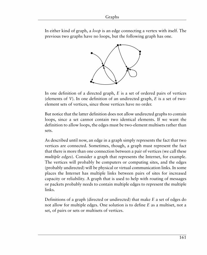
In either kind of graph, a loop is an edge connecting a vertex with itself. Theprevious two graphs have no loops, but the following graph has one.

In one definition of a directed graph, E is a set of ordered pairs of vertices(elements of V). In one definition of an undirected graph, E is a set of two-element sets of vertices, since those vertices have no order.

But notice that the latter definition does not allow undirected graphs to containloops, since a set cannot contain two identical elements. If we want thedefinition to allow loops, the edges must be two-element multisets rather thansets.

As described until now, an edge in a graph simply represents the fact that twovertices are connected. Sometimes, though, a graph must represent the factthat there is more than one connection between a pair of vertices (we call thesemultiple edges). Consider a graph that represents the Internet, for example.The vertices will probably be computers or computing sites, and the edges(probably undirected) will be physical or virtual communication links. In someplaces the Internet has multiple links between pairs of sites for increasedcapacity or reliability. A graph that is used to help with routing of messagesor packets probably needs to contain multiple edges to represent the multiplelinks.

Definitions of a graph (directed or undirected) that make E a set of edges donot allow for multiple edges. One solution is to define E as a multiset, not aset, of pairs or sets or multisets of vertices.

161

Graphs

Some mathematicians take another approach and define a directed graph asa 4-tuple (V, E, head, tail). Here V and E are simply sets of abstract objects,and head and tail are mappings from edges to vertices. An undirected graphhas a single mapping from edges to two-element sets or multisets of vertices.Such definitions allow multiple edges, because any two elements of E aredifferent by definition even though they may have the same ends.

Notice that all of these definitions allow a graph to contain subsets of verticeswith no edges connecting the subsets with each other; there is nothing in anyof the definitions that says otherwise. In fact, there may even be vertices thatare isolated, connected to no other part of the graph.

Unfortunately, the literature of mathematics and computing is not at allconsistent in definitions and terminology regarding graphs. In manymathematics textbooks the term “graph” means an undirected graph withoutloops or multiple edges; where the terms “directed graph” and “undirectedgraph” are used, they often still refer to graphs having no loops or multipleedges. The books may not say so explicitly, but the definitions in the books,like some of the definitions above, imply these facts. In such books, graphsthat may contain loops or multiple edges or both, if they are discussed at all,are given some other name such as “multigraph”.

On the other hand, the term “graph” may be defined so as to allow loops andmultiple edges. If so, the term “simple graph” is often used for a graph withneither.

This confusion of definitions and terminology has sometimes led programmersand computer scientists to make mistakes in their algorithms. For example, a

162

Graphs

programmer may learn a definition of “graph” that is really only appropriatefor simple graphs, and then rely on that definition in constructing a graphalgorithm that should allow for loops or multiple edges but does not. Bewareof such mistakes!

There is an intimate relationship between graphs and binary relations; in fact,we can often view a graph and a binary relation as two different ways ofrepresenting the same information. A directed graph (V, E) defines a binaryrelation on V, sometimes called the adjacency relation of the graph, whichcontains the ordered pair (a,b) if E contains an edge (a,b). Conversely, a binaryrelation defines a directed graph, sometimes called the graph of the relation,that contains an edge (a,b) if the relation contains the ordered pair (a,b). Anundirected graph defines a symmetric relation, and vice versa, similarly. Butnotice that none of these relations can represent any multiple edges that maybe present in the corresponding graph.

In a program, the edge set of a directed graph without multiple edges can berepresented in any of the ways that a binary relation can, as described in theprevious section, and the same design considerations apply. If the graphcontains multiple edges, similar representations are possible where a multisetof ordered pairs replaces the binary relation. If the graph is undirected, therepresentation can be like that of a symmetric directed graph, with a directededge in each direction for each edge in the undirected graph. Otherrepresentations are sometimes useful to facilitate particular computations ongraphs, such as the computations that we will consider in Section 10.4, andwe will see a quite different representation in Section 11.6.

Graphs can be augmented to contain additional information. For example, alabeled graph is a graph in which the vertices or edges or both have identifyinglabels, such as names or numbers. For example, in a graph representing a roadmap, the vertices might be labeled with names of cities and the edges mightbe labeled with names of roads.

In a directed graph with labeled edges, an edge can be defined as a triple oftwo vertices and a label. If every edge has a different label, the problem ofmultiple edges largely goes away: the collection E of edges can again be defined

163

Graphs

as a set, and multiple edges between two vertices are distinct members of theset, distinguished by their labels. Similar comments apply to undirected graphswith labeled edges. In a graph with labeled vertices in which every vertex labelis different, the label of each vertex can sometimes be a convenientrepresentation of the vertex in a program.

A weighted graph is a graph in which each edge is associated with a number,called its “weight”. The meaning of the weight depends on what the graphrepresents. For example, in a weighted graph in which the vertices representcities, the weight of an edge may represent the length of a road between twocities, as in the examples of Section 9.4, or the time needed to travel betweentwo cities by train or air. The dictionary-of-dictionaries in Example 10.1 showsone way to define a weighted graph and represent it in a program: essentially,using a mapping from edges to weights. In that example the edges are pairsof vertices; apparently there are no multiple edges. If that is the case, anotherrepresentation of the graph could be as a set of triples, each triple being twovertices and a weight. But in the presence of multiple edges this representationwould not work, because usually there is no reason to believe that all theweights are different.

A graph can be both labeled and weighted. Graphs that are labeled or weightedor both are common in computational problems.

10.4. Paths and transitive closureIn computing, one of the most common operations on graphs (directed orundirected) is to find paths from one vertex to another. A path in a graph canbe defined as a sequence of vertices such that there is an edge in the graphfrom each vertex to the next, and a path between two vertices a and b can bedefined as a path beginning at a and ending at b. Alternatively, a path can bedefined as the sequence of edges, and this is the definition that we will usuallyuse. We will also say that there is a path of length zero, the empty sequenceof edges, from every vertex to itself. Not all mathematicians would allowempty paths, but if we allow empty sequences it makes sense to allow emptypaths, and the generalization can be useful for avoiding special cases incomputer algorithms.

164

Paths and transitive closure

Many programs need to compute answers to questions such as these:

• For a given graph and vertices a and b in it, is there a path from a to b?

• If so, what is the length of the shortest path, meaning the path with thefewest edges?

• Or, if the graph is weighted, what is the length of the minimum-weightpath, meaning the path with the smallest sum of weights?

• Does the graph contain a cycle, meaning a nonempty path from a vertex toitself? Does the graph contain a cycle that includes some given vertex?

• If the graph is labeled, what is a path (if any) that answers each of the abovequestions, as a sequence of labels?

• Is the graph connected: is there a path from each vertex to every othervertex?

Some obvious examples of programs that do computations like these are thepopular programs that give driving directions for the fastest route betweentwo cities, and programs that route messages or packets from one site toanother in the Internet.

We can gain insight into the questions above by considering the adjacencyrelation of a graph instead of the graph itself, and by considering the transitiveclosure of that relation. The transitive closure of a relation R is defined as thesmallest relation containing R which is transitive; that is, the relation we getby adding to R all the ordered pairs implied by the transitive property and noothers. The transitive closure of R is often denoted as R+.

One way to find the transitive closure of a relation R is to build it up iteratively.We start with R. Then we find R2: for every pair (a, b) in R, we find everypair (b, c), and the set of pairs (a, c) is R2. We add that set to our result; wenow have R ∪ R2. Now we find R3 by composing R and R2 similarly, and addR3 to our result. We continue in this way; then finally we get R+, which is R∪ R2 ∪ R3 ∪ …

165


If R is a finite relation (that is, a finite set of pairs), we do not need to computean infinite union to find R+: eventually no new pairs will be added to theresult, and we can stop. The set of all a and b such that (a, b) ∈ R is a finiteset, and there are only finitely many possible pairs of members of that set.Therefore, we will eventually reach a k such that every pair in Rk+1 is alreadyin R ∪ R2 ∪ R3 ∪ … ∪ Rk. We can terminate the iterative building of R+ whenthis is the case. Thus the method described above is a sketch of an algorithmfor computing R+, guaranteed to terminate if R is finite. We will call it theObvious Algorithm for transitive closure.

Now notice that if R is the adjacency relation of G, pairs in R2 are end pointsof paths of length 2 in G, pairs in R3 are end points of paths of length 3 in G,and so on. Then R+ is the set of pairs of vertices (a, b) such that there is a pathof any nonzero length from a to b in G.

So if G is finite, we can compute R+, and it contains the information we needto answer many of the questions about paths that we listed above. Manyvariations on the Obvious Algorithm are possible depending on the questionwe want to answer. For example, if we are only interested in paths startingat a given vertex a, we don't need to compute the whole relation R+; we canstart with only the relation { (a, b) │ (a, b) ∈ R for some b } and repeatedlycompose that relation with R as in the Obvious Algorithm. For questionsinvolving labels or weights, we can modify the Obvious Algorithm to keeptrack of the labels and weights associated with each path we find.

The Obvious Algorithm is not the most efficient algorithm for computing atransitive closure in all situations or for all kinds of relations or graphs, andit is not really practical at all for large relations or graphs. Computer scientistshave studied transitive closures and paths in graphs extensively, and there isa substantial literature describing improved algorithms, as well as datastructures that make the computations easier. All of these results are beyondthe scope of this book, but if you are a computer science student you willprobably see some of them later in your studies. And if you ever need to writea serious program involving transitive closures or paths in graphs, especiallyif the amount of data is large, you should probably investigate the literaturebefore getting too far into designing the program.

166


Other closures are possible besides the transitive closure. For example, thesymmetric closure of a relation R is formed by adding to R the pair (b, a) forevery (a, b) ∈ R. The reflexive closure of a relation R is formed by adding toR the pairs (a, a) and (b, b) for every (a, b) ∈ R.

The reflexive transitive closure of a relation R is the reflexive closure of R+;it is often denoted as R*. Then R* = R0 ∪ R1 ∪ R2 ∪ R3 ∪ … . If R is theadjacency relation of a graph G, there is a pair (a, b) in R* whenever there isa path, empty or not, from a to b in G.

Transitive closures and reflexive transitive closures have many uses inmathematics and computer science besides finding paths in graphs but, again,those uses are outside the scope of this book. The main purpose of the currentsection is to introduce you to concepts so that you will start thinking alongthe right lines whenever you see a programming problem that can be solvedby finding closures or paths in graphs.

By the way, the superscript “+” and “*” are common idioms in computerscience and mathematics, and are used to mean “one or more times” and“zero or more times”, respectively, in all kinds of contexts. A computer sciencestudent soon learns that a superscript “*” is not necessarily an instruction tolook for a footnote at the bottom of the page!

10.5. Relational database operationsNow that we have looked at relations in a bit more detail, let us return to thetopic of relational databases.

As we mentioned in Section 5.3, a relation in a relational database is verymuch like a mathematical relation, being a set of “tuples”. However, in arelational database tuple, the elements are identified by name rather than byposition.

In the terminology of relational databases, one property of a relation is theset of attributes of its tuples. Each attribute has a name, and a tuple is a setof named attribute values.

167

Relational database operations

We can describe a database relation in terms of a mathematical relation plussome additional information about attribute names. Let us represent a databaserelation with n attributes as a triple (R, A, col), where R is an n-arymathematical relation, A is a set of n attribute names, and col (for “column”)is a mapping from attribute names to positions, which are integers in the range0 to n-1. For a particular database relation, say X, we can call the componentsof the representation RX, AX, and colX.

In the representation, some order is chosen for the attributes, and the tuplesin R all have their attribute values in that order. Then R is like a table, withtuples corresponding to rows and attributes corresponding to columns. Theorder of the attributes defines the mapping col.

In a small and simple relational database, relations could be implementedmuch as the above description would suggest. For example, the R of a relationcould be represented in a program as a set of tuples, and in a file system as aflat file. However, the implementation of a real, production-quality relationaldatabase system is usually much more complicated, with additional datastructures and algorithms to make access and operations more efficient. Allthis complexity is, once again, beyond the scope of the current book. Herewe'll just use our representation (R, A, col) to talk abstractly about databaserelations and operations on them, and to help us picture what is going on.

Relational database operations are designed to allow users, often managersand information technology staff in organizations, to combine and extractinformation contained in relations in a database. We'll describe a few of themost important relational database operations informally here.

Relation union, intersection, and difference are defined much like thecorresponding operations on sets of tuples. These operations on two relationsX and Y make sense only if the relations have the same attributes; that is, wemust have AX = AY.

Let us picture Y′ as the relation we would get by reordering the “columns”of Y, if necessary, so that the attributes are in the same order as in X. ThusAY′ = AX, colY′ = colX, and RY′ is RY with the values in each tuple reorderedto agree with colX.

168


Then the union of relations X and Y is another relation Z, defined as follows:RZ = RX ∪ RY′, AZ = AX, and colZ = colX. The intersection and difference of Xand Y are defined similarly.

In implementing these operations, we could just as well choose to reorder thefirst relation rather than the second. But the implementations would be simplerif no reordering of either relation would ever be necessary. To ensure that thisis the case, we could define a standard ordering of attributes for all relationsin the database: alphabetical by attribute name, for example.

A very common database operation is selection: to select from a relation alltuples that meet some criterion. This operation is very much like the filter

function that we first saw in Section 6.4, and like filtering using “if” in Pythoncomprehensions. In mathematical notation a selection is written as σP(X),where X is a relation and P is a predicate or Boolean-valued expression (hereσ is a lower-case Greek sigma). The result is a new relation. For example,consider this relation from Section 5.3:

If this relation is X, and if P is “project = ‘Alpha’”, then σP(X) is

Often a database manipulation needs only some of the “columns” of a relation.A projection of a relation is a new relation containing a subset of the attributesof the original relation. In mathematical notation, a projection is written asπS(X), where X is a relation and S is a set of names of attributes to be included

169


in the result (here π is a lower-case Greek pi). For example, if X is as aboveand S is { “name”, “lab” }, then πS(X) is

There are a number of operators for combining information from more thanone relation. The most important of these is the natural join. If Y and Z arerelations, their natural join, written Y 9 Z, is created from pairs of tuples inY and Z that agree in values of the attributes that the two relations have incommon. The resulting relation contains tuples whose attributes are the unionof the attributes of the pairs of tuples from Y and Z. For example, let X be asabove and let W be this relation:

Then X 9 W is

170


By the way, the operator 9 is sometimes called the “bowtie operator”.

Using natural join and projection it is possible to perform an operation thatis much like a mathematical composition of relations. For example, considerthe two-attribute database relations πS(X) and W above: they are much likemathematical binary relations. Combining them with a natural join, we obtain

Then we perform a projection to remove the common attribute, and we obtain

This result is the relational database equivalent of W 3 πS(X).

Terms introduced in this chapterloopn-ary relationmultiple edgespredicateadjacency relationrelation on a set

171


graph of a relationsymmetric relationlabeled graphantisymmetric relationweighted graphtransitive relationpathreflexive relationtransitive closureequivalence relationsymmetric closurepartitionreflexive closureidentity relationreflexive transitive closureidentity mapping/functionattributerelation compositionrelational union, intersection,power of a relation

differencegraphselectionvertexprojectionedgenatural joindirected graph

undirected graph

Exercises1. Obviously IA is reflexive for any set A. Is it transitive? Is it an equivalence

relation?

2. In Section 10.3 we gave a very informal definition of the “graph of arelation”, but in that definition we described only the set of edges of thegraph. What is the set of vertices? Is there more than one possible choice?

3. Write a Python function that returns the transitive closure of a relation,where the relation and the result are Python sets of two-element tuples.

4. If G is a finite graph and R is its adjacency relation, and if you computeR+ using the Obvious Algorithm, what is k, the number of powers of Rthat the algorithm will compute before terminating? Can you find anapproximate value, an upper bound, or even an exact value? Express youranswer in terms of paths in G. This k will usually be much less than thenumber implied by the argument that there are only finitely many pairsthat R+ can contain.

172

Exercises

5. In a given directed graph, if the vertex at the end of one path is the sameas the vertex at the beginning of another path, the two paths can beconcatenated to form another path in the graph. Is the set of all paths in agiven directed graph a monoid under concatenation?

6. What is σP(X) expressed as a triple? In other words, what are its R, A andcol? Assume that you can use P as a predicate, writing expressions like“P(x)”.

Repeat for πS(X) and X 9 Y. These are a bit harder, at least if you do thementirely in mathematical notation.

7. What are some properties of the natural join operation? Is 9 associative?Is it commutative? Does it have an identity? Do we have another monoidhere?

173

Exercises

174

Chapter 11Objects11.1. Objects in programs

We have used the term “object” in previous chapters, but we have not yetdefined exactly what we mean by “object”. The term has a specific, commonly-understood meaning in programming, although details of definitions andterminology vary from one writer to another and from one programminglanguage to another. Here we will present informal definitions and terminologythat are typical in the programming-language world, and that (in particular)agree with Python's treatment of objects.

An object is a piece of data that typically has a number of attributes, identifiedby name, much like fields in a tuple in a database relation (Section 10.5). Forexample, an object representing a person might have attributes “name”,“address”, and “department”. Objects in a program often represents thingsin the real world, and then an object's attributes are properties of the thing.

Thus a programming-language object is another kind of container for data,but one in which the elements of data are identified by name rather than bya position or a key. Often an object is mutable: values of its data attributescan be changed. For example, a program may allow the address attribute ofa person object to be changed. The collection of the values of all the dataattributes of an object at any time is called the state of the object. To say thatan object is mutable, then, is to say that its state can change.

Other attributes of an object, besides the attributes that store data, areoperations that can be performed on the object. These operations are calledmethods. A method of an object, like a data attribute of an object, “belongsto” the object. Methods of different objects, as well as data attributes ofdifferent objects, may have the same name but may mean different things andmay be implemented differently. These facts are central to object-orientedprogramming, which we will describe in a bit more detail in Section 11.4.

175

In most programming languages an object is of a particular type or belongsto a class of similar objects. Object-oriented programming languages provideways for programmers to define their own classes of objects. The type or classof an object determines what attributes (both data attributes and methods)the object has.

We can view an object as a mapping from attribute names to values, much asa relational-database tuple is a mapping from field names to values (recallSection 5.3). But, turning things around, we can view an attribute of a classas a mapping from objects of that class to values. For example, the attribute“name” might map a “person” object to a string, the name of that person.So, if our program needs a mapping from “person” objects to names, we haveseen two options so far (Section 9.4): we could define a function that takes a“person” object as a parameter and returns a name; or we could build a datastructure (such as Python dictionary) that takes a “person” object as a keyand produces a name. Now we have a third option: to store the name as anattribute of the “person” object.

An object is more than a collection of attributes, though. In a typicalprogramming language, an object has an identity that belongs to that objectalone. The identity of an object never changes, even if the object is mutable;on the other hand, two objects may be of the same type or class and have allthe same attributes and state but be distinguishable by their identities. (Oftena programming language interpreter or compiler will use an object's locationin memory as the identity of the object.)

In Python (and in many other programming languages), the syntax for accessingan attribute of an object is of the form object . attribute. For example, if bossis a “person” object, boss.name would be the “name” attribute of that object.

In the case of a method, object.method is a function. In Python, the syntaxfor calling a method is object.method(arguments). When Python executes thecall, the object is treated as one argument to the function (we will see howthis works in Section 11.2). We say that we apply the method to the object,passing the values in the parentheses as additional arguments.

176

Objects in programs

Typically, a method uses or operates on data attributes of the object; forexample, the call boss.changeAddress(addr) might set the address attributeof boss to addr, and the call boss.addressLabel() might return a stringcontaining values of data attributes of boss formatted in a way appropriatefor printing as an address label. Notice that in the latter case the method callpasses no additional arguments, which is not too unusual.

11.2. Defining classesOne key characteristic of object-oriented programming languages is that thelanguages allow programmers to define their own classes of objects. We willshow how this is done in Python.

A class definition is a compound statement, whose header looks like this:

class classname :

The body of the class definition contains function definitions, which definemethods, and possibly other statements.

A class definition, when executed, implicitly defines a function for creatingobjects of the class; these objects are called instances of the class. The functionis called the constructor for the class, and has the same name as the name ofthe class.1

Different instances of a class have different identities. The binary operator iscompares the identity of two objects; an expression of the form a is b has thevalue True if a and b are the same object and False otherwise. The operatoris not has the opposite meaning.

A class definition may contain a definition of a method with the special name“_ _init_ _”. The _ _init_ _ method is used to initialize newly-created objects.When a constructor is called, it first creates an object and then calls the

1This description is a slight simplification of what really happens in Python, but it will be good enoughfor our purposes.

177

Defining classes

_ _init_ _ method if the class has one. Programmers find this feature of Pythonso useful that most programmer-defined classes have _ _init_ _ methods.

The constructor passes the newly-created object to the _ _init_ _ method asan argument. If the constructor is called with arguments, it passes thosearguments to _ _init_ _ as additional arguments.

Here's a simple example of a class definition:

class Person:

def _ _init_ _(self, name, dept, address):self.name = nameself.department = deptself.address = address

This code defines a class whose constructor is called with three arguments: aname, an address, and a department (possibly all strings). The constructorcalls the _ _init_ _ method with four arguments: the newly-created objectfollowed by the three arguments passed to the constructor. In this _ _init_ _method, the object is called self. The word self is not a keyword and hasno predefined meaning in Python, but it is a common programming conventionamong Python programmers to use the name in this way. (By the way, anothercommon convention is to capitalize the names of programmer-defined classes.)

This _ _init_ _ method sets the values of data attributes of the new Person

object from the arguments passed to the constructor; this is a common thingfor _ _init_ _ methods to do.

In this example two of the data attributes have names that are the same asnames of parameters to _ _init_ _. The two uses of “address” (for example)refer to different things; there is no ambiguity because of the way that Pythoninterprets names. A class defines its own name space, which is a mapping fromnames to things bound to those names.2 The name space of a class containsthe names of data attributes and methods of the class and anything else createdwithin the body of the class definition. A function definition creates anothername space, which contains the function's parameters and any names of

2 Python uses its own dictionaries to construct the mappings for its name spaces.

178

Defining classes

variables and other things created within the function body. These name spacesare distinct from the “global” name space, which contains the names of things,such as variables and functions, that are defined outside class definitions andfunction definitions.

In the statement self.address = address (for example), the “.” operatorfinds the class of self, which is Person, and looks for “address” in the namespace of that class. Since “address” on the right-hand side of the assignmentstatement occurs without the “.” operator, it is not a reference to an attributeof a class, so Python looks for it in the name space of _ _init_ _. The twooccurrences of “address” refer to completely different things, as if theprogrammer had used two different names.

Now suppose we create a Person object, perhaps like this:

boss = Person("Malone", "IT", "127 Spring")

The constructor is called, _ _init_ _ is called, and then (for example) the valueof boss.name would be "Malone".

To define an ordinary method of a class, we write another function definitionwithin the body of the class definition, like this:

class Person:

def _ _init_ _(self, name, dept, address):self.name = nameself.department = deptself.address = address

def addressLabel(self):return self.name + "\n" \

+ self.department + " Department\n" \+ self.address

To use the addressLabel method, we would apply it to a Person object, perhapslike this:

toTheBoss = boss.addressLabel()

179

Defining classes

Then the object boss is bound to the parameter self in addressLabel; in thisexample there are no additional arguments. As in _ _init_ _, it is conventionalbut not required to use “self” as the name of the first parameter to ordinarymethods of a class.

The same program might contain a definition of another class, say Building,that has a different collection of attributes; for example, a Building mighthave a name and an address but not a department. And Building might havemethods that Person does not have, and vice versa. Also, Building might havean addressLabel method, but its definition might be different from that ofthe addressLabel method of the Person class. There would be no ambiguity,because each class has its own name space.

11.3. Inheritance and the hierarchy of classesA key feature of object-oriented programming languages is inheritance, whichallows a programmer to create a new class based on an existing class. Typically,the new class is the old class with features added. Again, we will use Pythonto illustrate the concept.

Suppose that we want to define a class called Customer. A Customer object islike a Person object, but it has an additional attribute: the company that thecustomer represents.

We could define another class using a definition much like the definition ofthe Person class, but in which the _ _init_ _ method takes an additionalargument and creates another attribute of the newly-created object, perhapslike this:

class Customer:

def _ _init_ _(self, name, company, dept, addr):self.name = nameself.company = companyself.department = deptself.address = address

But using inheritance we can reuse the definition of Person in the definitionof Customer, by referring to Person in the header of the new class definition:

180

Inheritance and the hierarchy of classes

class Customer(Person):

Then we say that the class Customer inherits from the class Person. We saythat Customer is a subclass of the Person class, and that Person is the superclassof the Customer class.

In the _ _init_ _ method of the class Customer, we call the _ _init_ _ methodof class Person to do whatever initialization needs to be done for any Person

object, and then we do any initialization that is specific to Customer objects.To get the _ _init_ _ method of the Person class rather than the _ _init_ _

method currently being defined, we apply _ _init_ _ to the name of the class,passing the newly-created object and any other arguments that the _ _init_ _method of that class expects.3 This is how the code might look:

class Customer(Person):

def _ _init_ _(self, name, company, dept, addr):Person._ _init_ _(self, name, dept, addr)self.company = company

Then a Customer object has a company data attribute, and also all the attributesof a Person object. Among these is the addressLabel method, which nowworks the same way for a Customer object as for any other Person object.

But suppose we want the addressLabel method to work differently for aCustomer object. Perhaps we want the customer's address label to include thename of the customer's company. We can make this happen by overriding themethod in the definition of the Customer class, adding something like this afterthe definition of _ _init_ _:

def addressLabel(self):return self.name + "\n" \

+ self.company + "," \+ self.department + " Department\n" \+ self.address

In Python, every piece of data is an object. All of the built-in types, such asint and list and set, are actually classes. The functions with those names,

3 When used in this way, _ _init_ _ is an example of what Python calls a “class method”. We willnot discuss class methods further here.

181


which we have called “type conversion” functions until now, are actually theconstructors for those classes.

There is a class that is more general than any other, called object. Instancesof object have no properties except for being objects. Python's built-in typesinherit from object. So does any programmer-defined class that does notexplicitly inherit from another class; Person is an example.

Any call to the constructor object(), which takes no arguments, produces anobject that is guaranteed to be different from every other object in the Pythonworld. Such an object has its uses. For example, recall the definition of thegenerator function zip that we gave in Section 7.5:

def zip(X,Y):it = iter(Y)for x in X:

y = next(it, None)if y == None:

returnelse:

yield (x,y)

Here we used None as an end marker for next to return when the iterator itterminates. We remarked that we needed to assume that None could not beone of the values in the sequence Y. Now we can write a version of zip thatrequires no such assumption:

def zip(X,Y):it = iter(Y)endMarker = object()for x in X:

y = next(it, endMarker)if y is endMarker:

returnelse:

yield (x,y)

Here the test “y is endMarker” is false for any y that can possibly be anelement of Y, even another object created by another call to object(), so thisversion of zip is completely general and safe.

182


Programmers usually use inheritance so that a subclass is a more specificcategory of things than its superclass. For example, a Person is a specific kindof object, and a Customer is a specific kind of Person. The program containingthose classes could define a class for another specific kind of Person, sayEmployee, and that class would inherit from Person. In turn, Employee couldhave subclasses HourlyEmployee and SalariedEmployee; perhaps the formerwould have an attribute hourlyRate and the second would have an attributesalary, each attribute having an appropriate meaning.

The class Building might have its own subclasses, such as Office, Laboratory,and Shop. Then the classes in the program would form a hierarchy:

object

built-in typesPerson

Customer

Employee

HourlyEmployee

SalariedEmployee

Building

Office

Laboratory

Shop

other programmer-defined classes

Python uses the hierarchy of classes to find attributes of objects, whether theattributes are data attributes or methods. For example, suppose that emp is aninstance of SalariedEmployee, and suppose that the program contains areference to emp.attr. Then Python would first look for attr in the namespace of SalariedEmployee. If there is no such attribute there, Python wouldlook in the name space of Employee, and so on up the hierarchy of superclasses,and use the first binding that it finds.

183


11.4. Object-oriented programmingObject-oriented programing is an important style of programming in themodern software world. The subject is rather complex, and a comprehensivetreatment of it is beyond the scope of this book, but here we will introducesome of the basic concepts of object-oriented programming as they relate tothe subject matter of this book.

In object-oriented programming, much or all of the central data in a programis held in instances of programmer-defined classes. Each class defines theimplementation of a kind of object, usually in terms of lower-level variablesand data structures, which are the data attributes of the class. The classdefinition also includes definitions of operations on objects of the class, interms of code that operates on the data attributes; these operations are themethods of the class. One advantage of object-oriented programming is thatclass definitions conveniently group the data of an object together with themethods that operate on that data.

Another advantage is that class definitions can isolate implementation decisionsfrom the rest of the program. For example, suppose that we are writing aprogram that requires several multisets. We can define a Multiset class, withmethods for the multiset operations that we will need, such as sum and count

(see Exercise 1). The data structure that stores the members of the multisetwill be a data attribute of the class, and the methods will operate on this dataattribute.

As we saw in Section 9.5, there are at least two reasonable Pythonimplementations for a multiset: a list or a dictionary. If the rest of the programaccesses the data attributes of the Multiset class directly, all the code thatdoes so will be different depending on which implementation we choose. Butif the rest of the program accesses multisets only by using the methods of theclass, the only code that depends on our implementation decision will be inthe bodies of the methods. We can even change our implementation decisionlater, perhaps changing from the dictionary representation to the listrepresentation or vice versa, and the only code that we will need to changewill be in the bodies of the methods.

184

Object-oriented programming

Most object-oriented programming languages allow a programmer to say thatan attribute is private, meaning accessible only within the class definition. Thebody of a method of the class can access a private attribute, but code outsidethe class definition is prevented from doing so, enforcing the isolation of theattribute from the rest of the program. In Python an attribute is made privateby giving it a name beginning (but not ending) with two underbar characters.4

If all data attributes of a class are private, the only access to instances of theclass from the rest of the program is through the methods. The programmerhas complete freedom to change the set of data attributes and how theyrepresent the state of an object. If the set of methods and their meanings isunchanged, nothing in the code that uses the class will need to be changed,no matter how radical the change in the data attributes may be; only the bodiesof some or all of the methods will need to be changed.

The case study that follows will illustrate these ideas.

11.5. A case study: moving averagesAs a case study, let's develop a class definition to implement a moving averageof a stream of data. The programming problem is very simple, but we will usethe case study to illustrate the possible thought process of an experiencedprogrammer developing a class definition using object-oriented programming.

A moving average of a stream of numbers (or at least the kind of movingaverage that we will discuss here) is the average of the most recent n numbersfor some fixed n. Typically, the data in a moving average is a time series ofdata, which is a sequence of data values taken at equally-spaced instances intime. A moving average tends to smooth out the data and minimize the effectsof random fluctuations and measurement errors. For example, in the U.S.,economic statistics such as unemployment claims and housing starts are oftenreported weekly or monthly, as current numbers but also as moving averagesover a period such as four weeks or three months. Some economists considerthe moving averages to be the more meaningful numbers.

4 A devious programmer can access a private attribute in Python, but not in an obvious or convenientway.

185

A case study: moving averages

The temperature data plotted with black circles in Figure 1.1 (page 15) is anexample of a time series. Figure 11.1 shows the same data with a movingaverage shown as a dotted line; here n is 4. Notice that the moving averageis not shown until there are at least n data points. Notice also that the movingaverage seems to lag behind the data points; this is because the moving averageon each day is the average of the data for that day and the preceding n-1 days.(There is another kind of moving average that would use an equal number ofdata points before and after the day.)

Figure 11.1. Temperatures over a month, with moving average

Let us define a Python class of moving averages. We begin by deciding whatoperations we will need to perform on a moving average. We decide that wewill need these methods:

• A constructor. Let us suppose that in our program we will need severalmoving averages, possibly over different numbers of data values. We decideto make the number of values a parameter of the constructor.

• A method to append a value to the sequence.

• A method to return the current value of the moving average.

186


Thus the class definition will look like this, in broad outline:

class MovingAverage:

def _ _init_ _(self, nPoints):...

def append(self, newValue):...

def value(self):...

Here is some simple code that uses the MovingAverage class. The generatorfunction smooth iterates over the stream data and generates a second stream,the moving average. The number of points in the moving average is the secondparameter of smooth.

def smooth(data, nPoints):avg = MovingAverage(nPoints)for value in data:

avg.append(value)yield avg.value()

Before we fill in the bodies of the methods of the MovingAverage class, we needto decide on the representation that we will use for the data.

Conceptually, the data coming in is a sequence; we will give the data valuesto a MovingAverage object using a sequence of calls to the append method. Asstored by the MovingAverage object, the values will apparently be a mutablesequence, so a Python list is the obvious choice to store them.

Should we store all the data values? If we do, the list will grow without limit.This may not cause performance problems in most situations, but it is possiblethat our code might be used in a program that is left to run for a very longtime. It is good practice to avoid (whenever possible) memory usage that growswithout limit, and we will never need to use more than the most recent n datavalues anyway. Let's plan to store only n values at most.

Here's a question that we will need to face before long: the moving averagewill be well-defined as soon as n values have been appended, but what happens

187


until then? We could define the moving average to be the average of the numberof points that we have if that number is less than n, but what happens beforeany points at all have been appended? Let's assume, at least for now, that forour purposes it is acceptable to let the moving average be undefined until thereare at least n data points.

Then let's use a data attribute to hold the sequence of up to n data points; theattribute will be a list, initially empty. Let's name the attribute “_ _points”;the two leading underbar characters make the attribute private to the class.We will also need to store the value of n; let's store it as the private dataattribute _ _nPoints. Then the _ _init_ _ method looks something like this:

def _ _init_ _(self, nPoints):self._ _points = [ ]self._ _nPoints = nPoints

To implement the append method, we remove a value from the front of thelist if it already contains n values, and then place the new value at the end ofthe list.

Here's the most obvious code to make both of those changes. Notice that eachassignment statement creates a new list.

def append(self, newValue):if len(self._ _points) == self._ _nPoints:

self._ _points = self._ _points[1:]self._ _points = self._ _points + [ newValue ]

But it is more efficient to modify the list in place if possible, and we can usethe list append method instead of list concatenation to append the new value.(Notice that the append method that we are defining is distinct from the listappend method; they are in different name spaces.) As it happens, Python hasa method that will do the removing in place as well: it is pop(i), where i is theposition of the element to be removed. Using the append and pop list methods,the append of MovingAverage now looks like this:

188


def append(self, newValue):if len(self._ _points) == self._ _nPoints:

self._ _points.pop(0)self._ _points.append(newValue]

And we can simplify this code a bit by creating an alias for self._ _points.Recall (see Section 6.3) that the alias points refers to the same list object asself._ _points does, so that modifying points modifies self._ _points aswell.

def append(self, newValue):points = self._ _pointsif len(points) > self._ _nPoints:

points.pop(0)points.append(newValue]

The first draft of the value method might look like this. We return None if themoving average is undefined; it is the responsibility of the code that uses theMovingAverage class to test for None where necessary and do somethingappropriate.

def value(self):points = self._ _pointslength = len(points)if length == self._ _nPoints:

return sum(points) / lengthelse:

return None

Now notice one interesting fact: most of this code will work just as well iflength is less than self._ _nPoints, as long as length is not zero. In thatsituation we will be returning the average of fewer than n values, but for somepurposes this value may be better than nothing.

def value(self):points = self._ _pointslength = len(points)if length > 0:


return None

189


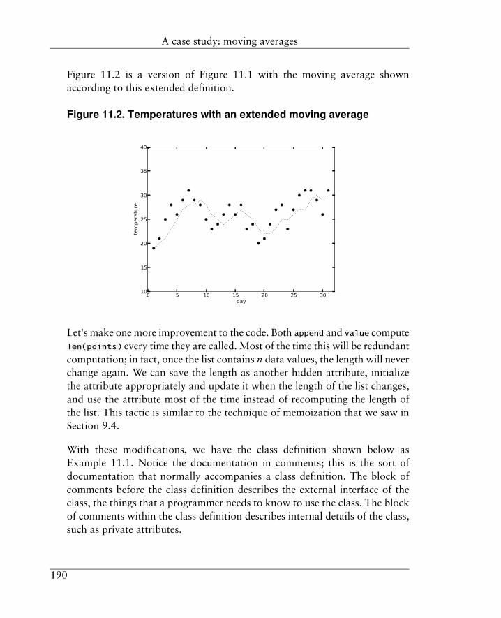
Figure 11.2 is a version of Figure 11.1 with the moving average shownaccording to this extended definition.

Figure 11.2. Temperatures with an extended moving average

Let's make one more improvement to the code. Both append and value computelen(points) every time they are called. Most of the time this will be redundantcomputation; in fact, once the list contains n data values, the length will neverchange again. We can save the length as another hidden attribute, initializethe attribute appropriately and update it when the length of the list changes,and use the attribute most of the time instead of recomputing the length ofthe list. This tactic is similar to the technique of memoization that we saw inSection 9.4.

With these modifications, we have the class definition shown below asExample 11.1. Notice the documentation in comments; this is the sort ofdocumentation that normally accompanies a class definition. The block ofcomments before the class definition describes the external interface of theclass, the things that a programmer needs to know to use the class. The blockof comments within the class definition describes internal details of the class,such as private attributes.

190


Example 11.1. The MovingAverage class# MovingAverage: a moving average of a sequence# of numbers.# MovingAverage(n) constructor, where n = number# of values to average over# append(self, a) append a to the sequence# value(self) average of the n most recently# appended values, or of all if# fewer than n; None if none


# private attributes:# _ _nPoints nunber of values to average over# _ _points list of at most that many values# _ _length length of _ _points, kept current

def _ _init_ _(self, nPoints):self._ _points = [ ]self._ _length = 0self._ _nPoints = nPoints

def append(self, newValue):points = self._ _pointsif self._ _length == self._ _nPoints:

points.pop(0)else:

self._ _length += 1points.append(newValue]

def value(self):points = self._ _pointslength = self._ _lengthif length > 0:


return None

So far so good. This implementation of Moving Average will be perfectly goodfor many purposes. But will it be efficient enough for all purposes? We mightbe able to tell if we know how the class will be used.

191


Suppose that in a particular program the value method is called much morefrequently than the append method. Perhaps the stream of data produces newvalues rather infrequently, as in the case of a weekly or monthly economicstatistic. But perhaps the code is part of a popular web site that receives manyrequests per second for the value of the moving average.

In a situation like this, the value method often recalculates the averageunnecessarily when the data values have not changed. We can eliminate thisredundant computation by calculating the average whenever append is calledand storing the value as another private attribute, which the value methodcan use when it is called. Again we are using memoization, and now value isimplemented by accessing data instead of by performing a computation.

With this modification, MovingAverage might be defined as shown below inExample 11.2. The new data attribute is _ _value; notice that it doesn't evenexist until self._ _length is greater than zero, but we never use its value untilthen.

Version 2 of MovingAverage is not necessarily better than the original versionin all situations. Suppose now that append is called much more frequently thanvalue. Perhaps the stream of data is a physical measurement from a jitterysensor and arrives thousands of times a second, but the value of the movingaverage is required only once a second or once a minute. Then append computesthe moving average many times when it is never used.

Thanks to object-oriented programming, though, the two versions ofMovingAverage are completely interchangeable in any program. The externalinterface to the class, as documented in the blocks of comments before theclass definition headers, is identical in the two versions. We can measure theefficiency of a program and substitute version 2 for the original version, orvice versa, to try to improve efficiency any time we like. No code that usesthe class, such as the code in the smooth function (p. 187), would need to bechanged in any way.

192


Example 11.2. The MovingAverage class, version 2# MovingAverage: a moving average of a sequence# of numbers.# MovingAverage(n) constructor, where n = number# of values to average over# append(self, a) append a to the sequence# value(self) average of the n most

recently appended values


# private attributes:# _ _nPoints number of values to average over# _ _points list of at most that many values# _ _length length of _ _points# _ _value average of values in _ _points# justification for memoizing _ _value: value() is# called much more frequently than append()

def _ _init_ _(self, nPoints):self._ _points = [ ]self._ _length = 0self._ _nPoints = nPoints

def append(self, newValue):points = self._ _pointsif self._ _length == self._ _nPoints:

points.pop(0)else:

self._ _length += 1points.append(newValue]self._ _value = sum(points) / self._ _length

def value(self):if self._ _length > 0:

return self._ _valueelse:

return None

193


11.6. Recursively-defined objects: treesIn the examples that we have seen so far, the values of the data attributes ofprogrammer-defined classes have been values of built-in Python types, butthey can also be objects that are instances of other programmer-defined classes.For example, consider the attribute address in the Person and Customer classesof Sections 11.2 and 11.3. The values of address were strings, but if we hadan Address class (perhaps having its own attributes such as street, city, andso on), the values of address could be Address objects instead (with appropriatechanges to the addressLabel methods, of course).

In fact, the value of an attribute can be an instance of the same class that isbeing defined. For example, suppose that we are defining a class Person. Twoof the attributes of a Person object might be the person's mother and father.The values of these attributes might themselves be Person objects.

Then the Person class is defined partly in terms of itself, much as a recursivefunction is. We say that an instance of this class is a recursively-defined object.Recursively-defined objects are important in computer science, and knowinghow to work with them is a useful programming skill.

Let's consider one kind of recursively-defined object: the tree. We saw treesbriefly in Section 6.6. There are a number of ways of describing trees inmathematics and computer science, and we'll look at several of them, includingrecursive descriptions.

In the study of graphs, a tree is a kind of graph. A tree can be either a directedor an undirected graph. We will concentrate on directed trees of a particularkind: those that have a distinguished vertex called the root from which pathsradiate. Trees of this kind can be defined by the following two properties:

• There is one and only one vertex with no edges leading to it. That vertexis the root of the tree.

• Each other vertex has one and only one edge leading to it.

194

Recursively-defined objects: trees

These properties imply that for every vertex in the tree, there is a path fromthe root to that vertex, and no more than one. Paths in a tree never converge.

If a tree is finite (and we will consider only finite trees), it must have leaves,which are vertices with no edges leading from them.

Here is an example of a tree. This one is unlabeled, and this time the root isat the top of the picture and the leaves are toward the bottom.

Now here is a recursive definition that defines trees of the same kind:

A tree is either

• a leaf, or

• a vertex (the root) with edges to one or more subtrees, which aretrees defined in the same way.

Let's look at variations on the recursive definition of a tree. Here is one:

A tree is either a leaf, or an object containing one or more subtrees,which are trees defined in the same way.

195


Here, instead of speaking of edges to the subtrees, we speak of the subtreesas being contained in the larger tree. The trees are nested, much as expressionsand compound statements in Python are nested.

This is the view that we often take in programming, especially whenprogramming with objects. Instead of a tree being a graph with edges, it is anobject that has other trees as attributes. The edges may actually be presentanyway, as bindings or pointers, depending on how the programmer or theprogramming language implements the tree objects. Sometimes we think ofthe edges explicitly when visualizing a tree or drawing a picture of it, but oftenwe don't.

Here is another definition that is slightly different:

A tree is either empty, or is an object containing one or more subtrees,which are trees defined in the same way.

With this definition, a leaf is a tree all of whose subtrees are empty.

This definition allows a tree to be nothing at all, which makes no sense inmany contexts. However, empty trees can be useful in programming, as wewill see.

In computer science work, vertices of a tree are often labeled; in fact, sometimesa vertex has more than one piece of data attached to it. If trees are programmedas objects, each vertex is represented by a tree object, and its attributes arethe labels and other data as well as the subtrees.

The data attached to different vertices can be of different kinds. Here is atypical example of a computer-science tree: it represents an expression.

196


The expression is “x + y*z”; perhaps it is part of a program. The leaves arelabeled with the names of variables, and the other vertices are labeled withoperators. Programming-language interpreters and compilers often use similartrees to represent expressions and other parts of programs.

Trees are ideal for representing nested structures like expressions. They arealso useful for representing information of many other kinds, includinghierarchy relationships. The tree below represents a hierarchy of classes andsubclasses like the one presented in Section 11.3. (This is an example of a treethat is not binary.)

In common English usage there are “trees” that are actually trees in themathematical sense, structures like those that we have been discussing. Theyare family trees.

197


There are two kinds of tree that are commonly called “family trees”: oneshows the ancestors of a given person, and the other shows the descendantsof a given person. We will consider the first kind, which we will call an“ancestry tree”.

Figure 11.3 shows an ancestry tree for a certain person named William. Inthis diagram older people are toward the top and younger people are towardthe bottom, so the root of the tree is at the bottom. The edges point from aperson to the person's father (up and toward the left) and mother (up andtoward the right). Of course, the tree does not show all of William's ancestry;there are people in the tree (the leaves of the tree) whose fathers and mothersare not represented in the tree.

Figure 11.3. An ancestry tree

Notice the subtrees, which are trees of the same kind as the larger tree. Forexample, the tree whose root is labeled “Charles” is an ancestry tree forCharles.

Now let's see how we might represent such a structure as a recursively-definedobject in a program.

198


Using Python as always, let's define a class called Person. Each instance of theclass will represent a person in an ancestry tree, and will have the attributesname, father, and mother. Here are the class heading and the constructor:

class Person:

def _ _init_ _(self, name, father, mother):self.name = nameself.father = fatherself.mother = mother

Then we can construct William's ancestry tree by using code like the following.We construct Person objects for parents first, so that we can use those objectsas values for the values of the father and mother attributes for younger people.We use the value None for the father and mother of people at the leaves of thetree; of course this means that the tree contains no information about theparents of these people, not that they have no parents!

george = Person("George", None, None)elizabeth = Person("Elizabeth", None, None)elizabeth2 = Person("Elizabeth", george, elizabeth)philip = Person("Philip", None, None)charles = Person("Charles", philip, elizabeth2)diana = Person("Diana", None, None)wiliam = Person("William", charles, diana)

This code is only for illustration. In practice, especially for a larger tree, wewould probably want to get the data from a file rather than hard-coding itinto the program (see Exercise 4).

Now, once we have a tree or other recursively-defined object, how can weprocess it? Here is a very important principle:

A computation that processes a recursively-defined data object is likelyto be recursive itself, with its structure following the recursive definitionof the object.

For example, here, in broad outline, is the structure of many computationsthat process trees:

199


To process a tree:if it is a leaf:

do something with the data in the leafelse:

do something, possibly different, with the data in the rootand recursively process each of the subtreesand combine the results

Not all computations on trees can be made to fit this pattern. But if acomputation can, it is likely to be simpler and more obviously correct than acomputation that does the same job in some other way.

Here's an example. Let's write a method for the Person class to construct aset of the names in the ancestry tree of a person.

We'll follow the above recursive pattern. Whether or not the Person is a leaf,we'll start by taking the name of the person, as a one-element set. Then, if theperson's father is represented in the tree, we add the names in the ancestrytree of the father, and similarly for the person's mother. Notice that the “+”in the augmented assignment operator “+=” is set union.

def ancestorNames(self):result = { self.name }if self.father != None:

result += ancestorNames(self.father)if self.mother != None:

result += ancestorNames(self.mother)return result

This solution is not bad, but we can simplify it. Consider the recursivedefinition of a tree that allows a tree to be empty. It makes no sense for anancestry tree for a person to be empty — it always includes the person at least— but suppose we let the father or mother attribute of a Person object be anempty tree? Then a value of None, instead of being a marker that indicatesmissing information, represents an empty subtree.

Now, instead of having to test each subtree for the None value, we simply letthe empty tree be the basis case for the recursion. The set of names in an empty

200


ancestry tree is the empty set, of course. Following this line of reasoning, wearrive at the following solution:

def ancestorNames(self):if self == None:

return set() # the empty setelse:

return { self.name } \+ ancestorNames(self.father) \+ ancestorNames(self.mother)

This code is not only simpler, but more closely follows the pattern of code fora recursive function definition that we have often seen, going back to thefactorial function of Section 4.2. The basis case and the recursive case areclearly separated, so that it is easier to see at a glance that the method bodycomputes what we want.

This example illustrates two principles:

1. It's fine to choose a mathematical definition that makes your programmingjob easier, or to tweak a definition to your advantage.

2. Don't tweak the code and ignore the mathematical definition! Pick adefinition, make sure that it says what you want, and then write the codeto match the definition.

11.7. State machinesThe state of an object is information that the object retains from one methodcall to another. A method may cause the object to change state (as the appendmethod of a MovingAverage object does), and the result of a method call maydepend on the object's state (as in the case of the value method).

In designing objects in programs, it is sometimes useful to think explicitly ofstates and transitions between states. This is especially true when the numberof possible states of an object is finite and rather small. Then we can give eachstate a name.

201

State machines

Furthermore, we can show the behavior of the object by drawing a transitiondiagram. This is a particular kind of a labeled directed graph, in which eachvertex is labeled with the name of a state and each edge is labeled with thename of a stimulus or input that causes a transition from one state (at the tailof the edge) to another (at the head).

A transition diagram defines a state machine, which in computer science theoryis a kind of mathematical object. Most mathematical properties of statemachines are beyond the scope of this book, but we'll simply use state machinesand their transition diagrams to help us describe and design objects. Softwaredesigners often do this, and so do other professionals such as hardwaredesigners.

For example, consider the kind of electrical pushbutton that you click onceto turn on and click again to turn off. We can describe it as a state machinehaving two states, off and on, and a single stimulus called “click” that causesa transition from each state to the other. Here is the transition diagram forthat state machine:

Now consider a slightly more complicated kind of elecrical device. When youclick it, it works like the previous kind of pushbutton. But there's no way of

202

State machines

looking at the button to tell whether it is on or off, so the manufacturer hasadded a “reset” capability: when you press and hold the button down forseveral seconds, it turns off, whether it was on or off before. Here's thetransition diagram for the corresponding state machine:

We can define a Python class whose objects behave like this device does, andwe can use the transition diagram as a guide as we write the code. The stateof the object will be stored in a private data attribute. There are only twostates, so the attribute needs to have only two possible values. Boolean valuesare one obvious choice: we name the attribute _ _on, and we use the valueTrue to represent the state on and False to represent the state off.

The _ _init_ _ method sets the _ _on attribute to an initial value; we arbitrarilychoose False. The effect of the “click” stimulus is implemented by a methodwith that name. It sets the value of _ _on to True if it was False and False ifit was True; we could use an if-statement to do this logic, but the Boolean not

operator does the same thing more easily. The “reset” stimulus is handled byanother method, which simply sets _ _on to False. The method isOn returnsthe value of the attribute as a Boolean value. All this code is very simple; it isshown as Example 11.3.

Now let's look at an example of a state machine object that does a typicalkind of programming job: finding fields in a string. Perhaps the string is a linefrom a flat file, as in Section 8.4, but in the current example the fields areseparated by sequences of one or more space characters, rather than by commasas in a CSV file; there may also be spaces at the beginning and end of thestring. A field may contain any character that is not a space. We want todeliver the fields of a string as a sequence, perhaps as a stream.

203

State machines

Example 11.3. The Pushbutton classclass Pushbutton:

def _ _init_ _(self):self._ _on = False

def click(self):self._ _on = not self._ _on

def reset(self):self._ _on = False

def isOn(self):return self._ _on

There are a number of ways of doing the job, but we'll show how to do itwith the aid of a state machine. Here's the concept: the state machine willreceive one character at a time from the string as a stimulus, and keep trackof whether the currect character is within a field or within a sequence of spaces;those will be the two states of the machine. The state matters, because acharacter can mean different things depending on its context; for example, aspace coming after other spaces means nothing and can be ignored, but aspace coming after non-space characters signals the end of a field.

The notation of transition diagrams has a number of variations, and we'll usetwo of them in this example:

• An arrow pointing from outside the graph to one of the states, denotingthe initial state of the machine; that is, the state that the machine starts inwhen it is created or turned on.

• An additional label on each transition, which is the name of a response toa stimulus. For example, a stimulus may be an input to a device, and theresponse would be the corresponding output. The response is what themachine does when it is in a particular state and receives a particularstimulus.

204

State machines

In our state machine, the stimuli will be characters from the string that we aretaking apart, and the responses will be the “meaning” of each character inthe context of the characters that have come before it. The different responsesthat we will need are:

• “include”: the character is part of a field.

• “ignore”: the character means nothing and can be ignored.

• “end”: the character signals the end of a field, but is not part of the field.

Here is the transition diagram for the state machine. The two states are labeled“in spaces” and “in field”. Since the string may start with spaces, the initialstate is “in spaces”. In this state, a stimulus of a space character sends themachine back to the same state, and the response is “ignore”. Any othercharacter is the first character of a field, so the machine goes to the state “infield” and the response is “include”. (You can think of the annotation “non-space” as indicating that this edge in the graph is a shorthand for many edges,one for each possible character that is not a space.) In the state “in field”, anycharacter but a space sends the machine back to the same state, with theresponse “include”. A space signals the end of the field, so the machine goesback to the state “in spaces” and the response is “end”.

Now we can translate this transition diagram to Python code. There's onedata representation decision to make: how will we represent the different

205

State machines

states of the machine and the different responses? Both collections are sets:they have no particular order and all elements are different. But it turns outthat we won't need to do any set operations on these sets; we will only needto compare two values for equality. In a situation like this, we can simplyrepresent every element of each set as a small integer value, as we noted inSection 8.5.

inField = 0inSpaces = 1

include = 0end = 1ignore = 2

And now we write a class definition for the state machine that we want; thecode is Example 11.4. The state of the machine is the data attribute self.state,and the constructor sets it to the initial state. We provide a method advance

that takes a character as a stimulus and performs one state transition, settingthe new state and the response depending on the old state and the character.We return the response as the value of the method call.

Example 11.4. A state machine for finding fields in a stringclass FieldsStateMachine:

def _ _init_ _(self):self.state = inSpaces

def advance(self, char):if self.state == inField:

if char == " ":self.state, response = inSpaces, end

else:self.state, response = inField, include

else: # self.state == inSpacesif char == " ":

self.state, response = inSpaces, ignoreelse:

self.state, response = inField, includereturn response

206

State machines

The code that uses the state machine is shown as Example 11.5. We define agenerator function that yields fields of a string one at a time. We feed eachcharacter of the string to the state machine. We accumulate the characters ofa field in the variable field, appending a character to it if the machine'sresponse to the character is “include”. If the response is “end”, we yield thefield and start a new one. When we reach the end of the string, the last fieldmay not have been ended by a space at the end of the line; in this case, weyield that last field.

Example 11.5. Code that uses a FieldsStateMachinemachine = FieldsStateMachine()

def fields(string):field = ""

for c in string:response = machine.advance(c)if response == include:

field += celif response == end:

yield fieldfield = ""

# else response == ignore: pass

if field != "":yield field

So far so good. But this example is very simple, and the code doesn't doanything we couldn't do more easily in other ways, such as with the Pythonsplit method. Now let's add a complication or, as we say in the softwareworld, a “feature”.

Suppose that a field in the input file is allowed to contain spaces. Perhaps afield is the name of a city, so that cases like “Los Angeles” and “East St. Louis”must be allowed. Then when a field may contain a space, it is enclosed indouble-quote characters, like this: "East St. Louis". The double-quotecharacters are not considered part of the data that the field represents.

207

State machines

Now our state machine must contain a new state and some new transitions.In the state in spaces, a double-quote character causes a transition to the newstate in quoted, meaning inside a quoted field; the double-quote character isignored. The machine stays in that state until a double-quote character isreceived, which ends the field. The new state transition diagram is shownbelow; “quote” means a double-quote character.

The revised code for the state machine is shown as Example 11.6. The changesare easy to make, once we have the new transition diagram: we just need toadd code for the new state and the new transitions. The body of advance maylook long and complex, but its structure is quite regular, and we can easilycompare the various parts to the corresponding parts of the transition diagramto make sure that we have written the code correctly.

By the way, computer scientists have observed that a monoid can be definedfrom transitions in a state machine, and computer science theory develops theimplications of this fact. Those results are not immediately relevant in day-to-day programming, though, so we won't present the details here. Let's just usethe observation to reinforce the idea that, in computing, monoids areeverywhere.

208

State machines

Example 11.6. A state machine for finding fields, version 2inField = 0inSpaces = 1inQuoted = 2

include = 0end = 1ignore = 2

class FieldsStateMachine:

def _ _init_ _(self):self.state = inSpaces

def advance(self, char):if self.state == inField:

if char == " ":self.state, response = inSpaces, end


elif self.state == inQuoted:if char == '"':

self.state, response = inSpaces, endelse:

self.state, response = inQuoted, includeelse: # self.state == inSpaces

if char == " ":self.state, response = inSpaces, ignore

elif char == '"':self.state, response = inQuoted, ignore


return response

Terms introduced in this chaptersuperclassattributes of an objectoverriding a methodstate of an objectprivate attributeclassrecursively-defined objectidentity of an objectrootinstance

209


leafconstructorsubtreename spacestate machineinheritancetransition diagramsubclass

Exercises1. Write a Python class Multiset that is based on dictionaries. The class

must implement the methods isEmpty, count, intersection, union, andsum.

In Python a programmer-defined class can inherit from a built-in class,so you might try making your Multiset class inherit from the dict class.What are the advantages and disadvantages of doing so?

2. Write a Python class Monoid. Give it at least the following methods:

• An _ _init_ _ method that takes two arguments, a two-argumentfunction that implements the monoid operation and a value for themonoid identity. For example, here's how the class constructor mightbe called:

integerAddition = Monoid(lambda x,y: x+y, 0)

• A method apply that takes two parameters, applies the monoidoperation (the function that was the first argument to the constructor)to them, and returns the result.

• A method reduce that takes an iterable of values as a parameter andreduces its elements to a single value, using the monoid operation andthe monoid identity, much as the reduce method of Section 6.4 does.

3. Write a variant of the MovingAverage class that is suitable for data that isnot equally-spaced in time. The argument to the constructor, instead ofbeing a number of data points, will be a duration (in appropriate units,such as seconds or days) over which the moving average is to be computed.

210

Exercises

The argument to the method append will be an ordered pair of a time (inthe same units) and a data value that corresponds to that time.

4. Design the structure of a file that a program could read to build an ancestrytree of the kind we saw in Section 11.6. Be aware that in an ancestry treeit is not too uncommon for two or more people to have the same name;a name does not uniquely identify a person in the tree.

Write a method for the Person class to read a file with this structure.

5. a. Write a method ancestors for the Person class that constructs the setof all ancestors of a person (including the person), not just the set ofancestors' names. Perhaps there are several people with the same namebut differing in other attributes that we haven't mentioned so far, suchas birth and death dates; you want to include everyone who is anancestor.

b. Now how can you find the set of ancestors of a given person, notcounting that person? No, don't try to write a method that makes theoriginal person a special case! Do it an easier way.

c. Using your ancestors method, how can you construct the set ofancestors' names? Do it with a single Python expression.

6. Add attributes born and died to the Person objects of Section 11.6; theirvalues will be integers, representing the years in which the person wasborn and died. Use None for the value of died for a person who is stillalive.

Write a method that takes self and a year as arguments, and returns theset of ancestors of a person (including the person) who were alive duringthe given year.

7. Modify the Person class of Section 11.6 so that it can be used to constructa tree of descendants of a person. Then a Person object will have attributesthat are the children of the person rather than the parents. How will yourepresent the collection of children of a person?

211

Exercises

Write a method for this class that constructs the set of descendants of aperson, including the person.

8. Modify the fieldsStateMachine class of Section 11.7 to add one morefeature: a quoted field may now contain a double-quote character as partof the data that the field represents. The two-character sequence “\"”now represents a double-quote character within the field. Also, so that aquoted field can still contain a “\” character as part of the data that thefield represents, the two-character sequence “\\” now represents a single“\” character within the field. In fact, to simplify things, let's say that a“\” character followed by any character represents the second character.Draw the new state transition diagram, and then write the correspondingcode.

9. Design the structure of a file to encode the kinds of transition diagramsshown in Section 11.7: the states, initial state, stimuli, responses, andtransitions. Now write a program that will read such a file and produceas output an advance method like the one in Example 11.6.

Such “code-generating” programs are used by writers of programming-language interpreters and compilers to help produce code for such jobsas finding the names, keywords, constants, operators and punctuationmarks in lines of programs.

212

Exercises

Chapter 12Larger programs12.1. Sharing tune lists

In this chapter we'll examine how we might apply the ideas presented in thisbook to larger programming problems. We won't present whole programs —they would take too much space in the book and would be tedious to read intheir entirety anyway — but we'll sketch how the programs might be designedand, especially, how mathematical structures might be used in the designs.

Here's our first case study. The task is to build a program to make it easy forfriends to share lists of their favorite tunes from those that they play on theircomputers and mobile devices.

The program will allow people to send recommendations to their friends, asyou would expect, but it will also keep track of the songs that a person plays.It will send lists of the tunes that the person has played most often, perhapsonce a week, to all of the person's friends through the wireless connectionson their devices. It will also receive tune lists from the friends and compilethem into a single list arranged by popularity. People can use these tune listsas recommendations, and look up the tunes in their own tune libraries, or (forexample) look for other tunes by the same artists.

That's the statement of the problem in brief. Now let's see how we mightdesign the program. We'll show some fragments of the actual Python codetoo.

A “tune list” is a sequence, in order by some measure of popularity, but notnecessarily a list in the Python sense. Each tune has a number of attributes:artist, title, composer, perhaps genre, and so on. Our program will processthe attributes of tunes, not the sound files themselves. A tune is identified byits collection of attributes. If all the tunes came from one source, such as aparticular company's online music store, we could use something like the

213

catalog number in the store to identify a tune, but we assume that the tunescan come from a number of different sources, including home recording.

We'll represent a tune by a Python tuple, in which the first element is the artist,the second element is the title, and so on for as many attributes as we wantto include. Other representations are possible (see the exercises at the end ofthe chapter), but the tuple representation will lead to a simple design. A tupleis an immutable object, so we can form sets of them and use them as dictionarykeys. Let's call each of these tuples a “tune-tuple”.

Each attribute will be at a fixed position in every tune-tuple. To accessattributes by name, we define a set of functions that map a tune to one of itsattributes:

def artist(tune):return tune[0]

def title(tune):return tune[1]

and so on for all the attributes that we want to access by name.

A person's tune library will be represented by a set of tune-tuples, forming arelation if we want to think of it that way. The data will come from a file thatis in a variant of CSV format: each line represents a tune and contains itsattributes separated by vertical-bar characters (“|”). This format allowsattributes such as tune titles to contain commas, which is not too uncommon.We can build the set of tune-tuples using a variant of the setOfTuples functionfrom Section 8.4. Here is the definition we use; we simply split on vertical-barcharacters instead of commas. Notice the set comprehension.

def setOfTuples(fileName):file = open(fileName)return { tuple(line.strip().split("|"))

for line in file }

Then if the data file is named “myTunes”, we do this to build the set-of-tuplesstructure:

myTunes = setOfTuples("myTunes")

214

Sharing tune lists

As a person plays tunes, the tunes are communicated to our program (bymeans that are beyond the scope of this book) as a stream of tune-tuples. Ourprogram accumulates the tune-tuples in a multiset. We use a multiset, not aset, because of course the person can play the same tune more than once, andone of our goals is to count how often each tune is played.

We define a class of multisets, since (as you'll see) we'll need several of them.We implement a multiset as a mapping from values to counts, using adictionary as we did in Section 9.5; we keep the dictionary in a private dataattribute. We provide a tally method like the function of that name that wedefined in Section 9.5.

class Multiset:

def _ _init_ _(self):self._ _count = {}

def tally(self, value):if value in self._ _count:

self._ _count[value] += 1else:

self._ _count[value] = 1

We create a Multiset object named plays, and as a person plays tunes, thetune-tuples are entered into it:

plays.tally(tune)

In the class Multiset, we provide another method to extract a tune list fromthe plays multiset. The method is called topN, and returns the n tunes withthe most plays, highest first. Here n is an argument, to let the user set thenumber as a preference; there is nothing magical about the number ten. Inany case, to get a play list of the top 10 tunes, we would write something likethis:

playList = plays.topN(10)

There are several ways that topN could produce the required list. Here are twoof them:

215

Sharing tune lists

1. Produce the contents of _ _count as a sequence of ordered pairs in whichthe count comes first and the tune tuple comes second:

byCount = ( (count, tune)for (tune, count) in items(self._ _count) )

Sort that sequence using the builtin function sorted, which produces a listin ascending order of count (and, within subsequences of equal count, inascending order of tune-tuple, but that's not so important). Reverse theresult (the Python library has a list method reverse), take a slice of the firstn elements of the resulting sequence, and produce a sequence of just thetune-tuples from the ordered pairs using a comprehension.

2. The builtin function sorted can, with extra arguments, do most of the workand produce a list sorted by count in reverse order in one step. This methodrequires some Python that we haven't covered in this book, but if you'reinterested you can look in the Python documentation for the function sorted

and the phrase “keyword argument”.

However topN does it, we get a sequence of the tunes that the user has playedmost often, and we transmit the sequence to each of the user's friends in thesame CSV form that we use for the user's tune library. (As with the stream ofthe user's plays, we won't discuss how the program sends or receives tunelists.) The collection of friends is a set: perhaps a set of online addresses, or aset of objects each having a person's online address as an attribute.

Meanwhile, the program receives (we won't discuss how) tune lists andrecommendations from the friends. A recommendation is a tune-tuple and amessage (probably a comment about the tune) in some suitable format; theprogram represents the recommendation as an ordered pair of a tune-tupleand a string. The program collects the tune lists in a set called friendsLists

and the recommendations in another set called friendsRecommendations.

The program will be able to display all the tune lists and recommendations,but the program will also be able to tabulate both and produce aggregatedtune lists. Like the user's plays, these are multisets at first and are thenconverted into sorted sequences. Unfortunately, we can't write multisetcomprehensions in Python, but we can still construct the multisets easily using

216

Sharing tune lists

for-statements and tally. For example, to produce a list of the tunes with theten highest number of mentions in the tune lists of the friends, here's how thecode might look:

allMentions = Multiset()for fList in friendsLists:

for tune in fList:allMentions.tally(tune)

topTenMentions = allMentions.topN(10)

Or to produce a list of the ten tunes that are first in the greatest number oftune lists of the friends:

allMostPopular = Multiset()for fList in friendsLists:

allMostPopular.tally(fList[0])topTenMostPopular = allMostPopular.topN(10)

Or to produce a list of the ten tunes recommended by the most friends (recallthat the first element of a recommendation pair is the tune-tuple):

allRecommended = Multiset()for rec in recommendations:

allRecommended.tally(rec[0])topTenRecommended = allRecommended.topN(10)

We could also produce an aggregated tune list of the tunes played most oftenby the friends, weighed by the number of plays of each tune. For thiscomputation we would need the counts, of course, so we would have eachfriend's machine transmit pairs of tunes and their counts, pruned to the topten or some such number, rather than just a tune list; in other words, anothermultiset. Then we could produce an aggregated tune list by doing a big multisetsum or union of all the multisets coming from the friends. We might or mightnot find such a list useful, because it would be heavily weighted toward thetastes of the friends who spent most time listening to tunes, but it might bean option worth considering.

Then the user might want to play the tunes on any of these aggregated lists,or to search for tunes like them. Code to determine whether a given tune isin the user's tune library would simply contain the Boolean expression

217

Sharing tune lists

t in myTunes

Perhaps the user would like to see tunes in the tune library that have the sameartist as a given tune. We could get the set of such tunes with a comprehension:

{ t for t in myTunesif t.artist() == tune.artist() }

Notice that this is a relational selection operation (Section 10.5). You canprobably think of similar computations that the program might do.

Now let's review the mathematical structures that this case study has used:multisets, certainly, but also sets and set comprehensions; n-tuples; sequencesof various kinds; mappings such as artist, title, and topN; and relations. Ineach case, notice how the mathematical structure was a natural choice for thejob to be done.

12.2. Biological surveysOur next case study is a program to record data from biological surveys.

For our purposes, a biological survey is a count of organisms of different kindsin a particular place or at a particular time or both. One good example is theChristmas Bird Count in North America. Other examples might be a countof grasses and wildflowers in a meadow, or a count of fish passing a particulardam over some period of time.

Usually a participant in a biological survey records different kinds of organismsobserved and how many of each, and our program will accumulate thesecounts. Sometimes, as perhaps in the case of grass plants in a meadow, aparticipant may not count individuals, but our program will still be able tocount the number of participants that observed a particular kind of plant. Orthe meadow might be divided into grid squares, and the program would countthe number of squares in which an organism was observed. In any case, theprogram will accumulate counts, like the tune-list program in Section 12.1does. But this time we won't represent the data explicitly as a multiset — thatis, as a set of key-and-count pairs — because another structure for the datais more important, as we will see.

218

Biological surveys

In biology, a “kind” of organism is called a “taxon” (plural “taxa”). A taxonis identified by a scientific name, usually derived from Latin, and it often hasa common name in English or whatever the local modern language may be.Taxa are arranged into levels called “ranks”, from more general to morespecific. For example, for birds the major ranks are as follows (scientific namesare shown in italics):

• Class. Example: Aves (birds).

• Order. Example: Strigiformes (owls).

• Family. Example: Strigidae (typical owls, not barn owls).

• Genus. Example: Bubo (horned owls).

• Species. Example: Bubo virginianus (Great Horned Owl).

Often, as in the case of birds, there are also intermediate ranks such assuperorders and subfamilies. Our program will not have a particular set ofranks built in, but will use whatever ranks are in the data that we are given.

Each taxon except those at the lowest rank, then, comprises one or more taxafrom the next rank down. The class Aves, for example, comprises theStrigiformes, the Gaviiformes (loons), the Sphenisciformes (penguins), andtwo dozen or so more orders.

Our program will need to represent this hierarchical structure of taxa, becausea survey participant doesn't always identify a specimen down to the speciesrank (“It was a hawk, but I couldn't tell what kind”). In some surveys (ofinsects, for example), identification of many specimens down to the specieslevel is probably too hard for many survey participants, and we would expectthat most of the counts would be of taxa above the species rank. In any case,the program must be prepared to keep counts of taxa at any rank.

Now let's sketch the design of the program. The central structure is a Taxon

class having the following attributes:

• A scientific name, scientific.

219

Biological surveys

• A common name (optional), common.

• A rank, rank.

• A count, count.

• The taxon at the next rank up which contains the current taxon, super. Itmay be None, which happens when the program doesn't keep data for thetaxon that would be at the next rank up. This would be the case for Avesin a survey of birds, for example. In any case, no taxon is contained in morethan one higher-rank taxon.

• A set of subordinate taxa at the next rank down, sub. We assume that forour purposes the ordering is not important.

A Taxon with its sub set is a recursively-defined object, like the ancestry treesof Section 11.6, and so is the root of a tree. We don't require that all the Taxonobjects be contained in one big tree with a single root; for example, in thesurvey of the meadow, there may be one tree containing all the grasses andanother containing all the wildflowers. But each taxon is the root of some treeor subtree.

With the super attribute, the Taxon objects form a more complex recursively-defined structure. Recall from Section 11.6 that we can picture a tree as adirected graph; in a recursively-defined tree, an edge represents a binding orpointer from an object to another object which is an attribute of the first.

220

Biological surveys

The super attribute adds edges in the opposite direction. Now we can thinkof the whole structure as a directed graph that is not a tree, but perhaps it ismore useful to think of it as an undirected tree. The sub edges and super edgesare paired, and each pair is like a single undirected edge that you can use togo in either direction.

We get the structure of the taxa from a data file, in CSV form as usual. Eachline is a tuple defining a Taxon object and has the following fields:

• A scientific name, defining the scientific attribute.

• A common name, possibly empty, defining common.

• A rank, defining rank.

• The scientific name of the taxon at the next higher rank of which this taxonis a part, possibly empty, defining super.

The file line does not need to define the sub attribute, because it can be derivedfrom the super attributes of the other Taxon objects.

For example, the line for Bubo might look like this:

Bubo,horned owl,genus,Strigidae

The taxa file is ordered by rank, highest first, so we can assume that the linefor Strigidae (for example) comes before the line for Bubo. Other than thisconstraint, the lines of the file are unordered. But since the lines are not

221

Biological surveys

completely unordered, the file does not quite represent a relation in themathematical sense. (It happens to be an example of another kind ofmathematical structure called a “partially ordered set”, which we haven'tdiscussed in this book.)

The constructor of the Taxon class in the code (let's be careful not to confusePython classes with biological classes!) is called with the fields of a file line asarguments, and the _ _init_ _ method fills in the scientific, common, andrank attributes, and initializes count to zero. If the super parameter is notNull, _ _init_ _ must also find the Taxon object with that name, set self.superto that object, and insert the current object into the sub set of that object. Buthow do we find the object?

Let's keep a dictionary taxon that maps scientific names to Taxon objects; the_ _init_ _ method inserts an entry into it for the newly-created Taxon object.We keep a similar dictionary taxonByCommon that maps common names toTaxon objects; we'll see a use for it later.

Because of the ordering of the taxa file, when _ _init_ _ is called the Taxon

object for super already exists and taxon already contains the correspondingentry. (Throughout this case study, we won't show code that would deal witherrors in the data, such as lines in the taxa file being in the wrong order ormissing.) For the current Taxon object, we initialize the sub attribute to theempty set; it will be filled in as later lines of the taxa file are processed.

So here's what we have so far:

222

Biological surveys

taxon = {}taxonByCommon = {}

class Taxon:

def _ _init_ _(self, scientific, common, rank, super):self.scientific = scientificself.common = commonself.rank = rankself.count = 0self.sub = set()

if super != "":superObject = taxon[super]self.super = superObjectsuperObject.sub.add(self)

else:self.super = None

taxon[scientific] = selfif common != "":

taxonByCommon[common] = self

We give the Taxon class an obvious method to add a number to its count whena survey participant reports some data:

def add(self, n):self.count += n

So when a survey participant reports a count of some taxon, we use taxon ortaxonByCommon (depending on which kind of name the participant has givenus) to find the corresponding Taxon object, and apply add to that.

Now we come to the method that all this other structure and code is designedto support. The method computes the total count observed for some taxon,including the count stored for the taxon itself and the counts of all subordinatetaxa all the way down the hierarchy. The computation, not surprisingly, isrecursive. We add the count attribute of the taxon to the sum of the totals ofall the elements of sub, and those totals are computed recursively in the sameway. It's all very simple:

def total(self):return self.count + \

sum((t.total() for t in self.sub))

223

Biological surveys

Notice that this recursion is not explicitly defined by cases. The basis case ofthe recursion is reached at the lowest level of the taxon hierarchy, whenself.sub is empty and so there are no recursive calls.

In the method, sum is a function that returns the sum of a sequence of numbers.Here is one possible definition of it, similar to the definition in Section 6.4(where we also defined reduce):

def sum(seq):return reduce((lambda x,y: x+y), seq, 0)

Now we can produce a report of the counts of a given taxon and all itssubordinate taxa, all the way down the hierarchy. For example, after a shorttime into a survey of birds, a report for the order Strigiformes might look likethis:

8 Strigiformes (owl)7 Strigidae (typical owl)2 Asio (eared owl)1 Asio otus (Long-eared Owl)1 Asio flammeus (Short-eared Owl)

0 Athene ()0 Athene cunicularia (Burrowing Owl)

5 Bubo (horned owl)5 Bubo virginianus (Great Horned Owl)

1 Tytonidae (barn owl)1 Tyto (barn owl)1 Tyto Alba (Common Barn Owl)

Here's a recursive Taxon method to produce such a report; the method producesa line for a taxon and then recursively produces a report for each subordinatetaxon. Notice how the parameter indent is used to cause the lines for taxa ateach lower level of rank to be indented two spaces further. Again, the recursionterminates when self.sub is empty.

def report(self, indent):print(indent + self.total() \

+ " " + self.scientific+ " (" + self.common + "))

for sub in self.sub:sub.report(indent + " ")

224

Biological surveys

Now notice that once the program has read the whole taxa file, values(taxon)is the set of all the Taxon objects for all the taxa that the program has dataabout (see Section 9.2). It is actually a stream, but in no particular order, sowe can think of it as a set. We can iterate over it, filter it, perform acomputation on each element, materialize it as a set, and so on.

Here's one possible use for values(taxon). In the taxa file for a survey, perhapsthe data defines one big tree with a single root, as it might in a bird survey(the root would be the Taxon object for Aves). But perhaps it doesn't. In thatcase, it defines a set of trees (not surprisingly, the mathematical name for sucha structure is “forest”).

We can get the set of roots of all these trees with a simple comprehension:

allTrees = { order in values(taxon)if order.super == None }

And then we can produce a comprehensive report of all the taxa counted,organized into the trees to which they belong:

for t in allTrees:t.report("")

As with the tune-list program in the previous section, you can probably thinkof other useful computations that we could add to the program.

Now suppose you were hired to write a program like this one. You completethe program using the design ideas above and submit it for approval. To yoursurprise, your boss asks for changes: there are a couple of additionalrequirements.

First, it seems that the taxa subordinate to a higher-rank taxon really do havean official ordering, called “taxonomic sequence”. The output produced bythe report method, as the Taxon class is currently defined, would not beacceptable to a biologist; the lines need to be in taxonomic sequence.

Second, some taxa have more than one common name. For one thing, namesof taxa change over time, and some survey participants might not know themost recent name for a taxon, or might be using old field guides containing

225

Biological surveys

some old names. For another, a survey may want to treat two or more commonnames as equivalent for counting purposes, such as “Snow Goose” and “BlueGoose” (they are the same species, but the Blue Goose is a “color morph” ofthe Snow Goose).

The boss says, “Sorry that I didn't think of these details before, but you'llneed to revise the program.”

Fortunately the changes are very simple. To meet the first new requirement,we use a list instead of a set for the container for subordinate taxa in a Taxon

object. We change only two lines in the constructor. Here they are:

self.sub = set()and

superObject.sub.add(self)

We change those lines to these:

self.sub = []and

superObject.sub.append(self)

Then we simply require that lines in the taxa file be in taxonomic sequence.Then the Taxon objects are created in taxonomic sequence, and the objects areappended to the appropriate sub lists in taxonomic sequence.

Now, for example, the report method produces its output lines in taxonomicsequence as well. The for-statement in the method's body does not need to bechanged at all, but now it iterates over a list rather than a set, and the list isin taxonomic sequence.

To meet the second new requirement, we use another data file that maps anyadditional common names to scientific names; it will be a CSV file as usual,and let's assume it is named synonyms. We will take each line of the file, convertit to a tuple using the setOfTuples function from Section 8.4, look up thescientific name in taxon to find the corresponding Taxon object, and add anentry to taxonByCommon for the new common name. The code is very simpleand the iteration has a familiar look:

226

Biological surveys

for (common, scientific) in streamOfTuples("synonyms"):t = taxon[scientific]taxonByCommon[common] = t

Only the official common name is stored in the Taxon object, but since allsynonymous common names map to the same Taxon object in thetaxonByCommon dictionary, they all contribute to the count of a single taxon.The boss is satisfied with this solution.

In this case study the central mathematical structure in the design is thestructure of the taxa, which at its heart is a tree or (in the general case) a setof trees. The structure is made of recursively-defined objects. With the super

attributes, the taxa structure is a directed graph, but we can also view it as anundirected tree. Mappings are also important in the design, especially taxon

and taxonByCommon, the recursively-defined mapping total, and the filesynonyms. The program also uses sets, as well as tuples and sequences of tuples.

12.3. Note cards for writersOur last case study will be a program to help writers manage fragments oftexts, such as outlines, notes, pieces of drafts and finished work, and citations.The program is designed for students writing papers and theses, and foracademic and professional writers writing articles and perhaps even books.

The program will be based on the metaphor of a note card, of the kind thatstudents and writers have traditionally used in their research. The programwill show “cards” as windows on a computer screen:

227

Note cards for writers

We join the software development project near its beginning. The organizationdeveloping the program has not completely decided on exactly what featuresthe program will have or how the program will work, but has ideas. Here aresome of them.

A user of the program will be able to create links among note cards, muchlike links among web pages. In fact, links will be able to point to several otherkinds of things, such as:

• Web pages.

• Digital documents, in formats like PDF and Postscript, and specific placesin documents.

• Entries in bibliographic databases.

A user will be able to annotate a note card with one or more keywords, andalso with one or more key-value pairs. For example, in the illustration below,the note card has two keywords and one key-value pair. In the latter, the valueis a link, perhaps to an entry in a bibliographic database.

A user will be able to search for cards with particular keywords, or cards withparticular values associated with particular keys. The program will also letthe user perform other kinds of searches, such as for cards containing particulartext.

Some keywords will be used to categorize cards as to their role, such as“outline” or “synopsis” or “draft”. Certain operations will most commonly

228


be done on cards having the same role; some such operations are splitting onecard into two or more shorter cards, combining two or more cards into onelonger card, and defining an ordering among cards.

As a user works on a document, ordering fragments of text and combiningthem will become more and more important. The ultimate goal, after all, isto create a document as a single long sequence of text, probably from thecontents of note cards having roles like “draft” or “final”. But as the work isin progress, the user might want to view the current state of all or part of thedocument by looking at a current outline or synopsis or draft taken from someor all of the note cards.

For example, consider the cards having the role “outline”. Suppose that onenote card represents the top-level of an outline of a document, and supposethat the card contains links to other cards representing more detailed outlinesof parts of the document. Those cards might contain links to other cards ofthe same kind, and so on. Then all these cards and links might form a tree:

A user might like to form one overall outline from this tree. Such an operationwould produce an indented outline like the bird-survey report of Section 12.2,and could easily be programmed recursively, like the report method in thatsection.

229


But what if the links form a directed graph that is not a tree — that is, if thereare note cards pointed to by more than one link?

What should the program do with cards like the one in the lower right? Shouldthe program include its contents the first time it finds the card as it traversesthe directed graph, or after it has processed all cards pointing to it? Or shouldthe program include its contents more than once? And what should theprogram do if the user has somehow created a cycle in the directed graph?These are some of the design issues that the developers of the program arestill debating.

In some situations the best solution may be to leave the ordering task to theuser. For example, the program might display cards as if they were spread outon a table top, and let the user move them around using the program'sgraphical user interface.

230


This interaction may also be what the program does when the user performsa search: the program may take the set of cards satisfying the search criterionand display them as if on a table top, and let the user order them or performother operations on them.

The developers of the program clearly have much more work to do and manymore decisions to make, but let's take the description of the program as itstands and describe it in terms of discrete-mathematical structures.

We can describe a note card as a 4-tuple having the following components:

• A title, which is a sequence of characters.

• A body, which is text that may contain links.

• A set of keywords, possibly empty. Each keyword is a sequence of characters.

• A relation (the key-value pairs), also possibly empty. Each key is a sequenceof characters, and each value is text that may contain links.

The designers of the program haven't yet decided how “text that may containlinks” will be represented. One reasonable choice would be to represent a linkas a particular kind of sequence of characters, much as in HTML. In HTML,a link to a location named “next” (say) is represented by a sequence ofcharacters called a “tag”, having a form like “<a href="next">Next</a>”. Ifsome such representation is used in a note card for a link, then “text that maycontain links” is just a sequence of characters much like any other.

Another reasonable choice might be to represent the links explicitly as differentkinds of things, perhaps as Python objects. Then the representation of “textwhich may contain links” could be a sequence of elements from the union oftwo sets: the set of all strings and the set of all link objects. In either case,though, the representation is a sequence of some kind.

The collection of note cards is a set. The links among note cards imposesanother structure on the set: a directed graph, in which the vertices are thenote cards and the edges are the links. Some parts of the graph, such as theparts defining outlines, may be trees. Considering also the links to external

231


objects, such as web pages, all the links define a larger directed graph. Theuser may convert the contents of these graphs and trees, or parts of them, intosequences of text in various ways.

The result of a search is a set of note cards, a subset of the set of all note cards.The user may convert any of these subsets into a sequence.

To summarize, then: just in the description of the program that we have sofar, we have tuples, sequences, sets, relations, trees, and directed graphs. Thus,like the other case studies, this one uses most of the kinds of mathematicalstructures that we have presented in this book. Certainly the programmers inthe development organization will be able to use what they know about themathematical structures to guide their thinking as development proceeds.

Exercises1. Instead of representing a tune as a tuple in the program of Section 12.1,

we might define a class of Tune objects and represent each tune as aninstance of that class. What would be some advantages and disadvantagesof doing so?

2. Or we might represent a tune as a dictionary mapping names of attributesto the corresponding attribute values. What would be some advantagesand disadvantages of this representation?

3. Choose one of the programs presented in this chapter. Propose a new featureto add to the program, a feature that would use some kind of mathematicalstructure that the program doesn't already use. Be sure that the mathematicalstructure is appropriate for job it needs to do.

232

Exercises

AfterwordI hope that you now appreciate some of the ways that the concepts andstructures of discrete mathematics can be useful in programming.

We have only begun to explore the structures of discrete mathematics thatfind applications in programming. Among these are many specialized kindsof trees and graphs, special kinds of relations such as partial orders, and othervariations on the structures that we have seen.

The Boolean values “true” and “false” are discrete-mathematical objects too.Logic is a central area in discrete mathematics, and of course computingdepends on logic in any number of ways.

Sets of strings defined in various ways are called “formal languages” bycomputer scientists, who have studied them extensively. The technology inprogramming-language interpreters and compilers is based on the results, aswell as on results from the study of state machines, trees, and graphs.

Another important area of discrete mathematics is called “combinatorics”;simple examples of results from combinatorics are numbers of combinations(Example 7.1) and heights of balanced trees (Section 6.6). Combinatorics isused in algorithm analysis, to predict running time of algorithms or to comparedifferent algorithms for efficiency.

If you are a computer science student, you will see topics like these throughoutyour studies. You may take classes specifically called “discrete mathematics”,or classes with names like “combinatorics”, “formal languages and automata”,or “analysis of algorithms”. And your classes in such areas as operatingsystems, computer networks, data bases, and compiler writing will be full ofdiscrete mathematics.

Whether or not you are a CS student or a computer scientist, you can usediscrete-mathematical thinking routinely in your day-to-day programmingwork, and I encourage you to do so. Very often, your job will be easier andyour solutions will be cleaner, and you may even enjoy your work more.

233

234

Solutions to selected exercisesChapter 2, An overview of Python

2. On my computer, the Python interpreter runs for about two and a halfminutes and then displays this, among other things:

MemoryError

This is an indication that the interpreter has used all the main memory availableto it and still wasn't able to complete the computation.

4. For a positive integer n, log10n is an approximation for the number ofdecimal digits it would take to write out n, just from the definition of alogarithm. It's a good approximation if n is large.

Now log10n = (log2n)/(log210). If n = 22100, log2n = 2100, and log210 = 3.32

approximately.

So the number of digits it would take to write out n = 22100is 2100/3.32

approximately. By using the Python interpreter or some other calculatorprogram on our computer, we find that 2100 is

1,267,650,600,228,229,401,496,703,205,376

So that number divided by 3.32 is approximately the number of digits youwould need. Now do you believe that 22100

is a number too big for yourcomputer to work with?

5. Yes; no. Try some examples. We'll look at such properties of sequencesin more detail in Section 6.1.

6. Combining ideas from the first and second script in this chapter, we canget something like this:

235


firstname, lastname = line.split(" ")if firstname == "John":

print(line)

You might not have thought of this solution if you didn't know (or guess)that " " can be used in Python to represent a blank space, but in fact it can.A space character — what you get when you press the space bar on yourkeyboard — is a character just as a letter or digit or punctuation mark is.

Chapter 3, Python programs1. Here is one solution:

file = open("data")for line in file:

n = int(line)print "#" * n + " " + str(n)

2. Here is one solution:


n = int(line)if n > 20:

barLength = 20else:

barLength = nprint "#" * barLength + " " + str(n)

3. Here is one solution:


n = int(line)if n > 20:

print "#########/ /######## " + str(n)else:

print "#" * barLength + " " + str(n)

236

Chapter 3, Python programs

Chapter 6, Sequences3. No. Exponentiation is not associative: for example, 2**(2**3) = 28= 256but (2**2)**3 = 43 = 64. Furthermore, there is no identity for the ** operator.1 works as an identity on the right, since n ** 1 = n for any value of n, butnot on the left, since 1 ** n does not equal n for most values of n.

6. Here are two possible solutions:

def filter(test, sequence):result = ( )for a in sequence:

if test(a):result += ( a, )

return result

def filter(test, sequence):result = [ a for a in sequence if test(a) ]return tuple(result)

Which do you think is better? Why?

10. That version of reduceRight will pass f its arguments in reversed order.It gives the correct result only if f is commutative.

Chapter 7, Streams2. Here is one solution:

def prefix(n, stream):i = 0for a in stream:

if i >= n:return

else:yield ai += 1

6. Not in the obvious way, because averaging is not associative. Forexample, suppose # is a binary averaging operator, so that a # b is defined tobe equal to (a + b)/2; then (a # b) # c ≠ a # (b # c), as you can see by trying

237

Chapter 6, Sequences

some examples. In general, an average of averages is not equal to a singleaverage of all the values.

As a further exercise, discuss how you might get around this problem in thecase of the weather stations. Assume that you want to minimize the quantityof data that you transmit among computers, so that transmitting all the datato the central site and averaging the data there is not a solution.

Chapter 8, Sets1. You want to apply a “big intersection” operation to the set of sets. Usethe version of reduce that you wrote for Exercise 9 of Chapter 6. Did youwrite that function using a for-statement to iterate over the sequence? If so,you should be able to use the function on a set of operands just as well as ona sequence of operands — do you see why?

Chapter 9, Mappings1. Pairs of values x and y of types for which the binary operator * isoverloaded.

2. When the domains of c and d have no elements in common; that is, whendom c ∩ dom d = ∅.

Chapter 10, Relations2. We can define the set of vertices of the graph as the set of all a and b ofall pairs (a, b) in the relation. However, we could add any other elements atall to the set; they will represent isolated vertices, but the graph will still havethe given relation as its adjacency relation. The usual and sensible definitionomits isolated vertices.

5. No, because the definition of a monoid would require that any two pathsin the graph can be concatenated, whether they share an endpoint or not. Butthe set of all paths in a given directed graph, with concatenation, does formanother kind of mathematical structure called a “category”.

238

Chapter 8, Sets

6. We give only the solution for σP(X) (the easy part). Let Y be σP(X), andchoose the same ordering of attributes in its representation as for X. Then AY= AX, colY = colX, and RY = { x ∈ RX │ P(x) }.

Chapter 11, Objects5. a. Just take one of the versions of ancestorNames in Section 11.6, renamethe method to ancestors, and replace self.name with self everywhere.

b. Use a set operation! If the person is p, the set you want is just

ancestors(p) - { p }

c. Use a set comprehension, of course. It will take the form

{ ... for a in ancestors(p) }

Surely you can fill in the rest.

239

Chapter 11, Objects

240

IndexAabs, 38, 41abstract algebra, 59, 61add, 112adjacency relation of a graph, 163, 165alias, 65antisymmetric relation, 155append, 66applying a method to an object, 176argument, 23, 41

passing, 23, 45assignment, 18

augmented, 21simultaneous, 53statement, 18

associative property, 14, 58, 59, 77, 104,109, 130attribute

object, 175relational database, 167

augmented assignment, 21

Bbasis case, 44batch of updates, 130“big” operator, 62, 69, 130binary

operator, 20, 49, 59relation, 55, 153, 154tree, 78, 197

binding, 18, 41, 45, 47, 47, 65body, 30Boolean, 32, 60

bowtie operator, 171

Ccalling a function, 23chutney, 129class, 176

constructor, 177instance, 177

closurereflexive, 167reflexive transitive, 167symmetric, 167transitive, 165, 167

Collatz algorithm, 91comma-separated values, 55, 119, 120, 133comment, 31, 190commutative property, 14, 58, 104, 109,130complement, set, 109complex plane, 51composition

of mappings, 131of relations, 156, 171

compound statement, 30body, 30header, 30

comprehensiondictionary, 132list, 73-74, 74set, 111tuple, 74, 74

concatenation, 26, 58-59, 59, 62, 66of streams, 92-95, 95

conditional, 31-35, 31, 35connected graph, 165constant, 20constructor, 177

241

container, 110coordinates, 51, 51count, 66, 147count in a multiset, 146CSV (see comma-separated values)curried function, 129, 134Curry, Haskell, 129cycle in a graph, 165

Ddatabase, relational (see relationaldatabase)delimiter, 54derivative, 46, 47dictionary, 110

comprehension, 132display, 131

difference (complement)relational database, 168set, 109, 129

directed graph, 160discard, 112display

dictionary, 131list, 64set, 110tuple, 64

distributed processing, 103distributive property, 61domain of a mapping, 128, 131, 140

restriction, 129

Eedge, 160

multiple, 161empty

set, 108, 109, 111, 112

string, 26tuple, 53

endless stream, 90-92, 92, 93, 102, 102equivalence relation, 155evaluating an expression, 20exception handling, x, 5expression, 20, 30

generator, 74, 84, 85lambda, 48, 49

Ffactorial, 43, 127Fermat's Last Theorem, 110Fibonacci numbers, 86, 143-145, 145file, 5, 5, 11, 17, 54-56, 56

flat, 54, 118-122, 122, 133filter, 68, 76finite but far too large, 22, 22, 22, 140floating-point number, 21, 23-25, 25,60for-statement, 35, 67, 83, 110, 120free monoid, 62frozen set, 113function, 13, 23, 30, 127

argument, 23, 41as value, 45-48, 48call, 23, 41, 42curried, 129, 134definition in Python, 41-50, 50generator, 85, 90, 95higher-order, 48, 67, 72identity, 156parameter, 41recursive, 43-45, 45

functional programming, 72

242

Ggenerator

expression, 74, 84-85, 85function, 85-90, 90, 95

graph, 159-167, 167adjacency relation, 163, 165connected, 165cycle, 165directed, 160edge, 160labeled, 163loop, 161multiple edges, 161of a relation, 163path, 164, 167undirected, 160vertex, 160weighted, 164

group, ix, 61

Hhashing, 113, 132header of a compound statement, 30higher-order function, 48, 67-72, 72

Iidentity, 58, 59, 61, 109

of an object, 176identity relation, mapping, function, 156if-statement, 31infinite

number, 22set, 109value in Python, 22, 24, 60, 142

inheritance, 180instance of a class, 177

integer, 8, 19-22, 22, 60intersection

multiset, 146relational database, 168set, 109, 129

is operator, 177iter, 100iterable, 110, 111iteration, 35-39, 39iterator, 36, 83

Jjoin, natural, 170

Kkey, 132keyword, 30

Llabeled graph, 163lambda expression, 48-49, 49language, programming

functional, 72object-oriented, 3scripting, 3very high-level, 3

leaves of a tree, 77, 195len, 66, 83, 112list, 64, 67, 111, 113, 118

comprehension, 73, 74display, 64

loop in a graph, 161

Mmap, 67, 76, 88maplet, 127, 128, 132

243

mapping, 13, 127-152, 152composition, 131domain, 128, 131, 140domain restriction, 129identity, 156override, 129powers, 131range, 128

materialize, 102max, 60member of a set, 107, 113memoization, 143, 157, 190, 192method, 42, 175min, 60monoid, ix, 59-63, 63, 66, 69, 77, 95,109, 130, 150, 173

free, 62moving average, 185multiple edges in a graph, 161multiset, 14, 145-149, 149

brackets, 145count, 146intersection, 146sum, 146union, 146

mutable, 65, 112, 113, 140, 175

Nn-ary relation, 153n-tuple, 52, 57name, 18name space, 178natural join, 170nesting, 34, 196Newton's Method, 38next, 100None, 101, 142, 189, 199

null string, 26

Oobject, 19, 65, 175-212, 212

attribute, 175mutable, 65, 112, 113

object-orientedlanguage, 3programming, 183-193, 193

open, 4, 5, 36, 84operand, 20operator, 20

“big”, 62, 69, 130binary, 20, 49, 59unary, 20

ordered pair, 12, 51, 127overloading, 26, 42override

of a mapping, 129of a method, 181

Ppair, ordered, 12, 51, 127parallel processing, 74-79, 79parameter, function, 41partial application, 47partition, 155passing an argument, 23, 45path in a graph, 164-167, 167pointer, 65powers

of a mapping, 131of a relation, 156

predicate, 154, 154, 157print, 5, 9, 30private attribute, 185procedure, 41

244

processingdistributed, 103parallel, 74, 79

processor, 75projection, relational database, 169proper subset, 109

Qquadruple, ordered, 51

Rrange of a mapping, 128range, range object in Python, 36, 57,67, 68, 83, 101, 103, 124readline, 38real number, 23, 25, 60recursion, 43-45, 45, 72recursively-defined object, 194reduce, 68, 77, 79reflexive

closure of a relation, 167relation, 155, 158transitive closure of a relation, 167

relation, 13, 153-173, 173antisymmetric, 155binary, 55, 153, 154composition, 156, 171equivalence, 155graph of, 163identity, 156n-ary, 153on a set, 154powers, 156reflexive, 155, 158reflexive closure, 167reflexive transitive closure, 167symmetric, 155, 157

symmetric closure, 167transitive, 155, 159transitive closure, 165, 167

relational database, 54-56, 56, 167-171attribute, 167difference, 168intersection, 168natural join, 170projection, 169selection, 169union, 168

return, 24, 46return-statement, 41root of a tree, 77, 194

Sscript, scripting language, 3selection, relational database, 169semigroup, ix, 61, 109sequence, 10, 57-81, 81, 110

in Python, 64-67, 67set, 10, 107-125, 111, 125

comprehension, 111difference (complement), 109, 129display, 110empty, 108, 109, 111, 112frozen, 113infinite, 109intersection, 109, 129union, 109, 129universal, 107, 109, 112

side effect, 30simple statement, 30simultaneous assignment, 53slicing, 66, 66split, 7, 96, 119state, 175

245

state machine, 201-209, 202, 209statement, 29-40, 40

body, 30compound, 30continuation with \, 29for, 35, 67, 83, 110, 120header, 30if, 31return, 41simple, 30while, 37yield, 85, 89

stream, 83-106, 106, 110, 118endless, 90, 92

string, 18, 25-26, 25, 26, 61, 66subclass, 181subroutine, 41subscript, 54, 64, 66subset, 108

proper, 109substring, 32subtree, 195sum, multiset, 146superclass, 181symmetric

closure of a relation, 167relation, 155, 157

Ttime series, 185transition diagram, 202transitive

closure of a relation, 165-167, 167relation, 155, 159

tree, 77, 194-201, 201binary, 78, 197

triple, ordered, 51

tuple, 51-56, 52, 56, 66, 67, 67, 111, 119comprehension, 74, 74display, 64

two-dimensional array, 134type, 18, 41

Uunary operator, 20undirected graph, 160Unicode, xii, 25, 145union

multiset, 146overriding, 129relational database, 168set, 109, 129

universal set, 107, 109, 112universe of discourse, 107, 112unpacking, 53, 64, 120, 121

Vvalue, 18, 45variable, 19vertex, 160very high-level language, 3

Wweighted graph, 164while-statement, 37white space, 96, 96, 136Wiles, Andrew, 110

Yyield-statement, 85, 89

Zzip, 99

246

Documents

Programming and Mathematical Thinkingwebpages.math.luc.edu/~lauve/courses/215-fa2016/Stavely_python... · Introduction ... I use the programming language Python. ... that have the