Programme for Monitoring of the Greenland Ice Sheet

Earth Syst. Sci. Data, 13, 3819–3845, 2021https://doi.org/10.5194/essd-13-3819-2021© Author(s) 2021. This work is distributed underthe Creative Commons Attribution 4.0 License.

Programme for Monitoring of the Greenland Ice Sheet(PROMICE) automatic weather station data

Robert S. Fausto1, Dirk van As1, Kenneth D. Mankoff1, Baptiste Vandecrux1, Michele Citterio1,Andreas P. Ahlstrøm1, Signe B. Andersen1, William Colgan1, Nanna B. Karlsson1,

Kristian K. Kjeldsen1, Niels J. Korsgaard1, Signe H. Larsen1, Søren Nielsen1,�, Allan Ø. Pedersen1,Christopher L. Shields1, Anne M. Solgaard1, and Jason E. Box1

1The Geological Survey of Denmark and Greenland, Øster voldgade 10, 1350 Copenhagen K, Denmark�deceased

Correspondence: Robert S. Fausto ([email protected])

Received: 8 March 2021 – Discussion started: 19 March 2021Revised: 7 June 2021 – Accepted: 14 June 2021 – Published: 6 August 2021

Abstract. The Programme for Monitoring of the Greenland Ice Sheet (PROMICE) has been measuring climateand ice sheet properties since 2007. Currently, the PROMICE automatic weather station network includes 25instrumented sites in Greenland. Accurate measurements of the surface and near-surface atmospheric conditionsin a changing climate are important for reliable present and future assessment of changes in the Greenland IceSheet. Here, we present the PROMICE vision, methodology, and each link in the production chain for obtainingand sharing quality-checked data. In this paper, we mainly focus on the critical components for calculating thesurface energy balance and surface mass balance. A user-contributable dynamic web-based database of knowndata quality issues is associated with the data products at https://github.com/GEUS-Glaciology-and-Climate/PROMICE-AWS-data-issues/ (last access: 7 April 2021). As part of the living data option, the datasets presentedand described here are available at https://doi.org/10.22008/promice/data/aws (Fausto et al., 2019).

1 Introduction

The ice loss from the Greenland Ice Sheet has contributedsubstantially to rising sea levels during the past 2 decades(Shepherd et al., 2020), and this loss has been driven bychanges in surface mass balance (SMB) (Fettweis et al.,2017) as well as by solid ice discharge (Mouginot et al.,2019; Mankoff et al., 2020). SMB changes are typically as-sessed using regional climate models, but large uncertain-ties result in substantial model spread (e.g. Fettweis et al.,2020; Shepherd et al., 2020; Vandecrux et al., 2020). Thespread is especially pronounced in regions of high mass loss(Fettweis et al., 2020). Therefore, obtaining in situ mea-surements of accumulation, ablation, and energy balance inthe ablation area are crucial for improving our understand-ing of surface processes. On-ice automatic weather stations(AWSs) have proven to be the ideal tool to perform such mea-surements (e.g. Smeets and Van den Broeke, 2008a; Fausto

et al., 2016a). Presently, the PROMICE AWS data are not in-cluded in any reanalysis product such as ERA5, aiding stud-ies with an independent assessment of the performance ofregional climate models, and other numerical models thataim to quantify surface mass or energy fluxes (Fettweis et al.,2020).

The Geological Survey of Denmark and Greenland(GEUS) has been monitoring glaciers, ice caps, and the icesheet in Greenland since the late 1970s (Citterio et al., 2015).Early projects involved ablation stake transects and auto-mated weather measurements (e.g. Braithwaite and Olesen,1989); however, these efforts could not provide year-roundmeasurements due to accessibility issues and technologicallimitations. Therefore, the data that these campaigns pro-vided were discontinuous in time and sparse in location.Monitoring programmes using AWSs operating year-roundbecame achievable in the 1990s; the Greenland Climate Net-work (GC-Net) was initiated at Swiss Camp in 1990 and

Published by Copernicus Publications.

https://github.com/GEUS-Glaciology-and-Climate/PROMICE-AWS-data-issues/


https://doi.org/10.22008/promice/data/aws

3820 R. S. Fausto et al.: PROMICE automatic weather station data

extended to other sites in 1995 (Steffen et al., 1996), andin 1993, AWSs were installed on the K-transect along thesouthwestern slope of the ice sheet (Smeets et al., 2018). Re-cently, various institutions have installed additional AWSs onthe ice sheet, such as at Summit in 2008 and for the SnowImpurity and Glacial Microbe effects on abrupt warming inthe Arctic (SIGMA) project in northwest Greenland in 2012(Aoki et al., 2014). The majority of these AWSs are posi-tioned in the accumulation area of the Greenland Ice Sheet.The ablation area of the ice sheet was monitored by a handfulof stations, underlining the need for a long-term monitoringprogramme for regions of the ice sheet where melting is thelargest mass balance component. Including the PROMICEAWSs in the low-elevation ablation area complements exist-ing monitoring efforts and allows coverage in various climatezones of the ice sheet, which is necessary to improve under-standing of spatio-temporal variability in the surface massand energy components – key parameters for accurately as-sessing the state of the ice sheet.

In 2007, the Programme for Monitoring of the Green-land Ice Sheet (PROMICE) was initiated (Ahlstrøm et al.,2008; van As et al., 2011b). GEUS developed rugged AWSsequipped with accurate instruments and placed them on theGreenland Ice Sheet as well as on local glaciers. The AWSdesign evolved over time with technological advances andlessons learnt, but the aim remained to obtain year-round,long-term, and accurate recordings of all variables of pri-mary relevance to the surface mass and energy budgets ofthe ice sheet surface. The PROMICE monitoring sites wereselected to best complement the spatial distribution of exist-ing ice sheet weather stations, yet within range of heliportsand airports.

The development of the PROMICE AWS started at GEUSin 2007 in collaboration with the GlacioBasis programmemonitoring the A.P. Olsen Ice Cap in northeast Greenland(APO) and the Greenland Analogue Project in southwestGreenland. The AWS is designed to endure extreme tempera-tures and winds, countless frost cycles, and an ever-changingsnow/ice surface while having dimensions and weight that al-low for transportation by helicopter, snowmobile, or dogsled.The original PROMICE network consisted of 14 AWSs,with station pairs in seven regions: Kronprins Christian Land(KPC; Crown Prince Christian Land), Scoresbysund (SCO;Scoresby Sound), Tasiilaq (TAS), Qassimiut (QAS), Nuuk(NUK), Upernavik (UPE), and Thule (THU). Per region, thelower (L) station was placed near the ice sheet margin, andthe upper (U) station was placed higher up in the ablationarea, closer to or at the equilibrium line altitude (ELA) wherelong-term mass gains and losses are in balance (Fig. 1). Otherprojects collaborating with PROMICE led to the installationof 11 additional stations (Table 1). Currently, some regionsalso include stations at, for instance, middle (M) or bedrock(B) sites. Three PROMICE AWSs are located in the accu-mulation area of the ice sheet (KAN_U, CEN, and EGP),whereas two AWSs are on peripheral glaciers (NUK_K and

Figure 1. Map of Greenland showing the PROMICE automaticweather station locations.

MIT) not connected to the ice sheet. The PROMICE AWSsin Greenland transmit data by satellite in near-real time tosupport observational, remote sensing, and model studies;weather forecasting; local flight operations; as well as theplanning of maintenance visits. The data have been importantfor quantifying ice sheet change in, for example, annual in-ternational assessment reports such as the Arctic Report Card2020: Greenland Ice Sheet (Moon et al., 2020b) and the Stateof the Climate in 2019 (Moon et al., 2020a). The data havealso proven crucial for calibrating, validating, and interpret-ing satellite-based observations and regional climate modeloutput (Van As et al., 2014a; Noël et al., 2018; Huai et al.,2020; Kokhanovsky et al., 2020; Solgaard et al., 2021).

The aim of this paper is to describe the PROMICEAWS dataset in detail. We discuss the measure-ment with insights into post-processing and sen-

Earth Syst. Sci. Data, 13, 3819–3845, 2021 https://doi.org/10.5194/essd-13-3819-2021

R. S. Fausto et al.: PROMICE automatic weather station data 3821

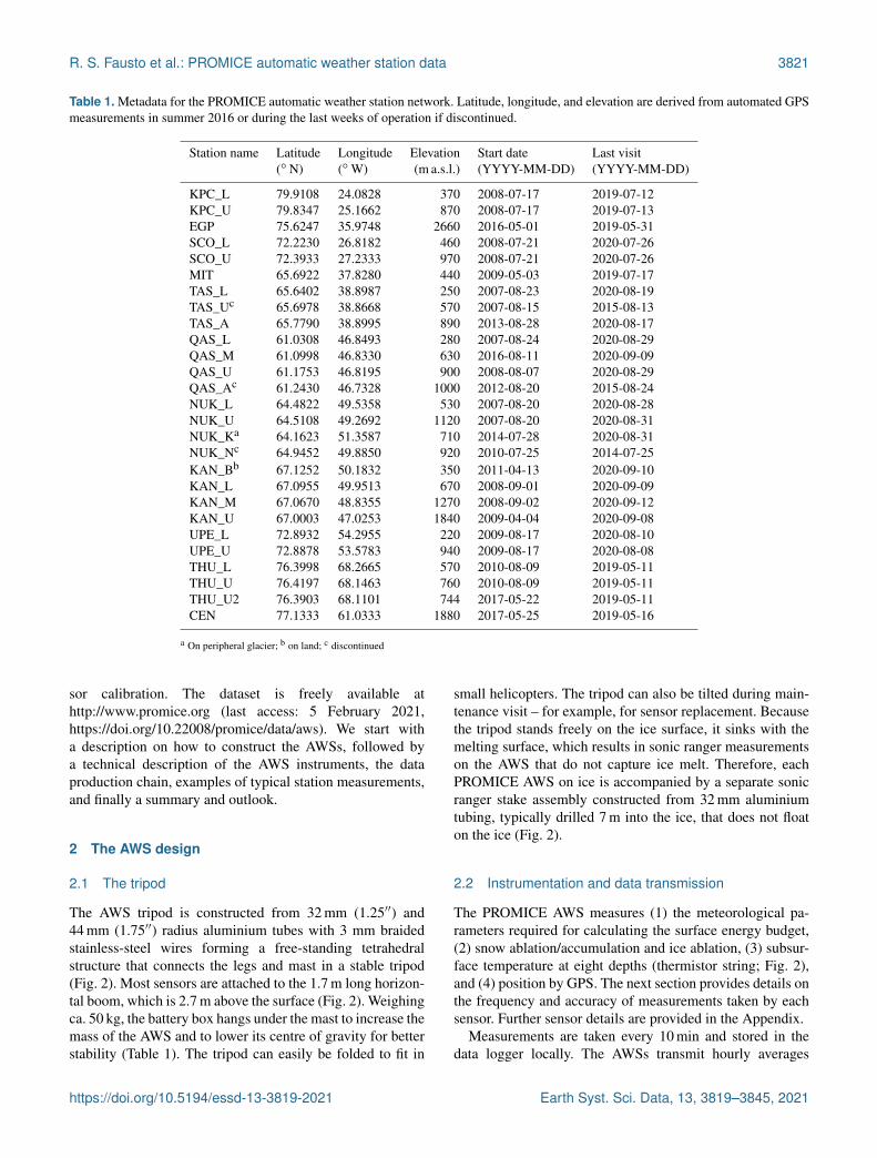
Table 1. Metadata for the PROMICE automatic weather station network. Latitude, longitude, and elevation are derived from automated GPSmeasurements in summer 2016 or during the last weeks of operation if discontinued.

Station name Latitude Longitude Elevation Start date Last visit(◦ N) (◦W) (m a.s.l.) (YYYY-MM-DD) (YYYY-MM-DD)

KPC_L 79.9108 24.0828 370 2008-07-17 2019-07-12KPC_U 79.8347 25.1662 870 2008-07-17 2019-07-13EGP 75.6247 35.9748 2660 2016-05-01 2019-05-31SCO_L 72.2230 26.8182 460 2008-07-21 2020-07-26SCO_U 72.3933 27.2333 970 2008-07-21 2020-07-26MIT 65.6922 37.8280 440 2009-05-03 2019-07-17TAS_L 65.6402 38.8987 250 2007-08-23 2020-08-19TAS_Uc 65.6978 38.8668 570 2007-08-15 2015-08-13TAS_A 65.7790 38.8995 890 2013-08-28 2020-08-17QAS_L 61.0308 46.8493 280 2007-08-24 2020-08-29QAS_M 61.0998 46.8330 630 2016-08-11 2020-09-09QAS_U 61.1753 46.8195 900 2008-08-07 2020-08-29QAS_Ac 61.2430 46.7328 1000 2012-08-20 2015-08-24NUK_L 64.4822 49.5358 530 2007-08-20 2020-08-28NUK_U 64.5108 49.2692 1120 2007-08-20 2020-08-31NUK_Ka 64.1623 51.3587 710 2014-07-28 2020-08-31NUK_Nc 64.9452 49.8850 920 2010-07-25 2014-07-25KAN_Bb 67.1252 50.1832 350 2011-04-13 2020-09-10KAN_L 67.0955 49.9513 670 2008-09-01 2020-09-09KAN_M 67.0670 48.8355 1270 2008-09-02 2020-09-12KAN_U 67.0003 47.0253 1840 2009-04-04 2020-09-08UPE_L 72.8932 54.2955 220 2009-08-17 2020-08-10UPE_U 72.8878 53.5783 940 2009-08-17 2020-08-08THU_L 76.3998 68.2665 570 2010-08-09 2019-05-11THU_U 76.4197 68.1463 760 2010-08-09 2019-05-11THU_U2 76.3903 68.1101 744 2017-05-22 2019-05-11CEN 77.1333 61.0333 1880 2017-05-25 2019-05-16

a On peripheral glacier; b on land; c discontinued

sor calibration. The dataset is freely available athttp://www.promice.org (last access: 5 February 2021,https://doi.org/10.22008/promice/data/aws). We start witha description on how to construct the AWSs, followed bya technical description of the AWS instruments, the dataproduction chain, examples of typical station measurements,and finally a summary and outlook.

2 The AWS design

2.1 The tripod

The AWS tripod is constructed from 32 mm (1.25′′) and44 mm (1.75′′) radius aluminium tubes with 3 mm braidedstainless-steel wires forming a free-standing tetrahedralstructure that connects the legs and mast in a stable tripod(Fig. 2). Most sensors are attached to the 1.7 m long horizon-tal boom, which is 2.7 m above the surface (Fig. 2). Weighingca. 50 kg, the battery box hangs under the mast to increase themass of the AWS and to lower its centre of gravity for betterstability (Table 1). The tripod can easily be folded to fit in

small helicopters. The tripod can also be tilted during main-tenance visit – for example, for sensor replacement. Becausethe tripod stands freely on the ice surface, it sinks with themelting surface, which results in sonic ranger measurementson the AWS that do not capture ice melt. Therefore, eachPROMICE AWS on ice is accompanied by a separate sonicranger stake assembly constructed from 32 mm aluminiumtubing, typically drilled 7 m into the ice, that does not floaton the ice (Fig. 2).

2.2 Instrumentation and data transmission

The PROMICE AWS measures (1) the meteorological pa-rameters required for calculating the surface energy budget,(2) snow ablation/accumulation and ice ablation, (3) subsur-face temperature at eight depths (thermistor string; Fig. 2),and (4) position by GPS. The next section provides details onthe frequency and accuracy of measurements taken by eachsensor. Further sensor details are provided in the Appendix.

Measurements are taken every 10 min and stored in thedata logger locally. The AWSs transmit hourly averages

https://doi.org/10.5194/essd-13-3819-2021 Earth Syst. Sci. Data, 13, 3819–3845, 2021

http://www.promice.org



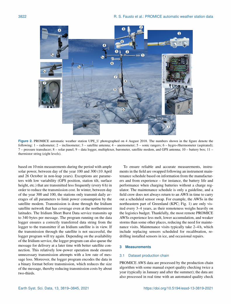
Figure 2. PROMICE automatic weather station UPE_U photographed on 4 August 2018. The numbers shown in the figure denote thefollowing: 1 – radiometer; 2 – inclinometer; 3 – satellite antenna; 4 – anemometer; 5 – sonic rangers; 6 – hygro-/thermometer (aspirated);7 – pressure transducer; 8 – solar panel; 9 – data logger, multiplexer, barometer, satellite modem, and GPS antenna; 10 – battery box; 11 –thermistor string (eight levels).

based on 10 min measurements during the period with amplesolar power, between day of the year 100 and 300 (10 Apriland 26 October in non-leap years). Exceptions are parame-ters with low variability (GPS position, station tilt, surfaceheight, etc.) that are transmitted less frequently (every 6 h) inorder to reduce the transmission cost. In winter, between dayof the year 300 and 100, the stations only transmit daily av-erages of all parameters to limit power consumption by thesatellite modem. Transmission is done through the Iridiumsatellite network that has coverage even at the northernmostlatitudes. The Iridium Short Burst Data service transmits upto 340 bytes per message. The program running on the datalogger ensures a correctly transferred data string from thelogger to the transmitter if an Iridium satellite is in view. Ifthe transmission through the satellite is not successful, thelogger program will try again. Depending on the availabilityof the Iridium service, the logger program can also queue themessage for delivery at a later time with better satellite con-nection. This relatively low-power operation mode ensuresunnecessary transmission attempts with a low rate of mes-sage loss. Moreover, the logger program encodes the data ina binary format before transmission, which reduces the sizeof the message, thereby reducing transmission costs by abouttwo-thirds.

To ensure reliable and accurate measurements, instru-ments in the field are swapped following an instrument main-tenance schedule based on information from the manufactur-ers and from experience – for instance, the battery life andperformance when charging batteries without a charge reg-ulator. The maintenance schedule is only a guideline, and afield crew does not always return to an AWS in time to carryout a scheduled sensor swap. For example, the AWSs in thenortheastern part of Greenland (KPC; Fig. 1) are only vis-ited every 3–4 years, as their remoteness weighs heavily onthe logistics budget. Thankfully, the most remote PROMICEAWSs experience less melt, lower accumulation, and weakerstorms than some other places, reducing the need for mainte-nance visits. Maintenance visits typically take 2–4 h, whichinclude replacing sensors scheduled for recalibration, re-drilling installed sensors in ice, and occasional repairs.

3 Measurements

3.1 Dataset production chain

PROMICE AWS data are processed by the production chainalgorithm with some manual expert quality checking twice ayear (typically in January and after the summer); the data arealso processed in real time with an automated quality check



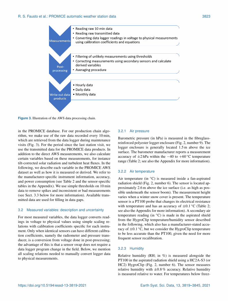
Figure 3. Illustration of the AWS data processing chain.

in the PROMICE database. For our production chain algo-rithm, we make use of the raw data recorded every 10 min,which are retrieved from the data logger during maintenancevisits (Fig. 3). For the period since the last station visit, weuse the transmitted data for the PROMICE data products. Inaddition to the direct AWS measurements, we also calculatecertain variables based on these measurements, for instancetilt-corrected solar radiation and turbulent heat fluxes. In thefollowing, we describe each variable in the PROMICE AWSdataset as well as how it is measured or derived. We refer tothe manufacturer-specific instrument information, accuracy,and power consumption (see Table 2 and the sensor-specifictables in the Appendix). We use simple thresholds on 10 mindata to remove spikes and inconsistent or bad measurements(see Sect. 3.3 below for more information). Available trans-mitted data are used for filling in data gaps.

3.2 Measured variables: description and uncertainty

For most measured variables, the data logger converts read-ings in voltage to physical values using simple scaling re-lations with calibration coefficients specific for each instru-ment. Only when identical sensors can have different calibra-tion coefficients, namely the radiometer and pressure trans-ducer, is a conversion from voltage done in post-processing;the advantage of this is that a sensor swap does not require adata logger program change in the field. Below, we mentionall scaling relations needed to manually convert logger datato physical measurements.

3.2.1 Air pressure

Barometric pressure (in hPa) is measured in the fibreglass-reinforced polyester logger enclosure (Fig. 2, number 9). Thelogger enclosure is generally located 1.5 m above the icesurface. The barometer manufacturer reports a measurementaccuracy of ±2 hPa within the −40 to +60 ◦C temperaturerange (Table 2; see also the Appendix for more information).

3.2.2 Air temperature

Air temperature (in ◦C) is measured inside a fan-aspiratedradiation shield (Fig. 2, number 6). The sensor is located ap-proximately 2.6 m above the ice surface (i.e. as high as pos-sible underneath the sensor boom). The measurement heightvaries when a winter snow cover is present. The temperaturesensor is a PT100 probe that changes its electrical resistancewith temperature and has an accuracy of ±0.1 ◦C (Table 2;see also the Appendix for more information). A secondary airtemperature reading (in ◦C) is made in the aspirated shieldfrom the HygroClip temperature/humidity sensor describedin the following, which also has a manufacturer-stated accu-racy of ±0.1 ◦C, but we consider the HygroClip temperatureto be less accurate than the PT100, given the need for morefrequent sensor recalibration.

3.2.3 Humidity

Relative humidity (RH; in %) is measured alongside thePT100 in the aspirated radiation shield using a HC2A-S3 (orHC2) HygroClip (Fig. 2, number 6). The sensor measuresrelative humidity with ±0.8 % accuracy. Relative humidityis measured relative to water. For temperatures below freez-



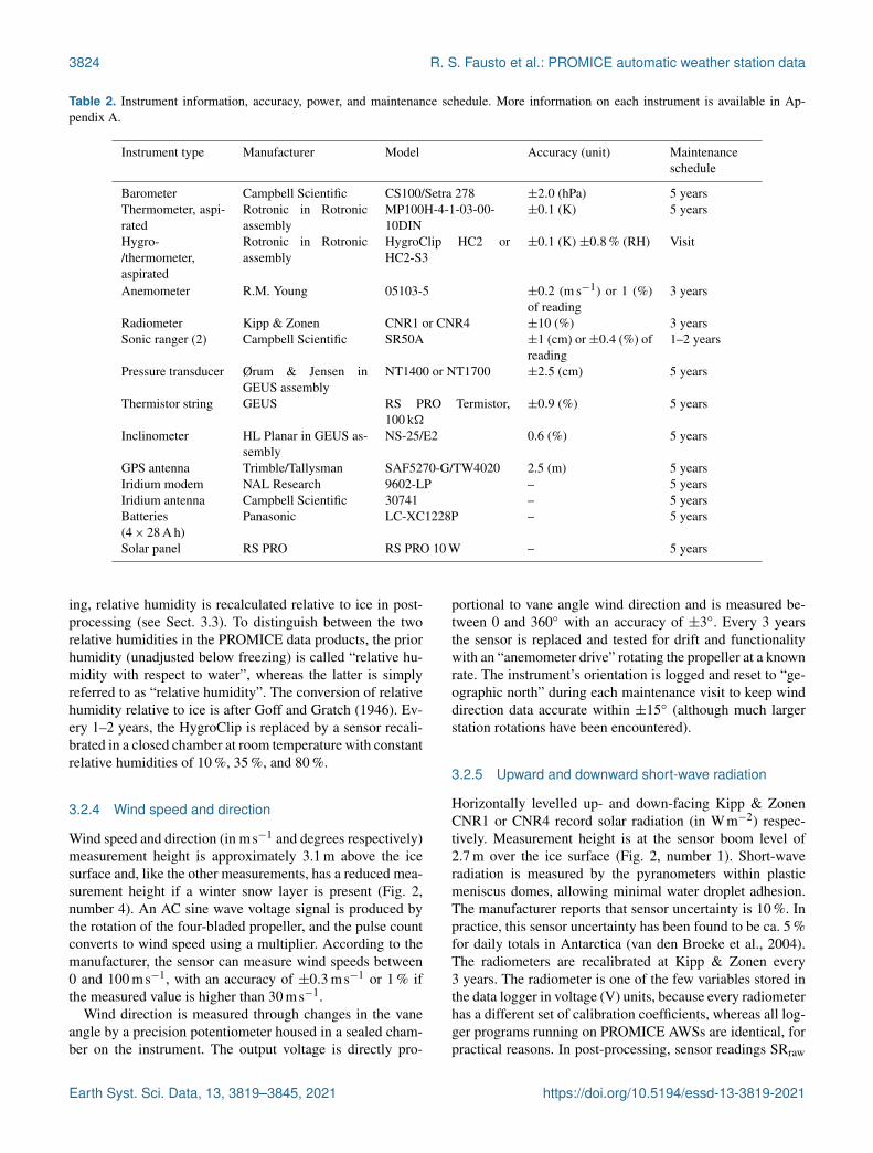
Table 2. Instrument information, accuracy, power, and maintenance schedule. More information on each instrument is available in Ap-pendix A.

Instrument type Manufacturer Model Accuracy (unit) Maintenanceschedule

Barometer Campbell Scientific CS100/Setra 278 ±2.0 (hPa) 5 yearsThermometer, aspi-rated

Rotronic in Rotronicassembly

MP100H-4-1-03-00-10DIN

±0.1 (K) 5 years

Hygro-/thermometer,aspirated

Rotronic in Rotronicassembly

HygroClip HC2 orHC2-S3

±0.1 (K) ±0.8 % (RH) Visit

Anemometer R.M. Young 05103-5 ±0.2 (m s−1) or 1 (%)of reading

3 years

Radiometer Kipp & Zonen CNR1 or CNR4 ±10 (%) 3 yearsSonic ranger (2) Campbell Scientific SR50A ±1 (cm) or±0.4 (%) of

reading1–2 years

Pressure transducer Ørum & Jensen inGEUS assembly

NT1400 or NT1700 ±2.5 (cm) 5 years

Thermistor string GEUS RS PRO Termistor,100 k�

±0.9 (%) 5 years

Inclinometer HL Planar in GEUS as-sembly

NS-25/E2 0.6 (%) 5 years

GPS antenna Trimble/Tallysman SAF5270-G/TW4020 2.5 (m) 5 yearsIridium modem NAL Research 9602-LP – 5 yearsIridium antenna Campbell Scientific 30741 – 5 yearsBatteries(4× 28 A h)

Panasonic LC-XC1228P – 5 years

Solar panel RS PRO RS PRO 10 W – 5 years

ing, relative humidity is recalculated relative to ice in post-processing (see Sect. 3.3). To distinguish between the tworelative humidities in the PROMICE data products, the priorhumidity (unadjusted below freezing) is called “relative hu-midity with respect to water”, whereas the latter is simplyreferred to as “relative humidity”. The conversion of relativehumidity relative to ice is after Goff and Gratch (1946). Ev-ery 1–2 years, the HygroClip is replaced by a sensor recali-brated in a closed chamber at room temperature with constantrelative humidities of 10 %, 35 %, and 80 %.

3.2.4 Wind speed and direction

Wind speed and direction (in ms−1 and degrees respectively)measurement height is approximately 3.1 m above the icesurface and, like the other measurements, has a reduced mea-surement height if a winter snow layer is present (Fig. 2,number 4). An AC sine wave voltage signal is produced bythe rotation of the four-bladed propeller, and the pulse countconverts to wind speed using a multiplier. According to themanufacturer, the sensor can measure wind speeds between0 and 100 ms−1, with an accuracy of ±0.3 ms−1 or 1 % ifthe measured value is higher than 30 ms−1.

Wind direction is measured through changes in the vaneangle by a precision potentiometer housed in a sealed cham-ber on the instrument. The output voltage is directly pro-

portional to vane angle wind direction and is measured be-tween 0 and 360◦ with an accuracy of ±3◦. Every 3 yearsthe sensor is replaced and tested for drift and functionalitywith an “anemometer drive” rotating the propeller at a knownrate. The instrument’s orientation is logged and reset to “ge-ographic north” during each maintenance visit to keep winddirection data accurate within ±15◦ (although much largerstation rotations have been encountered).

3.2.5 Upward and downward short-wave radiation

Horizontally levelled up- and down-facing Kipp & ZonenCNR1 or CNR4 record solar radiation (in Wm−2) respec-tively. Measurement height is at the sensor boom level of2.7 m over the ice surface (Fig. 2, number 1). Short-waveradiation is measured by the pyranometers within plasticmeniscus domes, allowing minimal water droplet adhesion.The manufacturer reports that sensor uncertainty is 10 %. Inpractice, this sensor uncertainty has been found to be ca. 5 %for daily totals in Antarctica (van den Broeke et al., 2004).The radiometers are recalibrated at Kipp & Zonen every3 years. The radiometer is one of the few variables stored inthe data logger in voltage (V) units, because every radiometerhas a different set of calibration coefficients, whereas all log-ger programs running on PROMICE AWSs are identical, forpractical reasons. In post-processing, sensor readings SRraw



are converted into a physical measurement SRm as follows:

SRm =SRraw

CSR, (1)

where CSR (in V(W m−2)−1) is a sensor calibration coeffi-cient, and SRm is either the converted downward or upwardshort-wave irradiance. Short-wave radiation measurementsare corrected for sensor tilt following van As et al. (2011a)in post-processing, which means that the PROMICE AWSdataset contains both uncorrected and corrected values.

3.2.6 Upward and downward long-wave radiation

Long-wave radiation (in W m−2) is also measured by theCNR1/CNR4 radiometer mounted at approximately 2.7 mover the ice surface (Fig. 2, number 1). The radiometer con-tains a pair of up- and down-facing pyrgeometers, with aspectral range of 4.5 to 42 µm. In the same manner as forshort-wave radiation, long-wave radiation is stored in voltageunits (LRraw) in the data logger and transformed to physicalunits (LRm) in post-processing as follows:

LRm =LRraw

CLR+ 5.67× 108

· (Trad+ T0)4, (2)

where CLR (in V (W m−2)−1) is the sensor calibration coeffi-cient, Trad is the sensor temperature measured in the radiome-ter casing (in ◦C), and T0 = 273.15 ◦C.

3.2.7 Surface height

The height of the sensor boom (in metres) is measured by asonic ranger attached to the boom itself approximately 0.1 mbelow the boom (Fig. 2, number 5a), while the height of thestake assembly is measured about 0.1 m below an aluminiumboom connecting stakes drilled into ice (Fig. 2, number 5b).The sensor outputs a distance (Hraw) that requires an air tem-perature correction in post-processing. The temperature ad-justment is performed as follows:

Hm =Hraw ·

√Tair+ T0

T0. (3)

After temperature correction, the measurement uncertaintyof the SR50A sonic ranger reported by the manufacturer(Campbell Scientific) is ±1 cm or ±0.4 % of the mea-sured distance. The uncertainty of sonic ranger readings inPROMICE was investigated utilizing data from a wintertimeaccumulation-free period of more than 2 months at the lo-cation SCO_U. The associated standard deviations for thetwo sensors were found to be 1.7 and 0.6 cm after spike re-moval, amounting to 0.7 % and 0.6 % of the measured dis-tance respectively (Fausto et al., 2012). In addition to the sen-sor uncertainties, occasional problems with the stake assem-bly occurred, primarily in terms of stability during storms

when melted out several metres. Also, an unknown amountof melt-in of the stake assembly can occur, but we speculatethat this only happens (1) when surface melt since installa-tion has been considerable, increasing the height and, thus,the pressure applied by the stake assembly, and (2) when thestake bottoms are not plugged with caps, as was only the caseuntil 2010.

The PROMICE AWSs are also equipped with a pres-sure transducer assembly (PTA) that measures surface heightchange due to ice ablation (Fig. 2, number 7). The assem-bly was first constructed and implemented in Greenland in2001 by Bøggild et al. (2004) but was further developedwithin PROMICE (Fausto et al., 2012). The PTA consists ofa 50 / 50 antifreeze / water mixture-filled hose with a pressuretransducer attached at the bottom. Drilling the hose typicallymore than 10 m into the ice, the pressure signal registered bythe transducer will be that of the vertical liquid column overthe sensor, where the upper level is a bladder fixed on thetripod in a shielded box. This allows inflow/outflow of an-tifreeze due to compression while keeping a steady level atroughly 1.5 m above the ice surface depending on the AWS.Figure 2 illustrates the free-standing AWS tripod that floatson the ice surface and moves down with the ablating sur-face, whereas the hose itself melts out of the ice, which, inturn, will reduce the hydrostatic pressure from the verticalliquid column over the pressure transducer at the bottom ofthe hose. The measured reduction in pressure at the bottomof the hose translates directly into ice ablation. As for theradiometer, every pressure transducer has a different calibra-tion coefficient, which is why measurements are stored inthe data logger in voltage units and transformed to a physicalmeasurement in post-processing. Measurement height (Hm),or in fact depth relative to the PTA bladder, is calculated asfollows:

Hm = CPTA ·ρw

ρaf·Hraw, (4)

where CPTA is the calibration coefficient. The constantsρw and ρaf are the densities of water and the 50 / 50 an-tifreeze / water solution respectively.

3.2.8 Subsurface temperature

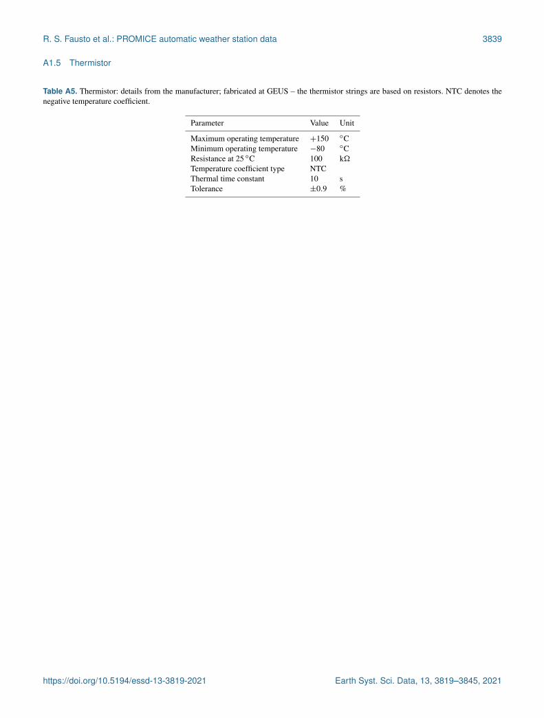
Subsurface temperatures (in ◦C) are measured by a 10 m ther-mistor (temperature-dependent resistor) string (Fig. 2, num-ber 11). The string measures at 1, 2, 3, 4, 5, 6, 7, and 10 mdepth, although depths vary due to the surface ablation andaccumulation. The string is constructed at GEUS (see the Ap-pendix for more information).

3.2.9 Station tilt

The inclinometer is installed on the sensor boom (Fig. 2,number 2) and is aligned with the radiometer to allow fortilt correction of short-wave radiation measurements. The in-clinometer measures the tilt (in degrees) across (left–right)



and along (up–down) the sensor boom, which translates intotilt-to-east and tilt-to-north when the sensor boom is perfectlyoriented north–south. The tilt sensor readings in voltage units(Tiltraw) are converted into tilt in degrees as follows:

Tiltm = 21.1 · |Tiltraw| − 10.4 · |Tiltraw|2

+ 3.6 · |Tiltraw|3− 0.49 · |Tiltraw|

4, (5)

where all constants were determined at GEUS (Table 2).Ice ablation causes the AWS tripod to melt downward; thischanging (slippery) surface often results in AWS tilt changesof more than several degrees.

3.2.10 AWS position

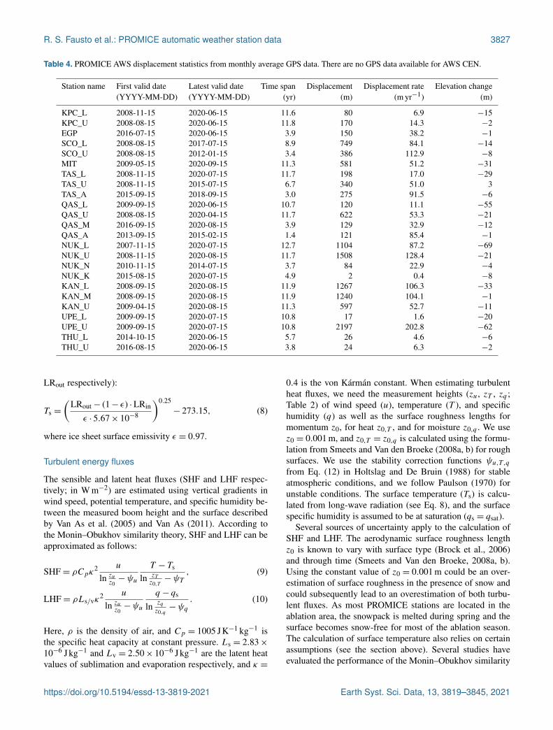
We use a single-frequency GPS receiver to measure the posi-tion (in ◦ N/◦W) and the elevation (metres above sea level) ofeach station to quantify ice flow velocity (Fig. 2, number 9).The GPS antenna, as well as the receiver contained in theIridium 9602-LP modem, is placed inside the data logger en-closure. The receiver type is described as follows: NEO-6Q,1575.42 MHz (L1), 16-channel, and C/A code. The accuracyis reported to be within 2.5 m. In the PROMICE AWS set-up, the GPS receiver is powered up for 5 min preceding eachIridium transmission (hourly in summer and daily in winter),during which it attempts to acquire location data every 20 s.The return (out of a maximum of 15) that reports the lowesthorizontal dilution of precision is written to memory. To date,NUK_U, NUK_L, MIT, and QAS_L have been repositionedduring maintenance visits over distances larger than severaltens of metres. The main reason for this is to reduce the influ-ence of location change on the AWS variables measured, butstations have also been relocated to move them away froma region with opening crevasses. Table 4 shows the horizon-tal and vertical displacement due to glacier flow and AWSrelocation during maintenance visits.

3.3 Post-processing

In this section, we describe and quantify the filtering process,how we correct measurements, and how we calculate derivedvariables in the dataset. The hourly, daily, and monthly aver-aging procedures are also described.

3.3.1 Filtering

Table 5 provides filtering information used in the process-ing chain. We remove unrealistic spikes from the data by us-ing upper and lower thresholds for each measurement. Mea-surements outside these (generous) threshold limits, whichcould occur for a number of known and unknown reasons,are considered erroneous and set to −999. Known reasonswill be discussed in Sect. 4.3 (living data section). Derivedvariables are also set to −999 when one or more of the listed“core” AWS measurements that serve as input fall outside thethreshold limits.

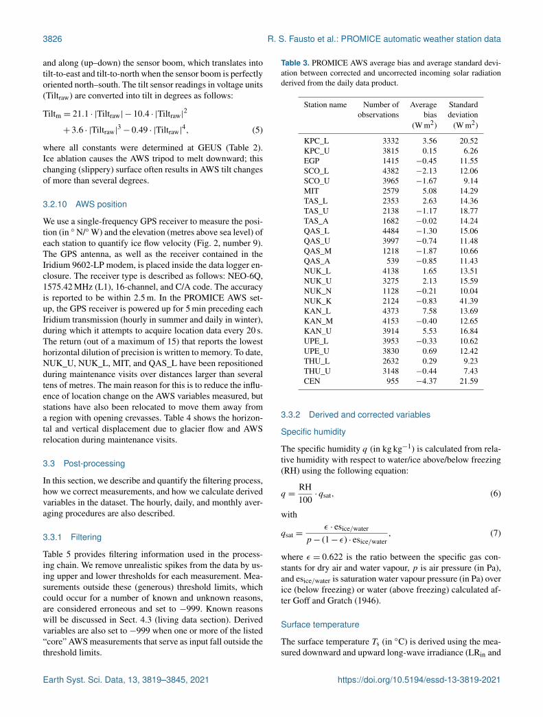
Table 3. PROMICE AWS average bias and average standard devi-ation between corrected and uncorrected incoming solar radiationderived from the daily data product.

Station name Number of Average Standardobservations bias deviation

(W m2) (W m2)

KPC_L 3332 3.56 20.52KPC_U 3815 0.15 6.26EGP 1415 −0.45 11.55SCO_L 4382 −2.13 12.06SCO_U 3965 −1.67 9.14MIT 2579 5.08 14.29TAS_L 2353 2.63 14.36TAS_U 2138 −1.17 18.77TAS_A 1682 −0.02 14.24QAS_L 4484 −1.30 15.06QAS_U 3997 −0.74 11.48QAS_M 1218 −1.87 10.66QAS_A 539 −0.85 11.43NUK_L 4138 1.65 13.51NUK_U 3275 2.13 15.59NUK_N 1128 −0.21 10.04NUK_K 2124 −0.83 41.39KAN_L 4373 7.58 13.69KAN_M 4153 −0.40 12.65KAN_U 3914 5.53 16.84UPE_L 3953 −0.33 10.62UPE_U 3830 0.69 12.42THU_L 2632 0.29 9.23THU_U 3148 −0.44 7.43CEN 955 −4.37 21.59

3.3.2 Derived and corrected variables

Specific humidity

The specific humidity q (in kg kg−1) is calculated from rela-tive humidity with respect to water/ice above/below freezing(RH) using the following equation:

q =RH100· qsat, (6)

with

qsat =ε · esice/water

p− (1− ε) · esice/water, (7)

where ε = 0.622 is the ratio between the specific gas con-stants for dry air and water vapour, p is air pressure (in Pa),and esice/water is saturation water vapour pressure (in Pa) overice (below freezing) or water (above freezing) calculated af-ter Goff and Gratch (1946).

Surface temperature

The surface temperature Ts (in ◦C) is derived using the mea-sured downward and upward long-wave irradiance (LRin and



Table 4. PROMICE AWS displacement statistics from monthly average GPS data. There are no GPS data available for AWS CEN.

Station name First valid date Latest valid date Time span Displacement Displacement rate Elevation change(YYYY-MM-DD) (YYYY-MM-DD) (yr) (m) (m yr−1) (m)

KPC_L 2008-11-15 2020-06-15 11.6 80 6.9 −15KPC_U 2008-08-15 2020-06-15 11.8 170 14.3 −2EGP 2016-07-15 2020-06-15 3.9 150 38.2 −1SCO_L 2008-08-15 2017-07-15 8.9 749 84.1 −14SCO_U 2008-08-15 2012-01-15 3.4 386 112.9 −8MIT 2009-05-15 2020-09-15 11.3 581 51.2 −31TAS_L 2008-11-15 2020-07-15 11.7 198 17.0 −29TAS_U 2008-11-15 2015-07-15 6.7 340 51.0 3TAS_A 2015-09-15 2018-09-15 3.0 275 91.5 −6QAS_L 2009-09-15 2020-06-15 10.7 120 11.1 −55QAS_U 2008-08-15 2020-04-15 11.7 622 53.3 −21QAS_M 2016-09-15 2020-08-15 3.9 129 32.9 −12QAS_A 2013-09-15 2015-02-15 1.4 121 85.4 −1NUK_L 2007-11-15 2020-07-15 12.7 1104 87.2 −69NUK_U 2008-11-15 2020-08-15 11.7 1508 128.4 −21NUK_N 2010-11-15 2014-07-15 3.7 84 22.9 −4NUK_K 2015-08-15 2020-07-15 4.9 2 0.4 −8KAN_L 2008-09-15 2020-08-15 11.9 1267 106.3 −33KAN_M 2008-09-15 2020-08-15 11.9 1240 104.1 −1KAN_U 2009-04-15 2020-08-15 11.3 597 52.7 −11UPE_L 2009-09-15 2020-07-15 10.8 17 1.6 −20UPE_U 2009-09-15 2020-07-15 10.8 2197 202.8 −62THU_L 2014-10-15 2020-06-15 5.7 26 4.6 −6THU_U 2016-08-15 2020-06-15 3.8 24 6.3 −2

LRout respectively):

Ts =

(LRout− (1− ε) ·LRin

ε · 5.67× 10−8

)0.25

− 273.15, (8)

where ice sheet surface emissivity ε = 0.97.

Turbulent energy fluxes

The sensible and latent heat fluxes (SHF and LHF respec-tively; in W m−2) are estimated using vertical gradients inwind speed, potential temperature, and specific humidity be-tween the measured boom height and the surface describedby Van As et al. (2005) and Van As (2011). According tothe Monin–Obukhov similarity theory, SHF and LHF can beapproximated as follows:

SHF= ρCpκ2 u

ln zuz0−ψu

T − Ts

ln zTz0,T−ψT

, (9)

LHF= ρLs/vκ2 u

ln zuz0−ψu

q − qs

ln zqz0,q−ψq

. (10)

Here, ρ is the density of air, and Cp = 1005 JK−1 kg−1 isthe specific heat capacity at constant pressure. Ls = 2.83×10−6 Jkg−1 and Lv = 2.50× 10−6 Jkg−1 are the latent heatvalues of sublimation and evaporation respectively, and κ =

0.4 is the von Kármán constant. When estimating turbulentheat fluxes, we need the measurement heights (zu, zT , zq ;Table 2) of wind speed (u), temperature (T ), and specifichumidity (q) as well as the surface roughness lengths formomentum z0, for heat z0,T , and for moisture z0,q . We usez0 = 0.001 m, and z0,T = z0,q is calculated using the formu-lation from Smeets and Van den Broeke (2008a, b) for roughsurfaces. We use the stability correction functions ψu,T ,qfrom Eq. (12) in Holtslag and De Bruin (1988) for stableatmospheric conditions, and we follow Paulson (1970) forunstable conditions. The surface temperature (Ts) is calcu-lated from long-wave radiation (see Eq. 8), and the surfacespecific humidity is assumed to be at saturation (qs = qsat).

Several sources of uncertainty apply to the calculation ofSHF and LHF. The aerodynamic surface roughness lengthz0 is known to vary with surface type (Brock et al., 2006)and through time (Smeets and Van den Broeke, 2008a, b).Using the constant value of z0 = 0.001 m could be an over-estimation of surface roughness in the presence of snow andcould subsequently lead to an overestimation of both turbu-lent fluxes. As most PROMICE stations are located in theablation area, the snowpack is melted during spring and thesurface becomes snow-free for most of the ablation season.The calculation of surface temperature also relies on certainassumptions (see the section above). Several studies haveevaluated the performance of the Monin–Obukhov similarity



theory in Greenland. Using one- and two-level methods vs.eddy covariance and evaporation lysimeters, Box and Stef-fen (2001) found an underestimation of downward LHF dur-ing extreme stability cases. Miller et al. (2017) used a sim-ilar method for calculating SHF and reported a root-mean-square difference (RMSD) of 8.7 Wm−2, with an averagebias of −7.0 Wm−2, when compared with their two-leveleddy-covariance estimation of SHF. Miller et al. (2017) em-phasized that SHF records from one-level approaches oftencover longer time periods. Fausto et al. (2016a, b) investi-gated the use of an unrealistically high z0 to get agreementbetween surface energy balance (SEB) closure and observedablation rates during extreme sensible and latent heat-drivenmelt events.

Tilt correction of downward short-wave radiation andcloud cover

Tilt correction of solar radiation is performed followingVan As (2011). Downward short-wave radiation (SRin) con-sists of a diffuse and direct beam part. It is only the directbeam part of SRin that requires tilt correction. For a horizon-tal radiation sensor, the direct beam, which equals SRin, isreduced by its diffuse fraction (fdif). For the tilted radiationsensor, SRin is calculated from the measured value, SRin,m,and a correction factor, C, as follows:

SRin,cor = SRin,mC

1− fdif+Cfdif, (11)

with

C = cos(SZA) ·(

sin(d) sin(lat)cos(φsensor)

− sin(d)cos(lat) sin(θsensor)cos(φsensor)+ cos(d)cos(lat)cos(θsensor)cos(w)+ cos(d) sin(lat) sin(θsensor)cos(φsensor)cos(w)

+ cos(d) sin((θsensor) sin(φsensor) sin(w))−1

, (12)

where SZA is the solar zenith angle, d is the sun declination(the angle of the sun above the plane formed by the Earth’sEquator), w is the hour angle (the angle between the sun’scurrent position in the sky and its position at solar noon),lat is the site’s respective latitude in radians, and θsensor andφsensor are the radiometer’s tilt angle and direction respec-tively. The calculation procedures for d , w, and SZA are de-tailed in Vignola (2019). Table 3 illustrates the average biasor correction made for the incoming solar radiation basedon Eq. (11). The standard deviation indicates that the aver-age correction is minor (below 15 Wm−2) for most AWSs,whereas a few AWSs have corrections values spread out overa wider range.

We estimate fdif spanning from 0.2 for clear skies to 1for overcast conditions, while assuming a linear dependency

on the cloud cover fraction (Harrison et al., 2008). We ap-proximate the cloud cover fraction from the dependence ofthe near-surface air temperature (Tair) on LRin (Van As et al.,2005). For this purpose, we calculate a theoretical downwardlong-wave radiation flux corresponding to clear-sky condi-tions using the equation from Swinbank (1963):

LRclear = 5.31× 10−14· (Tair+ T0)6. (13)

We calculate a theoretical downward long-wave radiationflux corresponding to overcast conditions assuming theblack-body radiation as follows:

LRovercast = 5.67× 10−8· (Tair+ T0)4. (14)

The cloud cover (limited to the [0 : 1] range) is then calcu-lated as

cloudcov=LRin−LRclear

LRovercast−LRclear=fdif− 0.2

0.8. (15)

Albedo

Surface broadband solar reflectivity in the 0.3 to 2.5 µmwavelength range, also known as albedo (unitless), is calcu-lated from 10 min tilt-corrected downward and upward solarirradiance data. Hourly averaged albedo values are calculatedfor cases when the sun hits the radiometer top at angles ex-ceeding 20◦ (i.e. when measurements are most reliable forthis sensor type). Daily albedo averages are computed fromavailable hourly data. AWS obstruction of sunlight, casting ashadow within the radiometer’s field of view, may lower thealbedo on average by 0.03 (Kokhanovsky et al., 2020), butthis depends on the surface type and height. Also of relevanceto measured albedo is the contrast of the surface relative tothe AWS battery box, legs, mast, and enclosure, as well aswhether a melt pond forms beneath the AWS. Ryan et al.(2017) examined spatial variograms in unoccupied-aerial-vehicle-derived albedo vs. satellite and PROMICE albedoand found increasing differences for some PROMICE sitestoward the late melt season when the AWS point measure-ments lack representativity of the increasingly inhomoge-neous surface cover. A study by van den Broeke et al. (2004)found a 5 % uncertainty on pyranometer measurements, al-though the manufacturer, Kipp & Zonen, estimates a moreconservative value of 10 % uncertainty. We conservativelyassume 10 % uncertainty in the calculated albedo.

Ice surface height

The pressure transducer assembly (PTA; Fig. 2, sensor 7) set-up is influenced by variations in air pressure. The air pressurecontributions to the measured PTA signal HM are eliminatedusing the following equation:

HL =HM+PC−PA

gρl, (16)



Table 5. Threshold values used in the filtering process for each measured variable.

Variable Units Low threshold High threshold

Pressure hPa 650 1100All temperatures ◦C −80 30Relative humidity % 0 100Wind speed m s−1 0 100Wind direction ◦ 0 360Downward short-wave radiation W m−2

−10 1500Upward short-wave radiation W m−2

−10 1000Downward long-wave radiation W m−2 50 500Upward long-wave radiation W m−2 50 500Sensor boom height m 0.3 3.0Stake assembly height m 0.3 8.0Pressure transducer assembly m 0 30Boom tilt in both directions ◦

−30 30Latitude ◦ N 60 83Longitude ◦W 20 70Elevation m 0 3000Fan current mA 0 200Battery voltage V 0 30

where PA (in hPa) is air pressure, PC (in hPa) is the knownpressure given by the manufacturer to which the sensor wascalibrated, g = 9.82 m s−2 is the gravitational acceleration,and ρl = 1090 kg m−3 is the antifreeze mixture density at0 ◦C. Changes in HL are equal to ice ablation. Fausto et al.(2012, 2016a) compared PTA time series to hose measure-ments manually performed in the field and recorded dis-tances from sonic rangers to quantify instrument inaccura-cies, which were found to be accurate to within 0.04 m.

3.3.3 Averaging

The time reported in our data products specifies thehour/day/month during which the measurements are taken,as opposed to other products that list the exact timestampof the end of the averaging period. Hourly averages are cal-culated from 10 min values if at least one value is available(10 min data are seldom missing). We then calculate daily av-erages from hourly averages if at least 20 values (∼ 80 %) areavailable for a dataset variables with a clear diurnal variabil-ity. Less transient variables require at least one measurementto calculate an average. Lastly, we calculate the monthly av-erages from daily averages if at least 24 values (∼ 80 %) areavailable.

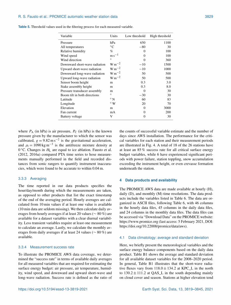
3.3.4 Measurement success rate

To illustrate the PROMICE AWS data coverage, we deter-mined the “success rate” in terms of available daily averagesfor all measured variables that are required for estimating thesurface energy budget: air pressure, air temperature, humid-ity, wind speed, and downward and upward short-wave andlong-wave radiation. Success rate is defined as the ratio of

the counts of successful variable estimate and the number ofdays since AWS installation. The performance for the criti-cal variables for each station and their measurement periodsare illustrated in Fig. 4. A total of 18 of the 26 stations haveat least an 85 % success rate for all critical surface energybudget variables, while 6 have experienced significant peri-ods with power failure, station toppling, snow accumulationexceeding the instrument height, or even crevasse formationunderneath the station.

4 Data products and availability

The PROMICE AWS data are made available at hourly (H),daily (D), and monthly (M) time resolutions. The data prod-ucts include the variables listed in Table 6. The data are or-ganized in ASCII files, following Table 6, with 46 columnsin the hourly data files, 45 columns in the daily data files,and 24 columns in the monthly data files. The data files canbe accessed via “Download Data” on the PROMICE website:https://www.promice.org (last access: 5 February 2021, DOI:https://doi.org/10.22008/promice/data/aws).

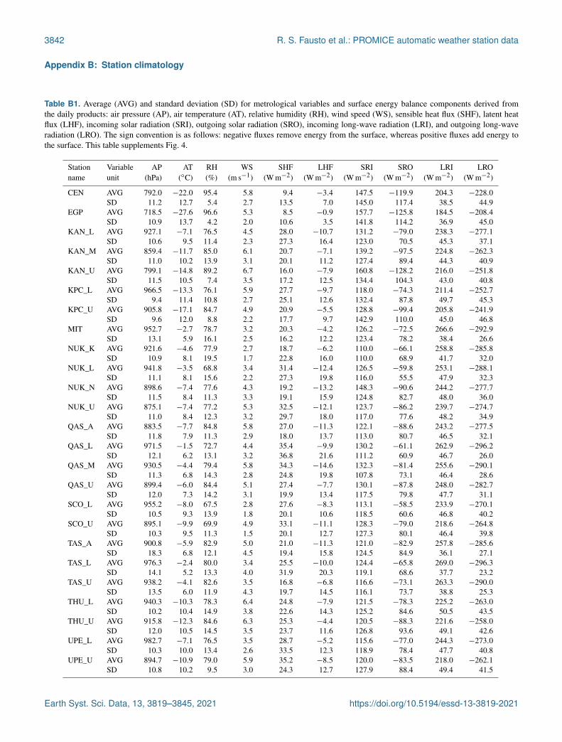
4.1 Data climatology: average and standard deviation

Here, we briefly present the meteorological variables and thesurface energy balance components based on the daily dataproduct. Table B1 shows the average and standard deviationfor all available dataset variables for the 2008–2020 period.In general, Table B1 illustrates that the short-wave radia-tive fluxes vary from 118.0± 134.2 at KPC_L in the northto 130.2± 111.2 at QAS_L in the south depending mainlyon cloud cover and season. Stations at higher elevation tend


https://www.promice.org



Table 6. Short description of all the variables in our data products. An updated version of this short description is kept as a README.txt filein the data product download folder.

Variable in hourly (H), daily (D), Units In data Short descriptionand monthly (M) data products product

Year – H, D, M –MonthOfYear – H, D, M Month of year during which measurements are taken and averaged.DayOfMonth – H, D Day of month during which measurements are taken and averaged.HourOfDay(UTC) UTC H Hour of day during which measurements are taken and averaged.DayOfYear – H, D, M Day of year during which measurements are taken and averaged.DayOfCentury – H, D, M Day of century during which measurements are taken and averaged.AirPressure(hPa) hPa H, D, M Barometric pressure in logger enclosure.AirTemperature(C) ◦C H, D, M Primary air temperature. Measurement height is approximately HeightSensor-

Boom− 0.1 m (or 2.6 m over bare ice surfaces).AirTemperatureHygroClip(C) ◦C H, D, M Secondary air temperature. Measurement height is approximately HeightSensor-

Boom− 0.1 m (or 2.6 m over bare ice surfaces).RelativeHumidity(%) % H, D, M Relative humidity with respect to water/ice above/below freezing. Measurement height

is approximately HeightSensorBoom− 0.1 m (or 2.6 m over bare ice surfaces).SpecificHumidity(g/kg) g kg−1 H, D, M Calculated from RelativeHumidity.WindSpeed(m/s) m s−1 H, D, M Measurement height is approximately HeightSensorBoom+ 0.4 m (or 3.1 m over bare

ice surfaces).WindDirection(d) ◦ H, D, M Measurement height is approximately HeightSensorBoom+ 0.4 m (or 3.1 m over bare

ice surfaces).SensibleHeatFlux(W/m2) W m−2 H, D, M Calculated using gradients of wind speed and temperature between the surface and mea-

surement level. Aerodynamic surface roughness for momentum is set to 0.001 m.LatentHeatFlux(W/m2) W m−2 H, D, M Calculated using gradients of wind speed and humidity between the surface and mea-

surement level. Aerodynamic surface roughness for momentum is set to 0.001 m.ShortwaveRadiationDown(W/m2) W m−2 H, D, M Measurement height is approximately HeightSensorBoom+ 0.1 m (or 2.8 m over bare

ice surfaces).ShortwaveRadiationDown_Cor(W/m2) W m−2 H, D, M Tilt-corrected values calculated from ShortwaveRadiationDown.ShortwaveRadiationUp(W/m2) W m−2 H, D, M Measurement height is approximately HeightSensorBoom+ 0.1 m (or 2.8 m over bare

ice surfaces).ShortwaveRadiationUp_Cor(W/m2) W m−2 H, D, M Tilt-corrected values calculated from ShortwaveRadiationUp.Albedo_theta<70d – H, D, M Surface albedo calculated from ShortwaveRadiationDown_Cor and ShortwaveRadia-

tionUp_Cor using values obtained for solar zenith angles below 70◦.LongwaveRadiationDown(W/m2) W m−2 H, D, M Measurement height is approximately HeightSensorBoom+ 0.1 m (or 2.8 m over bare

ice surfaces).LongwaveRadiationUp(W/m2) W m−2 H, D, M Measurement height is approximately HeightSensorBoom+ 0.1 m (or 2.8 m over bare

ice surfaces).CloudCover % H, D Estimated from LongwaveRadiationDown and AirTemperature.SurfaceTemperature(C) ◦C H, D Calculated from LongwaveRadiationUp and LongwaveRadiationDown. Surface long-

wave emissivity is set to 0.97.HeightSensorBoom(m) m H, D, M Measured at approximately 0.1 m below the sensor boom. The sensitivity of sonic

ranger readings to air temperature is removed.HeightStakes(m) m H, D Measured on a boom connecting aluminium stakes drilled into ice/firn. The sensitivity

of sonic ranger readings to air temperature is removed.DepthPressureTransducer(m) m H, D Typically drilled > 10 m into ice, decreases as ablation occurs.DepthPressureTransducer_Cor(m) m H, D Air pressure contributions eliminated from DepthPressureTransducer.AblationPressureTransducer(mm) mm D Daily ablation estimate from pressure transducer. Only in the daily file.IceTemperature1–8(C) ◦C H, D Subsurface temperature installed at 1, 2, 3, 4, 5, 6, 7, and 10 m depth at ablation-area

sites. Note that the thermistor strings in the ablation area will melt out.TiltToEast(d) ◦ H, D Station tilt towards the east. Station may have rotated.TiltToNorth(d) ◦ H, D Station tilt towards the north. Station may have rotated.TimeGPS(hhmmssUTC) UTC H, D GPS timestamp.LatitudeGPS(degN) ◦ N H, D, M Daily and monthly averages are only calculated using HorDilOfPrecGPS values smaller

than 1.LongitudeGPS(degW) ◦W H, D, M Daily and monthly averages are only calculated using HorDilOfPrecGPS values smaller

than 1.ElevationGPS(m) m H, D, M Daily and monthly averages are only calculated using HorDilOfPrecGPS values smaller

than 1.HorDilOfPrecGPS – H, D GPS horizontal dilution of precision (HDOP) value.LoggerTemperature(C) ◦C H, D Temperature measured by the data logger in the enclosure at 1–1.5 m above the bare ice

surface.FanCurrent(mA) mA H, D Current drawn for ventilation of the temperature and humidity assembly. Normal values

exceed 100 mA.FanOK(%) % M Percentage of time with sufficient ventilation of the temperature and humidity assembly.

Only in the monthly file.BatteryVoltage(V) V H, D Voltage of the four 28 A h batteries. Ventilation of the temperature and humidity assem-

bly, and GPS positioning, stop below 11.5 V.



Figure 4. Combined availability of the eight critical variables required for surface energy balance calculation from PROMICE daily products.See the Appendix for the data availability of each of the variables.

to get more sunlight than the lower-lying stations (van Aset al., 2013; Fausto et al., 2016b). The turbulent fluxes (sen-sible and latent heat) show a positive contribution from thesensible heat flux and a negative contribution from the latentheat flux, both with a considerable variation. The turbulentfluxes are on average lower in magnitude than the radiativefluxes and tend to be higher at lower latitudes and elevation(Fausto et al., 2016b). The temperature is generally higherfor stations located at lower elevations close to the ice sheetmargin, as they are more exposed to the relatively warm at-mospheric conditions of the ocean all year round, except forstations at higher latitudes (above 70◦ N) which experiencesea ice conditions during winter that influence the tempera-ture (van As et al., 2011a, 2014b). Table B1 also illustratesthat the temperature has a clear dependence on latitude andelevation. On average, the wind speed tends to increase withelevation, which is mainly due to the surface radiative cool-ing during winter (van As et al., 2014b).

4.2 Data examples

To create a quick insight into the data product, we show ex-amples of data from AWSs in two contrasting locations: TASin southeast Greenland near Tasiilaq and UPE in northwestGreenland near Upernavik (Fig. 1).

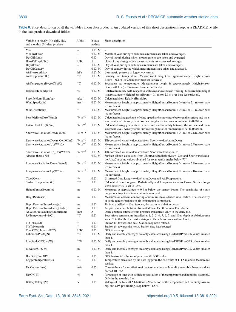
4.2.1 Wind speed

Time series spanning the years 2012 through 2014 of weeklymedian wind speeds and maximum 10 min wind speedwithin that week for TAS_L and UPE_U are displayed inFig. 5. Median wind speeds are lower at TAS_L than atUPE_U, whereas the opposite is true for maximum windspeeds because TAS_L is located in a region well-known forits piteraq storms.



Figure 5. Weekly median wind speeds vs. maximum 10 min wind speed within that week.

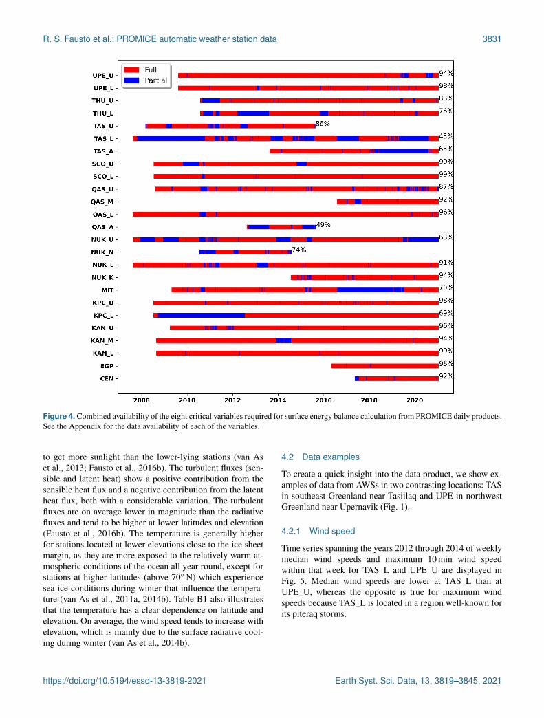
Figure 6. Daily air temperatures from UPE_L and UPE_U.

4.2.2 Air temperature

The daily average air temperature for the two stations nearUpernavik is shown in Fig. 6. The temperature is higher at thelower station, UPE_L, than at the upper station, UPE_U, dueto an elevation difference of more than 700 m. The tendencyof the temperature to have a higher variability during wintermonths than during summer is also evident from these timeseries.

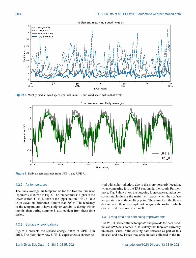
4.2.3 Surface energy balance

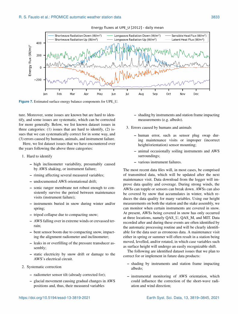
Figure 7 presents the surface energy fluxes at UPE_U in2012. The plots show how UPE_U experiences a shorter pe-

riod with solar radiation, due to the more northerly location,when comparing it to the TAS stations further south. Further-more, Fig. 7 shows how the outgoing long-wave radiation be-comes stable during the main melt season when the surfacetemperature is at the melting point. The sum of all the fluxesdetermines if there is a surplus of energy at the surface, whichcan be used for snow or ice melt.

4.3 Living data and continuing improvements

PROMICE will continue to update and provide the data prod-ucts as AWS data comes in. It is likely that there are currentlyunknown issues in the existing data released as part of thisdataset, and new issues may arise in data collected in the fu-



Figure 7. Estimated surface energy balance components for UPE_U.

ture. Moreover, some issues are known but are hard to iden-tify, and some issues are systematic, which can be correctedfor more generally. Below, we list known dataset issues inthree categories: (1) issues that are hard to identify, (2) is-sues that we can systematically correct for in some way, and(3) errors caused by humans, animals, and instrument failure.

Here, we list dataset issues that we have encountered overthe years following the above three categories:

1. Hard to identify

– high inclinometer variability, presumably causedby AWS shaking, or instrument failure;

– riming affecting several measured variables;

– undocumented AWS orientational drift;

– sonic ranger membrane not robust enough to con-sistently survive the period between maintenancevisits (instrument failure);

– instruments buried in snow during winter and/orspring;

– tripod collapse due to compacting snow;

– AWS falling over in extreme winds or crevassed ter-rain;

– bent sensor boom due to compacting snow, impact-ing the alignment radiometer and inclinometer;

– leaks in or overfilling of the pressure transducer as-sembly;

– static electricity by snow drift or damage to theAWS’s electrical circuit.

2. Systematic correction

– radiometer sensor tilt (already corrected for);

– glacial movement causing gradual changes in AWSpositions and, thus, their measured variables

– shading by instruments and station frame impactingmeasurements (e.g. albedo).

3. Errors caused by humans and animals

– human error, such as sensor plug swap dur-ing maintenance visits or improper (incorrectheight/orientation) sensor mounting;

– animal occasionally soiling instruments and AWSsurroundings;

– various instrument failures.

The most recent data files will, in most cases, be comprisedof transmitted data, which will be updated after the nextmaintenance visit. Data download from the logger will im-prove data quality and coverage. During strong winds, theAWSs can topple or sensors can break down. AWSs can alsobe covered by snow that accumulates in winter, which re-duces the data quality for many variables. Using our heightmeasurements on both the station and the stake assembly, wecan monitor when certain instruments are covered in snow.At present, AWSs being covered in snow has only occurredat three locations, namely QAS_U, QAS_M, and MIT. Datarecorded after and during these events are often identified bythe automatic processing routine and will be clearly identifi-able for the data user as erroneous data. A maintenance visiteither in spring or summer will often result in a station beingmoved, levelled, and/or rotated, in which case variables suchas surface height will undergo an easily recognizable shift.

The following are identified dataset issues that we plan tocorrect for or implement in future data products:

– shading by instruments and station frame impactingalbedo;

– instrumental monitoring of AWS orientation, whichcould influence the correction of the short-wave radi-ation and wind direction;



– instrumental monitoring of rain;

– flagging protocol for identified errors and issues.

While we do our best to clean the data appropriatelyand address known issues (see above), we recognize thatcorrecting issues is more complicated than simply doc-umenting them and that some corrections may not bepossible or may be subjective and a function of differ-ent use cases. Therefore, we introduce a user-contributabledynamic web-based database of known data quality is-sues at https://github.com/GEUS-Glaciology-and-Climate/PROMICE-AWS-data-issues/ (last access: 7 April 2021).The current implementation uses GitHub “issues”, althougha future version may use a different database at the back endthat the DOI would resolve. Each issue is tagged with sta-tion(s), sensor(s), and year(s) where the issue occurs. Userswho are working with a station, sensor, or time frame of dataare encouraged to search the issue database and see if thereare any known relevant data issues. If users discover a dataissue that is not currently documented, they can add it to thedatabase. A PROMICE team member will review and tag anyissues as verified and then suggest a fix. Future versions ofthe product will implement these fixes if possible, and theissues will be closed but remain accessible.

5 Data availability

The PROMICE AWS product is available fromhttps://doi.org/10.22008/promice/data/aws (Fausto et al.,2019).

6 Code availability

The processing code is available athttps://doi.org/10.22008/W19C-B256 (van As et al.,2021).

7 Summary and outlook

The UN Intergovernmental Panel on Climate Change (IPCC)has previously highlighted the value of station-level recordsfor assessing the cryospheric changes associated with globalclimate change (Vaughan et al., 2013). The IPCC has morerecently highlighted the importance of understanding Green-land Ice Sheet mass loss, especially mass loss due to atmo-spheric forcing and surface mass balance mechanisms, as aleading contributor to sea level rise (Meredith et al., 2019).Meteorological and glaciological monitoring sites on the icesheet are necessary to provide well-constrained observationsof surface energy and mass balances. Understanding theselocal energy and mass balances provides the process-levelknowledge of ice sheet and atmosphere interactions requiredby regional and global simulations (e.g. Van As, 2011; Faustoet al., 2016b). The PROMICE network plays a leading role

in providing these in situ observations and process-level in-sights for the Greenland Ice Sheet.

The PROMICE AWS v3 data products are made avail-able as hourly, daily, and monthly data files. All data prod-ucts undergo periodical improvement through updates in theprocessing chain. Data are added as they are received fromfield parties and via satellite transmission. Between 2007and 2021, the PROMICE AWSs have carried out measure-ments with an 85 % success rate for 18 of the 26 stations,defined as the availability fraction of the daily averages forvariables required for calculating the surface energy balance(see Fig. 4). All PROMICE AWS data products are availableat https://doi.org/10.22008/promice/data/aws.

In addition to advancing science, the PROMICE AWSnetwork is now poised to contribute to operational prod-ucts. With recent advances in the quality and trans-parency of the PROMICE data delivery pipeline describedhere, as well as the increasing prevalence of machine-to-machine transfer protocols among data users, the en-tire PROMICE station data archive – including near-real-time observations – is now readily available to ingest inweather forecast and climate reanalysis applications. Withthe original AWS stations quickly approaching their 15thanniversary, the PROMICE data record is crossing thehalfway mark of a 30-year climatological reference period.With the launch of the PROMICE AWS data issues onGitHub (https://github.com/GEUS-Glaciology-and-Climate/PROMICE-AWS-data-issues/, last access: 7 April 2021), wehope to continue to support the growing PROMICE usercommunity into the next decade.





https://doi.org/10.22008/W19C-B256





Appendix A: Sensor tables

A1 Instrument information, accuracy, and powerconsumption

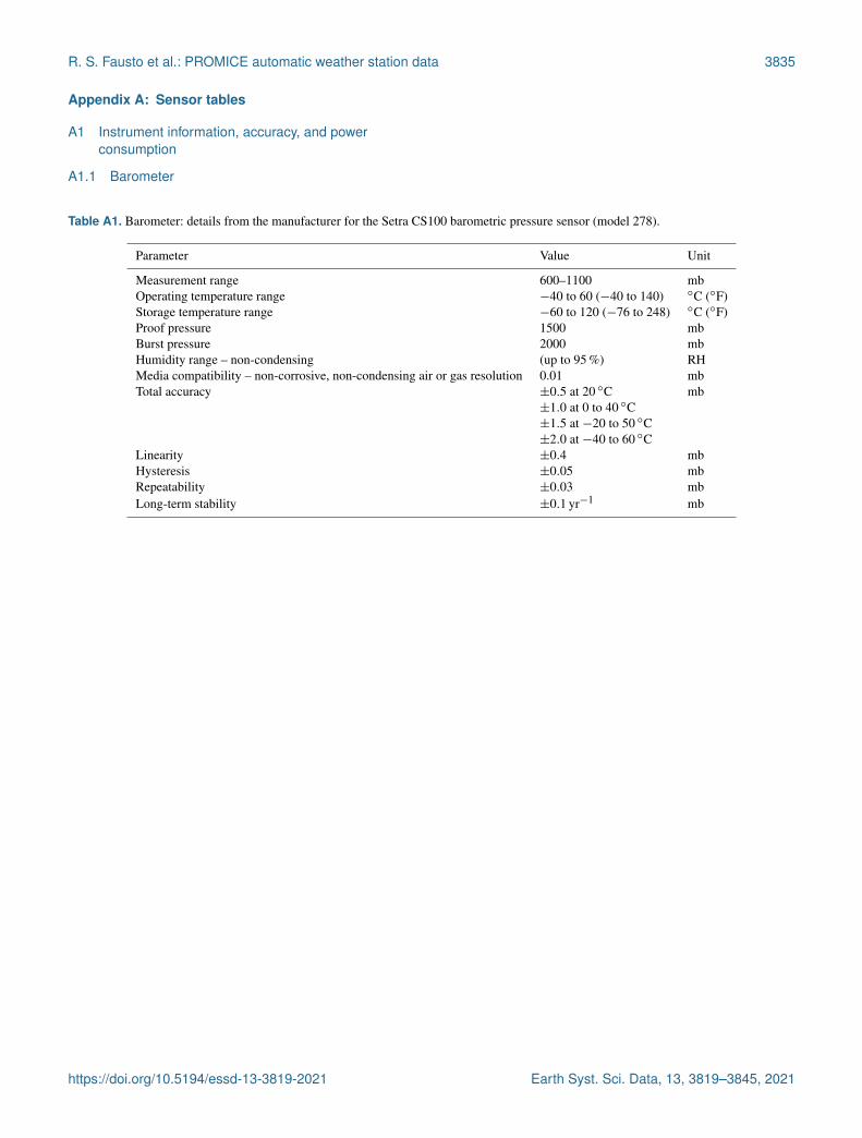
A1.1 Barometer

Table A1. Barometer: details from the manufacturer for the Setra CS100 barometric pressure sensor (model 278).

Parameter Value Unit

Measurement range 600–1100 mbOperating temperature range −40 to 60 (−40 to 140) ◦C (◦F)Storage temperature range −60 to 120 (−76 to 248) ◦C (◦F)Proof pressure 1500 mbBurst pressure 2000 mbHumidity range – non-condensing (up to 95 %) RHMedia compatibility – non-corrosive, non-condensing air or gas resolution 0.01 mbTotal accuracy ±0.5 at 20 ◦C mb

±1.0 at 0 to 40 ◦C±1.5 at −20 to 50 ◦C±2.0 at −40 to 60 ◦C

Linearity ±0.4 mbHysteresis ±0.05 mbRepeatability ±0.03 mbLong-term stability ±0.1 yr−1 mb



A1.2 Thermometer and hygrometer

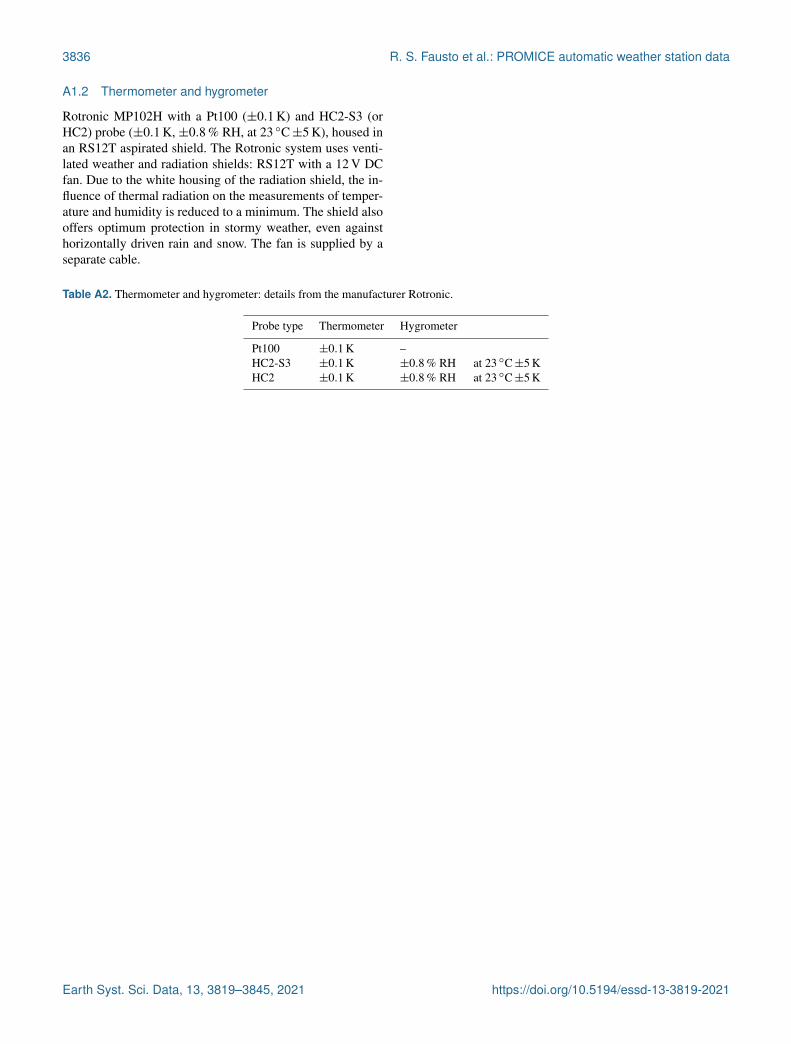
Rotronic MP102H with a Pt100 (±0.1 K) and HC2-S3 (orHC2) probe (±0.1 K, ±0.8 % RH, at 23 ◦C±5 K), housed inan RS12T aspirated shield. The Rotronic system uses venti-lated weather and radiation shields: RS12T with a 12 V DCfan. Due to the white housing of the radiation shield, the in-fluence of thermal radiation on the measurements of temper-ature and humidity is reduced to a minimum. The shield alsooffers optimum protection in stormy weather, even againsthorizontally driven rain and snow. The fan is supplied by aseparate cable.

Table A2. Thermometer and hygrometer: details from the manufacturer Rotronic.

Probe type Thermometer Hygrometer

Pt100 ±0.1 K –HC2-S3 ±0.1 K ±0.8 % RH at 23 ◦C±5 KHC2 ±0.1 K ±0.8 % RH at 23 ◦C±5 K



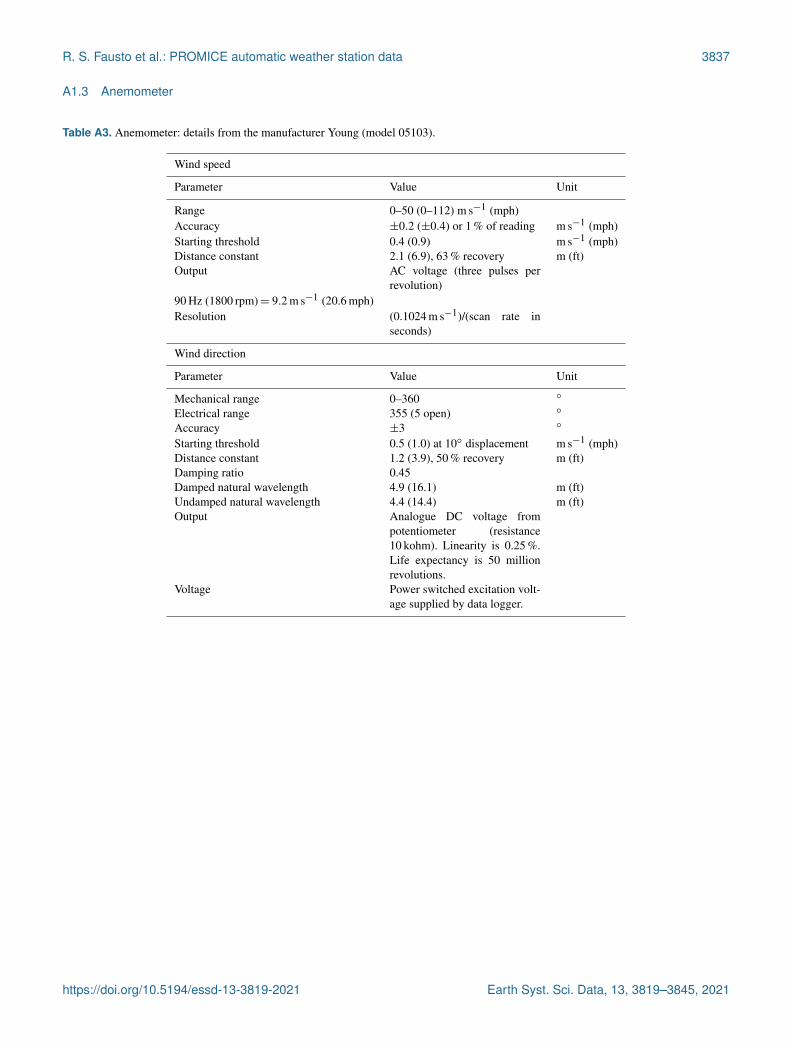
A1.3 Anemometer

Table A3. Anemometer: details from the manufacturer Young (model 05103).

Wind speed


Range 0–50 (0–112) m s−1 (mph)Accuracy ±0.2 (±0.4) or 1 % of reading m s−1 (mph)Starting threshold 0.4 (0.9) m s−1 (mph)Distance constant 2.1 (6.9), 63 % recovery m (ft)Output AC voltage (three pulses per

revolution)90 Hz (1800 rpm)= 9.2 m s−1 (20.6 mph)Resolution (0.1024 m s−1)/(scan rate in

seconds)

Wind direction


Mechanical range 0–360 ◦

Electrical range 355 (5 open) ◦

Accuracy ±3 ◦

Starting threshold 0.5 (1.0) at 10◦ displacement m s−1 (mph)Distance constant 1.2 (3.9), 50 % recovery m (ft)Damping ratio 0.45Damped natural wavelength 4.9 (16.1) m (ft)Undamped natural wavelength 4.4 (14.4) m (ft)Output Analogue DC voltage from

potentiometer (resistance10 kohm). Linearity is 0.25 %.Life expectancy is 50 millionrevolutions.

Voltage Power switched excitation volt-age supplied by data logger.



A1.4 Radiometer

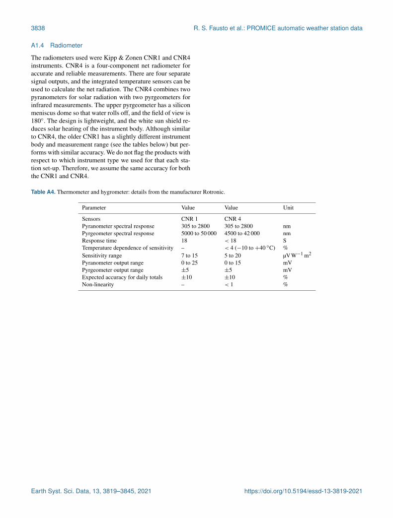
The radiometers used were Kipp & Zonen CNR1 and CNR4instruments. CNR4 is a four-component net radiometer foraccurate and reliable measurements. There are four separatesignal outputs, and the integrated temperature sensors can beused to calculate the net radiation. The CNR4 combines twopyranometers for solar radiation with two pyrgeometers forinfrared measurements. The upper pyrgeometer has a siliconmeniscus dome so that water rolls off, and the field of view is180◦. The design is lightweight, and the white sun shield re-duces solar heating of the instrument body. Although similarto CNR4, the older CNR1 has a slightly different instrumentbody and measurement range (see the tables below) but per-forms with similar accuracy. We do not flag the products withrespect to which instrument type we used for that each sta-tion set-up. Therefore, we assume the same accuracy for boththe CNR1 and CNR4.

Table A4. Thermometer and hygrometer: details from the manufacturer Rotronic.

Parameter Value Value Unit

Sensors CNR 1 CNR 4Pyranometer spectral response 305 to 2800 305 to 2800 nmPyrgeometer spectral response 5000 to 50 000 4500 to 42 000 nmResponse time 18 < 18 STemperature dependence of sensitivity – < 4 (−10 to +40 ◦C) %Sensitivity range 7 to 15 5 to 20 µVW−1 m2

Pyranometer output range 0 to 25 0 to 15 mVPyrgeometer output range ±5 ±5 mVExpected accuracy for daily totals ±10 ±10 %Non-linearity – < 1 %



A1.5 Thermistor

Table A5. Thermistor: details from the manufacturer; fabricated at GEUS – the thermistor strings are based on resistors. NTC denotes thenegative temperature coefficient.


Maximum operating temperature +150 ◦CMinimum operating temperature −80 ◦CResistance at 25 ◦C 100 k�Temperature coefficient type NTCThermal time constant 10 sTolerance ±0.9 %



A1.6 Inclinometer

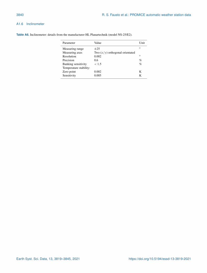
Table A6. Inclinometer: details from the manufacturer HL Planartechnik (model NS-25/E2).


Measuring range ±25 ◦

Measuring axes Two (x/y) orthogonal orientatedResolution 0.002 ◦

Precision 0.6 %Banking sensitivity < 1.5 %Temperature stability:Zero point 0.002 KSensitivity 0.005 K



A1.7 Sonic rangers

The accuracy of the SR50A sonic ranger given by the man-ufacturer (Campbell Scientific) is ±1 cm or ±0.4 % of themeasuring height after temperature correction.

A1.8 Pressure transducer

The PROMICE AWSs are equipped with an Ørum & JensenNT1400/NT1700 pressure transducer assembly (PTA). ThePTA monitors ice surface height change due to ablation. Thepressure transducer sensor has an accuracy of 2.5 cm givenby the manufacturer.

A1.9 GPS

We have equipped a single-frequency GPS. It is built intoan Iridium 9602-LP modem. The manufacturer describes thereceiver type in the following way: NEO-6Q, 1575.42 MHz(L1), 16-channel, C/A code; accuracy of 2.5 m CEP (circularerror probable); update rate of 5 Hz; start-up times of 1 s forhot starts and 28 s for warm starts and cold starts; sensitivityof −160 dBm.



Appendix B: Station climatology

Table B1. Average (AVG) and standard deviation (SD) for metrological variables and surface energy balance components derived fromthe daily products: air pressure (AP), air temperature (AT), relative humidity (RH), wind speed (WS), sensible heat flux (SHF), latent heatflux (LHF), incoming solar radiation (SRI), outgoing solar radiation (SRO), incoming long-wave radiation (LRI), and outgoing long-waveradiation (LRO). The sign convention is as follows: negative fluxes remove energy from the surface, whereas positive fluxes add energy tothe surface. This table supplements Fig. 4.

Station Variable AP AT RH WS SHF LHF SRI SRO LRI LROname unit (hPa) (◦C) (%) (m s−1) (W m−2) (W m−2) (W m−2) (W m−2) (W m−2) (W m−2)

CEN AVG 792.0 −22.0 95.4 5.8 9.4 −3.4 147.5 −119.9 204.3 −228.0SD 11.2 12.7 5.4 2.7 13.5 7.0 145.0 117.4 38.5 44.9

EGP AVG 718.5 −27.6 96.6 5.3 8.5 −0.9 157.7 −125.8 184.5 −208.4SD 10.9 13.7 4.2 2.0 10.6 3.5 141.8 114.2 36.9 45.0

KAN_L AVG 927.1 −7.1 76.5 4.5 28.0 −10.7 131.2 −79.0 238.3 −277.1SD 10.6 9.5 11.4 2.3 27.3 16.4 123.0 70.5 45.3 37.1

KAN_M AVG 859.4 −11.7 85.0 6.1 20.7 −7.1 139.2 −97.5 224.8 −262.3SD 11.0 10.2 13.9 3.1 20.1 11.2 127.4 89.4 44.3 40.9

KAN_U AVG 799.1 −14.8 89.2 6.7 16.0 −7.9 160.8 −128.2 216.0 −251.8SD 11.5 10.5 7.4 3.5 17.2 12.5 134.4 104.3 43.0 40.8

KPC_L AVG 966.5 −13.3 76.1 5.9 27.7 −9.7 118.0 −74.3 211.4 −252.7SD 9.4 11.4 10.8 2.7 25.1 12.6 132.4 87.8 49.7 45.3

KPC_U AVG 905.8 −17.1 84.7 4.9 20.9 −5.5 128.8 −99.4 205.8 −241.9SD 9.6 12.0 8.8 2.2 17.7 9.7 142.9 110.0 45.0 46.8

MIT AVG 952.7 −2.7 78.7 3.2 20.3 −4.2 126.2 −72.5 266.6 −292.9SD 13.1 5.9 16.1 2.5 16.2 12.2 123.4 78.2 38.4 26.6

NUK_K AVG 921.6 −4.6 77.9 2.7 18.7 −6.2 110.0 −66.1 258.8 −285.8SD 10.9 8.1 19.5 1.7 22.8 16.0 110.0 68.9 41.7 32.0

NUK_L AVG 941.8 −3.5 68.8 3.4 31.4 −12.4 126.5 −59.8 253.1 −288.1SD 11.1 8.1 15.6 2.2 27.3 19.8 116.0 55.5 47.9 32.3

NUK_N AVG 898.6 −7.4 77.6 4.3 19.2 −13.2 148.3 −90.6 244.2 −277.7SD 11.5 8.4 11.3 3.3 19.1 15.9 124.8 82.7 48.0 36.0

NUK_U AVG 875.1 −7.4 77.2 5.3 32.5 −12.1 123.7 −86.2 239.7 −274.7SD 11.0 8.4 12.3 3.2 29.7 18.0 117.0 77.6 48.2 34.9

QAS_A AVG 883.5 −7.7 84.8 5.8 27.0 −11.3 122.1 −88.6 243.2 −277.5SD 11.8 7.9 11.3 2.9 18.0 13.7 113.0 80.7 46.5 32.1

QAS_L AVG 971.5 −1.5 72.7 4.4 35.4 −9.9 130.2 −61.1 262.9 −296.2SD 12.1 6.2 13.1 3.2 36.8 21.6 111.2 60.9 46.7 26.0

QAS_M AVG 930.5 −4.4 79.4 5.8 34.3 −14.6 132.3 −81.4 255.6 −290.1SD 11.3 6.8 14.3 2.8 24.8 19.8 107.8 73.1 46.4 28.6

QAS_U AVG 899.4 −6.0 84.4 5.1 27.4 −7.7 130.1 −87.8 248.0 −282.7SD 12.0 7.3 14.2 3.1 19.9 13.4 117.5 79.8 47.7 31.1

SCO_L AVG 955.2 −8.0 67.5 2.8 27.6 −8.3 113.1 −58.5 233.9 −270.1SD 10.5 9.3 13.9 1.8 20.1 10.6 118.5 60.6 46.8 40.2

SCO_U AVG 895.1 −9.9 69.9 4.9 33.1 −11.1 128.3 −79.0 218.6 −264.8SD 10.3 9.5 11.3 1.5 20.1 12.7 127.3 80.1 46.4 39.8

TAS_A AVG 900.8 −5.9 82.9 5.0 21.0 −11.3 121.0 −82.9 257.8 −285.6SD 18.3 6.8 12.1 4.5 19.4 15.8 124.5 84.9 36.1 27.1

TAS_L AVG 976.3 −2.4 80.0 3.4 25.5 −10.0 124.4 −65.8 269.0 −296.3SD 14.1 5.2 13.3 4.0 31.9 20.3 119.1 68.6 37.7 23.2

TAS_U AVG 938.2 −4.1 82.6 3.5 16.8 −6.8 116.6 −73.1 263.3 −290.0SD 13.5 6.0 11.9 4.3 19.7 14.5 116.1 73.7 38.8 25.3

THU_L AVG 940.3 −10.3 78.3 6.4 24.8 −7.9 121.5 −78.3 225.2 −263.0SD 10.2 10.4 14.9 3.8 22.6 14.3 125.2 84.6 50.5 43.5

THU_U AVG 915.8 −12.3 84.6 6.3 25.3 −4.4 120.5 −88.3 221.6 −258.0SD 12.0 10.5 14.5 3.5 23.7 11.6 126.8 93.6 49.1 42.6

UPE_L AVG 982.7 −7.1 76.5 3.5 28.7 −5.2 115.6 −77.0 244.3 −273.0SD 10.3 10.0 13.4 2.6 33.5 12.3 118.9 78.4 47.7 40.8

UPE_U AVG 894.7 −10.9 79.0 5.9 35.2 −8.5 120.0 −83.5 218.0 −262.1SD 10.8 10.2 9.5 3.0 24.3 12.7 127.9 88.4 49.4 41.5



Author contributions. AA, SA, DvA, and RF designed, man-aged, and received funding for the PROMICE monitoring pro-gramme for the 2007–2021 period. RF and DvA produced thePROMICE AWS product. RF and KM set up the data curationframework. MC, AP, CS, RF, and DvA contributed to the sensorand AWS design. SN also contributed to the sensor and AWS de-sign but passed away before submission; we regard their approvalof this work as implicit. RF, BV, JB, WC, and KM contributed tothe data analysis and validation. RF, AS, SL, NK, KK, NK, and JBwere responsible for the data product description, data climatology,and data examples. All authors carried out the data assimilation. RFprepared the paper with contributions from all co-authors.

Competing interests. The authors declare that they have no con-flict of interest.

Disclaimer. Publisher’s note: Copernicus Publications remainsneutral with regard to jurisdictional claims in published maps andinstitutional affiliations.

Special issue statement. This article is part of the special issue“Extreme environment datasets for the three poles”. It is not associ-ated with a conference.

Acknowledgements. AWS data from the Programme for Moni-toring of the Greenland Ice Sheet (PROMICE) and the GreenlandAnalogue Project (GAP) were provided by the Geological Surveyof Denmark and Greenland (GEUS) at https://www.promice.org(last access: 5 February 2021). We would like to thank the editor,David Carlson; one anonymous reviewer; and Jacob C. Yde for theirthoughtful comments and suggestions.

Financial support. This research has been supported by the Min-istry of Climate, Energy, and Utilities through the Danish Coopera-tion for Environment in the Arctic.

Review statement. This paper was edited by David Carlson andreviewed by Jacob Yde and one anonymous referee.

References

Ahlstrøm, A. P., Gravesen, P., Andersen, S. B., van As, D., Citterio,M., Fausto, R. S., Nielsen, S., Jepsen, H. F., Kristensen, S. S.,Christensen, E. L., Stenseng, L., Forsberg, R., Hanson, S., andPetersen, D.: A new programme for monitoring the mass lossof the Greenland ice sheet, Geological Survey of Denmark andGreenland Bulletin, 15, 61–64, 2008.

Aoki, T., Matoba, S., Uetake, J., Takeuchi, N., and Motoyama,H.: Field activities of the “Snow Impurity and Glacial Microbeeffects on abrupt warming in the Arctic” (SIGMA) Project in

Greenland in 2011–2013, Bulletin of Glaciological Research, 32,3–20, 2014.

Bøggild, C. E., Olesen, O. B., Andreas, P. A., and Jørgensen, P.:Automatic glacier ablation measurements using pressure trans-ducers, J. Glaciol., 50, 303–304, 2004.

Box, J. E. and Steffen, K.: Sublimation on the Greenland ice sheetfrom automated weather station observations, J. Geophys. Res.-Atmos., 106, 33965–33981, 2001.

Braithwaite, R. J. and Olesen, O. B.: Calculation of glacier abla-tion from air temperature, West Greenland, in: Glacier fluctua-tions and climatic change, 219–233, Kluwer Academic Publish-ers, 1989.

Brock, B. W., Willis, I. C., and Sharp, M. J.: Measurement andparameterization of aerodynamic roughness length variations atHaut Glacier d’Arolla, Switzerland, J. Glaciol., 52, 281–297,2006.

Citterio, M., van As, D., Ahlstrøm, A. P., Andersen, M. L., Ander-sen, S. B., Box, J. E., Charalampidis, C., Colgan, W. T., Fausto,R. S., Nielsen, S., and Veicherts, M.: Automatic weather stationsfor basic and applied glaciological research, Geological Surveyof Denmark and Greenland Bulletin, 33, 69–72, 2015.

Fausto, R., van As, D., and Mankoff, K. D.: Programmefor monitoring of the Greenland ice sheet (PROMICE):Automatic weather station data, Version: v03 [data set],Geological survey of Denmark and Greenland (GEUS),https://doi.org/10.22008/promice/data/aws, 2019.

Fausto, R. S., Van As, D., Ahlstrøm, A. P., and Citterio, M.: Assess-ing the accuracy of Greenland ice sheet ice ablation measure-ments by pressure transducer, J. Glaciol., 58, 1144–1150, 2012.

Fausto, R. S., van As, D., Box, J. E., Colgan, W., and Langen, P. L.:Quantifying the surface energy fluxes in south Greenland duringthe 2012 high melt episodes using in-situ observations, Front.Earth Sci., 4, 82, https://doi.org/10.3389/feart.2016.00082,2016a.

Fausto, R. S., van As, D., Box, J. E., Colgan, W., Langen, P. L., andMottram, R. H.: The implication of nonradiative energy fluxesdominating Greenland ice sheet exceptional ablation area surfacemelt in 2012, Geophys. Res. Lett., 43, 2649–2658, 2016b.

Fettweis, X., Box, J. E., Agosta, C., Amory, C., Kittel, C., Lang, C.,van As, D., Machguth, H., and Gallée, H.: Reconstructions of the1900–2015 Greenland ice sheet surface mass balance using theregional climate MAR model, The Cryosphere, 11, 1015–1033,https://doi.org/10.5194/tc-11-1015-2017, 2017.

Fettweis, X., Hofer, S., Krebs-Kanzow, U., Amory, C., Aoki, T.,Berends, C. J., Born, A., Box, J. E., Delhasse, A., Fujita, K.,Gierz, P., Goelzer, H., Hanna, E., Hashimoto, A., Huybrechts,P., Kapsch, M.-L., King, M. D., Kittel, C., Lang, C., Langen,P. L., Lenaerts, J. T. M., Liston, G. E., Lohmann, G., Mernild,S. H., Mikolajewicz, U., Modali, K., Mottram, R. H., Niwano,M., Noël, B., Ryan, J. C., Smith, A., Streffing, J., Tedesco, M.,van de Berg, W. J., van den Broeke, M., van de Wal, R. S. W.,van Kampenhout, L., Wilton, D., Wouters, B., Ziemen, F., andZolles, T.: GrSMBMIP: intercomparison of the modelled 1980–2012 surface mass balance over the Greenland Ice Sheet, TheCryosphere, 14, 3935–3958, https://doi.org/10.5194/tc-14-3935-2020, 2020.

Goff, J. A. and Gratch, S.: Low-pressure properties of water-from160 to 212 ◦F., Trans. Am. Heat. Vent. Eng., 52, 95–121, 1946.


https://www.promice.org


https://doi.org/10.3389/feart.2016.00082

https://doi.org/10.5194/tc-11-1015-2017

https://doi.org/10.5194/tc-14-3935-2020

https://doi.org/10.5194/tc-14-3935-2020


Harrison, R. G., Chalmers, N., and Hogan, R. J.: Retrospectivecloud determinations from surface solar radiation measurements,Atmos. Res., 90, 54–62, 2008.

Holtslag, A. and De Bruin, H.: Applied modeling of the nighttimesurface energy balance over land, J. Appl. Meteorol. Climatol.,27, 689–704, 1988.

Huai, B., van den Broeke, M. R., and Reijmer, C. H.: Long-termsurface energy balance of the western Greenland Ice Sheet andthe role of large-scale circulation variability, The Cryosphere, 14,4181–4199, https://doi.org/10.5194/tc-14-4181-2020, 2020.

Kokhanovsky, A., Box, J. E., Vandecrux, B., Mankoff, K. D.,Lamare, M., Smirnov, A., and Kern, M.: The determina-tion of snow albedo from satellite measurements using fastatmospheric correction technique, Remote Sensing, 12, 234,https://doi.org/10.3390/rs12020234, 2020.

Mankoff, K. D., Solgaard, A., Colgan, W., Ahlstrøm, A. P., Khan,S. A., and Fausto, R. S.: Greenland Ice Sheet solid ice dischargefrom 1986 through March 2020, Earth Syst. Sci. Data, 12, 1367–1383, https://doi.org/10.5194/essd-12-1367-2020, 2020.

Meredith, M., Sommerkorn, M., Cassotta, S., Derksen, C., Ekaykin,A., Hollowed, A., Kofinas, G., Mackintosh, A., Melbourne-Thomas, J., Muelbert, M., Ottersen, G., Pritchard, H., andSchuur, E.: Polar Regions, n: IPCC Special Report on the Oceanand Cryosphere in a Changing Climate, edited by: Pörtner,H.-O., Roberts, D. C., Masson-Delmotte, V., Zhai, P., Tignor,M., Poloczanska, E., Mintenbeck, K., Alegría, A., Nicolai, M.,Okem, A., Petzold, J., Rama, B., Weyer, N. M., PCC, WMO,UNEP, 1–173, 2019.

Miller, N. B., Shupe, M. D., Cox, C. J., Noone, D., Persson, P. O.G., and Steffen, K.: Surface energy budget responses to radia-tive forcing at Summit, Greenland, The Cryosphere, 11, 497–516, https://doi.org/10.5194/tc-11-497-2017, 2017.

Moon, T., Tedesco, M., Andersen, J., Box, J., Cappelen, J., Fausto,R., Fettweis, X., Loomis, B., Mankoff, K., Mote, T., Rei-jmer, C. H., Smeets, C. J. P. P., van As, D., van de Wal,R. S. W., and Winton, Ø.: Greenland Ice sheet, in: State ofthe Climate in 2019, B. Am. Meteorol. Soc., 101, S257–S260,https://doi.org/10.1175/BAMS-D-20-0086.1, 2020a.

Moon, T. A., Tedesco, M., Box, J., Cappelen, J., Fausto, R., Fet-tweis, X., Korsgaard, N., Loomis, B., Mankoff, K., Mote, T.,Reijmer, C. H., Smeets, C. J. P. P., van As, D., and van de Wal,R. S. W.: Arctic Report Card 2020: Greenland Ice Sheet, editedby: Thoman, R. L., Richter-Menge, J., and Druckenmiller, M.L.,https://doi.org/10.25923/ms78-g612, 2020b.

Mouginot, J., Rignot, E., Bjørk, A. A., van den Broeke, M., Mil-lan, R., Morlighem, M., Noël, B., Scheuchl, B., and Wood,M.: Forty-six years of Greenland Ice Sheet mass balance from1972 to 2018, P. Natl. Acad. Sci. USA, 116, 9239–9244,https://doi.org/10.1073/pnas.1904242116, 2019.

Noël, B., van de Berg, W. J., van Wessem, J. M., van Meij-gaard, E., van As, D., Lenaerts, J. T. M., Lhermitte, S., KuipersMunneke, P., Smeets, C. J. P. P., van Ulft, L. H., van de Wal,R. S. W., and van den Broeke, M. R.: Modelling the climateand surface mass balance of polar ice sheets using RACMO2 –Part 1: Greenland (1958–2016), The Cryosphere, 12, 811–831,https://doi.org/10.5194/tc-12-811-2018, 2018.

Paulson, C. A.: The mathematical representation of wind speed andtemperature profiles in the unstable atmospheric surface layer, J.Appl. Meteorol. Climatol., 9, 857–861, 1970.

Ryan, J., Hubbard, A., Irvine-Fynn, T. D., Doyle, S. H., Cook,J., Stibal, M., and Box, J.: How robust are in situ observationsfor validating satellite-derived albedo over the dark zone of theGreenland Ice Sheet?, Geophys. Res. Lett., 44, 6218–6225, 2017.

Shepherd, A., Ivins, E., Rignot, E., Smith, B., van den Broeke, M.,Velicogna, I., Whitehouse, P., Briggs, K., Joughin, I., Krinner,G., Nowicki, S., Payne, T., Scambos, T., Schlegel, N., Geruo, A.,Agosta, C., Ahlstrøm, A., Babonis, G., Barletta, V. R., Bjørk,A. A., Blazquez, A., Bonin, J., Colgan, W., Csatho, B., Cul-lather, R., Engdahl, M. E., Felikson, D., Fettweis, X., Forsberg,R., Hogg, A. E., Gallee, H., Gardner, A., Gilbert, L., Gourmelen,N., Groh, A., Gunter, B., Hanna, E., Harig, C., Helm, V., Hor-vath, A., Horwath, M., Khan, S., Kjeldsen, K. K., Konrad, H.,Langen, P. L., Lecavalier, B., Loomis, B., Luthcke, S., McMil-lan, M., Melini, D., Mernild, S., Mohajerani, Y., Moore, P., Mot-tram, R., Mouginot, J., Moyano, G., Muir, A., Nagler, T., Nield,G., Nilsson, J., Noël, B., Otosaka, I., Pattle, M. E., Peltier, W. R.,Pie, N., Rietbroek, R., Rott, H., Sørensen, L. S., Sasgen, I., Save,H., Scheuchl, B., Schrama, E., Schröder, L., Seo, K.-W., Simon-sen, S. B., Slater, T., Spada, G., Sutterley, T., Talpe, M., Tarasov,L., Jan van de Berg, W., van der Wal, W., van Wessem, M., Vish-wakarma, B. D., Wiese, D., Wilton, D., Wagner, T., Wouters, B.,and Wuite, J.: Mass balance of the Greenland Ice Sheet from1992 to 2018, Nature, 579, 233–239, 2020.

Smeets, C. and Van den Broeke, M.: The parameterisation of scalartransfer over rough ice, Bound.-Lay. Meteorol., 128, 339–355,2008a.

Smeets, C. and Van den Broeke, M.: Temporal and spatial varia-tions of the aerodynamic roughness length in the ablation zone ofthe Greenland ice sheet, Bound.-Lay. Meteorol., 128, 315–338,2008b.

Smeets, P. C., Kuipers Munneke, P., Van As, D., van den Broeke,M. R., Boot, W., Oerlemans, H., Snellen, H., Reijmer, C. H.,and van de Wal, R. S.: The K-transect in west Greenland: Auto-matic weather station data (1993–2016), Arct. Antarct. Alp. Res.,50, S100002, https://doi.org/10.1080/15230430.2017.1420954,2018.

Solgaard, A., Kusk, A., Boncori, J. P. M., Dall, J., Mankoff,K. D., Ahlstrøm, A. P., Andersen, S. B., Citterio, M., Karls-son, N. B., Kjeldsen, K. K., Korsgaard, N. J., Larsen, S.H., and Fausto, R. S.: Greenland ice velocity maps from thePROMICE project, Earth Syst. Sci. Data Discuss. [preprint],https://doi.org/10.5194/essd-2021-46, in review, 2021.

Steffen, K., Box, J., and Abdalati, W.: Greenland climate network:GC-Net, edited by: Colbeck, S. C., US Army Cold Regions Reat-tach and Engineering (CRREL), CRREL Special Report, 98–103, 1996.

Swinbank, W. C.: Long-wave radiation from clear skies, Q. J. Roy.Meteor. Soc., 89, 339–348, 1963.

Van As, D.: Warming, glacier melt and surface energy budget fromweather station observations in the Melville Bay region of north-west Greenland, J. Glaciol., 57, 208–220, 2011.

Van As, D., Van Den Broeke, M., Reijmer, C., and Van De Wal,R.: The summer surface energy balance of the high Antarcticplateau, Bound.-Lay. Meteorol., 115, 289–317, 2005.

van As, D., Fausto, R. S., Ahlstrøm, A. P., Andersen, S. B., Ander-sen, M. L., Citterio, M., Edelvang, K., Gravesen, P., Machguth,H., Nick, F. M., Nielsen, S., and Weidick, A.: Programme forMonitoring of the Greenland Ice Sheet (PROMICE): first temper-


https://doi.org/10.5194/tc-14-4181-2020

https://doi.org/10.3390/rs12020234

https://doi.org/10.5194/essd-12-1367-2020

https://doi.org/10.5194/tc-11-497-2017

https://doi.org/10.1175/BAMS-D-20-0086.1

https://doi.org/10.25923/ms78-g612

https://doi.org/10.1073/pnas.1904242116

https://doi.org/10.5194/tc-12-811-2018

https://doi.org/10.1080/15230430.2017.1420954

https://doi.org/10.5194/essd-2021-46


ature and ablation records, Geological Survey of Denmark andGreenland Bulletin, 23, 73–76, 2011a.

van As, D., Fausto, R. S., and PROMICE project team: Programmefor Monitoring of the Greenland Ice Sheet (PROMICE): firsttemperature and ablation records, GEUS Bulletin, 23, 73–76,2011b.

van As, D., Fausto, R. S., Colgan, W. T., and Box, J. E.: Darken-ing of the Greenland ice sheet due to the meltalbedo feedbackobserved at PROMICE weather stations, Geological Survey ofDenmark and Greenland (GEUS) Bulletin, 28, 69–72, 2013.

Van As, D., Andersen, M. L., Petersen, D., Fettweis, X., Van An-gelen, J. H., Lenaerts, J. T., Van Den Broeke, M. R., Lea, J. M.,Bøggild, C. E., Ahlstrøm, A. P., and Steffen K.: Increasing melt-water discharge from the Nuuk region of the Greenland ice sheetand implications for mass balance (1960–2012), J. Glaciol., 60,314–322, 2014a.

van As, D., Fausto, R. S., Steffen, K., Ahlstrøm, A. P., Andersen,S. B., Andersen, M. L., Box, J. E., Charalampidis, C., Citterio,M., Colgan, W. T., Edelvang, K., Larsen, S. H., Nielsen, S., Ve-icherts, M., and Weidick, A.: Katabatic winds and piteraq storms:Observations from the Greenland ice sheet, GEUS Bulletin, 31,83–86, 2014b.

van As, D., Fausto, R. S., and Mankoff, K. D.: PROMICEautomatic weather station data processing code v3, Geo-logical survey of Denmark and Greenland (GEUS) [code],https://doi.org/10.22008/W19C-B256, 2020.

van den Broeke, M., van As, D., Reijmer, C., and van de Wal, R.:Assessing and improving the quality of unattended radiation ob-servations in Antarctica, J. Atmos. Ocean. Tech., 21, 1417–1431,2004.

Vandecrux, B., Mottram, R., Langen, P. L., Fausto, R. S., Ole-sen, M., Stevens, C. M., Verjans, V., Leeson, A., Ligtenberg,S., Kuipers Munneke, P., Marchenko, S., van Pelt, W., Meyer,C. R., Simonsen, S. B., Heilig, A., Samimi, S., Marshall, S.,Machguth, H., MacFerrin, M., Niwano, M., Miller, O., Voss, C.I., and Box, J. E.: The firn meltwater Retention Model Intercom-parison Project (RetMIP): evaluation of nine firn models at fourweather station sites on the Greenland ice sheet, The Cryosphere,14, 3785–3810, https://doi.org/10.5194/tc-14-3785-2020, 2020.

Vaughan, D. J. C., Allison, I., Carrasco, J., Kaser, G., Kwok, R.,Mote, P., Murray, T., Paul, F., Ren, J., Rignot, E., Solomina, O.,Steffen, K., and Zhang, T.: Observations: Cryosphere, in: Cli-mate Change 2013: The Physical Science Basis, Contribution ofWorking Group I to the Fifth Assessment Report of the Intergov-ernmental Panel on Climate Change, edited by: Stocker, T. F.,Qin, D., Plattner, G.-K., Tignor, M., Allen, S. K., Boschung, J.,Nauels, A., Xia, Y., Bex, V., and Midgley, P. M., Cambridge Uni-versity Press, Cambridge, United Kingdom and New York, NY,USA, https://doi.org/10.1017/CBO9781107415324.012, 2013.

Vignola, F.: University of Oregon Solar Radiation Moni-toring Laboratory, available at: http://solardat.uoregon.edu/SolarRadiationBasics.html (last access: 1 February 2021), 2019.


https://doi.org/10.22008/W19C-B256

https://doi.org/10.5194/tc-14-3785-2020

https://doi.org/10.1017/CBO9781107415324.012

http://solardat.uoregon.edu/SolarRadiationBasics.html

http://solardat.uoregon.edu/SolarRadiationBasics.html

Documents

Programme for Monitoring of the Greenland Ice Sheet