Programa de Posgrado en Ciencias en Ecología Marina · 2017-02-20 · ii Resumen de tesis presentado por Eliana Gómez Ocampo como requisito parcial para obtener el grado de Doctor

Centro de Investigación Científica y de Educación

Superior de Ensenada, Baja California

Programa de Posgrado en Ciencias

en Ecología Marina

Effects of physical processes on tropical‐subtropical

California Current phytoplankton

Tesis

para cubrir parcialmente los requisitos necesarios para obtener el grado de

Doctor en Ciencias

Presenta:

Eliana Gómez Ocampo

Ensenada, Baja California, México

2017

Tesis defendida por

Eliana Gómez Ocampo

y aprobada por el siguiente Comité

_________________________ ______________________

Dr. Gilberto Gaxiola Castro Dr. Emilio Beier

Codirector de tesis Codirector de tesis

Dra. Elena Solana Arellano

Dr. Enric Pallàs Sanz

Dr. Saúl Álvarez Borrego

Dr. Reginaldo Durazo Arvizu

Eliana Gómez Ocampo © 2017

Queda prohibida la reproducción parcial o total de esta obra sin el permiso formal y explícito del autor y

del director de la tesis

Dra. María Lucila Lares Reyes Coordinadora del Posgrado en Ecología Marina

Dra. Rufina Hernández Martínez Directora de Estudios de Posgrado

ii

Resumen de tesis presentado por Eliana Gómez Ocampo como requisito parcial para obtener el grado de

Doctor en Ciencias en Ecología Marina.

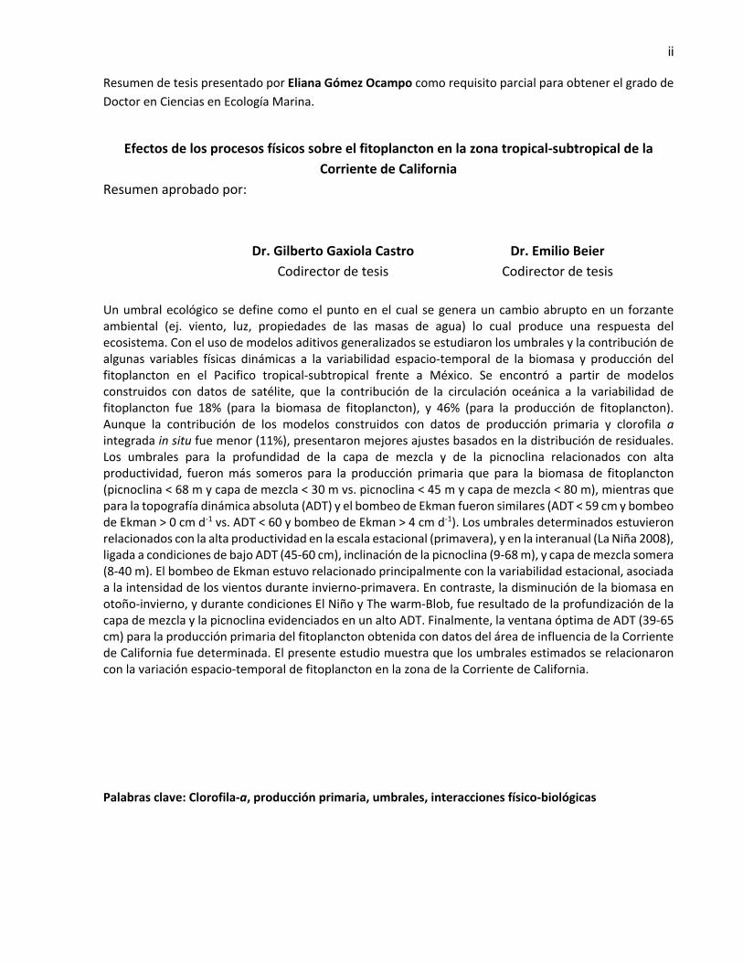
Resumen en español Efectos de los procesos físicos sobre el fitoplancton en la zona tropical‐subtropical de la

Corriente de California

Resumen aprobado por:

________________________ ________________________


Codirector de tesis Codirector de tesis

Un umbral ecológico se define como el punto en el cual se genera un cambio abrupto en un forzante ambiental (ej. viento, luz, propiedades de las masas de agua) lo cual produce una respuesta del ecosistema. Con el uso de modelos aditivos generalizados se estudiaron los umbrales y la contribución de algunas variables físicas dinámicas a la variabilidad espacio‐temporal de la biomasa y producción del fitoplancton en el Pacifico tropical‐subtropical frente a México. Se encontró a partir de modelos construidos con datos de satélite, que la contribución de la circulación oceánica a la variabilidad de fitoplancton fue 18% (para la biomasa de fitoplancton), y 46% (para la producción de fitoplancton). Aunque la contribución de los modelos construidos con datos de producción primaria y clorofila a integrada in situ fue menor (11%), presentaron mejores ajustes basados en la distribución de residuales. Los umbrales para la profundidad de la capa de mezcla y de la picnoclina relacionados con alta productividad, fueron más someros para la producción primaria que para la biomasa de fitoplancton (picnoclina < 68 m y capa de mezcla < 30 m vs. picnoclina < 45 m y capa de mezcla < 80 m), mientras que para la topografía dinámica absoluta (ADT) y el bombeo de Ekman fueron similares (ADT < 59 cm y bombeo de Ekman > 0 cm d‐1 vs. ADT < 60 y bombeo de Ekman > 4 cm d‐1). Los umbrales determinados estuvieron relacionados con la alta productividad en la escala estacional (primavera), y en la interanual (La Niña 2008), ligada a condiciones de bajo ADT (45‐60 cm), inclinación de la picnoclina (9‐68 m), y capa de mezcla somera (8‐40 m). El bombeo de Ekman estuvo relacionado principalmente con la variabilidad estacional, asociada a la intensidad de los vientos durante invierno‐primavera. En contraste, la disminución de la biomasa en otoño‐invierno, y durante condiciones El Niño y The warm‐Blob, fue resultado de la profundización de la capa de mezcla y la picnoclina evidenciados en un alto ADT. Finalmente, la ventana óptima de ADT (39‐65 cm) para la producción primaria del fitoplancton obtenida con datos del área de influencia de la Corriente de California fue determinada. El presente estudio muestra que los umbrales estimados se relacionaron con la variación espacio‐temporal de fitoplancton en la zona de la Corriente de California.

Palabras clave: Clorofila‐a, producción primaria, umbrales, interacciones físico‐biológicas

iii

Abstract of the thesis presented by Eliana Gómez Ocampo as a partial requirement to obtain the Doctor

of Science degree in Marine Ecology.

Resumen en inglés Effects of physical processes on tropical‐subtropical California Current phytoplankton

Resumen aprobado por:

________________________ ________________________


Thesis Co‐director Thesis Co‐director

An ecological threshold, defined as the point at which there is an abrupt change in a quality, property or phenomenon or where small changes in a driver (i.e. wind, light, water masses properties) may produce large responses in the ecosystem. Using generalized additive models the thresholds and the contribution of some dynamic physical variables to phytoplankton production and biomass spatial‐temporal variability were estimated. The results of this work showed from models built with satellite data, that the ocean circulation contribution to phytoplankton variability was 18% and 46% for phytoplankton biomass and phytoplankton production, respectively. Despite of the contribution of the models constructed with in situ integrated chlorophyll‐a and primary production data was lower than with satellite data, based on residual distribution, the fits were better. The pycnocline and mixed layer depths thresholds related to high productivity, were shallower for primary production than those for phytoplankton biomass (pycnocline < 68 m and mixed layer < 30 m vs. pycnocline < 45 m and mixed layer < 80 m), while for absolute dynamic topography (ADT) and Ekman pumping thresholds were similar (ADT < 59 cm and Ekman pumping > 0 cm d‐1 vs. ADT < 60 and Ekman pumping > 4 cm d‐1). The thresholds were related to the high productivity at seasonal (spring), and interannual (La Niña 2008) scales, linked to the generally lower ADT conditions (45‐60 cm), pycnocline sloping (9‐68 m), and shallow mixed layer (8‐40 m). Ekman pumping was mainly related to seasonal variability associated with alongshore wind during winter‐spring strengthening. In contrast, the biomass depletion in autumn‐winter, and during El Niño and Warm‐Blob conditions, was the result of the pycnocline and mixed layer deepening evidenced in high ADT. An optimal ADT window (39‐65 cm) for primary production was estimated with data of the California Current area. The results presented in this study suggest that estimated thresholds are related to the phytoplankton spatial‐temporal variations of the California Current area.

Palabras clave: Chlorophyll‐a, primary production, thresholds, physico‐biological interactions

iv

Dedicatoria

Al Dr. Gilberto Gaxiola Castro “profe Gilo”

(...) Y se dio cuenta de que nadie jamás está solo en el mar…

Ernest Hemingway

v

Agradecimientos

Primero que todo quiero agradecer a mi familia por tener siempre su apoyo incondicional y su amor. Sin

ellos, realizar mis sueños no habría sido posible.

Mis más sinceros agradecimientos al Gobierno mexicano por el financiamiento de mis estudios de

doctorado a través de la beca CONACyT No. 271663. También agradezco el financiamiento parcial de los

proyectos CONACyT No. 236864, 168034‐T y 254745‐T.

Al Centro de Investigación Científica y de Educación Superior de Ensenada, Baja California, (CICESE) por

todos los conocimientos recibidos en el tema de la oceanografía.

Al posgrado en Ecología Marina por admitirme en el programa, apoyarme económicamente para la

asistencia a congresos nacionales e internacionales y otorgarme extensión de beca para culminar mis

estudios.

Agradezco profundamente al Dr. Gilberto Gaxiola Castro, a quien tuve la fortuna de conocer y de que me

acompañara en gran parte de mi camino. Agradezco porque más que un director, se convirtió en mi

mentor, mi apoyo y mi guía. Se convirtió en mi padre académico a través de sus enseñanzas y críticas

constructivas en mi proceso de formación como científica. Nunca olvidaré su apoyo incondicional y la

confianza que siempre depositó en mí y que espero no haber defraudado. Profe, usted solamente nos

abandonó físicamente, su alegría, bondad, calidad humana, entre muchas otras de sus virtudes, siempre

quedarán grabadas en los corazones de las personas que tuvimos la fortuna de tenerlo en nuestro camino.

Siempre lo recordaré como una gran persona e investigador.

A mi comité de tesis agradezco todo el apoyo y los aportes brindados durante este proceso. Al Dr. Emilio

Beier por ayudarme a ingresar al CICESE y por sus buenas ideas. Al Dr. Reginaldo Durazo por sus atinados

aportes en la tesis y por el apoyo brindado en la escritura de los artículos científicos derivados de esta. Al

Dr. Saúl Álvarez por su entusiasmo en compartir sus conocimientos en los cursos del programa Ecología

marina. Al Dr. Enric Pallàs Sanz, por tener la capacidad de traducir la oceanografía física en un lenguaje

fácilmente entendible, para quienes no estudiamos esa área. A la Dra. Elena Solana, por ser la

investigadora que nos brinda a todos los estudiantes de ecología marina, las herramientas necesarias para

el análisis de nuestras tesis a través de los cursos de estadística.

vi

A Gladys Bernal y Vladimir Toro por recibirme y ubicarme en Ensenada.

A mis compañeros de oficina con quienes compartí en estos cinco años: Manuel Mariano (El parcero),

Elizabeth Gahona, Luz María Martínez y Luis Erasmo Miranda. Por los agradables ratos en la oficina y por

siempre tener un buen ambiente de trabajo.

Agradezco al equipo de trabajo del profe Gilo: Martin de la Cruz, Benigno Hernández y Reginaldo Durazo,

por su acogimiento y apoyo.

A Leonardo Tenorio por su cariño, acompañamiento, apoyo y amistad, que hicieron más cálida la estancia

en Ensenada.

A mis amigos más cercanos en Ensenada: Lorena Hernández, Ana Castillo, Cristian Hakspiel, Daniel

Santiago Peláez y Esther Portela. Quienes de alguna u otra manera siempre estuvieron dándome ánimo y

apoyo cuando más lo necesitaba. También agradezco a mis amigos en Colombia, por hacerme sonreír y

acompañarme desde la distancia. Sin ser menos importante, agradezco a la colonia colombiana en

Ensenada (Franklin Muñoz, Laura Echeverri, Javier López, Nereida Moreno, Wencel de la Cruz, Juan Gabriel

Correa y Angélica García) porque con nuestras reuniones sentíamos más de cerca a nuestra amada

Colombia.

A Edgar Josymar Torrejón por nuestras largas conversaciones sobre R, su asesoría en estadística y por su

amistad.

Agradezco a Ania Yarazeth Chamú, Rubén García Guillén y Susan Davies, por hacer más placenteras mis

estancias en La Paz y por abrirme las puertas de su casa.

Agradezco a Elizabeth Farias y a mis compañeros del posgrado en Ecología marina por su

acompañamiento.

En general agradezco a todos aquellos que de una u otra manera aportaron a mi aprendizaje y bienestar

durante estos 5 años.

vii

Table of Contents

Resumen en español ..................................................................................................................................... ii

Resumen en inglés ....................................................................................................................................... iii

Dedicatoria ................................................................................................................................................... iv

Agradecimientos ........................................................................................................................................... v

List of figures ................................................................................................................................................ ix

List of tables ................................................................................................................................................ xii

1. General introduction ..................................................................................................................... 1

1.1 Background .................................................................................................................................... 4

1.2 Significance .................................................................................................................................... 8

1.3 Hypothesis ................................................................................................................................... 10

1.4 Objectives .................................................................................................................................... 11

1.4.1 General objective ................................................................................................................ 11

1.4.2 Specific objectives ............................................................................................................... 11

2. Chapter 2: Approach of dynamic physical thresholds of phytoplankton in tropical‐subtropical Pacific Ocean ................................................................................................................................................. 12

2.1 Introduction ................................................................................................................................. 12

2.2 Methods ...................................................................................................................................... 13

2.2.1 Data sources ........................................................................................................................ 13

2.2.2 GAMs fitting ........................................................................................................................ 15

2.3 Results ......................................................................................................................................... 16

2.3.1 Mean and seasonal spatial patterns ................................................................................... 16

2.3.2 Distribution and relationships between variables .............................................................. 19

2.3.3 Contribution of physical dynamic variables to phytoplankton variability .......................... 22

2.3.1 Thresholds of dynamic physical variables on phytoplankton ............................................. 23

2.3.1 3D structure and phytoplankton variability ........................................................................ 25

2.3.1 Seasonal regional differences ............................................................................................. 25

2.3.2 Interannual patterns related to El Niño/La Niña ................................................................. 27

2.4 Discussion .................................................................................................................................... 31

2.5 Concluding remarks ..................................................................................................................... 36

viii

3. Chapter 3: Effects of the warm anomalies 2013‐2016 on the California Current phytoplankton ... 37

3.1 Introduction ................................................................................................................................. 37

3.2 Methods ...................................................................................................................................... 39

3.2.1 In‐situ data ........................................................................................................................... 39

3.2.2 Satellite data ........................................................................................................................ 40

3.2.3 Statistical Analysis ............................................................................................................... 41

3.2.4 Climate indices .................................................................................................................... 41

3.3 Results ......................................................................................................................................... 42

3.3.1 In‐situ observations ............................................................................................................. 42

3.3.2 2003‐2016 time series ......................................................................................................... 46

3.4 Discussion .................................................................................................................................... 50

3.4.1 "The Blob" and El Niño ........................................................................................................ 50

3.4.2 Trends and climatic indices ................................................................................................. 52

3.4.3 Optimal ADT window for phytoplankton production ......................................................... 55

3.5 Conclusions .................................................................................................................................. 57

4. Chapter 4: General discussion ..................................................................................................... 58

4.1 Shallower mixed layer threshold for PP than for Chla ................................................................ 58

4.2 ADT as a proxy of water column productivity ............................................................................. 59

4.3 Ekman pumping as the dominant forcing of phytoplankton seasonal variability ...................... 60

4.5 Concluding remarks ..................................................................................................................... 61

5. Cited Literature ........................................................................................................................... 62

Annexed ............................................................................................................................................. 69

ix

List of figures

Figure

Page

1

Time series (1998‐2015) in the IMECOCAL Line 100 for: a) pycnocline depth, b) mixed layer depth (MLD), and c) water‐column integrated Chlorophyll‐a. Color points (E30, E35, E40, E45, E50, E55, and E60) are the sampled stations in line 100. Dashed lines indicate the mean values of stations.

2

2

Ecological thresholds for phytoplankton variables. a) Temperature vs. growth rate, b) Sea surface temperature vs. maximum photosynthetic rate (PBopt), d) Nutrient inputs vs. primary production, e) Nutrient inputs vs. Chlorophyll‐a, f) Iron concentration vs. Specific growth rate at high (filled symbols at 500 µE m‐2 s‐1) and low (closed symbols at 50 µE m‐2 s‐1) light conditions, and g) Same as f but Iron vs. Chlorophyll. Figures modified from Eppley (1972) (a), Behrenfeld and Falkowski (1997) (b), Sunda and Huntsman (1997) (c), (d),. and Duarte et al.(2000) (e), (f). ......

5

3

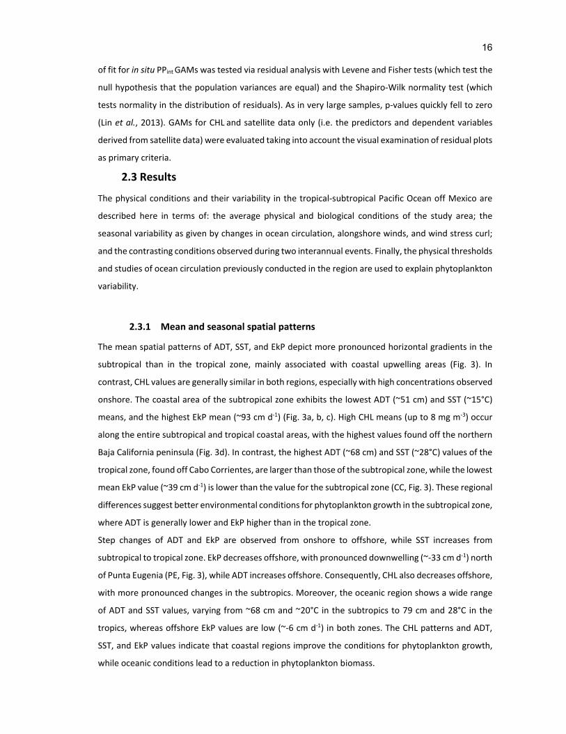
Horizontal distribution of the mean conditions of a) absolute dynamic topography (ADT cm, color contours) and the associated geostrophic velocities (cm s‐1, arrows); b) Ekman pumping (EkP cm d‐1); c) Sea surface temperature (SST °C); and d) Satellite chlorophyll (CHL mg m‐3). In (b), dots indicate the location of hydrographic stations where in‐situ data were collected, while the dashed line indicates the limit between the tropical and subtropical regions at 23.25 °N. Reference points on land for the tropical and subtropical zones are Punta Eugenia (PE) and Cabo Corrientes (CC), respectively. .........................................................................................................

13

4

(a‐d) Seasonal variability of absolute dynamic topography (ADT; cm, color contours) and the geostrophic flow (cm s‐1, arrows), (e‐h) Ekman pumping (EkP; cm d‐1), (i‐l) sea surface temperature (SST; °C), and (m‐p) satellite chlorophyll (mg m‐3) during winter, spring, summer and autumn. ...............................................................

18

5

Box and whisker plots showing differences between the mean, standard error (SE), and range for in situ integrated primary production (PPint, a) and chlorophyll‐a (Chlaint, b), mixed layer depth (MLD, c), pycnocline depth (ZPyc, d), absolute dynamic topography (ADT, e) and Ekman pumping (EkP, f). Wilconxon test results (W and p‐values) are indicated on each plot. ..............................................................

19

6

Relationship between absolute dynamic topography (ADT; a and b) and Ekman pumping (EkP; c and d) with pycnocline depth (ZPyc, a and c) and mixed layer depth (MLD, b and d). Black (gray) points indicate tropical (subtropical) stations, delimited by the 23.5°N latitude, where there were Chlorophyll‐a and primary production measurements ...........................................................................................

20

7

Relationship between integrated water column Chlorophyll‐a (Chlaint; a, c, e, and g), primary production (PPint; c and d) with pycnocline depth (ZPYC, a and b), mixed layer depth (MLD, c and d), absolute dynamic topography (ADT, e and f), and Ekman pumping (EkP, g and h). Black (gray) points indicate tropical (subtropical) stations as delimited by the 23.5 °N latitude. ..............................................................

21

x

8

Results of the generalized additive models (GAMs), illustrating the partial response of the integrated primary production (PPint; a and b) and Chlorophyll‐a (Chlaint; c and d) to the mixed layer depth (MLD, a and c), the pycnocline depth (ZPyc, b and d), Ekman pumping (EkP; e and g), and absolute dynamic topography (ADT; f and h). The smooth functions (s) are represented as solid lines with the 95%‐confidence intervals as shaded areas. Rug lines on the x‐axes represent the observed values of MLD, ZPyc, EkP and ADT. The y‐axis labels show the smooth of the GAMs. The dashed lines represent the threshold values of the change from positive to negative influence of the predictor variable (MLD, ZPyc, EkP, ADT) on the response variable (PPint, Chlaint). The thresholds are specified for each smoothing spline. ...........................................................................................................................

24

9

Seasonal cycle from spring (May 2002; a, b, c, d), autumn (November 2002; e, f, g, h), winter (January 2003; i, j, k, l) and summer (July 2003; m, n, o, p) for absolute dynamic topography (ADT, cm, color contours) and the associated geostrophic flow (cm s‐1, arrows) (a, e, i, m) , Ekman pumping (EkP; cm d‐1) (b, f, j, n), sea surface temperature (SST; °C) (c, g, k, o), and satellite chlorophyll (mg m‐3) (d, h, l, p) . Included are the upper‐layer vertical profiles of temperature (T; °C), potential density (σt, kg m‐3), and Chlorophyll‐a (Chla; mg m‐3) for IMECOCAL subtropical line 100 in spring (q), autumn (s), winter (u) and summer (v), and PROCOMEX tropical line A in spring (r), autumn (t) and summer (w). .........................................................

26

10

Interannual analysis of absolute dynamic topography (ADT color contours) and geostrophic flow (arrows), Ekman pumping (EkP), sea surface temperature (SST) and satellite chlorophyll (CHL) during the extreme El Niño conditions in January 1998 (a‐d) and the extreme La Niña conditions in January 2008 (e‐h). Vertical profiles of temperature (T; °C), potential density (σθ; kg m‐3), and Chlorophyll‐a (Chla; mg m‐3) and its anomalies (Ta, σθa, and Chlaa) for Line 100 IMECOCAL in January 1998 (i) and January 2008 (j) are shown. ........................................................

29

11

Interannual analysis of absolute dynamic topography (ADT color contours) and geostrophic flow (arrows), Ekman pumping (EkP), sea surface temperature (SST) and satellite chlorophyll (CHL) during the extreme El Niño conditions in January 1998 (a‐d) and the extreme La Niña conditions in January 2008 (e‐h). Vertical profiles of temperature (T; °C), potential density (σt; kg m‐3), and Chlorophyll‐a (Chl‐a; mg m‐3) and its anomalies (aT, and aChla) for line 100 IMECOCAL in January 1998 (i) and January 2008 (j) ........................................................................................

30

12

Two scenarios for primary production (PP) and Chlorophyll‐a (Chla) illustrating the thresholds of mixed‐layer depth (MLD), pycnocline depth (ZPyc), absolute dynamic topography (ADT), and Ekman pumping (EkP) that affect phytoplankton production and biomass. Left (right) side corresponds to thresholds that increase (decrease) PP and Chla. Note that arrow size is related to EkP values. The number of microorganisms per water volume represents phytoplankton biomass. ....................

35

13

Area of influence of the California Current System (CCS), divided into geographic zones (northern, central and southern; after Checkley and Barth, 2009). Hydrographic stations are shown as dots (CalCOFI) and triangles (IMECOCAL). .........

37

14 Long‐period average of in‐situ observations (contour lines) in summer (August) temperature (T), salinity (S), and Chlorophyll‐a (Chl‐a) and standardized anomalies

42

xi

(colors) in the summer 2014 (aT, aS, aChl‐a) for the hydrographic lines of CalCOFI a) line 76.7, b) line 87.7, and c) line 93.3) and IMECOCAL programs d) line 100, e) line 120, and f) line 130). Color bars represent anomaly ranges (up to down) for Ta, Sa and Chl‐a a. .......................................................................................

15

Summer (August) long‐period average for: a) Sea surface temperature (SST), b) Absolute dynamic topography (ADT) and geostrophic velocity (vectors), c) Satellite chlorophyll (CHL), d) model primary production (PP). The polygons in panel (a) show the division in southern (SZ), transitional (TZ), central (CZ) and northern (NZ) zones. The polygons in panel (a) show the division in southern (SZ), transitional (TZ), central (CZ) and northern (NZ) zones. ..................................................................

44

16

Anomalies for 2014 in the CC zone for a) Sea surface temperature (SST), b) Absolute dynamic topography (ADT), c) satellite chlorophyll (CHL), d) model primary production (PP). ..............................................................................................

45

17 Same as figure 14 for 2015. ..........................................................................................

46

18

Monthly time series (2003‐2016) in the CC north (left panel) and central zones (rigth panel) for: sea surface temperature (SST, a, e; °C), absolute dynamic topography (ADT, b, f; cm), satellital chlorophyll (CHL, c, g; mg m‐3), and primary production (PP, d, h; gC m‐2 d‐1). Black line represents the running average (12 months) for each data point. Dashed lines indicate the warm Blob in 2013 and 2016 El Niño. The horizontal dashed line in CHL and PP indicates the trend significant in a pvalue < 0.05. Only the trends with slope > 0.001 are shown. ............

47

19 Same as Figure 17, for the transitional and south CC zones. .......................................

48

20

Time series (2003‐2016) in the CC northern (a, c and e) and central zones (b, d and f) for: Sea surface temperature anomalies (SSTa; a, b; °C), satellital chlorophyll anomalies (CHLa; c, d; mg m‐3), and primary production anomalies (PPa; e, f; gC m‐2 d‐1). Red bars denote the positive anomalies, while blue bars represents the negative anomalies. Dashed lines indicate the warm Blob in 2013 and 2016 El Niño.

49

21 Same as figure 8 but transitional (a, c, and e) and south zones (b, d, and f). ..............

50

22 Climatic indices: a) Pacific Decadal Oscillation (PDO), b) North Pacific Gyre Oscillation (NPGO), .......................................................................................................

52

23

Results of the Generalized Additive Model (GAM) functions, illustrating the partial response of integrated PP to Absolute Dynamic Topography (ADT). The smooth function (solid line) with 95% confidence interval (shaded area are shown for the predictor variable). Rug lines on the x‐axis represent the values observed. Labels on the y‐axis show the effective degrees of freedom for the smooth terms of GAMs. Vertical dashed lines limit the range of ADT values for which positive effects on PP were observed. ...................................................................................................

56

xii

List of tables

Table Page

1 Correlation matrix (pairwise Pearson correlation coefficients) of the predictor

variables absolute dynamic topography (ADT), Ekman pumping (EkP), mixed layer

depth (MLD), and pycnocline depth (ZPyc). All correlations were significant at p <

0.001. .............................................................................................................................

22

2 Alternative generalized additive models for primary production (PPint) and Chlaint as

a function of the predictor variables absolute dynamic topography (ADT), Ekman

pumping (EkP), mixed layer depth (MLD, and pycnocline depth (ZPyc). EkP is the one‐

week average at the time of sampling while EkP1 and EkP2 are averages over one and

two weeks before sampling, respectively. The smooth functions are represented by

s, n is the number of samples used to produce the respective predictive model, %D2

is the percentage of explained deviance, AIC refers to the Akaike Information

Criterion, Ft, Lt, and ShWt are the p‐values for Fisher, Levene, and Shapiro‐Wilks test,

Xr refers to residuals averaged and Corr is the correlation coefficient between

observed and predicted data. All smooth terms were significant (all p‐values < 0.001).

The models are listed from the lowest to the highest AIC. The best‐fitting models

based on the residual distribution are highlighted in grey. As Chlaint n is high and thus

p‐values go to infinite, the residuals were visually evaluated as bad (‐), regular (‐‐),

good (‐‐‐) in Rd column. .................................................................................................

23

3 Alternative generalized additive models for model primary production (PPm) and

satellite chlorophyll (CHL) as a function of the predictor variables absolute dynamic

topography (ADT), and Ekman pumping (EkP). The smooth functions are represented

by s, n is the number of samples used to produce the respective predictive model,

%D2 is the percentage of explained deviance, AIC refers to the Akaike Information

Criterion, Rd is residual distribution classified as bad (‐), regular (‐‐), good (‐‐‐), Xr

refers to residuals averaged and Corr is the correlation coefficient between observed

and predicted data. All smooth terms were significant (all p‐values < 0.001). The

models are listed from the lowest to the highest AIC. The best‐fitting models based

on the residual distribution are highlighted in grey. .....................................................

23

4 Physical (ZPyc, pycnocline depth; MLD, mixed layer depth; Zeu, euphotic zone depth;

ADT, absolute dynamic topography, and EkP, Ekman pumping) and biological

variables (Chlaint, Chlorophyll‐a, and PPint, primary production, both integrated in

water column) for some analyzed stations (St, Station; Yr, year; M, month) in Fig 8‐9.

.......................................................................................................................................

32

1

1. General introduction

Phytoplankton represent the first trophic level and is a key component of the epipelagic

ecosystem. Moreover, as a result of the photosynthesis processes it plays a key role in the ocean

carbon biological pump as atmospheric CO2 remover. The distribution and phytoplankton

growth is limited to the euphotic zone through the availability of light and nutrients, which are

mainly driven by the ocean circulation, including up‐and‐down pycnocline movements, mixed‐

layer dynamics, and upwelling. Phytoplankton size structure largely determines the trophic

organization of pelagic ecosystems and thus the efficiency with which organic matter produced

by photosynthesis is channeled towards upper trophic levels or exported to the ocean’s interior

(Falkowski and Oliver, 2007).

Most of the studies about the relationship between marine phytoplankton and circulation‐

driven physical processes rely on understanding the effects of those processes more than on

defining the ecological thresholds in which the variables involved affect the microorganisms. The

concept of ecological thresholds emerged in the 1970’s from the idea that ecosystems often

exhibit multiple ‘‘stable’’ states, depending on environmental conditions (Holling, 1973; Beisner

et al., 2003). An ecological threshold, defined as the point at which there is an abrupt change in

a quality, property or phenomenon or where small changes in a driver (i.e. wind, light, water

masses properties) may produce large responses in the ecosystem (Groffman et al., 2006) .

Ecological discontinuities imply critical values of the independent variable around which the

system flips from one stable state to another, that is, ecological thresholds (Muradian, 2001).

The peninsula off Baja California has experienced the influence of large‐scale processes affecting

phytoplankton growth. The in situ sampling made by the IMECOCAL program (Investigaciones

Mexicanas de la Corriente de California, spanish acronym) has allowed monitoring physical and

biological variables changes since 1997. Both mixed layer and pycnocline depth, and the

integrated Chlorophyll‐a (Chla), have exhibited changes in their values throughout the time

series for Line 100 of IMECOCAL (Fig. 1). Some studies (Lavaniegos et al., 2002; Gaxiola‐Castro,

2010; Espinosa‐Carreón et al., 2015) have correlated these changes with ocean circulation

changes produced by ENSO (El Niño Southern Oscillation) cycles and fluctuations in California

Current intensity (i.e., Subarctic Water intrusion in 2002‐2006). Few studies (Gaxiola‐Castro,

2010; Espinosa‐Carreon et al., 2012; Espinosa‐Carreón et al., 2015) combined the analysis of

physical dynamic variability, associated to ocean circulation, with biological data to address

phytoplankton varibility.

2

The deepening of the mixed layer causes phytoplankton concentrations to further decrease

(rather than increase) because the slowly accumulating population is being distributed over an

increasing volume of water (i.e., being diluted) (Banse, 1982; Backhaus et al., 2003; Ward and

Waniek, 2007; Behrenfeld, 2010; Behrenfeld and Boss, 2014). Moreover, if phytoplankton cells

change their light depth through vertical movements associated with turbulence, they

photosynthesize according to the trajectory of the photosynthesis‐light or photosynthesis‐depth

relationship. Pycnocline depth (ZPyc) is directly related to nutrients availability in the euphotic

zone. Vertical flux of nutrients from the pycnocline is a key factor which supplies phytoplankton

Figure 1 Time series (1998‐2015) in the IMECOCAL Line 100 for: a) pycnocline depth, b) mixed layer depth

(MLD), and c) water‐column integrated Chlorophyll‐a. Color points (E30, E35, E40, E45, E50, E55, and E60)

are the sampled stations in line 100. Dashed lines indicate the mean values of stations.

3

growth and supports new production (Yunev et al., 2005). Despite our knowledge of the effects

of mixed layer (Marra, 1978; Polovina et al., 1995; Behrenfeld and Boss, 2014) and pycnocline

dynamics on phytoplankton, the thresholds in which these variables affect phytoplankton

remain unclear.

In order to better understand the phytoplankton spatial response to ocean circulation processes

at different temporal scales: months (related to seasonal circulation), and interannual (related

to El Niño/La Niña Southern Oscillation cycle and The warm Blob), in this work the following

questions were answered:

1) Is there a common threshold of dynamic physical variables related to ocean circulation

that explains phytoplankton changes at the seasonal and interannual scales?

2) How much does the contribution of ocean circulation account for phytoplankton

variability?

In order to respond the latter questions, some particular cases are presented and explored, as

follows:

In Chapter 2, the phytoplankton response at different scales in the subtropical‐tropical

Pacific off Mexico were studied. For the seasonal scale, January 2003 for winter, May

2002 for spring, July 2003 for summer, and November 2002 for autumn datasets were

selected. For the interannual scale, two contrasting time periods are used: January 1998

and 2008.

In Chapter 3, the effects of “The Warm Blob 2013‐2014,” and “2015‐2016 the El Niño”

on phytoplankton in the California Current were analyzed.

In both chapters, an explanation of the phytoplankton response to the water column structure

and the surface ocean conditions is given. In chapter 2, the relationship between in situ depth‐

integrated primary production (PPint), Chlorophyll‐a (Chla; as a proxy for phytoplankton biomass)

and CTD derived‐data (Mixed layer depth (MLD) and ZPyc), as well as satellite‐derived absolute

dynamic topography (ADT), Ekman pumping (EkP) (as proxies for ocean circulation patterns),

satellite derived sea surface temperature (SST), and satellite chlorophyll (CHL, in capital letters

to differentiate it from in situ Chla) over subtropical‐tropical Pacific off Mexico was analyzed.

We used ADT, SST, EkP, and CHL data to capture the snapshot of surface conditions, and then

an exploration was made inside the water column through the vertical profiles of temperature,

potential density, and Chla. In chapter 3, in situ data from IMECOCAL and CALCOFI programs

were analyzed, in order to estimate the temperature, salinity, and Chla anomalies together with

satellite data of ADT, SST, CHL, and modeled primary production (PPm) in the CCS. To estimate

the contribution of ocean circulation to phytoplankton production and biomass variability, and

the thresholds in physical variables that explain phytoplankton response at different spatial‐

temporal scales, generalized additive models (GAMs) (Hastie and Tibshirani, 1986) were used.

4

In chapter 2, the thresholds of ZPyc, MLD, ADT, and EkP in which phytoplankton changes abruptly

were estimated using GAMS built from both in situ and satellite data. In chapter 3, a larger region

of that covered in chapter 2 was considered, which allowed for the estimation of ADT and SST

values over a larger spatial scale, and the thresholds within which they affect primary

production. Finally, in chapter 4 a general discussion of the main results is presented.

1.1 Background

Over the last four decades, some studies have determined thresholds of several variables

affecting phytoplankton organisms. For example Eppley (1972) determined that the maximum

expected phytoplankton growth rate occurred for temperatures less than 40 ºC (Fig. 2a).

Behrenfeld and Falkowski (1997) estimated that the median of maximum photosynthetic rate,

was the lowest at temperatures < l ºC and increased rapidly between 1 ºC and 20 ºC (Fig. 2b).

Duarte et al. (2000) studied the response of the biomass and primary production of

phytoplankton community to a gradient of nutrient inputs in a large‐scale mesocosm nutrient

enrichment experiment. They found that the community biomass increased to a maximum of

40.8 µg Chlorophyll‐a L‐1 (200‐fold above the mean initial value) and primary production reached

a level 10‐fold higher at the highest nutrient loading (5 µM d‐1) than at the normal loading rate

(Fig. 2 c and d). Also, Sunda and Huntsman (1997) determined that the amount of cellular iron

needed to support growth is higher under lower light intensities. Phytoplankton growth can

therefore be simultaneously limited by the availability of both iron and light (Fig. 2 e and f). The

latter variables are much known for explaining phytoplankton distribution in the oceans, and

they have the advantage that can be studied by means of laboratory cultures and mesocosm

experiments. However, in the real world, the phytoplankton habitat is a dynamic environment,

which is driven by physical processes affecting its growth, and where other dynamic physical

variables, which can be a hard task control experimentally, take place.

5

Figure 2 Ecological thresholds for phytoplankton variables. a) Temperature vs. growth rate, b) Sea surface

temperature vs. maximum photosynthetic rate (PBopt), d) Nutrient inputs vs. primary production, e)

Nutrient inputs vs. Chlorophyll‐a, f) Iron concentration vs. Specific growth rate at high (filled symbols at

500 µE m‐2 s‐1) and low (closed symbols at 50 µE m‐2 s‐1) light conditions, and g) Same as f but Iron vs.

Chlorophyll. Figures modified from Eppley (1972) (a), Behrenfeld and Falkowski (1997) (b), Sunda and

Huntsman (1997) (c), (d),. and Duarte et al.(2000) (e), (f).

Physical processes have an important role supporting productivity in the ocean. The

characteristic time and space scales for open ocean motions are from weeks to several years

and from tens of meters to thousands of kilometers. Despite the spatial‐temporal differences in

which the physical processes occur, they have in common that allow the uplift and subduct of

nutrient‐rich isopycnal surfaces into the euphotic zone. Therefore, these physical processes that

make nutrients available to phytoplankton are relevant to study in several scales, such as

mesoscale related to eddies, seasonal related to coastal upwelling, and interannual related to

6

ocean circulation variability. Thus, the understanding of the physical variations of phytoplankton

habitat, helps to explain variations in marine ecosystems.

Mesoscale physical phenomena have long been thought to influence phytoplankton through the

horizontal advection of water masses and/or their influence on net vertical transport. Eddies

influence biogeochemical stocks and rates by horizontal advection and lateral stirring of water

masses, the tilting of isopycnal surfaces enabling vertical transport by isopycnal mixing, and the

uplift of nutrient‐rich isopycnal surfaces into the euphotic zone (Siegel et al., 1999). McGillicuddy

et al. (2007) observed at least three types of mid‐ocean eddies in the northwestern subtropical

Atlantic: cyclones, anticyclones, and mode‐water eddies. Cyclones dome both the seasonal and

main pycnocline, whereas regular anticyclones depress both density interfaces. Mode‐water

eddies derive their name from the thick lens of water that deepens the main pycnocline while

shoaling the seasonal pycnocline. Because the geostrophic velocities are dominated by

depression of the main pycnocline, the direction of rotation in mode‐water eddies is the same

as in regular anticyclones. However, displacement of the seasonal pycnocline is the same as in

cyclones: Both types of features tend to upwell nutrients into the euphotic zone during their

formation and intensification phases. As these eddies spin down, the density surfaces relax back

to their mean positions, and thus decaying cyclones and mode‐water eddies will have

downwelling in their interiors. Therefore, there are several types of mesoscale eddies that lift

nutrient‐replete isopycnals into the euphotic zone, where those nutrients are rapidly utilized by

phytoplankton.

Coastal upwelling is the main seasonal scale mechanism that enhances ecosystem productivity.

It is one of the dominant forcing agents produced by favorable wind stress. The offshore Ekman

transport produced when winds blow alongshore, shifts the location of the thermocline due to

vertical pumping, and increases the phytoplankton productivity through the nutrients

availability in the euphotic zone. Although, in some coastal regions the occurrence of coastal

upwelling is given by the winds seasonality, some strong interannual climate forcing events have

had influence in its variability. For example, during 1999 La Niña the strongest coastal upwelling

of the last 54 years took place in the CCS (Hayward et al., 1999). Also, in 2005 atmospheric

forcing anomalies lead to a coastal upwelling delay of 2–3 months in the northern CCS and

created a significant perturbation in ocean conditions and the marine ecosystem (Schwing et al.,

2006). In 2014 as a consequence of “The warm Blob”, the CCS (~28˚–48˚N) exhibited average, or

below average, coastal upwelling and relatively low productivity in most locations (Leising et al.,

2015). Thus, the study of coastal upwelling influence on phytoplankton production and biomass

is key for understanding the marine ecosystem variability.

Interannual climate forcing events produce changes in physical conditions of phytoplankton

habitat. One of the most known interannual events is the ENSO cycle. This climate forcing causes

7

changes in atmospheric and ocean circulation patterns in the Pacific Ocean, which drive to

anomalous winds and changes in thermocline depth. The anomalous warming of the equatorial

Pacific observed during El Niño is propagated from the western Pacific to the eastern boundary

currents as an equatorial Kelvin wave, deepening the thermocline and raising sea level (Huyer

and Smith, 1985). During the 1997‐1998 El Niño, surface nitrate was 21% below average and

new production was reduced by 70%, with deleterious effects on zooplankton, fish, marine

mammals, and seabirds in the CCS (Chavez et al., 2002). Moreover, other atypical interannual

event, the “The warm Blob” (2013‐2014), caused by anomalous distribution of sea level

atmospheric pressure over the eastern North Pacific, produced lower than normal rates of loss

of heat from the ocean to the atmosphere, heated the upper ocean (Bond et al., 2015) and

consequently phytoplankton biomass declined (Leising et al., 2015) . Therefore, climate forcing

events that occur at large spatial‐temporal scales, alter atmospheric and oceanic circulation

patterns, which in turn, produce changes in key dynamic physical variables which limit

phytoplankton growth at regional scales.

There are few studies that estimate the thresholds of dynamic physical variables limiting

phytoplankton growth at different spatial‐temporal scales. The MLD is perhaps the physical

variable more studied for its effect on phytoplankton. However, most studies are focused on

analyzing the change in photosynthesis over time at various irradiance levels or depths (Marra,

1978; Gardner et al., 1995), more than on defining thresholds in which mixed layer depth affects

phytoplankton. Some studies have found that the Chla maximum is centered at MLD ~50 m as

in the Arabian Sea (Gardner et al., 1999). Other studies have focused on how MLD changes

impact phytoplankton concentrations. For example, Behrenfeld and Boss (2014) observed

differences between changes in chlorophyll concentrations and mixed‐layer‐integrated

chlorophyll with changes in MLD. A 50% decrease in MLD results in the same final chlorophyll

concentration as the initial state, but integrated chlorophyll decreases. Doubling the MLD dilutes

the accumulating phytoplankton population such that the final concentration decreases, but

integrated chlorophyll increases. However, MLD is not the only dynamic physical variable

affecting phytoplankton distribution. There are other physical variables as ZPyc, dynamic heigh

(as ADT), and wind‐driven variables known for establishing the physical conditions of

phytoplankton habitat (McGillicuddy et al., 2007; Klein and Lapeyre, 2009).

Despite the fact that ZPyc, ADT, and wind‐driven variables are widely known to influence

phytoplankton distribution, the literature only describes their effects and relationships with

phytoplankton. For example, in the Bering Sea wind mixing, and temperature below the

pycnocline explained 85% of Chla variability (Eisner et al., 2015). Espinosa‐Carreón et al. (2012)

found an inverse relationship between sea surface height and CHL (r =0.83; p < 0.05) in the same

area of this work. Although, the latter and related studies have been important to explain the

8

phytoplankton distribution, the thresholds in which phytoplankton growth is affected, could be

a useful tool to understand variations in phytoplankton and other trophic levels, when having

measurements and remote sensing data of the dynamic physical variables of the habitats.

Some approximations of physical dynamic thresholds have been estimated for other organisms.

Asch and Checkley (2013) found that the greatest probability of encountering anchovy, sardine,

and jack mackerel eggs occurred at dynamic heights of 79–83 cm, 84–89 cm, and 89–99 cm,

respectively. Optimum habitats at absolute dynamic topography values of 48.7 to 50.7 cm for

blue whales and 43.7 to 50.7 cm for short‐beaked common dolphins were estimated by Pardo

et al. (2015). Similar studies are necessary for phytoplankton organisms, and its importance will

be pointed out in the next section.

1.2 Significance

The CCS is influenced by different atmospheric climate stressors; it is mainly affected by large‐

scale change patterns in atmospheric pressure (Checkley and Barth, 2009). The phytoplankton

in this area is directly impacted by phenomena at different scales imposed by climate variability.

For example, during the 1997‐1998 El Niño event, phytoplankton biomass and production

dropped drastically (Lynn et al., 1998). During 1998‐1999, the cold conditions of the ocean that

resulted from a moderate La Niña event in 1999 derived from anomalous atmospheric stressors,

and led, as mentioned above, to the strongest coastal upwelling recorded in the past 54 years

in the CCS (Schwing et al., 2000), which also produced a shallow nutricline in the tropical coastal

region off the Mexican coast (Lara‐Lara and Bazán‐Guzmán, 2005), as well as high phytoplankton

production and biomass in the CCS (Hayward et al., 1999). On the other hand, the marine

ecosystem off the Baja California peninsula experienced the unusual presence of cold Subarctic

water, which was detected in the summer of 2002 (Durazo et al., 2005a), but became more

evident in the autumn (Gaxiola‐Castro et al., 2008), and its influence ended in 2006 (Durazo,

2009). The response of phytoplankton was evident, with negative Chla anomalies across the

water column (Gaxiola‐Castro et al., 2008) and the drop in primary production (Espinosa‐

Carreón et al., 2015). In the winter of 2013‐2014, sea surface temperature records showed

anomalous positive values (Bond et al., 2015) from Baja California to Alaska. Besides the “Warm

Blob,” at the beginning of the summer of 2015, a weak‐to‐moderate El Niño led to an above‐

average sea surface temperature across the Equatorial Pacific (http://www.elnino.noaa.gov/).

According to the March and April 2016 NOAA report, El Niño occurred with a greater intensity

during the 2015‐2016 winter‐spring in the Northern Hemisphere, shifting to a neutral ENSO (El

Niño/Southern Oscillation) during the late spring ‐ early summer of 2016

(http://www.elnino.noaa.gov/). The direct influence of the different climate variability scales on

9

the CCS, and the ocean circulation complexity of the area, makes this ocean region very suitable

for understanding the large to mesoscale response of phytoplankton to physical stressors. A

sound understanding of the relation between circulation‐driven physical processes and

phytoplankton production and biomass in the epipelagic zones of the ocean is essential to

understand how future circulation changes may modify phytoplankton distribution.

Highly productive areas in the ocean are the result of a continuous nutrient input following

pycnocline shoaling due to: mesoscale cyclonic circulation (Falkowski et al., 1991), and

outcropping due to wind‐driven upwelling and seasonal fronts (McGillicuddy and Robinson,

1997; Klein et al., 2005). The upwelling of cold sub‐surface water during, the formation or

intensification of cyclonic eddies and coastal upwelling, results in a reduction of the total volume

of the water column above the pycnocline due to the higher sea water density, which in turn

reduces the ADT (Rebert et al., 1985). As a result, the nutrient‐rich waters are lifted into the

euphotic zone enhancing biological production (Daly and Smith, 1993). Opposite conditions

occur when warm surface water occupies the surface layer. Consequently, the horizontal surface

ADT gradients reflect the pycnocline vertical movement (Rebert et al., 1985) and can be directly

linked to water‐column productivity. Wind‐driven divergence of the Ekman transport produced

by wind stress curl induces Ekman pumping (EkP), which is among the most important wind

stress driven mechanisms on the sea surface, enhancing biological production through the

transport of nutrients to the euphotic zone (Siegel et al., 1999; McGillicuddy et al., 2007; Gaube

et al., 2013). A positive and intense EkP induces upwelling of sub‐surface water enhancing

productivity, whereas negative EkP presses the nutrient‐rich water below the euphotic zone

resulting in poor productivity. EkP velocities are thus representative for the water‐column

physical conditions that directly affect phytoplankton production and biomass. Therefore, ADT

and EkP are high spatial‐temporal resolution variables associated to ocean circulation and ‐

pycnocline movements‐ which can be proxies of high (low) productive (poor) areas in the ocean.

The pycnocline is also an ecological boundary because it may include a physiological

temperature limit and because it often corresponds to gradients in nutrients, oxygen, or other

limiting factors. Over the last ~50 years, the pycnocline has deepened by 5 m in the CCS, but

showed little net change in stratification, which weakened by 5% in the mid‐1970s, strengthened

by 8% in the mid‐1990s, and then weakened by 4% in 2008 (Fiedler et al., 2013). Significant

increase in net primary production and Chla annual peak levels, i.e., the ‘‘bloom magnitude,’’

were found along the coasts of the CCS for the period of modern ocean color data (1997–2007)

(Kahru et al., 2009). However, it is not clear what specific mechanism is driving the patterns of

increased biomass during this period. Therefore, studies combining physical and biological

variables are necessary for answering the remaining questions.

10

The big problem in ecological research is the availability of in situ data for understanding the

relationships between the organisms and the environment. Remote sensing has helped to

monitor various aspects in ocean conditions which limit the species distributions. However,

satellite data should be validated with in situ information. The subtropical zone of the North

Eastern Pacific has been studied by different monitoring programs such as CalCOFI (California

Cooperative Oceanic Fisheries Investigations) and IMECOCAL. Moreover, other programs as

PROCOMEX (Programa de la Corriente Costera Mexicana, Spanish acronym) and ISFOBAC

(Investigaciones del Sistema frontal de Baja California, Spanish acronym) made biological and

physical sampling of the tropical Pacific Ocean off Mexico. Thus, the availability of in situ data in

the CCS, together with satellite data, plus the complex ocean circulation patterns, make of this

a suitable region for studying physical‐biological interactions between phytoplankton and its

environment. The link between variables derived of in situ measurements, such as primary

production, Chla, pycnocline and mixed layer depth, with variables obtained from remote

sensing, as ADT and EkP, will allow us to provide high spatial‐temporal resolution proxies of

water column productivity, through the estimations of physical thresholds limiting

phytoplankton growth.

As phytoplankton is the base of the epipelagic ecosystem, this contribution will have relevance

in studies of phytoplankton and other trophic levels. Thus, the hypothesis and objectives that

are addressed in this work are detailed next.

1.3 Hypothesis

Two questions, from which two hypothesis are linked, are proposed:

There is a common threshold of ADT, EkP, MLD and ZPyc in which phytoplankton

production and biomass have an abrupt change in seasonal, and interannual scales. The

lowest ADT, MLD and ZPyc values will be related to the highest production and biomass,

and similarly for positive EkP. In contrast, the opposite conditions of ADT, MLD, ZPyc, and

EkP, will be related to the lowest values of primary production and biomass. These

relationships will be not linear and will help to understand the distribution of

phytoplankton and biomass at different variability scales.

The physical dynamic variables related to ocean circulation will reproduce a non‐

negligible percentage of likelihood of phytoplankton production and biomass values.

11

1.4 Objectives

1.4.1 General objective

To understand phytoplankton production and biomass variations in the California Current

System related to physical dynamic variables thresholds.

1.4.2 Specific objectives

By using GAMs, to estimate the thresholds of ZPyc, MLD, ADT and EkPfor the water

column integrated phytoplankton production and biomass.

Using the GAMs estimated thresholds of the physical dynamic variables, to understand

the spatial‐temporal phytoplankton variations in the seasonal and interannual scales

with the GAMs estimated thresholds of the physical dynamic variables.

To determine trends in phytoplankton biomass and production in the California Current

System, and its relationship with large scale processes, for the period 2003‐2016.

The abstract of the manuscript submitted to Journal of Geophysical Research – Biogeosciences (at February 2017, under review) related to this chapter, is

found in appendix section.

12

2. Chapter 2: Approach of dynamic physical thresholds of

phytoplankton in tropical‐subtropical Pacific Ocean

2.1 Introduction

The understanding and scientific assessment of oceanic environmental condition thresholds help to

understand the functioning of ecosystems. This is particularly useful at the first trophic level, where

phytoplankton is a key component of epipelagic ocean productivity. However, most research on the

relationship between marine phytoplankton and circulation‐driven processes has relied on

understanding the effects of those processes rather than defining the ecological thresholds at which

the variables involved affect microorganisms (McGillicuddy and Robinson, 1997; Siegel et al., 1999;

Espinosa‐Carreon et al., 2012). The vertical distribution of phytoplankton is limited to the euphotic

zone through the availability of light and nutrients, which are mainly driven by physical processes

related to ocean circulation, including up and down pycnocline movements, mixed‐layer dynamics,

and upwelling (Behrenfeld et al., 2006). As a result of photosynthetic processes, phytoplankton plays

a key role in the ocean biological carbon pump as removers of atmospheric CO2.

The objective of the present study is to estimate the ZPyc, MLD, ADT, and EkP thresholds that help to

understand phytoplankton biomass and production variations patterns observed on seasonal and

interannual scales. The tropical‐subtropical transitional region of the northeast Pacific off Mexico was

selected for this study (Fig. 3). The transition is defined by the equatorward‐flowing California Current

in spring and summer, and by tropical water masses from the poleward‐flowing Mexican Coastal

Current during summer and autumn. The region is dynamically influenced by coastal upwelling,

upwelling fronts, and complex structures such as meanders, eddies, filaments, and jets (Lynn and

Simpson, 1987; Chelton et al., 2011; Kurczyn et al., 2012; Durazo, 2015). This study relates changes in

the physical variables of the circulation‐driven processes to the spatial response of phytoplankton on

different temporal scales ‐ both monthly (related to seasonal circulation) and interannual (related to

the ENSO cycle). Both satellite‐derived and in situ data were used to capture snapshots of the surface

and water column conditions, respectively. GAMs were used to understand phytoplankton biomass

and production on the aforementioned temporal scales. The aim was to statistically estimate the

thresholds of key dynamic physical variables of ocean circulation that limit phytoplankton growth on

several temporal scales. The advantage of this study is that the variables used integrate the three‐

dimensionality of ocean circulation that affects phytoplankton biomass and production response with

wide spatial‐temporal coverage and high horizontal resolution.

13

2.2 Methods

2.2.1 Data sources

From 1998 throughout 2012, a total of 18,635 Chla (mg m‐3) samples were taken, on board, from five

depths (1, 10, 20, 50, and 100 m) at oceanographic stations in the Pacific Ocean off Mexico (Fig. 3).

Water samples were filtered using Whatman GF/F filters with Chla determined via the fluorescence

method (Yentsch and Menzel, 1963; Holm‐Hansen et al., 1965) described by Venrick and Hayward

[1984]. Primary production (PP; mgC m‐3 h‐1) was determined with 14C incubations (Steeman‐Nielsen,

1952) in situ (~2 hours), with samples collected at six irradiance levels (100%, 50%, 30%, 20%, 10%,

and 1% of surface irradiance), at 470 hydrographic stations. Both biological variables were vertically

integrated using the trapezoidal rule to obtain Chlaint (mg m‐2) from the surface to a depth of 100m,

and PPint (gC m‐2 d‐1) from the surface to the depth corresponding to 1% of surface irradiance.

At each station, CTD casts were conducted using a factory‐calibrated SBE 911 plus profiler. In

accordance with Jeronimo and Gomez‐Valdes (2010), temperature and salinity recorded by the CTD

were used to delimit the mixed layer depth (MLD). They defined MLD as the vertical distance from a

Figure 3. Horizontal distribution of the mean conditions of a) absolute dynamic topography (ADT cm, color

contours) and the associated geostrophic velocities (cm s‐1, arrows); b) Ekman pumping (EkP cm d‐1); c)

Sea surface temperature (SST °C); and d) Satellite chlorophyll (CHL mg m‐3). In (b), dots indicate the

location of hydrographic stations where in‐situ data were collected, while the dashed line indicates the

limit between the tropical and subtropical regions at 23.25 °N. Reference points on land for the tropical

and subtropical zones are Punta Eugenia (PE) and Cabo Corrientes (CC), respectively.

14

reference level in the quasi‐isopycnal layer to the level where density has changed by a fixed∆

∆ , , , , , where θ is potential temperature, S is salinity, P is pressure at the

sea surface, and Δθ and∆ are the potential temperature and potential density increments,

respectively. They estimated the time‐dependent optimal values of Δθ as 0.2°C, 0.5°C and 0.8°C. These

values were taken at the northeast region (latitude >23.5°N) for April, July, and October to January,

respectively. For regions south of 23.5°N, where there are no reports of Δθ optimal values, the value

0.8°C was taken as proposed by Kara et al. [2000]. The pycnocline depth was calculated as the midpoint

depth of a line segment with a maximum slope (‐dT/dz) in the temperature profile, between any two

temperature observations with dz=10 m (Fiedler et al., 2013).

This study used monthly composite imagery of SST and CHL from the Moderate Resolution Imaging

Spectroradiometer (MODIS‐Aqua) sensor with a spatial resolution of 4 km, for the period 2002‐2012.

SST was obtained from the Advanced Very High Resolution Radiometer (AVHRR) sensor

(http://data.nodc.noaa.gov), and CHL was from Sea‐Viewing Wide Field‐of‐View Sensor (SeaWiFS)

(http://oceandata.sci.gsfc.nasa.gov) for periods earlier than June 2002. Modeled primary production

data (PPm, 9×9 km) was derived from the SeaWiFS CHL data using Behrenfeld and Falkowski’s [1997]

Vertical Generalized Production Model (VGPM) (https://coastwatch.pfeg.noaa.gov). Daily absolute

dynamic topography (ADT, cm) maps and associated geostrophic velocities (cm s‐1) were obtained for

1998 to 2012 in a 0.25º×0.25º regular grid from the Archiving Validation and Interpretation of Satellite

Oceanographic Data (AVISO, http://www.aviso.oceanobs.com) program.

The linear Ekman pumping velocity (EkP, cm d‐1) was calculated from the wind stress curl [Gill, 1982]

using sea surface wind data ( reference level of 10 m) provided by the Cross‐Calibrated Multi‐Platform

(CCMP) project at the Physical Oceanography Distributed Active Archive Center (PODAAC;

http://podaac.jpl.nasa.gov/). The data was provided at high temporal (6‐hourly) and spatial (0.25º ×

0.25º) resolutions for the period 1997 to 2010. Wind stress was calculated according to Trenberth et

al.(1990).

ADT was averaged over one‐week intervals at the time of sampling, for statistical analysis. The average

EkP was calculated over one week preceding phytoplankton sampling, as these periods typically

represent the time‐lag between the input of nutrients to the euphotic zone and the corresponding

phytoplankton growth (Marañón et al., 2012; Xie et al., 2015). ADT and EkP data were then paired to

the in situ phytoplankton variables at the closest location and time. This selection procedure produced

a final dataset of: 1) integrated in situ euphotic‐zone phytoplankton production (PPint); 2) depth‐

integrated in situ chlorophyll (Chlaint); 3) MLD; 4) ZPyc; 5) satellite‐derived weekly ADT taken at the time

of phytoplankton sampling; and, 6) satellite wind‐derived weekly EkP taken before phytoplankton

sampling (EkP).

15

Seasonal and interannual scales were analyzed to ascertain the phytoplankton response to physical

processes occurring at each of them. Given the influence of distinctive water masses and different

circulation patterns between tropical and subtropical domains (Lynn and Simpson, 1987; Durazo,

2015), the study area was divided into tropical (14°N − 23.25°N) and subtropical (23.25°N − 32°N) zones

(Fig. 3). The years for which sampling data was available for both tropical and subtropical zones were

chosen for the seasonal analysis, for which the mid‐month of each season was selected, i.e. January

2003 for winter, May 2002 for spring, July 2003 for summer, and November 2002 for autumn. For the

interannual scale, two contrasting time periods, i.e. January 1998 and January 2008, were selected

based on the largest positive and negative Multivariate ENSO Index (MEI, http://www.cdc.noaa.gov)

values within the periods with available in situ data. For ENSO period the anomalies were calculated

subtracting the long period mean from the value in a particular month.

2.2.2 GAMs fitting

GAMs; (Hastie and Tibshirani, 1986)) were used: 1) to identify the physical variable thresholds

(MLD/ZPyc/EkP/ADT) limiting phytoplankton growth; and, 2) to estimate the contribution of oceanic

circulation forcing (through ADT and EkP) to phytoplankton biomass and production variability.

Calculations were carried out in R environment for statistical computing using the "mixed GAM

computation vehicle" (mgcv) library. In the mgcv package, spline functions are fitted to the model

terms, while the optimal amount of smoothing (i.e. the effective degrees of freedom) is determined

through cross‐validation (Wood, 2006). Explained deviance (D2) was used to estimate how much the

probability distribution of the response variable (likelihood) was reproduced by the GAM (i.e. the

percentage of the likelihood produced by the model’s parameters relative to the likelihood of the

observed dependent variable). Suitable parametric representations for smooth functions were chosen

based on the residual plot distribution for each alternative (i.e. Gamma, Gaussian, inverse Gaussian

and log‐Gaussian). Regression splines (thin plate regression) were used as smooth functions of the

predictor variables. The relationships were fitted for values of PPint< 2.5 gC m‐2 d‐1 and Chlaint< 400 mg

m‐2.

In order to estimate the thresholds of physical variables derived from satellite and in situ data and the

contribution of these variables to phytoplankton variability, three types of GAMs were constructed: 1)

in situ variables only (i.e. Chlaint/PPint vs. MLD/ZPyc); 2) in situ and satellite variables (i.e. Chlaint/PPint vs.

ADT/EkP); and, 3) satellite variables only (CHL/PPm vs. ADT/EkP). For the models with solely satellite

data, monthly PPm and CHL data from 1998 to 2010 (from SeaWIFS) were interpolated to a 25 km x 25

km pixel size in order to harmonize the spatial resolution of PPm, CHL, EkP and ADT, and thus obtain

data vectors of identical length to fit the relationships.

The correlation between predictors was tested using the Pearson correlation coefficient. Two variables

were used in the same model only if there were no strong linear relationships (r<0.5). The goodness

16

of fit for in situ PPint GAMs was tested via residual analysis with Levene and Fisher tests (which test the

null hypothesis that the population variances are equal) and the Shapiro‐Wilk normality test (which

tests normality in the distribution of residuals). As in very large samples, p‐values quickly fell to zero

(Lin et al., 2013). GAMs for CHL and satellite data only (i.e. the predictors and dependent variables

derived from satellite data) were evaluated taking into account the visual examination of residual plots

as primary criteria.

2.3 Results

The physical conditions and their variability in the tropical‐subtropical Pacific Ocean off Mexico are

described here in terms of: the average physical and biological conditions of the study area; the

seasonal variability as given by changes in ocean circulation, alongshore winds, and wind stress curl;

and the contrasting conditions observed during two interannual events. Finally, the physical thresholds

and studies of ocean circulation previously conducted in the region are used to explain phytoplankton

variability.

2.3.1 Mean and seasonal spatial patterns

The mean spatial patterns of ADT, SST, and EkP depict more pronounced horizontal gradients in the

subtropical than in the tropical zone, mainly associated with coastal upwelling areas (Fig. 3). In

contrast, CHL values are generally similar in both regions, especially with high concentrations observed

onshore. The coastal area of the subtropical zone exhibits the lowest ADT (~51 cm) and SST (~15°C)

means, and the highest EkP mean (~93 cm d‐1) (Fig. 3a, b, c). High CHL means (up to 8 mg m‐3) occur

along the entire subtropical and tropical coastal areas, with the highest values found off the northern

Baja California peninsula (Fig. 3d). In contrast, the highest ADT (~68 cm) and SST (~28°C) values of the

tropical zone, found off Cabo Corrientes, are larger than those of the subtropical zone, while the lowest

mean EkP value (~39 cm d‐1) is lower than the value for the subtropical zone (CC, Fig. 3). These regional

differences suggest better environmental conditions for phytoplankton growth in the subtropical zone,

where ADT is generally lower and EkP higher than in the tropical zone.

Step changes of ADT and EkP are observed from onshore to offshore, while SST increases from

subtropical to tropical zone. EkP decreases offshore, with pronounced downwelling (~‐33 cm d‐1) north

of Punta Eugenia (PE, Fig. 3), while ADT increases offshore. Consequently, CHL also decreases offshore,

with more pronounced changes in the subtropics. Moreover, the oceanic region shows a wide range

of ADT and SST values, varying from ~68 cm and ~20°C in the subtropics to 79 cm and 28°C in the

tropics, whereas offshore EkP values are low (~‐6 cm d‐1) in both zones. The CHL patterns and ADT,

SST, and EkP values indicate that coastal regions improve the conditions for phytoplankton growth,

while oceanic conditions lead to a reduction in phytoplankton biomass.

17

The geostrophic currents associated with ADT gradients indicate a well‐defined equatorward flow off

the Baja California peninsula, with an eastward direction at the peninsula’s southern tip. This mean

flow shows that the subtropical zone is mainly influenced by relatively cold waters of subarctic origin

transported by the California Current (Durazo, 2015). In comparison, the tropical zone is influenced by

warm subtropical and tropical waters of central and southern Pacific origin (Lavín et al., 2006; Godínez

et al., 2010; Kurczyn et al., 2012; Portela et al., 2016).

Seasonal patterns show important spatial differences between both regions. Considerable seasonal

variability of EkP, SST, CHL and ADT and the strength of the associated geostrophic currents occur in

the subtropical and tropical zones (Fig. 4); however, the seasonality is different for each of the two

zones. During winter and particularly in spring, the coastal tropical region off Cabo Corrientes (~20°N)

exhibits the lowest ADT (~62 cm) and SST (~24°C), with the highest EkP (~67 cm d‐1) and CHL (~ 10 mg

m‐3) (Fig. 4b, f, j, n). These are the seasons when favorable upwelling winds occur in the tropical zone

(Roden, 1972). In the subtropical zone, the lowest ADT and SST values (~40 cm and 12°C, north of

Punta Eugenia, Fig. 4b, j), along with the highest EkP (~137 cm d‐1), and CHL (~10 mg m‐3) values are

registered onshore in spring (Fig. 4f, n), when the most intense alongshore winds result in increased

coastal upwelling (Perez‐Brunius et al., 2007). Additionally, an equatorward geostrophic current,

associated to the relatively cold and fresh equatorward flowing California Current carrying subarctic

water, has been described to be most intense during winter and spring. This current is displaced as far

south as Cabo Corrientes and appreciably influences the northern tropical zone (Cepeda‐Morales et

al., 2013), generating the tropical branch of the California Current (Godínez et al., 2010; Kurczyn et al.,

2012) (Fig. 4b). The northern boundary of the Tehuantepec bowl (Kessler, 2006) is observed as an

intense eastward geostrophic flow in the tropical zone of the study area (below 18°N, Fig. 4b). During

summer and autumn, the California Current and the equatorward alongshore surface winds weaken

(Lynn and Simpson, 1987; Durazo, 2015), setting forth the entry of tropical water into the California

Current region along the southern boundary (Durazo, 2015). As a consequence, the tropical coastal

region shows the highest ADT and SST (~82 cm and ~30°C) along with the lowest EkP (~18 cm d‐1), and

relatively low CHL (~1.0 mg m‐3) (Fig. 4. Moreover, the Coastal Mexican Current conveys warm water

of tropical origin toward the subtropical zone (Zaitsev et al., 2014), evidenced in Figure 4c, which shows

an intense poleward geostrophic flow alongshore the tropical zone. In autumn, the positive wind stress

curl in the offshore region of the Baja California southern tip promotes an eastward zonal transport

mechanism that advects subtropical waters towards the coast that develop into a poleward coastal

flow (Durazo, 2015). It is in this season when the highest ADT and SST values (~70 cm, ~25°C) occur

near shore (Fig. 4d, l). Furthermore, in this season, alongshore winds weaken and the EkP values (~58

cm d‐1) (Fig. 4h) decrease in relation to those in summer, resulting in the lowest CHL values (~1.0 mg

18

m‐3) (Fig. 4p). Thus, the most favorable environmental conditions for phytoplankton growth on a

seasonal scale occur in spring‐summer in the subtropical zone and in winter‐spring in the tropical zone.

At both tropical and subtropical zones, EkP spatial distribution shows convergence areas

(downwelling) adjacent to the regions where seasonal coastal upwelling occurs. Castro and Martinez

[ 2010] observed that the wind stress curl off the Baja California Peninsula is cyclonic in well‐defined

areas near the coast and decays offshore, becoming anticyclonic. Positive wind stress curl causes the

upwelling of subsurface water, while negative wind stress curl produces the opposite, leading to

Figure 4. (a‐d) Seasonal variability of absolute dynamic topography (ADT; cm, color contours) and the

geostrophic flow (cm s‐1, arrows), (e‐h) Ekman pumping (EkP; cm d‐1), (i‐l) sea surface temperature (SST;

°C), and (m‐p) satellite chlorophyll (mg m‐3) during winter, spring, summer and autumn.

19

convergence zones. Therefore, the EkP can be used as proxy of upwelling frontal regions in the oceanic

region along the tropical‐subtropical domains of the Pacific Ocean off Mexico.

2.3.2 Distribution and relationships between variables

As the physical forcing of the environment largely modulates phytoplankton growth, it is important to

characterize the distribution variables and the existing relationships between physical and biological

variables, which can provide an insight into the limiting physical thresholds in both regions of

interest.Figure 5a shows that the distribution of PPint in the subtropical zone was significantly different

Figure 5. Box and whisker plots showing differences between the mean, standard error (SE), and range for in situ

integrated primary production (PPint, a) and chlorophyll‐a (Chlaint, b), mixed layer depth (MLD, c), pycnocline

depth (ZPyc, d), absolute dynamic topography (ADT, e) and Ekman pumping (EkP, f). Wilconxon test results (W

and p‐values) are indicated on each plot.

20

to that in tropical zone (W=11640, p‐value=0.001). This is most likely due to the wider range and lower

mean of PPint in subtropical zone, respect to those in tropical zone. Similar, for Chlaint (Fig. 5b) there

were significantly differences between the distributions of the two zones. However, the p‐value was

close to be greater than 0.05, probably because range and mean of the Chlaint for both zones were

similar. These results show that the differences in PPint are greater than those for Chlaint between

tropical‐subtropical zones.

As a result of the seasonal influence of water masses distribution and wind patterns, the tropical‐

subtropical zone showed significantly differences in dynamic physical variables (p‐values in Fig. 5c‐f).

MLD and ZPyc had larger means and were distributed in a wider range in subtropical zone than the

tropical zone. Contrary, the ADT presented similar range of distribution in both zones, but the mean

was larger in tropical zone. The range of EkP was narrow in tropical zone, but the mean of the two

zones were close. Therefore, there exist physical differences in the environment of the tropical‐

subtropical zones that can modulate phytoplankton growth.

Pycnocline, mixed layer depth, ADT, and EkP are dynamic physical variables related to the turbulent

transport of nutrients into the euphothic zone. Therefore, it was considered essential to analyze their

relationship with phytoplankton production and biomass levels before perfoming a statistical analysis.

In tropical zone the relationship between MLD and ZPyc (Fig. 6a, b) with the ADT is lineal (r2=0.5,

Figure 6. Relationship between absolute dynamic topography (ADT; a and b) and Ekman pumping (EkP; c and d)

with pycnocline depth (ZPyc, a and c) and mixed layer depth (MLD, b and d). Black (gray) points indicate tropical

(subtropical) stations, delimited by the 23.5°N latitude, where there were Chlorophyll‐a and primary production

measurements

21

pvalue=0.001), while in subtropical zone these relationships are weak (r2=0.2, pvalue=0.001). Similar,

for the EkP (Fig. 6c, d), the linear relationship with MLD/ZPyc (r2=‐0.2, pvalue=0.001) is weak in tropical,

as well as, in subtropical zone. Thus, high ADT values from remote sensing data suggest both a deeper

mixed layer and a deeper pycnocline in tropical zone.The physical variables (ZPyc, MLD, ADT y EkP) show

a weak lineal relationship with PPint and Chlaint (r2 < 0.3, pvalue=0.001, Fig. 7). The larger correlations

occurred between the ADT with PPint and the Chlaint, and ZPyc with PPint (r2 = ‐0.3, pvalue=0.001).

Figure 7. Relationship between integrated water column Chlorophyll‐a (Chlaint; a, c, e, and g), primary production

(PPint; c and d) with pycnocline depth (ZPYC, a and b), mixed layer depth (MLD, c and d), absolute dynamic

topography (ADT, e and f), and Ekman pumping (EkP, g and h). Black (gray) points indicate tropical (subtropical)

stations as delimited by the 23.5 °N latitude.

22

Regional differences in ocean circulation between tropical and subtropical zones lead to dissimilarities

in phytoplankton distribution and their relationship with the physical environment. Despite the

complex association, some important characteristics from both regions can be identified in the

relationship between the variables. However, in the next section we fitted a general relationship, as a

smooth function, that allowed us to relate variations in phytoplankton production and biomass with

its environment, in both regions.

2.3.3 Contribution of physical dynamic variables to phytoplankton variability

Although some phytoplankton multi‐environmental parameter models estimate the contribution of

physical variables to phytoplankton variability, the focus of this study was to use GAMs to estimate

the contribution made by physical variables of ocean circulation. The results (see Table 1) show that

ADT and EkP are only weakly correlated; therefore, they were included in the GAMs both separately

and combined. The Gamma and inverse‐Gaussian distributions produced the best fitted relationships

for PPint and Chlaint, respectively. For both the PPint and Chlaint models, the best model fit with in situ‐

satellite variables accounts for 11% of the explained deviance (Table 2). Based on deviance percentage,

the contribution of the individual physical variables is different for phytoplankton production and

biomass. The percentage of deviance shows that the descendant order for PPint is ZPyc, MLD, EkP, and

ADT (see %DE in Table 3), and ADT, EkP, MLD, and ZPyc for Chlaint.

The GAMs using solely satellite data exhibit a stronger correlation between the observed and

predicted data (produced by the GAMs) (Table 3). Nevertheless, from the visual examination of

residual plots, it was concluded that relationships with in situ data had a better fit. The contribution of

ADT and EkP to phytoplankton biomass production and variability increases from 11% for the GAMs

that use both in situ and satellite data to 46% (for PPmod) and 18% (for CHL) (Table 3) in GAMs fitted

with satellite data only.

Table 1. Correlation matrix (pairwise Pearson correlation coefficients) of the predictor variables absolute

dynamic topography (ADT), Ekman pumping (EkP), mixed layer depth (MLD), and pycnocline depth (ZPyc). All

correlations were significant at p < 0.001.

ADT (cm)

EkP (cm d‐1) ‐0.19

ZPyc (m)

MLD (m)

0.6

23

Table 2. Alternative generalized additive models for primary production (PPint) and Chlaint as a function of the

predictor variables absolute dynamic topography (ADT), Ekman pumping (EkP), mixed layer depth (MLD, and

pycnocline depth (ZPyc). EkP is the one‐week average at the time of sampling while EkP1 and EkP2 are averages

over one and two weeks before sampling, respectively. The smooth functions are represented by s, n is the

number of samples used to produce the respective predictive model, %D2 is the percentage of explained

deviance, AIC refers to the Akaike Information Criterion, Ft, Lt, and ShWt are the p‐values for Fisher, Levene, and

Shapiro‐Wilks test, Xr refers to residuals averaged and Corr is the correlation coefficient between observed and

predicted data. All smooth terms were significant (all p‐values < 0.001). The models are listed from the lowest to

the highest AIC. The best‐fitting models based on the residual distribution are highlighted in grey. As Chlaint n is

high and thus p‐values go to infinite, the residuals were visually evaluated as bad (‐), regular (‐‐), good (‐‐‐) in Rd

column.

Model n %D AIC Ft Lt ShWt Xr Corr Rd

1) PPint ~ s(ADT)+s(EkP) 422 10.8 289.5 0.6 0.93 0.177 ‐0.1 0.3

2) PPint ~ s(EkP) 422 6.5 310.6 0.4 0.12 0.004 ‐0.1 0.3

3) PPint ~ s(ZPyc) 433 11.5 325.2 0.9 0.27 0.002 ‐0.1 0.3

4) PPint ~ s(MLD) 435 6.7 341.1 0.9 0.38 0.004 ‐0.1 0.2

5) PPint ~ s(ADT) 470 6.4 359.7 0.4 0.11 0.005 ‐0.1 0.2

1) Chlaint ~ s(ZPyc) 2849 1.8 27381.9 ‐ ‐0.05 0.1 ‐

2) Chlaint ~ s(MLD) 2876 2.1 27675.1 ‐ ‐0.05 0.2 ‐

3) Chlaint ~ s(ADT)+s(EkP) 3035 10.9 29056.9 ‐‐ ‐0.04 0.3 ‐‐

4) Chlaint ~ s(EkP) 3035 4.2 29266.6 ‐‐ ‐0.05 0.2 ‐‐

5) Chlaint ~ s(ADT) 3056 7.3 29372.8 ‐‐ ‐0.05 0.3 ‐‐

Table 3. Alternative generalized additive models for model primary production (PPm) and satellite chlorophyll

(CHL) as a function of the predictor variables absolute dynamic topography (ADT), and Ekman pumping (EkP).

The smooth functions are represented by s, n is the number of samples used to produce the respective predictive

model, %D2 is the percentage of explained deviance, AIC refers to the Akaike Information Criterion, Rd is residual

distribution classified as bad (‐), regular (‐‐), good (‐‐‐), Xr refers to residuals averaged and Corr is the correlation

coefficient between observed and predicted data. All smooth terms were significant (all p‐values < 0.001). The

models are listed from the lowest to the highest AIC. The best‐fitting models based on the residual distribution

are highlighted in grey.

Model n %D AIC Rd Xr Corr

1) PPm ~ s(ADT)+s(EkP) 438030 45.5 3e+05 ‐ 1e‐14 0.7 2) PPm ~ s(ADT) 438030 35.7 4e+05 ‐‐ 2e‐14 0.6 3) PPm ~ s(EkP) 442874 32.4 4e+05 ‐‐ ‐9e‐15 0.5 1) CHL~ s(ADT) 214088 14.9 ‐3e+05 ‐ ‐0.9 0.4 2) CHL~ s(EkP) 240114 10.4 ‐3e+05 ‐ ‐1.0 0.3 3) CHL~ s(ADT) +s(EkP) 214088 17.5 ‐3e+05 ‐ ‐0.9 0.4

2.3.1 Thresholds of dynamic physical variables on phytoplankton

Thresholds of MLD, ZPyc, ADT and EkP associated with changes in PPint and Chlaint values were

established (Fig. 8). An increase in MLD, ZPyc, and ADT results in a decrease in both PPint (Fig 8a, b, f)

and Chlaint (Fig. 8c, d, h), whereas an increase of EkP leads to an increase in both PPint and Chlaint (Fig.

8e, g). The resulting thresholds of MLD, ZPyc, EkP and ADT (defined in Fig. 8) suggest that the opposing

24

influence of these variables on Chlaint and PPint result in two contrasting conditions. In the first

condition, a high EkP and a low MLD/ZPyc/ADT produces the highest in situ PPint and Chlaint values. In

contrast, the second condition sees a high MLD/ZPyc/ADT and a low EkP resulting in the lowest in situ

Figure 8. Results of the generalized additive models (GAMs), illustrating the partial response of the integrated

primary production (PPint; a and b) and Chlorophyll‐a (Chlaint; c and d) to the mixed layer depth (MLD, a and c),

the pycnocline depth (ZPyc, b and d), Ekman pumping (EkP; e and g), and absolute dynamic topography (ADT; f

and h). The smooth functions (s) are represented as solid lines with the 95%‐confidence intervals as shaded

areas. Rug lines on the x‐axes represent the observed values of MLD, ZPyc, EkP and ADT. The y‐axis labels show

the smooth of the GAMs. The dashed lines represent the threshold values of the change from positive to negative

influence of the predictor variable (MLD, ZPyc, EkP, ADT) on the response variable (PPint, Chlaint). The thresholds

are specified for each smoothing spline.

25

Chlaint and PPint values. The results of this research suggest that, in the selected study area, physical

thresholds related to ocean dynamics do exist, which, in turn, help to understand phytoplankton

variations The statistically‐determined thresholds in this section will be used as a starting point for the

discussion of phytoplankton variability in Section 4, based on the physical environment conditions of

ZPyc, MLD, ADT and EkP in the long‐term means and seasonal conditions previously analyzed.

2.3.1 3D structure and phytoplankton variability

Circulation patterns in seasonal and interannual scales have been well characterized in the study area

(Lynn and Simpson, 1987; Godínez et al., 2010; Kurczyn et al., 2012; Durazo, 2015; Portela et al., 2016).

However, there are few studies on how these patterns modulate ecosystem condition in the tropical‐

subtropical zones of the Pacific Ocean off Mexico. Thus, this section focuses on describing the physical

and biological conditions of two representative examples on both seasonal and interannual scales.

First, snapshots of surface conditions obtained from satellite derived observations of ADT, EkP, SST,

and CHL are described, with the water column structure from the surface to a depth of 100 m. Vertical

profiles of in situ temperature, potential density, and Chla are used as indicators of cross‐shore water

column structure. These case studies are used to explore the role of thresholds and circulation patterns

on the 3D distribution of phytoplankton biomass, and their implications on the regional differences

between the tropical and subtropical zones of the Pacific Ocean off Mexico.

2.3.1 Seasonal regional differences

As pointed out above, most of the seasonal variability in both tropical and subtropical zones is mainly

driven by the advection of different water masses and by coastal upwelling. In order to contrast the

seasonal response in both regions, two representative cross sections were selected for comparison,

one along Line 100, located in the northernmost area of the subtropical region (31°N) where subarctic

influence persists year‐round, and another along Line A (18 °N), at the core of the tropical coastal

region off Mexico. Vertical cross‐sections are shown for selected times when in‐situ data are available

in one seasonal cycle, from May 2002 to July 2003. Figure 9 shows the spatial distribution of ADT, EkP,

SST, and CHL in May 2002 (Fig. 9a‐d), November 2002 (Fig. 9e‐h), January 2003 (Fig. 9i‐l), and July 2003

(Fig. 9m‐p). May 2002 revealed contrasting conditions between tropical and subtropical zones. Along

Line 100, ADT (Fig. 9a) and SST (Fig. 9b) were ~50 cm and 15°C, respectively, while EkP and CHL

depicted larger velocities (~100 cm d‐1) and pigment concentrations (~10 mg m‐3) (Fig. 9c, d). In

contrast, ADT along Line A was ~60 cm, EkP was negligible and SST was 30°C, with a consequent low

phytoplankton biomass (< 0.2 mg m‐3). By November 2002, low phytoplankton biomass (~0.2 mg m‐3)

corresponded to relatively high ADT (75 cm) and SST (> 30°C) and downwelling (EkP < 0) (Fig. 9e‐h)

alongshore in the tropical zone. In contrast, the subtropical zone exhibited lower ADT than the tropical

zone (~50 cm), positive vertical pumping (EkP ~ 50 cm d‐1), SST of ~20°C, and CHL of ~2 mg m‐3. In

26

January 2003, despite an ADT (SST) increase (decrease) along Line 100 compared to November 2002,

CHL concentration was similar to that observed in November 2002 (Fig. 9i‐l). However, while both ADT

Figure 9 Seasonal cycle from spring (May 2002; a, b, c, d), autumn (November 2002; e, f, g, h), winter (January 2003; i, j, k, l) and summer (July 2003; m, n, o, p) for absolute dynamic topography (ADT, cm, color contours)and the associated geostrophic flow (cm s‐1, arrows) (a, e, i, m) , Ekman pumping (EkP; cm d‐1) (b, f, j, n), sea surface temperature (SST; °C) (c, g, k, o), and satellite chlorophyll (mg m‐3) (d, h, l, p) . Included are the upper‐layer vertical profiles of temperature (T; °C), potential density (σt, kg m‐3), and Chlorophyll‐a (Chla; mg m‐3) for IMECOCAL subtropical line 100 in spring (q), autumn (s), winter (u) and summer (v), and PROCOMEX tropicalline A in spring (r), autumn (t) and summer (w).

27

and SST in the tropical zone were 70 cm and < 30 °C, EkP and CHL increased at the tropical stations

analyzed (Fig. 9 j, l). Finally, July 2003 (Fig. 9 m‐p) presented contrasting conditions in tropical‐

subtropical zones due to the predominance of low ADT and SST (~50 cm and 20°C) and positive EkP in

the subtropical zone, while EkP~0, ADT and SST recorded values of 75 cm and 30°C, while CHL

decreased along the sampled line in the tropical region.

Water column structure in both regions (Fig. 9q‐w), may also be indicative of phytoplankton biomass.

The largest upward sloping in the isopycnals and Chl‐a maxima (~5 mg m‐3) was observed in May 2002

(Fig. 9q) on Line 100. Correspondingly, Line A vertical profiles in the tropics (Fig. 9r) showed isopycnals

slightly sloping from the center toward coastal stations and oceanic stations, with a central downward

slope in Station 4. The maximum Chl‐a (~2.0 mg m‐3) for this line was found at the oceanic stations.

Moreover, the water column in Line 100 had a weak stratified surface layer with a deep MLD, while in

Line A the stratification was higher than in Line 100 with a shallow MLD. By November 2002, there was

a weak tilt in isopycnals, and Chla was lower than 1.5 mg m‐3 in both tropical and subtropical zones

(Fig. 9s, t). In January 2003, water column structure in Line 100 depicted slightly upward isotherms

(isopycnes) and Chl‐a < 1.0 mg m‐3 (Fig. 9u). The uplift in isopycnals was also observed in July 2003 in

both the subtropical and tropical zones, although with some dissimilarities (Fig. 9v, w). The sloping

toward the coast was found in the subtropical zone, while the largest uplift occurring in the tropical

zone was at Station A5, an oceanic location where a cyclonic eddy occurred over the offshore edge of

the section. In general, in both the tropical and subtropical zones, high Chla was related to the sloping

isopycnals (except for subtropical zone in November 2002) and, as observed in spring‐summer, to a

positive EkP. In contrast, low Chla was observed in autumn‐winter when the isopycnals were flat, ADT

was high, and EkP was low.

2.3.2 Interannual patterns related to El Niño/La Niña

Changes in phytoplankton may also be attributed to basin‐wide phenomena in the interannual scale,

namely El Niño and La Niña. During the El Niño conditions of 1997‐1998, anomalously warm and salty

waters were fed by poleward currents flowing off tropical‐subtropical coastal regions of the Pacific

Ocean off Mexico. The conditions observed were attributed to the offshore displacement of the

California Current core and the weakening of the northeastern Pacific negative wind stress curl that

favors the poleward intrusion of subtropical waters into the coastal region (Durazo and Baumgartner,

2002). Thermocline deepening, shifts in zooplankton, and the impoverishment of the pelagic habitat

has been reported for the tropical and subtropical zones (Lavaniegos et al., 2002; Franco‐Gordo et al.,

2004). During the 2007‐2008 La Niña conditions off the coast of Baja California, concentrations of Chla

were significantly above normal, probably due to the anomalously high upwelling off Baja California

for most of that year (McClatchie et al., 2009).

28

The two periods selected for the interannual analysis, January 1998 and January 2008, in which El Niño

and La Niña conditions occurred, respectively, depicted opposing spatial patterns of ADT, SST, and CHL

(Fig. 10). During El Niño conditions, the coastal poleward geostrophic flow that characterized both the

tropical and the subtropical regions (Durazo and Baumgartner, 2002), produced relatively high ADT

and SST (~80 cm and >20°C) (Fig. 10a, c). However, El Niño particularly affected the tropical zone,

where the largest ADT (~100 cm) was recorded in the entire study area (Fig. 10a). In contrast, SST

anomalies peaked in the subtropical zone (~8°C, Fig. 10i, see Durazo and Baumgartner, [2002]), albeit

with a large positive EkP (~100 cm d‐1, Fig. 10b). Despite the large EkP, phytoplankton biomass in the

coastal region was close to normal (CHL ~4 mg m‐3, Fig. 10d) since the pycnocline (nutricline) were

deeper.

In the tropical zone the La Niña conditions of January 2008 saw lower ADT and SST values (60 cm, 25°C,

Fig. 10e, g) and higher positive EkP values (~100 cm d‐1, Fig. 10f) than those recorded during the 1998

El Niño. These values were higher than those occurring in the subtropical coastal region and,

accordingly, CHL was higher (~8 mg m‐3) in the coastal tropical zone than those for the subtropical zone

(Fig. 10h). Compared to El Niño conditions, the geostrophic flows weakened in the entire study area,

and showed a predominantly equatorward direction (Fig. 10e). Despite the EkP increase in the

subtropical zone during the January 1998 El Niño conditions, the changes in ocean circulation

evidenced an increased ADT and SST and caused a decline in phytoplankton in both the tropical and

subtropical zones. In contrast, the cool conditions during the January 2008 La Niña event benefited

the tropical zone through decreased ADT and lower temperatures, which, in addition to the increase

in EkP, helped phytoplankton growth and increased biomass.

Water column structure during El Niño conditions showed more stratified conditions than those

observed during La Niña (Fig. 10i, j). In the 1998 El Niño event, there were significant positive

temperature anomalies (Ta~5°C) at a depth of approximately 40−50 m (Fig. 10i). These positive

anomalies, the lower density (a ~‐0.6 kg m‐3, Fig. 10i), and the deepened pycnocline (thermocline)

evidenced the lower density and the warm‐water intrusion in the subtropical zone. In contrast, the

coastward sloping isopycnals (isotherms) during the 2008 La Niña event showed the unusual presence

of denser, cooler water (Ta~ ‐2°C and a~0.5 kg m‐3). In summary, the deep mixed layer and flat

isopycnals during the 1998 El Niño event shaped the decline in phytoplankton biomass (Chla a~‐1.0

mg m‐3) (Fig. 10i), while the uplifted isopycnals during the 2008 La Niña event favored the increase in

ecosystem productivity (Chla a~0.5 mg m‐3).

29

Figure 10. interannual analysis of absolute dynamic topography (ADT color contours) and geostrophic flow (arrows), Ekman pumping (EkP), sea surface temperature (SST) and satellite chlorophyll (CHL) during the extreme El Niño conditions in January 1998 (a‐d) and the extreme La Niña conditions in January 2008 (e‐h). Vertical profiles of temperature (T; °C), potential density (σθ; kg m‐3), and Chlorophyll‐a (Chla; mg m‐3) and its anomalies (Ta, σθa, and Chlaa) for Line 100 IMECOCAL in January 1998 (i) and January 2008 (j) are shown.

30

F

Figure 11 Interannual analysis of absolute dynamic topography (ADT color contours) and geostrophic flow (arrows), Ekman pumping (EkP), sea surface temperature (SST) and

satellite chlorophyll (CHL) during the extreme El Niño conditions in January 1998 (a‐d) and the extreme La Niña conditions in January 2008 (e‐h). Vertical profiles of temperature

(T; °C), potential density (σt; kg m‐3), and Chlorophyll‐a (Chl‐a; mg m‐3) and its anomalies (aT, and aChla) for line 100 IMECOCAL in January 1998 (i) and January 2008 (j)

31

2.4 Discussion

The underlying hypothesis of this work is that the highest productive areas in the ocean are the

result of physical processes associated with ocean circulation, which are detectable through low

sea level topography and/or positive Ekman pumping velocity conditions, with the opposite

occurring in less productive areas. Although most of the scale‐varying processes have been

broadly studied in the eastern Pacific Ocean off Mexico (Lynn and Simpson, 1987; Soto‐

Mardones et al., 2004; Kessler, 2006; Perez‐Brunius et al., 2007; Godínez et al., 2010; Kurczyn et

al., 2012; Portela et al., 2016), our results provide additional evidence, because help to

understand phytoplankton variations in terms of physical variables thresholds.

Although satellite‐based GAMs deviance was high (46% for PPm and 18% for CHL), the residual

plots for in situ satellite‐based GAMs were close to normal. These dissimilarities are due to the

high temporal and horizontal resolution of satellite‐based GAMs relative to the in situ‐based

GAMs. Moreover, satellite chlorophyll represents ~22% of the euphotic zone while in situ Chla

was integrated over the entire euphotic zone. Other variables, such as nitrate concentration,

photosynthetic pigment concentration and irradiance are well known to influence

phytoplankton at a physiological level, and can reproduce up to 96.26% of in situ PP likelihood

(Lamont et al., 2014). Also, the combined effects of phosphate and nitrate concentration, mixed‐

layer depth, salinity, and sea surface temperature can cause up to 71% of Chla deviance (Raitsos

et al., 2012). Although multi‐environmental parameter models may reproduce high percentages

of deviance, the focus of this research provides the significant advantage of analyzing the three‐

dimensionality of the ocean through variables that represents horizontal and vertical ocean

conditions and phytoplankton production and biomass response. The commonly used variables

of previous works mostly rely on one‐dimensional analysis and, therefore, only explain an

approximate snapshot of surface conditions. In contrast, this study reliably analyzed the three‐

dimensionality of the complex interplay between ocean circulation processes and

phytoplankton response.

High Chlaint and PPint values were the result of the pycnocline (nutricline) shoaling reflected in

the low ADT and shallow mixed layer during each spring and during La Niña event in 2008.

Conversely, low biological production values were the result of high ADT and a deepening of the

pycnocline in autumn‐winter, and the El Niño conditions in 1998.

The differences in productivity between tropical and subtropical regions are the result of the

strong influence of the cold subarctic water in the subtropical zone (Durazo, 2015), whereas the

warm tropical surface water (~20‐25°C) mainly influences the southern area (Lavín et al., 2006;

Godínez et al., 2010; Kurczyn et al., 2012; Durazo, 2015; Portela et al., 2016). The typical

32

temperature of tropical surface water suggests the predominance of stratified conditions in the

tropical zone (Fig. 8r). Stratified regions of the ocean have average annual sea surface

temperatures of over 15 °C (Behrenfeld et al., 2006). In contrast, the subtropical zone is

influenced by alongshore winds and coastal upwelling (Lynn and Simpson, 1987; Durazo, 2015),

which produce turbulent mixing and, thus, mixed layer deepening. Thus, ocean circulation and

water mass distribution are key factors for establishing the habitat conditioning required for

phytoplankton growth. The mixing in the subtropical zone helps the development of

phytoplankton, while stratification limits their growth in the tropical zone.

Phytoplankton variability on the seasonal scale was explained by the sloping isopycnals caused

by coastal upwelling and Ekman pumping driven by wind stress curl, which produced ADT, ZPyc,

and MLD below the thresholds determined with GAMs, and above them for EkP. In the

subtropical zone, the shallowest pycnocline (the lowest ADT) and mixed layer (the highest EkP)

values in April 2002 (Station 30, Line 100, Table 4) produced the highest level of Chlaint. In

contrast, the deepest pycnocline was associated with the lowest Chlaint in July 2003, as recorded

at Station 30 on Line 100 (Table 4). Similarly, in the tropical zone, the deepest pycnocline and

mixed layer was recorded in November 2002 (Station 3, Line A‐, Table 4) and led to the lowest

Chlaint value. Therefore, the GAM thresholds used in this research help to understand the 3D

phytoplankton variations in the seasonal scale, and suggest that, in subtropical regions, the

shallow pycnocline and mixed layer in spring provide better growing conditions for

phytoplankton, while the opposite occurs in summer‐autumn when nutrient and light levels limit

the environment for phytoplankton growth.

Table 4. Physical (ZPyc, pycnocline depth; MLD, mixed layer depth; Zeu, euphotic zone depth; ADT, absolute dynamic topography, and EkP, Ekman pumping) and biological variables (Chlaint, Chlorophyll‐a, and PPint, primary production, both integrated in water column) for some analyzed stations (St, Station; Yr, year; M,month) in Fig 8‐9.

Line St Yr M ZPyc MLD Zeu ADT EkP Chla int PPint

100 30 2002 4 15 8 41.3 117.5 166.5

100 30 2008 1 68 40 47.9 ‐6.7 136.6

100 30 2003 1 47 26 52.0 11.2

100 30 2003 7 9 5 52.4 28.2 35.2

100 30 2002 10 53.5 46.9

A 7 2002 5 14 10 22 59.7 8.7 49.9 0.4

127 50 2003 4 65 56 61.6 ‐40.4 19.7

A 3 2002 5 15 13 62.3 1.4 150.7

A 3 2003 6 35 23 63.3 ‐37.3 80.5

100 30 1998 1 81 80 64.7 83.4 101.3

Noticeable seasonal differences were exhibited for ADT and EkP, which explain seasonal

dissimilarities in productivity between the tropical and subtropical zones. During winter‐spring,

33

ADT differences between both regions were significant, with the minimum subtropical ADT up

to ~24 cm lower than the minimum ADT in the tropical zone. Two‐layer dynamics (Gill, 1982)

indicates that an ADT increase of 37 cm would result in a pycnocline deepening of ~28 m in the

tropical zone in contrast to the subtropical zone, as evidenced in April 2002 at Station 30 on Line

100, compared to November 2002 at Station 3 on Line A (Table 4). Similarly, as the averaged EkP

was 70 cm d‐1 higher in the subtropical zone. The ADT and EkP thresholds estimated using GAMs

can be used as proxies of water column productivity, since they can be used to understand the

tridimensional distribution of phytoplankton in the oceans.

On the interannual scale, during the 1998 El Niño event the average maximum ADT was ~15 cm

above the long‐term average January conditions (Fig. 11). During the 1998 El Niño the tropical

region ADT was even ~37 cm higher than the long term average, which resulted in a more drastic

nutrient impoverishment of phytoplankton growth, compared to the subtropical zone (Fig. 11).

Therefore, during El Niño conditions, the ocean stratification, evidenced in the high ADT

recorded at Station 30 on Line 100 (~65cm), as well as the deepening of the pycnocline produced

by the poleward‐propagating Kelvin wave and sea level rise (Huyer and Smith, 1985) (Table 4),

both led to a general reduction in phytoplankton biomass. The cooling off the Baja California

peninsula during the 2008 La Niña event (Durazo, 2009), favored an increase in Chlaint at Station

30 on Line 100, from 101 mg m‐2 in January 1998 to 136 mg m‐2 in January 2008 (Table 4). In

2008, the general effects on the California Current system were stronger than normal

alongshore upwelling‐favorable winds, as well as lower than normal SST and shallower nutricline

(McClatchie et al., 2009). These conditions generated lower than usual winter ADT values in the

coastal subtropical zone, registered at Station 30 on Line 100 (Table 4). Moreover, an

anomalously shallow pycnocline and mixed layer were registered in the subtropical coastal

region off Mexico (Table 4). Thus, differing from El Niño, suitable nutrient and irradiance

conditions for phytoplankton growth occurred during La Niña events, resulting in increased

biomass.

The physical dynamic variables that best explain phytoplankton variations in the examples from

the interannual scale analyzed here were ZPYC, MLD, and ADT. During El Niño conditions, these

variables were above the GAM‐suggested thresholds, limiting phytoplankton growth. In

contrast, these variables were below the thresholds obtained during the La Niña conditions that

facilitated phytoplankton biomass increase. EkP values did not depict notable changes in January

1998 and 2008. Despite of the presence of EkP in January 1998, the stratification originated by

El Niño event and evidenced in warm water and high ADT during this period, avoided coastal

upwelling, and therefore phytoplankton cannot increase. Thus, the interannual variability

occurring in both the January 1998 El Niño event and the 2008 La Niña event was driven more

by changes in water column ocean dynamics than by wind variability.

34

Aimed at summarizing the main results of this work, a conceptual model on how the estimated

thresholds may explain phytoplankton variability on both seasonal and interannual scales, is

illustrated in Figure 12. The thresholds of mixed layer and pycnocline depth that increase

primary production correspond to depths shallower than 30 and 68 m, respectively. For

phytoplankton biomass, the thresholds are deeper than those for primary production.

Phytoplankton biomass increases in the mixed layer at a depth shallower than 80 m and at

pycnocline depths of less than 45 m. The differences between the thresholds are due to the

dependence of primary production on irradiance gradients. In shallow mixed layer and shallow

pycnocline, microorganisms can be kept in an environment with a gradual irradiance gradient

and nutrient availability thus causing photosynthetic rates to increase. Moreover, as there will

be a low microorganism volume, the biomass concentration will be higher than in deeper mixed

layer and pycnocline environments. Additionally, with the GAMs results, satellite‐derived ADT

enabled water column productivity to be inferred. High productivity and phytoplankton biomass

could be expected for ADT < 60 cm. However, care should be taken when interpreting ADT levels

higher than the latter threshold because they are not always linked to low productivity. In

general, positive Ekman pumping associated with nutrients pumped into the euphotic zone

improve ecosystem productivity. Moreover, this value can be used as a proxy for the upwelling

fronts that are developed by the coastal upwelling produced by offshore Ekman transport and

the convergence regions produced by negative wind stress curl. Thus, the thresholds estimated

in this work will be useful for linking ADT and EkP satellite‐derived data with phytoplankton

productivity.

While this study focused solely on two variability scales, prior research has described the

importance of mesoscale structures in the study area (Pares‐Sierra et al., 1993; Kurczyn et al.,

2012, 2013). As a general rule, productivity in cyclonic and anti‐cyclonic eddies has hitherto been

related to their intensity (McGillicuddy, 2016) as well as their direction of rotation. High Chla

values in cyclonic eddies are the result of the pycnocline (nutricline) shoaling observed in the

low ADT levels in cyclonic eddy cores. However, there are complex eddy‐wind interactions

where clockwise eddies may result in high productive cores (McGillicuddy et al., 2007). As

evidence does exist that points to the effects of mesoscale structures on phytoplankton

variability (Espinosa‐Carreon et al., 2012), more studies on the relative importance and influence

of mesoscale eddy pumping on phytoplankton are required.

35

Figure 12. Two scenarios for primary production (PP) and Chlorophyll‐a (Chla) illustrating the thresholds

of mixed‐layer depth (MLD), pycnocline depth (ZPyc), absolute dynamic topography (ADT), and Ekman

pumping (EkP) that affect phytoplankton production and biomass. Left (right) side corresponds to

thresholds that increase (decrease) PP and Chla. Note that arrow size is related to EkP values. The number

of microorganisms per water volume represents phytoplankton biomass.

36

2.5 Concluding remarks

Our results suggest that ZPyc, MLD, ADT and EkP thresholds have an effect on phytoplankton

growth. This may explain the phytoplankton response to changes driven by ocean dynamics and

wind intensity in future climate change scenarios. The subtropical‐tropical northeastern Pacific

Ocean off Mexico is a useful region to study in order to evaluate the influence of ocean

circulation on phytoplankton production and biomass, given the environmental variability of the

region’s oceans and the availability of studies on regional circulation patterns. Despite the scarce

spatial‐temporal coverage of in situ measurements of Chla and particularly PP, combining

satellite and in situ data showed auspicious results. The thresholds were able to explain

phytoplankton variability in the scales investigated here. Further studies with high temporal and

spatial resolution for different ocean regions will improve this approach. Nevertheless, the

results of this research also indicate the importance of a more intense in situ sampling campaign

in order to validate the results, and hence obtain more robust diagnoses of the marine

ecosystem response to the variability of oceanographic conditions in different spatial‐temporal

scales.

37 This chapter was publicized as a scientific article in Deep Sea Research part II, doi: 10.1016/j.dsr2.2017.01.005

3. Chapter 3: Effects of the warm anomalies 2013‐2016 on the

California Current phytoplankton

3.1 Introduction

The California Current (CC) is located on the eastern edge of the large‐scale North Pacific gyre.

Except near the coast, it is considered a surface equatorward flow (down to 300 m depth)

carrying low‐salinity water along the North America west coast (Lynn and Simpson, 1987).

The California Current System (CCS, Fig.13) originates off British Columbia, Canada, and

stretches south beyond the Baja California peninsula, Mexico (~15º N) (Henson and Thomas,

2007), where it ends in the so‐called California Current tropical branch (Lavín et al., 2006;

Kurczyn et al., 2012).

Figure 13. Area of influence of the California Current System (CCS), divided into geographic zones

(northern, central and southern; after Checkley and Barth, 2009). Hydrographic stations are shown as dots

(CalCOFI) and triangles (IMECOCAL).

The CCS is influenced by different atmospheric climate stressors, mainly affected by large‐scale

change patterns in atmospheric pressure (Checkley and Barth, 2009). The phytoplankton in this

area is directly impacted by the different scales imposed by climate variability. For example,

during the 1997‐1998 El Niño event, phytoplankton biomass and production dropped

drastically (Lynn et al., 1998). During 1998‐1999, the cold conditions of the ocean that resulted

from a moderate La Niña event in 1999 derived from anomalous atmospheric stressors, lead to

the strongest coastal upwelling recorded in the past 54 years in the CCS (Schwing et al., 2000),

which produced a shallowing of the nutricline in the tropical coastal region off Mexico (Lara‐Lara

and Bazán‐Guzman, 2005), as well as high phytoplankton production and biomass in the

CC (Hayward et al., 1999). Moreover, the large‐scale decadal events have influenced the

phytoplankton in the Northeastern Pacific. For example, in a study of the variability scales of

phytoplankton within the CC, Henson and Thomas (2007) hypothesized that positive conditions

of the Pacific Decadal Oscillation (PDO) index were associated with weak winds flowing to the

northwest, which produced less intense upwelling events, resulting in a reduced mesoscale

activity in the coastal region and in turn leading to a drop in chlorophyll levels.

The marine ecosystem off the Baja California peninsula experienced the unusual presence of

cold Subarctic water (SAW), which was detected from the summer of 2002 (Durazo et al.,

2005b), but became more evident in the autumn (Gaxiola‐Castro et al., 2008), its influence

ending in 2006 (Durazo, 2009). The response of phytoplankton was evident, with negative

chlorophyll‐a anomalies across the water column (Gaxiola‐Castro et al., 2008) and a drop

in primary production (Espinosa‐Carreón et al., 2015).

In the 2013‐2014 winter, SST showed positive anomalies from Baja California to Alaska (Bond et

al., 2015). Because of its extension and the magnitude of its impacts on climate and fisheries,

this anomaly was named "The warm Blob", and this term has been used ever since for this event.

Such anomalies resulted from a lower‐than‐normal heat loss from the ocean to the atmosphere

coupled with a weakening of the vertical advection of cold water toward the ocean surface. This

change in heat flux was due to an abnormal increase in sea‐level pressure in the NE Pacific

relative to the values recorded since 1980 (Bond et al., 2015). The sea surface temperature

anomalies recorded since the 2013 2014 winter and that persisted through 2015, were

associated with high pressure in the area, and a low pressure zone with low temperatures on

central North America (Hartmann, 2015). A second zone of anomalously warm water began to

appear farther south off Baja California in the spring of 2014 (Cavole et al., 2016). In early 2015,

anomalously low pressures were recorded farther south and east into the tropics. It is

hypothesized that such anomalies led to a weakening of the trade winds below 30°N, which

suppressed the evaporative cooling of the ocean and displaced southwards the North Pacific

warming action center, off the coast of Baja California (Amaya et al., 2016).

In early 2014, an El Niño event was forecasted to occur in the following winter

(http://www.elnino.noaa.gov/). However, El Niño that started to develop was restrained during

the boreal summer by a suppression of the ocean‐atmosphere interaction caused by anomalous

39

easterly winds in the Eastern Equatorial Pacific; consequently, El Niño reached only a weak

condition (Min et al., 2015). In the early summer of 2015, a weak‐to‐moderate El Niño led to an

above‐average sea surface temperature across the Equatorial Pacific

(http://www.elnino.noaa.gov/), and the November 2015 SST anomalies were the warmest ones

recorded in the last 13 years in the California Current.

Overall, a decline in phytoplankton production and biomass is expected as a result of the

increase in sea surface temperature (Boyce et al., 2014, 2010). However, from 1997 to 2007 the

California Current showed a trend toward higher annual peaks in phytoplankton production and

biomass (Kahru et al., 2009). Given the above, it is essential to understand the effects of the

temperature anomalies produced by "The warm Blob" and the 2015‐2016 El Niño on the CC and

analyze the trends up to 2016, since these events can have important repercussions for the

higher trophic levels and, therefore, the fisheries (Rykaczewski and Checkley, 2008).

This study examines the effect of "The warm Blob" and the 2015‐2016 El Niño on phytoplankton

production and biomass in the California Current System by estimating the changes in the water

column structure (based on ADT). First, we examine in situ temperature (T), chlorophyll‐a (Chl‐

a) and salinity (S) data recorded at selected lines of the CalCOFI and IMECOCAL programs during

the summers of 2014 and 2015. Afterwards, we examine the long‐term summer averages of SST,

ADT, CHL and PP in the study area to identify anomalies during the summers of 2014 and 2015

for the physical and biological variables studied. We also look for trends in the 2003‐2016 time

series of monthly averages of these variables for each zone. In order to explain the trends found,

we analyze some climatic indices and their relationship with the trends observed in the time

series. Finally, we use GAMs (Hastie and Tibshirani, 1986) to examine the relationship between

PP and ADT derived from altimetry for the 2003‐2015 period.

3.2 Methods

3.2.1 In‐situ data

In this chapter, the CCS influence area is divided into North, Central and South zones, as

described by Checkley and Barth (2009), with their boundaries located at Cape Mendocino and

Point Conception, respectively (Fig.13). We selected six lines of the CalCOFI and IMECOCAL

programs (Fig.13). The selection criterion was to choose one line representative of each of the

north, center and south zones from the grid of each sampling program, which had temperature,

salinity and chlorophyll‐a records for the summer of 2014. From the CalCOFI program, lines 76.7,

87.7 and 93.3 were selected, and from IMECOCAL, lines 100, 130 and 120 (Fig. 13).

40

At the lines selected from each program, temperature and conductivity were measured with a

Seabird CTD from the surface down to 100 m depth, or at standard depths from bottle samples.

Chl‐a from phytoplankton was measured from samples collected with Niskin bottles at 0, 10, 20,

50 and 100 m depth and analyzed with the fluorometric method (Holm‐Hansen et al., 1965;

Yentsch and Menzel, 1963). Subsequently, anomalies for the summer of 2014 at each depth level

were calculated by comparing the measurements with the long‐term climatological mean.

The methods and characteristics of the equipment used by each oceanographic program to

record the variables here analyzed are detailed in http://www.calcofi.org/ for CalCOFI and

http://imecocal.cicese.mx/ for IMECOCAL.

3.2.2 Satellite data

Estimates of ADT, geostrophic velocities, SST and CHL for the 2003‐2016 period within the

California Current domain (22ºN ‐ 55ºN; 140°W‐108.5°W, Fig. 13) were obtained from remote

sensors.

Daily ADT data (cm), interpolated to a 0.25º x 0.25º longitude/latitude resolution, geostrophic

velocities (cmˑs‐1) and their anomalies produced by Ssalto/Duacs were obtained from the

Archiving Validation and Interpretation of Satellite Oceanographic Data website (AVISO,

http://www.aviso.oceanobs.com/en/).

SST and CHL 4 x 4 km resolution monthly composites derived from the MODIS‐Aqua sensor were

downloaded from the ERDDAP database (http://coastwatch.pfeg.noaa.gov/erddap/index.html).

Primary Production values estimated with the Vertical Generalized Production Model (VGPM) of

Behrenfeld and Falkowski (1997) were obtained from the Oregon State University website

(http://www.science.oregonstate.edu/ocean.productivity/). It is important to note that

integrated PP values generated with the VGPM model for the CalCOFI area may be

overestimated and must be thus adjusted using a different algorithm (VGPM‐CAL, Kahru et al.,

2009). Additionally, Cepeda‐Morales et al. (2010) found that PP values derived for the area off

Baja California using VGPM were within the variability range of PP values measured in situ by

the IMECOCAL program. Therefore, it should be kept in mind that although the PP patterns and

trends may be similar to those reported in situ, the reliability of the values estimated from the

VGPM for the CCS may vary according to the area of the CC that is analyzed.

For all variables, long‐term summer (August) averages over the 2003‐2015 period were

calculated and subsequently used to identify anomalies occurring during the summers of 2014

and 2015 in the same way as with the in‐situ data. The summers of 2014 and 2015 were chosen

because the largest temperature anomalies in the California Current system occurred during this

season of the year (off the Baja California region).

41

In addition to the subdivision proposed by Checkley and Barth (2009), four zones within the

California Current were also identified based on their distinct oceanographic dynamics: the

northern (42‐48ºN), central (35‐41ºN), transitional (28‐32ºN) and southern (23‐28ºN) zones. To

conduct a more detailed analysis of the time series trends, the SST, ADT, CHL and PP monthly

averages and anomalies for a polygon 250 km from the coast in each zone were also calculated.

3.2.3 Statistical Analysis

The relationship between PP and ADT was modelled using GAMs (Hastie and Tibshirani, 1986).

This method fits non‐linear relationships between variables, expressed as a curve resulting from

a smooth function. In contrast with linear models, GAMs allow assigning a distribution within

the exponential family (Poisson, binomial, gamma, or normal distribution) to the dependent

variable.

For the GAMs analysis, monthly PP data from 2003 to 2015 were re‐scaled to a 25 km x 25 km

spatial resolution in order to harmonize the spatial resolution of PP and ADT and thus obtain

two data vectors of identical length to build the model,

( )PP s ADT

The model was fitted with the R software for statistical calculations (RCoreTeam, 2015) using

the “mixed GAM computation vehicle'' (mgcv) package (Wood et al., 2015). This package fits

curve functions to the model terms and makes a cross‐validation to determine the optimal

degree of smoothing (i.e. degrees of freedom) (Wood, 2006). The gamma distribution was

assigned for PP data, as described in second chapter and a regression curve was used (thin‐plate

regression) as the basis for the smooth function of the predictor variable (ADT).

3.2.4 Climate indices

To characterize the trends identified in the time series, climatic indices related to changes in

marine ecosystems in the Northeast Pacific were analyzed. The Pacific Decadal Oscillation (PDO,

Mantua et al., 1997) and North Pacific Gyre Oscillation (NPGO, Di Lorenzo et al., 2008) indices

describe the variability in Northeast Pacific ocean conditions. The multivariate ENSO index (MEI,

Wolter and Timlin, 1998) and the Oceanic Niño Index (ONI, http:// www.cpc.ncep.noaa.gov)

represent ENSO anomalies over the tropical Pacific and in the El Niño 3.4 region (5ºN‐5ºS, 120‐

170ºW), respectively. The relationships between the climatic indices and the monthly anomalies

time series were explored with the Spearman correlation coefficient.

42

3.3 Results

3.3.1 In‐situ observations

The long‐term mean of in situ variables (T, S and Chl‐a, Fig. 14) along the selected lines revealed

a north‐to‐south change in their magnitudes. Temperature increases gradually from the

northernmost line (76.7, Fig. 14a), where it displays the lowest value (~10 °C), to the

southernmost line (130, Fig. 14f) where surface temperature peaks (~20 °C). A similar north‐

south pattern is shown by the near surface salinity distribution (Fig. 14a to f), which ranges from

a minimum of 33.2 in the north to 33.9 in the southernmost section. Chl‐a shows comparable

patterns in the vertical profiles of all lines, with the highest concentrations (~3‐3.5 mgˑm‐3) above

30 m depth in coastal stations and the lowest (~0.25 mgˑm‐3) in offshore locations.

Temperature anomalies (Ta) in August 2014 increased equatorward (Fig. 14, color contours).

The coastal stations of line 76.7 showed anomalies of ~4 °C above 20 m depth, while lines 87.7

and 93.3 showed similar anomalies below this depth, stretching from coastal to ocean stations.

Hydrographic line 100 (Fig. 14d) displayed smaller temperature anomalies (~2 °C) in some

Figure 14. Long‐period average of in‐situ observations (contour lines) in summer (August) temperature (T),

salinity (S), and Chlorophyll‐a (Chl‐a) and standardized anomalies (colors) in the summer 2014 (aT, aS, aChl‐

a) for the hydrographic lines of CalCOFI a) line 76.7, b) line 87.7, and c) line 93.3) and IMECOCAL programs

d) line 100, e) line 120, and f) line 130). Color bars represent anomaly ranges (up to down) for Ta,

Sa and Chl‐a a.

43

coastal and offshore stations. In contrast, the southernmost lines 120 and 130 (Figs. 14e‐f) were

the ones showing the greatest positive anomalies in the upper 40 m, reaching up to 10 °C in

coastal stations of line 130, whereas anomalies of up to 5 °C were recorded below this depth.

The oceanic stations of this line showed negative temperature anomalies of up to ‐2 °C below

50 m depth.

Negative salinity anomalies (Sa) were distinguished in the first 100 m of the water column in the

two northernmost lines. Southward of CalCOFI line 93.3, positive salinity anomalies were

observed in the first 100 m of the water column. In the coastal stations of line 100, positive

anomalies (~0.2) were more evident in offshore stations, with negative ones in coastal stations.

In line 120 (Fig. 14e), negative anomalies were more intense and peaked to ~ ‐0.2 below 50 m

depth. The coastal and oceanic stations of the southernmost line showed the greatest positive

salinity anomalies (~ 1) above 40 m, and negative anomalies were more evident (~ ‐0.3) below

this depth in oceanic stations.

Chl‐a anomalies in the water column were similar in almost all lines analyzed (~ ‐0.5 mgˑm‐3),

except for the northernmost and southernmost lines, which showed the highest anomalies (~ ‐

3.5 mgˑm‐3) above 20 m depth in the nearshore stations.

Summer long‐term averages

Climatological data for August show that SST (Fig. 15a) and ADT (Fig. 15b) increase from north

to south along the CC. The lowest surface temperature (~15 ºC) and ADT (40 cm) values occur in

the northern and central areas, mainly due to the influence of subarctic water (Lynn and

Simpson, 1987), while the southern portion of the CCS shows intermediate and high values for

both variables (~20 ºC for SST and 60 cm for ADT) between Point Conception and Punta Eugenia.

The highest SST (~ 30 ºC) and ADT (~ 70 cm) values are observed off the Baja California peninsula,

between Punta Eugenia and Cabo San Lucas, where CC water is mixed with two water masses

coming from the south: the Tropical Surface Water (TSW) transported to the pole from the

Mexican Tropical Pacific, and the Subtropical Surface Water (StSW) entering the system from

the area located to the west and southwest of the peninsula (Durazo, 2015; Durazo and

Baumgartner, 2002; Lavín et al., 2006; Roden, 1971).

Phytoplankton biomass and production (Fig. 15c, d) show the highest values (CHL ~ 17 mgˑm‐3

and PP ~ 6 gC m2ˑd‐1) in northern and central coastal areas, which are influenced by weak

southeasterly winds and where coastal upwelling weakens during the summer (García‐Reyes

and Largier, 2012). In the south, the highest CHL (~ 17 mgˑm‐3) and PP (~ 2 gC m‐2ˑd‐1) values are

observed south of Punta Eugenia in Baja California, an area where upwelling events regularly

occur in spring and summer (Durazo, 2015). CHL and PP decrease to 1.0 mg m‐3 and 0.5 gC m‐2

d‐1 between Bahía Magdalena and Cabo San Lucas due to the weakening of CC during the

44

summer and the entry of oligotrophic warm water of tropical‐subtropical origin (Zaitsev et al.,

2014) transported by the Mexican Coastal Current (Lavín et al., 2006).

Anomalies in 2014 and 2015

In the northern zone of the CCS, positive SST and ADT anomalies of up to ~3 ºC and ~10 cm,

respectively were recorded in the oceanic region and around the Vancouver Island in August

2014 (Fig. 16a, b). Similar anomalies occurred in the central zone, particularly in the coastal

region from Monterey Bay to Point Conception. However, the southern zone, between Punta

Eugenia and Bahía Magdalena off the Baja California peninsula, showed the largest positive

anomalies in both coastal and offshore regions, reaching values of up to ~6 °C and ~15 cm in SST

Figure 15. Summer (August) long‐period average for: a) Sea surface temperature (SST), b) Absolutedynamic topography (ADT) and geostrophic velocity (vectors), c) Satellite chlorophyll (CHL), d) modelprimary production (PP). The polygons in panel (a) show the division in southern (SZ), transitional (TZ),central (CZ) and northern (NZ) zones. The polygons in panel (a) show the division in southern (SZ),transitional (TZ), central (CZ) and northern (NZ) zones.

45

and ADT, respectively. In August 2015 (Fig. 17), the northern zone seemed to have cooled down,

since it displayed positive SST anomalies smaller than those recorded in August 2014 (~1 ºC; Fig.

17a) in most of the offshore and coastal regions. However, this cooling was not apparent in the

central and southern zones, where positive anomalies of up to 6 ºC were observed in the coastal

region between Cape Mendocino and Point Conception, and of ~3ºC between Punta Eugenia

and Cabo San Lucas. Overall, ADT during the summer of 2015 was ~10 cm above the long‐term

average in the study area (Fig. 17b).

Due to the effect of "The warm Blob", in August 2014 phytoplankton biomass and production

(Fig. 16c and d) dropped mainly in the coastal region of the three zones (CHL anomalies of up to

‐3.0 mg ˑm‐3 and PP anomalies of up to ‐1.4 gCˑm‐2ˑd‐1). In general, no anomalies were observed

in the offshore region. In 2015, the band of phytoplankton biomass and production anomalies

widened from the coast toward the oceanic region, compared to 2014 (Fig. 17c‐d).

Figure 16 Anomalies for 2014 in the CC zone for a) Sea surface temperature (SST), b) Absolute dynamic

topography (ADT), c) satellite chlorophyll (CHL), d) model primary production (PP).

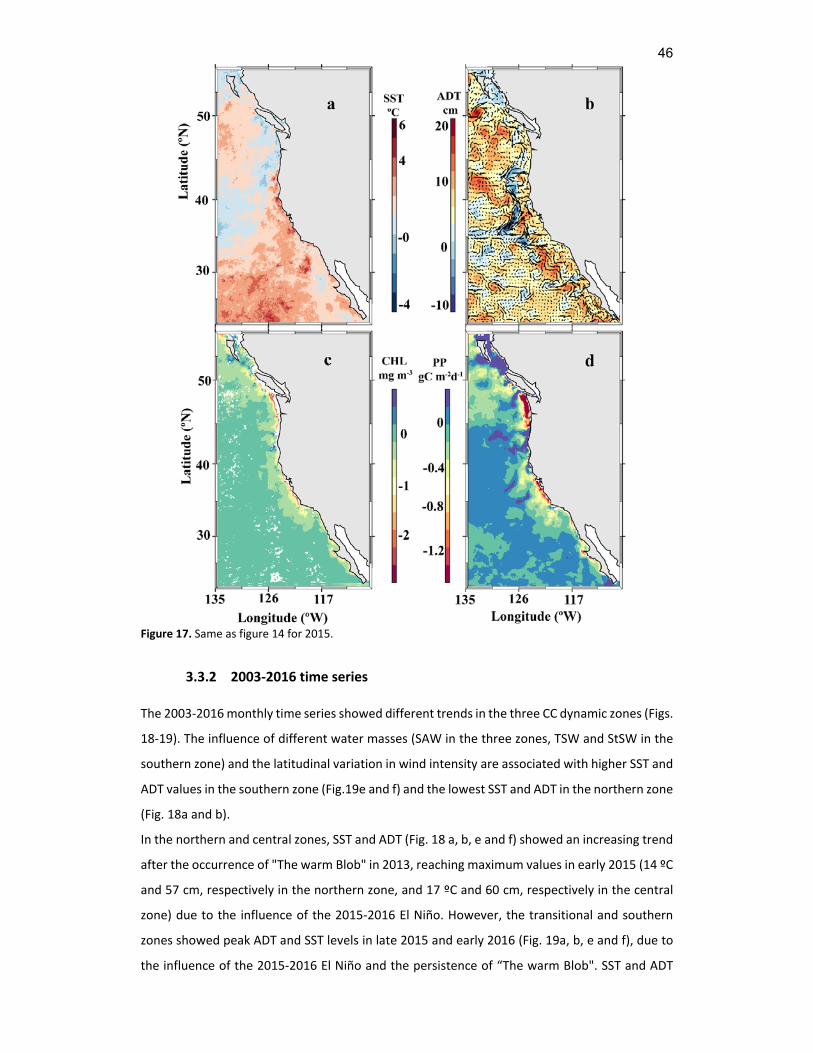
46

Figure 17. Same as figure 14 for 2015.

3.3.2 2003‐2016 time series

The 2003‐2016 monthly time series showed different trends in the three CC dynamic zones (Figs.

18‐19). The influence of different water masses (SAW in the three zones, TSW and StSW in the

southern zone) and the latitudinal variation in wind intensity are associated with higher SST and

ADT values in the southern zone (Fig.19e and f) and the lowest SST and ADT in the northern zone

(Fig. 18a and b).

In the northern and central zones, SST and ADT (Fig. 18 a, b, e and f) showed an increasing trend

after the occurrence of "The warm Blob" in 2013, reaching maximum values in early 2015 (14 ºC

and 57 cm, respectively in the northern zone, and 17 ºC and 60 cm, respectively in the central

zone) due to the influence of the 2015‐2016 El Niño. However, the transitional and southern

zones showed peak ADT and SST levels in late 2015 and early 2016 (Fig. 19a, b, e and f), due to

the influence of the 2015‐2016 El Niño and the persistence of “The warm Blob". SST and ADT

47

values recorded in 2015 in the four areas, were the highest recorded in the last 12 years.

Figure 18. Monthly time series (2003‐2016) in the CC north (left panel) and central zones (rigth panel) for:

sea surface temperature (SST, a, e; °C), absolute dynamic topography (ADT, b, f; cm), satellital chlorophyll

(CHL, c, g; mg m‐3), and primary production (PP, d, h; gC m‐2 d‐1). Black line represents the running average

(12 months) for each data point. Dashed lines indicate the warm Blob in 2013 and 2016 El Niño. The

horizontal dashed line in CHL and PP indicates the trend significant in a pvalue < 0.05. Only the trends with

slope > 0.001 are shown.

In the north and central zones, phytoplankton production and biomass displayed an increasing

trend after the occurrence of the “The warm Blob” (Fig. 18c, d, g and h). However, in early 2015

the annual mean CHL dropped drastically to ~0.3 mgˑm ‐3 in the central zone due to the warming

of the 2015‐2016 El Niño. Unlike the northern and central zones, CHL in the transitional and

southern zones, and PP in the transitional zone, decreased from 2012 onwards (Fig. 19c, d and

g), with the lowest values of the entire series (CHL ~ 0.2 mgˑm‐3 and PP ~ 0.45 gCˑm‐2ˑd‐1 in

transitional zone, and CHL ~ 0.2 mgˑm‐3 and PP ~ 0.3 gCˑm‐2ˑd‐1 in south zone) in the summer of

2016.

48

The 2003‐2016 CHL time series showed a negative trend in most of the CC zones, except for the

Northern zone. The central zone showed the largest decreases, while in the transitional and the

south zones the slope was moderately negative. The decrease in PP was only evident in the

transitional zone. Thus, all the CC zones at latitudes < 35°N showed a decline in phytoplankton

biomass between 2003 and 2016.

Figure 19. Same as Figure 17, for the transitional and south CC zones.

To quantify the changes in the analyzed variables, the long‐term means of the time series were

subtracted from the monthly values as shown in Fig. 20 and 21. The occurrence of "The warm

Blob" became evident by mid‐2013 in the temperature anomalies (SSTa) of the four CC zones,

reaching a maximum of ~ 2 ºC in the first half of 2016 in the northern zone and at the end of

2015 in the other CC zones. "The warm Blob" had opposite effects on phytoplankton biomass

and production in the northern and central zones compared to the transitional and southern

zones. During the warm 2013‐2016 period, increases in phytoplankton biomass and production

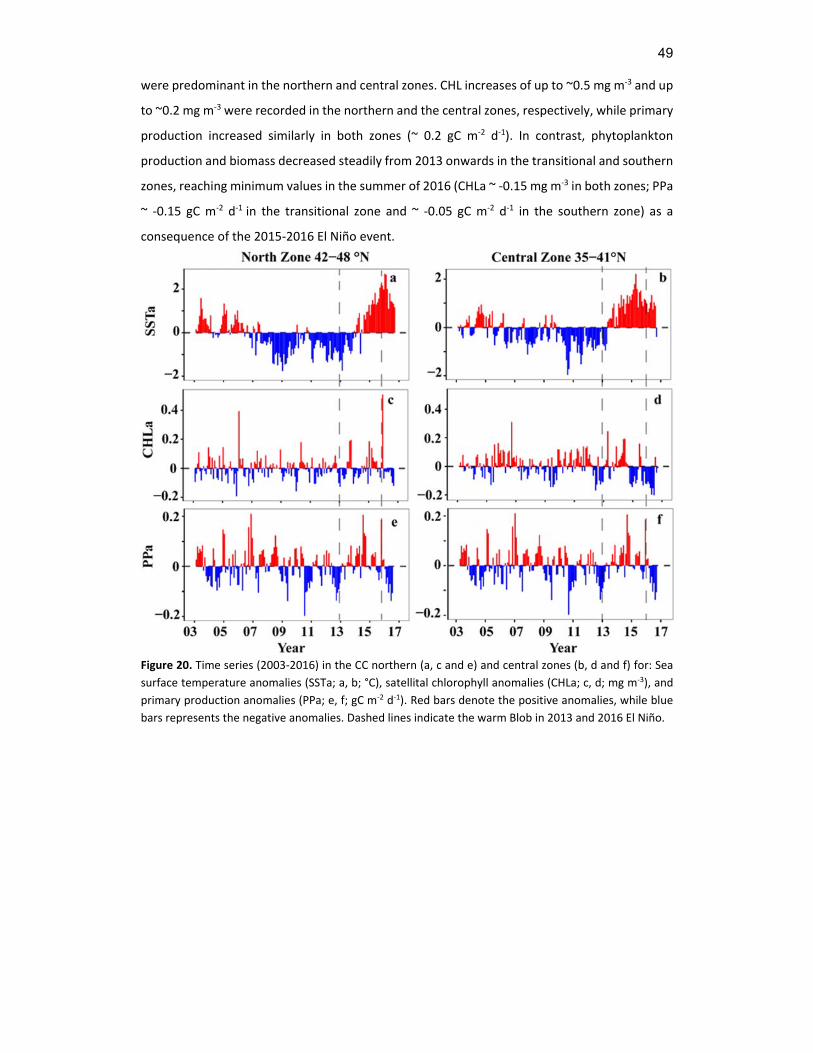
49

were predominant in the northern and central zones. CHL increases of up to ~0.5 mg m‐3 and up

to ~0.2 mg m‐3 were recorded in the northern and the central zones, respectively, while primary

production increased similarly in both zones (~ 0.2 gC m‐2 d‐1). In contrast, phytoplankton

production and biomass decreased steadily from 2013 onwards in the transitional and southern

zones, reaching minimum values in the summer of 2016 (CHLa ~ ‐0.15 mg m‐3 in both zones; PPa

~ ‐0.15 gC m‐2 d‐1 in the transitional zone and ~ ‐0.05 gC m‐2 d‐1 in the southern zone) as a

consequence of the 2015‐2016 El Niño event.

Figure 20. Time series (2003‐2016) in the CC northern (a, c and e) and central zones (b, d and f) for: Sea

surface temperature anomalies (SSTa; a, b; °C), satellital chlorophyll anomalies (CHLa; c, d; mg m‐3), and

primary production anomalies (PPa; e, f; gC m‐2 d‐1). Red bars denote the positive anomalies, while blue

bars represents the negative anomalies. Dashed lines indicate the warm Blob in 2013 and 2016 El Niño.

50

3.4 Discussion

3.4.1 "The Blob" and El Niño

Based on the long‐term summer averages of in‐situ and remote sensing (2003‐2015)

observations, the CCS region can be regarded as an ecosystem with latitudinal variation, from

predominantly temperate conditions in the northern and central zones, to temperate‐to‐

tropical transitional conditions in the southern zone. In the upper water column (0‐100m), the

influence of different water masses [SAW in the three zones, Lynn and Simpson,( 1987); TSW

and StSW in the southern zone, Roden, (1971); Durazo, (2015)] and the latitudinal variation in

wind intensity (Huyer, 1983) are associated with higher SST and ADT and lower CHL values in the

southern zone, while the opposite is true in the northern zone. In the summer average, the CCS

has a high biological production supported by coastal upwelling processes that make it an

ecosystem with favorable conditions for phytoplankton growth that sustains higher trophic

levels.

“The warm Blob” produced anomalously warm conditions in the ocean which, for the first time

in the records, preceded an El Niño event. For the CC central and southern zones, Jacox et al.

(2016) reported that although SST anomalies in the tropical Pacific were very large in late 2015,

those did not occur in conjunction with strong equatorial Kelvin waves and a weakening of the

Figure 21. Same as figure 8 but transitional (a, c, and e) and south zones (b, d, and f).

51

upwelling‐driving winds. On the contrary, their results showed that upwelling‐driving winds

were anomalously strong during the autumn of 2015. Despite this, the pycnocline (isopycnal

surface of 26 kg m‐3 σθ), which had deepened since mid‐2014, remained deep until late 2015 and

early 2016 (Zaba and Rudnick, 2016). However, our results showed that for the four CC zones,

the dynamic height increased from 2013 to early 2016, reaching its maximum during the second

half of 2015. Therefore, the ocean warming caused by “The warm Blob” from 2013 to 2015

caused physical and biological changes in the California Current ecosystem that preceded the

2015‐2016 El Niño which, although atypical, prevented the ecosystem recovery. This was evident

in the 2016 phytoplankton biomass and production values which were the lowest ones recorded

in the last 13 years.

As we noted above, the largest temperature anomalies in the CCS during 2013‐2014 occurred in

the coastal region of the southern zone off Baja California. These temperature values may have

been caused by a surface warming caused by a second patch of the anomalously warm water

brought about by “The warm Blob” off Baja California in the spring of 2014 (Cavole et al., 2016),

which may have promoted the development of a poleward coastal flow advecting relatively

warm and saltier waters, as is reflected in the positive temperature and salinity anomalies of

figure 14. This might have prevented the upward sloping of isopycnals (isotherms) in the coastal

region which usually lead to low coastal sea surface temperatures in the summer (Durazo, 2015).

In contrast, the weakening of the upwelling‐driving northwesterly winds in 2014 (Bond et al.,

2015), along with the density readjustment of the depth of CC water below warmer surface

water (evidenced in the negative salinity anomalies below 50 m depth), caused the sinking of

isopycnals (nutricline) that led to the interruption or inhibition of upwelling events and resulted

in both very high near‐surface temperatures and a decrease in phytoplankton biomass.

On the other hand, it is worth noting that El Niño, although weak in 2014‐2015, may have

provided a feedback mechanism to “The warm Blob" through an atmospheric teleconnection

from the equator to the Baja California peninsula region. This phenomenon has been detected

in other El Niño years (Durazo and Baumgartner, 2002). It has recently been observed that the

atmospheric teleconnection with ENSO during the winter of 2015 was associated with the

persistence of “The warm Blob", accounting for 50% to the variance in sea‐level pressure in the

North Pacific (Di Lorenzo and Mantua, 2015).

Although positive temperature and ADT anomalies were also recorded in the offshore region,

phytoplankton biomass and production displayed average summer values during the summers

of 2014 and 2015 in this zone. This may be explained by the fact that the small‐sized

phytoplankton groups typical of oceanic regions are favored by warm oligotrophic conditions

(Barber and Hiscock, 2006) such as those occurring during "The warm Blob" and El Niño, whereas

the larger primary producers that are common in upwelling areas (e.g.. diatoms) are favored by

52

high nutrient levels and colder waters (Hinz et al., 2012). This may explain the near‐average PP

and CHL values recorded in the oceanic region during the summers of 2014 and 2015 and their

decrease in the coastal region. Therefore, the warm water during the 2014 "The warm Blob" that

persisted in 2016 due to the warm ENSO modified the thermodynamics of the water column,

produced changes in the circulation and adversely affected the pelagic ecosystem in the CC area,

mainly in the coastal region.

3.4.2 Trends and climatic indices

Indices of large‐scale climate variability such as the PDO, NPGO, MEI and ONI (Fig. 22) are often

used to explain physical and biological fluctuations in the Northeast Pacific Ocean (Lynn et al.,

1998; Lavaniegos and Ohman, 2003; Di Lorenzo et al., 2008). Changes in the magnitude and sign

of the indices have been correlated with variations in marine ecosystems. Positive PDO and

negative NPGO values denote the weakening of coastal upwelling and the ensuing reduction of

the mixing and turbulent transport of nutrients to the euphotic zone. Similarly, positive MEI

values denote the deepening of the nutricline in the California Current region caused by the

poleward propagation of the coastal Kelvin wave associated to ENSO events.

Figure 22. Climatic indices: a) Pacific Decadal Oscillation (PDO), b) North Pacific Gyre Oscillation (NPGO),

c) Multivariate ENSO Index (MEI), and d) Oceanic Niño Index (ONI).

53

To better understand the trends observed in the physical (SST and ADT) and biological (CHL and

PP) variables, we compared these time series to the above‐mentioned climatic indices (Fig. 22).

The PDO (Fig. 22a) shows the cold‐to‐warm transition since 2015, while the NPGO (Fig.

22b) displays the transition from a moderately positive phase from 2007 to 2014 to a negative

one in early 2014 when “The warm Blob” became evident in the CC region. The MEI (Fig. 22c)

and ONI (Fig. 22d) indices show the transition from a negative to a positive phase starting in mid‐

2014, and reach their maximum values in early 2016. Therefore, physical processes related to

the oceanic indices as discussed above might explain the trend observed in the CC area toward

an increase in the stratification of the water column and a decline in phytoplankton biomass,

both affecting the epipelagic ecosystem from primary producers to the upper trophic levels.

To explore the relationship between changes in ocean circulation and fluctuations in

phytoplankton biomass in the CC, we calculated correlation coefficients between the PDO,

NPGO, MEI and ONI indices and the CHLa time series. No statistically significant correlation was

found between these indices and CHLa in the north zone (42‐48 °N). In the central zone (35‐41

°N), CHLa was significantly correlated only with PDO and MEI, although such correlations were

moderately low (PDO, r = ‐0.22 and MEI, r = ‐0.3). Significant correlations with NPGO were found

at latitudes <32 °N but were also moderately low (0.3 in the transition zone and 0.24 in the Baja

California area, P = 0.001). Previous studies have shown that the upwelling variability along the

Northeast Pacific coast is strongly correlated with NPGO only south of 38 °N; farther north,

upwelling is more strongly controlled by changes in along shore winds correlated with PDO (Di

Lorenzo et al., 2008). Di Lorenzo et al. (2008) found a strong correlation between NPGO and

variables characteristic of coastal upwelling such as nutrients, salinity, upwelling‐driving winds

and in situ surface chlorophyll, which were not analyzed in this work. In contrast, PDO showed

a high correlation with CHLa in the transitional (‐0.6) and the southern (‐0.5) zones of the CC off

Baja California. The correlation between CHLa and the El Niño‐related indices (MEI and ONI)

increased from north to south (between ‐0.4 and ‐0.5 for the transition and southern zones). It

is expected that subtropical latitudes <32 °N are more affected by ENSO than more northern

areas of the Pacific since, in addition to the Kelvin waves carrying the ENSO equatorial signal

poleward along the coast and to the atmospheric teleconnections, the southern zone of the CC,

particularly at latitudes <28 ° N, is influenced by water masses of tropical origin.

The weakening of the California Current and the strengthening of the Aleutian low pressure

system (weakening of winds along the coast) (positive PDO and negative NPGO) are evident in

the increase in temperature and dynamic height in the California Current’s area of influence, as

they lead to a reduction in the influx of low‐temperature water from two sources: the first one

of Sub‐Arctic origin and transported by the California Current, and the second one originating

from coastal upwellings (Chhak and Di Lorenzo, 2007; Di Lorenzo et al., 2008). The decline in

54

phytoplankton biomass in the northern and central areas of the CC coincided with the phase

change of the PDO in 2015. Additionally, in all the zones the most drastic drop in phytoplankton

biomass and production (except for PPa in the Baja California zone) coincided with the highest

(or most negative) values of the indices analyzed, which occurred during 2016. Thus, the

weakening of the California Current and coastal upwelling during 2013‐2014 (when the NPGO

changed phase), together with the warm water pools generated during "The warm Blob",

provided a warm, stratified habitat for phytoplankton in this area.

The 2013‐2015 phytoplankton production and biomass time series for the north and central

zones of the California Current showed opposite trends to those for the transitional and Baja

California zones. Despite the large positive SST anomalies observed during the 2013‐2015 period

in the Northeastern Pacific, CHL and PP showed an increasing trend in the northern (42‐48°N)

and central (35‐41°N) zones of the California Current. Similarly to the north and central zones,

phytoplankton biomass and production in the Alaskan Gyre increased over the 2013‐2015 period

(results not shown). A similar situation was reported for the late 1970s and 1980s, when

biological variables showed higher fish and zooplankton densities when de Aleutian Low

Pressure System was more intense than the average (Polovina et al., 1995). For Alaskan salmon,

the typical positive PDO year brings enhanced stream‐flows and nearshore ocean mixed‐layer

conditions that are favorable to high biological productivity (Mantua et al., 1997). Although river

nutrients can have a small impact on primary production at the annual time scale and moderate

at the seasonal scale (Tremblay et al., 2014), nutrient inputs from rivers, along with warm

temperatures and a shallow nutricline, create an environment favorable for phytoplankton

growth in spite of warm ocean anomalies. Phytoplankton growth rates benefit from the

increased water temperature (Eppley, 1972) and high nutrient concentrations (Duarte et al.,

2000). In addition, a shallow nutricline allows them to remain in the euphotic zone to carry out

photosynthesis and increase their biomass. The northern zone of the CC limits with the Alaskan

Gyre (48 ° N) and, therefore, the increase in CHL and PP over the 2013‐2015 period might be

related to the influence of processes occurring in the Alaskan Gyre during the same period,

which could hypothetically be similar to those described by Mantua et al. (1997). However,

further studies, beyond the scope of this study, are necessary to test this hypothesis. The

opposite scenario occurred in the transitional and the Baja California zones, where the main

nutrient input and the lifting of the isopycnals are given by coastal upwelling. Therefore, the

upwelling weakening and the warming of the ocean surface layer from 2013 to 2015 led to

thermocline deepening and nutrient impoverishment in the euphotic zone, resulting in a

reduction in phytoplankton biomass and production in the transitional and Baja California zones.

Despite the high positive SST anomalies reported for the 2013‐2014 winter in the Northeastern

Pacific (Bond et al., 2015), SST and ADT showed an increase after the 2010 La Niña event,

55

whereas CHL and PP decreased from 2012 to 2016 in the transitional and Baja California zones.

The CalCOFI program reported a decline in fish and invertebrate stocks (standing stock) starting

in 2011 (Rodriguez et al., 2015). Commercial fisheries in the CalCOFI region reported a 36%

decline in 2014, relative to the peak amount caught in 2000 (Rodriguez et al., 2015). Similarly,

based on the annual fish landings report of the California Department of Fish and Wildlife, the

2015 fish landings show a 23% drop compared to those recorded in 2013 in Baja California

waters. This suggests that changes in the structure of the water column began to appear in 2011

in the southern zone of the CC; such changes affected the phytoplankton biomass and

production and higher trophic levels. However, the underlying reasons for these changes are still

uncertain.

3.4.3 Optimal ADT window for phytoplankton production

Approximate physical dynamic thresholds have been estimated for other organisms. Asch and

Checkley (2013) found that the greatest probability of encountering anchovy, sardine, and jack

mackerel eggs occurs at dynamic heights of 79–83 cm, 84–89 cm, and 89–99 cm, respectively.

Optimum habitats at absolute dynamic topography values of 48.7 to 50.7 cm for blue whales

and 43.7 to 50.7 cm for short‐beaked common dolphins were estimated by Pardo et al. (2015).

Therefore, we also explored whether an ADT threshold exists for phytoplankton primary

production that might explain its decline over the 2011‐2016 period in the California Current

region.

The declining trend in phytoplankton biomass and production matches the increase in the ADT

and SST time series (2003‐2016) for the three zones of the CCS. The inverse relationship between

these trends was analyzed using GAMs. The curve that resulted from modeling the relationship

between ADT and PP over the 1997‐2015 period (Fig. 23) showed two ADT ranges in which PP

decreased: the first between 17 cm and 39 cm, and the second between 64.5 cm and 102 cm.

The optimal window for primary production was observed at ADT values ranging from 39 cm to

64.5 cm.

The ADT ranges that led to a decline in PP are typical of waters that are either highly mixed (low

ADT) or highly stratified (higher ADT) (Rebert et al., 1985; Beier, 1997; Kessler, 2006). The high

56

vertical mixing in the water column has been associated with photo acclimation of

phytoplankton to intermediate irradiance regimes, which modify some photosynthetic

parameters . This is explained by the fact that vertical advection in a highly mixed water column

carries phytoplankton across large irradiance gradients, which prevents its adaptation and

consequently results in very low or nil increase in either biomass or production. The high

photosynthetic capacity of phytoplankton under light at saturation level (a parameter of

phytoplankton photosynthesis known as P ) has been associated with intermediate

stratification levels, while low P are related to both very high and very low stratification

levels (Álvarez‐Borrego and Gaxiola‐Castro, 1988; Gaxiola‐Castro et al., 1999). According

to Behrenfeld and Falkowski (1997), the change in P with sea surface temperature is not linear,

with peak values at intermediate temperatures (15‐20 °C). Additionally, different taxonomic

groups of phytoplankton have different optimal temperatures for growth (Eppley, 1972), and

the phytoplankton growth rate usually decreases as temperature drops. PP reaches peak levels

when growth rates are optimal and the phytoplankton standing stock is maximum. In a highly

stratified water column (higher ADT), the thermocline (nutricline) deepens and phytoplankton

becomes exposed to a lesser irradiance gradient, since it can be carried beyond the euphotic

zone, leading to a decrease in PP due to very low irradiance levels. Furthermore, another limiting

factor in these environments is nutrient availability within the euphotic zone, which translates

into lower phytoplankton PP and biomass. Therefore, the optimum habitat for phytoplankton

includes intermediate ADT values, typical of a moderately mixed water column, and the

thermocline (nutricline) located within the euphotic zone.

Figure 23. Results of the Generalized Additive Model (GAM) functions, illustrating the partial response of

integrated PP to Absolute Dynamic Topography (ADT). The smooth function (solid line) with 95%

confidence interval (shaded area are shown for the predictor variable). Rug lines on the x‐axis represent

the values observed. Labels on the y‐axis show the effective degrees of freedom for the smooth terms of

GAMs. Vertical dashed lines limit the range of ADT values for which positive effects on PP were observed.

57

Previous studies have used variables such as SST to study the effect of stratification on

phytoplankton. In our case, we used ADT as an indicator of changes in the habitat of

phytoplankton influenced by the water column dynamics. Low PP levels will be observed in a

highly dynamic (low ADT) or stratified (high ADT) environment, whereas peak PP levels will occur

at intermediate conditions. Increased sea level may influence phytoplankton due to the

deepening of the photic zone. In a two‐layer ocean, sea‐surface level variability may be a good

indicator of thermocline adjustment (Gill, 1982). Roughly, for a 10 cm sea surface rising, a

thermocline (pycnocline) subsidence of approximately 25 m can be expected (Beier, 1997).

During the summers 2014 and 2015, ADT was between 10 and 20 cm above the average, which

is equivalent to a 25‐50 m sinking of the thermocline. The decline in phytoplankton biomass and

production during the summers of 2014 and 2015, under the effects of "The warm Blob" and the

2014‐2015 El Niño, was probably due to the low nutrient availability and irradiance for

phytoplankton as a result of such deepening.

3.5 Conclusions

The high positive temperature anomalies in the upper portion of the water column that occurred

during the summers of 2014 and 2015 negatively impacted the epipelagic ecosystem of the

California Current by reducing dramatically the amount of biomass (phytoplankton) available for

the upper trophic levels. We noted that as long as the latitudinal gradients are maintained in

terms of the magnitudes of the physical and biological variables in the three zones, the

persistent pattern in the area points was to the rise in both sea surface temperature and sea

level, with a consequent decrease in phytoplankton production and biomass. The warm surface

water produced as a result of "The Blob" and the 2015‐2016 El Niño translated into the

deepening of the water core of the California Current, resulting in the reorganization of the

physicochemical structure of the water column and the decline in biomass and primary

production. Although phytoplankton production and biomass decreased over the past 3‐4 years,

the mechanisms that led to this trend are seemingly related to a climate shift from cold to warm

in the northeastern Pacific Ocean. Assuming that phytoplankton abundance will continue

declining at the global level in response to the warming and stratification of the ocean (Boyce et

al., 2010), the statistical estimates on the thresholds at which the physical stressors (example:

SST and ADT) impact either positively or negatively marine organisms will be a valuable and

suitable tool to facilitate prediction‐making about the likely changes of marine ecosystems.

58

4. Chapter 4: General discussion

The underlying hypothesis outlined above was that the highest productive areas in the ocean

are the result of physical processes associated to ocean circulation, which are detectable as low

ADT and high positive EkP conditions, whereas the opposite occurs in less productive areas.

The thresholds of mixed layer and pycnocline depth, ADT, and EkP established the selected

ranges at which phytoplankton variations occurs at the seasonal, and interannual scales. The

results of this work will be a useful tool for studies where phytoplankton production and biomass

data are not available. Phytoplankton is the first level of the marine food web, so changes in

upper trophic levels might be explained by phytoplankton changes. Moreover, if there were no

in situ temperature and salinity data, ADT and EkP derived from satellite data can be proxies of

the water column structure, and their values will allow to do estimations of water column

productivity through the GAM’s smoothed functions estimated here.

In the next sections, we will focus on analyzing the main results of this work emphasizing the

influence of the physical variables studied here on phytoplankton, as well as on the mechanisms

and the ecological adaptations of phytoplanktonic groups to habitat conditions generated by

physical processes occurring in the ocean surface. First, the effect of mixed layer and pycnocline

changes on phytoplankton will be described, and then ‐based on other studies‐ its variability in

subtropical‐tropical zones and their implications for phytoplankton organisms will also be

described. Second, the ADT thresholds and their link with water column structure and

productivity will be analyzed. Third, the EkP role at the seasonal scale will be considered. Finally,

a general conclusion about the importance of thresholds in ecology will be addressed.

4.1 Shallower mixed layer threshold for PP than for Chla

Physiology of phytoplankton is affected directly by MLD. Irradiance and the average

photosynthetic rate of algal cells decrease with the increasing of the mixed layer thickness. MLD

is deep when there is turbulence at the upper layer, becoming well mixed and enriched of

nutrients. However, when the above occurs, phytoplankton organisms are moved toward

depths with low irradiance, and they could be transported below depths corresponding to the

50% of surface irradiance level. Therefore, when there are low light conditions the rate of

primary production is reduced. Acclimation of photosynthetic parameters of different taxa to

environmental factors including light, nutrients and temperature are not well specified.

However, it is also known that nutrient and temperature regulation can lead to significant

changes in the maximum quantum yield, and the individual response of different taxonomic

groups may differ considerably (Aguirre‐Hernández et al., 2004). Álvarez‐Borrego and Gaxiola‐

Castro (1988) and Gaxiola‐Castro et al. (1999) observed that the maximum phytoplankton

photosynthetic rates decreased in a zone of the Gulf of California with intense mixing. They

59

explained that in summer and autumn SST increased, and thus a stratified water column allowed

phytoplankton cells to remain close to the surface, therefore the organisms acclimated to high

irradiance and the maximum phytoplankton photosynthetic rates increased. Although the

influence of MLD on phytoplankton has been already described in early (Marra, 1978) and recent

studies (Behrenfeld and Boss, 2014), my results provide a tool to infer high productivity when

MLD < 20 m, in studies where phytoplankton production and biomass data are not available.

The Pacific Ocean off Mexico showed maximum phytoplankton biomass in spring‐summer in the

subtropical zone, and in winter‐spring in the tropical zone, when shallow MLD occurred.

Jeronimo and Gomez‐Valdes (2010) observed contours of constant MLD parallel to the coast in

the subtropical zone, with MLD decreasing onshore, with the deepest thickness (~70 m) in

January, and the shallowest (~15 m) in July. They attributed MLD variability mainly to wind

driven phenomena, except during the heating period. Similarly, López‐Sandoval et al. (2009)

observed that coastal upwelling occurs from March through June in the tropical zone, where

they observed the rising of isotherms toward the coast and a mixed surface layer thinning in the

same direction. The linking between MLD and biomass suggests that MLD variability may explain

phytoplankton production and biomass maxima in spring‐summer and minima in autumn‐

winter. This result is consistent with the study made for Raitsos et al. (2012) who found that

surface phytoplankton blooms appeared to be favored by cold, nutrient rich, well mixed and

higher salinity waters. Using GAM analysis they found that at depths larger than 40 m,

chlorophyll ceases to increase. Thus, this supports the idea that MLD thresholds established here

(Fig. 8) may explain integrated PP and Chla seasonal variability, with high values occurring at

MLD < 20 m.

4.2 ADT as a proxy of water column productivity

When the study area was extended to the California Current region, the ADT threshold was

wider (Fig. 21) than that estimated for subtropical‐tropical Pacific Ocean off Mexico (Fig. 7).

However, ADT thresholds between 40 cm and 80 cm had the same relationship in both regions.

GAM’s –derived ADT thresholds over PP showed that levels of ADT between 40 and 60 cm

increase PP, and values outside those thresholds have a negative effect on PP. Results of this

study show that the maximum phytoplankton biomass and production occurred in the upwelling

season (spring‐ early summer) where ADT is the lowest for the entire year. Low ADT is related

with the turbulent transport of nutrients towards the euphotic zone, which in turn are used by

phytoplankton for growth. Therefore, when nutrient data are not available, ADT may be a very

good proxy for nutrient turbulent transport, with the optimal ADT window for PP at 40‐60 cm.

Stratification in our study area is clearly defined in summer and autumn (Gaxiola‐Castro and

Durazo, 2010). This is originated by weakening of winds and the increase in heat gain by the

60

ocean (during summer through winter), benefiting vertical stratification. The duration of

stratification is critical for increasing or decreasing PP (Tilstone et al., 1999). Long periods of

stratification tend to result in low PP due to nutrient consumption and limitation, and due to the

sinking of phytoplankton from the euphotic zone. The alternation between well mixed water

column due to stronger winds, and stratification due to water column heating, have been

reported to yield high PP as long as light and nutrients are not limiting (Brown and Field,1986;

Legendre,1981). Results of the present study clearly show the link between high ADT and water

column productivity. Consequently, ADT may be a good proxy for water column phytoplankton

productivity.

4.3 Ekman pumping as the dominant forcing of phytoplankton

seasonal variability

Ekman pumping occur when wind stress leads to a divergence of Ekman transport and deeper

water rises to take its place. Ekman pumping is one of the mechanisms of the dominant forcing

of near‐surface circulation driven by wind stress. Gaxiola‐Castro and Durazo (2010) described

that off the Baja California peninsula, wind stress curl is cyclonic on well‐defined areas near the

coast, with greater intensity in spring and summer, and decays offshore changing to anticyclonic.

At the entrance to the Gulf of California, wind stress curl is positive except during winter. A

persistent positive wind stress curl promotes cyclonic circulation facilitating upward pycnocline

movements. High Ekman pumping and phytoplankton biomass in the coastal region of the

tropical and subtropical zones were observed, during spring‐summer, when alongshore winds

are strong. Accordingly, coastal upwelling and Ekman pumping are the main mechanisms driving

the seasonal phytoplankton variability in tropical‐subtropical zones of the Pacific Ocean off

Mexico.

4.4 Physical processes as drivers of phytoplankton habitat conditions

Phytoplanktonic groups are directly related to physical habitat conditions. Typically, the cold and

nutrient‐rich upwelling areas are dominated by larger phytoplanktonic organisms like diatoms

(20‐200 µm) (Hinz et al., 2012), while in warm and oligotrophic environments like oceanic zones,

smaller phytoplanktonic organisms are more abundant (pico‐plankton, between 0.2 µm and 2

µm, and nano‐plankton from 2 µm to 20 µm) (Barber and Hiscock, 2006).Thus, during

oligotrophic (high nutrient) conditions, as in autumn‐winter (spring‐summer), and El Niño (La

Niña), , the successional replacement of smaller (larger) phytoplanktonic cells by larger (smaller)

phytoplanktonic cells in response of cooling (warming) conditions is observed mainly in the

coastal zone. On the other hand, the smaller phytoplankton ubiquitous in the oceanic zones is

favored during the warm and oligotrophic El Niño conditions, while the larger primary producers

61

are favored by the cool and high nutrient La Niña conditions. Moreover, the oceanic region is

favored during La Niña, due to the rich nutrient upwelled waters carried offshore by the strong

Ekman transport, fertilizing the offshore euphotic layer, increasing both primary production and

phytoplankton biomass, and moving drifting microorganisms long distances away from the their

natural habitat (Linacre et al., 2010). For example, in the tropical zone, Franco‐Gordo et al.

(2004) observed changes in the phytoplankton community structure pattern from high

abundances inshore to low offshore, to uniform abundances offshore‐inshore during El Niño

conditions. In contrast, during La Niña 2008, the phytoplankton biomass and production

estimates of smaller phytoplankton were at their lowest levels off Baja California, suggesting

that the smallest primary producers were being replaced by larger cells (Linacre et al., 2010).

Following other studies and the results of these work, they may suggest that the near‐surface

circulation features such as temperature, nutrient source, and turbulence, establish

environmental factors limiting phytoplankton growth. Different types of habitats generated by

physical processes favor the development of specific phytoplankton groups with physiological

footprints given by evolutionary processes, which will determine phytoplankton production and

biomass regional patterns.

4.5 Concluding remarks

The identification of ecological thresholds in marine ecosystems may be useful for scientists as

it can help to understand ecosystems variability at mesoscale, seasonal, and interannual scales.

Despite the effects of physical processes on phytoplankton has been broadly discussed, there

are few studies where the thresholds of variables related to physical processes are estimated.

In this study, advanced statistical methods helped to estimate complex relationships between

ecosystem environmental drivers and organisms. The importance of physical processes as

drivers of phytoplankton habitat, and its implications, is confirmed. Moreover, a valuable tool

for scientists, to better understand the physics‐biological interactions between phytoplankton

and its environment, is presented. However, in order to improve and complete the results

obtained here, more in situ sampling efforts, and the continuity of monitoring programs of

marine ecosystems are necessary, such as CalCOFI and IMECOCAL.

62

5. Cited Literature

Aguirre‐Hernández, E., Gaxiola‐Castro, G., Nájera‐Martínez, S., Baumgartner, T., Kahru, M., and Greg Mitchell, B. 2004. Phytoplankton absorption, photosynthetic parameters, and primary production off Baja California: Summer and autumn 1998. Deep‐Sea Research Part II: Topical Studies in Oceanography, 51: 799–816.

Álvarez‐Borrego, S., and Gaxiola‐Castro, G. 1988. Photosynthetic parameters of Northern Gulf of California phytoplankton. Continental Shelf Research, 8: 37–47.

Asch, R. G., and Checkley, D. M. 2013. Dynamic height: A key variable for identifying the spawning habitat of small pelagic fishes. Deep‐Sea Research Part I: Oceanographic Research Papers, 71: 79–91. doi:10.1016/j.dsr.2012.08.006.

Backhaus, J., Hegseth, E., Wehde, H., Irigoien, X., Hatten, K., and Logemann, K. 2003. Convection and primary production in winter. Marine Ecology Progress Series, 251: 1–14.

Banse, K. 1982. Cell volumes, maximal growth rates of unicellular algae and ciliates, and the role of ciliates in the marine pelagial. Limnology & Oceanography, 27: 1059–71.

Barber, R. T., and Hiscock, M. R. 2006. A rising tide lifts all phytoplankton: Growth response of other phytoplankton taxa in diatom‐dominated blooms. Global Biogeochemical Cycles, 20: 1–12.

Behrenfeld, M. J., and Falkowski, P. G. 1997a. Photosynthetic rates derived from satellite‐based chlorophyll concentration. Limnology and Oceanography, 42: 1–20.

Behrenfeld, M. J., and Falkowski, P. G. 1997b. Photosynthetic rates derived from satellite‐based chlorophyll concentration. Limnology and Oceanography, 42: 1–20.

Behrenfeld, M. J., O’Malley, R. T., Siegel, D. a, McClain, C. R., Sarmiento, J. L., Feldman, G. C., Milligan, A. J., et al. 2006. Climate‐driven trends in contemporary ocean productivity. Nature, 444: 752–755.

Behrenfeld, M. J. 2010. Abandoning Sverdrup’s Critical Depth Hypothesis on phytoplankton blooms. Ecology, 91: 977–989. doi: 10.1890/09‐1207.1.

Behrenfeld, M. J., and Boss, E. S. 2014. Resurrecting the Ecological Underpinnings of Ocean Plankton Blooms. Annual Review of Marine Science, 6: 167–194.

Beier, E. 1997. A Numerical Investigation of the Annual Variability in the Gulf of California. Journal of Physical Oceanography, 27: 615–632.

Beisner, B. E., Haydon, D. T., and Cuddington, K. 2003. Alternative stable states in ecology. Frontiers in Ecology and the Environment, 1: 376–382.

Bond, N. A., Cronin, M. F., Freeland, H., and Mantua, N. 2015. Causes and impacts of the 2014 warm anomaly in the NE Pacific. Geophysical Research Letters, 42: 3414–3420. doi: 10.1002/2015GL063306.

Boyce, D. G., Lewis, M. R., and Worm, B. 2010. Global phytoplankton decline over the past century. Nature, 466: 591–596. Nature Publishing Group. doi: 10.1038/nature09268.

Castro, R., and Martinez, J. 2010. Spatial‐temporal variability wind field. In: G. Gaxiola‐Castro and R. Durazo (Ed).Pelagic Ecosystem dynamic off Baja California 1997‐2007 (in spanish), pp. 129–147.

Cavole, L. M., Demko, A. M., Diner, R. E., Giddings, A., Koester, I., Pagniello, C. M. L. ., Paulsen, M. L., et al. 2016. Biological Impacts of the 2013–2015 Warm‐Water Anomaly in the Northeast Pacific. Oceanography, 29: 14.

Cepeda‐Morales, J., Gaxiola‐Castro, G., Beier, E., and Godínez, V. M. 2013. The mechanisms involved in defining the northern boundary of the shallow oxygen minimum zone in the

63

eastern tropical Pacific Ocean off Mexico. Deep Sea Research Part I: Oceanographic Research Papers, 76: 1–12.

Chavez, F. P., Collins, C. A., Huyer, A., and Mackas, D. 2002. El Niño along the west coast of North America. Progress in Oceanography, 54: 1–4.

Checkley, D. M., and Barth, J. A. 2009. Patterns and processes in the California Current System. Progress in Oceanography, 83: 49–64. doi: 10.1016/j.pocean.2009.07.028.

Chelton, D. B., Gaube, P., Schlax, M. G., Early, J. J., and Samelson, R. M. 2011. The Influence of Nonlinear Mesoscale Eddies on Near‐Surface Oceanic Chlorophyll. Science, 334: 328–332.

CoreTeam, R. 2016. A language and environment for Statistical Computing.

Daly, K. L., and Smith, W. O. 1993. Physical‐Biological Interactions Influencing Marine Plankton Production. Annual Review of Ecology and Systematics, 24: 555–585. doi: 10.1146/annurev.es.24.110193.003011.

Di Lorenzo, E., Schneider, N., Cobb, K. M., Franks, P. J. S., Chhak, K., Miller, A. J., Mcwilliams, J. C., et al. 2008. North Pacific Gyre Oscillation links ocean climate and ecosystem change. Geophysical Research Letters, 35: 1–6.

Di Lorenzo, E., and Mantua, N. 2015. Warm Blob in 2014/2015. In Annual meeting PICES 2015. PICES, Quingdao, China, October 19‐27 .

Duarte, C. M., Agustí, S., and Agawin, N. S. R. 2000. Response of a Mediterranean phytoplankton community to increased nutrient inputs: A mesocosm experiment. Marine Ecology Progress Series, 195: 61–70.

Durazo, R., and Baumgartner, T. . 2002. Evolution of oceanographic conditions off Baja California: 1997–1999. Progress in Oceanography, 54: 7–31.

Durazo, R., Gaxiola‐Castro, G., Lavaniegos, B., Castro‐Valdez, R., Gómez‐Valdés, J., and Mascarenhas Jr., A. D. S. 2005b. Oceanographic conditions west of the Baja California coast , 2002 – 2003 : A weak El Niño and subarctic water enhancement. Ciencias Marinas, 31: 537–552.

Durazo, R. 2009. Climate and upper ocean variability off Baja California, Mexico: 1997‐2008. Progress in Oceanography, 83: 361–368. doi: 10.1016/j.pocean.2009.07.043.

Durazo, R. 2015. Seasonality of the transitional region of the California Current System off Baja California. Journal of Geophysical Research: Oceans, 120: 1173–1196.

Eisner, L. B., Gann, J. C., Ladd, C., D. Cieciel, K., and Mordy, C. W. 2015. Late summer/early fall phytoplankton biomass (chlorophyll a) in the eastern Bering Sea: Spatial and temporal variations and factors affecting chlorophyll a concentrations. Deep Sea Research Part II: Topical Studies in Oceanography.

Eppley, R. W. 1972. Temperature and phytoplankton growth in the sea. Fishery Bulletin, 70: 1063–1085.

Espinosa‐Carreon, T. L., Gaxiola‐Castro, G., Beier, E., Strub, P. T., and Kurczyn, J. A. 2012. Effects of mesoscale processes on phytoplankton chlorophyll off Baja California. Journal of Geophysical Research: Oceans, 117: 1–12.

Espinosa‐Carreón, T. L., Gaxiola‐Castro, G., Durazo, R., De la Cruz‐Orozco, M. E., Norzagaray‐Campos, M., and Solana‐Arellano, E. 2015. Influence of anomalous subarctic water intrusion on phytoplankton production off Baja California. Continental Shelf Research, 92: 108–121.

Falkowski, P. G., Ziemann, D., Kolber, Z., and Bienfang, P. K. 1991. Role of Ekman pumping in enhancing primary production in the ocean. Nature, 352: 55–58.

64

Falkowski, P. G., and Oliver, M. J. 2007. Mix and match: how climate selects phytoplankton. Nature Reviews Microbiology, 5: 966–966. doi: 10.1038/nrmicro1792.

Fiedler, P. C., Mendelssohn, R., Palacios, D. M., and Bograd, S. J. 2013. Pycnocline Variations in the Eastern Tropical and North Pacific, 1958–2008. Journal of Climate, 26: 583–599. doi: 10.1175/JCLI‐D‐11‐00728.1.

Franco‐Gordo, C., Godínez‐Domínguez, E., Filonov, A. E., Tereshchenko, I. E., and Freire, J. 2004. Plankton biomass and larval fish abundance prior to and during the El Niño period of 1997‐1998 along the central Pacific coast of México. Progress in Oceanography, 63: 99–123.

Gardner, W. D., Chung, S. P., Richardson, M. J., and Walsh, I. D. 1995. The oceanic mixed‐layer pump. Deep‐Sea Research Part II, 42 (2‐3): 757‐765, 767‐775.

Gardner, W. D., Gundersen, J. S., Richardson, M. J., and Walsh, I. D. 1999. The role of seasonal and diel changes in mixed‐layer depth on carbon and chlorophyll distributions in the Arabian Sea. Deep‐Sea Research Part II: Topical Studies in Oceanography, 46: 1833–1858.

Gaube, P., Chelton, D. B., Strutton, P. G., and Behrenfeld, M. J. 2013. Satellite observations of chlorophyll, phytoplankton biomass, and Ekman pumping in nonlinear mesoscale eddies. Journal of Geophysical Research: Oceans, 118: 6349–6370.

Gaxiola‐Castro, G., Álvarez‐Borrego, S., Lavín, M. F., Zirino, a., and Nájera‐Martínez, S. 1999. Spatial variability of the photosynthetic parameters and biomass of the Gulf of California phytoplankton. Journal of Plankton Research, 21: 231–245.

Gaxiola‐Castro, G., Durazo, R., Lavaniegos, B., De La Cruz‐Orozco, M. E., Millán‐Núñez, E., Soto‐Mardones, L., and Cepeda‐Morales, J. 2008. Pelagic ecosystem response to interannual variability off Baja California. Ciencias Marinas, 34: 263–270.

Gaxiola‐Castro, G. 2010. Pelagic Ecosystem Response to Climate Variability in the Pacific Ocean off Baja California. In Climate Change and Variability, pp. 163–182. Ed. by S. W. Simard and M. E. Austin. Sciyo.

Gill, A. E. 1982. Atmosphere‐ocean dynamics. Academic press, San Diego, California, USA. 645 pp.

Godínez, V. M., Beier, E., Lavín, M. F., and Kurczyn, J. A. 2010. Circulation at the entrance of the Gulf of California from satellite altimeter and hydrographic observations. Journal of Geophysical Research: Oceans, 115: 1–15.

Groffman, P. M., Baron, J. S., Blett, T., Gold, A. J., Goodman, I., Gunderson, L. H., Levinson, B. M., et al. 2006. Ecological Thresholds: The Key to Successful Environmental Management or an Important Concept with No Practical Application? Ecosystems, 9: 1–13. doi:10.1007/s10021‐003‐0142‐z.

Hastie, T. J., and Tibshirani, R. 1986. Generalized additive models,. 3: 297‐‐310. doi:10.1214/ss/1177013604

Hayward, L. T., Baumgartner, T. R., Checkley, D. M., Durazo, R., Gaxiola‐Castro, G., Hyrenbach, K. D., Mantyla, A. W., et al. 1999. The state of the California Current in 1998–1999: Transition to cool‐water conditions. 40: 29–62.

Henson, S. A., and Thomas, A. C. 2007. Phytoplankton scales of variability in the California Current System: 1. Interannual and cross‐shelf variability. Journal of Geophysical Research: Oceans, 112: 1–12.

Hinz, D. J., Nielsdóttir, M. C., Korb, R. E., Whitehouse, M. J., Poulton, A. J., Moore, C. M., Achterberg, E. P., et al. 2012. Responses of microplankton community structure to iron addition in the Scotia Sea. Deep‐Sea Research Part II: Topical Studies in Oceanography, 59–60: 36–46.

65

Holling, C. S. 1973. Resilience and Stability of Ecological Systems. Annual Review of Ecology and Systematics, 4: 1–23. doi:10.1146/annurev.es.04.110173.000245.

Holm‐Hansen, O., Lorenzen, C. J., Holmes, R. W., and Strickland, J. D. H. 1965. Fluorometric Determination of Chlorophyll. ICES Journal of Marine Science, 30: 3–15. doi:10.1093/icesjms/30.1.3

Huyer, A. 1983. Coastal Upwelling in the California current system. Progress in Oceanography, 12: 259–284.

Huyer, A., and Smith, R. L. 1985. The signature of El Niño off Oregon, 1982–1983. Journal of Geophysical Research, 90: 7133.

Jeronimo, G., and Gomez‐Valdes, J. 2010. Mixed layer depth variability in the tropical boundary of the California Current, 1997‐2007. Journal of Geophysical Research: Oceans, 115.

Kahru, M., Kudela, R., Manzano‐Sarabia, M., and Mitchell, B. G. 2009. Trends in primary production in the California Current detected with satellite data. Journal of Geophysical Research: Oceans, 114: 1–7.

Kara, A. ., Rochford, P. A., and Hurlburt, H. E. 2000. An optimal definition for ocean mixed layer depth. Journal of Geophysical Research, 105: 16803–16821. doi: 10.1029/2000JC900072.

Kessler, W. S. 2006. The circulation of the eastern tropical Pacific: A review. Progress in Oceanography, 69: 181–217.

Klein, P., Hua, B.‐L., Le Gentil, S., and Sasaki, H. 2005. The Vertical Pump Organized by the Mesoscale Oceanic Eddies. Annual Report of the Earth Simulator Center: 331–334.

Klein, P., and Lapeyre, G. 2009. The oceanic vertical pump induced by mesoscale and submesoscale turbulence. Annual review of marine science, 1: 351–375.

Kurczyn, J. A., Beier, E., Lavín, M. F., and Chaigneau, A. 2012. Mesoscale eddies in the northeastern Pacific tropical‐subtropical transition zone: Statistical characterization from satellite altimetry. Journal of Geophysical Research: Oceans, 117: 1–17. doi: 10.1029/2012JC007970.

Kurczyn, J. A., Beier, E., Lavín, M. F., Chaigneau, A., and Godínez, V. M. 2013. Anatomy and evolution of a cyclonic mesoscale eddy observed in the northeastern Pacific tropical‐subtropical transition zone. Journal of Geophysical Research: Oceans, 118: 5931–5950. doi: 10.1002/2013JC20437.

Lamont, T., Barlow, R. G., and Kyewalyanga, M. S. 2014. Physical drivers of phytoplankton production in the southern Benguela upwelling system. Deep Sea Research Part I: Oceanographic Research Papers, 90: 1–16.

Lara‐Lara, J. R., and Bazán‐Guzmán, C. 2005. Distribution of chlorophyll and primary production by size classes along the Mexican Pacific coast. Ciencias Marinas, 31: 11–21.

Lavaniegos, B. E., Jiménez‐Pérez, L. C., and Gaxiola‐Castro, G. 2002. Plankton response to El Niño 1997 – 1998 and La Niña 1999 in the southern region of the California Current. Progress in Oceanography, 54: 33–58.

Lavaniegos, B. E., and Ohman, M. D. 2003. Long‐term changes in pelagic tunicates of the California Current. Deep‐Sea Research Part II: Topical Studies in Oceanography, 50: 2473–2498.

Lavín, M. F., Fiedler, P. C., Amador, J. A., Ballance, L. T., Färber‐Lorda, J., and Mestas‐Nuñez, A. M. 2006. A review of eastern tropical Pacific oceanography: Summary. Progress in Oceanography, 69: 391–398.

Leising, A. W., Schroeder, I. D., Bograd, S. J., Abell, J., Durazo, R., Gaxiola‐Castro, G., Bjorkstedt, E., et al. 2015. State of California Current 2014‐15: Impacts of the warm‐water ‘Blob’.

66

CalCOFI Report, 56.

Lin, M., Lucas, H. C., and Galit, S. 2013. Too Big to Fail : Large Samples and the p ‐Value Problem. Information Systems Research: 906–917.

Linacre, L. P., Landry, M. R., Lara‐Lara, J. R., Hernández‐Ayón, J. M., and Bazán‐Guzmán, C. 2010. Picoplankton dynamics during contrasting seasonal oceanographic conditions at a coastal upwelling station off Northern Baja California, México. Journal of Plankton Research, 32: 539–557.

López‐Sandoval, D. C., Lara‐Lara, J. R., Lavín, M. F., Álvarez‐Borrego, S., and G, G.‐C. 2009. Primary productivity in the eastern tropical Pacific off Cabo Corrientes , Mexico. Ciencias Marinas, 35: 169–182.

Lynn, R. J., and Simpson, J. J. 1987. The California Current System: The seasonal variability of its physical characteristics. Journal of Geophysical Research: Oceans (1978–2012), 92: 12947–12966.

Lynn, R. J., Collins, C. a., Mantyla, A. W., Schwing, F. B., Baumgartner, T., Hayward, T. L., Murphree, T., et al. 1998. The state of the California current, 1997‐1998: Transition to El Niño conditions. California Cooperative Oceanic Fisheries Investigations Reports, 39: 25–49.

Mantua, N. J., Hare, S. R., Zhang, Y., Wallace, J. M., and Francis, R. C. 1997. A Pacific Interdecadal Climate Oscillation with Impacts on Salmon Production. Bulletin of the American Meteorological Society, 78: 1069–1079.

Marañón, E., Cermeño, P., Latasa, M., and Tadonléké, R. D. 2012. Temperature, resources, and phytoplankton size structure in the ocean. Limnology and Oceanography, 57: 1266–1278.

Marra, J. 1978. Phytoplankton photosynthetic response to vertical movement in a mixed layer. Marine Biology, 46: 203–208.

McClatchie, S., Goericke, R., Schwing, F. B., Bograd, S. J., Peterson, W. T., Emmett, R., Charter, R., et al. 2009. The state of the California Current, spring 2008‐2009: Cold conditions drive regional differences in coastal production. California Cooperative Oceanic Fisheries Investigations Reports, 50: 43–68.

McGillicuddy, D. J., and Robinson, A. R. 1997. Eddy‐induced nutrient supply and new production in the Sargasso Sea. Deep Sea Research Part I: Oceanographic Research Papers, 44: 1427–1450.

McGillicuddy, D. J., Anderson, L. A., Bates, N. R., Bibby, T., Buesseler, K. O., Carlson, C. A., Davis, C. S., et al. 2007. Eddy/Wind Interactions Stimulate Extraordinary Mid‐Ocean Plankton Blooms. Science, 316: 1021–1026. doi: 10.1126/science.1136256.

McGillicuddy, D. J. 2016. Mechanisms of Physical‐Biological‐Biogeochemical Interaction at the Oceanic Mesoscale. Annual Review of Marine Science, 8: 125–159. doi:10.1146/annurev‐marine‐010814‐015606.

Muradian, R. 2001. Ecological thresholds : a survey. Ecological Economics, 38: 7–24.

Pardo, M. A., Gerrodette, T., Beier, E., Gendron, D., Forney, K. A., Chivers, S. J., Barlow, J., et al. 2015. Inferring Cetacean Population Densities from the Absolute Dynamic Topography of the Ocean in a Hierarchical Bayesian Framework. PLOS ONE, 10: 1–23. doi: 10.1371/journal.pone.0120727

Pares‐Sierra, A., White, W. B., and Tai, C.‐K. 1993. Wind‐driven coastal generation of annual mesoscale eddy activity in the California Current.

Pedlosky, J. 1987. Geophysical Fluid Dynamics. Springer. 705 pp.

Perez‐Brunius, P., Lopez, M., Pares‐Sierra, A., and Pineda, J. 2007. Comparison of upwelling

67

indices off Baja California derived from three different wind data sources. California Cooperative Oceanic Fisheries Investigations Reports, 48: 204–214.

Polovina, J. J., Mitchum, G. T., and Evans, G. T. 1995. Decadal and basin‐scale variation in mixed layer depth and the impact on biological production in the Central and North Pacific, 1960‐88. Deep‐Sea Research Part I, 42: 1701–1716.

Portela, E., Beier, E., Barton, E. D., Castro, R., Godínez, V., Palacios‐Hernández, E., Fiedler, P. C., et al. 2016. Water masses and circulation in the tropical Pacific off central Mexico and surrounding areas. Journal of Physical Oceanography, 46: 3069‐3080. doi: 10.1175/JPO‐D‐16‐0068.1.

Raitsos, D. E., Korres, G., Triantafyllou, G., Petihakis, G., Pantazi, M., Tsiaras, K., and Pollani, A. 2012. Assessing chlorophyll variability in relation to the environmental regime in Pagasitikos Gulf, Greece. Journal of Marine Systems, 94: S16–S22. doi: 10.1016/j.jmarsys.2011.11.003.

Rebert, J. P., Donguy, J. R., Eldin, G., and Wyrtki, K. 1985. Relations between sea level, thermocline depth, heat content, and dynamic height in the tropical Pacific Ocean. Journal of Geophysical Research, 90: 11719.

Roden, G. 1972. Thermohaline structure and baroclinic flow across the Gulf of California entrance and in the Revillagigedo Islands region. Journal of Physical Oceanography, 2: 177–183.

Roden, G. I. 1971. Aspects of the transition zone in the Northeastern Pacific. Journal of Geophysical Research, 76: 3462–3475.

Rodriguez, N., Ryley, L., Budrick, J., Bartling, R., Juhasz, C., Miller, B., Oda, K., et al. 2015. Review of selected California fisheries for 2014 : Coastal pelagic finfish , market squid , gorundfish , Pacific Herring , dungenness crab, ocean Salmon , true smelts , hagfish , and deep water rov surveys of MPAs and surrounding nearshore habitat. California Cooperative Oceanic Fisheries Investigations Report, 56: 1–30.

Schwing, F. B., Moore, C. S., Ralston, S., and Sakuma, K. M. 2000. Record coastal upwelling in the California current in 1999. California Cooperative Oceanic Fisheries Investigations Reports, 41: 148–160.

Schwing, F. B., Bond, N. A., Bograd, S. J., Mitchell, T., Alexander, M. A., and Mantua, N. 2006. Delayed coastal upwelling along the U.S. West Coast in 2005: A historical perspective. Geophysical Research Letters, 33: 1–5.

Siegel, D. A., McGillicuddy, D. J., and Fields, E. A. 1999. Mesoscale eddies, satellite altimetry, and new production in the Sargasso Sea. Journal of Geophysical Research, 104: 13359–13379.

Soto‐Mardones, L., Parés‐Sierra, A., Garcia, J., Durazo, R., and Hormazabal, S. 2004. Analysis of the mesoscale structure in the IMECOCAL region (off Baja California) from hydrographic, ADCP and altimetry data. Deep‐Sea Research Part II: Topical Studies in Oceanography, 51: 785–798.

Steeman Nielsen, E. S. 1952. The use of radio‐active carbon (14C) for measuring organic production in the sea. J. Cons. Explor, 18: 117–140.

Sunda, W. G., and Huntsman, S. A. 1997. Interrelated influence of iron, light and cell size on marine phytoplankton growth. Nature, 390: 389–392. doi: 10.1038/37093.

Tilstone, G., Figueiras, F., Fermín, E., and Arbones, B. 1999. Significance of nanophytoplankton photosynthesis and primary production in a coastal upwelling system (Ría de Vigo, NW Spain). Marine Ecology Progress Series, 183: 13–27.

Tremblay, J., Raimbault, P., Garcia, N., Lansard, B., Babin, M., and Gagnon, J. 2014. Impact of river discharge , upwelling and vertical mixing on the nutrient loading and productivity of

68

the Canadian Beaufort Shelf. Biogeosciences, 11: 4853–4868.

Trenberth, K. E., Large, W. G., and Olson, J. G. 1990. The Mean Annual Cycle in Global Ocean Wind Stress. Journal of Physical Oceanography, 20: 1742–1760.

Venrick, E. L., and Hayward, T. L. 1984. Determining Chlorophyll on the 1984 CALCOFI surveys. CalCOFI Report, 25: 74–79.

Ward, B., and Waniek, J. 2007. Phytoplankton growth conditions during autumn and winter in the Irminger Sea, North Atlantic. Marine Ecology Progress Series, 334: 47–61.

Wood, A. S., Wood, M. S., and Wood, S. 2015. Package ‘ mgcv ’.

Wood, S. N. 2006. Generalized Additive Models: an introduction with R. Chapman & Hall/CRC, Boca Raton, FL. 391 pp.

Xie, Y., Tilstone, G., Widdicombe, C., Woodward, E., Harris, C., and Barnes, M. 2015. Effect of increases in temperature and nutrients on phytoplankton community structure and photosynthesis in the western English Channel. Marine Ecology Progress Series, 519: 61–73.

Yentsch, C. S., and Menzel, D. W. 1963. A method for the determination of phytoplankton chlorophyll and phaeophytin by fluorescence. Deep Sea Research and Oceanographic Abstracts, 10: 221–231.

Yunev, O., Moncheva, S., and Carstensen, J. 2005. Long‐term variability of vertical chlorophyll a and nitrate profiles in the open Black Sea: eutrophication and climate change. Marine Ecology Progress Series, 294: 95–107.

Zaitsev, O., Trasviña‐Castro, A., Linero‐Cueto, J., Gaxiola‐Castro, G., and Cepeda‐Morales, J. 2014. Oceanographic conditions over the continental shelf off Magdalena Bay (Mexico) in 2011–2012. Ciencias Marinas, 40: 89–112.

69

Annexed

Abstract

Generalized additive models (GAMs) were used to estimate the thresholds and contribution of

key dynamic physical variables in terms of phytoplankton production and biomass variability in

the tropical‐subtropical Pacific Ocean off Mexico. The statistical approach used here showed

that the pycnocline and mixed layer depth thresholds were related to high productivity,

thresholds which were shallower for primary production than for phytoplankton biomass

(pycnocline < 68 m and mixed layer < 30 m vs. pycnocline < 45 m and mixed layer < 80 m), but

were similar for absolute dynamic topography and Ekman pumping (ADT<59 cm and EkP > 0 cm

d‐1 vs. ADT < 60 cm and EkP > 4 cm d‐1). The thresholds explained the high productivity on

seasonal (spring) and interannual (La Niña 2008) scales, and were linked to the generally lower

ADT conditions (45‐60 cm), pycnocline depth (9‐68 m), and shallow mixed layer (8‐40 m). Ekman

pumping was mainly related to the seasonal variability associated with alongshore wind during

winter‐spring. In contrast, the biomass depletion recorded in autumn‐winter and during El Niño

conditions was the result of the deepening of the pycnocline and mixed layer as evidenced in

high ADT values. Statistical estimations indicated that the contribution of ocean circulation to

phytoplankton variability was 18% (for phytoplankton biomass), and 46% (for phytoplankton

production), for relationships fitted using satellite data only. This study shows that estimated

thresholds reliably explain the spatial‐temporal variability of phytoplankton in the tropical‐

subtropical Pacific Ocean off the coast of Mexico.

Documents

Programa de Posgrado en Ciencias en Ecología Marina · 2017-02-20 · ii Resumen de tesis presentado por Eliana Gómez Ocampo como requisito parcial para obtener el grado de Doctor