Program • 28.4.

– Model stability analysis – Unexpected model and system behaviour – Modelling structured populations – Example Model in Integrated pest control

• 5.5. no course • 12.5. additional course (O. Jakoby)

– Example bark beetle model – Spatial ecological models

• 19.5. – Forest models, climate change – Large scale spatio-temporal vegetation models – Return of exercise “stability ”

• 27.5. – Up-Scaling – Potential and limits of applying ecosystem models – Validation, Parameter identification, Sensitivity analysis,

Documents • ftp.wsl.ch/pub/lischke/VorlesungSystOek/

– Script: Gesamt.Text_all.pdf (70%match!) – Later:

• Praesentationen (updated versions will be uploaded later) – Vorl.Stabilitaet2015.pdf – Vorl.Entwicklung2014.pdf – Vorl.Waldmodelle2014.pdf – Vorl.ValiSensScalSummary2014.pdf – Vorl.treemig2014.pdf

• Uebung – Stability_Exercise.pdf

• Texts to read later – LischkeLandscapeModels.pdf – LischkeModelUpscaling.pdf

Equilibria

Stability analysis

Equilibria

Equilibria

• Where are they? • How do they look? • How sensitive are they to disturbances?

Equilibria

How to determine equilibria – Equilibrium, stationary point, fix point, steady state

• or – (limit-)cycles,oscillations...

• Condition for equilibrium: Nothing changes (at least

averaged over time),

• means “change in time”

• all derivatives have to be 0.

dttdy )(1

Equilibria

Logistic model !0= ⇒

*1 0=Y−= ⋅ ⋅

K YY r YK

r: Net reproductive rate

K: carrying capacity

KYK

YK=⇒=

− 2*0or

Equilibria at “no one there” and “at carrying capacity”

Equilibria Lotka-Volterra competition model

2 22 2 2

2

K YY r YK−

= ⋅ ⋅

1 11 1 1

1

K YY r YK−

= ⋅ ⋅

Y1,Y2 : 2 species

K1,K2: carrying capacity for species 1 and 2

1 1 21 21 1 1

1

K Y YY r YK

α− −= ⋅ ⋅

2 2 12 12 2 2

2

K Y YY r YK

α− −= ⋅ ⋅

α21, α12:competition effect of species 2 to species 1 (and other way round) by decreasing relative carrying capacity

,competing

Equilibria

=K1 − α21K2

(1− α12α21)

Equilibria LV competition !

1 1 21 21 1 1

1

!2 2 12 1

2 2 22

0

0

K Y YY r YK

K Y YY r YK

α

α

− − = ⋅ ⋅ = ⇒− − = ⋅ ⋅ =

1) Y1* = 0, Y2

* = 0

2) Y1* = 0, Y2

* = K2

3) Y2* = 0, Y1

* = K1

4)K1 −Y1 − α21Y2 = 0

→ Y1 = K1 −α21Y2

K2 − Y2 − α12Y1 = 0 → Y2 = K2 − α12Y1

= K2 −α12K1 + α12α21Y2

→ Y2(1− α12α21) = K2 −α12K1

→ Y2 =K2 −α12K1

(1− α12α21)

Y1 =

=K1 − α12α 21K1 −α 21K2 +α 21α12K1

(1− α12α21)

= K1 −α21K2 − α21 α12K1

(1−α12α 21)

K1 −α21Y2

Study qualitative model behaviour with EasyModelworks

• For Lotka-Volterra competition model • x1Dot=r1*x1*(K1-x1-a21*x2)/K1 • x2Dot=r2*x2*(K2-x2-a12*x1)/K2 • r1=r2=1, K1=10, K2=8, • vary a12 and a21:

– e.g. 1.0,0.9 ; 0.1,1.4; 0.8,0.3; 0.9,1.3

• Explore in time and state space – when does the model behave how?

• At start of simulation? • After long simulation time?

– how does it react to changes in parameters?

Stability

Stability

What happens if equilibrium is left?

• Method 1: Perturbation analysis: • Try out with EasyModelWorks what happens after a

disturbance • Logistic model with perturbation eps between t1 and

t2 • x1Dot= x1*r*(1-x1/K)+eps*switch((t-t1)*(t2-t),0,1) • r=0.7, K=10, t1=20,t2=21 • Vary eps, postive, negative

Stability

Stability

What happens if equilibrium is left?

• Method 1: Perturbation analysis: • Trajectory returns to equilibrium, if

– perturbation goes up and trajectory down – perturbation goes down and trajectory up

• the direction of the change after the perturbation must be opposite to the perturbation

Stability

Method 2: Determine the direction of the change after a disturbance

( ) ( ) ( )( ) 0K Kf Y K r K r KK K

ε εε ε ε− += − = ⋅ − ⋅ = ⋅ + >

0<

Derivative points to opposite direction as perturbation --> Stabilization, negative feed-back

( ) K YY f Y r YK−

= = ⋅ ⋅

Logistic Growth

( )f Y K ε= +

Right hand side at perturbation ε (>0) of equilibrium K:

( ) ( )( )K Kr K r KK K

ε εε ε− − −= ⋅ + ⋅ = ⋅ +

Stability

Direction of change

Derivative points to same direction as disturbance Destabilization, positive feed-back

( ) K YY f Y r YK−

= = ⋅ ⋅

Logististic growth

f (Y = 0 + ε) = r ⋅ε ⋅K −ε

K> 0 ( für ε < K)

f (Y = 0 −ε) = − r ⋅ε ⋅K +ε

K= − r ⋅ε(

εK

) < 0

Derivative with disturbance ε of equilibrium 0:

Stability

Method 3: Linear stability analysis

Stability, linear 1-dim.

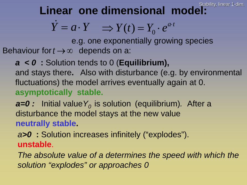
Linear one dimensional model:

a=0 : Initial valueY0 is solution (equilibrium). After a disturbance the model stays at the new value neutrally stable.

e.g. one exponentially growing species = ⋅Y a Y

Behaviour for depends on a:

t → ∞a < 0 : Solution tends to 0 (Equilibrium), and stays there. Also with disturbance (e.g. by environmental fluctuations) the model arrives eventually again at 0. asymptotically stable.

a>0 : Solution increases infinitely (“explodes”). unstable.

0( ) ⋅⇒ = ⋅ a tY t Y e

The absolute value of a determines the speed with which the solution “explodes” or approaches 0

Stability, linear multi-dim.

Linear multidimensional model

• The Eigenvalues λ of matrix A play a similar role as parameter a in the one dimensional model

11 12 1

21 22 2

1 2

n

n

n n nn

a a aa a a

Y Y A Y

a a a

= ⋅ = ⋅

nnnnnn

nn

nn

yayayay

yayayayyayayay

+++=

+++=+++=

...

......

2211

22221212

12121111

e.g. landscape transition model: y1, …, yn : landscape types, e.g. forest, pastures, fields, settlements, traffic areas, industrial areas a11, …, ann: transition probabilities (e.g. per year) between the landscape types

Stability, linear multi-dim.

Recall: Calculation of Eigenvalues

• Solution of of P(λ) = det(A - λ I) = 0, with I being the identity matrix.

• Reminder 1: • P(λ) is a polynomial of order n (dimension of

matrix) in λ and its n roots λι can be multiple as well as complex

• Reminder 2: – Complex number:

– Complex conjugate numbers: a+i b, a –i b

2 × 2 Matrix: deta11 a12

a21 a22

= a11a22 − a12a21

Real Imaginär--teil teil

a i b+ ⋅

Stability, linear multi-dim.

Meaning of Eigenvalues (λ) of A •The real parts of all λ’s are negative: equilibrium is asymptotically stable •The real parts of all λ’s are 0: equilibrium is neutrally stable. •The real part of at least one λ is positive: equilibrium is unstable. •The Eigenvalues are conjugate complex (negative argument of a square root): Oscillations

Stability, nonlinear, 1-dim

Nonlinear one dimensional model

– Ecological models are in most cases nonlinear

– Trick: in the equilibrium the right hand side is linearised (i.e. approximated by a linear function)

Stability, nonlinear, 1-dim

Linearisation • Derive the right hand side of the differential equation

with respect to the state variable – corresponds to a Taylor-series expansion, terminated after the

linear term – Taylor-series: Each function f(x) can be described by

∑∞

=

−=+−++−′′

+−′

+=0

)()(2 )(

!)(...)(

!)(...)(

!2)()(

!1)()()(

n

nn

nn

af axn

afaxn

afaxafaxafafxP

))(()()(~ mEquilibriuxmEquilibriufmEquilibriufxP −′+=

=0

)()( mEquilibriufxJ ′=Deflection from equilibrium

(Linear factor)

dxxdf a)(

Stability, nonlinear, 1-dim

Linearisation • Then go on according to the linear one

dimensional models. – Study sign of linear factor,

• negative -> stable • 0 -> neutrally stable • positive -> unstable • conjugate complex -> oscillations

• Results are valid only for equilibrium at which one has linearized !

Stability, nonlinear, 1-dim

Example for stability analysis: Logistic growth

2

( ) (1 )= = ⋅ ⋅ − = ⋅ −

Y rYY f Y Y r Y rK K

• Linearisation:

2( ) ( ) YJ Y f Y r rY K∂

= = −∂

• Equilibria:

Y1* = 0,Y2

* = K

• Substitute equilibria into linearized model:

J(0) = r − r2 ⋅ 0K

= r, J(K) = r − r2 ⋅K

K= − r

• unstable stable

Stability, nonlinear,multidim.

Nonlinear multidimensional model

• The entire “Right-hand-side-vector" is linearised at equilibrium.

• => Jacobi-Matrix – (is analogous to Matrix A

of linear models )

1 1 1

1 2

2 2 2

1 2

1 2

∂ ∂ ∂∂ ∂ ∂

∂ ∂ ∂∂ ∂ ∂

∂ ∂ ∂∂ ∂ ∂

=

n

n n n

n

Y Y YY Y YnY Y Y

J Y Y Y

Y Y YY Y Y

•Substitute equilibria •Determine Eigenvalues •Signs of real parts => stability

Stability, nonlinear,multidim.

Stability LV-competition: 21 1 21 2 1

1 1 1 1 1 1 21 1 21 1

22 2 12 1 22 2 2 2 2 2 12 1 2

2 2

( )

( )

K Y Y rY r Y Y K Y YYK K

K Y Y rY r Y Y K Y YYK K

α α

α α

− −= ⋅ ⋅ = ⋅ − −

− −= ⋅ ⋅ = ⋅ − −

Jacobi-Matrix:

J(Y *1,Y2

* ) =

r1K1

(K1 − 2Y1 −α 21Y2) −r1

K1

α21Y1

−r2

K2

α12Y2r2

K2

(K2 − 2Y2 −α12Y1)

Stability, nonlinear,multidim.

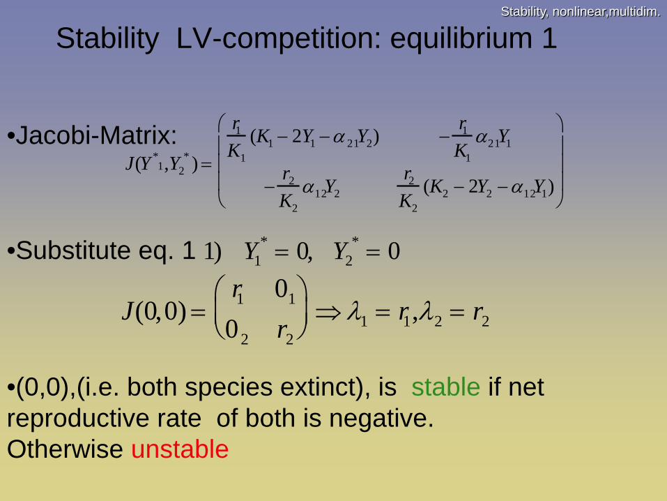
Stability LV-competition: equilibrium 1

•Jacobi-Matrix:

J(Y *1,Y2

* ) =

r1K1

(K1 − 2Y1 −α 21Y2) −r1K1

α21Y1

−r2

K2

α12Y2r2

K2

(K2 − 2Y2 −α12Y1)

•Substitute eq. 1

J(0,0) =r1 01

02 r2

⇒ λ1 = r1,λ2 = r2

•(0,0),(i.e. both species extinct), is stable if net reproductive rate of both is negative. Otherwise unstable

1) Y1* = 0, Y2

* = 0

Stability, nonlinear,multidim. Stability LV-competition,equilibria 2,3

1 2, 0 :r r >!

1 20, 0λ λ< < ⇒

•Jacobi-Matrix:

J(Y1,Y2) =

r1K1

(K1 − 2Y1 − α21Y2) −r1

K1

α 21Y1

−r2

K2

α12Y2r2

K2

(K2 − 2Y2 − α12Y1)

•Substitute eq.2 1 1 21

11 1 1 2 2 122

2 12 1 22

( ,0) , (1 )0 ( )

r rKJ K r rr K K K

K

αλ λ α

α

− − = ⇒ = − = − −

2) Y1* = K1, Y2

* = 0

•Equilibrium (K1,0),i.e. species 1 outcompetes species 2, is stable if net reproductive rate of species 1 is positive, and intraspecific competition of species 1 is smaller than the interspecific competition of species 1 to species 2. Otherwise unstable. •Analogous for equilibrium 3

1 1212

2 2 1

11KK K K

αα > ⇒ >

Stability, nonlinear,multidim.

Stability LV-competition,equilibrium 4

B: cr1(1−α21

K1K2) ⋅cr2 (1−

α12

K2K1) > cα 21r1(1−

α 21

K1K2) ⋅cα12r2(1−

α12

K2K1)

⇔ 1> α21α12 ⇒ c < 0

From conditions for stability for 2-dim. linear model

•Coexistence-equilibrium ist stable, if intraspecific competition is larger than interspecific for both species. Otherwise unstable.

J(Y *1,Y *

2) =cr1(1−

α 21

K1

K2) −cα 21r1(1−α 21

K1

K2)

−cα12r2 (1−α12

K2

K1) cr2 (1−α12

K2

K1)

,c =

1(α12α 21 −1)

21 12 21 121 2 2 1

1 2 2 1 1 2

1 1: (1 ) (1 ) 0A rc K r c K andK K K K K Kα α α α

− + − < ⇔ > >

Stability, nonlinear,multidim.

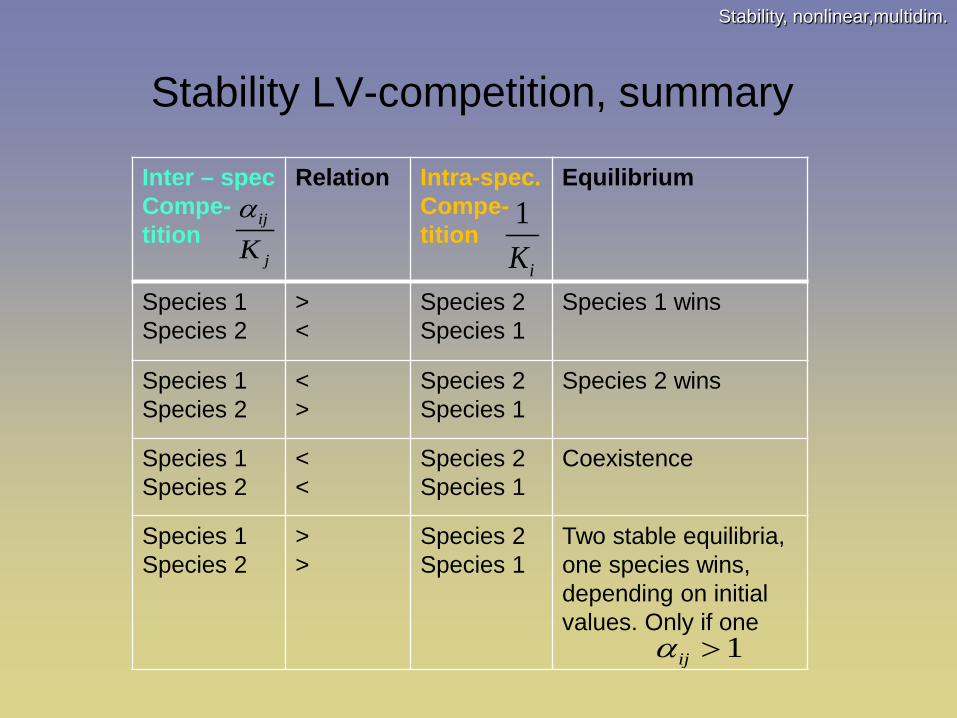
Stability LV-competition, summary

Inter – spec Compe-tition

Relation Intra-spec. Compe-tition

Equilibrium

Species 1 Species 2

> <

Species 2 Species 1

Species 1 wins

Species 1 Species 2

< >

Species 2 Species 1

Species 2 wins

Species 1 Species 2

< <

Species 2 Species 1

Coexistence

Species 1 Species 2

> >

Species 2 Species 1

Two stable equilibria, one species wins, depending on initial values. Only if one

1

iKij

jKα

1ijα >

Stabilität, zeitdiskret

Equilibrium and stability analysis for discrete time models

• Model:

X(k +1) = f (X(k))

X(k +1) = f (X(k)) = X(k)• Condition for Equilibrium: • Stability :

– 1. Linearisation of f(X(k)) – 2. Examination of Eigenvalues λ

• Absolute value of all λ <1: asymptotically stable • Absolute values of all λ = 1: (maybe) neutrally

stable • Absolute values of at least one λ >1: unstable • λ complex conjugate : Oscillation

2 2:a ib a b+ +

Absolute value of a complex number

Equilibrium and linear stability analysis in a nutshell Continuous time

Discrete time

model

equilibrium Linearisation, Jacobi-Matrix

Substitution of equilibria

Calculation of Eigenvalues λ

For stability type Eigenvalues must be

asymptotically stable

neutrally stable

instable

oscillations λ’s conjugate complex λ’s conjugate complex

0)),((!=ttyf

)),(()( 1 iii ttyfty

=+

)()( 1 ii tyty

=+

∂∂

∂∂

∂∂

∂∂

=

)()(...

)()(

:::)()(...

)()(

1

1

1

1

n

nn

n

yfyf

yfyf

yfyf

yfyf

J

0)det(!=− IJ λ

0)Re( <∀ λ0)Re( =∀ λ

0)(Re >λoneleastat

1<∀ λ1=∀ λ

1>λoneleastat

)),(()()( ttyftydt

tyd

==

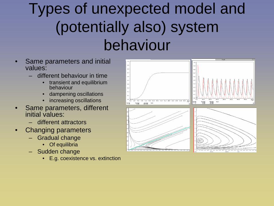
Types of unexpected model and (potentially also) system

behaviour • Same parameters and initial

values: – different behaviour in time

• transient and equilibrium behaviour

• dampening oscillations • increasing oscillations

• Same parameters, different initial values:

– different attractors • Changing parameters

– Gradual change • Of equilibria

– Sudden change • E.g. coexistence vs. extinction

Change of stability

Change of stability

Change of stability

Saturated harvesting from logistically growing stock

• model: pasture W grows logistically, eaten by R cows. But cows get saturated.

• Question: how many cows can the pasture bear?

0

(1 )

Grass Wachstum Rinderfrass

W WW r W RK W V

β

−

= ⋅ − − ⋅+

Change of stability

Saturated harvesting from logistically growing stock

• model: stock W grows logistically • harvested by R harvesters with a saturation function. • Question: how many harvesters can the stock bear? • For example W: Grass, R: cattle (fixed number)

)1(KWWrW −⋅⋅=

0VWWR+

⋅⋅− β

Change of stability

Change of equilibrium – as soon as equilibrium W3

*

appears, W1* becomes stable.

–W3* is always unstable,

– W2* always stable.

Implications • The unstable equilibrium W3

* separates the basins of attraction for the stable equilibria

W1* and W2

*. Separatrix

• The closer R gets to Rcrit2, the smaller becomes the area of attraction (“resilience”) of W2

*

• If Rcrit2 is surpassed, W2* can be reached only by decreasing R, and

lifting W above W3* . Only if R is lowered as much as to Rcrit1, W recovers

to W2* . Hysteresis

Rcrit2

Rinderbesatz R

Gra

ss W

0

3

1

2

Rcrit

V0

1

Change of stability

Equilibria

20 0

0 02 2

K V K V KV K Rr

β− − ⋅ − + − ⋅ >

0 0RVrβ

→ − <0 0KV K Rr

β ⋅→ − ⋅ <

0

(1 )

Grass Wachstum Rinderfrass

W WW r W RK W V

β

−

= ⋅ − − ⋅+

*1 0W =

2* 0 0

2,3 02 2K V K V KW V K R

rβ− − ⋅ = ± + − ⋅

equilibrium W3* becomes positive, if

equilibria W2* and W3

* disappear, i.e. the argument of the square root becomes negative for

1

0crit

V rR Rβ

→ > =

• model

⋅+

−

⋅=>→⋅+

−

>

⋅

⋅ KVVKK

rRRKVVKrKR crit 0

20

0

20

22 2 ββ

Change of stability

Stability

• linearisation

( )0

20

2(1 ) Vr W RK W V

β= − ⋅ − ⋅+

0

(1 )W WW r W RK W V

β= ⋅ − − ⋅+

( )0

20

2 W V WdW r W r RdW K W V

β+ −

= − ⋅ ⋅ − ⋅+

• model

• substitute trivial equilibrium

*1

0

( ) RW rV

βλ ⋅= −

• i.e. 0 becomes stable, when the 3rd equilibrium appears

1critR=0, 0 V rfür Rβ⋅

< >

Grenzzyklen

More strange model behaviour

Chaos

Discrete logistic model

yt +1 = yt ⋅ (1+ r ⋅ (1−yt

K))

Easy-Modelworks-Exercise:

Sample Models/Logistic growth (discr.)

Increase r from 0.1 to 2.6, note behaviour

Chaos

Discrete logistic model

yt +1 = yt ⋅ (1+ r ⋅ (1−yt

K))

r Type of equilibrium

1

1.9

2.4

2.5

2.56

2.6

3

Chaos

Discrete logistic model

yt +1 = yt ⋅ (1+ r ⋅ (1−yt

K))

r Type of equilibrium

1 Fixpoint

1.9 Dampened oscillation

2.4 2-Oscillation

2.5 4-Oscillation

2.56 8- Oscillation

2.6 Aperiodic Oscillation, Pseudo-Chaos

3 Chaos