Climate, vegetation, and predictable gradients in mammal ...sysecol2.ethz.ch/Refs/EntClim/A/An303.pdf · Climate, vegetation, and predictable gradients in mammal species richness

Climate, vegetation, and predictable gradients in mammalspecies richness in southern Africa

Peter Andrews1 and Eileen M. O'Brien2

1 Natural History Museum, London SW7 5BD, U.K.2 Institute of Ecology, University of Georgia, Athens, GA 30602, U.S.A.

(Accepted 26 July 1999)

Abstract

Many hypotheses have been proposed to account for geographic variations in species diversity. In general

these relate to some aspect of climate, particularly climatic variables measuring available or potential

energy, but while these relate directly to plant diversity they may only indirectly affect mammal species

richness. We have examined these relationships by mapping and correlating mammal species richness in

southern Africa (n = 285 species) with 15 climatic variables, two topographic variables, and woody plant

species richness (n = 1359 species). The effect of area on richness was held a constant by using an equal-area

grid cell matrix superimposed on species range maps, with each grid cell equal to 25 000 km2. We found that

variability in the plant species richness alone accounts for 75% of the variability in mammal species richness.

Of the climatic variables, only thermal seasonality approaches this ®gure, accounting for 69% of the

variability, while annual measures of temperature, precipitation or energy account for only 14±35% of

variability. Differences from North American mammal diversity studies, where annual temperature, and

hence annual potential evapotranspiration (PET), have been found to be more important, are attributed in

part to southern Africa's climate and vegetation being largely temperate to tropical, as opposed to temperate

to polar in North America. By distinguishing different types of mammal based on size, spatial and dietary

guilds, other differences emerge. Strong correlations with annual temperature exist only for large mammals,

accounting for 60±67% of the variability in species richness of large mammals compared with < 20% for

small mammals. Small mammals are strongly correlated with other climatic or vegetation parameters,

especially plant richness and thermal seasonality; frugivorous and insectivorous mammal richness is

correlated with thermal seasonality and minimum monthly PET; and arboreal and aerial species richness is

correlated with plant richness, thermal seasonality and minimum monthly PET. Up to 77% of the variability

in richness of arboreal, frugivorous and insectivorous species can be explained by woody plant richness,

compared with only 38±48% of the variability in terrestrial herbivores. It is clear from this that different

kinds of mammals are differentially affected by climatic and environmental factors, and this explains some

of the discrepancies found in earlier studies where no distinction was made between different sizes or guilds

of mammal. This result has implications both for the conservation of mammalian communities at the

present time and for understanding the evolution and structure of mammalian communities in the past.

Key words: species diversity, environment, ecology, palaeoecology

INTRODUCTION

Geographic patterns of mammal species diversity arecomplex, and several different hypotheses have beenput forward to account for them (Pianka, 1966; Begon,Harper & Townsend, 1990; Currie, 1991; Rosenzweig,1997). Generally it is assumed that climate has somecontrolling in¯uence, but exactly how is not clear, asmammals are more able to tolerate changes in climatethan other animals or sessile plants because they aremobile and warm-blooded. It is also assumed that

mammal species richness is related to vegetation(Avery, 1993), and a secondary question, therefore,concerns plant diversity: what is the relationshipbetween plant species richness patterns and vegetationstructure, and to what extent are they related tomammal diversity? It is not useful simply to relatemammal species richness to that of plants and/orhabitat, for this does not answer the fundamentalquestion about the initial causes of predictablegeographic patterns of plant or habitat diversity (e.g.Fraser, 1998; Shepherd, 1998), but it is probable that

J. Zool., Lond. (2000) 251, 205±231 # 2000 The Zoological Society of London Printed in the United Kingdom

the effects of climate on mammal diversity will beindirect, through its effects on vegetation, the source offood and shelter. This study investigates the geographicdistribution of mammal species richness in southernAfrica to identify macro-scale patterns of diversity.These are related to climatic and vegetation parametersto determine how much of the variation in mammaldiversity can be attributed to present-day variations inclimate and/or vegetation. Thus, we also describe howthe distribution of mammals might alter with changesin climate and/or vegetation.

THE STUDY AREA

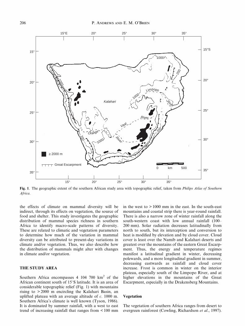
Southern Africa encompasses 4 104 700 km2 of theAfrican continent south of 158S latitude. It is an area ofconsiderable topographic relief (Fig. 1) with mountainsrising to > 2000 m encircling the Kalahari Basin, anuplifted plateau with an average altitude of c. 1000 m.Southern Africa's climate is well known (Tyson, 1986).It is dominated by summer rainfall, with a west to easttrend of increasing rainfall that ranges from < 100 mm

in the west to > 1000 mm in the east. In the south-eastmountains and coastal strip there is year-round rainfall.There is also a narrow zone of winter rainfall along thesouth-western coast with low annual rainfall (100±200 mm). Solar radiation decreases latitudinally fromnorth to south, but its interception and conversion toheat is modi®ed by elevation and by cloud cover. Cloudcover is least over the Namib and Kalahari deserts andgreatest over the mountains of the eastern Great Escarp-ment. Thus, the energy and temperature regimesmanifest a latitudinal gradient in winter, decreasingpolewards, and a more longitudinal gradient in summer,decreasing eastwards as rainfall and cloud coverincrease. Frost is common in winter on the interiorplateau, especially south of the Limpopo River, and athigher elevations in the mountains of the GreatEscarpment, especially in the Drakensberg Mountains.

Vegetation

The vegetation of southern Africa ranges from desert toevergreen rainforest (Cowling, Richardson et al., 1997).

P. Andrews and E. M. O'Brien206

15°S

20°

25°

30°

35°

15°E 20° 25° 30° 35°

15°

20°

25°

30°

35°

15° 20° 25° 30° 35°

Great Escarpment

≥ 2000 m

0 km 500

1000

200

Limpopo

1000

Kalahari

1000

1000

Orange

200 River

River

Vaal

River

200

Fig. 1. The geographic extent of the southern African study area with topographic relief, taken from Philips Atlas of Southern

Africa.

More than half of the identi®ed plant taxa for Africaoccur in southern Africa, c. 24 000 out of > 40 000identi®ed taxa. There is a longitudinal west to eastgradient in vegetation across Namibia, Botswana andSouth Africa (Gibbs Russell, 1985, 1987). In terms of¯oristic associations and af®nities, there are seven majorvegetation zones in southern Africa (White, 1981, 1983),which can be summarized brie¯y.

The north and east of the study area (other than thecoastal strip) is dominated by woodland to forest,including miombo and mopane woodland, dry ever-green forest in wetter areas, and extensive areas ofedaphic grassland. Rainfall ranges from 500 to 1400mm/year. Frosts are infrequent and localized. In thecentral and southern portions of the Kalahari basin,wooded grassland is the dominant vegetation type, withwoodland and bushland in wetter areas and open grass-land on ¯ooded or frosted areas. Rainfall is between250 and 500 mm, and frosts are widespread and severe.South of the Kalahari basin and along the west coast isdesert and bushland where rainfall rarely exceeds 250mm. Frosts are common during the winter months. TheCape ¯ora (fynbos) occupies the south-west of the studyarea. It is a characteristic Mediterranean type of lowbushland and scrubland, with rainfall con®ned to thewinter months and relatively low. Frost is infrequent toabsent. The Great Escarpment mountains of the southand east are similar in ¯oristic composition to thetropical montane regions but begin at a lower altitude.Vegetation types are extremely variable because of thetopographic relief, and they range from grassland toforest. Climate is also extremely variable, but rainfallusually exceeds 1000 mm and frosts (and snow inplaces) are frequent. The coastal forest extends alongthe east coast, and the vegetation ranges from forest totransitional woodlands and edaphic grasslands. It isextremely rich in species further north of the study area,but is relatively species-poor in Mozambique. Rainfall isbetween 800 and 1000 mm and the region is frost-free.

METHODS

Taxonomic richness

Richness is a measure of diversity that considers onlythe number of different taxa, not their relative abun-dance. At the landscape to local scales of analysis,richness varies as a function of the differential distribu-tion of individual members of taxa within theirdistributional ranges. At the macro-scale, variations inrichness are a product of the differential overlap in thedistributional ranges of taxa. Whereas ground samplingand ®eld identi®cation can be used to measure richnessat the landscape-local scales of analysis, at the macro-scale, systematic measurement of richness depends onusing distributional range maps. In either case, twoconditions are necessary for systematic analysis of rich-ness: ®rst, to avoid the confounding in¯uence of areaon the measurement of richness, area should be kept

constant through the use of equal-area sampling units;second, richness data should pertain only to ecologicallysimilar taxonomic groups (e.g. only woody plants, oronly mammals). If prediction is a goal, all relevant taxa(i.e. all mammals, all woody plants) need to be included.

Scale of analysis

The appropriate scale for analysing richness is deter-mined by the distance or area required to measurespatial heterogeneity in all variables being analysed.This study is at the macro-scale because measurableheterogeneity in climate, the independent variable,occurs over a minimum distance of 100 km (Grif®ths,1976), i.e. areas of at least 10 000 km2. Measurableheterogeneity in mammal and plant taxonomic richnessalso occurs at this scale. Based on the scale, resolutionand accuracy of the range maps, the sampling area usedhere is 25 000 km2, each cell being 1586158 km. Withinthese 25 000 km2 equal-area sampling units, woodyplant richness ranges from 6 to 567 species, from 4 to297 genera, and from 4 to 85 families (O'Brien, 1993;O'Brien, Whittaker & Field, 1998).

Mammal data

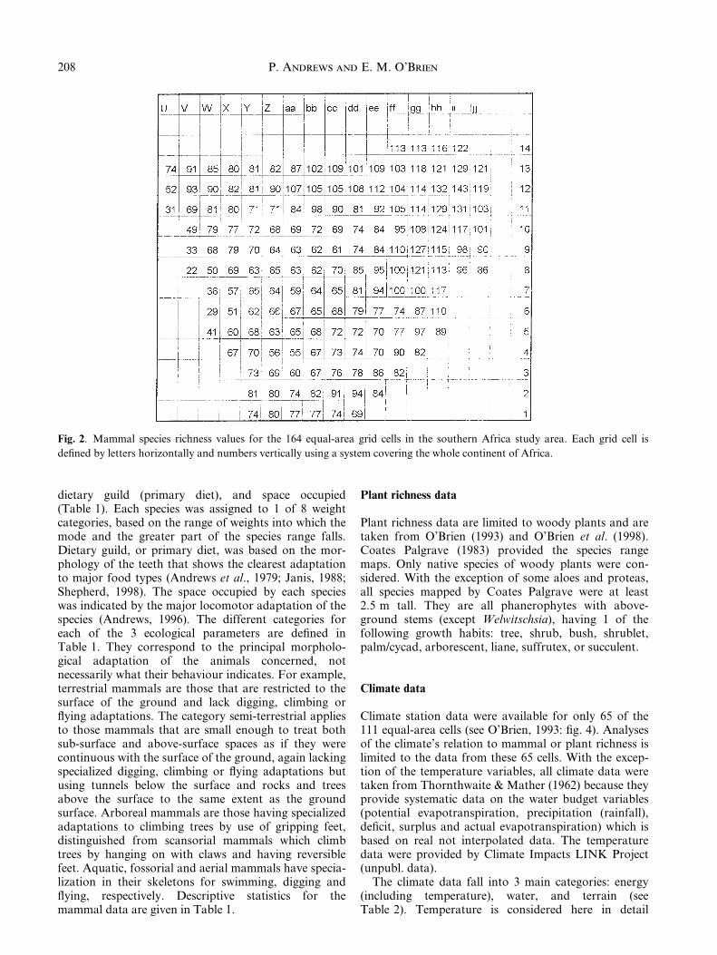
To allow systematic comparison between climate data,plant richness and mammal richness, the same metho-dology and sampling strategy employed by O'Brien(1993) to determine woody plant taxonomic richnesswas used here to determine mammal richness patterns.The same grid matrix of 164 equal-area cells was over-lain on mammal species range maps to determine thepresence or absence of a mammal species per cell (seeO'Brien, 1993: ®g. 4). The presence-absence data werethen compiled to determine the total number of species,or species richness, per cell. Only 111 cells are trulyequal-area and representative, i.e. fall entirely on landwithin the study area, and all analyses of richness dataare limited to these cells. The layout of the grid is shownin Fig. 2, the numbering and lettering of the rows andcolumns re¯ecting the fact that this is a continent-widegrid applied here just to southern Africa.

The sources of standardized range maps for southernAfrican mammals were: Smithers (1983) and Kingdon(1997), with additional data from Wilson & Reeder(1992), Frandsen (1992) and Stuart & Stuart (1988).These maps describe extant ranges for each mammalspecies, and no attempt has been made to take accountof possible human impact beyond what has been doneby the original sources. Exotic species and humans wereexcluded. There are totals of 285 mammal species (212excluding bats, which were analysed separately), 146genera and 39 families present in the study area.

Mammal richness was also examined in terms ofvarious ecological parameters. Following Andrews,Lord & Evans (1979), each species was identi®ed interms of 3 ecological parameters: body weight (size),

207Mammal species diversity in Southern Africa

dietary guild (primary diet), and space occupied(Table 1). Each species was assigned to 1 of 8 weightcategories, based on the range of weights into which themode and the greater part of the species range falls.Dietary guild, or primary diet, was based on the mor-phology of the teeth that shows the clearest adaptationto major food types (Andrews et al., 1979; Janis, 1988;Shepherd, 1998). The space occupied by each specieswas indicated by the major locomotor adaptation of thespecies (Andrews, 1996). The different categories foreach of the 3 ecological parameters are de®ned inTable 1. They correspond to the principal morpholo-gical adaptation of the animals concerned, notnecessarily what their behaviour indicates. For example,terrestrial mammals are those that are restricted to thesurface of the ground and lack digging, climbing or¯ying adaptations. The category semi-terrestrial appliesto those mammals that are small enough to treat bothsub-surface and above-surface spaces as if they werecontinuous with the surface of the ground, again lackingspecialized digging, climbing or ¯ying adaptations butusing tunnels below the surface and rocks and treesabove the surface to the same extent as the groundsurface. Arboreal mammals are those having specializedadaptations to climbing trees by use of gripping feet,distinguished from scansorial mammals which climbtrees by hanging on with claws and having reversiblefeet. Aquatic, fossorial and aerial mammals have specia-lization in their skeletons for swimming, digging and¯ying, respectively. Descriptive statistics for themammal data are given in Table 1.

Plant richness data

Plant richness data are limited to woody plants and aretaken from O'Brien (1993) and O'Brien et al. (1998).Coates Palgrave (1983) provided the species rangemaps. Only native species of woody plants were con-sidered. With the exception of some aloes and proteas,all species mapped by Coates Palgrave were at least2.5 m tall. They are all phanerophytes with above-ground stems (except Welwitschsia), having 1 of thefollowing growth habits: tree, shrub, bush, shrublet,palm/cycad, arborescent, liane, suffrutex, or succulent.

Climate data

Climate station data were available for only 65 of the111 equal-area cells (see O'Brien, 1993: ®g. 4). Analysesof the climate's relation to mammal or plant richness islimited to the data from these 65 cells. With the excep-tion of the temperature variables, all climate data weretaken from Thornthwaite & Mather (1962) because theyprovide systematic data on the water budget variables(potential evapotranspiration, precipitation (rainfall),de®cit, surplus and actual evapotranspiration) which isbased on real not interpolated data. The temperaturedata were provided by Climate Impacts LINK Project(unpubl. data).

The climate data fall into 3 main categories: energy(including temperature), water, and terrain (seeTable 2). Temperature is considered here in detail


Fig. 2. Mammal species richness values for the 164 equal-area grid cells in the southern Africa study area. Each grid cell is

de®ned by letters horizontally and numbers vertically using a system covering the whole continent of Africa.

because of its common use, especially annual tempera-ture, in faunal analyses and palaeoenvironmentalreconstructions (Crowley & North, 1991; Vrba, 1995).

Energy variables

These are based on Thornthwaite's potential evapotran-spiration (PET; Thornthwaite & Mather, 1955) andtemperature. PET is a recognized measure of the energy

regime. It describes the amount of energy available frominsolation (light) and subsequent terrestrial radiation(heat) per day, month or year. PET is empiricallyderived based on the amount of water required to meetthe environmental energy demand for evaporation andbiological processes. Because latitude is considered whencalculating PET, it also includes the effects of variableday length on the energy regime. Thornthwaite's PET,unlike other measures of PET, is not adjusted to sealevel, and thus the effect of elevation on PET is included.


Table 1. Descriptive statistics and de®nitions of taxonomic and ecological variables. nSUM, number of species in each category;n, number of grid cells analysed; X, any ecological category excluding bats

n = 65 sample n = 111 sample

Variable nSUM Mean sd Min Max Mean sd Min Max

Taxonomica

PSPECIES 1353 203.0 156.0 27 567 152.7 143.2 6 567PGENUS 450 114.4 79.7 19 297 87.4 75.2 4 297PFAMILY 110 47.1 21.0 13 83 38.1 21.3 4 85MSPECIES 285 88.1 21.0 55 143 82.7 20.7 51 143MSPECX 212 72.3 11.9 48 101 69.1 12.5 39 101MGENUS 146 69.1 12.6 47 102 65.8 12.7 41 102MFAMILY 39 31.7 3.3 25 38 31.0 3.5 21 38

Ecologicalb

Space utilizationTERR 102 45.5 7.9 32 60 45.0 7.7 23 64SEMTERR 65 19.4 3.7 12 27 18.0 3.8 12 27ARB 19 6.8 3.0 2 15 5.9 3.1 1 15SCANS 13 4.5 1.1 2 7 4.8 1.0 2 8AER 75 15.6 10.5 5 42 13.5 9.5 4 42AQ 5 2.6 1.6 0 11 2.0 1.5 0 11FOSS 25 3.8 1.0 2 6 3.8 0.9 1 6

Dietary guildINSECT 144 29.2 11.8 15 61 26.3 11.2 14 61INSECTX 79 15.6 3.8 9 24 14.5 3.8 8 26FRUG 43 11.0 3.7 3 22 10.1 3.6 3 23FRUGX 35 9.0 2.8 2 17 8.4 2.7 2 18BROW 91 20.8 2.9 15 27 20.4 2.8 15 28GRAZ 41 10.5 2.6 4 16 9.7 2.8 3 16CARN 29 17.0 2.3 12 22 16.5 2.3 10 22OMNI 7 3.4 1.2 1 6 3.3 1.3 0 6

Body sized

A 151 35.1 11.9 18 67 31.8 11.6 17 67AX 86 21.4 4.3 12 33 20.0 4.4 12 34B 45 10.4 2.6 6 20 9.7 2.4 6 20BX 37 8.4 2.3 5 15 8.0 2.0 5 15C 34 15.3 3.3 9 24 14.3 3.5 6 24D 19 11.5 2.0 7 17 10.7 2.1 5 17E 15 6.3 2.1 3 10 6.3 2.2 3 11F 4 1.4 0.6 1 3 1.5 0.6 1 4G 8 2.8 1.4 1 6 3.2 1.3 1 6H 7 4.8 0.9 2 7 4.7 1.1 1 7AB 196 45.5 13.8 25 87 41.6 13.4 24 87ABC 230 60.9 16.5 36 108 55.9 16.4 36 108ABCD 249 72.4 18.0 44 120 66.7 18.0 43 120EFGH 34 15.6 4.6 9 24 15.9 4.4 7 27FGH 19 9.2 2.6 6 15 9.6 2.5 4 17

a PSPECIES, woody plant species richness; PGENUS, woody plant genus richness; PFAMILY, woody plant family richness;MSPECIES, mammal species richness; MSPECX, mammal species richness excluding bats; MGENUS, mammal genus richness;MFAMILY, mammal family richness.b T, Terrestrial; B, semi-arboreal; A, arboreal; S, scansorial; Aq, aquatic; F, fossorial; R, aerial.c I, Insectivory; F, frugivory; B, browsing; G, grazing; C, carnivory; O, omnivory.d A, 0±100g; B, 100 g±1 kg; C, 1±10 kg; D, 10±45 kg; E, 45±90 kg; F, 90±180 kg; G, 180±360 kg; H, > 360 kg.

When PET is combined with information on the actualamount of water available to meet the environmentaldemand, it is possible to determine AET, the actualevapotranspiration or the amount of water that canactually be used for evaporation and biological pro-cesses at any given place or time. Average minimum andmaximum monthly PET (PEMIN and PEMAX), therange between them, or seasonal variability in the energyregime (DIFPE), and average annual PET (PEAN) areexamined.

Temperature is a partial index of the environmentalenergy regime. It describes the degree of heat. It is not ameasure of day length, nor of the total amount orduration of heat. Thus, monthly and annual tempera-ture values only describe the average daily degree ofheat per month or year. Average minimum (TMIN) andmaximum (TMAX) monthly temperature, the rangebetween them, or thermal seasonality (DIFT), andaverage annual temperature (TAN) are examined.

Water variables

Precipitation is the main water variable considered. It is aprimary, albeit partial, measure of the water available tomeet the environmental demand for water, soil moisturenot being included. Annual, maximum and minimummonthly precipitation, and the range between them(PAN, PMAX, PMIN and DIFP, respectively) are con-sidered, as well as several other water variables. Theseare: (1) annual AET (AEAN, see above), which inaddition to providing information on the effectivemoisture regime, is a recognized proxy for net primary

productivity and biological activity (cf. Rosenzweig,1968); (2) Thornthwaite's moisture index (PMI), which isan index of the effective moisture regime that is used inthe classi®cation of vegetation in southern Africa; (3) theduration of the dry season (DRY), i.e. number of monthswith zero precipitation; and (4) the duration of thegrowing season (RAINS), i.e. the number of monthswith at least 25 mm rainfall (cf. Schulze & McGee, 1977).

Terrain variables

These are elevation (ELEV) and topographic relief(TOPOG). Both variables are directly related to varia-bility in climate. Changes in elevation cause predictablechanges in temperature (� 6.58 per 1 km). Changes intopographic relief cause adiabatic cooling and heatingof air forced to rise and fall (� 5±10 8C/km) as varia-bility in elevation changes, and this produces orographicrainfall/cloud cover and/or rainshadows. Topographicrelief is de®ned here as the range between the minimumand maximum elevation per cell (> 90 samples per cell).It does not take into account the number of times theelevation changes within a cell, or lesser changes inheight, i.e. those changes less than the maximumchange. Although elevation is often considered a reason-able proxy for topographic relief, these 2 variables arenot signi®cantly correlated with each other at themacro-scale. This is reasonable when we consider thattopographic relief can be low at both high and lowelevations (e.g. elevated plateaux and coastal plains,respectively). Major variations in elevation andtopographic relief for the study area are shown in Fig. 1.


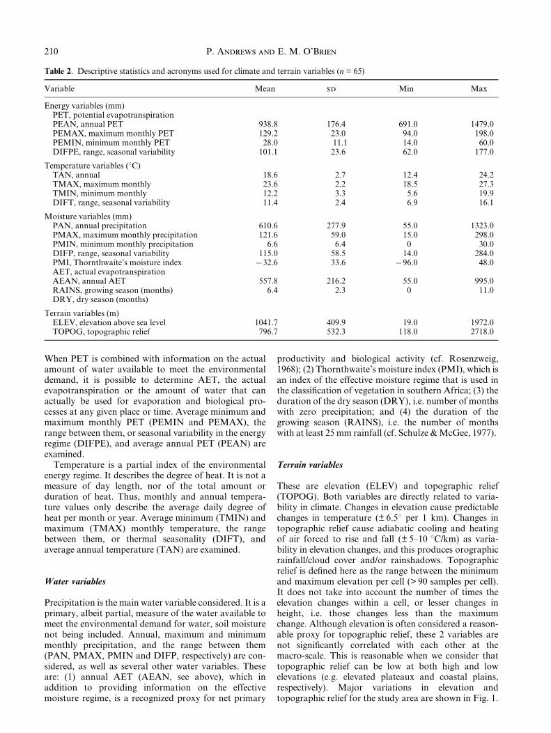
Table 2. Descriptive statistics and acronyms used for climate and terrain variables (n = 65)

Variable Mean sd Min Max

Energy variables (mm)PET, potential evapotranspirationPEAN, annual PET 938.8 176.4 691.0 1479.0PEMAX, maximum monthly PET 129.2 23.0 94.0 198.0PEMIN, minimum monthly PET 28.0 11.1 14.0 60.0DIFPE, range, seasonal variability 101.1 23.6 62.0 177.0

Temperature variables (8C)TAN, annual 18.6 2.7 12.4 24.2TMAX, maximum monthly 23.6 2.2 18.5 27.3TMIN, minimum monthly 12.2 3.3 5.6 19.9DIFT, range, seasonal variability 11.4 2.4 6.9 16.1

Moisture variables (mm)PAN, annual precipitation 610.6 277.9 55.0 1323.0PMAX, maximum monthly precipitation 121.6 59.0 15.0 298.0PMIN, minimum monthly precipitation 6.6 6.4 0 30.0DIFP, range, seasonal variability 115.0 58.5 14.0 284.0PMI, Thornthwaite's moisture index 732.6 33.6 796.0 48.0AET, actual evapotranspirationAEAN, annual AET 557.8 216.2 55.0 995.0RAINS, growing season (months) 6.4 2.3 0 11.0DRY, dry season (months)

Terrain variables (m)ELEV, elevation above sea level 1041.7 409.9 19.0 1972.0TOPOG, topographic relief 796.7 532.3 118.0 2718.0

Statistical analyses and model development

Statistical analyses were performed using a variety ofSAS programs for descriptive statistics correlation,analysis of variance and linear or multiple regression.For model development, SAS regression procedure,RSQUARE, was used to describe the n most powerful1-, 2-, and 3-variable regression models of mammal

species, genus and family richness. The criteria used toselect which of the generated models 'best' describe howrichness and/or climate relate to mammal richness were:(1) explanatory power (coef®cient of determination r2 );(2) simplicity (least number of variables);(3) maximum level of precision (low root mean squareerror, RMSE);(4) parsimony (least number of assumptions).


15°

20°

25°

30°

35°

15° 20° 25° 30° 35°

15°

20°

25°

30°

35°

15° 20° 25° 30° 35°

0 km 500

<1<1 5 10

20 30

20

4030

15°

20°

25°

30°

35°

15° 20° 25° 30° 35°

15°

20°

25°

30°

35°

15° 20° 25° 30° 35°

0 km 500

15

1020

35

25

40

30

20

4550

(a) (b)

(d) West–east transect

Woody plants

Total mammals

600

500

400

300

200

100

0

U11

V11

X11

Y11

Z11

aa11

bb11

cc11

dd11

ee11 ff11

gg11

hh11 ii11

Grid cells

(c) South–north transect

Woody plants

Total mammals

450

350

400

300

200

100

0

ff4 ff5 ff6 ff7 ff8 ff9 ff10

ff11

ff12

gg13

Grid cells

50

150

250

No.

of s

peci

es

30

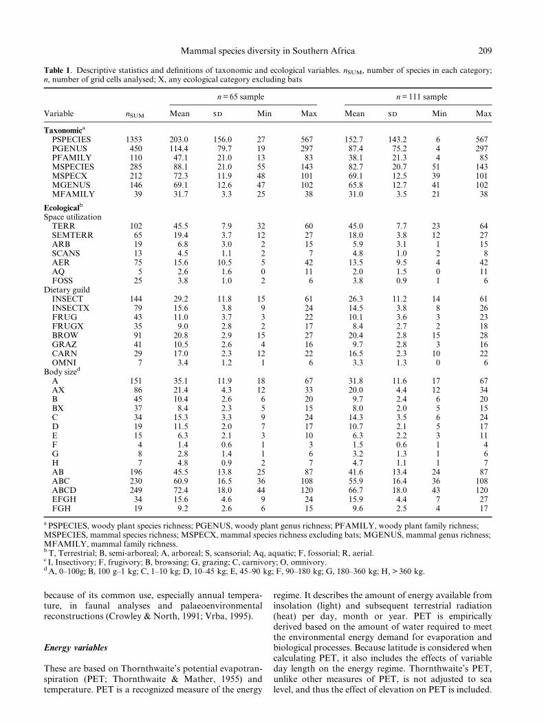
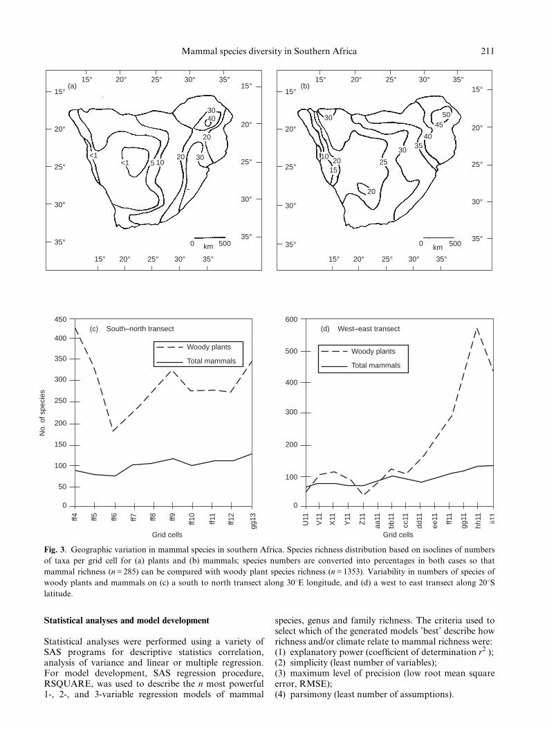
Fig. 3. Geographic variation in mammal species in southern Africa. Species richness distribution based on isoclines of numbers

of taxa per grid cell for (a) plants and (b) mammals; species numbers are converted into percentages in both cases so that

mammal richness (n = 285) can be compared with woody plant species richness (n = 1353). Variability in numbers of species of

woody plants and mammals on (c) a south to north transect along 308E longitude, and (d) a west to east transect along 208Slatitude.

To reduce the potential for multicollinearity amongstthe independent variables, only 1 each of the energy,water, or terrain variables was allowed in a model ofclimate's relation to richness. Models of mammal rich-ness based on vegetation parameters could onlycombine plant richness with temperature and/or terrainvariables (all other variables being inherent in plantrichness). No grid cells were removed as outliers, theassumption being that the unexplained variance is morelikely to be a function of missing variables than ofmis-measurement.

The results are presented in the following sequence:(1) mammal taxonomic richness and how it relates toplant taxonomic richness based on the full sample of111 grid cells, i.e. those cells that do not extend overland or sea boundaries; (2) how temperature relates toother climate variables, and how all climate variablesrelate to mammal or plant richness, based on thesmaller sample of 65 grid cells with climate stations; (3)how ecological subsets of mammal richness relate toeach other, to all-mammal and plant richness (n = 111),and to climate (n = 65). The signi®cance level of allstatistical results presented in text is P < 0.0001, unlessotherwise indicated.

RESULTS

Geographic patterns in mammal richness in relation tovegetation

The variation in numbers of mammals per grid cellacross southern Africa is illustrated in Fig. 2, and thepattern of mammal species richness is shown in Fig. 3bas isoclines of species numbers per grid cell. There isonly a weak latitudinal gradient of increase in numbersof mammal species from the south of the study area tothe north (Fig. 3b,c). By contrast, the woody plant


Table 3. Taxonomic relations: mammal±plant richness. Pearson's product moment correlations. P < 0.0001. Abbreviations as inTable 1

PSPECIES PGENUS PFAMILY MSPECIES MSPECX MGENUS MFAMILY

A (n = 111)PSPECIES 0 0.9936 0.9288 0.8653 0.8216 0.8350 0.7043PGENUS 0.9936 0 0.9405 0.8772 0.8313 0.8479 0.7110PFAMILY 0.9288 0.9405 0 0.7777 0.7672 0.7625 0.6227MSPECIES 0.8653 0.8772 0.7777 0 0.9546 0.9860 0.8861MSPECX 0.8216 0.8313 0.7672 0.9546 0 0.9644 0.8975MGENUS 0.8350 0.8479 0.7625 0.9860 0.9644 0 0.9130MFAMILY 0.7043 0.7110 0.6227 0.8861 0.8975 0.9130 0

B (n = 65)PSPECIES 0 0.9925 0.9216 0.7243 0.7345 0.7030 0.5932PGENUS 0.9925 0 0.9373 0.7358 0.7488 0.7191 0.5977PFAMILY 0.9216 0.9373 0 0.6047 0.6768 0.5987 0.4788MSPECIES 0.7244 0.7358 0.6047 0 0.9450 0.9869 0.8853MSPECX 0.7345 0.7488 0.6768 0.9450 0 0.9498 0.8619MGENUS 0.7030 0.7191 0.5987 0.9869 0.9497 0 0.8993MFAMILY 0.5932 0.5977 0.4788 0.8853 0.8619 0.8993 0

Table 4. Correlations of temperature variables with eachother and with other climate variables. Abbreviations as inTable 2. n = 65; P < 0.0001; NS = not signi®cant if P > 0.01

TMAX TMIN DIFT TAN

TMAX 1.00000 0.67858 0.862480.0 0.0001 NS 0.0001

TMIN 0.67858 1.00000 70.73948 0.947320.0001 0.0 0.0001 0.0001

DIFT 70.73948 1.00000 70.49922NS 0.0001 0.0 0.0001

TAN 0.86248 0.94732 70.49922 1.000000.0001 0.0001 0.0001 0.0

PEMAX 0.74249 0.38263 0.530410.0001 0.0017 NS 0.0001

PEMIN 0.34141 0.85415 70.84994 0.686430.0054 0.0001 0.0001 0.0001

DIFPE 0.56204 0.557410.0001 NS 0.0001 NS

PEAN 0.76532 0.80696 70.39717 0.834880.0001 0.0001 0.0011 0.0001

PMAX 0.48110 70.73954NS 0.0001 0.0001 NS

PMIN 70.41572 70.342610.0006 NS NS 0.0052

DIFP 0.50212 70.72695 0.34979NS 0.0001 0.0001 0.0043

PAN 70.67217NS NS 0.0001 NS

AEAN 0.32068 70.66907NS 0.0092 0.0001 NS

PMI 70.56975 70.451550.0001 NS 0.0002 NS

RAINS 70.348860.0044 NS NS NS

ELEV 70.46977 70.55902 0.33051 70.503550.0001 0.0001 0.0072 0.0001

TOPOG 70.65118 70.445910.0001 NS NS 0.0002

richness does not show a clear trend latitudinally. Fromwest to east, the dominant pattern is longitudinal, witha trend of increasing richness in both plant andmammal species that is greater for the plants than forthe mammals (Fig. 3d). The Namibian coast has thelowest mammal richness extending eastwards into theKalahari. The highest mammal richness occurs in theZambezi forests of Zimbabwe, Mozambique and SouthAfrica, along the highlands of the eastern Great Escarp-ment, as well as the eastern coast, and these are also theareas of highest plant species richness.

The geographic pattern of variation in mammalrichness is similar at all taxonomic levels. Whennumbers of genera are plotted in the same way, thedistribution is nearly identical to that for species, butbecause of the comparatively small number of families(39) and their small range of variation (21±38 familiesper cell), this trend is less obvious. The similarities inmammal distribution are supported by high correlations(Table 3): r = 0.986 between species and genus; r = 0.913between genus and family; and r = 0.886 between speciesand family. Similarly strong correlations also occur forthe subset of 65 cells with climate station data (Table 3).

Correlations between plant species richness andmammal richness range from r = 0.704 for mammalfamily richness to r = 0.865 for mammal species richness(Table 3). Similar patterns and correlations occurbetween plant genus/family richness and mammal rich-ness at all taxonomic levels, although the correlationsbetween plant family richness and mammal richness areweaker. In all cases the correlations between plant andmammal richness for the sample of 65 cells that haveclimate data are weaker. For example, for plant/mammal at n = 111, r = 0.865 compared with r = 0.724for n = 65. This suggests that some factor affects plantand mammal richness in the 65 grid cell subset differ-ently from the whole set of 111 equal-area cells, and onesuch factor could be terrain.

How temperature relates to other climate variables

The correlations among temperature parameters, andbetween them and the other climate variables are pre-sented in Table 4. Annual temperature seems to be anambiguous measure of the climate regime, and the mostcritical temperature variables are minimum monthlytemperature (TMIN) and the difference betweenmaximum and minimum monthly temperatures (DIFT).These are both measures of thermal seasonality,whereas annual temperature can be the same whetherthe monthly temperature is the same year-round orhighly seasonal. Thermal seasonality (DIFT) insouthern Africa is most strongly correlated withchanges in minimum monthly potential evapotranspira-tion (PEMIN, r = 0.850) as well as with minimummonthly temperature (TMIN, r =70.740).

Thermal seasonality (DIFT) is also the temperaturevariable most strongly correlated with variations in thewater variables (Table 4), especially those shown to bestrongly correlated with plant richness (Table 5). Thewater variables most highly correlated with thermalseasonality are maximum monthly precipitation(PMAX, r =70.739) and the difference betweenmaximum and minimum monthly precipitation (DIFP,r =70.726). These variables are greatest when thermalseasonality is least. By contrast, annual temperature isonly weakly correlated with two of the water variables, sothat in effect, changes in annual temperature are ambig-uous or poor indicators of changes in the rainfall regime.Consistent with how elevation affects air temperature,the terrain variables tend to be weakly and negativelycorrelated with all temperature variables (Table 4).

How climate variables relate to mammal and woodyplant richness

The climate variables most strongly correlated with


Table 5. Correlations between plant and mammal richness and climate. Abbreviations as in Table 1. n = 65; P < 0.0001, unlessotherwise indicated: ** = P < 0.001, * = P < 0.01; NS = not-signi®cant when P > 0.01


PEMAX 70.356* 70.343* 70.502 NS NS NS NSPEMIN 0.617 0.655 0.470 0.712 0.669 0.741 0.676DIFPE 70.639 70.644 70.711 70.421 70.473 70.418** 70.377*PEAN NS NS NS 0.375* 0.319* 0.403** 0.397**TMAX NS NS 70.475 NS NS NS NSTMIN 0.413** 0.428** NS 0.702 0.627 0.714 0.715DIFT 70.798 70.821 70.689 70.830 70.794 70.835 70.734TAN NS NS NS 0.530 0.460 0.541 0.598PMAX 0.750 0.761 0.671 0.740 0.737 0.725 0.584PMIN 0.335* 0.387* 0.486 NS NS NS NSDIFP 0.719 0.723 0.622 0.741 0.732 0.726 0.598PAN 0.775 0.795 0.778 0.593 0.649 0.579 0.422**AEAN 0.701 0.731 0.711 0.532 0.601 0.539 0.434**PMI 0.662 0.669 0.741 0.391* 0.468 0.368* NSRAINS 0.458 0.490 0.573 NS NS NS NSELEV NS NS NS NS NS NS NSTOPOG 0.580 0.585 0.678 NS NS NS NS

mammal richness in southern Africa are those de-scribing seasonal variability (Table 5): maximummonthly rainfall (PMAX), rainfall seasonality (DIFP),minimum monthly PET (PEMIN) and the seasonaltemperature variables DIFT and TMIN. This is consis-tent with the study area being dominated by summerrainfall that can last from < 1 month to > 7 months. Ineffect mammal richness tends to be greatest whereseasonal variability in the water regime is least. Here thediversity of food resources (plant richness) and theiramount and duration (i.e. productivity or annual AET)are greatest, and as seasonal variability in the waterregime increases, the diversity, amount and duration offood resources tend to decrease. The terrain variablesare signi®cantly correlated to only plant richness. Theweak correlation with mammal richness suggests thatchanges in elevation or topographic relief are unlikely toaffect mammal richness unless this is associated withchanges in the vegetation.

The weak or insigni®cant correlations between annualmeasures of the energy regime and mammal/plantrichness and the other climate variables (Table 5)further emphasize the importance of climatic season-ality. The energy regime, as de®ned by annual potentialevapotranspiration (PET) and annual temperature(TAN) is not signi®cantly correlated with plant richness

(P > 0.01) and is only weakly correlated with mammalrichness (r < 0.598).

Correlations of ecological subsets of mammal speciesrichness

Most analyses of mammal species richness considermammal faunas as a whole (for an exception see Shep-herd, 1998), but it is probable that different types ofmammal would interrelate with climatic variables todifferent degrees. We have therefore examined speciesrichness patterns for different categories of mammalsaccording to body size and spatial and dietary guilds.Some of these ecological subsets have few species (< 15species) with little variation per cell (Table 1), andsometimes we have combined classes of mammals,particularly different size classes. Correlations withclimate variables are shown in Table 6, and to investi-gate these patterns in terms of geographic distributions,we have mapped species numbers as isoclines on thesame scale as for total diversity but subdivided intoecological categories. The isoclines are based on percen-tage numbers of species to make the maps comparableone with another and with Fig. 3.


Table 6. Pearson's product moment correlations between ecological and climate variables. n = 65; P < 0.0001 unless otherwise

Energy variables Temperature

PEMAX PEMIN DIFPE PEAN TMAX TMIN DIFT TAN

Ecological categoriesSpace utilization

TERR NS 0.68535 70.34859* 0.45184** NS 0.74958 70.73027 0.64532SEMTERR 70.47639 NS 70.48031 NS 70.47166 NS NS NSARB NS 0.70728 70.38496* 0.38779* NS 0.64677 70.79422 0.47377SCANS NS NS NS NS 0.38200* NS NS 0.35489*AER NS 0.66712 NS 0.39241* NS 0.69578 70.76002 0.54113AQ NS NS NS NS 70.35203* NS NS NSFOSS NS 70.42940** NS 70.44833* 70.38786* 70.52042 0.35302** 70.50626

Dietary guildsINSECT NS 0.60226 70.40344** NS NS 0.62821 70.77082 0.46380INSECTX 70.37884* NS 70.48435 NS NS NS 70.52604 NSFRUG NS 0.72015 70.37068* 0.41239** NS 0.66326 70.81213 0.48177FRUGX NS 0.66965 70.40024** 0.35807* NS 0.60483 70.76926 0.43870**BROW NS 0.50659 70.36065* NS NS 0.49282 70.58215 0.36533*GRAZ NS 0.54461 70.37487* NS NS 0.4187** 70.60668 NSCARN NS 0.53925 NS 0.36670* NS 0.53229 70.54389 0.45310**OMNI NS 0.70105 NS 0.47526 0.35518* 0.70457 70.63367 0.59420

Body sizeA NS 0.59722 70.42018** NS NS 0.58896 70.77234 0.40957**AX 70.38982* NS 70.48178 NS 70.35636* NS 0.44867** NSB NS 0.50694 NS NS NS 0.4483** 70.51392 0.34364*BX NS NS NS NS NS NS NS NSC NS 0.59042 70.47610 NS NS 0.54898 70.73578 0.38165*D NS 0.51713 70.40036** NS NS 0.32905* 70.60593 NSE NS 0.69075 NS 0.57295 0.51587 0.81841 70.64138 0.76999F NS 0.66865 NS 0.64892 0.45471 0.73517 70.58411 0.68406G NS 0.59017 NS 0.51786 0.45354 70.55808 0.67149 0.39507*H NS 0.59242 NS 0.50743 0.45082** 0.67143 70.50091 0.63938

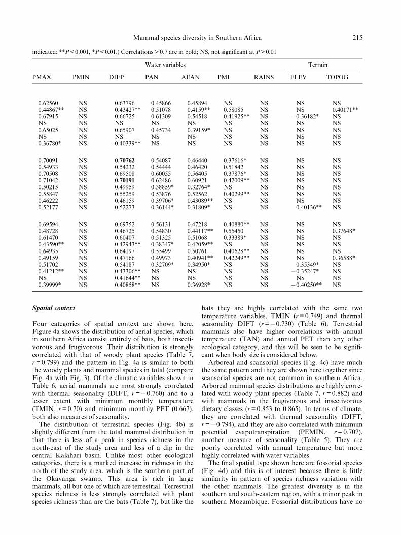
Spatial context

Four categories of spatial context are shown here.Figure 4a shows the distribution of aerial species, whichin southern Africa consist entirely of bats, both insecti-vorous and frugivorous. Their distribution is stronglycorrelated with that of woody plant species (Table 7,r = 0.799) and the pattern in Fig. 4a is similar to boththe woody plants and mammal species in total (compareFig. 4a with Fig. 3). Of the climatic variables shown inTable 6, aerial mammals are most strongly correlatedwith thermal seasonality (DIFT, r =70.760) and to alesser extent with minimum monthly temperature(TMIN, r = 0.70) and minimum monthly PET (0.667),both also measures of seasonality.

The distribution of terrestrial species (Fig. 4b) isslightly different from the total mammal distribution inthat there is less of a peak in species richness in thenorth-east of the study area and less of a dip in thecentral Kalahari basin. Unlike most other ecologicalcategories, there is a marked increase in richness in thenorth of the study area, which is the southern part ofthe Okavanga swamp. This area is rich in largemammals, all but one of which are terrestrial. Terrestrialspecies richness is less strongly correlated with plantspecies richness than are the bats (Table 7), but like the

bats they are highly correlated with the same twotemperature variables, TMIN (r = 0.749) and thermalseasonality DIFT (r =70.730) (Table 6). Terrestrialmammals also have higher correlations with annualtemperature (TAN) and annual PET than any otherecological category, and this will be seen to be signi®-cant when body size is considered below.

Arboreal and scansorial species (Fig. 4c) have muchthe same pattern and they are shown here together sincescansorial species are not common in southern Africa.Arboreal mammal species distributions are highly corre-lated with woody plant species (Table 7, r = 0.882) andwith mammals in the frugivorous and insectivorousdietary classes (r = 0.853 to 0.865). In terms of climate,they are correlated with thermal seasonality (DIFT,r =70.794), and they are also correlated with minimumpotential evapotranspiration (PEMIN, r = 0.707),another measure of seasonality (Table 5). They arepoorly correlated with annual temperature but morehighly correlated with water variables.

The ®nal spatial type shown here are fossorial species(Fig. 4d) and this is of interest because there is littlesimilarity in pattern of species richness variation withthe other mammals. The greatest diversity is in thesouthern and south-eastern region, with a minor peak insouthern Mozambique. Fossorial distributions have no


indicated: **P < 0.001, *P < 0.01.) Correlations > 0.7 are in bold; NS, not signi®cant at P > 0.01

Water variables Terrain

PMAX PMIN DIFP PAN AEAN PMI RAINS ELEV TOPOG

0.62560 NS 0.63796 0.45866 0.45894 NS NS NS NS0.44867** NS 0.43427** 0.51078 0.4159** 0.58085 NS NS 0.40171**0.67915 NS 0.66725 0.61309 0.54518 0.41925** NS 70.36182* NSNS NS NS NS NS NS NS NS NS0.65025 NS 0.65907 0.45734 0.39159* NS NS NS NSNS NS NS NS NS NS NS NS NS

70.36780* NS 70.40339** NS NS NS NS NS NS

0.70091 NS 0.70762 0.54087 0.46440 0.37616* NS NS NS0.54933 NS 0.54232 0.54444 0.46420 0.51842 NS NS NS0.70508 NS 0.69508 0.60055 0.56405 0.37876* NS NS NS0.71042 NS 0.70191 0.62486 0.60921 0.42009** NS NS NS0.50215 NS 0.49959 0.38859* 0.32764* NS NS NS NS0.55847 NS 0.55259 0.53876 0.52562 0.40299** NS NS NS0.46222 NS 0.46159 0.39706* 0.43089** NS NS NS NS0.52177 NS 0.52273 0.36144* 0.31809* NS NS 0.40136** NS

0.69594 NS 0.69752 0.56131 0.47218 0.40880** NS NS NS0.48728 NS 0.46725 0.54830 0.44117** 0.55450 NS NS 0.37648*0.61470 NS 0.60407 0.51325 0.51068 0.33389* NS NS NS0.43590** NS 0.42943** 0.38347* 0.42059** NS NS NS NS0.64935 NS 0.64197 0.55499 0.50761 0.40628** NS NS NS0.49159 NS 0.47166 0.49973 0.40941** 0.42249** NS NS 0.36588*0.51702 NS 0.54187 0.32709* 0.34950* NS NS 0.35349* NS0.41212** NS 0.43306** NS NS NS NS 70.35247* NSNS NS 0.41644** NS NS NS NS NS NS0.39999* NS 0.40858** NS 0.36928* NS NS 70.40250** NS

signi®cant correlation with overall mammal or woodyplant distributions (Table 7), and correlations with allother ecological classes are non-signi®cant (Table 6). Ofparticular interest, however, is that the fossorial speciesrichness pattern is negatively correlated at low levels ofsigni®cance with most climate variables with the excep-tion of DIFT (Table 6). Thermal seasonality has beenseen above to be strongly negatively correlated withmost aspects of plant and mammal richness patterns,but it is positively correlated with fossoriality (Table 6,r = 0.353, P < 0.001). This is a low level of probabilitycompared with most other aspects of this analysis, but itis accepted here as a genuine re¯ection of an importantaspect of the fossorial adaptation, namely association

with seasonal environments with their greater abun-dance of geophytes and hemicryptophytes, whichprovide an important food source for fossorial vegetar-ians. Other than this, the distribution of fossorialspecies is probably linked with soil type, which we havenot analysed in the present work.

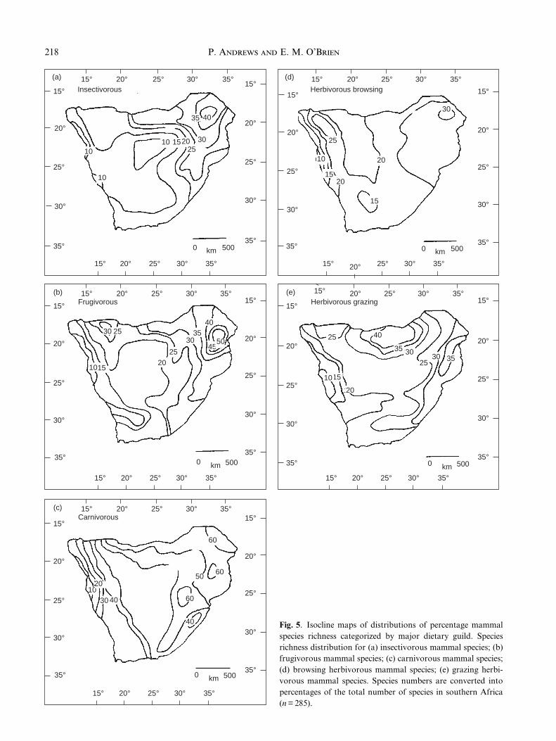
Diet

Several of the dietary classes show patterns differingfrom the general mammalian pattern, and they make aninteresting comparison with those that are similar.Figures 5a & 5b show the distributions of insectivorous


15°

20°

25°

30°

35°

15° 20° 25° 30° 35°15°

20°

25°

30°

35°

15° 20° 25° 30° 35°

20

30

40

(c)

10

15

60

50

35

Arboreal/scansorial

15°

20°

25°

30°

35°

15° 20° 25° 30° 35°

15°

20°

25°

30°

35°

15° 20° 25° 30° 35°

0 km 500

(d)Fossorial

0 km 500

30

10

5

15

10

10

10

15

15

15

10

20

20

15°

20°

25°

30°

35°

15° 20° 25° 30° 35°15°

20°

25°

30°

35°

15° 20° 25° 30° 35°

520

30

40

(a)

10

10 15

555045

35

Aerial

15°

20°

25°

30°

35°

15° 20° 25° 30° 35°

15°

20°

25°

30°

35°

15° 20° 25° 30° 35°

0 km 500

20

55 60

4045

50

(b)

30

Terrestrial

55

40

5045

0 km 500

Fig. 4. Isocline maps of distributions of percentage mammal species richness categorized by spatial distribution. Species richness

distribution for (a) ¯ying (aerial) mammal species; (b) terrestrial mammal species; (c) tree-living (arboreal and scansorial)

mammal species; (d) mammals with fossorial adaptations. Species numbers are converted into percentages of the total number of

species in southern Africa (n = 285).

and frugivorous mammal species, respectively, andthese both conform to the general pattern for mammals.Both are strongly correlated with distributions of ar-boreal and aerial species distributions (Table 6, r = 0.853to 0.962), and the relationship is shown here inFig. 6a±c. These combinations of off-the-ground spaceutilization with frugivory and insectivory are highlydependent on woody plant species richness patterns(Table 7, r = 0.82 to 0.85, although excluding batsr = 0.74 to 0.76). Like the plants also, the distributionsof insectivores and frugivores are strongly correlatedwith thermal seasonality (Table 6, DIFT, r =70.769 to70.812) and to a slightly lesser degree with moisturevariables maximum monthly precipitation (PMAX) andrainfall seasonality (DIFP).

It was unexpected to ®nd the distribution ofinsectivorous mammals so similar to that of woodyplants and with the highest correlation of any dietarytype (Table 7). Insectivores are secondary consumers ata higher level in the food chain than the insects they areeating, and it would seem that this similarity is the resultof both the limited ranges of vegetation types to whichthe insects are adapted and the limited diversity ofinsects that the mammalian insectivores are eating. Arather different pattern emerges when carnivorousmammals are analysed separately (Fig. 5c). Carnivoresare at least another level up the food chain and have nodirect interaction with plants, and not surprisingly theirdistribution is less tied in to that of plants or othermammals. Rather more surprising is that carnivoreshave such a poor relationship with their prey, at least interms of species richness per equal-area grid cell, andthis is shown in Fig. 6d, which relates carnivore speciesrichness to that of browsing herbivores. In fact carnivoredistribution is more strongly longitudinal than those ofother mammals and it ignores the change to winterrainfall in the Cape region. Species richness of carni-vores increases rapidly eastwards from the western partof the study area, so that even the Kalahari region hasnearly 50% of the southern African carnivore species.Their pattern of distribution is moderately correlated

with several climatic variables (Table 6) but not stronglyso with any single variable, and the only ecologicalparameter they are correlated with is terrestrialism(Table 6, r = 0.751). They have the lowest correlationwith vegetation of any dietary type (Table 7).

Browsing and grazing herbivores have distributionpatterns that are both different from each other anddifferent from other mammals (Fig. 5d, e). Even thecorrelation of browsers with numbers of carnivores pergrid cell was not pronounced (Fig. 6d). Over most of thestudy region, at least 20% of both the 91 browsers and 41grazers are present, whereas < 20% of insectivores arepresent over large parts of the western two-thirds of theregion. This means that these herbivore species havebroader distributional ranges that encompass withinthem wider ranges of vegetation types than mammalsthat have insectivorous or frugivorous diets. Like thecarnivores, however, the browsers and grazers are onlymoderately correlated with climate variables and notstrongly with any one variable (Table 6), and they arenot as strongly correlated with plant species distributionsas are frugivores and insectivores, although they aremore strongly correlated than the carnivores (Table 7).They are correlated with terrestrial space use, and bothhave distribution peaks in the north of the study area (ashas been seen for terrestrial mammals) where it passesinto the Okavanga delta region. This is particularlymarked in the case of grazing mammals, and it is theonly part of southern Africa with a suf®cient variety ofresources to support three species of alcelaphine ante-lope. In general, browsers and grazers lack strongcorrelations with any one climatic variable (Table 6),and they are less highly correlated with vegetation thanare frugivores and insectivores (Table 7).

Body size

Many of the distributions of ecological classes areknown to be strongly size-related. For example insecti-vorous and aerial species are mostly small, frugivorous


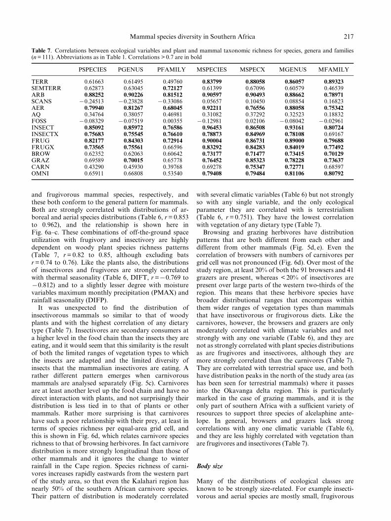
Table 7. Correlations between ecological variables and plant and mammal taxonomic richness for species, genera and families(n = 111). Abbreviations as in Table 1. Correlations > 0.7 are in bold


TERR 0.61663 0.61495 0.49760 0.83799 0.88058 0.86057 0.89323SEMTERR 0.62873 0.63045 0.72127 0.61399 0.67096 0.60579 0.46539ARB 0.88252 0.90226 0.81512 0.90597 0.90493 0.88662 0.78971SCANS 70.24513 70.23828 70.33086 0.05657 0.10450 0.08854 0.16823AER 0.79940 0.81267 0.68045 0.92211 0.76556 0.88058 0.75342AQ 0.34764 0.38057 0.46981 0.31082 0.37292 0.32523 0.18832FOSS 70.08329 70.07519 0.00355 70.12981 0.02106 70.08042 70.02961INSECT 0.85092 0.85972 0.76586 0.96453 0.86508 0.93161 0.80724INSECTX 0.75683 0.75545 0.76610 0.78873 0.84969 0.78108 0.69167FRUG 0.82177 0.84303 0.72914 0.90004 0.86731 0.89000 0.79688FRUGX 0.73565 0.75561 0.66596 0.83292 0.84283 0.84019 0.77492BROW 0.62352 0.62063 0.60642 0.73177 0.71477 0.73415 0.70129GRAZ 0.69589 0.70015 0.65778 0.76452 0.85323 0.78228 0.73637CARN 0.43290 0.45930 0.39768 0.69278 0.75347 0.72771 0.68597OMNI 0.65911 0.66808 0.53540 0.79408 0.79484 0.81106 0.80792


15°

20°

25°

30°

35°

15° 20° 25° 30° 35°15°

20°

25°

30°

35°

15° 20° 25° 30° 35°

20 30

40

(a)

10

10 1525

35

Insectivorous

0 km 500

15°

20°

25°

30°

35°

15° 20° 25° 30° 35°

15°

20°

25°

30°

35°

15° 20° 25° 30° 35°

20

30

(d)

10

15

25

Herbivorous browsing

0 km 500

10

2015

15°

20°

25°

30°

35°

15° 20° 25° 30° 35°

15°

20°

25°

30°

35°

15° 20° 25° 30° 35°

0 km 500

(e)Herbivorous grazing

1510

20

25

25

40

35 3030 35

15°

20°

25°

30°

35°

15° 20° 25° 30° 35°

15°

20°

25°

30°

35°

15° 20° 25° 30° 35°

0 km 500

10

35

15

4550

(b)

30

Frugivorous

25

40

20

2530

15°

20°

25°

30°

35°

15° 20° 25° 30° 35°

15°

20°

25°

30°

35°

15° 20° 25° 30° 35°

0 km 500

1020

50

(c)

30

Carnivorous

40

60

60

6040

Fig. 5. Isocline maps of distributions of percentage mammal

species richness categorized by major dietary guild. Species

richness distribution for (a) insectivorous mammal species; (b)

frugivorous mammal species; (c) carnivorous mammal species;

(d) browsing herbivorous mammal species; (e) grazing herbi-

vorous mammal species. Species numbers are converted into

percentages of the total number of species in southern Africa

(n = 285).

219

Mam

mal

species

div

ersityin

So

uth

ernA

frica(c)

Arboreal/insectivores

70

60

50

40

30

20

10

00 2 4 6 8 10 12 14 16

No. of arboreal species

No.

of i

nsec

tivor

ous

spec

ies

(d)Browsers/carnivores

28

24

20

16

12

010 15 20 25 30

No. of browsing species

No.

of c

arni

voro

us s

peci

es

(a)Arboreal/frugivores

16

14

12

10

8

6

4

00 5 10 15 20 25

No. of frugivorous species

No.

of a

rbor

eal s

peci

es

2

(b)Insectivores/frugivores

25

20

15

10

5

010 30 60 70

No. of insectivorous species

No.

of f

rugi

voro

us s

peci

es

0 20 40 50

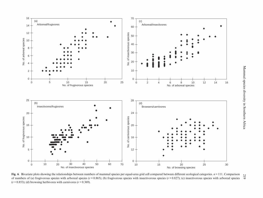
Fig. 6. Bivariate plots showing the relationships between numbers of mammal species per equal-area grid cell compared between different ecological categories. n = 111. Comparison

of numbers of (a) frugivorous species with arboreal species (r = 0.865); (b) frugivorous species with insectivorous species (r = 0.827); (c) insectivorous species with arboreal species

(r = 0.853); (d) browsing herbivores with carnivores (r = 0.369).


15° 20° 25° 30° 35°

15° 20° 25° 30° 35°

15°

20°

25°

30°

35°

15°

20°

25°

30°

35°

(c)

Weight 1–10 kg

50

70

6050

40

40

3010

20

0 500km

15° 20° 25° 30° 35°

15° 20° 25° 30° 35°

15°

20°

25°

30°

35°

15°

20°

25°

30°

35°

(f)

Weight >90 kg

50

70

60

403020

0 500km

70

7075

15° 20° 25° 30° 35°

15° 20° 25° 30° 35°

15°

20°

25°

30°

35°

15°

20°

25°

30°

35°

(b)

Weight 100–1000 g

4030

20

0 500km

30

25

25

25

15

15° 20° 25° 30° 35°

15° 20° 25° 30° 35°

15°

20°

25°

30°

35°

15°

20°

25°

30°

35°

(a)

40

3020

0 500km

2515

3520

Weight 0–100 g15° 20° 25° 30° 35°

15° 20° 25° 30° 35°

15°

20°

25°

30°

35°

15°

20°

25°

30°

35°

(d)

4030

0 500km

20

Weight 10–45 kg

4060

60

7050

80

15° 20° 25° 30° 35°

15° 20° 25° 30° 35°

15°

20°

25°

30°

35°

15°

20°

25°

30°

35°

(e)

40

30

0 500km

Weight 45–90 kg

60

70

50

7070

70

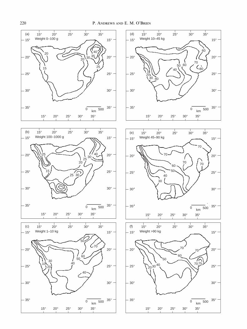
and arboreal species are slightly bigger but almost neverlarge, and carnivorous and omnivorous species areintermediate in size, never small or large. Arising fromthis, we have investigated body size distributions in thestudy area in some detail (Tables 8 & 9) to see if any onepart of the fauna is more strongly linked with vegetationor climate or even with different attributes of thesefactors. Distributions of species richness for the speciesin various size categories are shown in Fig. 7. Theseshould be compared with the distributions of speciesrichness for all mammals and plants in Fig. 3.

The smallest mammals have a distribution thatclosely matches the overall distribution of mammals,with the maximum richness in the north-east of thestudy area, south of the Zambezi river in Mozambiqueand Zimbabwe in the Zambezian mixed woodlands andevergreen forest. This is shown here for mammals< 100 g body weights, size class A (Fig. 7a). Diversityremains high down the eastern highlands and south-eastcoast and decreases westwards to lowest values along

the Namibian coastal desert. The small mammals in sizeclass B, 100±1000 g body weight, have a rather differentdistribution (Fig. 7b). They are only weakly correlatedwith vegetation (Table 8), with plant species richnessaccounting for only 27% of the variability of the speciesin this size class, and when bats are excluded from theanalysis there is no correlation at all. They have adiversity peak in the north-east of the study area, butthey have a secondary peak in the Vaal River basin anda marked decline in diversity south of the Orange Riverin the extension of the Karoo-Namib region into theinterior plateau of western South Africa. In this area,category B mammals decline to only six to seven speciesper grid cell from a maximum of 20 species in the areasof highest diversity. Neither the secondary diversitypeak in the Vaal River region nor the low diversity inthe interior plateau are seen in any other size group,although the latter is present in the distribution offrugivorous species (Fig. 5b). In both this case and withrespect to the frugivorous distribution, this low diversityis the result of the near absence of frugivorous bats, andwhen the maps are generated excluding bats, this lowdiversity phenomenon disappears. On the other hand,the diversity peak in the Vaal River region is even moremarked when bats are excluded.

Large mammal distribution is different from that ofthe small mammals (Fig. 7e, f ). The three largest sizeclasses have been combined in this map since speciesnumbers are low; n = 19 for all mammals > 90kg. Themain trend in the distribution of large mammals is fromsouth to north, with the percentage species richness pergrid cell increasing northwards to high values in northernBotswana and into the Okavango region. There is also apeak in southern Mozambique, as for the smallmammals and mammals generally, and the Namibiancoast has the lowest diversity of large mammals. Thelongitudinal trend that dominates the mammalian rich-ness patterns generally, and the small mammal trends inparticular, are interrupted by this latitudinal trend inthe large mammals. This can be related to the observa-tion from Table 5 that mammal species richness is morestrongly correlated with minimum monthly temperature(TMIN) than with annual temperature (TAN). Lookingat this in more detail (Table 6), it may be seen that thehighest correlations between mammal groups andTMIN are for terrestrial species (r = 0.750) and the sizegroups E (45±90 kg, r = 0.818), F (90±180 kg, r = 0.735)and G (180±360 kg, r = 0.715). At a slightly lower levelthese same groups are also correlated with annualtemperature (TAN, Table 5).

The highest correlation of annual temperature withany mammal group is with size class E, 45±90 kg bodyweight (Table 6, r = 0.77). This size class also has thehighest correlation with minimum monthly temperature


Fig. 7. Isocline maps of distributions of percentage mammal species richness categorized by body weight classes. Species richness

distribution for (a) small mammals 1±100 g (class A); (b) small mammals 100±1000 g (class B); (c) medium-sized mammals,

1±10 kg (class C); (d) medium-sized mammals, 10±45 kg (class D); (e) medium to large mammals, 45±90 kg (class E); (f ) large

mammals, > 90 kg (classes F, G, H). Species numbers are converted into percentages of the total number of species in southern

Africa (n = 285).

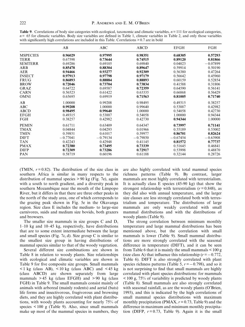
Table 8. Analysis of variance between plant richness andmammal richness by different size categories. Abbreviations asin Table 1. n = 111; P < 0.0001, unless otherwise noted:**P < 0.001; *P < 0.01; NS = not signi®cant, P > 0.01

Plant richness

Size Species Genus Family

A 0±100 g 0.747 0.768 0.639AX Same excluding bats 0.596 0.611 0.681B 100±1000 g 0.272 0.303 0.233BX Same excluding bats NS NS NSC 1±10 kg 0.669 0.679 0.592D 10±45 kg 0.589 0.595 0.587E 45±90 kg 0.262 0.265 0.155F 90±180 kg 0.084* 0.081* NSG 180±360 kg NS NS NSH > 360 kg 0.171 0.175 0.089*

AB 0±1 kg 0.718 0.745 0.615ABX Same excluding bats 0.481 0.505 0.557BC 100 g±10 kg 0.600 0.628 0.525BCX Same excluding bats 0.484 0.506 0.447CD 11±45 kg 0.728 0.739 0.674DE 10±90 kg 0.548 0.554 0.449EF 45±180 kg 0.257 0.258 0.128GH > 180 kg 0.125 0.123** NS

ABC 0±10 kg 0.755 0.781 0.651ABCX Same excluding bats 0.644 0.666 0.667CDE 1±90 kg 0.673 0.682 0.574DEF 10±180 kg 0.532 0.537 0.403EFG 45±360 kg 0.188 0.186 0.063*FGH > 90 kg 0.128 0.126 NS

ABCD 0±45 kg 0.781 0.806 0.684ABCD Excluding bats 0.700 0.721 0.719EFGH > 45 kg 0.211 0.211 0.079*

(TMIN, r = 0.82). The distribution of the size class insouthern Africa is similar in many respects to thedistribution of mammal species > 90 kg (Fig. 7e), againwith a south to north gradient, and a diversity peak insouthern Mozambique near the mouth of the LimpopoRiver, but it differs in that there are three other peaks inthe north of the study area, one of which corresponds tothe grazing peak shown in Fig. 5e in the Okavangaregion. Size class E includes the medium- to large-sizecarnivores, suids and medium size bovids, both grazersand browsers.

The smaller size mammals in size groups C and D,1±10 kg and 10±45 kg, respectively, have distributionsthat are to some extent intermediate between the largeand small species (Fig. 7c, d). Size group C is similar tothe smallest size group in having distributions ofmammal species similar to that of the woody vegetation.

Several different size combinations are shown inTable 8 in relation to woody plants. Size relationshipswith ecological and climatic variables are shown inTable 9 for ®ve composite size groups. Small mammals< 1 kg (class AB), < 10 kg (class ABC) and < 45 kg(class ABCD) are shown separately from largemammals > 45 kg (class EFGH) and > 90 kg (classFGH) in Table 9. The small mammals consist mainly ofanimals with arboreal (mainly rodents) and aerial (bats)life forms and insectivorous, frugivorous and browsingdiets, and they are highly correlated with plant distribu-tions, with woody plants accounting for nearly 75% ofspecies < 100 g (Table 9). Also, since small mammalsmake up most of the mammal species in numbers, they

are also highly correlated with total mammal speciesrichness patterns (Table 9). By contrast, largermammals are most highly correlated with terrestrialism.It is actually class E species (45-90 kg) that show thestrongest relationship with terrestrialism (r = 0.848), asthey did also with annual temperature, and the largersize classes are less strongly correlated both with terres-trialism and temperature. The distributions of largemammals are only weakly correlated with smallmammal distributions and with the distributions ofwoody plants (Table 9).

The strong correlation between minimum monthlytemperature and large mammal distributions has beenmentioned above, but the correlation with smallmammals is lower (Table 9). Small mammal distribu-tions are more strongly correlated with the seasonaldifference in temperature (DIFT), and it can be seenfrom Table 6 that it is mainly the small mammals < 100 g(size class A) that in¯uence this relationship (r =70.772,Table 6). DIFT is also strongly correlated with plantspecies richness patterns (Table 5, r =70.798), and so itis not surprising to ®nd that small mammals are highlycorrelated with plant species distributions: for mammals< 100 g, 75% of variability is predicted by woody plants(Table 8). Small mammals are also strongly correlatedwith seasonal rainfall, as are the woody plants (O'Brien,1993), and this is indicated by the high correlations ofsmall mammal species distributions with maximummonthly precipitation (PMAX, r = 0.73, Table 9) and thedifference in maximum and minimum monthly precipita-tion (DIFP, r = 0.73, Table 9). Again it is the small


Table 9. Correlations of body size categories with ecological, taxonomic and climatic variables, n = 111 for ecological categories,n = 65 for climatic variables. Body size variables are de®ned in Table 1, climate variables in Table 2, and only those variableswith signi®cantly high correlations are included in this Table. Correlations > 0.7 are in bold

AB ABC ABCD EFGH FGH

MSPECIES 0.96029 0.97995 0.98351 0.68305 0.57293TERR 0.67598 0.73644 0.74515 0.89120 0.81866SEMTERR 0.69286 0.69105 0.69840 0.04023 70.07899ARB 0.85478 0.88304 0.89647 0.59914 0.50190AER 0.94466 0.93277 0.92309 0.56380 0.47264INSECT 0.97913 0.97798 0.97179 0.56642 0.45960FRUG 0.86893 0.88884 0.88893 0.60159 0.52854BROW 0.72046 0.73704 0.73834 0.41588 0.31806GRAZ 0.64722 0.69587 0.72359 0.64590 0.56141CARN 0.56523 0.61422 0.63335 0.66868 0.56429OMNI 0.65695 0.69919 0.71563 0.81005 0.71740

AB 1.00000 0.99208 0.98495 0.49315 0.38257ABC 0.99208 1.00000 0.99640 0.53887 0.42982ABCD 0.98495 0.99640 1.00000 0.54058 0.42730EFGH 0.49315 0.53887 0.54058 1.00000 0.94344FGH 0.38257 0.42982 0.42730 0.94344 1.00000

PEMIN 0.61711 0.63409 0.64347 0.73997 0.71141TMAX 0.04844 0.04293 0.01966 0.55189 0.53002TMIN 0.59851 0.61017 0.59977 0.86701 0.82624DIFT 70.77041 70.79134 70.79850 70.67454 70.63908TAN 0.42243 0.42948 0.41145 0.81572 0.77737PMAX 0.72380 0.73495 0.73339 0.51645 0.46841DIFP 0.72309 0.73286 0.72917 0.53998 0.48870PAN 0.58719 0.60196 0.61188 0.32144 0.28726

mammals < 100 g that are most strongly correlated(class A, Table 6).

In summary, small mammal species consisting mainlyof non-terrestrial herbivores have distributions that aremost highly correlated with plant species distributions,seasonality in temperature and precipitation, andmaximum monthly rainfall. Large mammals consistingmainly of terrestrial species have distributions mosthighly correlated with minimum monthly temperatureand annual temperature. They are only weakly corre-lated with regional variations in plant species richnessand the correlates of this.

Model development

The variables that account for most of the variation inmammal species richness based on one-variable, two-variable and three-variable models are examined here bymultiple regression. This analysis is based on the sampleof 65 grid cells that have climate station data. Correla-tion of mammal species richness with that of plants,automatically incorporates the climatic/terrain variablesrelated to plant species richness described earlier,namely annual rainfall, minimum monthly potentialevapotranspiration and topography. As we excludecombinations of variables having similar environmentalfunction, these climatic variables cannot be included ina multiple regression model of mammal richness unlessit does not include vegetation.

For the climate data (n = 65), the best one-variablemodel for mammal species richness is thermal season-ality (DIFT), accounting for 68.9% of mammal speciesrichness (63.1% excluding bats); 69.8% of mammalgenus richness, and 53.9% of mammal family richness(Table 10). The next best models are considerably lesspowerful and include the variables maximum monthlyrainfall (PMAX) and woody plant richness (PGENUSand PSPECIES), which together account for 52.4±54.7%of the variation. In terms of simplicity, i.e. the least

number of variables, the best climate model is PMAXbecause DIFT (and DIFP) are derived from combina-tions of other climatic variables. Vegetation alone, ateither species or genus level, accounts for the sameamount of variation as PMAX, which is consistent withthe strong relationship between vegetation and rainfall(Table 3).

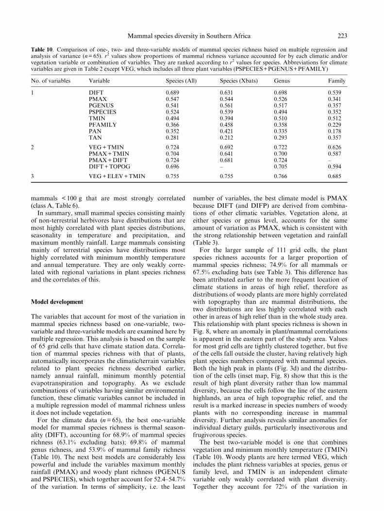
For the larger sample of 111 grid cells, the plantspecies richness accounts for a larger proportion ofmammal species richness; 74.9% for all mammals or67.5% excluding bats (see Table 3). This difference hasbeen attributed earlier to the more frequent location ofclimate stations in areas of high relief, therefore asdistributions of woody plants are more highly correlatedwith topography than are mammal distributions, thetwo distributions are less highly correlated with eachother in areas of high relief than in the whole study area.This relationship with plant species richness is shown inFig. 8, where an anomaly in plant/mammal correlationsis apparent in the eastern part of the study area. Valuesfor most grid cells are tightly clustered together, but ®veof the cells fall outside the cluster, having relatively highplant species numbers compared with mammal species.Both the high peak in plants (Fig. 3d) and the distribu-tion of the cells (inset map, Fig. 8) show that this is theresult of high plant diversity rather than low mammaldiversity, because the cells follow the line of the easternhighlands, an area of high topographic relief, and theresult is a marked increase in species numbers of woodyplants with no corresponding increase in mammaldiversity. Further analysis reveals similar anomalies forindividual dietary guilds, particularly insectivorous andfrugivorous species.

The best two-variable model is one that combinesvegetation and minimum monthly temperature (TMIN)(Table 10). Woody plants are here termed VEG, whichincludes the plant richness variables at species, genus orfamily level, and TMIN is an independent climatevariable only weakly correlated with plant diversity.Together they account for 72% of the variation in


Table 10. Comparison of one-, two- and three-variable models of mammal species richness based on multiple regression andanalysis of variance (n = 65). r2 values show proportions of mammal richness variance accounted for by each climatic and/orvegetation variable or combination of variables. They are ranked according to r2 values for species. Abbreviations for climatevariables are given in Table 2 except VEG, which includes all three plant variables (PSPECIES+PGENUS+PFAMILY)

No. of variables Variable Species (All) Species (Xbats) Genus Family

1 DIFT 0.689 0.631 0.698 0.539PMAX 0.547 0.544 0.526 0.341PGENUS 0.541 0.561 0.517 0.357PSPECIES 0.524 0.539 0.494 0.352TMIN 0.494 0.394 0.510 0.512PFAMILY 0.366 0.458 0.358 0.229PAN 0.352 0.421 0.335 0.178TAN 0.281 0.212 0.293 0.357

2 VEG + TMIN 0.724 0.692 0.722 0.626PMAX + TMIN 0.704 0.641 0.700 0.587PMAX + DIFT 0.724 0.681 0.724 ±DIFT + TOPOG 0.696 ± 0.705 0.594

3 VEG + ELEV + TMIN 0.755 0.755 0.766 0.685

mammal species richness (66.5±71.8% excluding bats).The next best models involve only climate variables, forany relations between VEG and mammal richness auto-matically include the climatic/terrain variables related toplant species richness. Maximum monthly precipitation(PMAX) and TMIN account for 70% variation, andPMAX and thermal seasonality (DIFT) account for72% (Table 10).

There is only one best three-variable model that meetsall criteria: VEG, ELEV and TMIN. These account for75% of the variation in mammal species richness. Thethree next-best models involve only climate variables orterrain, and none are simpler or more parsimoniousthan the two-variable vegetation±climate model. Astriking variation of the three±variable multiple regres-sion was observed when it was run on mammal faunasexcluding bats. In this analysis, the top 20 solutions hadplant family as the sole representative of vegetation,whereas all taxonomic levels were represented for theall-mammal regressions. This is taken to indicate thatthe exclusion of bats resulted in a more generalized andless species-speci®c relationship between mammals andplants.

Annual temperature does not feature as a signi®cantvariable in any of the models, accounting for only 28%of mammal species variation (Tables 5 & 10). Inaddition, it was seen earlier that almost all of that 28%is based on the large mammal element of the mamma-lian fauna, with small mammals being only weaklycorrelated with annual temperature (Table 9). With thisone exception regarding the large mammals, annualtemperature is not a major factor affecting mammalspecies richness in southern Africa.

DISCUSSION

Most animal and plant taxa show predictable diversitygradients, and these have been interpreted as either ofphysico-chemical factors, such as latitude or tempera-ture and their effects on habitat productivity, or as aresult of biological interactions such as competition orpredation (MacArthur, 1965; Thiery, 1982; Begon et al.,1990). It is our contention that climate, particularlyprecipitation and energy, account for most of the ob-served patterns of species richness observed today. Thishas been demonstrated previously for woody plantspecies richness (O'Brien, 1993, 1998), which in turnaccounts for most of the variation in mammal speciesrichness together with other climate variables.

We have found that in the tropical to temperateenvironments of southern Africa, variations in woodyplant richness account for 70±77% of the present-dayvariation in mammal species and genus richness(r2 values, n = 111). Such a close relationship has pre-viously been shown between amphibian species richnessand that of tree species richness in North America(Currie, 1991), but in the same study it was concludedthat mammal diversity was not functionally related totree diversity. Currie (1991) suggests that separateanalysis of different mammal guilds might shed somelight on this issue, and our results show that this is indeedthe case. The weak relationship between plants andmammals that Currie found arises because some parts ofthe mammal fauna are only poorly correlated withwoody plant richness. Large mammals over 90 kg, forexample, and scansorial, aquatic and fossorial mammalsare not signi®cantly correlated with woody plant species


160

140

120

100

80

60

400 100 200 300 400 500 600

Woody plant species richness

Mam

mal

spe

cies

ric

hnes

s

Fig. 8. Bivariate plot showing the relationship between numbers of mammal species per grid cell (n = 285) compared with

numbers of woody plant species (n = 1353; r = 0.865). Inset, outline map of the study area showing the grid cells where plant

diversity is anomalously high.

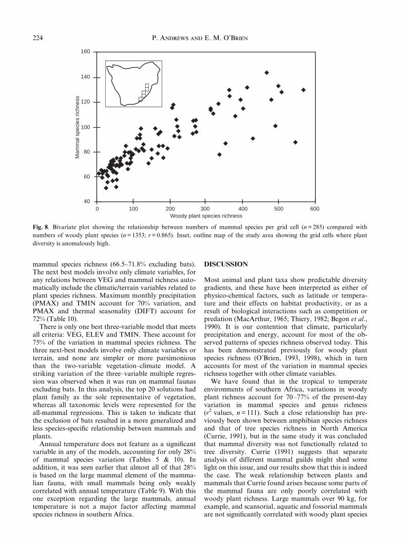
richness (Tables 8 & 9), whereas small-bodied arborealfrugivores and insectivores are strongly correlated(Tables 8 & 9). The pattern of variation in species rich-ness in the former groups of mammal show little changein response to environmental change: e.g. terrestrial (Fig.10a) and carnivorous (Fig. 10c) species show little changein a series of west to east transects across the study area,whereas small-bodied arboreal frugivores and insecti-vores tend to mimic the vegetation pattern (Figs 9 &10b), changing in accord with changes in woody plantrichness. This in turn is related to vegetation structure,being least in desert and greatest in evergreen rainforest,in agreement with results from North America (Fleming,1973; Kerr & Packer, 1997; Fraser, 1998).

It has been observed previously that numbers of largeand small species are not inter-related (Maiorana,1990). There is a general relation between body size andpopulation density, which decreases with body size(Martin, 1990). Energetic requirements are also relatedto trophic level, with basal metabolic rates lower infrugivorous or browsing herbivores (McNab, 1990) andin arboreal mammals as a result of less muscle mass(Grand, 1990), thus reducing population metabolicrequirement. This may be one of the mechanisms per-mitting greater species richness in habitats where thereis an abundant supply of fruit and browse for feedingand trees for space utilization. It is interesting in thisrespect that grazing herbivores have considerably higher


(a) South–north transect

ABCFGH

100

90

80

70

60

50

40

30

20

10

0ff3 ff4 ff5 ff6 ff7 ff8 ff9 ff10 ff11 ff12 ff13

(b) West–east transect

ABCFGH

100

90

80

70

60

50

40

30

20

10

01 2 3 4 5 6 7 8 9 10 11 12 13 14 15

Grid cells

No.

of s

peci

es

Fig. 9. Transect of the study area comparing small mammal variation with large mammal by numbers of species per grid cell

(a) from south to north along 308E longitude; (b) from the west coast along 208S latitude. ABC = small mammals < 10 kg,

n = 230; FGH = large mammals > 90 kg, n = 19.

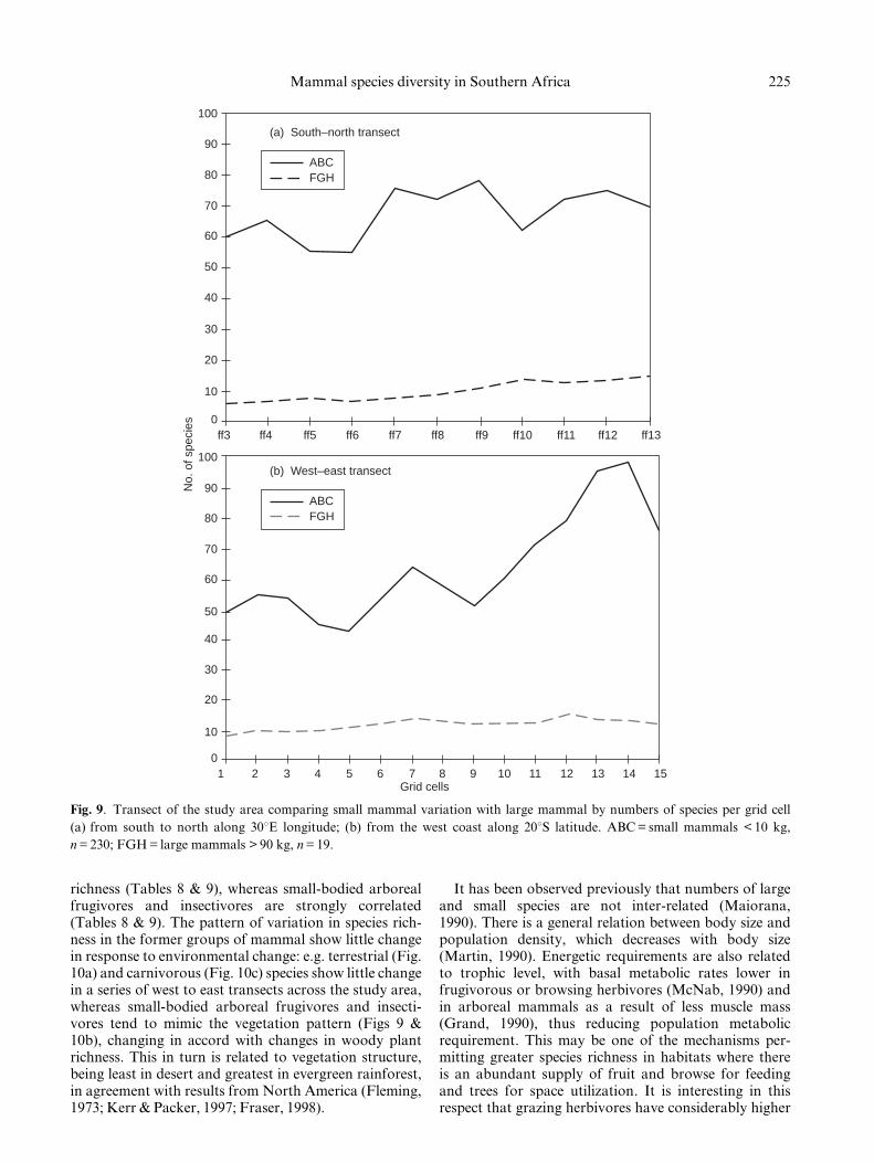
basal metabolic rates (McNab, 1990) than browsers,and this may in part be why we have found that grazersare more highly correlated with woody plant speciesrichness than browsers (Table 7). This is also a result ofthe greater mixture of habitats occupied by grazers as,with one or two exceptions, open grasslands in tropical

Africa are local edaphic phenomena such as ¯ood plainsor dambos, which are associated with forest and wood-land. Grazers are also more highly correlated with mostaspects of climate, particularly the energy, productivityand water variables (Table 6). They are not signi®cantlycorrelated with annual temperature (TAN) in contrastto the signi®cant correlations of large mammals withTAN.

Geographic variations in climate are independent oflife, but they control the capacity for biological activity:the amount and duration of primary productivity, andthus the type, distribution, amount and duration offood resources for consumers. Annual precipitation(PAN) or maximum monthly rainfall (PMAX) are thewater variables most strongly related to woody plantspecies richness; and minimum monthly PET is the moststrongly related energy variable; and together theyaccount for 79% of the predictable pattern of geo-graphic variation in plant taxonomic richness insouthern Africa (O'Brien, 1993). Since slightly over 74%of mammal diversity in turn is predictable from plantdiversity, this degree of variation in mammal richness istherefore an indirect function of climate.

Climate varies geographically, so that as areaincreases the amount of climatic and hence habitatvariability can increase, the extinction rate of bothanimal and plant species may decrease (because largerareas can have a greater range of habitats), and specia-tion rate may increase (more likely to be barriers givingrise to allopatric speciation). Over time these twofactors may lead to an increase in numbers of species,particularly small mammals because their restrictedhabitat range, shorter generation times and higherpotential rates of evolution (Mayr, 1963) may lead tohigher speciation (Van Valen, 1975) and lower extinc-tion rates (Van Valen, 1973). This is probably a majorfactor in the dominance of small mammal speciesnumbers globally, but it is not a suf®cient explanationof why there are particular numbers in speci®c habitatsor areas (May, 1976, 1978). In our analysis we havetaken account of this issue by using an equal-area grid.

As with plants, both the energy and water regimesalso need to be considered when describing the relationof climate to variations in mammal species richness.This is apparent both from the strong correlationbetween mammal and plant species richness andbetween mammal distributions and climatic parameters.In his study of North American animal species richness,Currie (1991) found that annual PET is positivelycorrelated with increases in animal species richness, andhe found this parameter to be the best predictor ofspecies richness of all vertebrate classes. We have found,however, that for mammals in southern Africa it is onlythe large mammals > 45 kg that are signi®cantly corre-lated with annual PET (Table 6). Small mammals arenot signi®cantly correlated with annual PET. In ouranalysis it is minimum monthly PET that is more highlycorrelated with mammal distributions in all categories(Tables 5 & 7). It is also strongly correlated withmeasures of thermal seasonality such as the minimum


No.

of s

peci

es

70

60

50

40

30

20

10

01 2 3 4 5 6 7 8 9 10 11 12 13 14 15

Row 8Row 9Row 10Row 11Row 12Row 13

(a)

16

14

12

10

8

6

4

01 2 3 4 5 6 7 8 9 10 11 12 13 14 15

(b)


2

25

20

15

10

5

01 2 3 4 5 6 7 8 9 10 11 12 13 14

(c)


Grid cells from west to east

Fig. 10. Transects from the west coast of the study area to the

east coast showing numbers of species per grid cell. Row

numbers are given in Fig. 2, with the row of grid cells furthest

to the north being row 13, running through northern Namibia,

northern Botswana, Zimbabwe and Mozambique, and the

furthest south row, row 8, runs through southern Namibia,

Botswana and Mozambique and northern South Africa. (a)

Terrestrial species, n = 102; (b) arboreal species, n = 19; (c)

carnivorous species, n = 29.

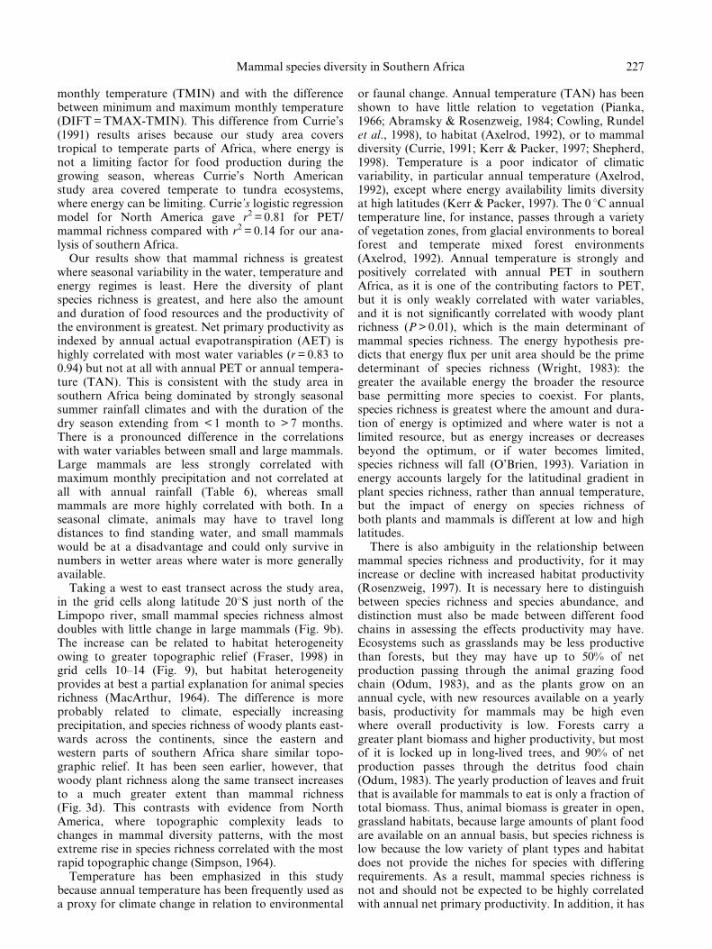
monthly temperature (TMIN) and with the differencebetween minimum and maximum monthly temperature(DIFT = TMAX-TMIN). This difference from Currie's(1991) results arises because our study area coverstropical to temperate parts of Africa, where energy isnot a limiting factor for food production during thegrowing season, whereas Currie's North Americanstudy area covered temperate to tundra ecosystems,where energy can be limiting. Currie's logistic regressionmodel for North America gave r2 = 0.81 for PET/mammal richness compared with r2 = 0.14 for our ana-lysis of southern Africa.

Our results show that mammal richness is greatestwhere seasonal variability in the water, temperature andenergy regimes is least. Here the diversity of plantspecies richness is greatest, and here also the amountand duration of food resources and the productivity ofthe environment is greatest. Net primary productivity asindexed by annual actual evapotranspiration (AET) ishighly correlated with most water variables (r = 0.83 to0.94) but not at all with annual PET or annual tempera-ture (TAN). This is consistent with the study area insouthern Africa being dominated by strongly seasonalsummer rainfall climates and with the duration of thedry season extending from < 1 month to > 7 months.There is a pronounced difference in the correlationswith water variables between small and large mammals.Large mammals are less strongly correlated withmaximum monthly precipitation and not correlated atall with annual rainfall (Table 6), whereas smallmammals are more highly correlated with both. In aseasonal climate, animals may have to travel longdistances to ®nd standing water, and small mammalswould be at a disadvantage and could only survive innumbers in wetter areas where water is more generallyavailable.

Taking a west to east transect across the study area,in the grid cells along latitude 208S just north of theLimpopo river, small mammal species richness almostdoubles with little change in large mammals (Fig. 9b).The increase can be related to habitat heterogeneityowing to greater topographic relief (Fraser, 1998) ingrid cells 10±14 (Fig. 9), but habitat heterogeneityprovides at best a partial explanation for animal speciesrichness (MacArthur, 1964). The difference is moreprobably related to climate, especially increasingprecipitation, and species richness of woody plants east-wards across the continents, since the eastern andwestern parts of southern Africa share similar topo-graphic relief. It has been seen earlier, however, thatwoody plant richness along the same transect increasesto a much greater extent than mammal richness(Fig. 3d). This contrasts with evidence from NorthAmerica, where topographic complexity leads tochanges in mammal diversity patterns, with the mostextreme rise in species richness correlated with the mostrapid topographic change (Simpson, 1964).

Temperature has been emphasized in this studybecause annual temperature has been frequently used asa proxy for climate change in relation to environmental

or faunal change. Annual temperature (TAN) has beenshown to have little relation to vegetation (Pianka,1966; Abramsky & Rosenzweig, 1984; Cowling, Rundelet al., 1998), to habitat (Axelrod, 1992), or to mammaldiversity (Currie, 1991; Kerr & Packer, 1997; Shepherd,1998). Temperature is a poor indicator of climaticvariability, in particular annual temperature (Axelrod,1992), except where energy availability limits diversityat high latitudes (Kerr & Packer, 1997). The 0 8C annualtemperature line, for instance, passes through a varietyof vegetation zones, from glacial environments to borealforest and temperate mixed forest environments(Axelrod, 1992). Annual temperature is strongly andpositively correlated with annual PET in southernAfrica, as it is one of the contributing factors to PET,but it is only weakly correlated with water variables,and it is not signi®cantly correlated with woody plantrichness (P > 0.01), which is the main determinant ofmammal species richness. The energy hypothesis pre-dicts that energy ¯ux per unit area should be the primedeterminant of species richness (Wright, 1983): thegreater the available energy the broader the resourcebase permitting more species to coexist. For plants,species richness is greatest where the amount and dura-tion of energy is optimized and where water is not alimited resource, but as energy increases or decreasesbeyond the optimum, or if water becomes limited,species richness will fall (O'Brien, 1993). Variation inenergy accounts largely for the latitudinal gradient inplant species richness, rather than annual temperature,but the impact of energy on species richness ofboth plants and mammals is different at low and highlatitudes.

There is also ambiguity in the relationship betweenmammal species richness and productivity, for it mayincrease or decline with increased habitat productivity(Rosenzweig, 1997). It is necessary here to distinguishbetween species richness and species abundance, anddistinction must also be made between different foodchains in assessing the effects productivity may have.Ecosystems such as grasslands may be less productivethan forests, but they may have up to 50% of netproduction passing through the animal grazing foodchain (Odum, 1983), and as the plants grow on anannual cycle, with new resources available on a yearlybasis, productivity for mammals may be high evenwhere overall productivity is low. Forests carry agreater plant biomass and higher productivity, but mostof it is locked up in long-lived trees, and 90% of netproduction passes through the detritus food chain(Odum, 1983). The yearly production of leaves and fruitthat is available for mammals to eat is only a fraction oftotal biomass. Thus, animal biomass is greater in open,grassland habitats, because large amounts of plant foodare available on an annual basis, but species richness islow because the low variety of plant types and habitatdoes not provide the niches for species with differingrequirements. As a result, mammal species richness isnot and should not be expected to be highly correlatedwith annual net primary productivity. In addition, it has


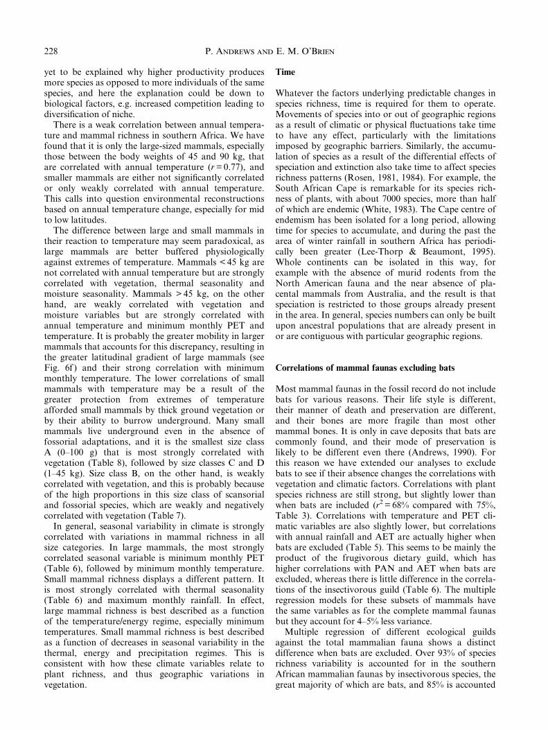
yet to be explained why higher productivity producesmore species as opposed to more individuals of the samespecies, and here the explanation could be down tobiological factors, e.g. increased competition leading todiversi®cation of niche.

There is a weak correlation between annual tempera-ture and mammal richness in southern Africa. We havefound that it is only the large-sized mammals, especiallythose between the body weights of 45 and 90 kg, thatare correlated with annual temperature (r = 0.77), andsmaller mammals are either not signi®cantly correlatedor only weakly correlated with annual temperature.This calls into question environmental reconstructionsbased on annual temperature change, especially for midto low latitudes.

The difference between large and small mammals intheir reaction to temperature may seem paradoxical, aslarge mammals are better buffered physiologicallyagainst extremes of temperature. Mammals < 45 kg arenot correlated with annual temperature but are stronglycorrelated with vegetation, thermal seasonality andmoisture seasonality. Mammals > 45 kg, on the otherhand, are weakly correlated with vegetation andmoisture variables but are strongly correlated withannual temperature and minimum monthly PET andtemperature. It is probably the greater mobility in largermammals that accounts for this discrepancy, resulting inthe greater latitudinal gradient of large mammals (seeFig. 6f ) and their strong correlation with minimummonthly temperature. The lower correlations of smallmammals with temperature may be a result of thegreater protection from extremes of temperatureafforded small mammals by thick ground vegetation orby their ability to burrow underground. Many smallmammals live underground even in the absence offossorial adaptations, and it is the smallest size classA (0±100 g) that is most strongly correlated withvegetation (Table 8), followed by size classes C and D(1±45 kg). Size class B, on the other hand, is weaklycorrelated with vegetation, and this is probably becauseof the high proportions in this size class of scansorialand fossorial species, which are weakly and negativelycorrelated with vegetation (Table 7).

In general, seasonal variability in climate is stronglycorrelated with variations in mammal richness in allsize categories. In large mammals, the most stronglycorrelated seasonal variable is minimum monthly PET(Table 6), followed by minimum monthly temperature.Small mammal richness displays a different pattern. Itis most strongly correlated with thermal seasonality(Table 6) and maximum monthly rainfall. In effect,large mammal richness is best described as a functionof the temperature/energy regime, especially minimumtemperatures. Small mammal richness is best describedas a function of decreases in seasonal variability in thethermal, energy and precipitation regimes. This isconsistent with how these climate variables relate toplant richness, and thus geographic variations invegetation.

Time

Whatever the factors underlying predictable changes inspecies richness, time is required for them to operate.Movements of species into or out of geographic regionsas a result of climatic or physical ¯uctuations take timeto have any effect, particularly with the limitationsimposed by geographic barriers. Similarly, the accumu-lation of species as a result of the differential effects ofspeciation and extinction also take time to affect speciesrichness patterns (Rosen, 1981, 1984). For example, theSouth African Cape is remarkable for its species rich-ness of plants, with about 7000 species, more than halfof which are endemic (White, 1983). The Cape centre ofendemism has been isolated for a long period, allowingtime for species to accumulate, and during the past thearea of winter rainfall in southern Africa has periodi-cally been greater (Lee-Thorp & Beaumont, 1995).Whole continents can be isolated in this way, forexample with the absence of murid rodents from theNorth American fauna and the near absence of pla-cental mammals from Australia, and the result is thatspeciation is restricted to those groups already presentin the area. In general, species numbers can only be builtupon ancestral populations that are already present inor are contiguous with particular geographic regions.

Correlations of mammal faunas excluding bats

Most mammal faunas in the fossil record do not includebats for various reasons. Their life style is different,their manner of death and preservation are different,and their bones are more fragile than most othermammal bones. It is only in cave deposits that bats arecommonly found, and their mode of preservation islikely to be different even there (Andrews, 1990). Forthis reason we have extended our analyses to excludebats to see if their absence changes the correlations withvegetation and climatic factors. Correlations with plantspecies richness are still strong, but slightly lower thanwhen bats are included (r2 = 68% compared with 75%,Table 3). Correlations with temperature and PET cli-matic variables are also slightly lower, but correlationswith annual rainfall and AET are actually higher whenbats are excluded (Table 5). This seems to be mainly theproduct of the frugivorous dietary guild, which hashigher correlations with PAN and AET when bats areexcluded, whereas there is little difference in the correla-tions of the insectivorous guild (Table 6). The multipleregression models for these subsets of mammals havethe same variables as for the complete mammal faunasbut they account for 4±5% less variance.

Multiple regression of different ecological guildsagainst the total mammalian fauna shows a distinctdifference when bats are excluded. Over 93% of speciesrichness variability is accounted for in the southernAfrican mammalian faunas by insectivorous species, thegreat majority of which are bats, and 85% is accounted


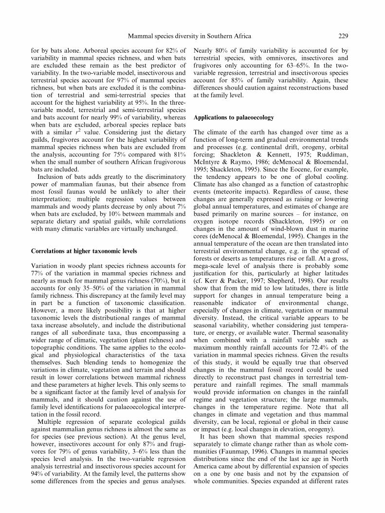
for by bats alone. Arboreal species account for 82% ofvariability in mammal species richness, and when batsare excluded these remain as the best predictor ofvariability. In the two-variable model, insectivorous andterrestrial species account for 97% of mammal speciesrichness, but when bats are excluded it is the combina-tion of terrestrial and semi-terrestrial species thataccount for the highest variability at 95%. In the three-variable model, terrestrial and semi-terrestrial speciesand bats account for nearly 99% of variability, whereaswhen bats are excluded, arboreal species replace batswith a similar r2 value. Considering just the dietaryguilds, frugivores account for the highest variability ofmammal species richness when bats are excluded fromthe analysis, accounting for 75% compared with 81%when the small number of southern African frugivorousbats are included.

Inclusion of bats adds greatly to the discriminatorypower of mammalian faunas, but their absence frommost fossil faunas would be unlikely to alter theirinterpretation; multiple regression values betweenmammals and woody plants decrease by only about 7%when bats are excluded, by 10% between mammals andseparate dietary and spatial guilds, while correlationswith many climatic variables are virtually unchanged.

Correlations at higher taxonomic levels

Variation in woody plant species richness accounts for77% of the variation in mammal species richness andnearly as much for mammal genus richness (70%), but itaccounts for only 35±50% of the variation in mammalfamily richness. This discrepancy at the family level mayin part be a function of taxonomic classi®cation.However, a more likely possibility is that at highertaxonomic levels the distributional ranges of mammaltaxa increase absolutely, and include the distributionalranges of all subordinate taxa, thus encompassing awider range of climatic, vegetation (plant richness) andtopographic conditions. The same applies to the ecolo-gical and physiological characteristics of the taxathemselves. Such blending tends to homogenize thevariations in climate, vegetation and terrain and shouldresult in lower correlations between mammal richnessand these parameters at higher levels. This only seems tobe a signi®cant factor at the family level of analysis formammals, and it should caution against the use offamily level identi®cations for palaeoecological interpre-tation in the fossil record.

Multiple regression of separate ecological guildsagainst mammalian genus richness is almost the same asfor species (see previous section). At the genus level,however, insectivores account for only 87% and frugi-vores for 79% of genus variability, 3±6% less than thespecies level analysis. In the two-variable regressionanalysis terrestrial and insectivorous species account for94% of variability. At the family level, the patterns showsome differences from the species and genus analyses.

Nearly 80% of family variability is accounted for byterrestrial species, with omnivores, insectivores andfrugivores only accounting for 63±65%. In the two-variable regression, terrestrial and insectivorous speciesaccount for 85% of family variability. Again, thesedifferences should caution against reconstructions basedat the family level.

Applications to palaeoecology

The climate of the earth has changed over time as afunction of long-term and gradual environmental trendsand processes (e.g. continental drift, orogeny, orbitalforcing; Shackleton & Kennett, 1975; Ruddiman,McIntyre & Raymo, 1986; deMenocal & Bloemendal,1995; Shackleton, 1995). Since the Eocene, for example,the tendency appears to be one of global cooling.Climate has also changed as a function of catastrophicevents (meteorite impacts). Regardless of cause, thesechanges are generally expressed as raising or loweringglobal annual temperatures, and estimates of change arebased primarily on marine sources ± for instance, onoxygen isotope records (Shackleton, 1995) or onchanges in the amount of wind-blown dust in marinecores (deMenocal & Bloemendal, 1995). Changes in theannual temperature of the ocean are then translated intoterrestrial environmental change, e.g. in the spread offorests or deserts as temperatures rise or fall. At a gross,mega-scale level of analysis there is probably somejusti®cation for this, particularly at higher latitudes(cf. Kerr & Packer, 1997; Shepherd, 1998). Our resultsshow that from the mid to low latitudes, there is littlesupport for changes in annual temperature being areasonable indicator of environmental change,especially of changes in climate, vegetation or mammaldiversity. Instead, the critical variable appears to beseasonal variability, whether considering just tempera-ture, or energy, or available water. Thermal seasonalitywhen combined with a rainfall variable such asmaximum monthly rainfall accounts for 72.4% of thevariation in mammal species richness. Given the resultsof this study, it would be equally true that observedchanges in the mammal fossil record could be useddirectly to reconstruct past changes in terrestrial tem-perature and rainfall regimes. The small mammalswould provide information on changes in the rainfallregime and vegetation structure; the large mammals,changes in the temperature regime. Note that allchanges in climate and vegetation and thus mammaldiversity, can be local, regional or global in their causeor impact (e.g. local changes in elevation, orogeny).

It has been shown that mammal species respondseparately to climate change rather than as whole com-munities (Faunmap, 1996). Changes in mammal speciesdistributions since the end of the last ice age in NorthAmerica came about by differential expansion of specieson a one by one basis and not by the expansion ofwhole communities. Species expanded at different rates


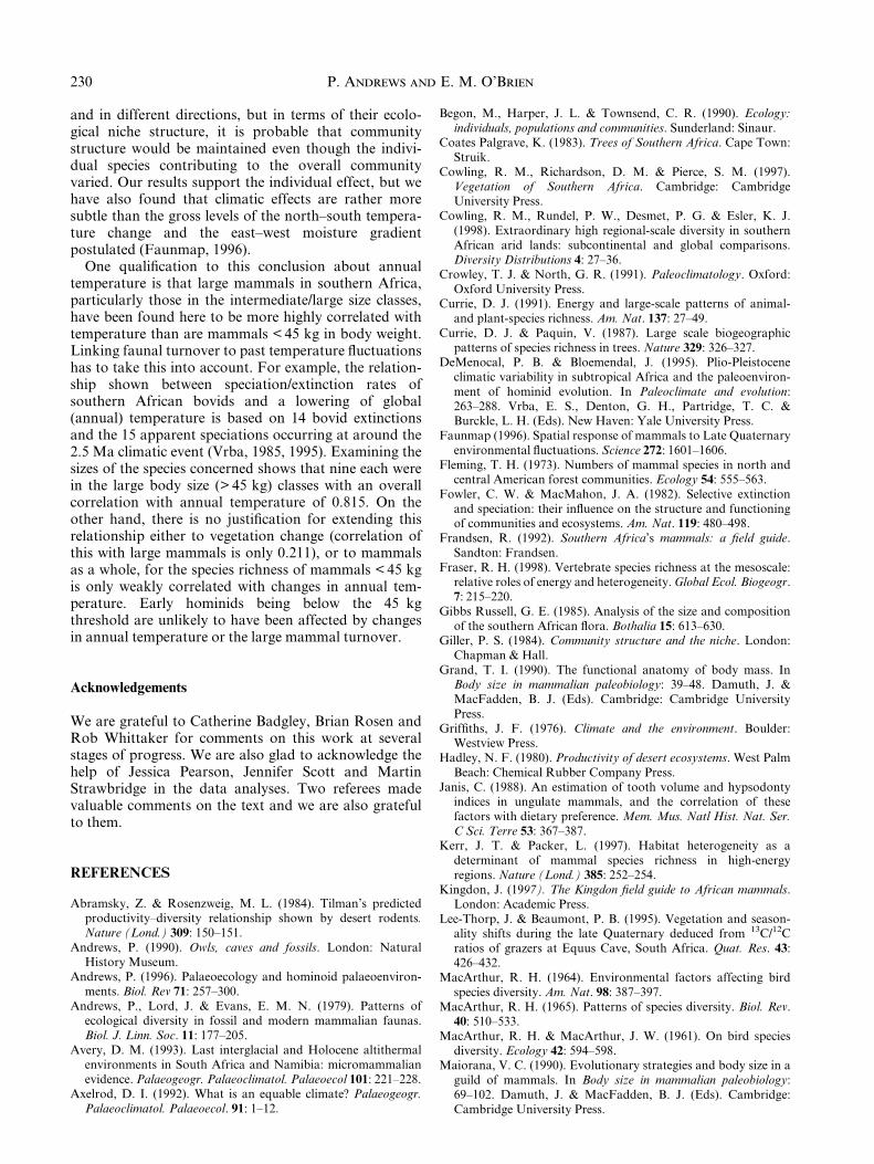
and in different directions, but in terms of their ecolo-gical niche structure, it is probable that communitystructure would be maintained even though the indivi-dual species contributing to the overall communityvaried. Our results support the individual effect, but wehave also found that climatic effects are rather moresubtle than the gross levels of the north±south tempera-ture change and the east±west moisture gradientpostulated (Faunmap, 1996).

One quali®cation to this conclusion about annualtemperature is that large mammals in southern Africa,particularly those in the intermediate/large size classes,have been found here to be more highly correlated withtemperature than are mammals < 45 kg in body weight.Linking faunal turnover to past temperature ¯uctuationshas to take this into account. For example, the relation-ship shown between speciation/extinction rates ofsouthern African bovids and a lowering of global(annual) temperature is based on 14 bovid extinctionsand the 15 apparent speciations occurring at around the2.5 Ma climatic event (Vrba, 1985, 1995). Examining thesizes of the species concerned shows that nine each werein the large body size (> 45 kg) classes with an overallcorrelation with annual temperature of 0.815. On theother hand, there is no justi®cation for extending thisrelationship either to vegetation change (correlation ofthis with large mammals is only 0.211), or to mammalsas a whole, for the species richness of mammals < 45 kgis only weakly correlated with changes in annual tem-perature. Early hominids being below the 45 kgthreshold are unlikely to have been affected by changesin annual temperature or the large mammal turnover.

Acknowledgements

We are grateful to Catherine Badgley, Brian Rosen andRob Whittaker for comments on this work at severalstages of progress. We are also glad to acknowledge thehelp of Jessica Pearson, Jennifer Scott and MartinStrawbridge in the data analyses. Two referees madevaluable comments on the text and we are also gratefulto them.

REFERENCES

Abramsky, Z. & Rosenzweig, M. L. (1984). Tilman's predictedproductivity±diversity relationship shown by desert rodents.Nature (Lond.) 309: 150±151.

Andrews, P. (1990). Owls, caves and fossils. London: NaturalHistory Museum.

Andrews, P. (1996). Palaeoecology and hominoid palaeoenviron-ments. Biol. Rev 71: 257±300.

Andrews, P., Lord, J. & Evans, E. M. N. (1979). Patterns ofecological diversity in fossil and modern mammalian faunas.Biol. J. Linn. Soc. 11: 177±205.

Avery, D. M. (1993). Last interglacial and Holocene altithermalenvironments in South Africa and Namibia: micromammalianevidence. Palaeogeogr. Palaeoclimatol. Palaeoecol 101: 221±228.

Axelrod, D. I. (1992). What is an equable climate? Palaeogeogr.Palaeoclimatol. Palaeoecol. 91: 1±12.

Begon, M., Harper, J. L. & Townsend, C. R. (1990). Ecology:individuals, populations and communities. Sunderland: Sinaur.

Coates Palgrave, K. (1983). Trees of Southern Africa. Cape Town:Struik.

Cowling, R. M., Richardson, D. M. & Pierce, S. M. (1997).Vegetation of Southern Africa. Cambridge: CambridgeUniversity Press.

Cowling, R. M., Rundel, P. W., Desmet, P. G. & Esler, K. J.(1998). Extraordinary high regional-scale diversity in southernAfrican arid lands: subcontinental and global comparisons.Diversity Distributions 4: 27±36.

Crowley, T. J. & North, G. R. (1991). Paleoclimatology. Oxford:Oxford University Press.

Currie, D. J. (1991). Energy and large-scale patterns of animal-and plant-species richness. Am. Nat. 137: 27±49.

Currie, D. J. & Paquin, V. (1987). Large scale biogeographicpatterns of species richness in trees. Nature 329: 326±327.

DeMenocal, P. B. & Bloemendal, J. (1995). Plio-Pleistoceneclimatic variability in subtropical Africa and the paleoenviron-ment of hominid evolution. In Paleoclimate and evolution:263±288. Vrba, E. S., Denton, G. H., Partridge, T. C. &Burckle, L. H. (Eds). New Haven: Yale University Press.

Faunmap (1996). Spatial response of mammals to Late Quaternaryenvironmental ¯uctuations. Science 272: 1601±1606.

Fleming, T. H. (1973). Numbers of mammal species in north andcentral American forest communities. Ecology 54: 555±563.

Fowler, C. W. & MacMahon, J. A. (1982). Selective extinctionand speciation: their in¯uence on the structure and functioningof communities and ecosystems. Am. Nat. 119: 480±498.

Frandsen, R. (1992). Southern Africa's mammals: a ®eld guide.Sandton: Frandsen.

Fraser, R. H. (1998). Vertebrate species richness at the mesoscale:relative roles of energy and heterogeneity. Global Ecol. Biogeogr.7: 215±220.

Gibbs Russell, G. E. (1985). Analysis of the size and compositionof the southern African ¯ora. Bothalia 15: 613±630.

Giller, P. S. (1984). Community structure and the niche. London:Chapman & Hall.

Grand, T. I. (1990). The functional anatomy of body mass. InBody size in mammalian paleobiology: 39±48. Damuth, J. &MacFadden, B. J. (Eds). Cambridge: Cambridge UniversityPress.

Grif®ths, J. F. (1976). Climate and the environment. Boulder:Westview Press.

Hadley, N. F. (1980). Productivity of desert ecosystems. West PalmBeach: Chemical Rubber Company Press.

Janis, C. (1988). An estimation of tooth volume and hypsodontyindices in ungulate mammals, and the correlation of thesefactors with dietary preference. Mem. Mus. Natl Hist. Nat. Ser.C Sci. Terre 53: 367±387.

Kerr, J. T. & Packer, L. (1997). Habitat heterogeneity as adeterminant of mammal species richness in high-energyregions. Nature (Lond.) 385: 252±254.

Kingdon, J. (1997). The Kingdon ®eld guide to African mammals.London: Academic Press.

Lee-Thorp, J. & Beaumont, P. B. (1995). Vegetation and season-ality shifts during the late Quaternary deduced from 13C/12Cratios of grazers at Equus Cave, South Africa. Quat. Res. 43:426±432.

MacArthur, R. H. (1964). Environmental factors affecting birdspecies diversity. Am. Nat. 98: 387±397.

MacArthur, R. H. (1965). Patterns of species diversity. Biol. Rev.40: 510±533.

MacArthur, R. H. & MacArthur, J. W. (1961). On bird speciesdiversity. Ecology 42: 594±598.

Maiorana, V. C. (1990). Evolutionary strategies and body size in aguild of mammals. In Body size in mammalian paleobiology:69±102. Damuth, J. & MacFadden, B. J. (Eds). Cambridge:Cambridge University Press.


Martin, R. A. (1990). Estimating body mass and correlatedvariables in extinct mammals: travels in the fourth dimension.In Body size in mammalian paleobiology: 49±68. Damuth, J. &MacFadden, B. J. (Eds). Cambridge: Cambridge UniversityPress.

May, R. M. (1976). Theoretical ecology. Philadelphia: Saunders.May. R. M. (1978). The dynamics and diversity of insect faunas.

In Diversity of insect faunas: 188±204. Mound, L. A. &Waloff, N. (Eds). Symp. R. Entomol. Soc. No. 9. Oxford:Blackwell.

Mayr, E. (1963). Animal species and evolution. Cambridge:Harvard University Press.

McNab, B. K. (1990). The physiological signi®cance of body size.In Body size in mammalian paleobiology: 11±23. Damuth, J. &MacFadden, B. J. (Eds). Cambridge: Cambridge UniversityPress.

O'Brien, E. M. (1993). Climatic gradients in woody plant speciesrichness: towards an explanation based on an analysis ofsouthern Africa's woody ¯ora. J. Biogeogr. 20: 181±198.

O'Brien, E. M. (1998). Water-energy dynamics, climate andprediction of woody plant species richness: an interim generalmodel. J. Biogeogr. 25: 379±398.

O'Brien, E. M., Whittaker, R. J. & Field, R. (1998). Climate andwoody plant diversity in southern Africa: relationships atspecies genus and family levels. Ecography 21: 495±509.

Odum, E. P. (1983). Basic ecology. New York: Holt Saunders.Pianka, E. R. (1966). Latitudinal gradients in species diversity: a

review of concepts. Am. Nat. 100: 33±46.Rosen, B. R. (1981). The tropical high diversity enigma ± the

corals'-eye view. In Chance, change and challenge. The evolvingbiosphere: 103±129. Forey, P. L. (Ed.). London: British NaturalHistory Museum.

Rosen, B. R. (1984). Reef coral biogeography and climate throughthe late Cainozoic: just islands in the sun or a critical pattern ofislands? Geol. J. spec. Issues 11: 201±262.

Rosenzweig, M. L. (1968). Net primary productivity of terrestrialenvironments: predictions from climatological data. Am. Nat.102: 67±84.

Rosenzweig, M. L. (1997). Species diversity in space and time.Cambridge: Cambridge University Press.

Ruddiman, W. F., McIntyre, A. & Raymo, M. (1986). Matyuama41,000 year cycles North Atlantic Ocean and northern hemi-sphere ice sheets. Earth Planet Sci. Lett. 80: 117±129.

Sanders, H. L. (1968). Marine benthic diversity: a comparativestudy. Am. Nat. 102: 243±282.

Schulz, R. E. & McGee, O. S. (1977). Climatic indices andclassi®cations in relation to the biogeography of southernAfrica. In Biogeography and ecology of Southern Africa: 21±60.Werger, M. J. A. (Ed.). The Hague: W. Junk.

Seely, M. K. & Louw, G. N. (1980). First approximation of theeffects of rainfall on the ecology and energetics of a Namibdesert dune ecosystem. J. Arid Environ. 3: 25±54.

Shackleton, N. (1995). New data on the evolution of Plioceneclimatic variability. In Paleoclimate and evolution: 242±248.Vrba, E. S., Denton, G. H., Partridge, T. C. & Burckle, L. H.(Eds). New Haven: Yale University Press.

Shackleton, N. & Kennett, J. P. (1975). Paleotemperature historyof the Cenozoic and the initiation of Antarctic glaciation:oxygen and carbon isotope analyses in DSDP Sites 277, 279and 281. Initial Rep. Deep Sea Drill Project 29: 743±756.

Shepherd, U. L. (1998). A comparison of species diversity andmorphological diversity across the North American latitudinalgradient. J. Biogeogr. 25: 19±29.

Simpson, G. G. (1964). Species diversity of North Americanrecent mammals. Syst. Zool. 13: 57±73.

Smithers, R. H. N. (1983). The mammals of the Southern Africansubregion. Pretoria: Pretoria University.

Stuart, C. & Stuart, T. (1988). Field guide to the mammals ofSouthern Africa. London: New Holland.

Thiery, R. G. (1982). Environmental instability and communitydiversity. Biol. Rev. 57: 671±710.

Thornthwaite, C. W. & Mather, J. R. (1955). The water balance.Publ. Climatol. No. 8. Centerton, NJ: Laboratory ofClimatology,

Thornthwaite, C. W. & Mather, J. R. (1962). Average climaticwater balance data of the continents. Part I. Africa. Publ.Climatol. No. 15. Centerton, NJ: Laboratory of Climatology.

Tyson, P. D. (1986). Climatic change and variability in southernAfrica. Oxford: Oxford University Press.

Van der Heijden, M. G. A., Klironomos, J. N., Ursic, M.,Moutoglis, P., Streitwolf-Engel, R., Boller, T., Wiemken, A. &Sanders, I. (1998). Mycorrhizal fungal diversity determinesplant biodiversity ecosystem variability and productivity.Nature (Lond.) 396: 69±72.

Van Valen, L. (1973). Body size and numbers of plants andmammals. Evolution 27: 27±35.

Van Valen, L. (1975). Group selection, sex and fossils. Evol.Theory 1: 1±30.

Vrba, E. S. (1985). Environment and evolution: alternative causesof the temporal distribution of evolutionary events. S. Afr. J.Sci. 81: 229±236.

Vrba, E. S. (1995). On the connections between paleoclimate andevolution. In Paleoclimate and evolution: 24±45. Vrba, E. S.,Denton, G. H., Partridge, T. C. & Burckle, L. H. (Eds). NewHaven: Yale University Press.

White, F. (1981). Vegetation map of Africa. Paris: UNESCO/AETFAT/UNESCO.

White, F. (1983). The vegetation of Africa: a descriptive memoir toaccompany the UNESCO/AETFAT/UNSO vegetation map ofAfrica. Paris: UNESCO.

Wilson, E. E. & Reeder, D. M. (1992). Mammal species of theWorld. Washington: Smithsonian Institution Press.

Wright, D. H. (1983). Species±energy theory: an extension ofspecies±area theory. Oikos 41: 496±506.


Documents

Climate, vegetation, and predictable gradients in mammal ...sysecol2.ethz.ch/Refs/EntClim/A/An303.pdf · Climate, vegetation, and predictable gradients in mammal species richness