School of Science and Engineering

Capstone Final Report

Profitability Analysis of Large-Scale Photovoltaic

Power Plants

Written by

Ayoub El Haimar

Supervised by

Dr. Kissani Ilham

Submitted on: 20th April (Spring 2015)

1

Contents ACKNOWLEDGMENT ............................................................................................................................... 3

ABSTRACT .................................................................................................................................................. 4

INTRODUCTION ........................................................................................................................................ 5

1. Motivation: ...................................................................................................................................... 5

2. Challenges: ....................................................................................................................................... 6

3. Objectives: ....................................................................................................................................... 6

4. Overview of the Energy Sector in Morocco: ................................................................................. 6

BACKGROUND .......................................................................................................................................... 8

1. Solar Energy Harnessing Technology: .......................................................................................... 8

2. Mathematical Background: ........................................................................................................... 9

For sections 2.2 till 2.4, most of the mathematical background was found in [6]. ................................... 9

2.1 The Monte Carlo Simulation: .................................................................................................. 9

2.2 The Generalized Lognormal Distribution: ............................................................................ 10

2.3 SimTools: ................................................................................................................................ 11

2.4 Subjective Probability Assessment: ....................................................................................... 12

DESIGN OF THE FINANCIAL MODEL ................................................................................................. 13

1. Overview of the Methodology: ..................................................................................................... 13

2. Estimations and Assumptions: ..................................................................................................... 15

2.1 Fixed Costs and Electricity Selling Price: ............................................................................. 15

2.2 Logarithmic Growth Rate Estimations: ................................................................................ 16

2.3 Expected Plant Production: ................................................................................................... 17

2.4 Subjective Probability Assessment of the 5th Year Sales: .................................................... 18

RESULTS OF THE MONTE CARLO SIMULATION AND DISCUSSION ........................................... 19

1. Simulation of Sales: ....................................................................................................................... 19

2. Cash Flow Model: ......................................................................................................................... 20

3. The Simulation Results for the Profits NPV: ............................................................................. 21

4. Discussion: ..................................................................................................................................... 23

CONCLUSION ........................................................................................................................................... 25

STEEPLE ANALYSIS ............................................................................................................................... 26

1. Social: ............................................................................................................................................. 26

2. Technological: ............................................................................................................................... 26

3

ACKNOWLEDGMENT

First of all, I would like to thank Al Akhawayn University and the School of Science &

Engineering, for providing me with a good environment to work on this project entitled

“Profitability Analysis of Large-Scale Photovoltaic Power Plants”. Also, I am thankful to Dr.

Ilham Kissani for all the efforts and time she allocated to my supervision while working on this

project and for providing me with the necessary knowledge, tools and support I needed. I would

like to express my gratitude to Dr. Ilham Kissani for accepting to be my supervisor and for being

always welcoming and professional. I would like to thank Dr. Yassine Saleh Alj for making the

capstone requirements clear and concise as well as for organizing very interesting talks/lectures.

Last but not least, I would like to express my deepest appreciation to my family and

friends for giving me the moral strength I needed to work on this capstone throughout the whole

semester.

4

ABSTRACT

This report provides a study of the economic viability of investing in utility-scale

photovoltaic power plants that will be used to generate electricity that will be fed into the grid. In

fact, the study will be an application of simulation modeling and uncertainty analysis. The

project will start with a cost-benefit analysis that is intended to estimate the costs related to

building/extending/maintaining the facility as well as the benefits that may be generated through

selling electricity to the local power company. Simulation modeling and uncertainty analysis will

be used to estimate the net present value of profits from the proposed project over a certain

period of time. Two plans are considered; the first consists of continuing the extension of the

plant regardless of the first year’s sales, while the second consists of terminating the project in

case the first year’s sales performance falls below a given threshold. The main technique that

will be used is the Monte Carlo simulation using Simtools in Excel. The results show that

utility-scale Photovoltaic plants are profitable on the long run. Also, the two plans are compared

based on the simulations and the 1st one proves to be best option.

5

INTRODUCTION

Recently, there has been a significantly increasing interest in renewable energies all over

the world. The need to reduce the emission of greenhouse gases, the constantly increasing energy

demand and the shrinking energy resources imply that we should switch to renewable energies as

clean, abundant and cheap forms of energy. In a country like Morocco, where there is a heavy

reliance on imported fossil fuels to satisfy energy demands, switching to green energy is not just

an option; it is a priority. In addition to the very high cost of importing energy, it impedes the

socio-economic development of the country as the heavy reliance on imports makes it difficult to

adjust energy supply to energy demand.

Furthermore, the energy produced by private renewable energy producers is mainly

targeted at industrials. So, investing in solar energy businesses that are targeted at households

supply needs to be considered to reduce the reliance on fossil fuels. Therefore, the profitability of

such an investment has to be able to assess its economic viability.

1. Motivation:

Undoubtedly, Morocco will have a bright future in the field of renewable energies,

especially solar energy. In fact, the country has very important solar resources with a potential of

2600 kWh/m2/year [1]. Such an extremely significant irradiation necessitates that we think about

ways we can fully exploit it. Although Morocco is the only African country that has the most

ambitious solar energy project, the pace at which the sector is growing needs to be boosted.

Actually, the Moroccan solar energy project aims at developing 2000 MW by 2020, and that is a

very promising target. However, since these kinds of projects are very large, they usually require

a lot of time and money. That is why, encouraging investment in small solar energy plants that

6

will generate electricity for home-use can be more appealing to individual investors. However,

the potential of such projects has to be investigated before proceeding with the investment.

Indeed, setting up even a small solar business costs a lot of money and realizing substantial

returns at the beginning will certainly be difficult.

2. Challenges:

The main challenge in this project is the scarcity of data. In fact, since this kind of power

facilities is not very popular yet in Morocco, it is very difficult to come up with good estimates

of costs and benefits within the Moroccan context. In light of this situation, the latter values will

be rounded to the best possible estimates. Moreover, most of the tools and techniques I will use

in this project are ones I encounter for the first time. This requires of course a lot of reading and

practice so that I can apply general concepts to this very specific case.

3. Objectives:

The main goal of this project is to come up with a simulation model that can be used to

estimate the expected net present value of profits from investing in a solar energy business.

Doing so will help us better understand how such investment can be undertaken. Different

investment options will be analyzed in order to see the risks involved in each option. Such an

analysis will help us get some insights into the economic viability of photovoltaic power plants

as a private investment.

4. Overview of the Energy Sector in Morocco:

It is very well known that Morocco is highly dependent on foreign imports (mainly

hydrocarbons) to satisfy its domestic energy needs. According to the World Bank, in 2011 the

7

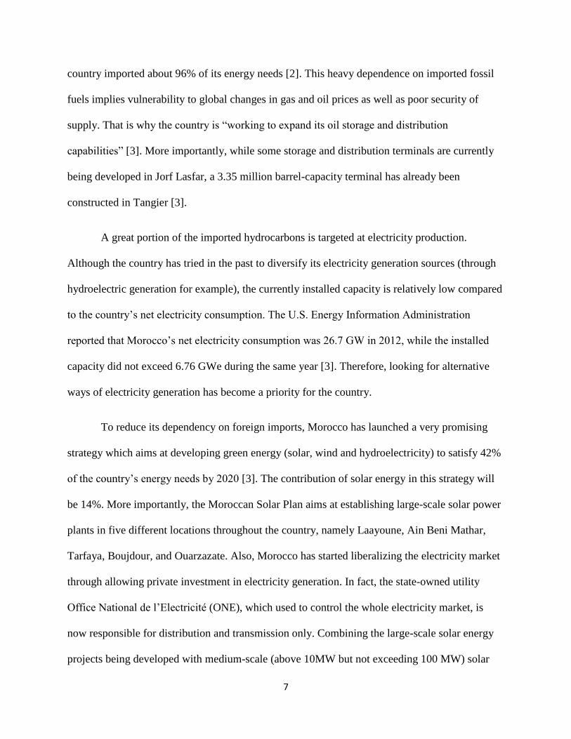
country imported about 96% of its energy needs [2]. This heavy dependence on imported fossil

fuels implies vulnerability to global changes in gas and oil prices as well as poor security of

supply. That is why the country is “working to expand its oil storage and distribution

capabilities” [3]. More importantly, while some storage and distribution terminals are currently

being developed in Jorf Lasfar, a 3.35 million barrel-capacity terminal has already been

constructed in Tangier [3].

A great portion of the imported hydrocarbons is targeted at electricity production.

Although the country has tried in the past to diversify its electricity generation sources (through

hydroelectric generation for example), the currently installed capacity is relatively low compared

to the country’s net electricity consumption. The U.S. Energy Information Administration

reported that Morocco’s net electricity consumption was 26.7 GW in 2012, while the installed

capacity did not exceed 6.76 GWe during the same year [3]. Therefore, looking for alternative

ways of electricity generation has become a priority for the country.

To reduce its dependency on foreign imports, Morocco has launched a very promising

strategy which aims at developing green energy (solar, wind and hydroelectricity) to satisfy 42%

of the country’s energy needs by 2020 [3]. The contribution of solar energy in this strategy will

be 14%. More importantly, the Moroccan Solar Plan aims at establishing large-scale solar power

plants in five different locations throughout the country, namely Laayoune, Ain Beni Mathar,

Tarfaya, Boujdour, and Ouarzazate. Also, Morocco has started liberalizing the electricity market

through allowing private investment in electricity generation. In fact, the state-owned utility

Office National de l’Electricité (ONE), which used to control the whole electricity market, is

now responsible for distribution and transmission only. Combining the large-scale solar energy

projects being developed with medium-scale (above 10MW but not exceeding 100 MW) solar

8

energy plants will certainly help the country exploit more its important renewable energy

resources and further reduce its dependency on energy imports.

BACKGROUND

1. Solar Energy Harnessing Technology:

Indeed, there are many technologies used to harness solar energy, but the one we chose to

consider in this study is solar Photovoltaic (PV) modules. The latter are formed by connecting

many PV cells together. Actually, PV cells convert sunlight into electricity using the

photoelectric effect. PV arrays are the building blocks of solar farms and they consist of many

PV modules connected together. PV modules are not the only component of PV systems.

Additional components of a PV system include electrical connections, batteries (if needed),

equipment used for power conditioning such as inverters, trackers etc… Figure 1.1 shows a PV

array, a PV module and a PV cell.

Figure 1.1: “Depiction of PV system modularity” [4]

9

One may argue that CSP technology could have been a more viable choice within the

Moroccan context. However, in his analysis of the Moroccan Solar Plan, Richts argues that “it is

not very likely that CSP will be less costly than PV” [5]. Also, taking into consideration the

relative technological simplicity of PV systems (compared to CSP systems), it seems more

appealing to go for PV modules.

2. Mathematical Background:

For sections 2.2 till 2.4, most of the mathematical background was found in [6].

2.1 The Monte Carlo Simulation:

The Monte Carlo simulation can be defined as a technique used to generate an

approximation of certain outcomes by performing many simulations using different random

input variables. In fact, this method consists of converting the uncertainty in the input

variables of a model into probability distributions to help reduce the uncertainty and risk

involved in estimating the values of the output variables [7].

As it is the case with most statistical analysis situations, the larger the sample size you

analyze the more accurate will be the conclusions you make. More importantly, within the

context of the Monte Carlo simulation, the more simulations we perform the more accurate

will be the approximation of the outcomes. However, the Monte Carlo simulation does not

ensure there will be no uncertainty or risk involved; it is just a way to predict the future

through running multiple (thousands or even millions) trials that are targeted at analyzing the

probability of certain outcomes.

10

2.2 The Generalized Lognormal Distribution:

Generalized-lognormal distributions is a family of probability distributions that is

characterized by 3 parameters, which are called the quartile boundary points. Actually, the

latter are values that divide the probability region (area under the probability curve) into four

regions which are equally likely to involve the actual value of the unknown variable

described by this kind of distributions. This means that the 3 quartile boundary points, which

we may denote by Q1, Q2 and Q3, correspond to the values of the Generalized-Lognormal

probability distribution at the cumulative probability levels 0.25, 0.5 and 0.75, respectively.

Therefore, the four regions or quartiles delimited by the quartile boundary points all have the

same probability which is ¼.

This family of probability distributions describes random variables of the form c*X + d

such that X is a normal or lognormal random variable. Actually, a random variable Y is said

to be log-normally distributed if its natural logarithm LN(Y) follows a normal distribution.

Therefore, if we take the exponential of any normal random variable with mean μ and

standard deviation σ, we will get a lognormal variable with log-mean μ and log-standard

deviation σ. The normal and lognormal distributions are just special cases of the Generalized-

lognormal probability distribution. The latter becomes a normal distribution when the

quartile boundary points have equal differences; that is, when Q3 – Q2 = Q2 – Q1. In this case,

the mean of the normal random variable is Q2. Since the natural logarithm of a lognormal

random variable follows a normal distribution, a random variable X following a Generalized-

Lognormal distribution turns out to be a lognormal variable when LN(X) is normally

distributed, meaning that:

11

LN(Q3) - LN(Q2) = LN(Q2) - LN(Q1)

Which implies that: LN(Q3/Q2) = LN(Q2/Q1)

Since the natural logarithm is a one-to-one function, the equality above implies that:

Q3/Q2 = Q2/Q1

Hence, we can say that the generalized lognormal distribution turns out to be a lognormal

distribution when the quartile boundary points have equal ratios. In this case, the log-mean of

the lognormal random variable is LN(Q2).

2.3 SimTools:

The statistical tool we will be using in our analysis is SimTools. Actually, SimTools

is an Excel add-in that provides statistical functions and procedures for performing the Monte

Carlo simulation and risk analysis in excel sheets. This add-in adds to Excel different

categories of functions and procedures, among which there is:

Inverse Cumulative Probability Functions

Functions for Working with Correlations among random variables

Functions for decision analysis

Functions for analyzing discrete probability distributions

Functions for regression analysis

Functions for randomly generating discrete distributions

The main category of functions we will be using in our uncertainty analysis is the inverse

cumulative probability functions. Given a cumulative probability level, these functions can

be used to compute the value of a certain random variable corresponding to that specific

12

probability level. For instance, among the functions provided by Simtools there is

NORMINV(), which is the inverse cumulative probability function for normal probability

distributions. This function takes as parameters a cumulative probability level, the mean of a

normal random variable and its standard deviation, and produces as an output the value of the

normal random variable corresponding to the specified cumulative probability level. Also,

among the functions we will be using in our simulation, there is the RAND() function. The

latter is used to generate random numbers between 0 and 1, and thus it can be used to

randomly generate cumulative probability levels. Actually, if we combine an inverse

cumulative probability function such as NORMINV() with the RAND() function; that is, if

we use the result of RAND() as the cumulative probability level instead of providing a

specific number, we can randomly generate values of a given normal random variable.

Similarly, we can use a function called GENLINV() with RAND() to simulate a random

variable that follows the Generalized Lognormal distribution. Also, we can simulate a

lognormal random variable through simulating its natural logarithm (which is a normal

random variable) and then taking the exponential of the simulated result. In other words, if

we have a lognormal random variable with log-mean m and log-standard deviation s, we can

simulate the variable using EXP(NORMINV(RAND(), m, s)).

2.4 Subjective Probability Assessment:

The uncertainty involved in any unknown quantity can be hard to describe by a

probability distribution if there is no comparable data for the random variable we are trying

to model. For instance, if we are taking into consideration a certain stock price for which we

already have historical records of at least the last 30 years, we may use that historical data to

predict the stock price in the future. However, in case we are trying to predict the potential

13

demand for a new product, it will be inappropriate to use the performance of products that

have been introduced in the past in the sense that we would neglect the features and

specificities of the new product.

Indeed, in a lot of situations uncertainty analysis is difficult, but one can still describe the

uncertainty about an unknown quantity using some probability distribution. Actually, anyone

can use the information that is available to them at a specific point in time to come up with a

model that describes his/her beliefs about an unknown quantity. Such an assessment is

subjective in the sense that different people will have different beliefs about a given quantity.

That is why it is called subjective probability assessment. In practice, to subjectively assess

an unknown quantity with continuous distribution, we often start with an assessment of the

three quartile points that divide the area under the curve into four equally likely intervals.

DESIGN OF THE FINANCIAL MODEL

1. Overview of the Methodology:

The economic analysis that will be undertaken in this study consists of assessing the

economic viability of investing in a large-scale PV power plant through simulation of the net

present worth of the profits that may be realized over a period of 15 years. Since the investment

will have a huge capital cost, we will assume that it will staggered by the investor over 5 years

through incrementing the capacity of the facility during the 5 1st years. In fact, we will be

considering two investment plans that may be considered by investors in PV power plants. The

first plan consists of continuing the extension of the facility regardless of the amount of sales

(annual sales will be measured in kWh) made in the first year. As for the second plan, the project

14

will be terminated if we do not reach a certain amount of sales at the end of the first year of

operation. Because comparable data that would provide good costs and benefits estimates of such

plants is scarce, a lot of assumptions need to be made in order to facilitate our analysis.

The economic viability of investing in solar PV plants will be analyzed through simulation of

the Net Present Value (NPV) of the annual cash flows that may be generated from selling the

electricity generated by the plant over a period of 15 years, using a 2.5 % discount rate. The

simulation will be done on Excel. As it is the case with any new product or service, it is really

hard to achieve a good amount of sales at the very beginning. In reality, what happens is that the

sales keep growing significantly during the first years until they reach a level around which they

will keep varying in the future. Therefore, we will be using the annual logarithmic growth rate to

predict the energy sales that may be realized from exploiting a 25 MW solar PV plant. The

assumptions made to estimate the fixed costs, the logarithmic growth rate of sales, and the

benefits will be discussed later in the report.

In the absence of a regulatory framework with respect to which we can develop our financial

model, we will assume that the energy generated can be either sold directly to subscribers or to

the state-owned utility ONE that will take care of the distribution. It can also be a combination of

the two although it is sometimes hard to cover all subscribers’ needs by solar energy solely.

When power is sold to a customer, a Power Purchase Agreement (PPA) is signed between the

power producer and its customer(s). Such an agreement imposes on the power producer to keep

supplying energy at a fixed price throughout the duration of the agreement without taking into

consideration the changes in prices [7]. We will assume that the power supplied to the grid will

not necessarily be the total power produced by the plant. Also, we will assume that the PV power

plant will be built in the region of Ouarzazate.

15

2. Estimations and Assumptions:

All the tables listed below were taken from the Excel sheet that was used for simulation.

2.1 Fixed Costs and Electricity Selling Price:

Before discussing the costs estimation, it is worth mentioning that all costs and benefits

will be expressed in U.S. dollars. The costs that were taken into consideration are the capital cost

(i.e. the construction cost) and the fixed Operations and Maintenance (O&M) cost. According to

Lazard’s Levelized Cost of Energy Analysis, it can be assumed that a utility-scale PV power

plant with single-axis tracking would cost around 1750 $/kW, while the O&M cost of such a

plant would be 20 $/kW-year [8]. So, a rough estimation of a 25MW plant capital cost would be:

25000 kW * 1750 $/kW = $43750000

The investment will be staggered over a period of 5 years, which means that the installation will

be done through 5 stages. During the 1st stage (at the beginning of the 1

st year), the installed

capacity will be 10 MW, and it will be extended by 6 MW in the 2nd

year, then by 5 MW in the

3rd

year, and finally by 2 MW in each of the 4th

and 5th

years so that we reach a final capacity of

25 MW. The selling price of the generated electricity is assumed to be 0.12 $/kWh.

The fixed costs of building/extending/maintaining the PV power plant as well as the electricity

selling price are summarized in table 2.1.1:

Year 1 (10 MW) -$17,500,000

Year 2 (6 MW) -$10,500,000

Year 3 (5 MW) -$8,750,000

Years 4 & 5 (2 MW) -$3,500,000

Variable O&M cost ($/kW-yr) -$20.00

Power price/kWh ($/kWh) $0.12

Table 2.1.1: Fixed Costs and Electricity Selling Price

16

2.2 Logarithmic Growth Rate Estimations:

The annual logarithmic growth rate of electricity sales is assumed to have the statistics

shown in will table 2.2.1.

Year E(ln(St/St-1)) Stdev(ln(St/St-1))

1

2 0.5 0.3

3 0.3 0.2

4 0.2 0.15

5 0.1 0.07

6 0 0.04

7 0 0.04

8 0 0.04

9 0 0.04

10 0 0.04

11 0 0.04

12 0 0.04

13 0 0.04

14 0 0.04

15 0 0.04

Table 2.2.1: The assumed annual logarithmic growth

Table 2.2.1 lists the expected value and standard deviation of the annual sales logarithmic growth

rate for a period of 15 years. For each year t, St represents the sales realized during that year,

while St-1 represents the sales of the previous year. The growth is expected to be high during the

first 5 years because the capacity of the plant will be substantially increased during that period

with annual capacity increments decreasing each year as discussed in section 2.1. In fact, the

logarithmic growth rate can be affected by many factors like meteorological conditions of the

site, the nature of the PPA, the consumption or needs of individual customers (in case we are

supplying power to different customers) etc… To simplify the complexity of reality, let us

assume that the suggested statistics of the sales logarithmic growth rate represent a good

17

estimation of what the growth would really be. To simulate the logarithmic growth rate for each

year, we use the NORM.INV function as the following:

NORM.INV(RAND(), E(ln(St/St-1)), Stdev(ln(St/St-1)))

2.3 Expected Plant Production:

First Solar, which is a leading manufacturer of solar PV modules designed for large-scale

PV plants, provides an Energy Capacity Assessment tool on its website for energy investors.

This tool gives the possibility to calculate the expected plant production of a solar PV plant that

the user can plot on a map. More importantly, this tool can be used to predict the output of a PV

power plant anywhere in the world using that location’s specific irradiation and meteorological

conditions. Table 2.3.1 shows the expected electricity production of the plant over the 15 years

period.

Year Expected Power Production

(kWh)

1 23500000

2 36500000

3 49500000

4 54000000

5 58000000

6 58000000

7 58000000

8 58000000

9 58000000

10 58000000

11 58000000

12 58000000

13 58000000

14 58000000

15 58000000 Table 2.3.1: Expected power production estimated using First Solar’s Energy Capacity

Assessment Tool [9]

18

2.4 Subjective Probability Assessment of the 5th Year Sales:

It was assumed that the sales during the 5th

year follow a generalized-lognormal

probability distribution. Table 2.4.1 shows the subjectively assessed quartile boundary points of

sales in the 5th

year that were obtained based on the recommendations of subject matter experts.

Quartiles Q1 Q2 Q3

Sales in Year 5 (kWh) 55000000 56500000 57500000

Table 2.4.1: Subjectively assessed quartiles boundary points for year 5

These quartile boundary points are used to simulate the sales in the 5th

year. If we check for the

equality of differences (whether Q3-Q2 = Q2-Q1) and equality of ratios (whether Q3/Q2 =

Q2/Q1), we find that neither of them is satisfied. Therefore, the simulation of the 5th

year sales is

done using the Inverse Cumulative Probability function:

GENLINV(RAND(),55000000, 56500000, 57500000)

When the sales in year 5 are simulated, the simulated annual sales growth rates are used to

calculate the simulated sales for the previous years, using the following formula:

St = St+1 / Exp(LGRt+1)

where LGRt+1 denotes the Logarithmic Growth Rate corresponding to the year following the one

we are interested in. Similarly, the simulated annual sales growth rates are used to calculate the

simulated sales for the years following the 5th

year, using the following formula:

St = St-1 * Exp(LGRt)

19

RESULTS OF THE MONTE CARLO SIMULATION AND DISCUSSION

1. Simulation of Sales:

Table 1.1 shows the expected growth and sales corresponding to each of the 15 years.

Year

E(ln(st/st-1))

Stdev(ln(st/st-1)) Growth

Energy Sales (kWh)

Expected Power Production (kWh)

1 14890585.93 23500000

2 0.5 0.3 0.4533697

52 23431914.22 36500000

3 0.3 0.2 0.7478737

21 49500000 49500000

4 0.2 0.15

-0.1205945

5 44168131.8 54000000

5 0.1 0.07 0.1715427

69 52433531.36 58000000

6 0 0.04 0.0029738

38 52589692.27 58000000

7 0 0.04

-0.0509649

68 49976613.62 58000000

8 0 0.04

-0.0357154

87 48223173.4 58000000

9 0 0.04

-0.0899341

61 44075563.81 58000000

10 0 0.04

-0.0287450

88 42826644.02 58000000

11 0 0.04

0.026417211 43973080.68 58000000

12 0 0.04

-0.0645764

38 41223200.06 58000000

13 0 0.04

0.115019968 46248136.64 58000000

14 0 0.04

0.000544055 46273305.02 58000000

20

15 0 0.04

-0.0052637

2 46030375.21 58000000 Table 1.1: Expected growth rates and sales

Since the RAND() function was used in the simulation of growth rates, the simulated sales keep

changing after doing any operation in Excel. The expected power production column is used to

ensure that the energy sales in any year do not exceed the expected power production

corresponding to that year. This condition is satisfied through assigning the expected power

production to the sales if the simulated amount of sales exceeds the expected energy output.

2. Cash Flow Model:

Table 2.1 shows the cash flow model developed (due to the high number of columns, we show

here the cash flow model for the first 5 years only).

Periods, n 0 1 2 3 4 5

Sales 14890585

.93 23431914

.22 4950000

0 4416813

1.8 5243353

1.36

Capacity Installed (kW) 10000 16000 21000 23000 25000

Cash Flow Model Periods, n 0 1 2 3 4 5

Sales revenue $1,786,87

0.31 $2,811,82

9.71 $5,940,0

00.00 $5,300,1

75.82 $6,292,0

23.76

Fixed cost (Capital investment)

-$17,500,00

0

-$10,500,0

00

-$8,750,00

0

-$3,500,0

00

-$3,500,0

00 $0

Variable cost (O&M)

-$200,000.

00

-$320,000.

00

-$420,000

.00

-$460,000

.00

-$500,000

.00

Nominal Profit

-$17,500,00

0.00

-$8,913,12

9.69

-$6,258,17

0.29 $2,020,0

00.00 $1,340,1

75.82 $5,792,0

23.76

Discounted Profit - - - $1,875,7 $1,214,1 $5,119,3

21

$17,500,000.00

$8,695,736.28

$5,956,616.58

70.81 33.14 05.04

Table 2.1: Cash flow model for the first 5 years

The simulated sales are multiplied by the electricity selling price to get the Sales revenue. The

O&M cost corresponding to each year is calculated through multiplying the capacity installed by

the unit O&M cost (which is in $/kW). Then, all cash flows are summed to get the nominal

profits for each year, which are discounted at a 2.5% discount rate. Finally, the NPV of cash

flows is the sum of all discounted profits over the 15 years period.

3. The Simulation Results for the Profits NPV:

For the 1st plan, the project will not be terminated. This means that we will continue the

extension of the facility regardless of the 1st year’s performance. However, in the 2

nd plan the

project will be terminated if the amount of power sold during the 1st year is less than 10,000,000

kWh. So, in the 2nd

plan we neglect all the profits for the years after the 2nd

year in case the 1st

year’s sales threshold is not reached. Otherwise, the profits of plan 1 and plan 2 will be the same.

Table 3.1 shows a portion of the simulated profits.

PW Profit PW Profit with termination

SimTable $5,487,834.67 5487834.671

0 3156199.814 3156199.814

0.0002 4380591.826 4380591.826

0.0004 -3552623.36 -3552623.36

0.0006 3154019.77 3154019.77

0.0008 2381300.072 2381300.072

0.001 3417848.622 3417848.622

0.0012 2526768.92 2526768.92

0.0014 1267759.392 1267759.392

0.0016 3077889.754 3077889.754

0.0018 -4591730.153 -4591730.153

0.002 326288.7808 -26860482.82

22

0.0022 5568319.755 5568319.755

0.0024 4005850.183 4005850.183 Table 3.1: Results of the Simulation of profits NPV for plans 1 and 2

Using Simtools, 5001 simulations of the profits NPV were generated for each of the two plans.

The generated NPVs are then sorted and plotted with respect to the cumulative probability levels.

Figure 3.1 shows the graph we get.

Figure 3.1: Cumulative Risk Profile for the Profits NPV with and without termination

Table 3.2 shows the expected value, standard deviation and the 95% confidence interval for the

simulated profits of both plans.

Plan A Plan B

E(Profit) $2,204,050 $676,384

Stdev(Profit) $2,504,014 $7,248,240

95% confidence interval Lower bound $2,134,649.38 $475,492.69

Upper bound $2,273,450.97 $877,274.41 Table 3.2: Statistics of the simulated NPV results for the 1

st and the 2

nd plans

-30000000

-25000000

-20000000

-15000000

-10000000

-5000000

0

5000000

10000000

0 0.2 0.4 0.6 0.8 1 1.2

PW Profit wihout termination

PW Profit with termination

23

4. Discussion:

Figure 3.1 shows that even if the risks are not high, both plans are still risky. In fact, more

than 4/5 of the two curves is on the positive side of NPVs. This means that on the long run the

project we suggested, under the assumptions we made, will be profitable. The reason why the

curves are not centered around the x-axis (cumulative probability axis) is that the capital cost is

very high compared to the revenues generated. More importantly, the investor willing to set up a

PV power plant (in the region of Ouarzazate for example) should bear in mind that the plant will

be profitable on the long run.

If we try to compare the 1st and the 2

nd plans using figure 3.1, we will conclude that the

2nd

plan is riskier than the 1st. In fact, the two curves start overlapping after the cumulative

probability level 0.2, approximately. Before that, the PW with termination curve is below the PW

without termination curve. This means that the 2nd

plan is riskier than the first plan and should

not be considered as it will never generate more money than the 1st plan.

The statistics in table 3.1 shows that we are 95% confident that the NPV from plan A will

be between $2,134,649.38 and $2,273,450.97. As for plan B, we are 95% confident that the NPV

will be between $475,492.69 and $877,274.41. These confidence intervals emphasize the fact

that plan B should be neglected. The potential investor should be ready to incur losses during the

first years of the project as PV power plants do not generate profits immediately.

The period of analysis we considered is 15 years. In fact, PV power plants can have a life

time that is much longer the duration we took into consideration. However, if we are to consider

the project over its entire life time, we should account for the degradation of the system. Also, if

an investor is not willing to take risks, he/she should try to negotiate PPA so that he/she

24

minimizes the differences between the amount of power generated and the amount of electricity

sales. Furthermore, the country has to offer incentives for potential investors so as to increase the

domestic power production.

25

CONCLUSION

The suggested financial model, which depicts the complexity of the profitability

assessment process even though many assumptions were made, proved that investing is large-

scale PV power plants is economically viable as it does not involve a lot of risk. More

importantly, the potential investors should not expect that the project will generate profits during

the first years as this kind of investments is profitable on the long run. The comparison of the

two suggested plans based on simulation results suggests that the project should not be

terminated as the latter option involves more risk than the one without termination and never

yields to better profits. Indeed, the analysis was done for a specific investment strategy that

consisted of constructing a 10 MW plant that will be extended to 25 MW gradually. A more in

depth analysis would be to look at the different ways the investment can be staggered and

compare them. For instance, on might consider the case where we start with a smaller plant (say

a 5 MW plant) and keep extending it in a uniform way (say by 5MW in each stage).

26

STEEPLE ANALYSIS

1. Social:

Indeed, improving the reliability of electricity supply would directly impact the life of

Moroccan citizens. In fact, they will no longer suffer from unexpected power cuts. Moreover,

increasing the domestic production of power would most likely decrease the cost of electricity.

Also Moroccans will be relieved from the limitations being imposed on electricity consumption

through the recently adopted pricing policy. Finally, everyone will have the opportunity to

consume green energy and contribute to the reduction of greenhouse gases even if they do not

have a roof on which they can install PV modules.

2. Technological:

Encouraging investment in large-scale PV plants would push the modules manufacturers

to think of ways they can make the PV technology more efficient and affordable. Also, Morocco

could start manufacturing its own PV panels so as to reduce the cost of importing modules from

other countries.

3. Economic:

Exploiting the renewable energy resources of the country will certainly reduce its

dependency on imported fossil fuels and its vulnerability to fluctuations in their prices. This will

also lead to the reduction of the country’s energy bill.

27

4. Environmental:

By generating electricity from renewable energy sources, the emission of greenhouse

gases will be significantly decreased because we will avoid producing electricity from fossil

fuels. This will certainly help us protect the environment while satisfying citizens’ demand for

energy.

5. Political & Legal:

The government will need to prepare a set of laws and policies to further regulate the

investment in renewable energies in general, and solar energy in particular.

6. Ethical:

Protection of the environment is an ethical and moral issue that most businesses neglect

as their main goal is to make money. Utilities should switch to renewable energies for generating

the electricity they sell to customers to prove that they are socially and environmentally

responsible.

28

REFERENCES

[1] Moroccan Agency For Solar Energy. Investment opportunities. Retrieved from:

http://www.invest.gov.ma/?Id=24&lang=en&RefCat=2&Ref=145

[2] Website: http://data.worldbank.org/country/morocco

[3] Website: http://www.eia.gov/countries/country-data.cfm?fips=MO&trk=m#elec

[4] Wajid, M. (2011). Large-Scale Solar PV Investment Planning Studies. University of

Waterloo. P12

[5] Richts, C. (2012). The Moroccan Solar Plan: A Comparative Analysis of CSP and PV

Utilization Until 2020. University of Kassel. p81

[6] Roger B. Myerson (2005). Probability Models For Economic Decisions. Belmont:

Brooks/Cole Thomson Learning. p107-135

[7] Website: http://www.investopedia.com

[8] Lazard’s Levelized Cosr of Energy Analysis-Version 8.0. (2014). Lazard. Retrieved from:

http://www.lazard.com/PDF/Levelized%20Cost%20of%20Energy%20-%20Version%208.0.pdf

[9] Website: https://ecat.firstsolar.com/#/Tool?t=a2ed25152d350f5737a71c1b06cf53f8