Embed Size (px)
Citation preview
PROFIT SUITE INNOVATIONS
FOR NEXT-GENERATION APC
AND REAL-TIME OPTIMIZATION
Richard Salliss
October 2016
Richard Salliss
25 Oct 2016
Honeywell Proprietary - © 2016 by Honeywell International Inc. All rights reserved.
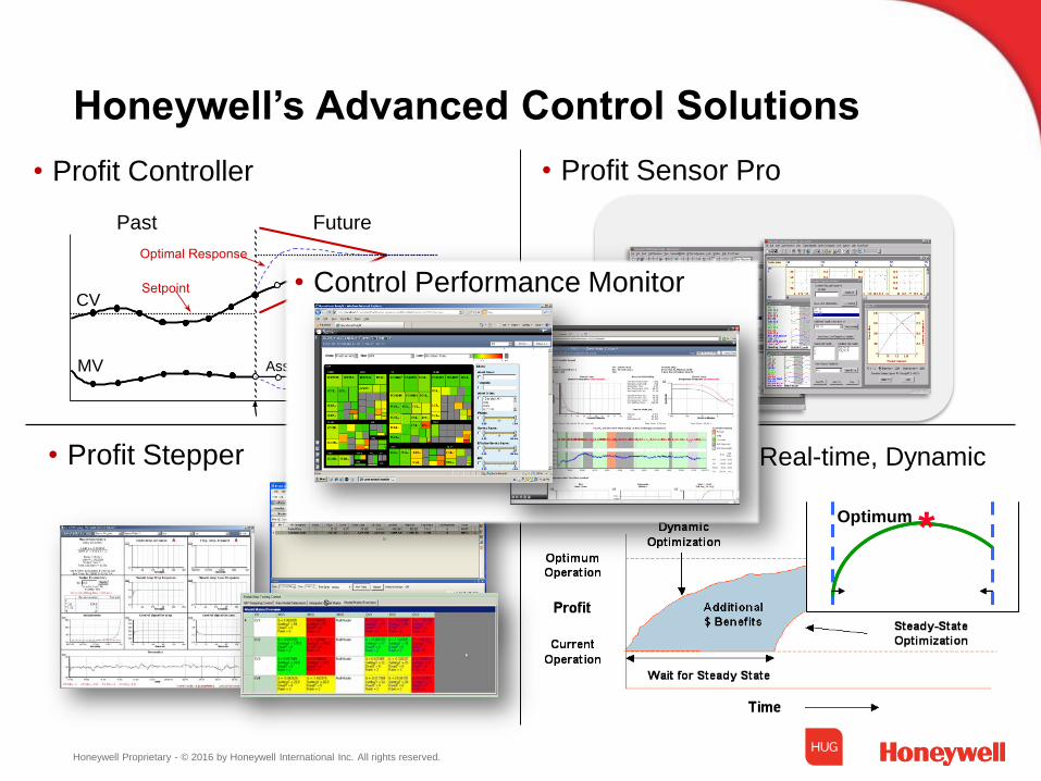
• Profit Stepper
Honeywell’s Advanced Control Solutions
• Profit Controller • Profit Sensor Pro
• Profit Optimizer: Real-time, Dynamic Optimization
*Optimum
Minimum Effort Move
Past Future
Assumed Values
CV
Predicted
Unforced
Response
MV
Control Funnel
Optimal Response
Setpoint • Control Performance Monitor
Honeywell Proprietary - © 2016 by Honeywell International Inc. All rights reserved.
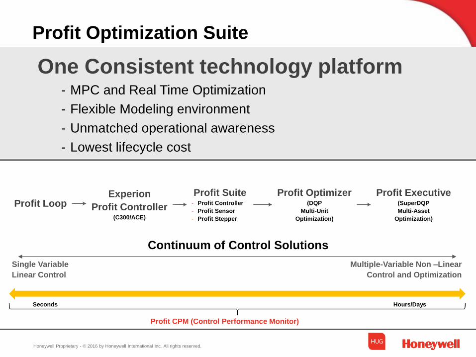
Profit Optimization Suite
One Consistent technology platform- MPC and Real Time Optimization
- Flexible Modeling environment
- Unmatched operational awareness
- Lowest lifecycle cost
Seconds Hours/Days
Profit LoopExperion
Profit Controller(C300/ACE)
Profit Suite- Profit Controller
- Profit Sensor
- Profit Stepper
Profit Optimizer(DQP
Multi-Unit
Optimization)
Profit Executive(SuperDQP
Multi-Asset
Optimization)
Continuum of Control Solutions
Single Variable
Linear Control
Multiple-Variable Non –Linear
Control and Optimization
Profit CPM (Control Performance Monitor)
Honeywell Proprietary - © 2016 by Honeywell International Inc. All rights reserved.
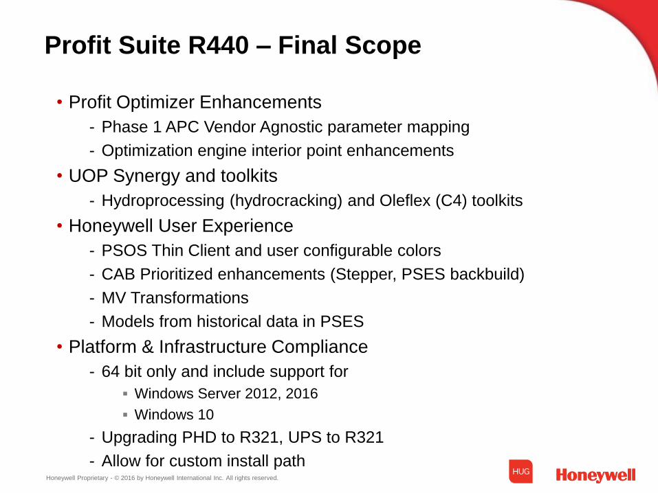
Profit Suite R440 – Final Scope
• Profit Optimizer Enhancements
- Phase 1 APC Vendor Agnostic parameter mapping
- Optimization engine interior point enhancements
• UOP Synergy and toolkits
- Hydroprocessing (hydrocracking) and Oleflex (C4) toolkits
• Honeywell User Experience
- PSOS Thin Client and user configurable colors
- CAB Prioritized enhancements (Stepper, PSES backbuild)
- MV Transformations
- Models from historical data in PSES
• Platform & Infrastructure Compliance
- 64 bit only and include support for
Windows Server 2012, 2016
Windows 10
- Upgrading PHD to R321, UPS to R321
- Allow for custom install path
Honeywell Proprietary - © 2016 by Honeywell International Inc. All rights reserved.
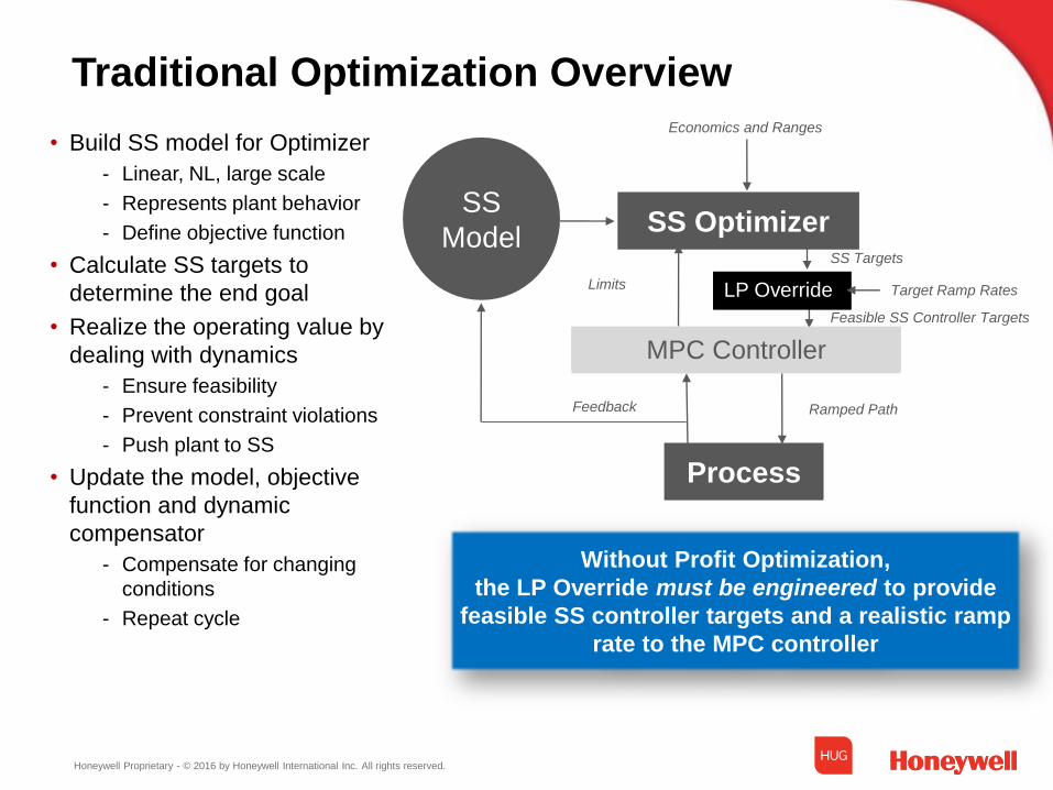
SS Controller TargetsFeasible SS Controller Targets
SS
Model
Traditional Optimization Overview
• Build SS model for Optimizer
- Linear, NL, large scale
- Represents plant behavior
- Define objective function
• Calculate SS targets to
determine the end goal
• Realize the operating value by
dealing with dynamics
- Ensure feasibility
- Prevent constraint violations
- Push plant to SS
• Update the model, objective
function and dynamic
compensator
- Compensate for changing
conditions
- Repeat cycle
SS Optimizer
Economics and Ranges
SS Targets
Process
Dynamic Compensator
Limits
Process Changes
Feasibility
Feedback
LP Override Target Ramp Rates
Without Profit Optimization,
the LP Override must be engineered to provide
feasible SS controller targets and a realistic ramp
rate to the MPC controller
MPC Controller
Ramped Path
Honeywell Proprietary - © 2016 by Honeywell International Inc. All rights reserved.
Honeywell Optimization Solutions
-5 -4 -3 -2 -1 0 1 2 3 4 5-5
-4
-3
-2
-1
0
1
2
3
4
5
x1
x2
Minimization of the JAE function
Start Point
Solution
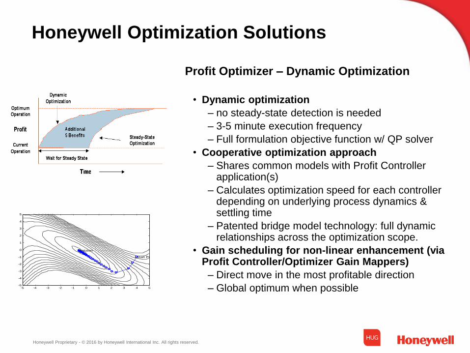
Profit Optimizer – Dynamic Optimization
• Dynamic optimization
– no steady-state detection is needed
– 3-5 minute execution frequency
– Full formulation objective function w/ QP solver
• Cooperative optimization approach
– Shares common models with Profit Controller application(s)
– Calculates optimization speed for each controller depending on underlying process dynamics & settling time
– Patented bridge model technology: full dynamic relationships across the optimization scope.
• Gain scheduling for non-linear enhancement (via Profit Controller/Optimizer Gain Mappers)
– Direct move in the most profitable direction
– Global optimum when possible
Honeywell Proprietary - © 2016 by Honeywell International Inc. All rights reserved.
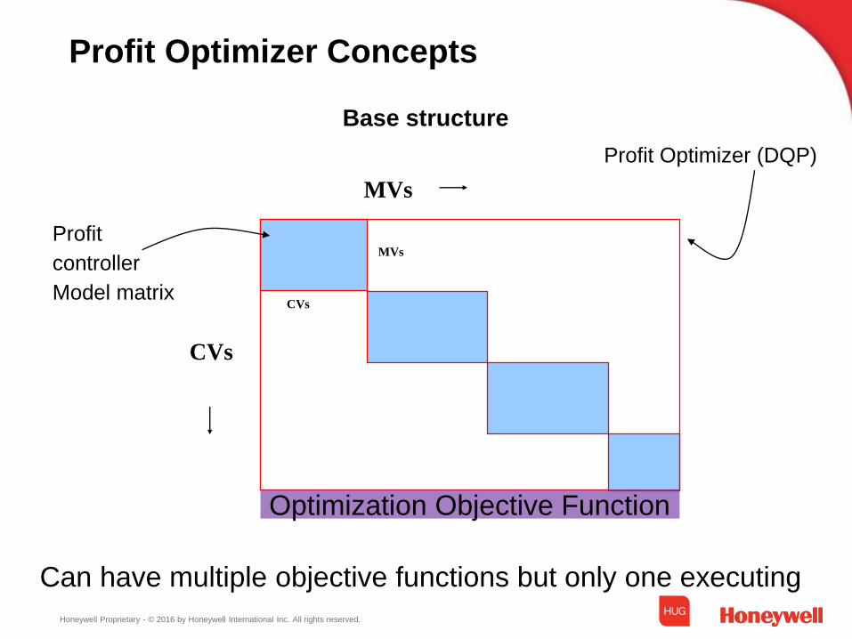
Profit Optimizer Concepts
Profit
controller
Model matrix
MVs
CVs
Base structure
Optimization Objective Function
Can have multiple objective functions but only one executing
Profit Optimizer (DQP)
MVs
CVs
Honeywell Proprietary - © 2016 by Honeywell International Inc. All rights reserved.
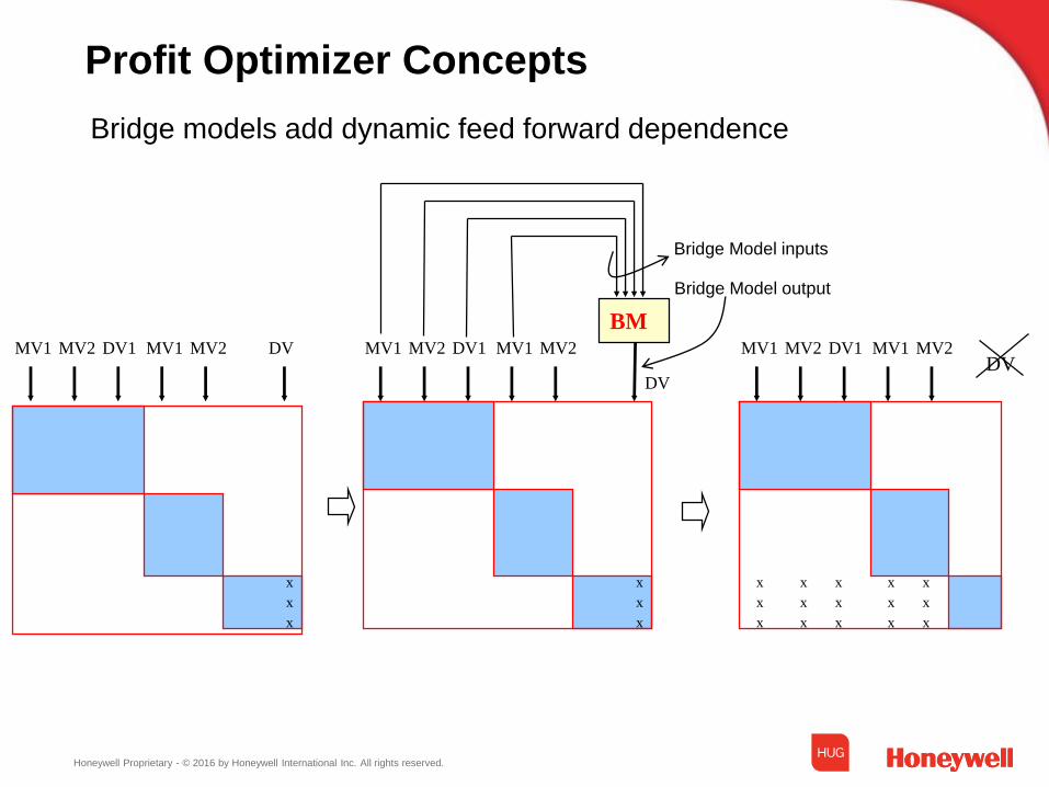
Profit Optimizer Concepts
DV1 DV
x
x
x
MV1 MV2 MV1 MV2 DV1DV
x
x
x
MV1 MV2 MV1 MV2
x
x
x
x
x
x
x
x
x
x
x
x
DV1
DV
x
x
x
MV1 MV2 MV1 MV2
BM
Bridge models add dynamic feed forward dependence
Bridge Model inputs
Bridge Model output
Honeywell Proprietary - © 2016 by Honeywell International Inc. All rights reserved.
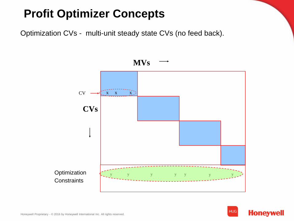
Profit Optimizer Concepts
MVs
CVs
y y y y y y yOptimization
Constraints
• Optimization CVs - multi-unit steady state CVs (no feed back).
CV x x x
Honeywell Proprietary - © 2016 by Honeywell International Inc. All rights reserved.
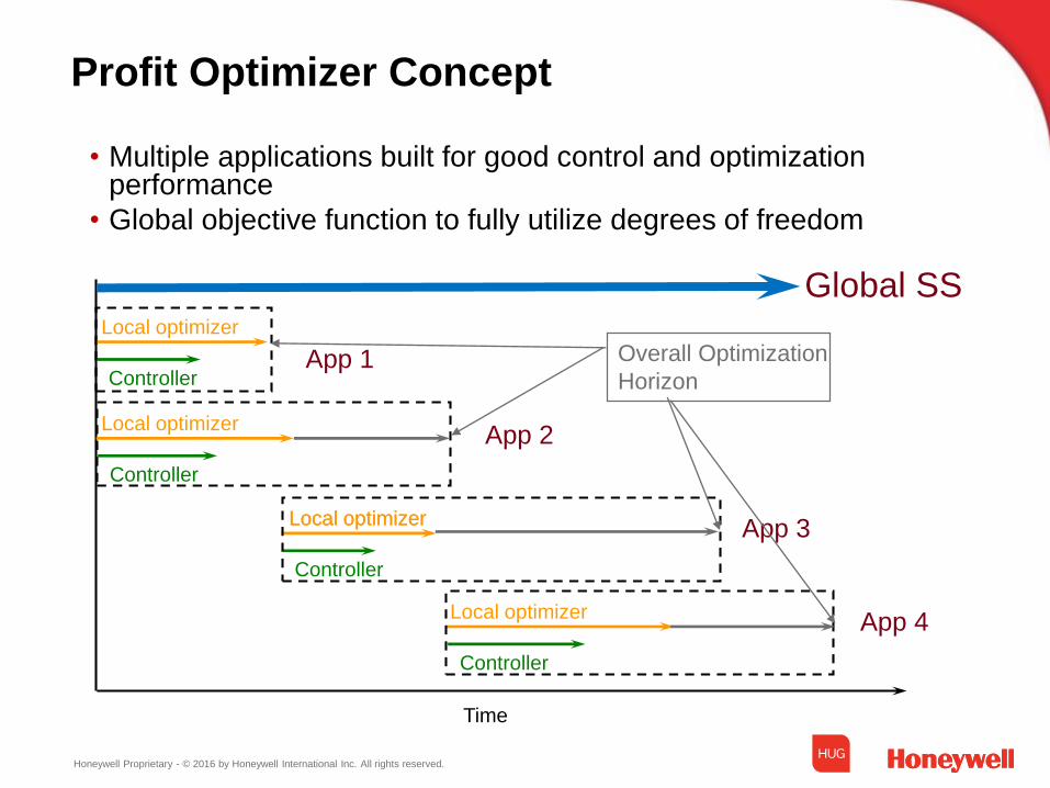
Profit Optimizer Concept
• Multiple applications built for good control and optimization performance
• Global objective function to fully utilize degrees of freedom
Time
Controller
Local optimizer
App 1
Controller
Local optimizerApp 2
Controller
Local optimizer App 3
Controller
Local optimizer App 4
Global SS
Overall Optimization
Horizon
Local optimizer
Honeywell Proprietary - © 2016 by Honeywell International Inc. All rights reserved.
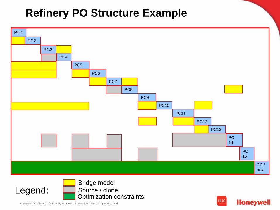
Refinery PO Structure Example
PC1
PC2
PC6
PC7
PC5
PC4
PC8
PC3
PC9
PC10
PC11
PC12
PC13
PC
14
PC
15
CC /
aux
Legend:Optimization constraints
Bridge model
Source / clone
Honeywell Proprietary - © 2016 by Honeywell International Inc. All rights reserved.
Profit Controller 2
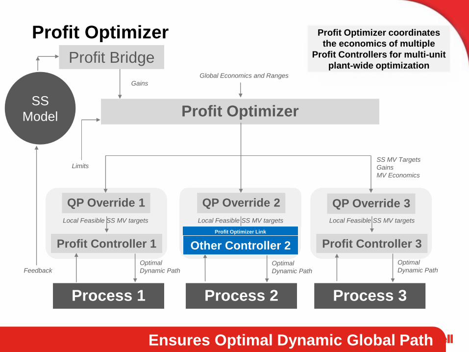
Profit Optimizer
Ensures Optimal Dynamic Global Path
Profit Optimizer
Profit Controller 1
Global Economics and Ranges
SS MV Targets
Gains
MV Economics
Process 1
Profit Controller 3
Process 3Process 2
Limits
Optimal
Dynamic Path
Local Feasible SS MV targets
QP Override 1 QP Override 2 QP Override 3
Feedback
SS
Model
Profit Bridge
Gains
Profit Optimizer Link
Other Controller 2
Profit Optimizer coordinates
the economics of multiple
Profit Controllers for multi-unit
plant-wide optimization
Optimal
Dynamic Path
Optimal
Dynamic Path
Local Feasible SS MV targets Local Feasible SS MV targets
Honeywell Proprietary - © 2016 by Honeywell International Inc. All rights reserved.
-5 -4 -3 -2 -1 0 1 2 3 4 5-5
-4
-3
-2
-1
0
1
2
3
4
5
x1
x2
Minimization of the JAE function
Start Point
Solution
1
65
43 2
7
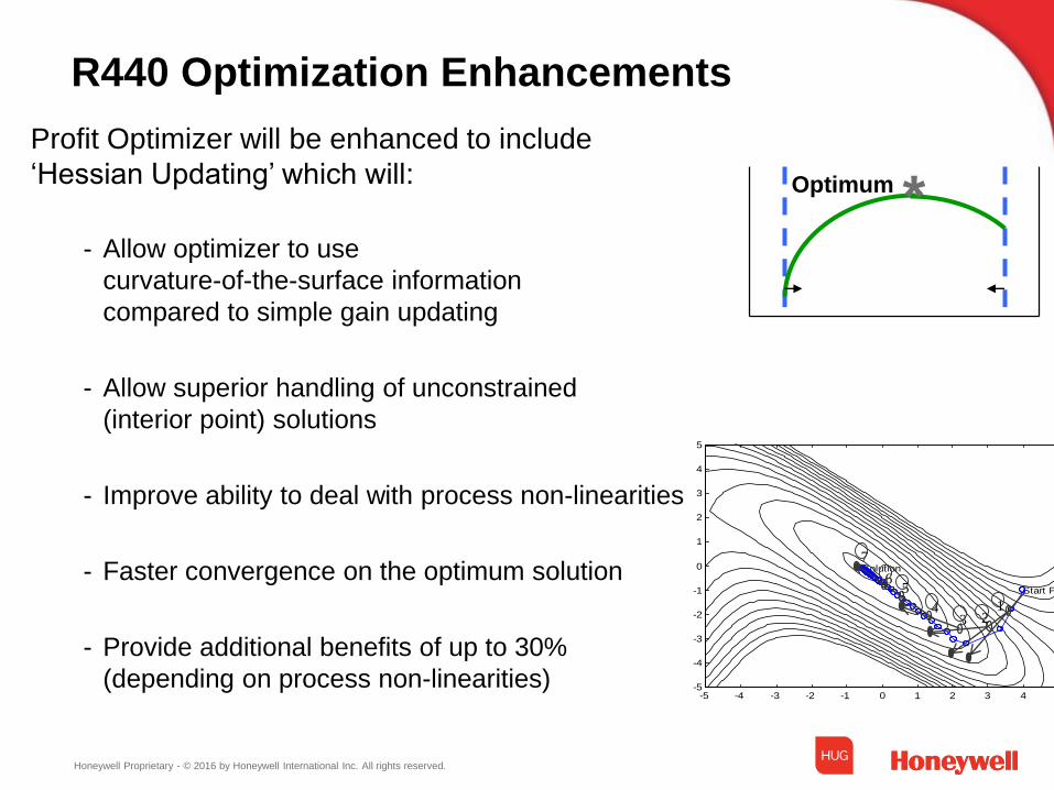
Profit Optimizer will be enhanced to include
‘Hessian Updating’ which will:
- Allow optimizer to use
curvature-of-the-surface information
compared to simple gain updating
- Allow superior handling of unconstrained
(interior point) solutions
- Improve ability to deal with process non-linearities
- Faster convergence on the optimum solution
- Provide additional benefits of up to 30%
(depending on process non-linearities)
R440 Optimization Enhancements
*Optimum
Honeywell Proprietary - © 2016 by Honeywell International Inc. All rights reserved.
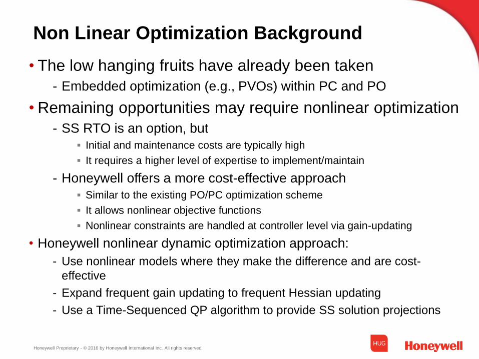
Non Linear Optimization Background
• The low hanging fruits have already been taken
- Embedded optimization (e.g., PVOs) within PC and PO
• Remaining opportunities may require nonlinear optimization
- SS RTO is an option, but
Initial and maintenance costs are typically high
It requires a higher level of expertise to implement/maintain
- Honeywell offers a more cost-effective approach
Similar to the existing PO/PC optimization scheme
It allows nonlinear objective functions
Nonlinear constraints are handled at controller level via gain-updating
• Honeywell nonlinear dynamic optimization approach:
- Use nonlinear models where they make the difference and are cost-
effective
- Expand frequent gain updating to frequent Hessian updating
- Use a Time-Sequenced QP algorithm to provide SS solution projections
Honeywell Proprietary - © 2016 by Honeywell International Inc. All rights reserved.
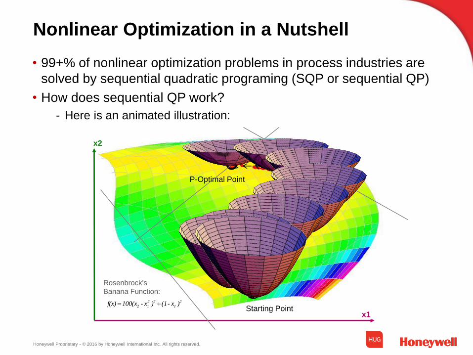
Starting Point
x2
x1
P-Optimal Point
)x-(1)x-100(x f(x) 2
1
22
12
Rosenbrock's
Banana Function:
• 99+% of nonlinear optimization problems in process industries are
solved by sequential quadratic programing (SQP or sequential QP)
• How does sequential QP work?
- Here is an animated illustration:
Nonlinear Optimization in a Nutshell
Honeywell Proprietary - © 2016 by Honeywell International Inc. All rights reserved.
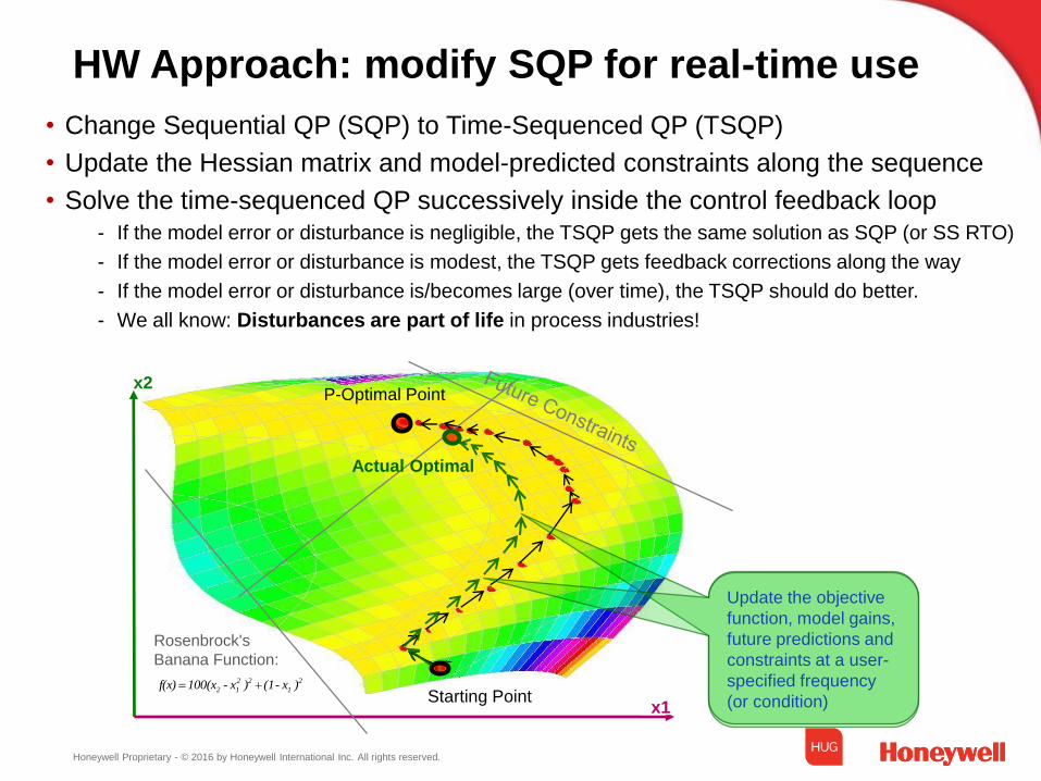
Starting Point
x2
x1
)x-(1)x-100(x f(x) 2
1
22
12
Rosenbrock's
Banana Function:
• Change Sequential QP (SQP) to Time-Sequenced QP (TSQP)
• Update the Hessian matrix and model-predicted constraints along the sequence
• Solve the time-sequenced QP successively inside the control feedback loop- If the model error or disturbance is negligible, the TSQP gets the same solution as SQP (or SS RTO)
- If the model error or disturbance is modest, the TSQP gets feedback corrections along the way
- If the model error or disturbance is/becomes large (over time), the TSQP should do better.
- We all know: Disturbances are part of life in process industries!
HW Approach: modify SQP for real-time use
Update the objective
function, model gains,
future predictions and
constraints at a user-
specified frequency
(or condition)
Actual Optimal
P-Optimal Point
Honeywell Proprietary - © 2016 by Honeywell International Inc. All rights reserved.
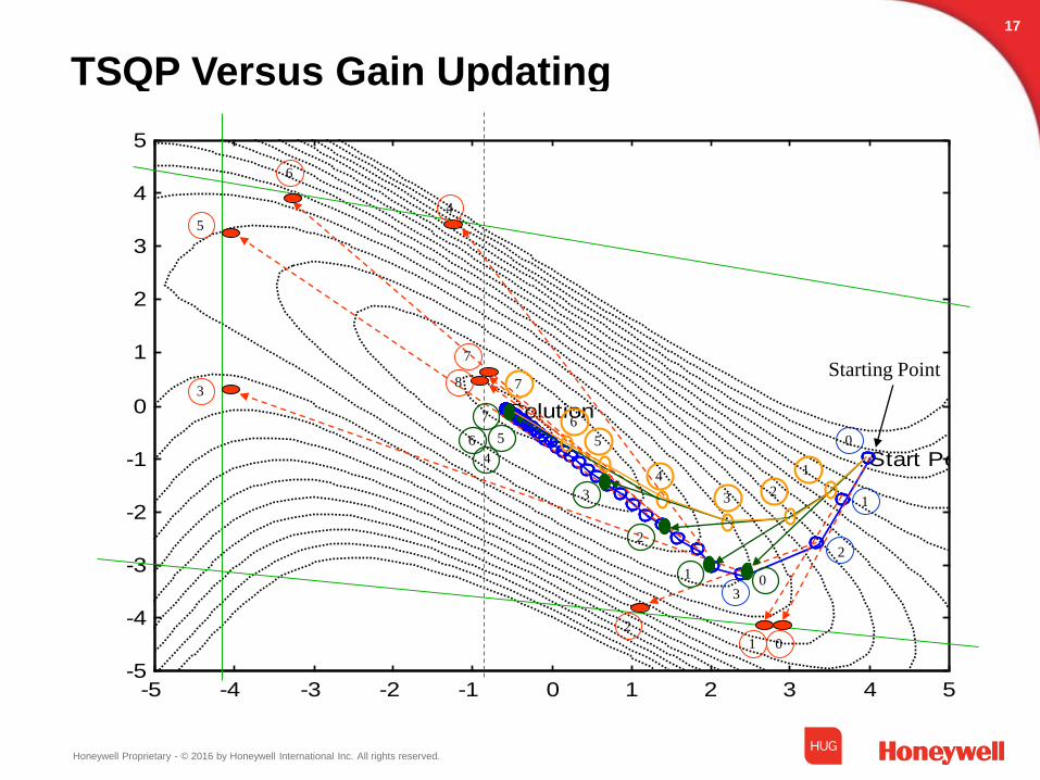
TSQP Versus Gain Updating
17
-5 -4 -3 -2 -1 0 1 2 3 4 5-5
-4
-3
-2
-1
0
1
2
3
4
5
x1
x2Minimization of the JAE function
Start Point
Solution
2
1
01
2
3
4
5
0
6
7
8
3
Starting Point
1
6
5
4
3 2
7
1
6 5
4
3
2
7
0
Honeywell Proprietary - © 2016 by Honeywell International Inc. All rights reserved.
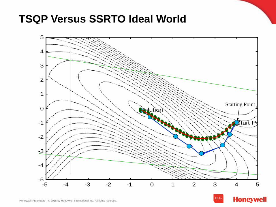
TSQP Versus SSRTO Ideal World
-5 -4 -3 -2 -1 0 1 2 3 4 5-5
-4
-3
-2
-1
0
1
2
3
4
5
x1
x2Minimization of the JAE function
Start Point
SolutionStarting Point
Honeywell Proprietary - © 2016 by Honeywell International Inc. All rights reserved.
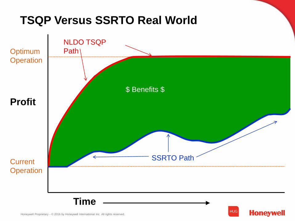
TSQP Versus SSRTO Real World
Time
Optimum
Operation
Current
Operation
Profit
NLDO TSQP
Path
SSRTO Path
$ Benefits $
Honeywell Proprietary - © 2016 by Honeywell International Inc. All rights reserved.
Naphtha
Crude Light Distillate VGO Purchase - Column V
Unit C3/C4 to Poly/Alky
A Vacuum LVGOl Gasoline
Light Gasoil to FCC Tower FCC
HVGO LCO
Heavy Gasoil to FCC A
Vacuum Bottoms to FCC Volumetric HCO
Atmos Bottoms Gain
~111%
Atmos Bottoms to FCC Slurry
Naphtha LCO from FCC
Crude
Unit Heavy Distillate Naphtha
Diesel
B HTR
Diesel
Atmos Bottoms Volumetric Cloud = -5 ~-25C Blending
Gain Sulfur = 0~10ppm
104% Final Product
Naphtha
Naphtha
Crude Light Distillate Diesel Cloud = -45 ~ -48C
Unit Unifiner Sulfur = 4-6ppm
Heavy Distillate
C Volumetric
Atmos Gasoil Gain
101% Debut Overhead
Light Naphtha Debutanizer
Hydro Heavy Naphtha
Atmos Bottoms Vacuum Light Vacuum Gasoil Cracker
Tower Light Distillate
C Heavy Vacuum Gasoil
Heavy Distillate (to FCC)
Volumetric
Vacuum Tower Bottoms Gain Bottoms
HCO from FCC 120%
Component
Tank A
Tank B
Component
FeedTanks 3
Fd tank 2
Feed
Tank 2
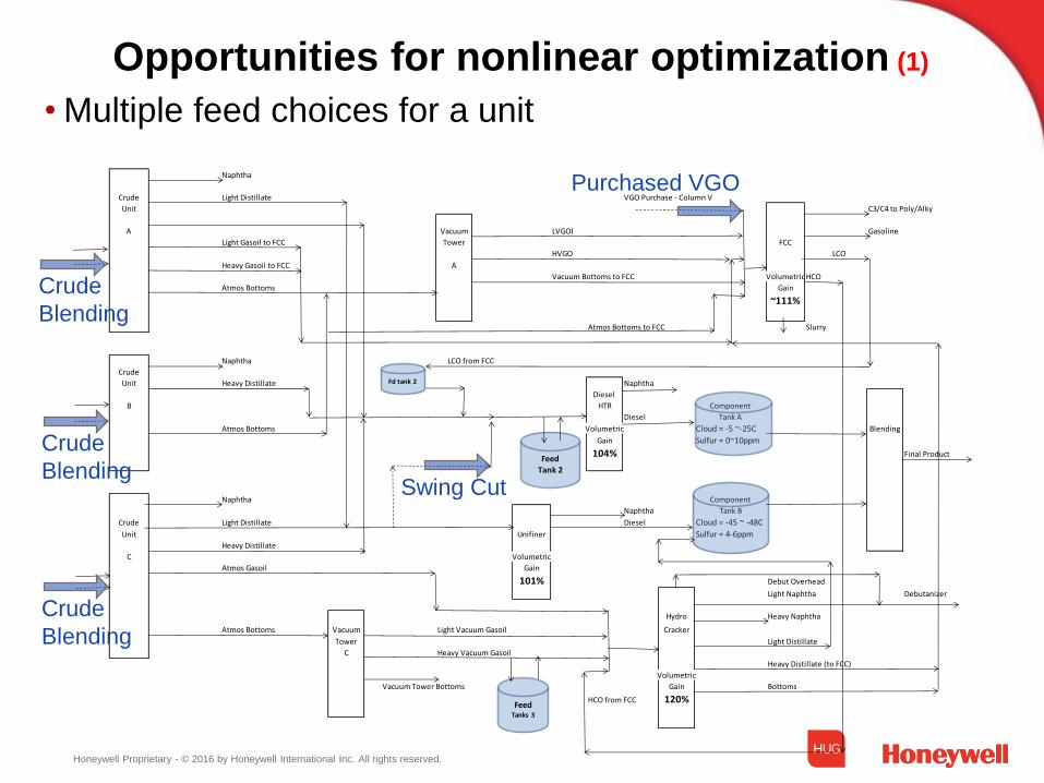
Opportunities for nonlinear optimization (1)
• Multiple feed choices for a unit
Swing Cut
Purchased VGO
Crude
Blending
Crude
Blending
Crude
Blending
Honeywell Proprietary - © 2016 by Honeywell International Inc. All rights reserved.
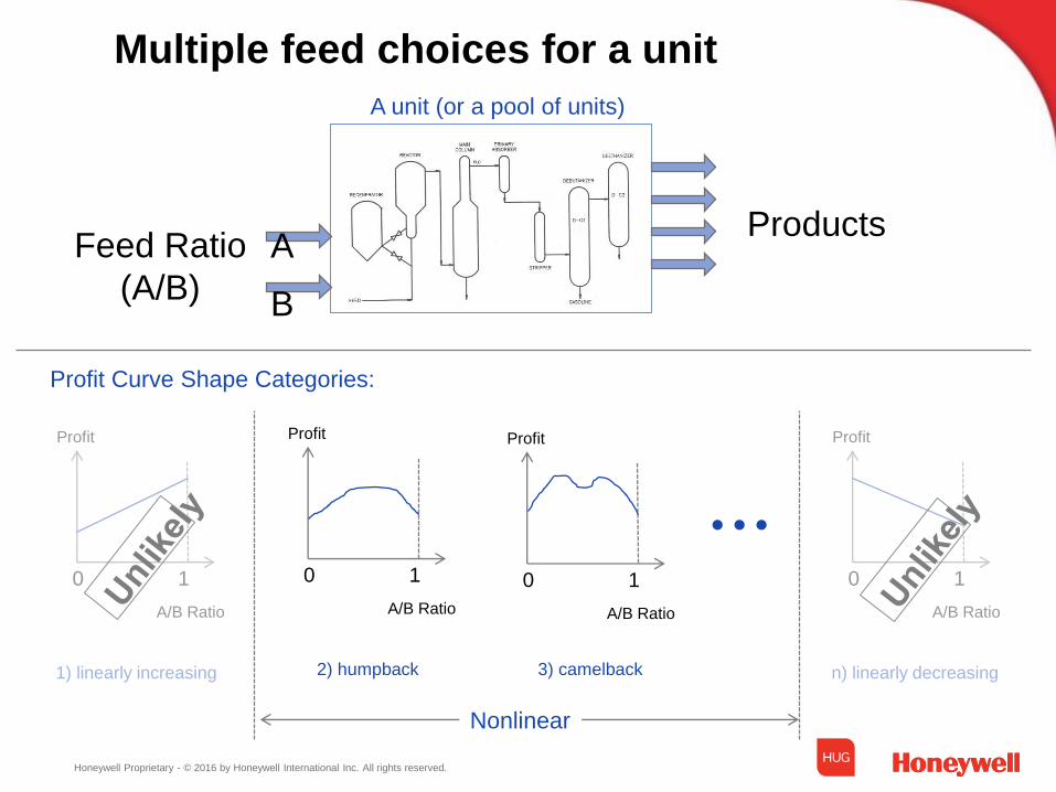
Multiple feed choices for a unit
A
B
Products
A unit (or a pool of units)
0 1
A/B Ratio
Profit
1) linearly increasing
0 1
A/B Ratio
Profit
n) linearly decreasing
0 1
A/B Ratio
Profit
2) humpback
0 1
A/B Ratio
Profit
3) camelback
• • •
Profit Curve Shape Categories:
Nonlinear
Feed Ratio
(A/B)
Honeywell Proprietary - © 2016 by Honeywell International Inc. All rights reserved.
Naphtha
Crude Light Distillate VGO Purchase - Column V
Unit C3/C4 to Poly/Alky
A Vacuum LVGOl Gasoline
Light Gasoil to FCC Tower FCC
HVGO LCO
Heavy Gasoil to FCC A
Vacuum Bottoms to FCC Volumetric HCO
Atmos Bottoms Gain
~111%
Atmos Bottoms to FCC Slurry
Naphtha LCO from FCC
Crude
Unit Heavy Distillate Naphtha
Diesel
B HTR
Diesel
Atmos Bottoms Volumetric Cloud = -5 ~-25C Blending
Gain Sulfur = 0~10ppm
104% Final Product
Naphtha
Naphtha
Crude Light Distillate Diesel Cloud = -45 ~ -48C
Unit Unifiner Sulfur = 4-6ppm
Heavy Distillate
C Volumetric
Atmos Gasoil Gain
101% Debut Overhead
Light Naphtha Debutanizer
Hydro Heavy Naphtha
Atmos Bottoms Vacuum Light Vacuum Gasoil Cracker
Tower Light Distillate
C Heavy Vacuum Gasoil
Heavy Distillate (to FCC)
Volumetric
Vacuum Tower Bottoms Gain Bottoms
HCO from FCC 120%
Component
Tank A
Tank B
Component
FeedTanks 3
Fd tank 2
Feed
Tank 2
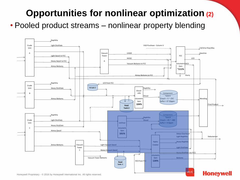
Opportunities for nonlinear optimization (2)
• Pooled product streams – nonlinear property blending
Honeywell Proprietary - © 2016 by Honeywell International Inc. All rights reserved.
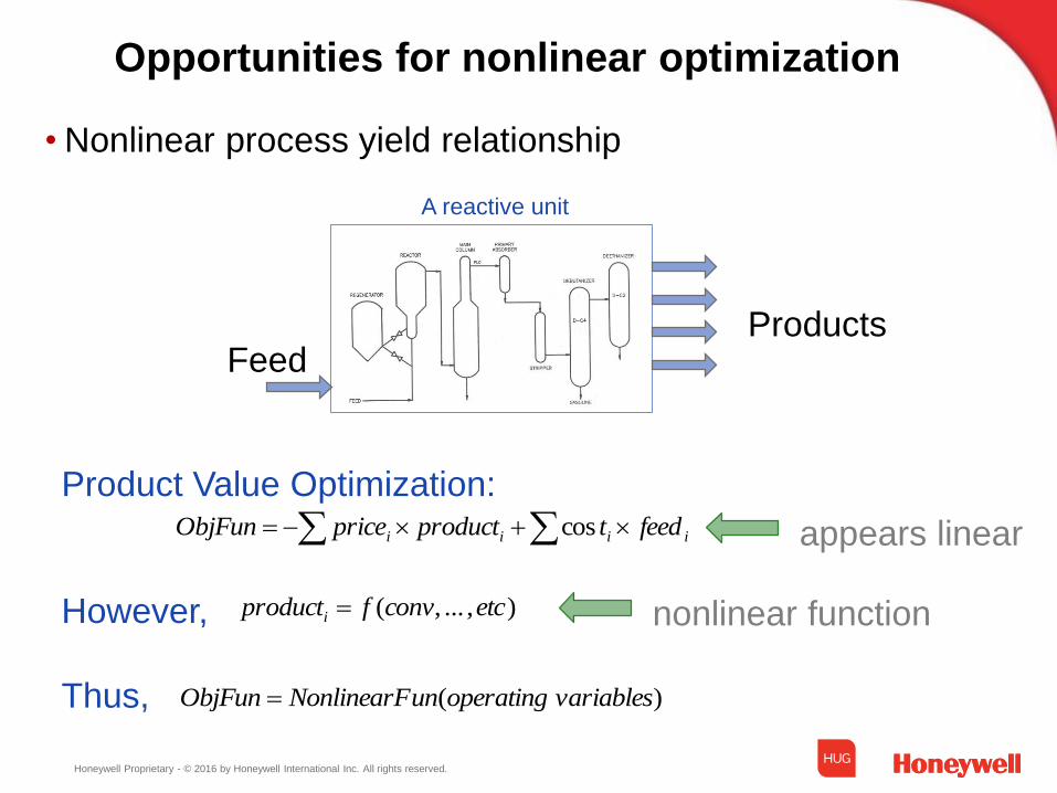
Opportunities for nonlinear optimization
• Nonlinear process yield relationship
Products
A reactive unit
Feed
Product Value Optimization:
However,
Thus,
iiii feedtproductpriceObjFun cos
),...,( etc convfproducti
appears linear
nonlinear function
)( variables operatingunNonlinearFObjFun
Honeywell Proprietary - © 2016 by Honeywell International Inc. All rights reserved.
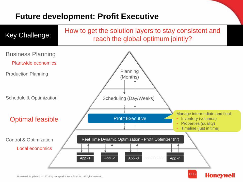
Future development: Profit Executive
Plantwide economics
Local economics
Optimal feasible
Control & Optimization
Schedule & Optimization
Production Planning
Business Planning
Planning
(Months)
Scheduling (Day/Weeks)
Profit Executive
App -1 App -2 App -3 App -n
Real Time Dynamic Optimization - Profit Optimizer (hr)
Key Challenge:How to get the solution layers to stay consistent and
reach the global optimum jointly?
Manage intermediate and final:
• Inventory (volumes)
• Properties (quality)
• Timeline (just in time)
Honeywell Proprietary - © 2016 by Honeywell International Inc. All rights reserved.
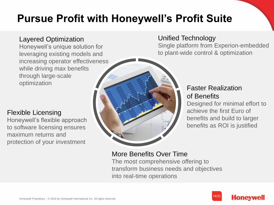
Pursue Profit with Honeywell’s Profit Suite
Unified TechnologySingle platform from Experion-embedded
to plant-wide control & optimization
Faster Realization
of BenefitsDesigned for minimal effort to
achieve the first Euro of
benefits and build to larger
benefits as ROI is justified
More Benefits Over TimeThe most comprehensive offering to
transform business needs and objectives
into real-time operations
Flexible LicensingHoneywell’s flexible approach
to software licensing ensures
maximum returns and
protection of your investment
Layered OptimizationHoneywell’s unique solution for
leveraging existing models and
increasing operator effectiveness
while driving max benefits
through large-scale
optimization


![INDEX [meanwell.com]meanwell.com/Upload/PDF/meanwell_LED.pdf · APC-8, APC-12, APC-16, APC-25, APC-35 3 APV-8E, APV-12E, APV-16E 4 APC-8E, APC-12E, APC-16E LP ... Over voltage protection](https://img.pdfslide.us/doc/110x75/5b619e107f8b9a40488c919f/index-apc-8-apc-12-apc-16-apc-25-apc-35-3-apv-8e-apv-12e-apv-16e-4.jpg)