Embed Size (px)
Citation preview

Profiling relational data: a survey
The MIT Faculty has made this article openly available. Please share how this access benefits you. Your story matters.
Citation Abedjan, Ziawasch, Lukasz Golab, and Felix Naumann. “ProfilingRelational Data: A Survey.” The VLDB Journal 24.4 (2015): 557–581.
As Published http://dx.doi.org/10.1007/s00778-015-0389-y
Publisher Springer Berlin Heidelberg
Version Author's final manuscript
Citable link http://hdl.handle.net/1721.1/106176
Terms of Use Article is made available in accordance with the publisher'spolicy and may be subject to US copyright law. Please refer to thepublisher's site for terms of use.

The VLDB Journal (2015) 24:557–581DOI 10.1007/s00778-015-0389-y
REGULAR PAPER
Profiling relational data: a survey
Ziawasch Abedjan1 · Lukasz Golab2 · Felix Naumann3
Received: 1 August 2014 / Revised: 5 May 2015 / Accepted: 13 May 2015 / Published online: 2 June 2015© Springer-Verlag Berlin Heidelberg 2015
Abstract Profiling data to determine metadata about agiven dataset is an important and frequent activity of anyIT professional and researcher and is necessary for vari-ous use-cases. It encompasses a vast array of methods toexamine datasets and produce metadata. Among the simplerresults are statistics, such as the number of null values anddistinct values in a column, its data type, or the most frequentpatterns of its data values. Metadata that are more difficultto compute involve multiple columns, namely correlations,unique column combinations, functional dependencies, andinclusion dependencies. Further techniques detect condi-tional properties of the dataset at hand. This survey providesa classification of data profiling tasks and comprehensivelyreviews the state of the art for each class. In addition, wereview data profiling tools and systems from research andindustry. We conclude with an outlook on the future of dataprofiling beyond traditional profiling tasks and beyond rela-tional databases.
B Felix [email protected]
Ziawasch [email protected]
Lukasz [email protected]
1 MIT CSAIL, Cambridge, MA, USA
2 University of Waterloo, Waterloo, Canada
3 Hasso Plattner Institute, Potsdam, Germany
1 Data profiling: finding metadata
Data profiling is the set of activities and processes to deter-mine the metadata about a given dataset. Profiling data isan important and frequent activity of any IT professionaland researcher. We can safely assume that any reader of thisarticle has engaged in the activity of data profiling, at leastby eye-balling spreadsheets, database tables, XML files, etc.Possibly, more advanced techniques were used, such as key-word searching indatasets,writing structuredqueries, or evenusing dedicated data profiling tools.
Johnson gives the following definition: “Data profilingrefers to the activity of creating small but informative sum-maries of a database” [79]. Data profiling encompasses a vastarray of methods to examine datasets and produce metadata.Among the simpler results are statistics, such as the numberof null values and distinct values in a column, its data type,or the most frequent patterns of its data values. Metadatathat are more difficult to compute involve multiple columns,such as inclusion dependencies or functional dependencies.Also of practical interest are approximate versions of thesedependencies, in particular because they are typically moreefficient to compute. In this survey we preclude these andconcentrate on exact methods.
Like many data management tasks, data profiling facesthree challenges: (i) managing the input, (ii) performing thecomputation, and (iii) managing the output. Apart from typ-ical data formatting issues, the first challenge addresses theproblem of specifying the expected outcome, i.e., determin-ingwhichprofiling tasks to execute onwhichparts of the data.In fact, many tools require a precise specification of what toinspect. Other approaches aremore open and perform awiderrange of tasks, discovering all metadata automatically.
The second challenge is the main focus of this survey andthat of most research in the area of data profiling: The com-
123
558 Z. Abedjan et al.
putational complexity of data profiling algorithms dependson the number or rows, with a sort being a typical opera-tion, but also on the number of columns. Many tasks needto inspect all column combinations, i.e., they are exponen-tial in the number of columns. In addition, the scalability ofdata profiling methods is important, as the ever-growing datavolumes demand disk-based and distributed processing.
The third challenge is arguably the most difficult, namelymeaningfully interpreting the data profiling results. Obvi-ously, any discovered metadata refer only to the given datainstance and cannot be used to derive schematic/semanticproperties with certainty, such as value domains, primarykeys, or foreignkey relationships. Thus, profiling results needinterpretation, which is usually performed by database anddomain experts.
Tools and algorithms have tackled these challenges indifferent ways. First, many rely on the capabilities of theunderlying DBMS, as many profiling tasks can be expressedas SQL queries. Second, many have developed innovativeways to handle the individual challenges, for instance usingindexing schemes, parallel processing, and reusing interme-diate results. Third, several methods have been proposed thatdeliver only approximate results for various profiling tasks,for instance by profiling samples. Finally, usersmay be askedto narrow down the discovery process to certain columnsor tables. For instance, there are tools that verify inclusiondependencies on user-suggested pairs of columns, but cannotautomatically check inclusion between all pairs of columnsor column sets.
Systematic data profiling, i.e., profiling beyond the occa-sional exploratory SQL query or spreadsheet browsing, isusually performed with dedicated tools or components, suchas IBM’s Information Analyzer, Microsoft’s SQL ServerIntegration Services (SSIS), or Informatica’s Data Explorer.1
These approaches follow the same general procedure: Auser specifies the data to be profiled and selects the typesof metadata to be generated. Next, the tool computes themetadata in batch mode, using SQL queries and/or spe-cialized algorithms. Depending on the volume of the dataand the selected profiling results, this step can last minutesto hours. Results are usually displayed in a vast collec-tion of tabs, tables, charts, and other visualizations to beexplored by the user. Typically, discoveries can then betranslated to constraints or rules that are then enforced ina subsequent cleansing/integration phase. For instance, afterdiscovering that themost frequent pattern for phone numbersis (ddd)ddd-dddd, this pattern can be promoted to a rulestating that all phone numbers must be formatted accord-ingly. Most data cleansing tools can then either transformdifferently formatted numbers or mark them as improper.
1 See Sect. 6 for a more comprehensive list of tools.
We focus our discussion on relational data, the predomi-nant format of traditional data profiling methods, but we docover data profiling for other data models in Sect. 7.2.
1.1 Use-cases for data profiling
Data profiling has many traditional use-cases, including thedata exploration, data cleansing, and data integration scenar-ios. Statistics about data are also useful in query optimization.Finally we describe several domain-specific use-cases, suchas scientific data management and big data analytics.
Data exploration Database administrators, researchers, anddevelopers are often confronted with new datasets, aboutwhich they know nothing. Examples include data files down-loaded from the Web, old database dumps, or newly gainedaccess to some DBMS. In many cases, such data have noknown schema, no or old documentation, etc. Even if a for-mal schema is specified, it might be incomplete, for instancespecifying only the primary keys but no foreign keys. A nat-ural first step is to understand how the data are structured,what they are about, and how much of them there are.
Such manual data exploration, or data gazing2, can andshould be supported with data profiling techniques. Simple,ad hoc SQL queries can reveal some insight, such as thenumber of distinct values, but more sophisticated methodsare needed to efficiently and systematically discover meta-data. Furthermore, we cannot always expect an SQL expertas the explorer, but rather “data enthusiasts” without formalcomputer science training [68]. Thus, automated data profil-ing is needed to provide a basis for further analysis. Mortonet al. [107] recognize that a key challenge is overcomingthe current assumption of data exploration tools that data are“clean and in a well-structured relational format.” Often datacannot be analyzed and visualized as is.
Database management A basic form of data profiling is theanalysis of individual columns in a given table. Typically, thegenerated metadata include various counts, such as the num-ber of values, the number of unique values, and the numberof non-null values. These metadata are often part of the basicstatistics gathered by a DBMS. An optimizer uses them toestimate the selectivity of operators and perform other opti-mization steps. Mannino et al. [99] give a survey of statisticscollection and its relationship to database optimization.Moreadvanced techniques use histograms of value distributions,functional dependencies, and unique column combinationsto optimize range queries [118] or for dynamic reoptimiza-tion [80].
2 “Data gazing involves looking at the data and trying to reconstructa story behind these data. […] Data gazing mostly uses deduction andcommon sense.” [104]
123

Profiling relational data: a survey 559
Database reverse engineering Given a “bare” databaseinstance, the task of schema and database reverse engineer-ing is to identify its relations and attributes, as well as domainsemantics, such as foreign keys and cardinalities [103,116].Hainaut et al. [66] call these metadata “implicit constructs,”i.e., those that are not explicitly specified byDDL statements.However, possible sources for reverse engineering are DDLstatements, data instances, data dictionaries, etc. The result ofreverse engineering might be an entity-relationship model ora logical schema to assist experts in maintaining, integrating,and querying the database.
Data integration Often, the datasets to be integrated areunfamiliar and the integration expert wants to explore thedatasets first: How large are they? What data types areneeded? What are the semantics of columns and tables? Arethere dependencies between tables and among databases?,etc. The vast abundance of (linked) open data and the desireand potential to integrate them with local data has amplifiedthis need.
A concrete use-case for data profiling is that of schemamatching, i.e., finding semantically correct correspondencesbetween elements of two schemata [44]. Many schemamatching systems perform data profiling to create attributefeatures, such as data type, average value length, and pat-terns, to compare feature vectors and align those attributeswith the best matching ones [98,109].
Scientific data management and integration have cre-ated additional motivation for efficient and effective dataprofiling: When importing raw data, e.g., from scientificexperiments or extracted from the Web, into a DBMS, it isoften necessary and useful to profile the data and then devisean adequate schema. In many cases, scientific data are pro-duced by non-database experts and without the intention toenable integration. Thus, they often come with no adequateschematic information, such as data types, keys, or foreignkeys.
Apart from exploring individual sources, data profilingcan also reveal how and how well two datasets can be inte-grated. For instance, inclusion dependencies across tablesfromdifferent sources suggestwhich tablesmight reasonablybe combined with a join operation. Additionally, specializeddata profiling techniques can reveal how much two relationsoverlap in their intent and extent.We discuss these challengesin Sect. 7.1.
Data quality / data cleansing The need to profile a new orunfamiliar set of data arises in many situations, in general toprepare for some subsequent task. A typical use-case is pro-filing data to prepare a data cleansing process. Commercialdata profiling tools are usually bundled with correspondingdata quality / data cleansing software.
Profiling as a data quality assessment tool reveals dataerrors, such as inconsistent formattingwithin a column,miss-ing values, or outliers. Profiling results can also be used tomeasure and monitor the general quality of a dataset, forinstance by determining the number of records that do notconform to previously established constraints [81,117]. Gen-erated constraints and dependencies also allow for rule-baseddata imputation.
Big data analytics “Big data,” with its high volume, highvelocity, and high variety [90], are data that cannot be man-aged with traditional techniques. Thus, data profiling gains anew importance. Fetching, storing, querying, and integratingbig data are expensive, despite many modern technologies:Before exposing an infrastructure to Twitter’s firehose, itmight be worthwhile to know about properties of the dataone is receiving; before downloading significant parts of thelinked data cloud, some prior sense of the integration effortis needed; before augmenting a warehouse with text min-ing results an understanding of its data quality is required.In this context, leading researchers have noted “If we justhave a bunch of datasets in a repository, it is unlikely anyonewill ever be able to find, let alone reuse, any of these data.With adequate metadata, there is some hope, but even so,challenges will remain[…] [7].”
Many big data and related data science scenarios call fordata mining and machine learning techniques to explore andmine data. Again, data profiling is an important preparatorytask to determine which data to mine, how to import it intothe various tools, and how to interpret the results [120].
Further use-cases Knowledge about data types, keys, for-eign keys, and other constraints supports data modeling andhelps keep data consistent, improves query optimization, andreaps all the other benefits of structured data management.Others havementioned query formulation and indexing [126]and scientific discovery [75] as further motivation for dataprofiling. Also, compression techniques internally performbasic data profiling to optimize the compression ratio.Finally, the areas of data governance and data life-cyclemanagement are becoming more and more relevant to busi-nesses trying to adhere to regulations and code. Especiallyconcerned are financial institutions and health care organiza-tions. Again, data profiling can help ascertain which actionsto take on which data.
1.2 Article overview and contributions
Data profiling is an important and practical topic that isclosely connected to several other data management areas. Itis also a timely topic and is becoming increasingly importantgiven the recent trends in data science and big data analyt-ics [108]. While it may not yet be a mainstream term in the
123
560 Z. Abedjan et al.
database community, there already exists a large body ofwork that directly and indirectly addresses various aspectsof data profiling. The goal of this survey is to classify anddescribe this body of work and illustrate its relevance to data-base research and practice.We also show that data profiling isfar from a “done deal” and identify several promising direc-tions for future work in this area.
The remainder of this paper is organized as follows. InSect. 2, we outline and define data profiling based on anew taxonomy of profiling tasks. Sections 3, 4, and 5 sur-vey the state of the art of the three main research areas indata profiling: analysis of individual columns, analysis ofmultiple columns, and detection of dependencies betweencolumns, respectively. Section 6 surveys data profiling toolsfrom research and industry. We provide an outlook of dataprofiling challenges in Sect. 7 and conclude this survey inSect. 8.
2 Profiling tasks
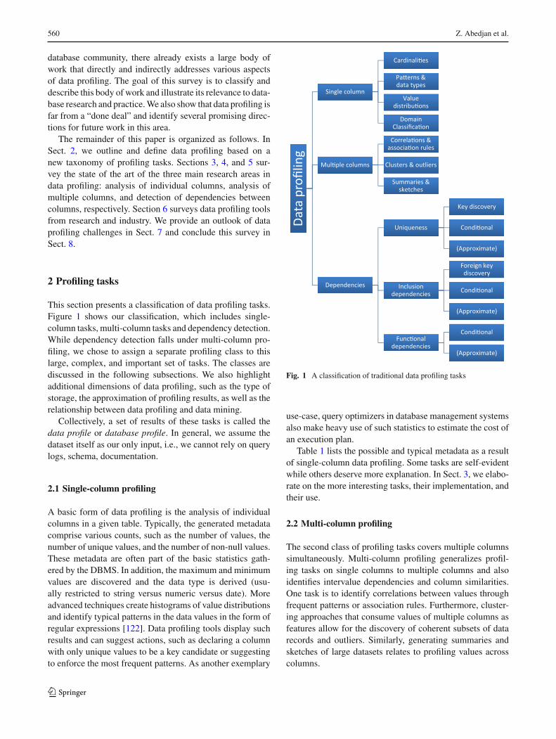
This section presents a classification of data profiling tasks.Figure 1 shows our classification, which includes single-column tasks, multi-column tasks and dependency detection.While dependency detection falls under multi-column pro-filing, we chose to assign a separate profiling class to thislarge, complex, and important set of tasks. The classes arediscussed in the following subsections. We also highlightadditional dimensions of data profiling, such as the type ofstorage, the approximation of profiling results, as well as therelationship between data profiling and data mining.
Collectively, a set of results of these tasks is called thedata profile or database profile. In general, we assume thedataset itself as our only input, i.e., we cannot rely on querylogs, schema, documentation.
2.1 Single-column profiling
A basic form of data profiling is the analysis of individualcolumns in a given table. Typically, the generated metadatacomprise various counts, such as the number of values, thenumber of unique values, and the number of non-null values.These metadata are often part of the basic statistics gath-ered by the DBMS. In addition, the maximum and minimumvalues are discovered and the data type is derived (usu-ally restricted to string versus numeric versus date). Moreadvanced techniques create histograms of value distributionsand identify typical patterns in the data values in the form ofregular expressions [122]. Data profiling tools display suchresults and can suggest actions, such as declaring a columnwith only unique values to be a key candidate or suggestingto enforce the most frequent patterns. As another exemplary
Data
pro
filin
g
Single column
Cardinali�es
Pa�erns &data types
Value distribu�ons
Domain Classifica�on
Mul�ple columns
Correla�ons & associa�on rules
Clusters & outliers
Summaries & sketches
Dependencies
Uniqueness
Key discovery
Condi�onal
(Approximate)
Inclusion dependencies
Foreign key discovery
Condi�onal
(Approximate)
Func�onal dependencies
Condi�onal
(Approximate)
Fig. 1 A classification of traditional data profiling tasks
use-case, query optimizers in database management systemsalso make heavy use of such statistics to estimate the cost ofan execution plan.
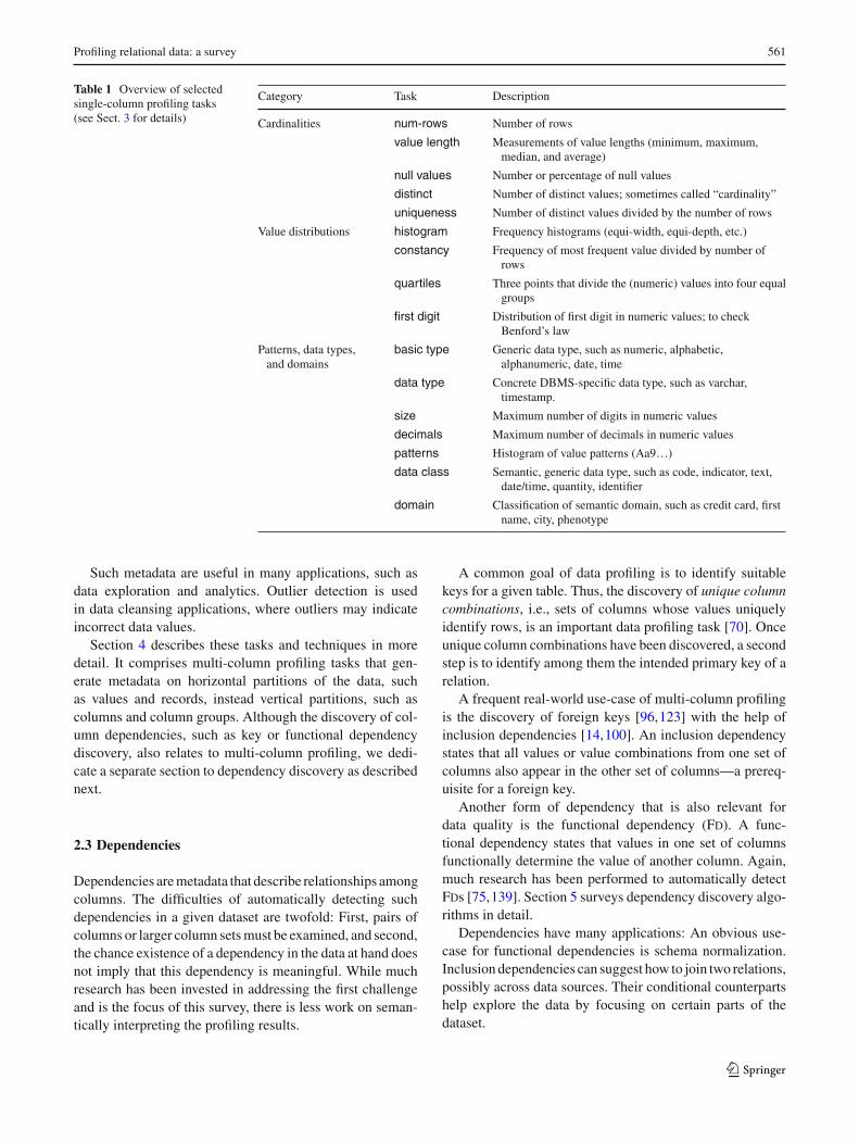
Table 1 lists the possible and typical metadata as a resultof single-column data profiling. Some tasks are self-evidentwhile others deserve more explanation. In Sect. 3, we elabo-rate on the more interesting tasks, their implementation, andtheir use.
2.2 Multi-column profiling
The second class of profiling tasks covers multiple columnssimultaneously. Multi-column profiling generalizes profil-ing tasks on single columns to multiple columns and alsoidentifies intervalue dependencies and column similarities.One task is to identify correlations between values throughfrequent patterns or association rules. Furthermore, cluster-ing approaches that consume values of multiple columns asfeatures allow for the discovery of coherent subsets of datarecords and outliers. Similarly, generating summaries andsketches of large datasets relates to profiling values acrosscolumns.
123
Profiling relational data: a survey 561
Table 1 Overview of selectedsingle-column profiling tasks(see Sect. 3 for details)
Category Task Description
Cardinalities num-rows Number of rows
value length Measurements of value lengths (minimum, maximum,median, and average)
null values Number or percentage of null values
distinct Number of distinct values; sometimes called “cardinality”
uniqueness Number of distinct values divided by the number of rows
Value distributions histogram Frequency histograms (equi-width, equi-depth, etc.)
constancy Frequency of most frequent value divided by number ofrows
quartiles Three points that divide the (numeric) values into four equalgroups
first digit Distribution of first digit in numeric values; to checkBenford’s law
Patterns, data types,and domains
basic type Generic data type, such as numeric, alphabetic,alphanumeric, date, time
data type Concrete DBMS-specific data type, such as varchar,timestamp.
size Maximum number of digits in numeric values
decimals Maximum number of decimals in numeric values
patterns Histogram of value patterns (Aa9…)
data class Semantic, generic data type, such as code, indicator, text,date/time, quantity, identifier
domain Classification of semantic domain, such as credit card, firstname, city, phenotype
Such metadata are useful in many applications, such asdata exploration and analytics. Outlier detection is usedin data cleansing applications, where outliers may indicateincorrect data values.
Section 4 describes these tasks and techniques in moredetail. It comprises multi-column profiling tasks that gen-erate metadata on horizontal partitions of the data, suchas values and records, instead vertical partitions, such ascolumns and column groups. Although the discovery of col-umn dependencies, such as key or functional dependencydiscovery, also relates to multi-column profiling, we dedi-cate a separate section to dependency discovery as describednext.
2.3 Dependencies
Dependencies aremetadata that describe relationships amongcolumns. The difficulties of automatically detecting suchdependencies in a given dataset are twofold: First, pairs ofcolumns or larger column setsmust be examined, and second,the chance existence of a dependency in the data at hand doesnot imply that this dependency is meaningful. While muchresearch has been invested in addressing the first challengeand is the focus of this survey, there is less work on seman-tically interpreting the profiling results.
A common goal of data profiling is to identify suitablekeys for a given table. Thus, the discovery of unique columncombinations, i.e., sets of columns whose values uniquelyidentify rows, is an important data profiling task [70]. Onceunique column combinations have been discovered, a secondstep is to identify among them the intended primary key of arelation.
A frequent real-world use-case of multi-column profilingis the discovery of foreign keys [96,123] with the help ofinclusion dependencies [14,100]. An inclusion dependencystates that all values or value combinations from one set ofcolumns also appear in the other set of columns—a prereq-uisite for a foreign key.
Another form of dependency that is also relevant fordata quality is the functional dependency (Fd). A func-tional dependency states that values in one set of columnsfunctionally determine the value of another column. Again,much research has been performed to automatically detectFds [75,139]. Section 5 surveys dependency discovery algo-rithms in detail.
Dependencies have many applications: An obvious use-case for functional dependencies is schema normalization.Inclusion dependencies can suggest how to join two relations,possibly across data sources. Their conditional counterpartshelp explore the data by focusing on certain parts of thedataset.
123
562 Z. Abedjan et al.
2.4 Conditional, partial, and approximate solutions
Real datasets usually contain exceptions to rules. To accountfor this, dependencies and other constraints detected by dataprofiling can be relaxed. We describe two relaxations below:partial and approximate.
Partial dependencies hold for only a subset of the records,for instance, for 95% of the records or for all but 10 records.Such dependencies are especially valuable in data cleansingscenarios: They are patterns that hold for almost all recordsand thus should probably hold for all records if the data wereclean. Violating records can be extracted and cleansed [129].
Once a partial dependency has been detected, it is inter-esting to characterize for which records it holds, i.e., if wecan find a condition that selects precisely those records.Conditional dependencies can specify such conditions. Forinstance, a conditional unique column combination mightstate that the column street is unique for all records with city= ‘NY.’ Conditional inclusion dependencies (Cinds) wereproposed by Bravo et al. for data cleaning and contextualschema matching [19]. Conditional functional dependencies(Cfds) were introduced in [46], also for data cleaning.
Approximate dependencies and other constraints areunconditional statements, but are not guaranteed to hold forthe entire relation. Such dependencies are often discoveredusing sampling [76] or other summarization techniques [31].Their approximate nature is often sufficient for certain tasks,and approximate dependencies can be used as input to themore rigorous task of detecting true dependencies. This sur-vey does not discuss such approximation techniques.
2.5 Types of storage
Data profiling tasks are applicable to a wide range of sit-uations in which data are provided in various forms. Forinstance, most commercial profiling tools assume that datareside in a relational database, make use of SQL queries andindexes. In other situations, for instance, a csv file is providedand a data profilingmethod needs to create its own data struc-tures inmemory or on disk. And finally, there are situations inwhich a mixed approach is useful: Data that were originallyin the database are read once and processed further outsidethe database.
The discussion and distinction of such different situa-tions is relevant when evaluating the performance of dataprofiling algorithms and tools. Can we assume that data arealready loaded into main memory? Can we assume the pres-ence of indices? Are profiling results, which can be quitevoluminous, written to disk? Fair comparisons need to estab-lish a level playing field with same assumptions about datastorage.
2.6 Data profiling versus data mining
A clear, well-defined, and accepted distinction between dataprofiling and data mining does not exist. Two criteria areconceivable:
1. Distinction by the object of analysis: instance versusschema or columns versus rows
2. Distinction by the goal of the task: description of existingdata versus new insights beyond existing data.
Following thefirst criterion,RahmandDodistinguish dataprofiling from data mining by the number of columns that areexamined: “Data profiling focuses on the instance analysisof individual attributes. […] Data mining helps discover spe-cific data patterns in large datasets, e.g., relationships holdingbetween several attributes” [121]. While this distinction iswell defined, we believe several tasks, such as Ind or Fddetection, belong to data profiling, even if they discover rela-tionships between multiple columns.
We believe a different distinction along both criteria ismore useful: Data profiling gathers technical metadata tosupport data management; data mining and data analyticsdiscovers non-obvious results to support business manage-ment with new insights. While data profiling focuses mainlyon columns, some data mining tasks, such as rule discoveryor clustering, may also be used for identifying interestingcharacteristics of a dataset. Others, such as recommendationor classification, are not related to data profiling.
With this distinction, we concentrate on data profilingand put aside the broad area of data mining, which hasalready received unifying treatment in numerous textbooksand surveys. However, in Sect. 4, we address the subsetof unsupervised mining approaches that can be applied onunknown data to generate metadata and hence serves the pur-pose of data profiling.
Classifications of data mining tasks include an overviewby Chen et al., who distinguish the kinds of databases (rela-tional, OO, temporal, etc.), the kinds of knowledge to bemined (association rules, clustering, deviation analysis, etc.),and the kinds of techniques to be used [130]. Wemake a sim-ilar distinction in this survey. In particular, we distinguishthe different classes of data profiling tasks and then exam-ine various techniques to perform them.We discuss profilingnon-relational data in Sect. 7.
2.7 Summary
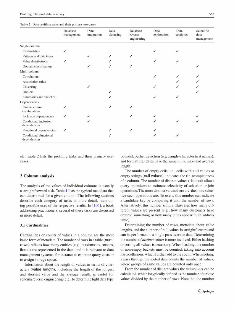
We summarize this section by connecting the various dataprofiling tasks with the use-cases mentioned in the introduc-tion. Conceivably, any task can be useful for any use-case,depending on the context, the properties of the data at hand,
123
Profiling relational data: a survey 563
Table 2 Data profiling tasks and their primary use-cases
Databasemanagement
Dataintegration
Datacleansing
Databasereverseengineering
Dataexploration
Dataanalytics
Scientificdatamanagement
Single-column
Cardinalities ✓ ✓ ✓
Patterns and data types ✓ ✓ ✓
Value distributions ✓ ✓ ✓ ✓
Domain classification ✓ ✓ ✓ ✓
Multi-column
Correlations ✓ ✓ ✓
Association rules ✓ ✓
Clustering ✓ ✓ ✓ ✓
Outliers ✓ ✓
Summaries and sketches ✓ ✓ ✓
Dependencies
Unique columncombinations
✓ ✓ ✓
Inclusion dependencies ✓ ✓ ✓ ✓ ✓
Conditional inclusiondependencies
✓ ✓ ✓ ✓
Functional dependencies ✓ ✓ ✓ ✓
Conditional functionaldependencies
✓ ✓ ✓
etc. Table 2 lists the profiling tasks and their primary use-cases.
3 Column analysis
The analysis of the values of individual columns is usuallya straightforward task. Table 1 lists the typical metadata thatcan determined for a given column. The following sectionsdescribe each category of tasks in more detail, mention-ing possible uses of the respective results. In [104], a bookaddressing practitioners, several of these tasks are discussedin more detail.
3.1 Cardinalities
Cardinalities or counts of values in a column are the mostbasic form of metadata. The number of rows in a table (num-rows) reflects how many entities (e.g., customers, orders,items) are represented in the data, and it is relevant to datamanagement systems, for instance to estimate query costs orto assign storage space.
Information about the length of values in terms of char-acters (value length), including the length of the longestand shortest value and the average length, is useful forschema reverse engineering (e.g., to determine tight data type
bounds), outlier detection (e.g., single-character first names),and formatting (dates have the same min-, max- and averagelength).
The number of empty cells, i.e., cells with null values orempty strings (null values), indicates the (in-)completenessof a column. The number of distinct values (distinct) allowsquery optimizers to estimate selectivity of selection or joinoperations:Themore distinct values there are, themore selec-tive such operations are. To users, this number can indicatea candidate key by comparing it with the number of rows.Alternatively, this number simply illustrates how many dif-ferent values are present (e.g., how many customers haveordered something or how many cities appear in an addresstable).
Determining the number of rows, metadata about valuelengths, and the number of null values is straightforward andcan be performed in a single pass over the data. Determiningthe number ofdistinct values ismore involved:Either hashingor sorting all values is necessary. When hashing, the numberof non-empty buckets must be counted, taking into accounthash collisions, which further add to the count.When sorting,a pass through the sorted data counts the number of values,where groups of same values are counted only once.
From the number of distinct values the uniqueness can becalculated,which is typically defined as the number of uniquevalues divided by the number of rows. Note that the number
123

564 Z. Abedjan et al.
of distinct values can also be estimated using the minHashtechnique discussed in Sect. 4.3.
Apart from determining the exact number of distinct val-ues, query optimization is a strong incentive to estimate thosecounts in order to predict query execution plan costs with-out actually reading the entire data. Because approximateprofiling is not the focus of this survey, we give only twoexemplary pointers. Haas et al. [65] base their estimation ondata samples and describe and empirically compare variousestimators from the literature. Other works do scan the entiredata but use only a small amount of memory to hash thevalues and estimate the number of distinct values, an earlyexample being [11].
3.2 Value distribution
Value distributions are more fine-grained cardinalities,namely the cardinalities of groups of values. Histogramsare among the most common profiling results. A histogramstores frequencies of values within well-defined groups, usu-ally by dividing the ordered set of values into a fixed set ofbuckets. The buckets of equi-width histograms span valueranges of same length, while the buckets of equi-depth (orequi-height) histograms each represent the same number ofvalue occurrences. A common special case of an equi-depthhistogram is dividing the data into four quartiles. A moregeneral concept is biased histograms, which can adapt theiraccuracy for different regions[33]. Histograms are used fordatabase optimization as a rough probability distribution toavoid a uniform distribution assumption and thus providebetter cardinality estimations [77]. In addition, histogramsare interpretable by humans, as their visual representation iseasy to comprehend.
The constancy of a column is defined as the ratio of thefrequency of the most frequent value (possibly a pre-defineddefault value) and the overall number of values. It thus rep-resents the proportion of some constant value compared withthe entire column.
A particularly interesting distribution is the first digit dis-tribution for numeric values. Benford’s law [15] states that innaturally occurring numbers the distribution of the first digitd of a number approximately follows P(d) = log10(1+ 1
d ).Thus, the 1 is expected to be the most frequent leading digit,followed by 2, etc. Benford and others have observed thisbehavior inmany sets of numbers, such asmolecularweights,building sizes, and electricity bills. In fact, the law has beenused to uncover accounting fraud and other fraudulently cre-ated numbers.
Determining the abovedistributions usually involves a sin-gle pass over the column, except for equi-depth histograms(i.e., with fixed bucket sizes) and quartiles, which determinebucket boundaries through sorting. In the same manner or
through hashing the most frequent value can be discoveredto determine constancy.
Finally, many more things can be counted and aggregatedin a column. For instance, some profiling tools and meth-ods determine among others the frequency distribution ofsoundex code, n-grams, and others, the inverse frequency dis-tribution, i.e., the distribution of the frequency distribution,or the entropy of the frequency distribution of the values ina column [82].
3.3 Types and patterns
The profiling tasks of this section are ordered by increasingsemantic richness (see also Table 1). We start with the mostsimple observable properties, move on to specific patterns ofthe values of a column, and end with the semantic domain ofa column.
Discovering the basic type of a column, i.e., classifying itas numeric, alphabetic, alphanumeric, date, or time, is fairlysimple: The presence or absence of numeric and non-numericcharacters already distinguishes the first three. The latter twocan usually be recognized by the presence of numbers onlywithin certain ranges, and by numbers separated in regu-lar patterns by special symbols. Recognizing the actual datatype, for instance among the SQL types, is similarly easy. Infact, data of many data types, such as timestamp, boolean,or int, must follow a fixed, sometimes DBMS-specific pat-tern. When classifying columns into data types, one shouldchoose the most specific data type—in particular avoidingthe catchalls char or varchar if possible. For the data typesdecimal, float, and double, one can additionally extract themaximum number of digits and decimals to determine themetadata size and decimals.
A common and useful data profiling result is the extrac-tion of frequent patterns observed in the data of a col-umn. Then, data that do not conform to such a patternare likely erroneous or ill-formed. For instance, a pat-tern for phone numbers might be informally encoded as+dd (ddd) ddd dddd or as a simple regular expression\(\d3\)\ − \d3\ − \d4).3 A challenge when determiningfrequent patterns is to find a good balance between generalityand specificity. The regular expression.* is themost generaland matches any string. On the other hand, the expressiondata allows only that one single string. For the Potter’sWheel tool, Raman and Hellerstein [122] suggest findingthe data pattern with the minimal description length (MDL).Theymodel description length as a combination of precision,recall, and conciseness and provide an algorithm to enumer-ate all possible patterns. The RelIE system was designed
3 A more detailed regular expression, taking into account different for-matting options and different restrictions (e.g., phone numbers cannotbegin with a 1), can easily reach 200 characters in length.
123

Profiling relational data: a survey 565
for information extraction from textual data [92]. It createsregular expressions based on training data with positive andnegative examples by systematically, greedily transformingregular expressions. Finally, Fernau [51] provides a goodcharacterization of the problem of learning regular expres-sions fromdata and presents a learning algorithm for the task.This work is also a good starting point for further reading
The semantic domain of a column describes not the syntaxof its values but their meaning. While a regular expressionmight characterize a column, labeling it as “phone number”provides a concrete domain. Clearly, this task cannot be fullyautomated, but some work has been done for common-placedomains about persons, places, etc. Zhang et al. take a firststep by clustering columns that have the samemeaning acrossthe tables of a database [144], which they extend to the par-ticularly difficult area of numeric values in [142]. In [133]the authors take the additional step of matching columns topre-defined semantics from the person domain. Knowledgeof the domain is not only of general data profiling interest,but also of particular interest to schema matching, i.e., thetask of finding semantic correspondences between elementsof different database schemata.
3.4 Data completeness
Explicitmissing data are simple to characterize: For each col-umn, we report the number of tuples with a null or a defaultvalue. However, datasets may contain disguised missing val-ues. For example, Web forms often include fields whosevalues must be chosen from pull-down lists. The first valuefrom the pull-down list may be pre-populated on the form,and some users may not replace it with a proper or correctvalue due to lack of time or privacy concerns. Specific exam-ples include entering 99999 as the zip code of an addressor leaving “Alabama” as the pre-populated state (in the US,Alabama is alphabetically the first state). Of course, for somerecords, Alabama may be the true state.
Detecting disguised default values is difficult. One heuris-tic solution is to examine each column at a time, and, for eachpossible value, compute the distribution of the other attributevalues [74]. For example, if Alabama is indeed a disguiseddefault value, we expect a large subset of tuples with state =Alabama (i.e., those whose true state is different) to forman unbiased sample of the whole relation.
Another instance in which profiling missing data is nottrivial involves timestamped data, such as measurement ortransaction data feeds. In some cases, tuples are expected toarrive regularly, e.g., in datacentermonitoring, everymachinemay be configured to report its CPU utilization everyminute.However, measurements may be lost en route to the data-base, and overloaded or malfunctioning machines may notreport any measurements at all. [60]. In contrast to detectingmissing attribute values, here we are interested in estimat-
ing the number of missing tuples. Thus, the profiling taskmay be to single out the columns identified as being of typetimestamp, and, for those that appear to be distributed uni-formly across a range, infer the expected frequency of theunderlying data source and estimate the number of miss-ing tuples. Of course, some timestamp columns correspondto application timestamps with no expectation of regularity,rather than data arrival timestamps. For instance, in an onlineretailer database, order dates and delivery dates are generallynot expected to be scattered uniformly over time.
4 Multi-column analysis
Profiling tasks over a single column can be generalized toprojections of multiple columns. For example, there has beenwork on computing multi-dimensional histograms for queryoptimization [41,119]. Multi-column profiling also playsan important role in data cleansing, e.g., in assessing andexplaining data glitches, which often occur in column com-binations [40].
In the remainder of this section, we discuss statisticalmethods and data mining approaches for generating meta-data based on co-occurrences and dependencies of valuesacross attributes. We focus on correlation and rule miningapproaches as well as unsupervised clustering and learningapproaches; machine learning techniques that require train-ing data or detailed knowledge of the data are beyond thescope of data profiling.
4.1 Correlations and association rules
Correlation analysis reveals related numeric columns, e.g.,in an Employees table, age and salarymay be correlated. Astraightforwardway to do this is to compute pairwise correla-tions among all pairs of columns. In addition to column-levelcorrelations, value-level associations may provide usefuldata profiling information.
Traditionally, a common application of association ruleshas been tofind items that tend to be purchased together basedon point-of-sale transaction data. In these datasets, each rowis a list of items purchased in a given transaction. An associa-tion rule {bread}→ {butter}, for example, states that ifa transaction includes bread, it is also likely to include butter,i.e., customers who buy bread also buy butter. A set of itemsis referred to as an itemset, and an association rule specifiesan itemset on the left-hand side and another itemset on theright-hand side.
Algorithms for generating association rules from datadecompose the problem into two steps [8]:
1. Discover all frequent itemsets, i.e., those whose fre-quencies in the dataset (i.e., their support) exceed some
123
566 Z. Abedjan et al.
threshold. For instance, the itemset {bread, butter}may appear in 800 out of a total of 50,000 transactionsfor a support of 1.6%.
2. For each frequent itemset a, generate association rulesof the form l → a − l with l ⊂ a, whose confidenceexceeds some threshold. Confidence is defined as thefrequency of a divided by the frequency of l, i.e., theconditional probability of l given a − l. For example, ifthe frequency of {bread, butter} is 800 and the fre-quency of {bread} alone is 1000, then the confidenceof the association rule {bread} → {butter} is 0.8.That is, if bread is purchased, there is an 80% chance thatbutter is also purchased in the same transaction.
In the context of relational data profiling, associationrules denote relationships or patterns between attribute val-ues among columns. Consider an Employees table withfields name, employee number, department, position,and allowance. We may find a frequent itemset of theform {department = finance, position = assistantmanager, allowance = $1000} and a corresponding asso-ciation rule of the form {department = finance, position= assistant manager} → {allowance = $1000}.This would be the case if most or all assistant managers inthe finance department were assigned an allowance budgetof $1000.
While the second step mentioned above is straightforward(generating association rules from frequent itemsets), the firststep is computationally expensive due to the large number ofpossible frequent itemsets (or patterns of values) [72]. Pop-ular algorithms for efficiently discovering frequent patternsinclude Apriori [8], Eclat [141], and FP-Growth [67].
The Apriori algorithm exploits the observation that allsubsets of a frequent itemsetmust also be frequent. In the firstiteration, Apriori finds all frequent itemsets of size one, i.e.,those containing one item or one attribute value. In the nextiteration, only the frequent itemsets of size one are expandedto find frequent itemsets of size two, and so on.
There are also several optimized versions of Apriori,such as DHP [115] and RARM [35]. FP-Growth discov-ers frequent itemsets without a candidate generation step.It transforms the database into an extended prefix tree offrequent patterns (FP-tree). The FP-Growth algorithm tra-verses the tree and generates frequent itemsets by patterngrowth in a depth-first manner. Finally, Eclat is based onintersecting transaction-id (TID) sets of associated itemsetsand is best suited for dealing with large frequent itemsets.Eclat’s strategy for identifying frequent itemsets is similar toApriori.
Negative correlation rules, i.e., those that identify attributevalues that do not co-occur with other attribute values, mayalso be useful in data profiling to find anomalies and out-liers [21]. However, discovering negative association rules is
more difficult, because infrequent itemsets cannot be prunedin the same way as frequent itemsets, and therefore, novelpruning rules are required [135].
Finally, we note that in addition to using existing tech-niques, such as correlations and association rules for pro-filing, extensions have been proposed, such as discoveringlinear dependencies between columns [25].
However, in this approach, the user has to choose thesubset of attributes to be analyzed. We discuss dependencydiscovery in more detail in Sect. 5.
4.2 Clustering and outlier detection
Another useful profiling task is to segment the records intohomogeneous groups using a clustering algorithm; further-more, records that do not fit into any cluster may be flaggedas outliers. Cluster analysis can identify groups of similarrecords in a table, while outliers may indicate data qual-ity problems. For example, Dasu and Johnson [36] clusternumeric columns and identify outliers in the data. Further-more, based on the assumption that data glitches occur acrossattributes and not in isolation [16], statistical inference hasbeen applied to measure glitch recovery in [39].
Another example of clustering in the context of data profil-ing is ProLOD++, which applies k-means clustering to Rdfrelations [1]. We refer the reader to surveys by Jain et al. [78]and Xu and Wunsch II [137] for more details on clusteringalgorithms for relational data.
4.3 Summaries and sketches
Besides clustering, another way to describe data is to createsummaries or sketches [23]. This can be done by samplingor hashing data values to a smaller domain. Sketches havebeen widely applied to answering approximate queries, datastream processing and estimating join sizes [37,54,111].Cormode et al. [31] give an overview of sketching and sam-pling for approximate query processing.
Another interesting task is to assess the similarity of twocolumns, which can be done using multi-column hashingtechniques. The Jaccard similarity of two columns A andB is |A ∩ B|/|A ∪ B|, i.e., the number of distinct valuesthey have in common divided by the total number of distinctvalues appearing in them. This gives the relative number ofvalues that appear in both A and B. Since semantically similarvalues may have different formats, we can also compute theJaccard similarity of the n-gram distributions in A and B. Ifthe distinct value sets of columns A and B are not available,we can estimate the Jaccard similarity using their MinHashsignatures [38].
123
Profiling relational data: a survey 567
Table 3 Dependency discoveryalgorithms
Dependency Algorithms
Uniques HCA [3], GORDIAN [126], DUCC [70], SWAN [5]
Functional dependencies TANE [75], FUN [110], FD_Mine [139], Dep-Miner [95],FastFDs [136], FDEP [52], DFD[6]
Conditional functional dependencies [24], [59], CTANE [47], CFUN [42], FACD [91], FastCFD[47]
Inclusion dependencies [101], [87], SPIDER [14], ZigZag [102]
Conditional inclusion dependencies [61], CINDERELLA [13], PLI [13]
Foreign keys [123], [143]
Denial constraints FastDC [29]
Differential dependencies [128]
Sequential dependencies [57]
5 Dependency detection
We now survey various formalisms for detecting depen-dencies among columns and algorithms for mining themfrom data, including keys and unique column combinations(Sect. 5.1), functional dependencies (Sect. 5.2), inclusiondependencies (Sect. 5.3), and other types of dependenciesthat are relevant to data profiling (Sect. 5.4). Table 3 lists thealgorithms that are discussed.
We use the following symbols: R and S denote relationalschemata, with r and s denoting instances of R and S, respec-tively. The number of columns in R is |R| and the number oftuples in r is |r |. We refer to tuples of r and s as ri and s j ,respectively. Subsets of columns are denoted by uppercaseX,Y, Z (with |X | denoting the number of columns in X ) andindividual columns by uppercase A, B,C . Furthermore, wedefine πX (r) and πA(r) as the projection of r on the attributeset X or attribute A, respectively; thus, |πX (r)| denotes thecount of district combinations of the values of X appearingin r . Accordingly, ri [A] indicates the value of the attribute Aof tuple ri and ri [X ] = πX (ri ). We refer to an attribute valueof a tuple as a cell.
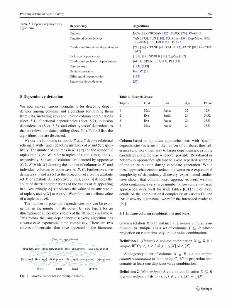
The number of potential dependencies in r can be expo-nential in the number of attributes |R|; see Fig. 2 for anillustration of all possible subsets of the attributes in Table 4.This means that any dependency discovery algorithm hasa worst-case exponential time complexity. There are twoclasses of heuristics that have appeared in the literature.
Fig. 2 Powerset lattice for the example Table 4
Table 4 Example dataset
Tuple id First Last Age Phone
1 Max Payne 32 1234
2 Eve Smith 24 5432
3 Eve Payne 24 3333
4 Max Payne 24 3333
Column-based or top-down approaches start with “small”dependencies (in terms of the number of attributes they ref-erence) and work their way to larger dependencies, pruningcandidates along the way whenever possible. Row-based orbottom-up approaches attempt to avoid repeated scanningof the entire relation during candidate generation. Whilethese approaches cannot reduce the worst-case exponentialcomplexity of dependency discovery, experimental studieshave shown that column-based approaches work well ontables containing a very large number of rows and row-basedapproaches work well for wide tables [6,113]. For moredetails on the computational complexity of various Fd andInd discovery algorithms, we refer the interested reader to[94].
5.1 Unique column combinations and keys
Given a relation R with instance r , a unique column com-bination (a “unique”) is a set of columns X ⊆ R whoseprojection on r contains only unique value combinations.
Definition 1 (Unique) A column combination X ⊆ R is aunique, iff ∀ri , r j ∈ r, i = j : ri [X ] = r j [X ].
Analogously, a set of columns X ⊆ R is a non-uniquecolumn combination (a “non-unique”), iff its projection on rcontains at least one duplicate value combination.
Definition 2 (Non-unique) A column combination X ⊆ Ris a non-unique, iff ∃ri , r j ∈ r, i = j : ri [X ] = r j [X ].
123
568 Z. Abedjan et al.
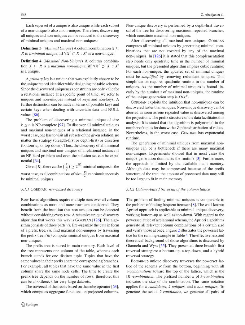
Each superset of a unique is also unique while each subsetof a non-unique is also a non-unique. Therefore, discoveringall uniques and non-uniques can be reduced to the discoveryof minimal uniques and maximal non-uniques:
Definition 3 (Minimal Unique) A column combination X ⊆R is a minimal unique, iff ∀X ′ ⊂ X : X ′ is a non-unique.
Definition 4 (Maximal Non-Unique) A column combina-tion X ⊆ R is a maximal non-unique, iff ∀X ′ ⊃ X : X ′is a unique.
A primary key is a unique that was explicitly chosen to bethe unique record identifierwhile designing the table schema.Since the discovered uniqueness constraints are only valid fora relational instance at a specific point of time, we refer touniques and non-uniques instead of keys and non-keys. Afurther distinction can be made in terms of possible keys andcertain keys when dealing with uncertain data and NULLvalues [86].
The problem of discovering a minimal unique of sizek ≤ n is NP-complete [97]. To discover all minimal uniquesand maximal non-uniques of a relational instance, in theworst case, one has to visit all subsets of the given relation, nomatter the strategy (breadth-first or depth-first) or direction(bottom-up or top-down). Thus, the discovery of all minimaluniques and maximal non-uniques of a relational instance isan NP-hard problem and even the solution set can be expo-nential [64].
Given |R|, there canbe (|R||R|2
) ≥ 2|R|2 minimal uniques in the
worst case, as all combinations of size |R|2 can simultaneously
be minimal uniques.
5.1.1 Gordian: row-based discovery
Row-based algorithms require multiple runs over all columncombinations as more and more rows are considered. Theybenefit from the intuition that non-uniques can be detectedwithout considering every row. A recursive unique discoveryalgorithm that works this way is Gordian [126]. The algo-rithm consists of three parts: (i) Pre-organize the data in formof a prefix tree, (ii) find maximal non-uniques by traversingthe prefix tree, (iii) compute minimal uniques from maximalnon-uniques.
The prefix tree is stored in main memory. Each level ofthe tree represents one column of the table, whereas eachbranch stands for one distinct tuple. Tuples that have thesame values in their prefix share the corresponding branches.For example, all tuples that have the same value in the firstcolumn share the same node cells. The time to create theprefix tree depends on the number of rows; therefore, thiscan be a bottleneck for very large datasets.
The traversal of the tree is based on the cube operator [63],which computes aggregate functions on projected columns.
Non-unique discovery is performed by a depth-first traver-sal of the tree for discovering maximum repeated branches,which constitute maximal non-uniques.
After discovering all maximal non-uniques, Gordiancomputes all minimal uniques by generating minimal com-binations that are not covered by any of the maximalnon-uniques. In [126] it is stated that this complementationstep needs only quadratic time in the number of minimaluniques, but the presented algorithm implies cubic runtime:For each non-unique, the updated set of minimal uniquesmust be simplified by removing redundant uniques. Thissimplification requires quadratic runtime in the number ofuniques. As the number of minimal uniques is bound lin-early by the number s of maximal non-uniques, the runtimeof the unique generation step is O(s3).
Gordian exploits the intuition that non-uniques can bediscovered faster than uniques. Non-unique discovery can beaborted as soon as one repeated value is discovered amongthe projections. The prefix structure of the data facilitates thisanalysis. It is stated that the algorithm is polynomial in thenumber of tuples for datawith aZipfiandistribution of values.Nevertheless, in the worst case, Gordian has exponentialruntime.
The generation of minimal uniques from maximal non-uniques can be a bottleneck if there are many maximalnon-uniques. Experiments showed that in most cases theunique generation dominates the runtime [3]. Furthermore,the approach is limited by the available main memory.Although data may be compressed because of the prefixstructure of the tree, the amount of processed data may stillbe too large to fit in main memory.
5.1.2 Column-based traversal of the column lattice
The problem of finding minimal uniques is comparable tothe problem of finding frequent itemsets [8]. Thewell-knownApriori approach is applicable to minimal unique discovery,working bottom-up as well as top-down. With regard to thepowerset lattice of a relational schema, theApriori algorithmsgenerate all relevant column combinations of a certain sizeand verify those at once. Figure 2 illustrates the powerset lat-tice for the running example in Table 4. The effectiveness andtheoretical background of those algorithms is discussed byGiannela and Wyss [55]. They presented three breadth-firsttraversal strategies: a bottom-up, a top-down, and a hybridtraversal strategy.
Bottom-up unique discovery traverses the powerset lat-tice of the schema R from the bottom, beginning with all1-combinations toward the top of the lattice, which is the|R|-combination. The prefixed number k of k-combinationindicates the size of the combination. The same notationapplies for k-candidates, k-uniques, and k-non-uniques. Togenerate the set of 2-candidates, we generate all pairs of
123

Profiling relational data: a survey 569
1-non-uniques. k-candidates with k > 2 are generated byextending the (k − 1)-non-uniques by another non-uniquecolumn. After the candidate generation, each candidate ischecked for uniqueness. If it is identified as a non-unique,the k-candidate is added to the list of k-non-uniques.
If the candidate is verified as unique, its minimalityhas to be checked. The algorithm terminates when k =|1-non-uniques|. A disadvantage of this candidate generationtechnique is that redundant uniques and duplicate candidatesare generated and tested.
The Apriori idea can also be applied to the top-downapproach. Having the set of identified k-uniques, one hasto verify whether the uniques are minimal. Therefore, foreach k-unique, all possible (k − 1)-subsets have to be gener-ated and verified. The hybrid approach generates the kth and(n−k)th levels simultaneously. Experiments have shown thatin most datasets, uniques usually occur in the lower levels ofthe lattice, which favors bottom-up traversal [3].
Hca is an improved version of the bottom-up Aprioritechnique [3]. Hca optimizes the candidate generation step,applies statistical pruning and considers functional depen-dencies that have been inferred on the fly. In terms ofcandidate generation, Hca applies the optimized join thatwas introduced for frequent itemset mining [8]. Hca gener-ates candidates by combining only (k − 1)-non-uniques thatshare the first k − 2 elements. If no such two non-uniquesexist, no candidates are generated and the algorithm termi-nates before reaching the last level of the powerset lattice.Further pruning can be achieved by considering value his-tograms and distinct counts that can be retrieved on the fly inprevious levels. For example, consider the1-non-uniques lastand age from Table 4. The column combination {last,age}cannot be a unique based on the value distributions. Whilethe value “Payne” occurs three times in last, the columnage contains only two distinct values. That means at leasttwo of the rows containing the value “Payne” also have aduplicate value in the age column. Using the count distinctvalues, Hca detects functional dependencies on the fly andleverages them to avoid unnecessary uniqueness checks.
While Hca improves existing bottom-up approaches, itdoes not perform the early identification of non-uniques ina row-based manner done by Gordian. Thus, Gordian isfaster on datasets with many non-uniques, but Hca worksbetter on datasets with many minimal uniques.
5.1.3 DUCC: traversing the lattice via random walk
While the breadth-first approach for discovering minimaluniques gives the most pruning, a depth-first approach mightwork well if there are relatively fewminimal uniques that arescattered on different levels of the powerset lattice. Depth-first detection of unique column combinations resembles theproblem of identifying the most promising paths through the
lattice to discover existingminimal uniques and avoid unnec-essary uniqueness checks.Ducc is a depth-first approach thattraverses the lattice back and forth based on the uniquenessof combinations [70]. Following a random walk principleby randomly adding columns to non-uniques and removingcolumns fromuniques,Ducc traverses the lattice in amannerthat resembles the border between uniques and non-uniquesin the powerset lattice of the schema.
Ducc starts with a seed set of 2-non-uniques and picksa seed at random. Each k-combination is checked using thesuperset/subset relations and pruned if any of them subsumesthe current combination. If no previously identified combi-nation subsumes the current combination Ducc performsuniqueness verification.Depending on the verification,Duccproceedswith an unchecked (k−1)-subset or (k−1)-supersetof the current k-combination. If no seeds are available, itchecks whether the set of discovered minimal uniques andmaximal non-uniques correctly complement each other. Ifso, Ducc terminates; otherwise, a new seed set is generatedby complementation.
Ducc also optimizes the verification of minimal uniquesby using a position list index (PLI) representation of val-ues of a column combination. In this index, each positionlist contains the tuple ids that correspond to the same valuecombination. Position lists with only one tuple id can be dis-carded, so that the position list index of a unique contains noposition lists. To obtain the PLI of a column combination,the position lists in PLIs of all contained columns have tobe cross-intersected. In fact, Ducc intersects two PLIs in asimilar way in which a hash join operator would join tworelations. As a result of using PLIs, Ducc can also applyrow-based pruning, because the total number of positionsdecreases with the size of column combinations. Intuitively,combining columnsmakes the contained combination valuesmore specific and therefore more likely to be distinct.
Ducc has been experimentally compared to Hca, acolumn-based approach, and Gordian, a row-based uniquediscovery algorithm. Since Ducc combines row-based andcolumn-based pruning, it performs significantly better [70].Experiments on smaller datasets showed that while Hcaoutperforms Gordian on low-dimensional data with manyuniques, Gordian outperforms Hca on datasets with manyattributes but few uniques [3].
Furthermore the randomwalk strategy allows a distributedapplication of Ducc for better scalability.
5.1.4 SWAN: an incremental approach
Swan maintains a set of indexes to efficiently find the newsets of minimal uniques and maximal non-uniques afterinserting or deleting tuples [5]. Swan builds such indexesbased on existingminimal uniques andmaximal non-uniquesin a way that avoids a full table scan. Swan consists of two
123
570 Z. Abedjan et al.
main components: the Inserts Handler and the Deletes Han-dler. The Inserts Handler takes as input a set of insertedtuples, checks all minimal uniques for uniqueness, finds thenew sets of minimal uniques and maximal non-uniques, andupdates the repository of minimal uniques and maximal non-uniques accordingly. Similarly, the Deletes Handler takes asinput a set of deleted tuples, searches for duplicates in allmaximal non-uniques, finds the new sets of minimal uniquesandmaximal non-uniques, andupdates the repository accord-ingly.
5.2 Functional dependencies
A functional dependency (Fd) over R is an expression of theform X → A, indicating that ∀ri , r j ∈ r if ri [X ] = r j [X ];then, ri [A] = r j [A]. That is, any two tuples that agree onX must also agree on A. We refer to X as the left-hand side(LHS) and A as the right-hand side (RHS). Given r , we areinterested in finding all non-trivial and minimal Fds X → Athat hold on r , with non-trivial meaning A ∩ X = ∅ andminimal meaning that there must not be any Fd Y → A forany Y ⊂ X . A naive solution to the Fd discovery problem isas follows.
For each possible RHS AFor each possible LHS X ∈ R\A
For each pair of tuples ri and r jIf ri [X ] = r j [X ] and ri [A] = r j [A] Break
Return X → A
This algorithm is prohibitively expensive: For each of the|R| possibilities for the RHS, it tests 2(|R|−1) possibilitiesfor the LHS, each time having to scan r multiple times tocompare all pairs of tuples. However, notice that for X → Ato hold, the number of distinct values of X must be the sameasthe number of distinct values of X A—otherwise at least onecombination of values of X that is associated with more thanone value of A, thereby breaking the Fd [75]. Thus, if we pre-compute the number of distinct values of each combinationof one or more columns, the algorithm simplifies to:
For each possible RHS AFor each possible LHS X ∈ R\A
If |πX (r)| = |πX A(r)|Return X → A
Recall Table 4. We have |πphone(r)| = |πage,phone(r)| =|πlast,phone(r)|. Thus, phone → age and phone →last hold. Furthermore, |πlast,age(r)| = |πlast,age,phone(r)|,implying {last,age} → phone.
The above algorithm is still inefficient due to the needto compute distinct value counts and test all possible col-umn combinations. As was the case with unique discovery,Fd discovery algorithms employ row-based (bottom-up) and
Fig. 3 Classification of algorithms for functional dependency discov-ery and their extensions to conditional functional dependencies
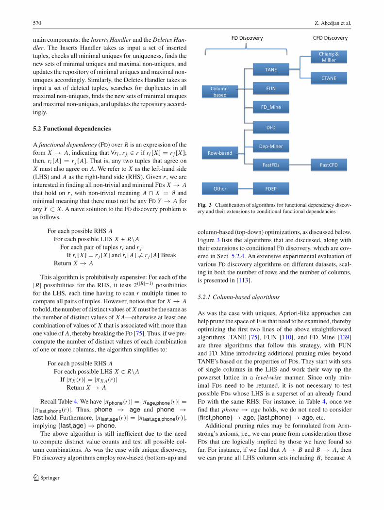
column-based (top-down) optimizations, as discussed below.Figure 3 lists the algorithms that are discussed, along withtheir extensions to conditional Fd discovery, which are cov-ered in Sect. 5.2.4. An extensive experimental evaluation ofvarious Fd discovery algorithms on different datasets, scal-ing in both the number of rows and the number of columns,is presented in [113].
5.2.1 Column-based algorithms
As was the case with uniques, Apriori-like approaches canhelp prune the space of Fds that need to be examined, therebyoptimizing the first two lines of the above straightforwardalgorithms. TANE [75], FUN [110], and FD_Mine [139]are three algorithms that follow this strategy, with FUNand FD_Mine introducing additional pruning rules beyondTANE’s based on the properties of Fds. They start with setsof single columns in the LHS and work their way up thepowerset lattice in a level-wise manner. Since only min-imal Fds need to be returned, it is not necessary to testpossible Fds whose LHS is a superset of an already foundFd with the same RHS. For instance, in Table 4, once wefind that phone → age holds, we do not need to consider{first,phone} → age, {last,phone} → age, etc.
Additional pruning rules may be formulated from Arm-strong’s axioms, i.e., we can prune from consideration thoseFds that are logically implied by those we have found sofar. For instance, if we find that A → B and B → A, thenwe can prune all LHS column sets including B, because A
123

Profiling relational data: a survey 571
and B are equivalent [139]. Another pruning strategy is toignore columns sets that have the same number of distinctvalues as their subsets [110]. Returning to Table 4, observethat phone → first does not hold. Since |πphone(r)| =|πlast,phone(r)| = |πage,phone(r)| = |πlast,age,phone(r)|, weknow that adding last and/or age to the LHS cannot lead to avalid Fd with first on the RHS. To determine these cardinal-ities the approaches use a so-called partition data structure,which is similar to the PLIs of Sect. 5.1.3.
5.2.2 Row-based algorithms
Row-based algorithms examine pairs of tuples to determineLHS candidates. Dep-Miner [95] and FastFDs [136] are twoexamples; the FDEP algorithm [52] is also row-based, butthe way it ultimately finds Fds that hold is different.
The idea behind row-based algorithms is to compute theso-called difference sets for each pair of tuples, which arethe columns on which the two tuples differ. Table 5 enu-merates the difference sets in the data from Table 4. Next,we can find candidate LHS’s from the difference sets as fol-lows. Pick a candidate RHS, say, phone. The difference setsthat include phone, with phone removed are as follows:{first,last,age}, {first,age}, {age}, {last} and {first,last}.This means that there exist pairs of tuples with different val-ues of phone and also with different values of these fivedifference sets. Next, we find minimal subsets of columnsthat have a non-empty intersection with each of these differ-ence sets. Such subsets are exactly the LHS’s of minimal Fdswith phone as the RHS: If two tuples have different valuesof phone, they are guaranteed to have different values of thecolumns in the above minimal subsets, and therefore, theydo not cause Fd violations. Here, there is only one such min-imal subset, {last,age}, giving {last,age} → phone. If werepeat this process for each possible RHS, and compute min-imal subsets corresponding to the LHS’s, we obtain the setof minimal Fds. The main difference among row-based Fddiscovery algorithms is in how they find the minimal subsets.
A recent approach to Fd discovery is DFD, which adaptsthe column-based and row-based pruning of the unique dis-covery approach Ducc to the problem of Fd discovery [6].
Table 5 Difference sets computed from Table 4
Tuple ID pair Difference set
(1,2) first, last, age, phone
(1,3) first, age, phone
(1,4) age, phone
(2,3) last, phone
(2,4) first, last, phone
(3,4) first
DFD decomposes the attribute lattice into |R| lattices, con-sidering each attribute as a possible RHS of an Fd. For theremaining |R| − 1 attributes, DFD applies a random walkapproach by pruning supersets of Fd LHS’s and subsets ofnon-Fd LHS’s.
DFD has been experimentally compared to TANE, whichis a column-based approach, and FastFDs, which is row-based [6]. The experiments confirm that row-based approa-ches work well on high-dimensional tables with a relativelysmall number of tuples, while column-based approaches,such as TANE, perform better on low-dimensional tableswith a large number of rows. DFD, which benefits fromrow-based and column-based pruning, performs significantlybetter than TANE and FastFDs, unless the table has verymany tuples and very few columns or vice versa.
5.2.3 Partial and approximate functional dependencies
While Fds were meant for schema design and were enforcedby the database management system, there are many instan-ces inwhich a databasemay not satisfy some Fds exactly. Forexample, the application semantics may have changed overtime and Fd enforcement was disabled, or the database mayhave been created by integrating conflicting data sources. Asa result, it is useful to discover partial or soft Fds, i.e., thosewhich “almost hold,” perhaps with a few exceptions.
A common definition of “almost holding” or “confidence”is the relative size of the largest subset of r on which a givenFd holds exactly divided by |r | [58,85]. For example, if weremove tuple 1 from Table 4, the Fd last → phone holdsexactly, and therefore, its confidence is 3
4 . The CORDS sys-tem for finding soft Fds uses a slightly different definition:The confidence of X → A is |πX (r)|
|πX A(r)| [76]. Other definitionsinvolve computing the number of tuples or tuple pairs that donot violate the Fd divided by |r | or |r |2, respectively [85].
A related notion is that of approximate Fd inference, inwhich partial or exact Fds are generated from a sample ofa relation [76,85]. Of course, even if an Fd holds exactlyon a subset of a relation, it may hold partially on the wholerelation. Approximate Fd inference is appealing from a com-putational standpoint as it requires only a sample of the data.
5.2.4 Conditional functional dependencies
Conditional functional dependencies (Cfds), proposed in[46], encode Fds that hold only on well-defined subsets ofr . For instance, {first,last} → age does not hold on theentire relation in Table 4, but it does hold on a subset of itwhere first = Eve. Formally, a Cfd consists of two parts:an embedded Fd X → A and an accompanying patterntuple with attributes X A. Each cell of a pattern tuple con-tains a value from the corresponding attribute’s domain or awildcard symbol “_”. A pattern tuple identifies a subset of a
123
572 Z. Abedjan et al.
relation instance in a natural way: A tuple ri matches a pat-tern tuple if it agrees on all of its non-wildcard attributes. Inthe above example, we can formulate a Cfd with an embed-ded Fd {first,last} → age and a pattern tuple (Eve, _, _),meaning that the embedded Fd holds only on tuples whichmatch the pattern, i.e., those with first = Eve. We define thesupport of a pattern tuple as the fraction of tuples in r that itmatches; for example, the support of (Eve, _, _) in Table 4is 2
4 .An important special case occurs when the pattern tuple
has no wildcards. For example, the following (admittedlyaccidental) Cfd holds on Table 4: age → phone with apattern tuple (32, 1234). In other words, if age = 32,then phone = 1234. These special cases, which resembleinstance-level association rules (that have 100% confidence),are referred to as constant Cfds.
Additionally, as was the case with traditional Fds, we candefine approximate Cfds as those that hold on the subsetspecified by the pattern tableauwith some exceptions. For thecase of confidence defined as the minimum number of tuplesthat must be removed to make the Cfd hold, [32] gives algo-rithms for computing summaries that allow the confidenceof a Cfd to be estimated with guaranteed accuracy.
Cfd discovery involves a larger search space than Fd dis-covery: In addition to detecting embedded Fds, we mustalso find the pattern tuples. Cfd discovery algorithms typi-cally extend existing Fd discovery algorithms: For example,CTANE [47] and the algorithm from [24] extend TANE,while FastCFD [47] extends FastFDs (see Fig. 3).
Additionally, two simpler problems have been studied.The first is to discover pattern tuples given an embeddedFd [59]. The output of this technique is an (approximately)smallest set of pattern tuples, each leading to an approximateCfdwith a confidence exceeding a user-supplied confidencethreshold, the union of which has a support that exceeds auser-supplied support threshold. The second problem is toreport only the constant Cfds. For this problem, CFDMinerhas been proposed Cfds [47], which is based on frequentitemset mining, as well as FACD [91], which includes morepruning rules. Also, CFUN, an extension of FUN to gen-erating frequent constant Cfds that exceed a given supportthreshold, has been proposed in [42].
5.3 Inclusion dependencies
An inclusion dependency (Ind) between column A of relationR and column B of relation S, written R.A ⊆ S.B, or A ⊆ Bwhen the relations are clear from context, asserts that eachvalue of A appears in B. Similarly, for two sets of columns Xand Y , we write R.X ⊆ S.Y , or X ⊆ Y , when each distinctcombinations of values in X appears in Y . We refer to R.A orR.X as the left-hand side (LHS) and S.B or S.Y as the right-hand side (RHS). Inds with a single-column LHS and RHS
are referred to as unary and those with multiple columns inthe LHS and RHS are called n-ary.
A naive solution to Ind discovery in relation instances rand s is to try to match each possible LHS with each possibleRHS, as shown below.
For each column combination X in RFor each column combination Y in Swith |Y | = |X |If ∀x ∈ πX (r) ∃y ∈ πY (s) such that x = y
Return X ⊆ Y
Note that for any considered X and Y , we can stop as soonaswe find a value combination of X that does not appear inY .Still, this is not an efficient approach as it repeatedly scans rand s when testing the possible LHS and RHS combinations.
5.3.1 Generating unary inclusion dependencies
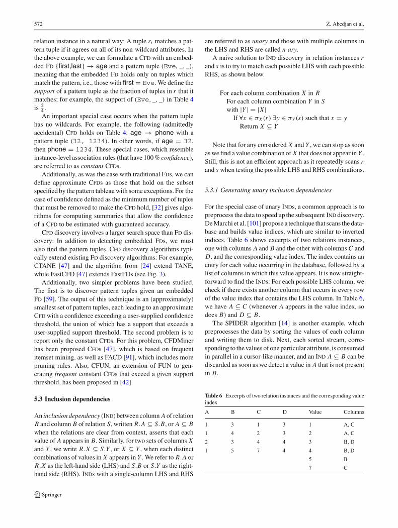
For the special case of unary Inds, a common approach is topreprocess the data to speed up the subsequent Ind discovery.DeMarchi et al. [101] propose a technique that scans the data-base and builds value indices, which are similar to invertedindices. Table 6 shows excerpts of two relations instances,one with columns A and B and the other with columnsC andD, and the corresponding value index. The index contains anentry for each value occurring in the database, followed by alist of columns in which this value appears. It is now straight-forward to find the Inds: For each possible LHS column, wecheck if there exists another column that occurs in every rowof the value index that contains the LHS column. In Table 6,we have A ⊆ C (whenever A appears in the value index, sodoes B) and D ⊆ B.
The SPIDER algorithm [14] is another example, whichpreprocesses the data by sorting the values of each columnand writing them to disk. Next, each sorted stream, corre-sponding to the values of one particular attribute, is consumedin parallel in a cursor-like manner, and an Ind A ⊆ B can bediscarded as soon as we detect a value in A that is not presentin B.
Table 6 Excerpts of two relation instances and the corresponding valueindex
A B C D Value Columns
1 3 1 3 1 A, C
1 4 2 3 2 A, C
2 3 4 4 3 B, D
1 5 7 4 4 B, D
5 B
7 C
123
Profiling relational data: a survey 573
5.3.2 Generating n-ary inclusion dependencies
Once all unary Inds have been discovered, De Marchi etal. [101] give a level-wise algorithm, similar to the TANEalgorithm for Fd discovery, which constructs Inds with icolumns from those with i −1 columns and prunes Inds thatcannot be true. Additionally, hybrid algorithms have beenproposed in [87,102] that combine bottom-up and top-downtraversal for additional pruning.
The Binder algorithm uses divide and conquer principlesto handle larger datasets than relatedwork [114]. In the dividestep, it splits the input dataset horizontally into partitions andvertically into buckets with the goal to fit each partition intomain memory. In the conquer step,Binder then validates theset of all possible inclusion dependency candidates, whichare created in the same fashion as in [101], against the par-titions. Processing one partition after another, the validationconstructs two indexes on each partition, a dense index andan inverted index, and uses them to efficiently prune invalidcandidates from the result set.
5.3.3 Partial and approximate inclusion dependencies
Similar to partial Fds, partial Inds have been defined as thosethat almost hold. Using the notion of removing the fewesttuples so that the remainder satisfies the Ind exactly, we candefine the strength or confidence of a partial Ind X ⊆ Yas |πX (r)|−|πX (r)/πY (r)|
|πX (r)| [96,101]. That is, the confidence isthe number of distinct values of X that appear in Y dividedby the number of distinct values of X . An equivalent bag-semantics version of this definition is to divide the numberof tuples whose X -values appear in Y by the total numberof tuples [61]. According to both definitions, the confidenceof B ⊆ D in Table 6 is 3
4 . Most of the algorithms discussedabove can be extended to discover partial Inds.
5.3.4 Conditional inclusion dependencies
Similar toCfds, conditional inclusion dependencies (Cinds)represent Inds that hold only on well-defined subsets ofrelations [19]. A Cind consists of an embedded standardInd R.X ⊆ S.Y and an accompanying pattern tuple withattributes R.X p and S.Yp ,where X∩X p = ∅ andY∩Yp = ∅.ACind specifies that for the subset of R that matches the X p-values of the pattern tuple, all the X -values must appear inY , and furthermore, the Yp values of these tuples in S mustmatch the Yp-values of the pattern tuple.
For example, suppose a business maintains a Customerstable, keyed by cid, and including a column class indicatingthe class of the customer (e.g., gold or silver). Further-more, suppose a Services table maintains the services thatcustomers subscribe to, including a service id (sid), a cidand the type of service (e.g., hardware or software). Let
Services.cid ⊆ Customers.cid be the embedded Ind andlet (Services.type = software, Customers.class =gold) be a pattern tuple. ThisCind asserts that the customerids in the Services table must be drawn from the customerids in the Customers table, andmoreover, gold customers canobtain only software services. On the other hand, a patterntuple Services.type = software implies that only thesoftware services must have customer ids drawn from thosein the Customers table (e.g., perhaps hardware services areprovided to customers stored in a different table).
Given an embedded Ind, the algorithm from [61], whichalso applies to Cfds, finds pattern tuples that lead to partialCinds with a confidence satisfying a user-supplied threshold.Similarly, Bauckmann et al. [13] start with a set of approx-imate Inds and find pattern tuples to turn these into Cinds;however, in contrast to [61], they are not constrained to asingle embedded Ind. The authors present two algorithms:CINDERELLA, which is based on the Apriori algorithm forassociation rule mining and employs a breadth-first traversalof the powerset lattice, and PLI, which employs a depth-firsttraversal instead.
5.3.5 Generating foreign keys
Ind discovery is a precursor to foreign key detection: Aforeign key must satisfy the corresponding inclusion depen-dency but not all Inds are foreign keys. For example,multipletables may contain auto-increment columns that serve as sur-rogate keys, and while inclusion dependencies among themmay exist, they are not foreign keys. Once Inds have beendiscovered, additional heuristics have been proposed, whichessentially rank the discovered Inds according to their like-lihood of being foreign keys [96,123,143]. A very simplerule may be that if the LHS and RHS have similar names,then A may be a foreign key. It is also useful to examine theset of discovered Inds as a whole: For instance, foreign keysusually are not also primary keys that serve as foreign keysfor other tables, and furthermore, a primary key is often ref-erenced by multiple foreign keys in multiple tables, meaningthat a primary key should appear in theRHSofmultiple Inds,with the LHS’s being the foreign keys. More complex rulesmay reference value distributions; for example, the values ina foreign key column should form a random sample of thevalues in the corresponding primary key column.
5.4 Other dependencies
Having outlined the algorithms for discovering traditionaldependencies and their extensions, we now discuss othertypes of dependencies related to data profiling. Recently, anextension of FastFDs called FastDC was proposed for dis-covering denial constraints, which are universally quantified
123
574 Z. Abedjan et al.
first-order logic formulas that subsume Fds, Cfds, Inds andmany others [29].
Also, functional dependencies have recently been gener-alized to differential dependencies in [128]. A differentialdependency X → Y states that if two tuples have “close”values of X (say, the edit distance between them is small),then their A values must also be close.4 For example, ina financial database, it may be true that if two tuples havesimilar values of date (e.g., within seven days), then theirprice values must also be similar (e.g., within 100 dollars).Row- and column-based approaches to discovering differen-tial dependencies were given in [128].
Another interesting class of dependencies involve order.For instance, it may be useful to discover that if r is sortedon some attribute A, it is also sorted on B, which gives anorder dependency between A and B [56]. This concept wasgeneralized in [57], which proposed sequential dependencies(SDs). An SD states that when sorted on A, any two consec-utive values of B must be within a predefined range. Givena complete SD, including the attributes A and B as well asthe range, [57] gives an algorithm for discovering ranges ofvalues of A in which the SD is approximately satisfied. To thebest of our knowledge, the general problem of SD discoveryfrom data is open.
5.5 Summary and discussion
Dependency discovery has been a popular research area indatamanagement.Many of the algorithms and techniques fordependency discovery are based upon classical data miningsolutions, such as the Apriori algorithm for efficient gener-ation of association rules. Additional technical challengesarise in the context of conditional dependencies, and novelsearch space pruning strategies have been developed basedon the properties of the given dependencies.
Data profiling results can be not only complex, but alsovery large. For instance, it is not uncommon to find thousandsof functional dependencies in a given dataset. To handle thisand focus users on themost important, interesting, or surpris-ing ones, ranking profiling results can help, as Chu et al. [29]show for denial constraints. They suggest two functions,namely succinctness and coverage, to assess their interest-ingness. Similar interestingness functions for Cfds are givenby Chiang and Miller [24]. Additionally, Andritsos et al. [9]show how to rank Fds according to their information con-tent. Furthermore, as we discussed earlier, post-processingmethods have been proposed to determine which of the dis-covered inclusion dependencies are likely to be foreign keys;
4 Differential dependencies also generalize matching dependencies[49] (if two tuples have close values of X , their A valuesmust be exactlythe same) and metric functional dependencies [89] (if two tuples havethe same values of X , their A values must be close).
however, we are not aware of corresponding techniques foruniques and Fds.
6 Profiling tools
Whenever data are too voluminous to fit on a screen or a sheetof paper, data profiling is performed. Even lacking explicitprofiling tools, much can already be done with data man-agement tools, such as spreadsheet software, SQL queries,search capabilities of text editors or simply by “eyeballing”the data. Such methods to become acquainted with a newset of data are probably familiar to most readers. The simplemethod of sorting the values of a column can already revealminimum and maximum values, and scrolling through thatsorted data intuits the value distribution, including the num-ber of null values, which are typically sorted to the verybeginning or end, and the uniqueness of a column. Findingthemedian or average values requires additional calculations,whereas it is infeasible to detect dependencies with such sim-ple means.
To allow a more powerful and integrated approach to dataprofiling, software companies have developed data profilingtools, mostly to profile data residing in relational databases.Most tools discussed in this survey are part of a larger soft-ware suite, either for data integration or for data cleansing.We first give an overview of tools that were created in thecontext of a research project (see Table 7 for a listing). Then,we give a brief glimpse of the vast set of commercial toolswith profiling capabilities (see Table 8 for a listing).
6.1 Research tools
In the research literature, data profiling tools are often embed-ded in data cleaning systems. For example, the Bellman [38]data quality browser supports column analysis (counting thenumber of rows, distinct values, and NULL values, findingthe most frequently occurring values, etc.), and key detection(up to four columns). It also provides a column similar-ity functionality that finds columns whose value or n-gramdistributions are similar; this is helpful for discovering poten-tial foreign keys and join paths. Furthermore, an interestingapplication of Bellman was to profile the evolution of a data-base using value distributions and correlations [37]: Whichtables change over time and in what ways (insertions, dele-tions, modifications), and which groups of tables tend tochange in the same way. The Potters Wheel tool [122] alsosupports column analysis, in particular, detecting data typesand syntactic structures/patterns.
Data profiling functionality is also included in theMADLib toolkit for scalable in-database analytics [71],including column statistics, such as count, count distinct,
123
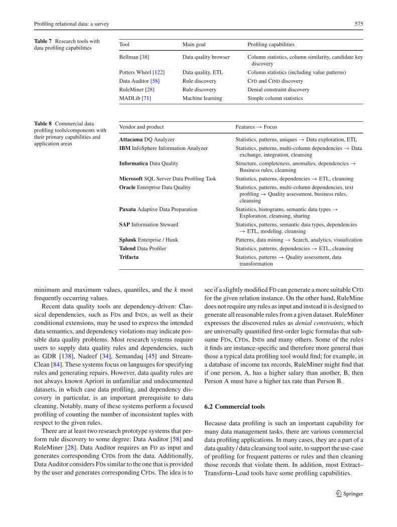
Profiling relational data: a survey 575
Table 7 Research tools withdata profiling capabilities
Tool Main goal Profiling capabilities
Bellman [38] Data quality browser Column statistics, column similarity, candidate keydiscovery
Potters Wheel [122] Data quality, ETL Column statistics (including value patterns)
Data Auditor [58] Rule discovery Cfd and Cind discovery
RuleMiner [28] Rule discovery Denial constraint discovery
MADLib [71] Machine learning Simple column statistics
Table 8 Commercial dataprofiling tools/components withtheir primary capabilities andapplication areas
Vendor and product Features → Focus
Attacama DQ Analyzer Statistics, patterns, uniques → Data exploration, ETL
IBM InfoSphere Information Analyzer Statistics, patterns, multi-column dependencies → Dataexchange, integration, cleansing
Informatica Data Quality Structure, completeness, anomalies, dependencies →Business rules, cleansing
Microsoft SQL Server Data Profiling Task Statistics, patterns, dependencies → ETL, cleansing
Oracle Enterprise Data Quality Statistics, patterns, multi-column dependencies, textprofiling → Quality assessment, business rules,cleansing
Paxata Adaptive Data Preparation Statistics, histograms, semantic data types →Exploration, cleansing, sharing
SAP Information Steward Statistics, patterns, semantic data types, dependencies→ ETL, modeling, cleansing
Splunk Enterprise / Hunk Patterns, data mining → Search, analytics, visualization
Talend Data Profiler Statistics, patterns, dependencies → ETL, cleansing
Trifacta Statistics, patterns → Quality assessment, datatransformation
minimum and maximum values, quantiles, and the k mostfrequently occurring values.
Recent data quality tools are dependency-driven: Clas-sical dependencies, such as Fds and Inds, as well as theirconditional extensions, may be used to express the intendeddata semantics, and dependency violations may indicate pos-sible data quality problems. Most research systems requireusers to supply data quality rules and dependencies, suchas GDR [138], Nadeef [34], Semandaq [45] and Stream-Clean [84]. These systems focus on languages for specifyingrules and generating repairs. However, data quality rules arenot always known Apriori in unfamiliar and undocumenteddatasets, in which case data profiling, and dependency dis-covery in particular, is an important prerequisite to datacleaning. Notably, many of these systems perform a focusedprofiling of counting the number of inconsistent tuples withrespect to the given rules.
There are at least two research prototype systems that per-form rule discovery to some degree: Data Auditor [58] andRuleMiner [28]. Data Auditor requires an Fd as input andgenerates corresponding Cfds from the data. Additionally,DataAuditor considers Fds similar to the one that is providedby the user and generates corresponding Cfds. The idea is to
see if a slightlymodified Fd can generate amore suitableCfdfor the given relation instance. On the other hand, RuleMinedoes not require any rules as input and instead it is designed togenerate all reasonable rules from a given dataset. RuleMinerexpresses the discovered rules as denial constraints, whichare universally quantified first-order logic formulas that sub-sume Fds, Cfds, Inds and many others. Some of the rulesit finds are instance-specific and therefore more general thanthose a typical data profiling tool would find; for example, ina database of income tax records, RuleMiner might find thatif one person, A, has a higher salary than another, B, thenPerson A must have a higher tax rate than Person B.
6.2 Commercial tools
Because data profiling is such an important capability formany data management tasks, there are various commercialdata profiling applications. In many cases, they are a part of adata quality / data cleansing tool suite, to support the use-caseof profiling for frequent patterns or rules and then cleaningthose records that violate them. In addition, most Extract–Transform–Load tools have some profiling capabilities.
123

576 Z. Abedjan et al.
Table 8 mentions prominent examples of current com-mercial tools, together with their capabilities and applicationfocus, based on the respective product documentations. It isbeyond the scope of this survey to provide a market overviewor compile featurematrices.We also deliberately refrain fromproviding staticURLs for the various products, because com-mercial Web sites are too fickle.
Finally, and as mentioned before, every database man-agement system collects and maintains base statistics aboutthe tables it manages. However, they do not readily exposethose metadata, the metadata are not always up-to-date andsometimes based only on samples, and their scope is usuallylimited to simple counts and cardinalities.
7 Next generation profiling
Recent trends in data management have added new chal-lenges but also opportunities for data profiling. First, underthe big data umbrella, industry and research have turned theirattention to data that they do not own or have not made useof yet. Data profiling can help assess which data might beuseful and reveals the yet unknown characteristics of suchnew data. Second, much of the data that shall be exploited isof non-traditional type for data profiling, i.e., non-relational,non-structured (textual), and heterogeneous. And it is oftentruly “big,” both in terms of schema and in terms of data.Many existing profiling methods cannot adequately handlethat kind of data: Either they do not scalewell, or there simplyare no methods yet. Third, different and new data manage-ment architectures and frameworks have emerged, includingdistributed systems, key-value stores, multi-core- or main-memory-based servers, column-oriented layouts, streaminginput, etc. We discuss some of these trends and their impli-cations toward data profiling. A more elaborate overview ofupcoming challenges of data profiling is in [108].
7.1 Profiling for integration
An important use-case of traditional data profilingmethods isdata integration. Knowledge about the properties of differentdata sources is important to create correct schema mappingsand data transformations, and to correctly standardize andcleanse the data. For instance, knowledge of inclusion depen-denciesmight hint uponways to join two yet unrelated tables.
However, data profiling can reach beyond such support-ive tasks and assess the integrability or ease of integrationof datasets and thus also indicate the necessary integrationeffort, which is vital to project planning. Integration effortmight be expressed in terms of similarity, but also in termsof manmonths or in terms of which tools are needed.
Like integration projects themselves, integrability has twodimensions, namely schematic fit and data fit. Schematic fit is
the degree to which two schemata complement and overlapeach other and can be determined using schema matchingtechniques [44]. Smith et al. [127] have recognized thatschema matching techniques often play the role of profilingtools: Rather than using them to derive schema mappingsand perform data transformation, they might assess projectfeasibility. Finally, the mere matching of schema elementsmight not suffice as a profiling-for-integration result: Addi-tional column metadata can provide further details about theintegration difficulty.
Data fit is the (estimated) number of real-world objectsthat are represented in both datasets, or that are representedmultiple times in a single dataset and how different theyare. Such multiple representations are typically identifiedusing entity matching methods (also known as record link-age, duplicate detection, etc.) [27]. However, estimating thenumber ofmatcheswithout actually performing thematchingon the entire dataset is an open problem.
7.2 Profiling non-relational data
With the rapid growth of the World Wide Web, semi-structured data, such as XML and Rdf data, and non-structured data, such as text document corpora, have becomemore important. Themore flexible structure of non-relationaldatasets opens new challenges for profiling algorithms. Sofar, most methods apply only to or were developed for rela-tional data. Below,we give an overview of both existingworkthat applies traditional profiling algorithms, as well as exist-ing work about data-model-specific profiling approaches, tonon-relational data. We focus on the three most relevant non-relational data formats: XML, Rdf, and text documents.
7.2.1 XML
XML is the quasi-standard for exchanging data on the Web.Many applications, especially Web services, provide theirresults as XML documents. Because the XML structureexplicitly containsmarkup and schema information, differentprofiling approaches have to be considered. Apart from that,Web services themselves are accessible through XML docu-ments, such as WSDL and SOAP files, which are also worthprofiling for Web service inspection and categorization.
There has already been a number of research approachesand proposals with a focus on statistical analysis of XML-formatted data. They concentrate either on theDTDstructure,the XSD schema structure, or the inherent structure of XMLdocuments. The analysis concentrates on gathering statisticsabout the number of root elements, attributes, the depth ofcontent models, etc. [26,105,106,124].
Further approaches focus on algorithms that identify tradi-tional relational dependencies in XML data. While Vincentet al. extend the notion of Fds to XML data [132], Yu et
123

Profiling relational data: a survey 577
al.s [140] present an approach for discovering redundanciesbased on identified XML Fd. There have also been adapta-tions of unique and key discovery concepts and algorithms toXML data [22]. Due to the more relaxed structure of XML,these approaches identify approximate keys [62] or validatethe consistency of the identified keys against XSD defini-tions [10].
As many XML documents do not refer to a specificschema, a relevant application of profiling approaches is tosupport the process of schema extraction [17,69]. Addition-ally, the vast amount of existing documents do not alwayscomply to specified syntactical rules [88], which can be iden-tified via appropriate profiling techniques.
7.2.2 RDF
Although profiling tasks for XML data can easily be adaptedto Rdf datasets and vice versa, the requirement for Rdf datato be machine readable and its important use-case LinkedOpenData (Lod) give rise toRdf-specific challenges for dataprofiling. There are already some tools that generatemetadatafor a given Rdf dataset. For example, LODStats is a stream-based approach for gathering comprehensive statistics aboutRdf datasets [12].
ProLod++ provides additional functionalities by applyingclustering and rule mining techniques [1]. When profilingRdf data, there are many interestingmetadata beyond simplestatistics and patterns of Rdf statement elements, includingsynonymously used properties [4], inverse relationships ofproperties, the conformity and consistence of Rdf structureddata to the corresponding ontology [2], and the distributionof literals and de-referenceable resource Uris from differentnamespaces.
Because of the heterogeneity of interlinked sources, it isvital to identify where specific facts come from and how reli-able they are. Therefore, another interesting task for profilingRdf data is provenance analysis [18].
7.2.3 Text
Many text analysis approaches and applications can beregarded as text profiling tasks. Statistical methods are usedfor tasks, such as information extraction [125], part-of-speech tagging [20], and text categorization [83].
Specifically, in the field of author attribution, there hasbeen research on defining interesting features, such as word-length distributions, average number of syllables [73].
Additionally, linguistic metrics, such as distinctiveness,type-token ratio, and Simpson’s index have been proposedto measure the style and diversity of text documents. Thetask of profiling can target single documents, such as apaper or a book, as well as sets of documents, such asWeb document corpora, product reviews, or user comments.
More sophisticated applications that use metadata gener-ated through profiling include sentiment analysis and opinionmining [93,112].
7.3 Profiling dynamic data
Data profiling describes an instance of a dataset at a particulartime. Since many applications work on frequently changingdata, it is desirable to re-profile a dataset after a change,such as a deletion, insertion, or update, in order to obtainup-to-date metadata. Simple aggregates are easy to main-tain incrementally, but many statistics needed for columnanalysis, such as distinct value counts, cannot be maintainedexactly using limited space and time. For these aggregates,stream sketching techniques [53] may be used to maintainapproximate answers. There are also techniques for con-tinuously updating discovered association rules [131] andclusters [43].
Dependency detection may be too time-consuming forrepeated execution on the entire dataset. Thus, it is necessaryto incrementally update the metadata without processing thecomplete dataset again. One example is Swan, an approachfor unique discovery on dynamic datasets with insertionsand deletions [5] as reported in Sect. 5.1.4. Also, Wang etal. present an approach for maintaining discovered Fds afterdata deletions [134]. From a data cleaning standpoint, thereare solutions for incremental detection of Fd and Cfd vio-lations [50], and incremental data repairing with respect toFds andCfds [30]. In general, incremental solutions for Fds,Cfds, Inds, and Cinds on growing and changing datasetsremain challenges for future research.
7.4 Profiling on new architectures
There are at least two database architecture trends thataffect profiling. The first is column versus row storage.Column-store systems appear to have a natural computa-tional advantage, at least in terms of the column analysistasks we discussed in Sect. 3, since they can directly fetchthe column of interest and compute statistics on it. How-ever, if all columns are to be profiled, the entire dataset mustbe read and the only remaining advantage of column storesmay be their potential compression. The second trend is thatof distributed and cloud data management. This introducesadditional profiling challenges, such as combining statisticsfrom multiple nodes into final per-column analysis. Therehas been some work on detecting Fd and Cfd violations in adistributed database [48,50], but many other problems in thisspace, such as efficient dependency detection in distributeddata, remain open.
123

578 Z. Abedjan et al.
7.5 Visualization
Because data profiling mostly targets human users, effec-tively visualizing any profiling results is of utmost impor-tance. Only then can users interpret results and react to them.A suggestion for a visual data profiling tool is the Profilersystem by Kandel et al. [81]. A strong cooperation betweenthe database community, which produces the data and meta-data to be visualized, and the visualization community,whichenables users to understand and make use of the data, isneeded.
8 Summary
In this article, we provided a comprehensive survey of thestate of the art in data profiling: the set of activities andprocesses to determine metadata about a given database. Wediscussed single-column profiling tasks such as identifyingdata types, value distributions andpatterns, andmulti-columntasks such as detecting various kinds of dependencies. Asthe amount of data and users who require access to dataincrease, efficient and effective data profilingwill continue tobe an important data management problem in research andpractice. While many data profiling algorithms have beenproposed and implemented in research prototypes and com-mercial tools, furtherwork is needed, especially in the contextof profiling new types of data, supporting and leveraging newdata management architectures, and interpreting and visual-izing data profiling results.
References
1. Abedjan, Z., Grütze, T., Jentzsch, A., Naumann, F.: Mining andprofiling RDF data with ProLOD++. In: Proceedings of the Inter-national Conference onData Engineering (ICDE), pp. 1198–1201(2014). Demo
2. Abedjan, Z., Lorey, J., Naumann, F.: Reconciling ontologies andthe web of data. In: Proceedings of the International Conferenceon Information and Knowledge Management (CIKM), pp. 1532–1536 (2012)
3. Abedjan, Z., Naumann, F.: Advancing the discovery of uniquecolumn combinations. In: Proceedings of the International Con-ference on Information and Knowledge Management (CIKM),pp. 1565–1570 (2011)
4. Abedjan, Z., Naumann, F.: Synonym analysis for predicate expan-sion. In: Proceedings of the Extended Semantic Web Conference(ESWC), pp. 140–154 (2013)
5. Abedjan, Z., Quiané-Ruiz, J.-A., Naumann, F.: Detecting uniquecolumn combinations on dynamic data. In: Proceedings of theInternational Conference on Data Engineering (ICDE), pp. 1036–1047 (2014)
6. Abedjan, Z., Schulze, P., Naumann, F.: DFD: efficient functionaldependency discovery. In: Proceedings of the International Con-ference on Information and Knowledge Management (CIKM),pp. 949–958 (2014)
7. Agrawal, D., Bernstein, P., Bertino, E., Davidson, S., Dayal,U., Franklin, M., Gehrke, J., Haas, L., Halevy, A., Han, J.,Jagadish, H.V., Labrinidis, A., Madden, S., Papakonstantinou, Y.,Patel, J.M., Ramakrishnan, R., Ross, K., Shahabi, C., Suciu, D.,Vaithyanathan, S., Widom, J.: Challenges and opportunities withBig Data. Technical report, Computing Community Consortium.http://cra.org/ccc/docs/init/bigdatawhitepaper.pdf (2012)
8. Agrawal, R., Srikant, R.: Fast algorithms for mining associationrules in large databases. In: Proceedings of the International Con-ference on Very Large Databases (VLDB), pp. 487–499 (1994)
9. Andritsos, P., Miller, R.J., Tsaparas, P.: Information-theoretictools for mining database structure from large data sets. In: Pro-ceedings of the International Conference onManagement of Data(SIGMOD), pp. 731–742 (2004)
10. Arenas, M., Daenen, J., Neven, F., Ugarte, M., Van den Bussche,J., Vansummeren, S.: Discovering XSD keys from XML data. In:Proceedings of the International Conference on Management ofData (SIGMOD), pp. 61–72 (2013)
11. Astrahan,M.M., Schkolnick,M.,Kyu-Young,W.:Approximatingthe number of unique values of an attribute without sorting. Inf.Syst. 12(1), 11–15 (1987)
12. Auer, S., Demter, J., Martin, M., Lehmann, J.: LODStats—anextensible framework for high-performance dataset analytics. In:Proceedings of the International Conference on Knowledge Engi-neering and Knowledge Management (EKAW), pp. 353–362(2012)
13. Bauckmann, J., Abedjan, Z., Müller, H., Leser, U., Naumann, F.:Discovering conditional inclusion dependencies. In: Proceedingsof the International Conference on Information and KnowledgeManagement (CIKM), pp. 2094–2098 (2012)
14. Bauckmann, J., Leser, U., Naumann, F., Tietz, V.: Efficientlydetecting inclusion dependencies. In: Proceedings of the Interna-tional Conference on Data Engineering (ICDE), pp. 1448–1450(2007)
15. Benford, F.: The law of anomalous numbers. Proc. Am. Philos.Soc. 78(4), 551–572 (1938)
16. Berti-Equille, L., Dasu, T., Srivastava, D.: Discovery of complexglitch patterns: a novel approach to quantitative data cleaning. In:Proceedings of the International Conference on Data Engineering(ICDE), pp. 733–744 (2011)
17. Bex, G.J., Neven, F., Vansummeren, S.: Inferring XML schemadefinitions from XML data. In: Proceedings of the InternationalConference on Very Large Databases (VLDB), pp. 998–1009(2007)
18. Böhm, C., Lorey, J., Naumann, F.: Creating void descriptions forweb-scale data. J. Web Semant. 9(3), 339–345 (2011)
19. Bravo, L., Fan, W., Ma, S.: Extending dependencies with con-ditions. In: Proceedings of the International Conference on VeryLarge Databases (VLDB), pp. 243–254 (2007)
20. Brill, E.: Transformation-based error-driven learning and naturallanguage processing: a case study in part-of-speech tagging. Com-put. Linguist. 21(4), 543–565 (1995)
21. Brin, S., Motwani, R., Silverstein, C.: Beyond market baskets:generalizing association rules to correlations. SIGMOD Rec.26(2), 265–276 (1997)
22. Buneman, P., Davidson, S.B., Fan,W.,Hara, C.S., Tan,W.C.: Rea-soning about keys for XML. Inf. Syst. 28(8), 1037–1063 (2003)
23. Chandola, V., Kumar, V.: Summarization—compressing data intoan informative representation. Knowl. Inf. Syst. 12(3), 355–378(2007)
24. Chiang, F., Miller, R.J.: Discovering data quality rules. Proc.VLDB Endow. 1, 1166–1177 (2008)
25. Chiang, R.H.L., Cecil, C.E.H., Lim, E.-P.: Linear correlation dis-covery in databases: a data mining approach. Data Knowl. Eng.53(3), 311–337 (2005)
123
Profiling relational data: a survey 579
26. Choi, B.: What are real DTDs like? In: Proceedings of the ACMSIGMOD Workshop on the Web and Databases (WebDB), pp.43–48 (2002)
27. Christen, P.: Data Matching. Springer, Berlin (2012)28. Chu, X., Ilyas, I., Papotti, P., Ye, Y.: RuleMiner: data quality
rules discovery. In: Proceedings of the International Conferenceon Data Engineering (ICDE), pp. 1222–1225 (2014)
29. Chu, X., Ilyas, I.F., Papotti, P.: Discovering denial constraints.Proc. VLDB Endow. 6(13), 1498–1509 (2013)
30. Cong, G., Fan, W., Geerts, F., Jia, X., Ma, S.: Improving dataquality: consistency and accuracy. In: Proceedings of the Interna-tional Conference onVeryLargeDatabases (VLDB), pp. 315–326(2007)
31. Cormode, G., Garofalakis, M., Haas, P.J., Jermaine, C.: Synopsesfor massive data: samples, histograms, wavelets, sketches. Found.Trends Databases 4(13), 1–294 (2011)
32. Cormode, G., Golab, L., Flip, K., McGregor, A., Srivastava, D.,Zhang, X.: Estimating the confidence of conditional functionaldependencies. In: Proceedings of the International Conference onManagement of Data (SIGMOD), pp. 469–482 (2009)
33. Cormode, G., Korn, F., Muthukrishnan, S., Srivastava, D.: Space-and time-efficient deterministic algorithms for biased quantilesover data streams. In: Proceedings of theSymposiumonPrinciplesof Database Systems (PODS), pp. 263–272 (2006)
34. Dallachiesa, M., Ebaid, A., Eldawy, A., Elmagarmid, A., Ilyas,I.F., Ouzzani, M., Tang, N.: NADEEF: a commodity data clean-ing system. In: Proceedings of the International Conference onManagement of Data (SIGMOD), pp. 541–552 (2013)
35. Das, A., Ng, W.-K., Woon, Y.-K.: Rapid association rule mining.In: Proceedings of the International Conference on Informationand Knowledge Management (CIKM), pp. 474–481 (2001)
36. Dasu, T., Johnson, T.: Hunting of the snark: finding data glitchesusing data mining methods. In: Proceedings of the InternationalConference on Information Quality (IQ), pp. 89–98 (1999)
37. Dasu, T., Johnson, T., Marathe, A.: Database explorationusing database dynamics. IEEE Data Eng. Bull. 29(2), 43–59(2006)
38. Dasu, T., Johnson, T.,Muthukrishnan, S., Shkapenyuk,V.:Miningdatabase structure; or, how to build a data quality browser. In:Proceedings of the International Conference on Management ofData (SIGMOD), pp. 240–251 (2002)
39. Dasu, T., Loh, J.M.: Statistical distortion: consequences of datacleaning. Proc. VLDB Endow. 5(11), 1674–1683 (2012)
40. Dasu, T., Loh, J.M., Srivastava, D.: Empirical glitch expla-nations. In: Proceedings of the International Conference onKnowledge Discovery and Data Mining (SIGKDD), pp. 572–581(2014)
41. Deshpande, A., Garofalakis, M., Rastogi, R.: Independenceis good: dependency-based histogram synopses for high-dimensional data. In: Proceedings of the International Conferenceon Management of Data (SIGMOD), pp. 199–210 (2001)
42. Diallo, T., Novelli, N., Petit, J.-M.: Discovering (frequent) con-stant conditional functional dependencies. Int. J. Data Min.Model. Manag. 4(3), 205–223 (2012)
43. Ester, M., Kriegel, H.-P., Sander, J., Wimmer, M., Xu, X.: Incre-mental clustering for mining in a data warehousing environment.In: Proceedings of the International Conference on Very LargeDatabases (VLDB), pp. 323–333 (1998)
44. Euzenat, J., Shvaiko, P.: Ontology Matching, 2nd edn. Springer,Berlin (2013)
45. Fan,W., Geerts, F., Jia, X.: Semandaq: a data quality system basedon conditional functional dependencies. Proc. VLDB Endow.1(2), 1460–1463 (2008)
46. Fan, W., Geerts, F., Jia, X., Kementsietsidis, A.: Conditionalfunctional dependencies for capturing data inconsistencies. ACMTrans. Database Syst. 33(2), 1–48 (2008)
47. Fan, W., Geerts, F., Li, J., Xiong, M.: Discovering conditionalfunctional dependencies. IEEE Trans. Knowl. Data Eng. 23(4),683–698 (2011)
48. Fan, W., Geerts, F., Ma, S., Müller, H.: Detecting inconsistenciesin distributed data. In: Proceedings of the International Confer-ence on Data Engineering (ICDE), pp. 64–75 (2010)
49. Fan, W., Jia, X., Li, J., Ma, S.: Reasoning about record matchingrules. Proc. VLDB Endow. 2(1), 407–418 (2009)
50. Fan, W., Li, J., Tang, N., Yu, W.: Incremental detection of incon-sistencies in distributed data. In: Proceedings of the InternationalConference on Data Engineering (ICDE), pp. 318–329 (2012)
51. Fernau, H.: Algorithms for learning regular expressions from pos-itive data. Inf. Comput. 207(4), 521–541 (2009)
52. Flach, P.A., Savnik, I.:Database dependencydiscovery: amachinelearning approach. AI Commun. 12(3), 139–160 (1999)
53. Ganguly, S.: Counting distinct items over update streams. Theor.Comput. Sci. 378(3), 211–222 (2007)
54. Garofalakis, M., Keren, D., Samoladas, V.: Sketch-based geomet-ric monitoring of distributed stream queries. Proc. VLDB Endow.6(10), 937–948 (2013)
55. Giannella, C., Wyss, C.: Finding minimal keys in a relationinstance (1999). http://citeseerx.ist.psu.edu/viewdoc/summary?doi=?doi=10.1.1.41.7086
56. Ginsburg, S., Hull, R.: Order dependency in the relational model.Theor. Comput. Sci. 26, 149–195 (1983)
57. Golab, L., Karloff, H., Korn, F., Saha, A., Srivastava, D.: Sequen-tial dependencies. Proc. VLDB Endow. 2(1), 574–585 (2009)
58. Golab, L., Karloff, H., Korn, F., Srivastava, D.: Data auditor:exploring data quality and semantics using pattern tableaux. Proc.VLDB Endow. 3(1–2), 1641–1644 (2010)
59. Golab, L., Karloff, H., Korn, F., Srivastava, D., Bei, Y.: On gener-ating near-optimal tableaux for conditional functional dependen-cies. Proc. VLDB Endow. 1(1), 376–390 (2008)
60. Golab, L., Korn, F., Srivastava, D.: Discovering pattern tableauxfor data quality analysis: a case study. In: Proceedings of the Inter-national Workshop on Quality in Databases (QDB), pp. 47–53(2011)
61. Golab, L., Korn, F., Srivastava, D.: Efficient and effective analysisof data quality using pattern tableaux. IEEEData Eng. Bull. 34(3),26–33 (2011)
62. Grahne, G., Zhu, J.: Discovering approximate keys in XML data.In: Proceedings of the International Conference on Informationand Knowledge Management (CIKM), pp. 453–460 (2002)
63. Gray, J., Chaudhuri, S., Bosworth, A., Layman, A., Reichart, D.,Venkatrao, M., Pellow, F., Pirahesh, H.: Data cube: a relationalaggregation operator generalizing group-by, cross-tab, and subtotals. Data Min. Knowl. Discov. 1(1), 29–53 (1997)
64. Gunopulos, D., Khardon, R., Mannila, H., Sharma, R.S.: Discov-ering all most specific sentences. ACM Trans. Database Syst. 28,140–174 (2003)
65. Haas, P.J., Naughton, J.F., Seshadri, S., Stokes, L.: Sampling-based estimation of the number of distinct values of an attribute.In: Proceedings of the International Conference on Very LargeDatabases (VLDB), pp. 311–322 (1995)
66. Hainaut, J.-L., Henrard, J., Englebert, V., Roland, D., Hick, J.-M.: Database reverse engineering. In: Liu, L., Tamer Özsu, M.(eds.) Encyclopedia of Database Systems, pp. 723–728. Springer,Heidelberg (2009)
67. Han, J., Pei, J.,Yin,Y.:Mining frequent patternswithout candidategeneration. SIGMOD Rec. 29(2), 1–12 (2000)
68. Hanrahan, P.: Analytic database technology for a new kind ofuser—the data enthusiast (keynote). In: Proceedings of the Inter-national Conference on Management of Data (SIGMOD), pp.577–578 (2012)
69. Hegewald, J., Naumann, F., Weis, M.: XStruct: efficient schemaextraction from multiple and large XML databases. In: Proceed-
123
580 Z. Abedjan et al.
ings of the International Workshop on Database Interoperability(InterDB) (2006)
70. Heise, A., Quiané-Ruiz, J.-A., Abedjan, Z., Jentzsch, A., Nau-mann, F.: Scalable discovery of unique column combinations.Proc. VLDB Endow. 7(4), 301–312 (2013)
71. Hellerstein, J.M., Ré, C., Schoppmann, F., Wang, D.Z., Fratkin,E., Gorajek, A., Ng, K.S., Welton, C., Feng, X., Li, K., Kumar,A.: The MADlib analytics library or MAD skills, the SQL. Proc.VLDB Endow. 5(12), 1700–1711 (2012)
72. Hipp, J., Güntzer, U., Nakhaeizadeh, G.: Algorithms for associ-ation rule mining—a general survey and comparison. SIGKDDExplor. 2(1), 58–64 (2000)
73. Holmes, D.I.: Authorship attribution. Comput. Humanit. 28, 87–106 (1994)
74. Hua, M., Pei, J.: Cleaning disguised missing data: a heuristicapproach. In: Proceedings of the International Conference onKnowledge Discovery and Data Mining (SIGKDD), pp. 950–958(2007)
75. Huhtala, Y., Kärkkäinen, J., Porkka, P., Toivonen, H.: TANE: anefficient algorithm for discovering functional and approximatedependencies. Comput. J. 42(2), 100–111 (1999)
76. Ilyas, I.F., Markl, V., Haas, P.J., Brown, P., Aboulnaga, A.:CORDS: automatic discovery of correlations and soft functionaldependencies. In: Proceedings of the International Conference onManagement of Data (SIGMOD), pp. 647–658 (2004)
77. Ioannidis, Y.: The history of histograms (abridged). In: Proceed-ings of the International Conference on Very Large Databases(VLDB), pp. 19–30 (2003)
78. Jain, A.K., Narasimha Murty, M., Flynn, P.J.: Data clustering: areview. ACM Comput. Surv. 31(3), 264–323 (1999)
79. Johnson,T.: Encyclopedia ofDatabaseSystems, chapterData Pro-filing. Springer, Heidelberg (2009)
80. Kache,H.,Han,W.-S.,Markl,V., Raman,V., Ewen, S.: POP/FED:progressive query optimization for federated queries in DB2. In:Proceedings of the International Conference on Very Large Data-bases (VLDB), pp. 1175–1178 (2006)
81. Kandel, S., Parikh, R., Paepcke, A., Hellerstein, J., Heer, J.:Profiler: integrated statistical analysis and visualization for dataquality assessment. In: Proceedings ofAdvancedVisual Interfaces(AVI), pp. 547–554 (2012)
82. Kang, J., Naughton, J.F.: On schema matching with opaque col-umn names and data values. In: Proceedings of the InternationalConference on Management of Data (SIGMOD), pp. 205–216(2003)
83. Keim, D.A., Oelke, D.: Literature fingerprinting: a new methodfor visual literary analysis. In: Proceedings of Visual AnalyticsScience and Technology (VAST), pp. 115–122 (2007)
84. Khoussainova, N., Balazinska, M., Suciu, D.: Towards correctinginput data errors probabilistically using integrity constraints. In:Proceedings of the ACM International Workshop on Data Engi-neering for Wireless and Mobile Access (MobiDE), pp. 43–50(2006)
85. Kivinen, J., Mannila, H.: Approximate inference of functionaldependencies from relations. In: Proceedings of the Interna-tional Conference on Database Theory (ICDT), pp. 129–149(1995)
86. Koehler, H., Leck, U., Link, S., Prade, H.: Logical foundations ofpossibilistic keys. In: Fermé, E., Leite, J. (eds.) Logics inArtificialIntelligence, volume 8761 of Lecture Notes in Computer Science,pp. 181–195. Springer, Heidelberg (2014)
87. Koeller, A., Rundensteiner, E.A.: Heuristic strategies for the dis-covery of inclusion dependencies and other patterns. J. DataSemant. V. 3870, 185–210 (2006)
88. Korn, F., Saha, B., Srivastava, D., Ying, S.: On repairing structuralproblems in semi-structured data. Proc. VLDBEndow. 6(9), 601–612 (2013)
89. Koudas, N., Saha, A., Srivastava, D., Venkatasubramanian, S.:Metric functional dependencies. In: Proceedings of the Interna-tional Conference on Data Engineering (ICDE), pp. 1275–1278(2009)
90. Laney,D.: 3Ddatamanagement: controllingdata volume, velocityand variety. Technical report, Gartner (2001)
91. Li, J., Liu, J., Toivonen, H., Yong, J.: Effective pruning for the dis-covery of conditional functional dependencies. Comput. J. 56(3),378–392 (2013)
92. Li, Y., Krishnamurthy, R., Raghavan, S., Vaithyanathan, S.,Jagadish, H.V.: Regular expression learning for informationextraction. In: Proceedings of the Conference on Empirical Meth-ods in Natural Language Processing (EMNLP), pp. 21–30 (2008)
93. Liu, B.: Sentiment analysis and subjectivity. Handbook of NaturalLanguage Processing, 2nd edn. Chapman and Hall/CRC, London(2010)
94. Liu, J., Li, J., Liu, C., Chen, Y.: Discover dependencies fromdata—a review. IEEE Trans. Knowl. Data Eng. 24(2), 251–264(2012)
95. Lopes, S., Petit, J.-M., Lakhal, L.: Efficient discovery of func-tional dependencies and Armstrong relations. In: Proceedings ofthe International Conference on Extending Database Technology(EDBT), pp. 350–364 (2000)
96. Lopes, S., Petit, J.-M., Toumani, F.: Discovering interesting inclu-sion dependencies: application to logical database tuning. Inf.Syst. 27(1), 1–19 (2002)
97. Lucchesi, C.L., Osborn, S.L.: Candidate keys for relations. J.Comput. Syst. Sci. 17(2), 270–279 (1978)
98. Madhavan, J., Bernstein, P.A., Rahm, E.: Generic schema match-ing with Cupid. In: Proceedings of the International Conferenceon Very Large Databases (VLDB), pp. 49–58 (2001)
99. Mannino, M.V., Chu, P., Sager, T.: Statistical profile estimation indatabase systems. ACM Comput. Surv. 20(3), 191–221 (1988)
100. De Marchi, F., Lopes, S., Petit, J.-M.: Efficient algorithms formining inclusion dependencies. In: Proceedings of the Interna-tional Conference on Extending Database Technology (EDBT),pp. 464–476 (2002)
101. De Marchi, F., Lopes, S., Petit, J.-M.: Unary and n-ary inclusiondependency discovery in relational databases. J. Intell. Inf. Syst.32, 53–73 (2009)
102. De Marchi, F. , Petit, J.-M.: Zigzag: a new algorithm for mininglarge inclusion dependencies in databases. In: Proceedings of theIEEE International Conference on Data Mining (ICDM), pp. 27–34 (2003)
103. Markowitz, V.M., Makowsky, J.A.: Identifying extended entity-relationship object structures in relational schemas. IEEE Trans.Softw. Eng. 16(8), 777–790 (1990)
104. Maydanchik, A.: Data Quality Assessment. Technics Publica-tions, New Jersey (2007)
105. Mignet, L., Barbosa, D., Veltri, P.: The XML web: a first study.In: Proceedings of the International WorldWideWeb Conference(WWW), pp. 500–510 (2003)
106. Mlynkova, I., Toman, K., Pokorný, J.: Statistical analysis of realXML data collections. In: Proceedings of the International Con-ference on Management of Data (COMAD), pp. 15–26 (2006)
107. Morton,K., Balazinska,M.,Grossman,D.,Mackinlay, J.: Supportthe data enthusiast: challenges for next-generation data-analysissystems. Proc. VLDB Endow. 7(6), 453–456 (2014)
108. Naumann, F.: Data profiling revisited. SIGMOD Rec. 42(4), 40–49 (2013)
109. Naumann, F., Ho, C.-T., Tian, X., Haas, L., Megiddo, N.:Attribute classification using feature analysis. In: Proceedings ofthe International Conference on Data Engineering (ICDE), p 271(2002)
110. Novelli, N., Cicchetti, R.: FUN: an efficient algorithm for miningfunctional and embedded dependencies. In: Proceedings of the
123
Profiling relational data: a survey 581
International Conference on Database Theory (ICDT), pp. 189–203 (2001)
111. Ntarmos, N., Triantafillou, P., Weikum, G.: Distributed hashsketches: scalable, efficient, and accurate cardinality estimationfor distributed multisets. ACM Trans. Comput. Syst. 27(1), 1–53(2009)
112. Pang, B., Lee, L.: Opinion mining and sentiment analysis. Found.Trends Inf. Retr. 2(1–2), 1–135 (2008)
113. Papenbrock, T., Ehrlich, J., Marten, J., Neubert, T., Rudolph, J.-P.,Schönberg, M., Zwiener, J., Naumann, F.: Functional dependencydiscovery: an experimental evaluation of seven algorithms. Proc.VLDB Endow. 8(10) (2015)
114. Papenbrock, T., Kruse, S., Quiané-Ruiz, J.-A., Naumann, F.:Divide & conquer-based inclusion dependency discovery. Proc.VLDB Endow. 8(7), 774–785 (2015)
115. Park, J.S., Chen, M.-S., Yu, P.S.: Using a hash-based method withtransaction trimming for mining association rules. IEEE Trans.Knowl. Data Eng. 9, 813–825 (1997)
116. Petit, J.-M.,Kouloumdjian, J., Boulicaut, J.-F., Toumani, F.:Usingqueries to improve database reverse engineering. In: Proceedingsof the International Conference on Conceptual Modeling (ER),pp. 369–386 (1994)
117. Pipino, L., Lee, Y., Wang, R.: Data quality assessment. Commun.ACM 4, 211–218 (2002)
118. Poosala, V., Haas, P.J., Ioannidis, Y.E., Shekita, E.J.: Improvedhistograms for selectivity estimation of range predicates. In: Pro-ceedings of the International Conference onManagement of Data(SIGMOD), pp. 294–305 (1996)
119. Poosala, V., Ioannidis, Y.E.: Selectivity estimation without theattribute value independence assumption. In: Proceedings of theInternational Conference on Very Large Databases (VLDB), pp.486–495 (1997)
120. Pyle, D.: Data Preparation for Data Mining. Morgan Kaufmann,Burlington (1999)
121. Rahm, E., Do, H.-H.: Data cleaning: problems and currentapproaches. IEEE Data Eng. Bull. 23(4), 3–13 (2000)
122. Raman, V., Hellerstein, J.M.: Potters wheel: an interactive datacleaning system. In: Proceedings of the International Conferenceon Very Large Databases (VLDB), pp. 381–390 (2001)
123. Rostin, A., Albrecht, O., Bauckmann, J., Naumann, F., Leser,U.: A machine learning approach to foreign key discovery. In:Proceedings of the ACM SIGMOD Workshop on the Web andDatabases (WebDB) (2009)
124. Sahuguet, A., Azavant, F.: Building light-weight wrappers forlegacy Web data-sources using W4F. In: Proceedings of theInternational Conference on Very Large Databases (VLDB), pp.738–741 (1999)
125. Sarawagi, S.: Information extraction. Found. Trends Databases1(3), 261–377 (2008)
126. Sismanis, Y., Brown, P., Haas, P.J., Reinwald, B.: GORDIAN:efficient and scalable discovery of composite keys. In: Proceed-ings of the International Conference on Very Large Databases(VLDB), pp. 691–702 (2006)
127. Smith, K.P., Morse, M., Mork, P., Li, M.H., Rosenthal, A., Allen,M.D., Seligman, L.: The role of schema matching in large enter-prises. In: Proceedings of the Conference on Innovative DataSystems Research (CIDR) (2009)
128. Song, S., Chen, L.: Differential dependencies: reasoning and dis-covery. ACM Trans. Database Syst. 36(3), 16:1–16:41 (2011)
129. Stonebraker, M., Bruckner, D., Ilyas, I.F., Beskales, G., Cherni-ack, M., Zdonik, S., Pagan, A., Xu, S.: Data curation at scale:the Data Tamer system. In: Proceedings of the Conference onInnovative Data Systems Research (CIDR) (2013)
130. Chen, M., Hun, J., Yu, P.S.: Data mining: an overview from adatabase perspective. IEEE Trans. Knowl. Data Eng. 8, 866–883(1996)
131. Tsai, P.S.M., Lee, C.-C., Chen, A.L.P.: An efficient approach forincremental association rule mining. Methodologies for Knowl-edge Discovery and Data Mining. volume 1574 of Lecture Notesin Computer Science, pp. 74–83. Springer, Heidelberg (1999)
132. Vincent, M.W., Liu, J., Liu, C.: Strong functional dependenciesand their application to normal forms in XML. ACMTrans. Data-base Syst. 29(3), 445–462 (2004)
133. Vogel, T., Naumann, F.: Instance-based “one-to-some” assign-ment of similarity measures to attributes. In: Proceedings of theInternational Conference on Cooperative Information Systems(CoopIS), pp. 412–420 (2011)
134. Wang, S.-L., Tsou, W.-C., Lin, J.-H., Hong, T.-P.: Maintenance ofdiscovered functional dependencies: incremental deletion. Intel-ligent Systems Design and Applications, volume 23 of Advancesin Soft Computing, pp. 579–588. Springer, Heidelberg (2003)
135. Xindong, W., Zhang, C., Zhang, S.: Efficient mining of both pos-itive and negative association rules. ACM Trans. Inf. Syst. 22(3),381–405 (2004)
136. Wyss, C., Giannella, C., Robertson, E.L.: FastFDs: a heuristic-driven, depth-first algorithm for mining functional dependenciesfrom relation instances. In: Proceedings of the InternationalConference on Data Warehousing and Knowledge Discovery(DaWaK), pp. 101–110 (2001)
137. Xu, R., Wunsch II, D.C.: Survey of clustering algorithms. IEEETrans. Neural Netw. 16(3), 645–678 (2005)
138. Yakout, M., Elmagarmid, A.K., Neville, J., Ouzzani, M.: GDR: asystem for guided data repair. In: Proceedings of the InternationalConference on Management of Data (SIGMOD), pp. 1223–1226(2010)
139. Yao, H., Hamilton, H.J.: Mining functional dependencies fromdata. Data Min. Knowl. Discov. 16(2), 197–219 (2008)
140. Yu, C., Jagadish, H.V.: Efficient discovery of XML data redun-dancies. In: Proceedings of the International Conference on VeryLarge Databases (VLDB), pp. 103–114 (2006)
141. Zaki, M.J.: Scalable algorithms for association mining. IEEETrans. Knowl. Data Eng. 12(3), 372–390 (2000)
142. Zhang, M., Chakrabarti, K.: InfoGather+: semantic matching andannotation of numeric and time-varying attributes in web tables.In: Proceedings of the International Conference on Managementof Data (SIGMOD), pp. 145–156 (2013)
143. Zhang,M., Hadjieleftheriou, M., Ooi, B.C., Procopiuc, C.M., Sri-vastava, D.: On multi-column foreign key discovery. Proc. VLDBEndow. 3(1–2), 805–814 (2010)
144. Zhang, M., Hadjieleftheriou, M., Ooi, B.C., Procopiuc, C.M.,Srivastava, D.: Automatic discovery of attributes in relationaldatabases. In: Proceedings of the International Conference onManagement of Data (SIGMOD), pp. 109–120 (2011)
123