Embed Size (px)
Citation preview
1
Database Systems
Session 5 – Main Theme
Relational Algebra, Relational Calculus, and SQL
Dr. Jean-Claude Franchitti
New York University
Computer Science Department
Courant Institute of Mathematical Sciences
Presentation material partially based on textbook slides
Fundamentals of Database Systems (7th Edition)
by Ramez Elmasri and Shamkant Navathe
Slides copyright © 2016 and on slides produced by Zvi
Kedem copyight © 2014
2
Agenda
1 Session Overview
5 Summary and Conclusion
2 Relational Algebra and Relational Calculus
3 Relational Algebra Using SQL Syntax
3
Session Agenda
Session Overview
Relational Algebra and Relational Calculus
Relational Algebra Using SQL Syntax
Summary & Conclusion
4
What is the class about?
Course description and syllabus:
» http://www.nyu.edu/classes/jcf/CSCI-GA.2433-001
» http://cs.nyu.edu/courses/spring16/CSCI-GA.2433-001/
Textbooks: » Fundamentals of Database Systems (7th Edition)
Ramez Elmasri and Shamkant Navathe
Addition Wesley
ISBN-10: 0133970779, ISBN-13: 978-0133970777 6th Edition (06/08/15)
5
Icons / Metaphors
5
Common Realization
Information
Knowledge/Competency Pattern
Governance
Alignment
Solution Approach
6
Agenda
1 Session Overview
5 Summary and Conclusion
2 Relational Algebra and Relational Calculus
3 Relational Algebra Using SQL Syntax
7
Agenda
Relational Algebra » Unary Relational Operations
» Relational Algebra Operations From Set Theory
» Binary Relational Operations
» Additional Relational Operations
» Examples of Queries in Relational Algebra
Relational Calculus » Tuple Relational Calculus
» Domain Relational Calculus
Example Database Application (COMPANY)
Overview of the QBE language (appendix D)
8
The Relational Algebra and Relational Calculus
Relational algebra
Basic set of operations for the relational model
Relational algebra expression
Sequence of relational algebra operations
Relational calculus
Higher-level declarative language for specifying
relational queries
9
Relational Algebra Overview
Relational algebra is the basic set of
operations for the relational model
These operations enable a user to specify basic
retrieval requests (or queries)
The result of an operation is a new relation,
which may have been formed from one or
more input relations
» This property makes the algebra “closed” (all
objects in relational algebra are relations)
10
Relational Algebra Overview (continued)
The algebra operations thus produce new
relations
» These can be further manipulated using
operations of the same algebra
A sequence of relational algebra operations
forms a relational algebra expression » The result of a relational algebra expression is also a
relation that represents the result of a database
query (or retrieval request)
11
Brief History of Origins of Algebra
Muhammad ibn Musa al-Khwarizmi (800-847 CE) – from Morocco wrote a book titled al-jabr about arithmetic of variables » Book was translated into Latin.
» Its title (al-jabr) gave Algebra its name.
Al-Khwarizmi called variables “shay” » “Shay” is Arabic for “thing”.
» Spanish transliterated “shay” as “xay” (“x” was “sh” in Spain).
» In time this word was abbreviated as x.
Where does the word Algorithm come from? » Algorithm originates from “al-Khwarizmi"
» Reference: PBS (http://www.pbs.org/empires/islam/innoalgebra.html)
12
Relational Algebra Overview
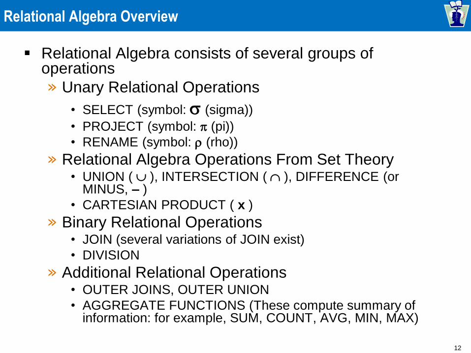
Relational Algebra consists of several groups of operations
» Unary Relational Operations
• SELECT (symbol: (sigma))
• PROJECT (symbol: (pi))
• RENAME (symbol: (rho))
» Relational Algebra Operations From Set Theory • UNION ( ), INTERSECTION ( ), DIFFERENCE (or
MINUS, – )
• CARTESIAN PRODUCT ( x )
» Binary Relational Operations • JOIN (several variations of JOIN exist)
• DIVISION
» Additional Relational Operations • OUTER JOINS, OUTER UNION
• AGGREGATE FUNCTIONS (These compute summary of information: for example, SUM, COUNT, AVG, MIN, MAX)
13
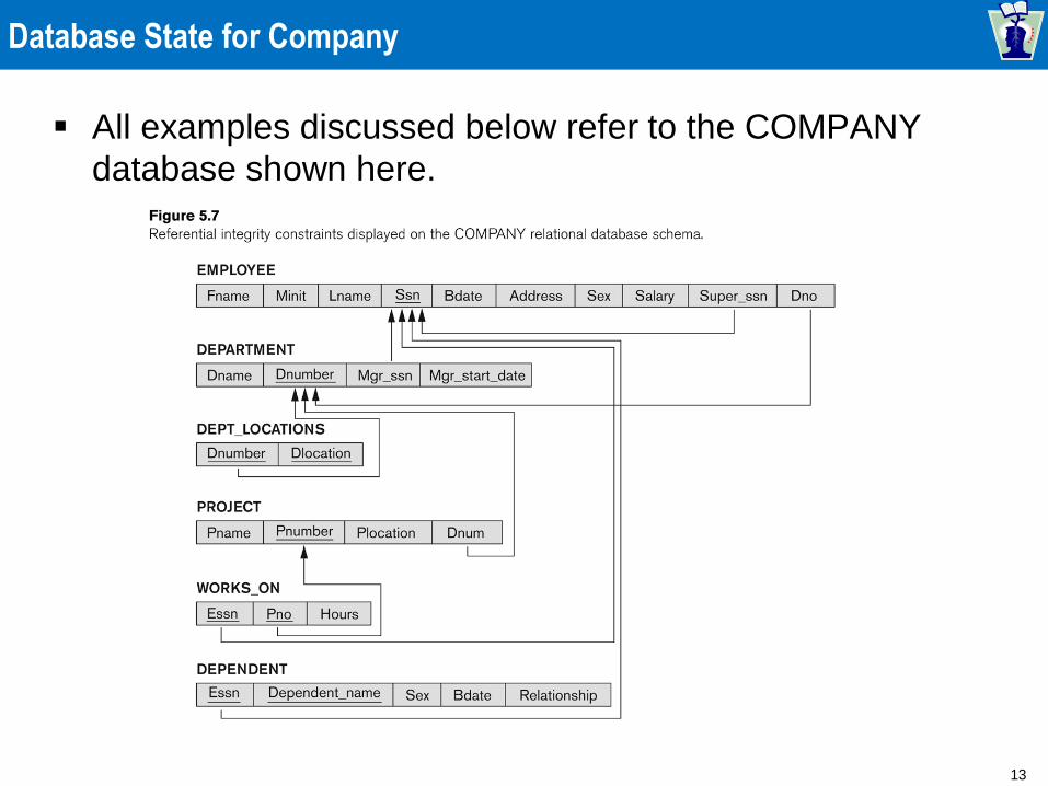
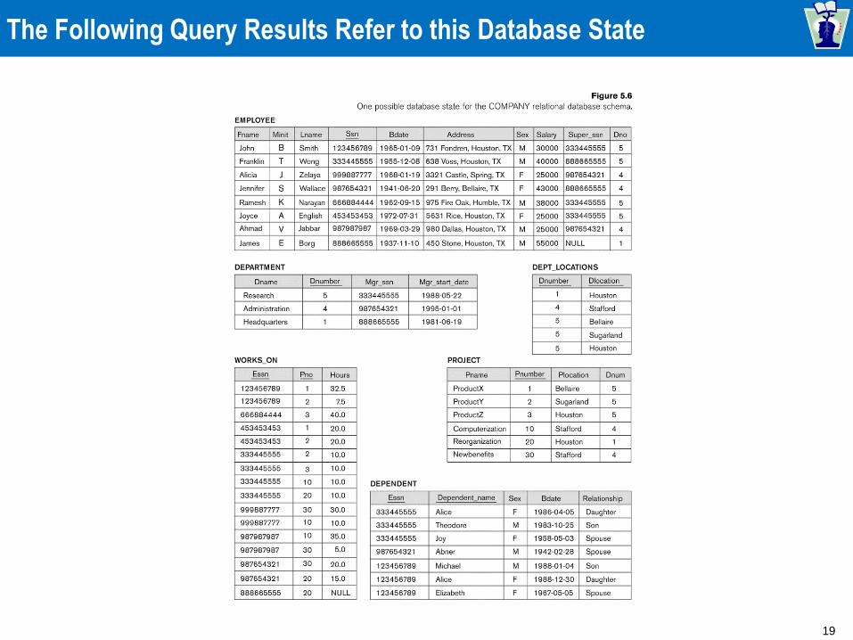
Database State for Company
All examples discussed below refer to the COMPANY
database shown here.
14
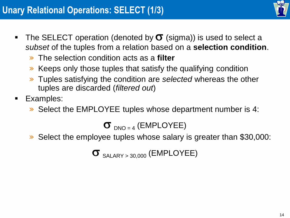
Unary Relational Operations: SELECT (1/3)
The SELECT operation (denoted by (sigma)) is used to select a
subset of the tuples from a relation based on a selection condition.
» The selection condition acts as a filter
» Keeps only those tuples that satisfy the qualifying condition
» Tuples satisfying the condition are selected whereas the other tuples are discarded (filtered out)
Examples:
» Select the EMPLOYEE tuples whose department number is 4:
DNO = 4 (EMPLOYEE)
» Select the employee tuples whose salary is greater than $30,000:
SALARY > 30,000 (EMPLOYEE)
15
Unary Relational Operations: SELECT (2/3)
» In general, the select operation is denoted by
<selection condition>(R) where
• the symbol (sigma) is used to denote the select
operator
• the selection condition is a Boolean (conditional)
expression specified on the attributes of relation R
• tuples that make the condition true are selected
– appear in the result of the operation
• tuples that make the condition false are filtered out
– discarded from the result of the operation
16
Unary Relational Operations: SELECT (3/3)
SELECT Operation Properties
» The SELECT operation <selection condition>(R) produces a relation S
that has the same schema (same attributes) as R
» SELECT is commutative:
<condition1>( < condition2> (R)) = <condition2> ( < condition1> (R))
» Because of commutativity property, a cascade (sequence) of SELECT operations may be applied in any order:
<cond1>(<cond2> (<cond3> (R)) = <cond2> (<cond3> (<cond1> ( R)))
» A cascade of SELECT operations may be replaced by a single selection with a conjunction of all the conditions:
<cond1>(< cond2> (<cond3>(R)) = <cond1> AND < cond2> AND <
cond3>(R)))
» The number of tuples in the result of a SELECT is less than (or equal to) the number of tuples in the input relation R
17
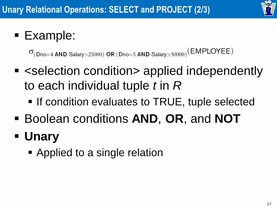
Unary Relational Operations: SELECT and PROJECT (2/3)
Example:
<selection condition> applied independently
to each individual tuple t in R
If condition evaluates to TRUE, tuple selected
Boolean conditions AND, OR, and NOT
Unary
Applied to a single relation
18
Unary Relational Operations: SELECT and PROJECT (3/3)
Selectivity
Fraction of tuples selected by a selection
condition
SELECT operation commutative
Cascade SELECT operations into a single
operation with AND condition
19
The Following Query Results Refer to this Database State
20
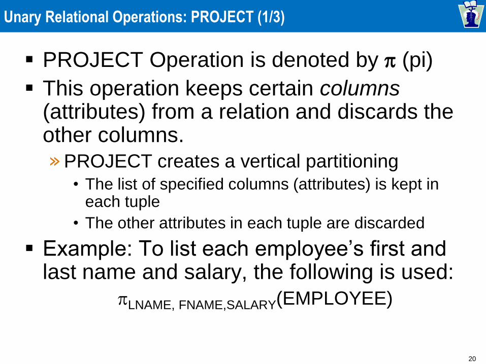
Unary Relational Operations: PROJECT (1/3)
PROJECT Operation is denoted by (pi)
This operation keeps certain columns (attributes) from a relation and discards the other columns.
» PROJECT creates a vertical partitioning • The list of specified columns (attributes) is kept in
each tuple
• The other attributes in each tuple are discarded
Example: To list each employee’s first and last name and salary, the following is used:
LNAME, FNAME,SALARY(EMPLOYEE)
21
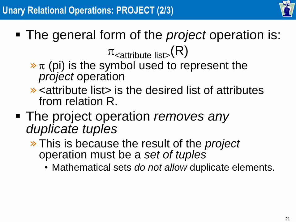
Unary Relational Operations: PROJECT (2/3)
The general form of the project operation is:
<attribute list>(R) » (pi) is the symbol used to represent the
project operation
» <attribute list> is the desired list of attributes from relation R.
The project operation removes any duplicate tuples » This is because the result of the project
operation must be a set of tuples • Mathematical sets do not allow duplicate elements.
22
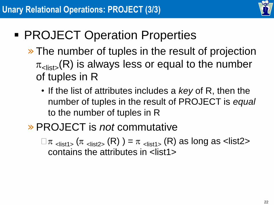
Unary Relational Operations: PROJECT (3/3)
PROJECT Operation Properties
» The number of tuples in the result of projection
<list>(R) is always less or equal to the number
of tuples in R
• If the list of attributes includes a key of R, then the
number of tuples in the result of PROJECT is equal
to the number of tuples in R
» PROJECT is not commutative
<list1> ( <list2> (R) ) = <list1> (R) as long as <list2>
contains the attributes in <list1>
23
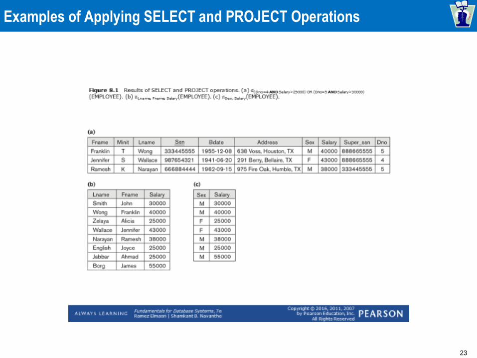
Examples of Applying SELECT and PROJECT Operations
24
Relational Algebra Expressions
We may want to apply several relational
algebra operations one after the other
» Either we can write the operations as a single
relational algebra expression by nesting the
operations, or
» We can apply one operation at a time and
create intermediate result relations.
In the latter case, we must give names to the
relations that hold the intermediate results.
25
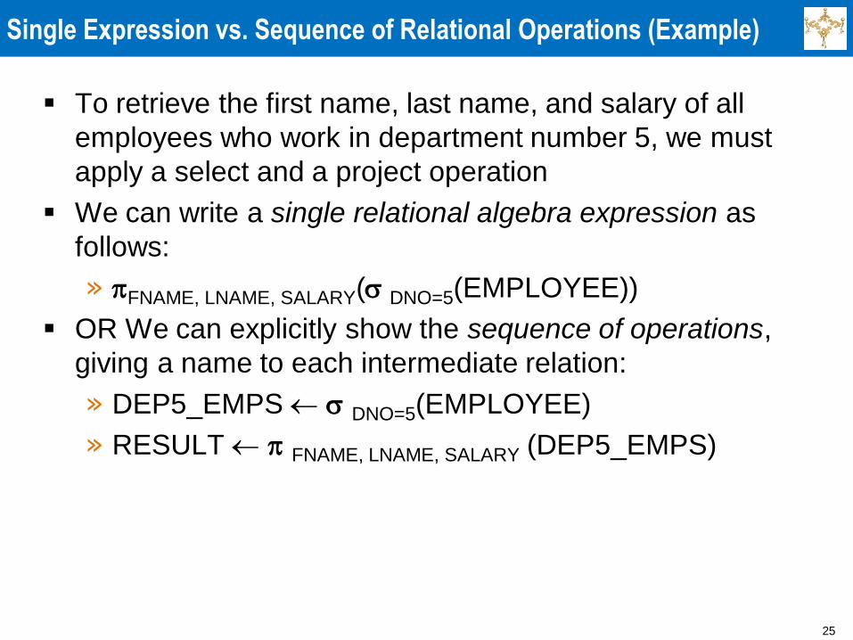
Single Expression vs. Sequence of Relational Operations (Example)
To retrieve the first name, last name, and salary of all
employees who work in department number 5, we must
apply a select and a project operation
We can write a single relational algebra expression as
follows:
» FNAME, LNAME, SALARY( DNO=5(EMPLOYEE))
OR We can explicitly show the sequence of operations,
giving a name to each intermediate relation:
» DEP5_EMPS DNO=5(EMPLOYEE)
» RESULT FNAME, LNAME, SALARY (DEP5_EMPS)
26
Unary Relational Operations: RENAME (1/3)
The RENAME operator is denoted by
(rho)
In some cases, we may want to rename the
attributes of a relation or the relation name
or both
» Useful when a query requires multiple
operations
» Necessary in some cases (see JOIN operation
later)
27
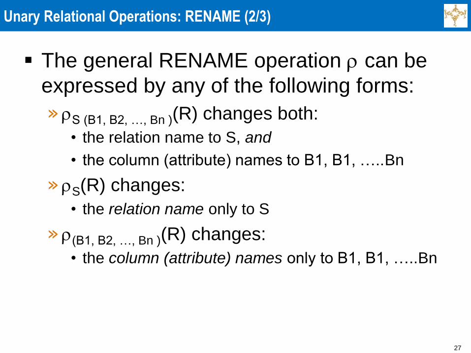
Unary Relational Operations: RENAME (2/3)
The general RENAME operation can be
expressed by any of the following forms:
» S (B1, B2, …, Bn )(R) changes both:
• the relation name to S, and
• the column (attribute) names to B1, B1, …..Bn
» S(R) changes:
• the relation name only to S
» (B1, B2, …, Bn )(R) changes:
• the column (attribute) names only to B1, B1, …..Bn
28
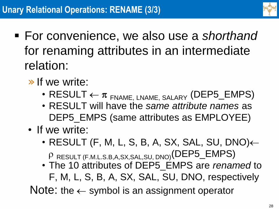
Unary Relational Operations: RENAME (3/3)
For convenience, we also use a shorthand
for renaming attributes in an intermediate
relation:
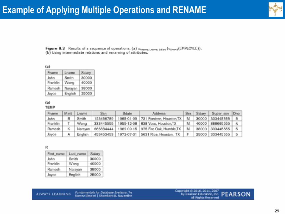
» If we write: • RESULT FNAME, LNAME, SALARY (DEP5_EMPS)
• RESULT will have the same attribute names as
DEP5_EMPS (same attributes as EMPLOYEE)
• If we write: • RESULT (F, M, L, S, B, A, SX, SAL, SU, DNO)
RESULT (F.M.L.S.B,A,SX,SAL,SU, DNO)(DEP5_EMPS)
• The 10 attributes of DEP5_EMPS are renamed to
F, M, L, S, B, A, SX, SAL, SU, DNO, respectively
Note: the symbol is an assignment operator
29
Example of Applying Multiple Operations and RENAME
30
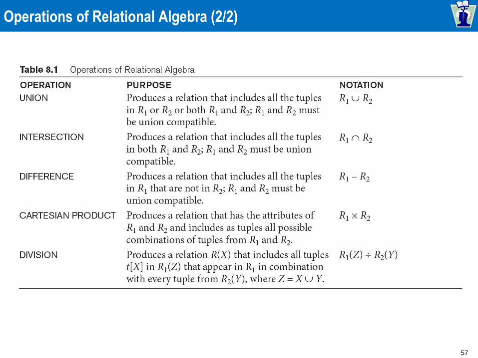
Relational Algebra Operations from Set Theory: UNION (1/2)
UNION Operation
» Binary operation, denoted by
» The result of R S, is a relation that includes all tuples that are either in R or in S or in both R and S
» Duplicate tuples are eliminated
» The two operand relations R and S must be “type compatible” (or UNION compatible)
• R and S must have same number of attributes
• Each pair of corresponding attributes must be type compatible (have same or compatible domains)
31
Relational Algebra Operations from Set Theory: UNION (2/2)
Example: » To retrieve the social security numbers of all employees who
either work in department 5 (RESULT1 below) or directly supervise an employee who works in department 5 (RESULT2 below)
» We can use the UNION operation as follows:
DEP5_EMPS DNO=5 (EMPLOYEE)
RESULT1 SSN(DEP5_EMPS)
RESULT2(SSN) SUPERSSN(DEP5_EMPS)
RESULT RESULT1 RESULT2 » The union operation produces the tuples that are in either
RESULT1 or RESULT2 or both
32
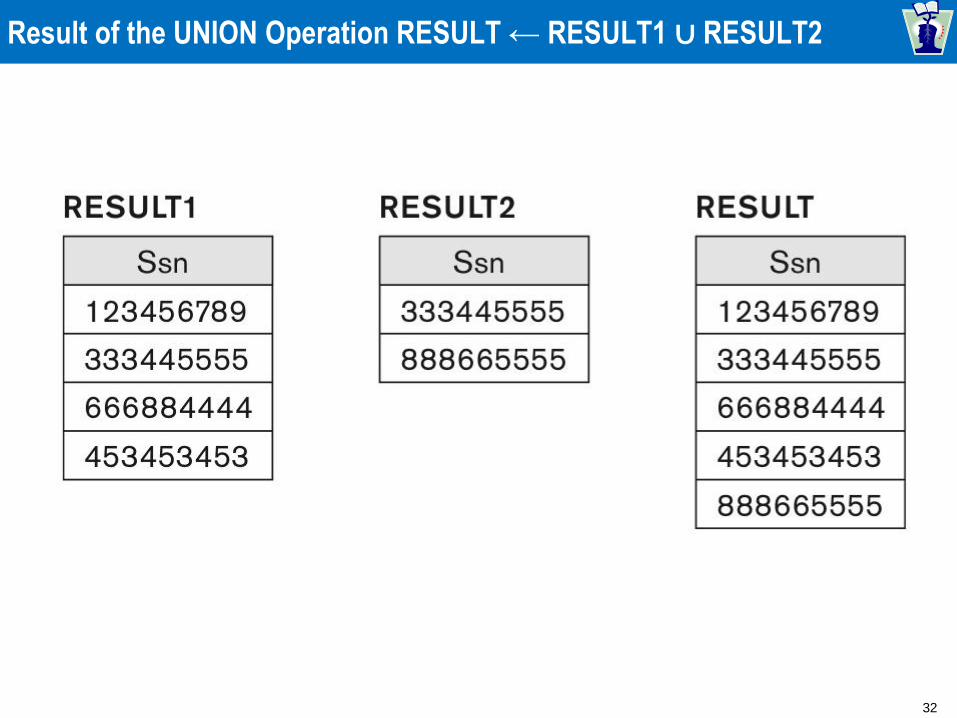
Result of the UNION Operation RESULT ← RESULT1 ∪ RESULT2
33
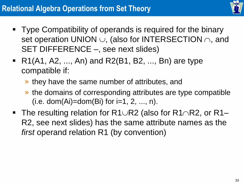
Relational Algebra Operations from Set Theory
Type Compatibility of operands is required for the binary
set operation UNION , (also for INTERSECTION , and
SET DIFFERENCE –, see next slides)
R1(A1, A2, ..., An) and R2(B1, B2, ..., Bn) are type
compatible if:
» they have the same number of attributes, and
» the domains of corresponding attributes are type compatible
(i.e. dom(Ai)=dom(Bi) for i=1, 2, ..., n).
The resulting relation for R1R2 (also for R1R2, or R1–
R2, see next slides) has the same attribute names as the
first operand relation R1 (by convention)
34
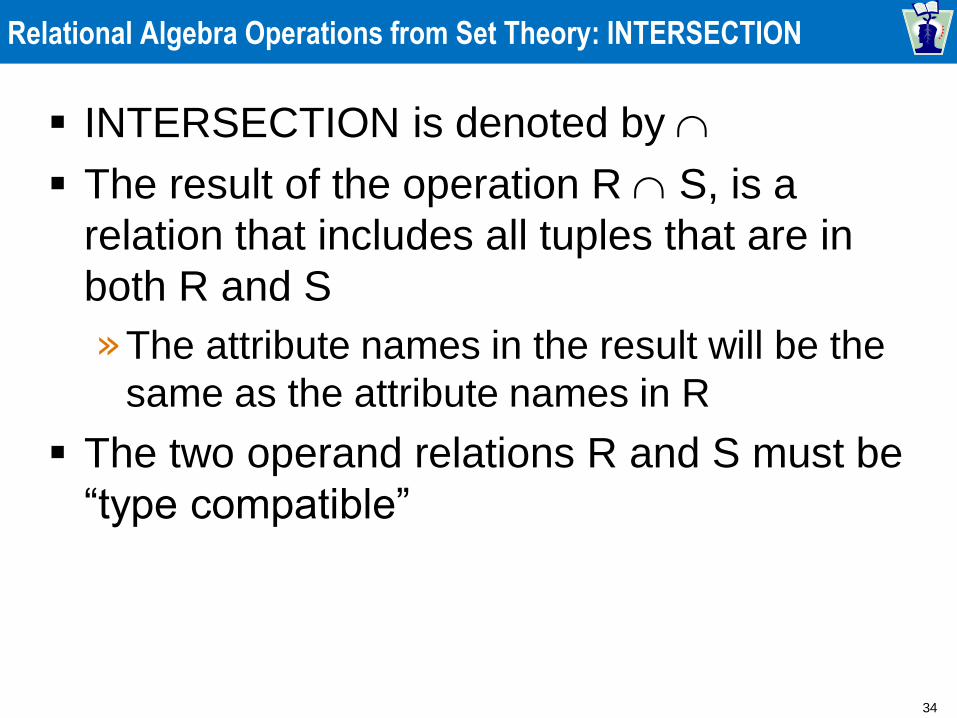
Relational Algebra Operations from Set Theory: INTERSECTION
INTERSECTION is denoted by
The result of the operation R S, is a
relation that includes all tuples that are in
both R and S
»The attribute names in the result will be the
same as the attribute names in R
The two operand relations R and S must be
“type compatible”
35
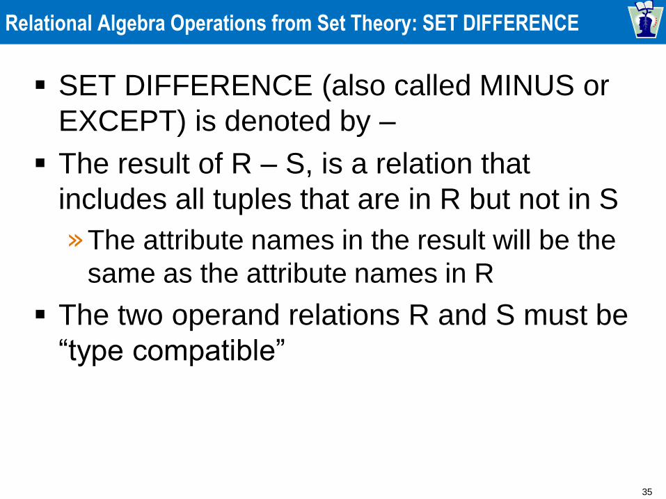
Relational Algebra Operations from Set Theory: SET DIFFERENCE
SET DIFFERENCE (also called MINUS or
EXCEPT) is denoted by –
The result of R – S, is a relation that
includes all tuples that are in R but not in S
»The attribute names in the result will be the
same as the attribute names in R
The two operand relations R and S must be
“type compatible”
36
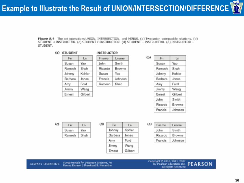
Example to Illustrate the Result of UNION/INTERSECTION/DIFFERENCE
37
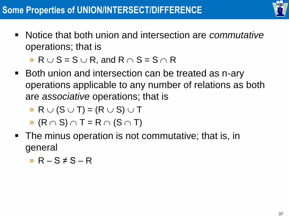
Some Properties of UNION/INTERSECT/DIFFERENCE
Notice that both union and intersection are commutative
operations; that is
» R S = S R, and R S = S R
Both union and intersection can be treated as n-ary
operations applicable to any number of relations as both
are associative operations; that is
» R (S T) = (R S) T
» (R S) T = R (S T)
The minus operation is not commutative; that is, in
general
» R – S ≠ S – R
38
Relational Algebra Operations from Set Theory: CARTESIAN PRODUCT
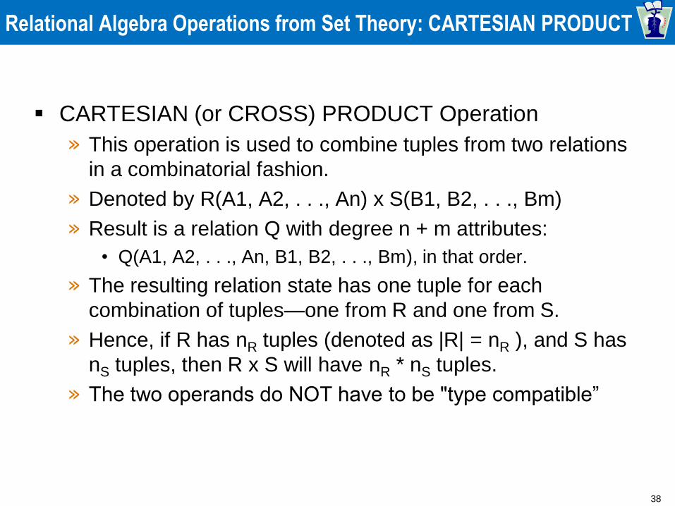
CARTESIAN (or CROSS) PRODUCT Operation
» This operation is used to combine tuples from two relations
in a combinatorial fashion.
» Denoted by R(A1, A2, . . ., An) x S(B1, B2, . . ., Bm)
» Result is a relation Q with degree n + m attributes:
• Q(A1, A2, . . ., An, B1, B2, . . ., Bm), in that order.
» The resulting relation state has one tuple for each
combination of tuples—one from R and one from S.
» Hence, if R has nR tuples (denoted as |R| = nR ), and S has
nS tuples, then R x S will have nR * nS tuples.
» The two operands do NOT have to be "type compatible”
39
Relational Algebra Operations from Set Theory: CARTESIAN PRODUCT
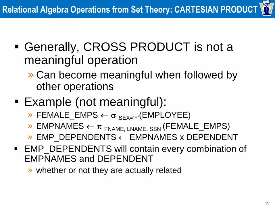
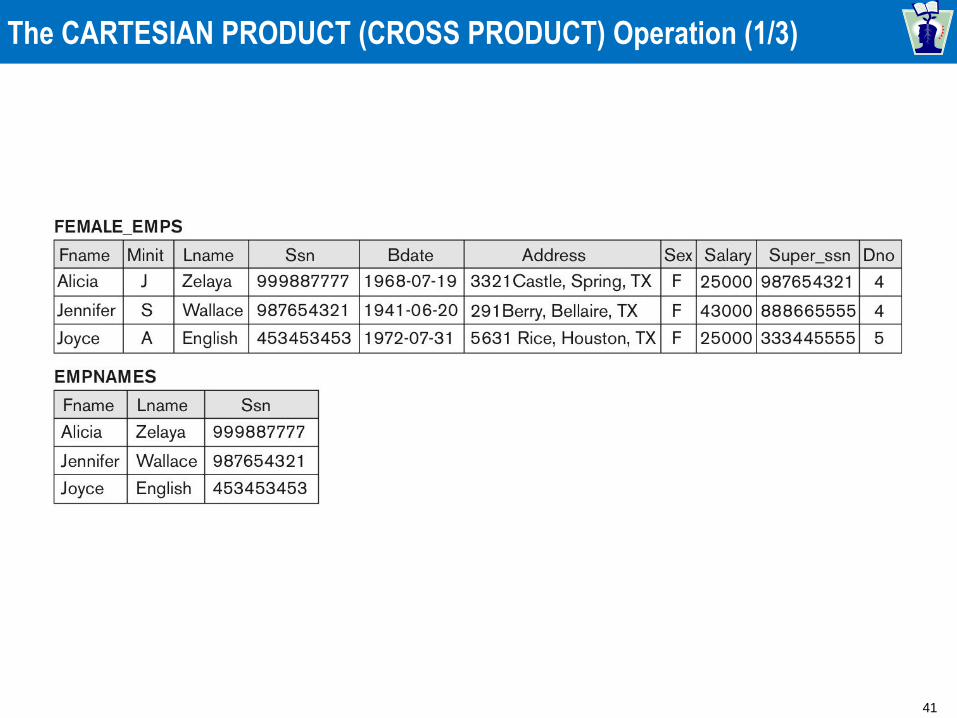
Generally, CROSS PRODUCT is not a meaningful operation
» Can become meaningful when followed by other operations
Example (not meaningful): » FEMALE_EMPS SEX=’F’(EMPLOYEE)
» EMPNAMES FNAME, LNAME, SSN (FEMALE_EMPS)
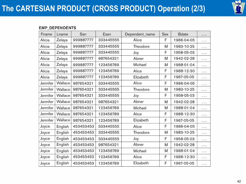
» EMP_DEPENDENTS EMPNAMES x DEPENDENT
EMP_DEPENDENTS will contain every combination of EMPNAMES and DEPENDENT
» whether or not they are actually related
40
Relational Algebra Operations from Set Theory: CARTESIAN PRODUCT
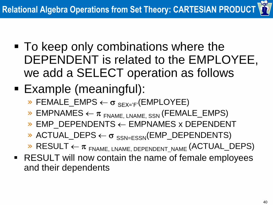
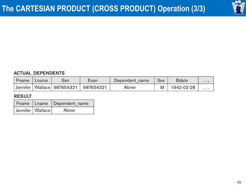
To keep only combinations where the DEPENDENT is related to the EMPLOYEE, we add a SELECT operation as follows
Example (meaningful): » FEMALE_EMPS SEX=’F’(EMPLOYEE)
» EMPNAMES FNAME, LNAME, SSN (FEMALE_EMPS)
» EMP_DEPENDENTS EMPNAMES x DEPENDENT
» ACTUAL_DEPS SSN=ESSN(EMP_DEPENDENTS)
» RESULT FNAME, LNAME, DEPENDENT_NAME (ACTUAL_DEPS)
RESULT will now contain the name of female employees and their dependents
41
The CARTESIAN PRODUCT (CROSS PRODUCT) Operation (1/3)
42
The CARTESIAN PRODUCT (CROSS PRODUCT) Operation (2/3)
43
The CARTESIAN PRODUCT (CROSS PRODUCT) Operation (3/3)
44
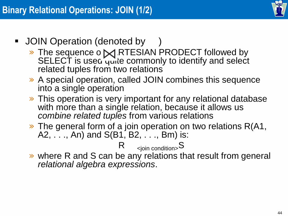
Binary Relational Operations: JOIN (1/2)
JOIN Operation (denoted by ) » The sequence of CARTESIAN PRODECT followed by
SELECT is used quite commonly to identify and select related tuples from two relations
» A special operation, called JOIN combines this sequence into a single operation
» This operation is very important for any relational database with more than a single relation, because it allows us combine related tuples from various relations
» The general form of a join operation on two relations R(A1, A2, . . ., An) and S(B1, B2, . . ., Bm) is:
R <join condition>S
» where R and S can be any relations that result from general relational algebra expressions.
45
Binary Relational Operations: JOIN (2/2)
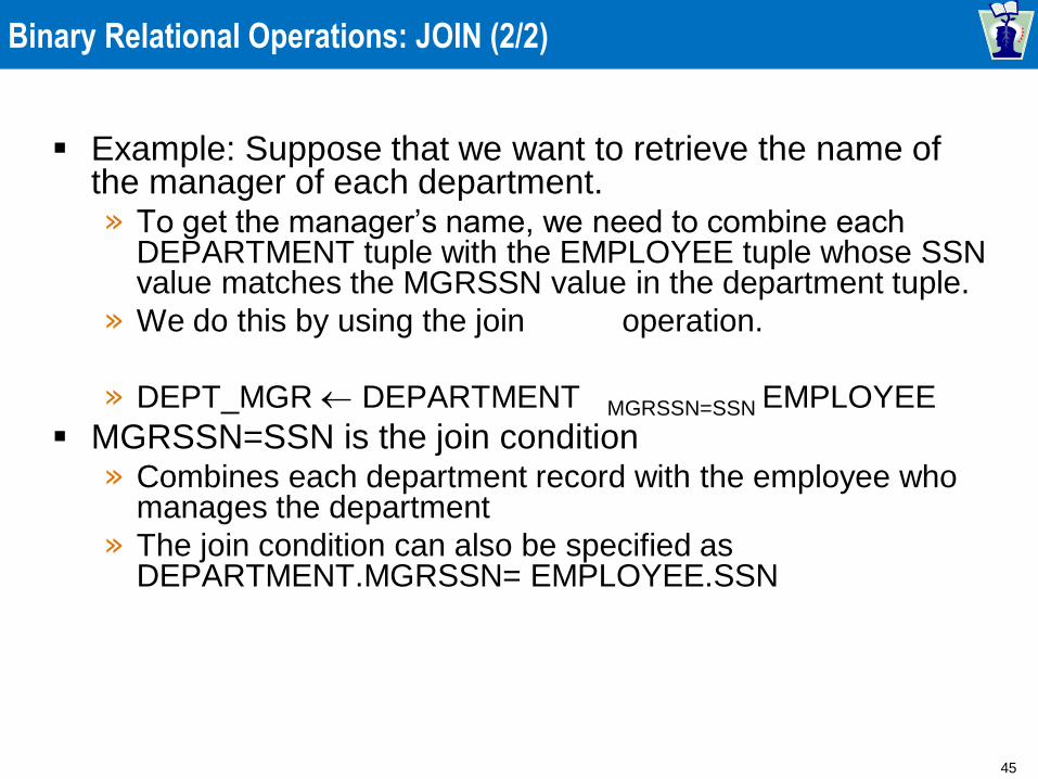
Example: Suppose that we want to retrieve the name of the manager of each department. » To get the manager’s name, we need to combine each
DEPARTMENT tuple with the EMPLOYEE tuple whose SSN value matches the MGRSSN value in the department tuple.
» We do this by using the join operation.
» DEPT_MGR DEPARTMENT MGRSSN=SSN EMPLOYEE
MGRSSN=SSN is the join condition » Combines each department record with the employee who
manages the department
» The join condition can also be specified as DEPARTMENT.MGRSSN= EMPLOYEE.SSN
46
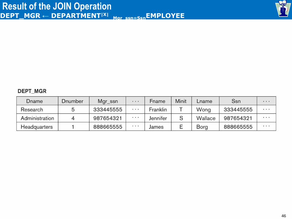
Result of the JOIN Operation DEPT_MGR ← DEPARTMENT|X| Mgr_ssn=SsnEMPLOYEE
47
Some Properties of JOIN (1/2)
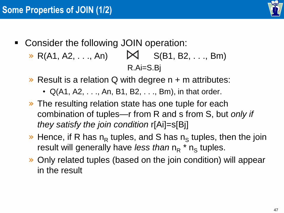
Consider the following JOIN operation:
» R(A1, A2, . . ., An) S(B1, B2, . . ., Bm)
R.Ai=S.Bj
» Result is a relation Q with degree n + m attributes:
• Q(A1, A2, . . ., An, B1, B2, . . ., Bm), in that order.
» The resulting relation state has one tuple for each
combination of tuples—r from R and s from S, but only if
they satisfy the join condition r[Ai]=s[Bj]
» Hence, if R has nR tuples, and S has nS tuples, then the join
result will generally have less than nR * nS tuples.
» Only related tuples (based on the join condition) will appear
in the result
48
Binary Relational Operations: JOIN (2/2)
The general case of JOIN operation is called a Theta-join: R S
theta
The join condition is called theta
Theta can be any general boolean expression on the attributes of R and S; for example:
» R.Ai<S.Bj AND (R.Ak=S.Bl OR R.Ap<S.Bq)
Most join conditions involve one or more equality conditions “AND”ed together; for example:
» R.Ai=S.Bj AND R.Ak=S.Bl AND R.Ap=S.Bq
49
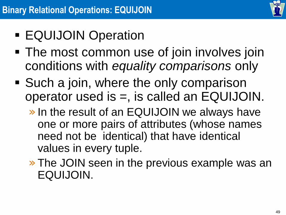
Binary Relational Operations: EQUIJOIN
EQUIJOIN Operation
The most common use of join involves join conditions with equality comparisons only
Such a join, where the only comparison operator used is =, is called an EQUIJOIN.
» In the result of an EQUIJOIN we always have one or more pairs of attributes (whose names need not be identical) that have identical values in every tuple.
» The JOIN seen in the previous example was an EQUIJOIN.
50
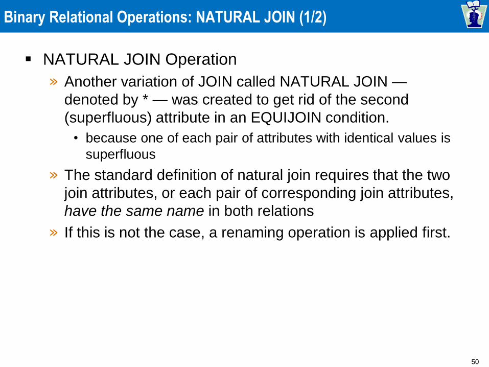
Binary Relational Operations: NATURAL JOIN (1/2)
NATURAL JOIN Operation
» Another variation of JOIN called NATURAL JOIN —
denoted by * — was created to get rid of the second
(superfluous) attribute in an EQUIJOIN condition.
• because one of each pair of attributes with identical values is
superfluous
» The standard definition of natural join requires that the two
join attributes, or each pair of corresponding join attributes,
have the same name in both relations
» If this is not the case, a renaming operation is applied first.
51
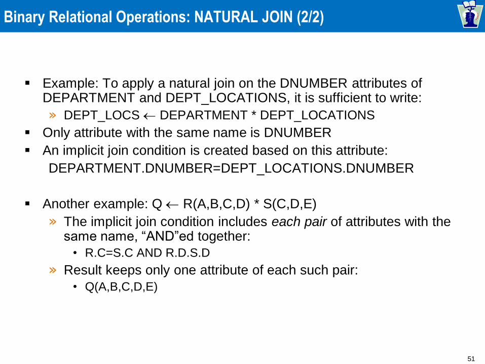
Binary Relational Operations: NATURAL JOIN (2/2)
Example: To apply a natural join on the DNUMBER attributes of DEPARTMENT and DEPT_LOCATIONS, it is sufficient to write:
» DEPT_LOCS DEPARTMENT * DEPT_LOCATIONS
Only attribute with the same name is DNUMBER
An implicit join condition is created based on this attribute:
DEPARTMENT.DNUMBER=DEPT_LOCATIONS.DNUMBER
Another example: Q R(A,B,C,D) * S(C,D,E)
» The implicit join condition includes each pair of attributes with the same name, “AND”ed together:
• R.C=S.C AND R.D.S.D
» Result keeps only one attribute of each such pair:
• Q(A,B,C,D,E)
52
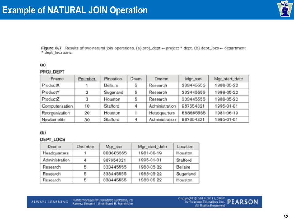
Example of NATURAL JOIN Operation
53
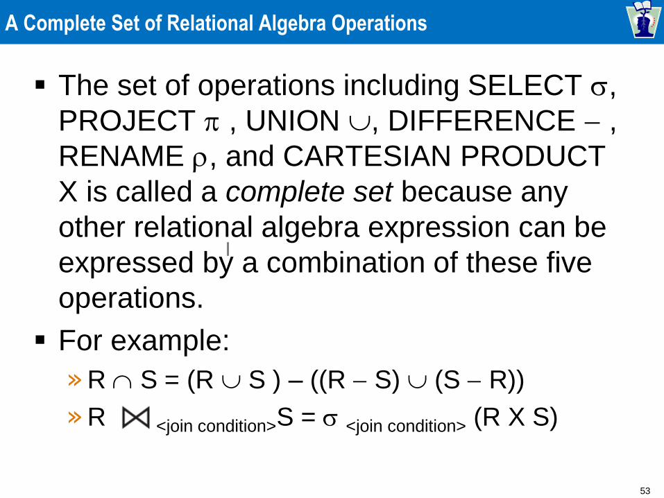
A Complete Set of Relational Algebra Operations
The set of operations including SELECT ,
PROJECT , UNION , DIFFERENCE - ,
RENAME , and CARTESIAN PRODUCT
X is called a complete set because any
other relational algebra expression can be
expressed by a combination of these five
operations.
For example:
» R S = (R S ) – ((R - S) (S - R))
» R <join condition>S = <join condition> (R X S)
54
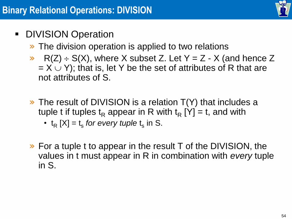
Binary Relational Operations: DIVISION
DIVISION Operation
» The division operation is applied to two relations
» R(Z) S(X), where X subset Z. Let Y = Z - X (and hence Z = X Y); that is, let Y be the set of attributes of R that are not attributes of S.
» The result of DIVISION is a relation T(Y) that includes a tuple t if tuples tR appear in R with tR [Y] = t, and with
• tR [X] = ts for every tuple ts in S.
» For a tuple t to appear in the result T of the DIVISION, the values in t must appear in R in combination with every tuple in S.
55
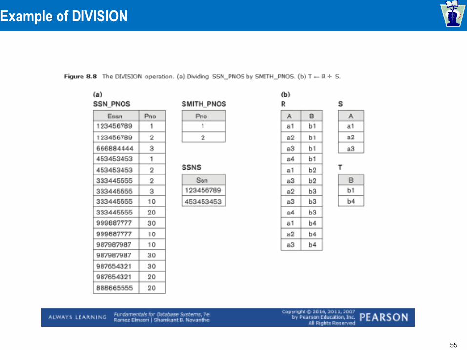
Example of DIVISION
56
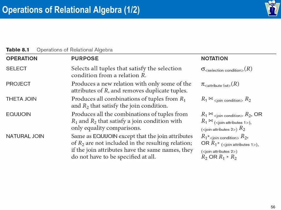
Operations of Relational Algebra (1/2)
57
Operations of Relational Algebra (2/2)
58
Query Tree Notation
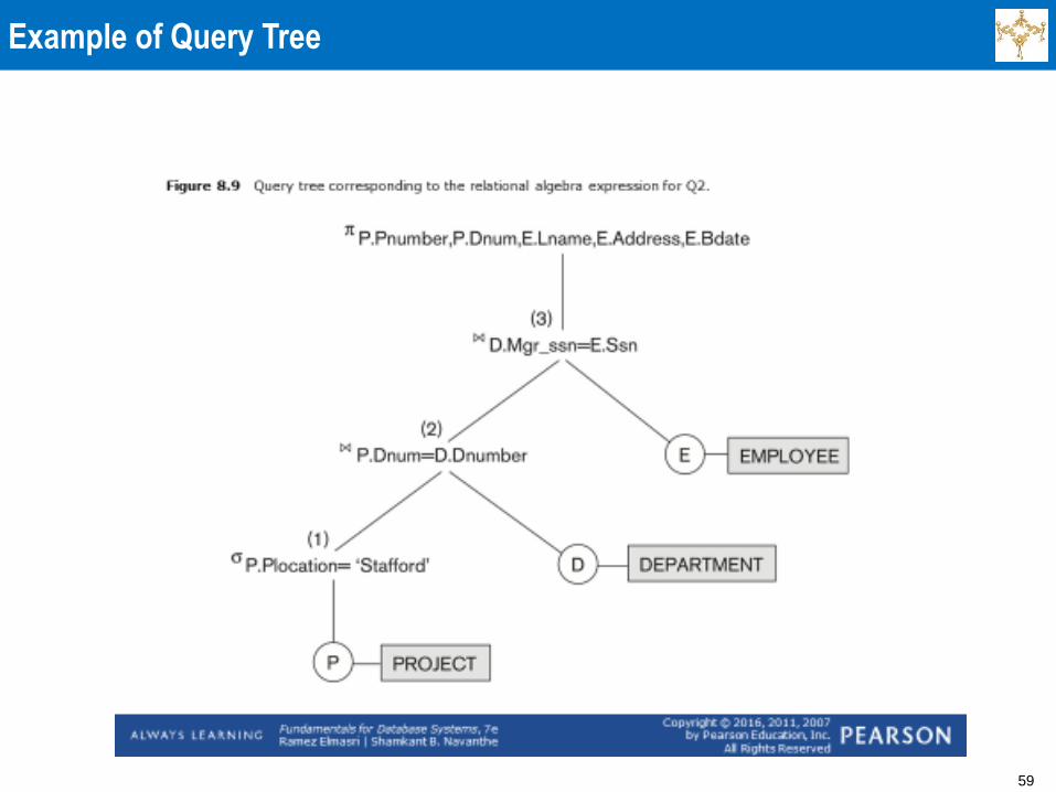
Query Tree
» An internal data structure to represent a query
» Standard technique for estimating the work involved in executing the query, the generation of intermediate results, and the optimization of execution
» Nodes stand for operations like selection, projection, join, renaming, division, ….
» Leaf nodes represent base relations
» A tree gives a good visual feel of the complexity of the query and the operations involved
» Algebraic Query Optimization consists of rewriting the query or modifying the query tree into an equivalent tree
» (See Textbook Chapter 15)
59
Example of Query Tree
60
Additional Relational Operations: Aggregate Functions & Grouping
A type of request that cannot be expressed in the basic relational algebra is to specify mathematical aggregate functions on collections of values from the database.
Examples of such functions include retrieving the average or total salary of all employees or the total number of employee tuples. » These functions are used in simple statistical queries that
summarize information from the database tuples.
Common functions applied to collections of numeric values include » SUM, AVERAGE, MAXIMUM, and MINIMUM.
The COUNT function is used for counting tuples or values.
61
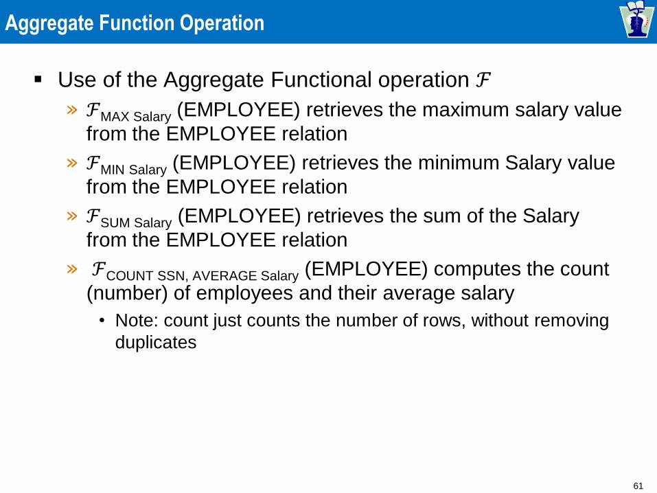
Aggregate Function Operation
Use of the Aggregate Functional operation ℱ
» ℱMAX Salary (EMPLOYEE) retrieves the maximum salary value
from the EMPLOYEE relation
» ℱMIN Salary (EMPLOYEE) retrieves the minimum Salary value
from the EMPLOYEE relation
» ℱSUM Salary (EMPLOYEE) retrieves the sum of the Salary
from the EMPLOYEE relation
» ℱCOUNT SSN, AVERAGE Salary (EMPLOYEE) computes the count
(number) of employees and their average salary
• Note: count just counts the number of rows, without removing
duplicates
62
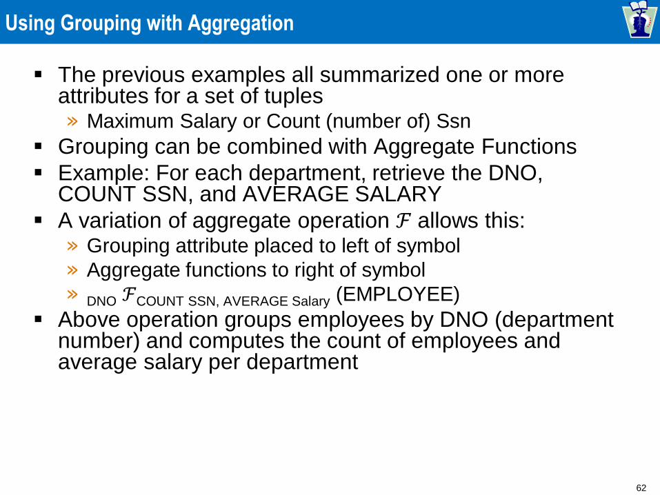
Using Grouping with Aggregation
The previous examples all summarized one or more attributes for a set of tuples » Maximum Salary or Count (number of) Ssn
Grouping can be combined with Aggregate Functions
Example: For each department, retrieve the DNO, COUNT SSN, and AVERAGE SALARY
A variation of aggregate operation ℱ allows this: » Grouping attribute placed to left of symbol
» Aggregate functions to right of symbol
» DNO ℱCOUNT SSN, AVERAGE Salary (EMPLOYEE)
Above operation groups employees by DNO (department number) and computes the count of employees and average salary per department
63
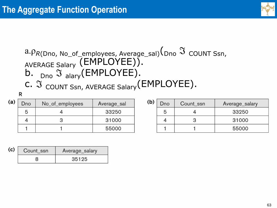
The Aggregate Function Operation
a.ρR(Dno, No_of_employees, Average_sal)(Dno ℑ COUNT Ssn,
AVERAGE Salary (EMPLOYEE)). b. Dno ℑ alary(EMPLOYEE). c. ℑ COUNT Ssn, AVERAGE Salary(EMPLOYEE).
64
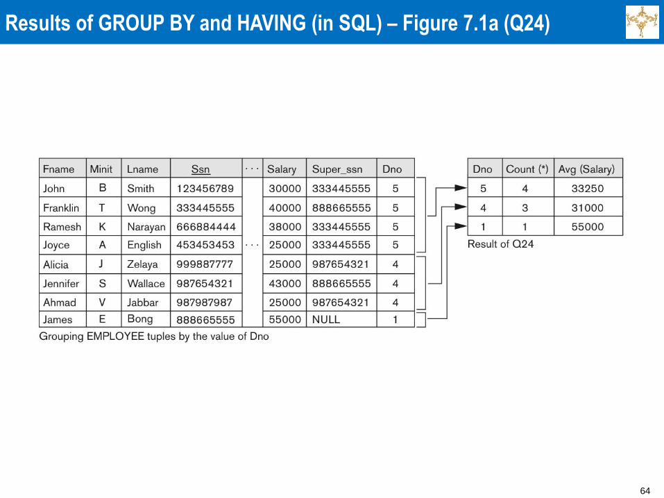
Results of GROUP BY and HAVING (in SQL) – Figure 7.1a (Q24)
65
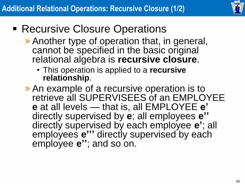
Additional Relational Operations: Recursive Closure (1/2)
Recursive Closure Operations » Another type of operation that, in general,
cannot be specified in the basic original relational algebra is recursive closure.
• This operation is applied to a recursive relationship.
» An example of a recursive operation is to retrieve all SUPERVISEES of an EMPLOYEE e at all levels — that is, all EMPLOYEE e’ directly supervised by e; all employees e’’ directly supervised by each employee e’; all employees e’’’ directly supervised by each employee e’’; and so on.
66
Additional Relational Operations: Recursive Closure (2/2)
Although it is possible to retrieve
employees at each level and then take their
union, we cannot, in general, specify a
query such as “retrieve the supervisees of
‘James Borg’ at all levels” without utilizing a
looping mechanism.
» The SQL3 standard includes syntax for
recursive closure.
67
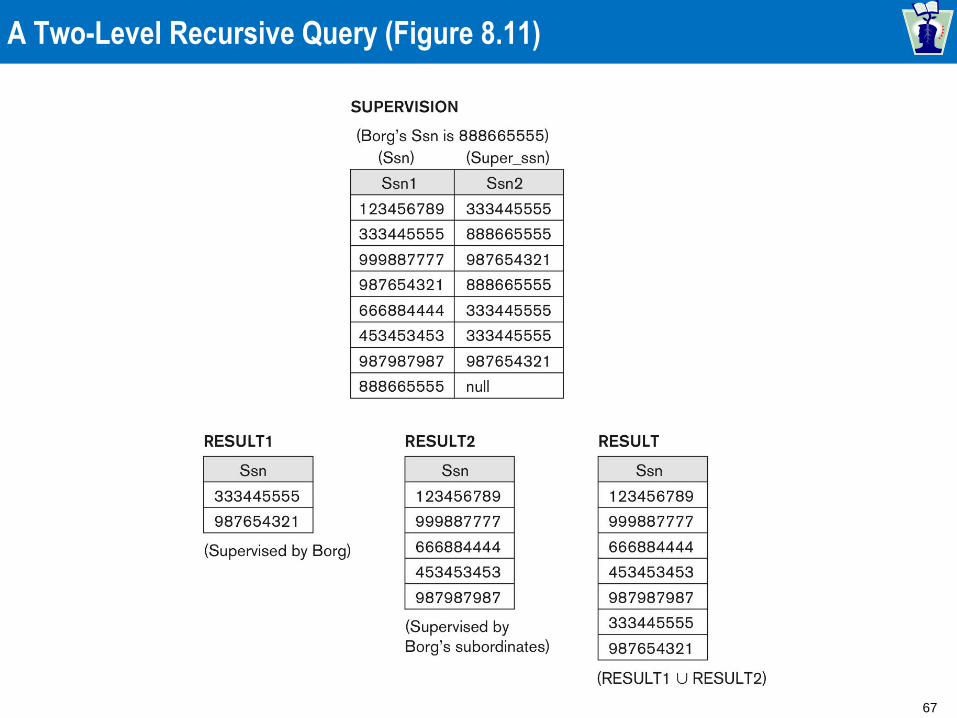
A Two-Level Recursive Query (Figure 8.11)
68
Additional Relational Operations: OUTER JOIN (1/2)
The OUTER JOIN Operation
» In NATURAL JOIN and EQUIJOIN, tuples without a
matching (or related) tuple are eliminated from the join result
• Tuples with null in the join attributes are also eliminated
• This amounts to loss of information.
» A set of operations, called OUTER joins, can be used when
we want to keep all the tuples in R, or all those in S, or all
those in both relations in the result of the join, regardless of
whether or not they have matching tuples in the other
relation.
69
Additional Relational Operations: OUTER JOIN (2/2)
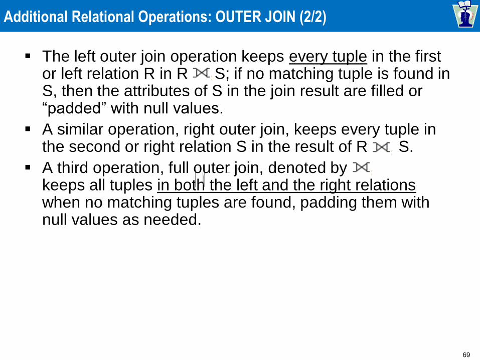
The left outer join operation keeps every tuple in the first or left relation R in R S; if no matching tuple is found in S, then the attributes of S in the join result are filled or “padded” with null values.
A similar operation, right outer join, keeps every tuple in the second or right relation S in the result of R S.
A third operation, full outer join, denoted by keeps all tuples in both the left and the right relations when no matching tuples are found, padding them with null values as needed.
70
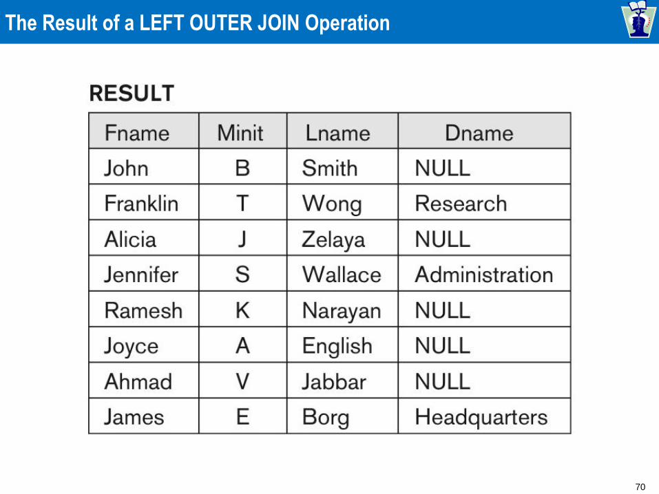
The Result of a LEFT OUTER JOIN Operation
71
Additional Relational Operations: OUTER UNION (1/2)
OUTER UNION Operations » The outer union operation was developed to
take the union of tuples from two relations if the relations are not type compatible.
» This operation will take the union of tuples in two relations R(X, Y) and S(X, Z) that are partially compatible, meaning that only some of their attributes, say X, are type compatible.
» The attributes that are type compatible are represented only once in the result, and those attributes that are not type compatible from either relation are also kept in the result relation T(X, Y, Z).
72
Additional Relational Operations: OUTER UNION (2/2)
Example: An outer union can be applied to two relations whose schemas are STUDENT(Name, SSN, Department, Advisor) and INSTRUCTOR(Name, SSN, Department, Rank). » Tuples from the two relations are matched based on having the
same combination of values of the shared attributes— Name, SSN, Department.
» If a student is also an instructor, both Advisor and Rank will have a value; otherwise, one of these two attributes will be null.
» The result relation STUDENT_OR_INSTRUCTOR will have the following attributes:
STUDENT_OR_INSTRUCTOR (Name, SSN, Department, Advisor, Rank)
73
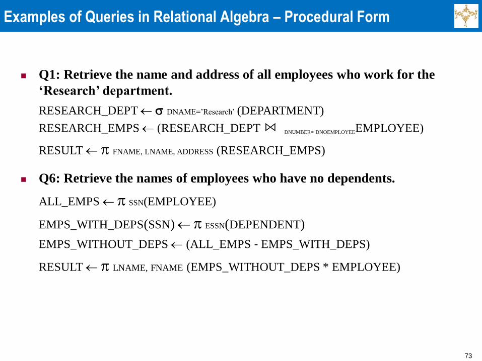
Examples of Queries in Relational Algebra – Procedural Form
Q1: Retrieve the name and address of all employees who work for the
‘Research’ department.
RESEARCH_DEPT DNAME=’Research’ (DEPARTMENT)
RESEARCH_EMPS (RESEARCH_DEPT DNUMBER= DNOEMPLOYEEEMPLOYEE)
RESULT FNAME, LNAME, ADDRESS (RESEARCH_EMPS)
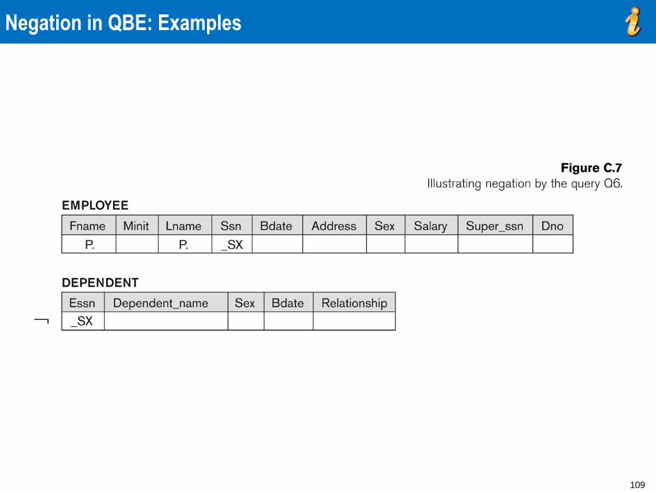
Q6: Retrieve the names of employees who have no dependents.
ALL_EMPS SSN(EMPLOYEE)
EMPS_WITH_DEPS(SSN) ESSN(DEPENDENT)
EMPS_WITHOUT_DEPS (ALL_EMPS - EMPS_WITH_DEPS)
RESULT LNAME, FNAME (EMPS_WITHOUT_DEPS * EMPLOYEE)
74
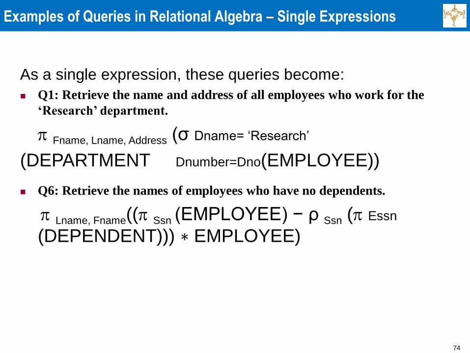
Examples of Queries in Relational Algebra – Single Expressions
As a single expression, these queries become:
Q1: Retrieve the name and address of all employees who work for the
‘Research’ department.
Fname, Lname, Address (σ Dname= ‘Research’
(DEPARTMENT Dnumber=Dno(EMPLOYEE))
Q6: Retrieve the names of employees who have no dependents.
Lname, Fname(( Ssn (EMPLOYEE) − ρ Ssn ( Essn
(DEPENDENT))) ∗ EMPLOYEE)
75
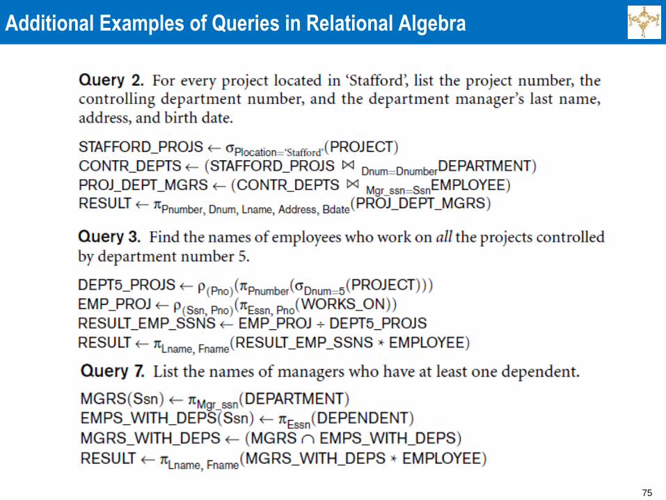
Additional Examples of Queries in Relational Algebra
76
Relational Calculus (1/2)
A relational calculus expression creates a new relation, which is specified in terms of variables that range over rows of the stored database relations (in tuple calculus) or over columns of the stored relations (in domain calculus).
In a calculus expression, there is no order of operations to specify how to retrieve the query result—a calculus expression specifies only what information the result should contain.
» This is the main distinguishing feature between relational algebra and relational calculus.
77
Relational Calculus (2/2)
Relational calculus is considered to be a
nonprocedural or declarative language.
This differs from relational algebra, where
we must write a sequence of operations to
specify a retrieval request; hence relational
algebra can be considered as a procedural
way of stating a query.
78
Tuple Relational Calculus (1/2)
The tuple relational calculus is based on specifying a
number of tuple variables.
Each tuple variable usually ranges over a particular
database relation, meaning that the variable may take as
its value any individual tuple from that relation.
A simple tuple relational calculus query is of the form
{t | COND(t)}
» where t is a tuple variable and COND (t) is a conditional
expression involving t.
» The result of such a query is the set of all tuples t that
satisfy COND (t).
79
Tuple Relational Calculus (2/2)
Example: To find the first and last names of all employees whose salary is above $50,000, we can write the following tuple calculus expression:
{t.FNAME, t.LNAME | EMPLOYEE(t) AND t.SALARY>50000}
The condition EMPLOYEE(t) specifies that the range relation of tuple variable t is EMPLOYEE.
The first and last name (PROJECTION FNAME, LNAME) of each EMPLOYEE tuple t that satisfies the condition t.SALARY>50000 (SELECTION SALARY >50000) will be retrieved.
80
Tuple Variables and Range Relations
Tuple variables
Ranges over a particular database relation
Satisfy COND(t):
Specify:
Range relation R of t
Select particular combinations of tuples
Set of attributes to be retrieved (requested
attributes)
81
Expressions and Formulas in Tuple Relational Calculus
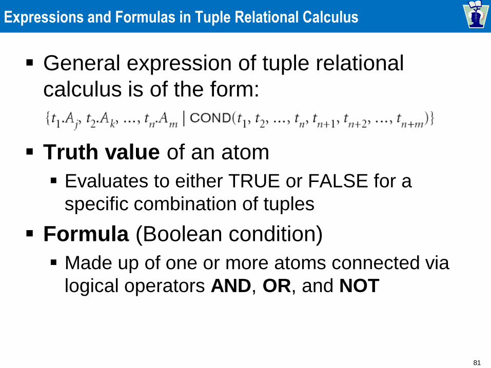
General expression of tuple relational
calculus is of the form:
Truth value of an atom
Evaluates to either TRUE or FALSE for a
specific combination of tuples
Formula (Boolean condition)
Made up of one or more atoms connected via
logical operators AND, OR, and NOT
82
The Existential and Universal Quantifiers (1/2)
Two special symbols called quantifiers can appear in formulas; these are the universal quantifier () and the existential quantifier ().
Informally, a tuple variable t is bound if it is quantified, meaning that it appears in an ( t) or ( t) clause; otherwise, it is free.
If F is a formula, then so are ( t)(F) and ( t)(F), where t is a tuple variable. » The formula ( t)(F) is true if the formula F evaluates to true
for some (at least one) tuple assigned to free occurrences of t in F; otherwise ( t)(F) is false.
» The formula ( t)(F) is true if the formula F evaluates to true for every tuple (in the universe) assigned to free occurrences of t in F; otherwise ( t)(F) is false.
83
The Existential and Universal Quantifiers (2/2)
is called the universal or “for all” quantifier because
every tuple in “the universe of” tuples must make F true to
make the quantified formula true.
is called the existential or “there exists” quantifier
because any tuple that exists in “the universe of” tuples
may make F true to make the quantified formula true.
84
Example Query Using Existential Quantifier
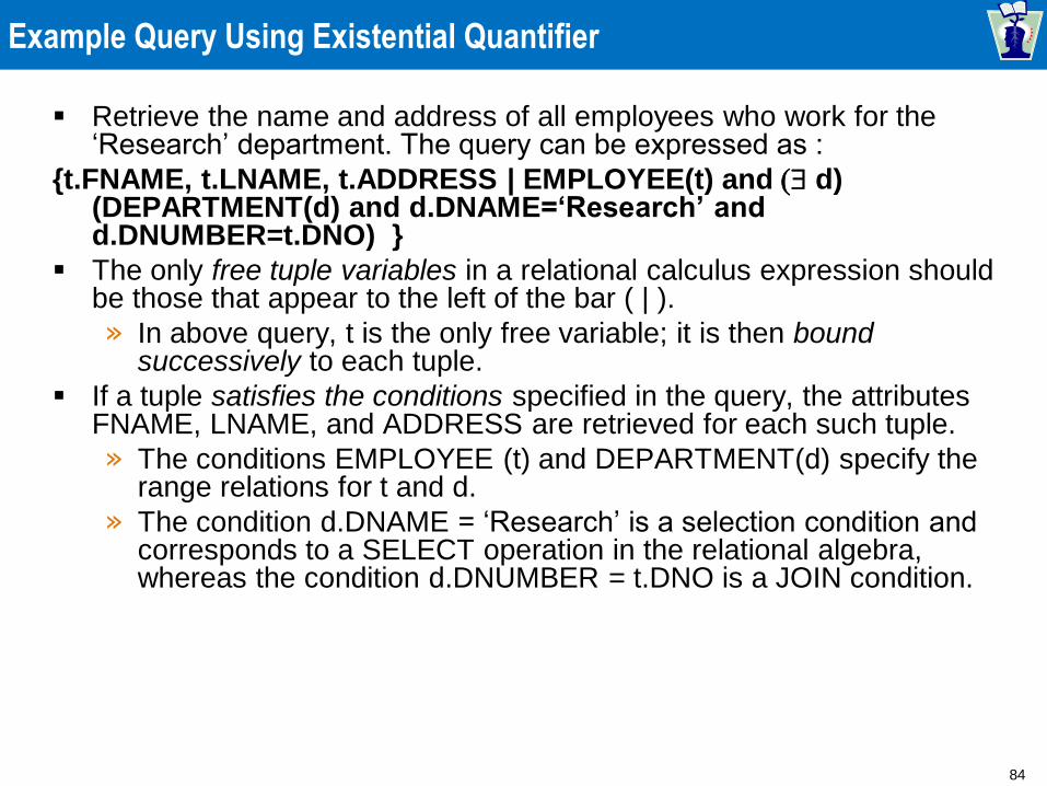
Retrieve the name and address of all employees who work for the ‘Research’ department. The query can be expressed as :
{t.FNAME, t.LNAME, t.ADDRESS | EMPLOYEE(t) and ( d) (DEPARTMENT(d) and d.DNAME=‘Research’ and d.DNUMBER=t.DNO) }
The only free tuple variables in a relational calculus expression should be those that appear to the left of the bar ( | ).
» In above query, t is the only free variable; it is then bound successively to each tuple.
If a tuple satisfies the conditions specified in the query, the attributes FNAME, LNAME, and ADDRESS are retrieved for each such tuple.
» The conditions EMPLOYEE (t) and DEPARTMENT(d) specify the range relations for t and d.
» The condition d.DNAME = ‘Research’ is a selection condition and corresponds to a SELECT operation in the relational algebra, whereas the condition d.DNUMBER = t.DNO is a JOIN condition.
85
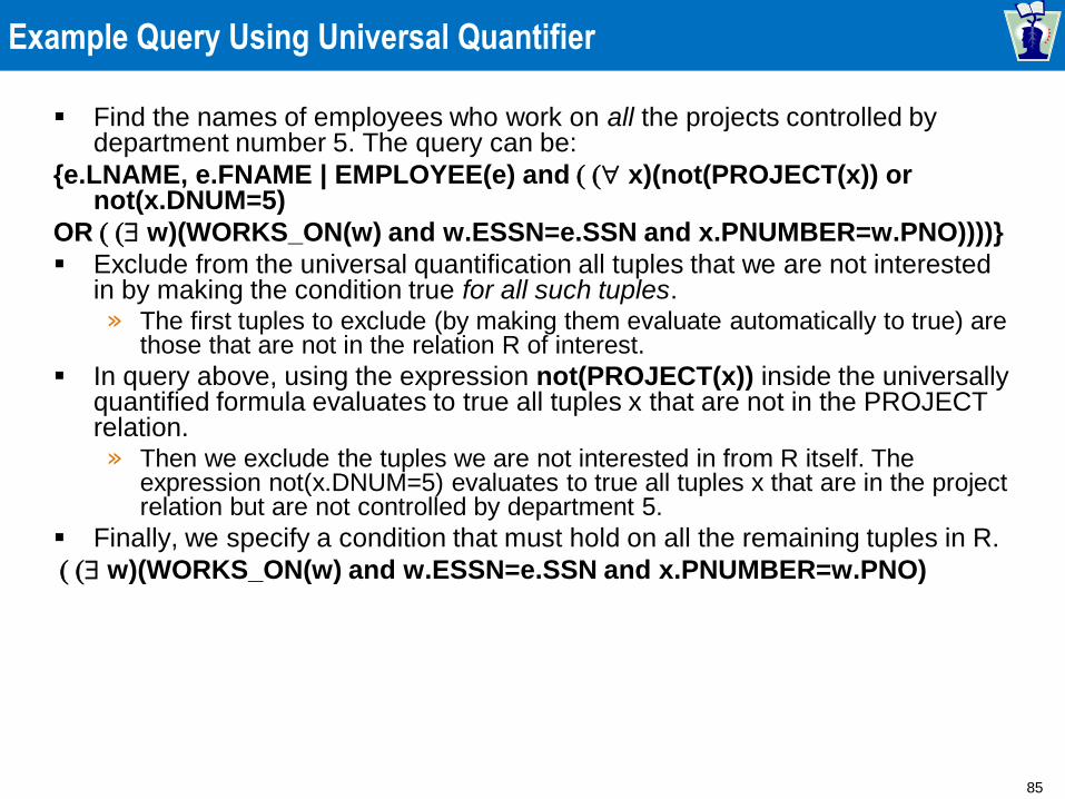
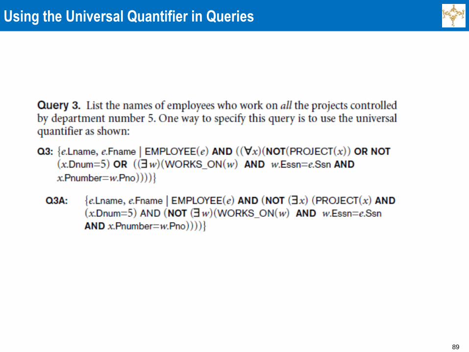
Example Query Using Universal Quantifier
Find the names of employees who work on all the projects controlled by department number 5. The query can be:
{e.LNAME, e.FNAME | EMPLOYEE(e) and ( ( x)(not(PROJECT(x)) or not(x.DNUM=5)
OR ( ( w)(WORKS_ON(w) and w.ESSN=e.SSN and x.PNUMBER=w.PNO))))}
Exclude from the universal quantification all tuples that we are not interested in by making the condition true for all such tuples. » The first tuples to exclude (by making them evaluate automatically to true) are
those that are not in the relation R of interest.
In query above, using the expression not(PROJECT(x)) inside the universally quantified formula evaluates to true all tuples x that are not in the PROJECT relation. » Then we exclude the tuples we are not interested in from R itself. The
expression not(x.DNUM=5) evaluates to true all tuples x that are in the project relation but are not controlled by department 5.
Finally, we specify a condition that must hold on all the remaining tuples in R.
( ( w)(WORKS_ON(w) and w.ESSN=e.SSN and x.PNUMBER=w.PNO)
86
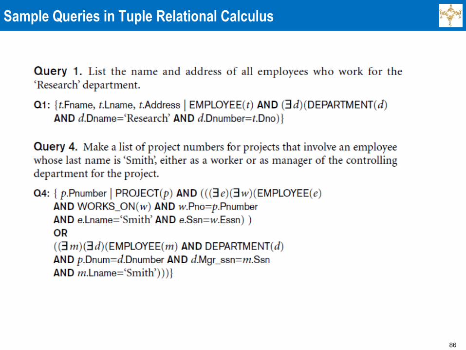
Sample Queries in Tuple Relational Calculus
87
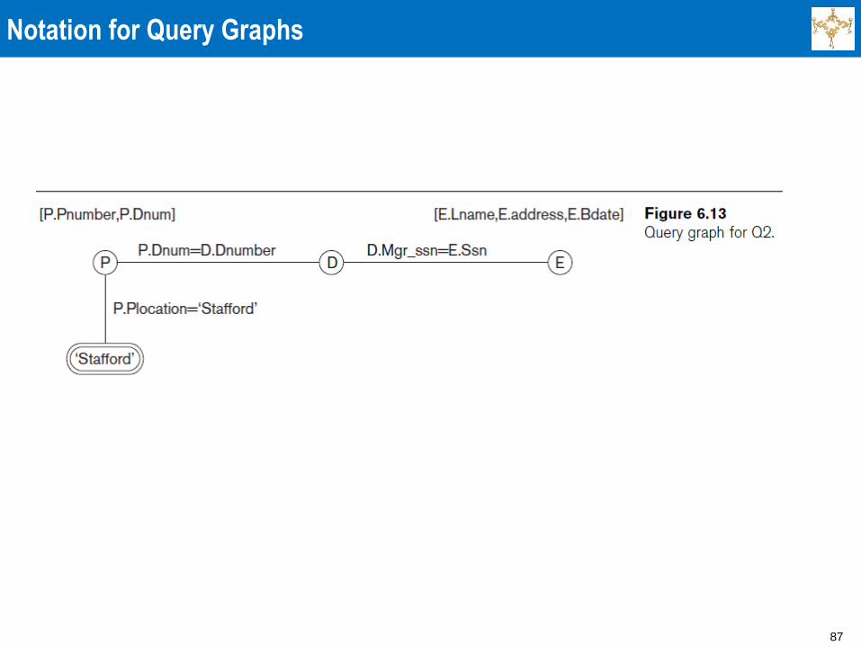
Notation for Query Graphs
88
Transforming the Universal and Existential Quantifiers
Transform one type of quantifier into other
with negation (preceded by NOT)
AND and OR replace one another
Negated formula becomes un-negated
Un-negated formula becomes negated
89
Using the Universal Quantifier in Queries
90
Safe Expressions
Guaranteed to yield a finite number of
tuples as its result
Otherwise expression is called unsafe
Expression is safe
If all values in its result are from the domain of
the expression
91
Languages Based on Tuple Relational Calculus (1/2)
The language SQL is based on tuple calculus. It uses the basic block structure to express the queries in tuple calculus:
» SELECT <list of attributes>
» FROM <list of relations>
» WHERE <conditions>
SELECT clause mentions the attributes being projected, the FROM clause mentions the relations needed in the query, and the WHERE clause mentions the selection as well as the join conditions.
» SQL syntax is expanded further to accommodate other operations. (See Textbook Chapter 8).
92
Languages Based on Tuple Relational Calculus (2/2)
Another language which is based on tuple calculus is
QUEL which actually uses the range variables as in tuple
calculus. Its syntax includes:
» RANGE OF <variable name> IS <relation name>
Then it uses
» RETRIEVE <list of attributes from range variables>
» WHERE <conditions>
This language was proposed in the relational DBMS
INGRES. (system is currently still supported by Computer
Associates – but the QUEL language is no longer there).
93
The Domain Relational Calculus (1/2)
Another variation of relational calculus called the domain relational calculus, or simply, domain calculus is equivalent to tuple calculus and to relational algebra.
The language called QBE (Query-By-Example) that is related to domain calculus was developed almost concurrently to SQL at IBM Research, Yorktown Heights, New York.
» Domain calculus was thought of as a way to explain what QBE does.
Domain calculus differs from tuple calculus in the type of variables used in formulas:
» Rather than having variables range over tuples, the variables range over single values from domains of attributes.
To form a relation of degree n for a query result, we must have n of these domain variables— one for each attribute.
94
The Domain Relational Calculus (2/2)
An expression of the domain calculus is of
the form
{ x1, x2, . . ., xn |
COND(x1, x2, . . ., xn, xn+1, xn+2, . . ., xn+m)}
» where x1, x2, . . ., xn, xn+1, xn+2, . . ., xn+m are
domain variables that range over domains (of
attributes)
» and COND is a condition or formula of the
domain relational calculus.
95
Example Query Using Domain Calculus
Retrieve the birthdate and address of the employee whose name is ‘John B. Smith’.
Query :
{uv | ( q) ( r) ( s) ( t) ( w) ( x) ( y) ( z)
(EMPLOYEE(qrstuvwxyz) and q=’John’ and r=’B’ and s=’Smith’)}
Abbreviated notation EMPLOYEE(qrstuvwxyz) uses the
variables without the separating commas: EMPLOYEE(q,r,s,t,u,v,w,x,y,z)
Ten variables for the employee relation are needed, one to range over the domain of each attribute in order.
» Of the ten variables q, r, s, . . ., z, only u and v are free.
Specify the requested attributes, BDATE and ADDRESS, by the free domain variables u for BDATE and v for ADDRESS.
Specify the condition for selecting a tuple following the bar ( | )—
» namely, that the sequence of values assigned to the variables qrstuvwxyz be a tuple of the employee relation and that the values for q (FNAME), r (MINIT), and s (LNAME) be ‘John’, ‘B’, and ‘Smith’, respectively.
96
QBE: A Query Language Based on Domain Calculus (1/2)
This language is based on the idea of giving an example
of a query using “example elements” which are nothing
but domain variables.
Notation: An example element stands for a domain
variable and is specified as an example value preceded
by the underscore character.
P. (called P dot) operator (for “print”) is placed in those
columns which are requested for the result of the query.
A user may initially start giving actual values as examples,
but later can get used to providing a minimum number of
variables as example elements.
See Textbook Appendix C
97
QBE: A Query Language Based on Domain Calculus (2/2)
The language is very user-friendly, because it uses minimal syntax.
QBE was fully developed further with facilities for grouping, aggregation, updating etc. and is shown to be equivalent to SQL.
The language is available under QMF (Query Management Facility) of DB2 of IBM and has been used in various ways by other products like ACCESS of Microsoft, and PARADOX.
For details, see Appendix C in the textbook.
98
QBE Examples
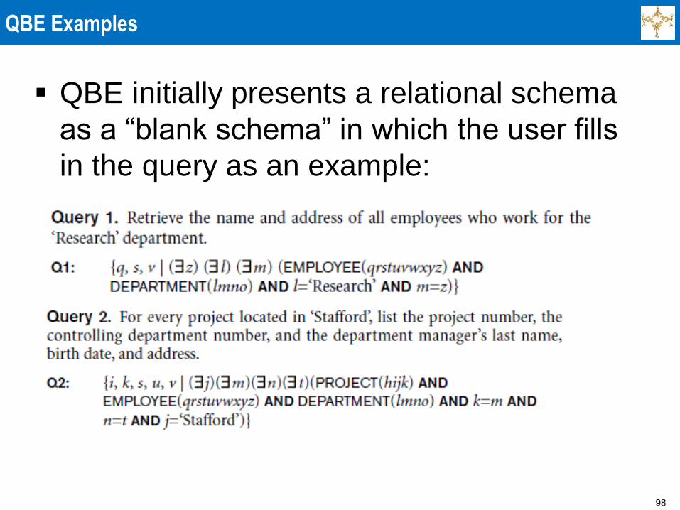
QBE initially presents a relational schema
as a “blank schema” in which the user fills
in the query as an example:
99
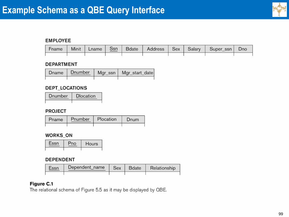
Example Schema as a QBE Query Interface
100
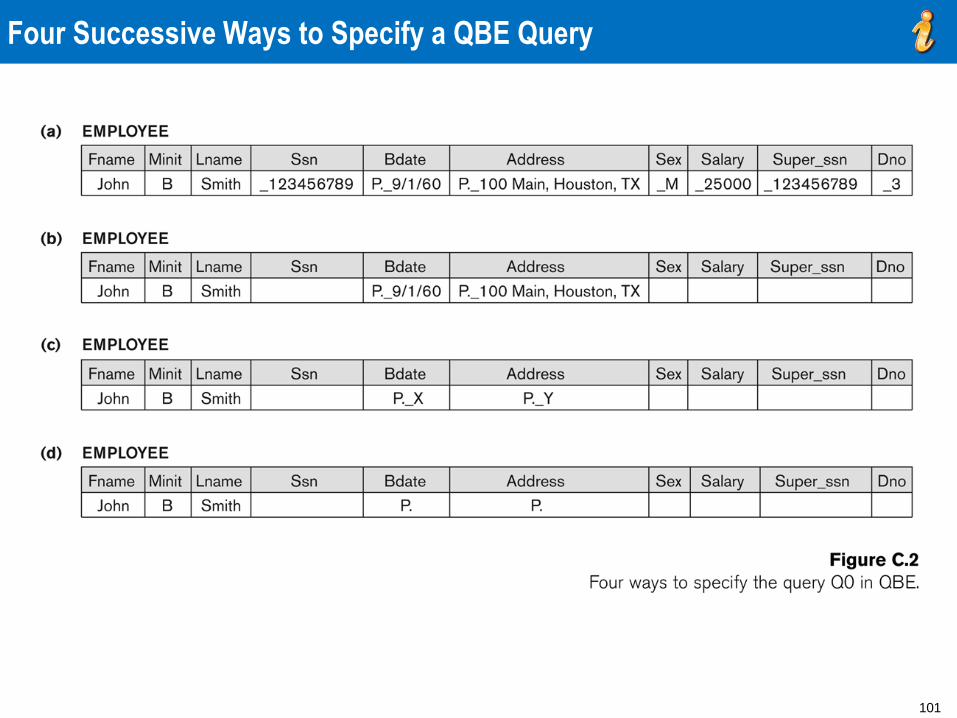
QBE Examples
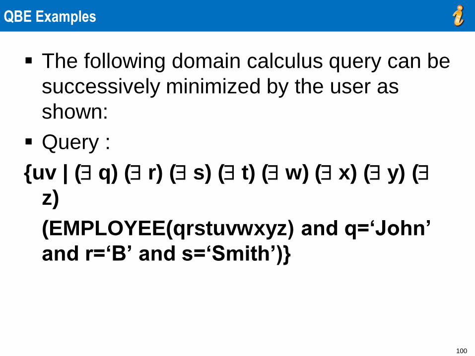
The following domain calculus query can be
successively minimized by the user as
shown:
Query :
{uv | ( q) ( r) ( s) ( t) ( w) ( x) ( y) (
z)
(EMPLOYEE(qrstuvwxyz) and q=‘John’
and r=‘B’ and s=‘Smith’)}
101
Four Successive Ways to Specify a QBE Query
102
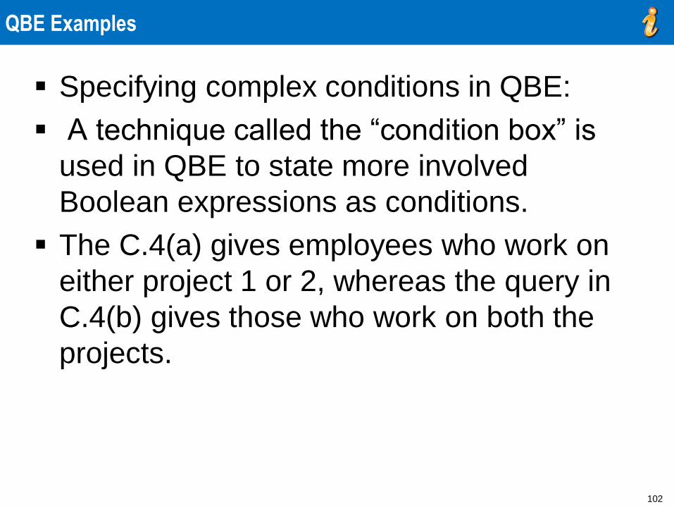
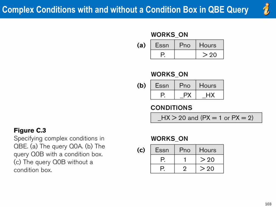
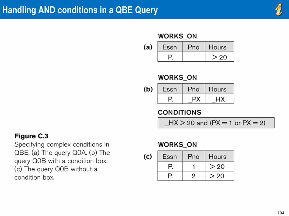
QBE Examples
Specifying complex conditions in QBE:
A technique called the “condition box” is
used in QBE to state more involved
Boolean expressions as conditions.
The C.4(a) gives employees who work on
either project 1 or 2, whereas the query in
C.4(b) gives those who work on both the
projects.
103
Complex Conditions with and without a Condition Box in QBE Query
104
Handling AND conditions in a QBE Query
105
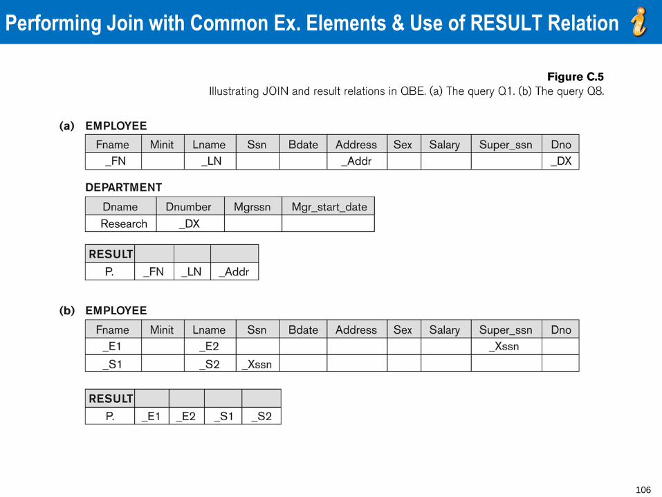
JOIN in QBE: Examples
The join is simply accomplished by using
the same example element (variable with
underscore) in the columns being joined
from different (or same as in C.5 (b))
relation.
Note that the Result is set us as an
independent table to show variables from
multiple relations placed in the result.
106
Performing Join with Common Ex. Elements & Use of RESULT Relation
107
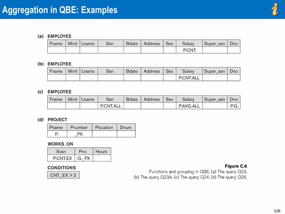
Aggregation in QBE
Aggregation is accomplished by using .CNT
for count,.MAX, .MIN, .AVG for the
corresponding aggregation functions
Grouping is accomplished by .G operator.
Condition Box may use conditions on
groups (similar to HAVING clause in SQL –
see Textbook Section 8.5.8)
108
Aggregation in QBE: Examples
109
Negation in QBE: Examples
110
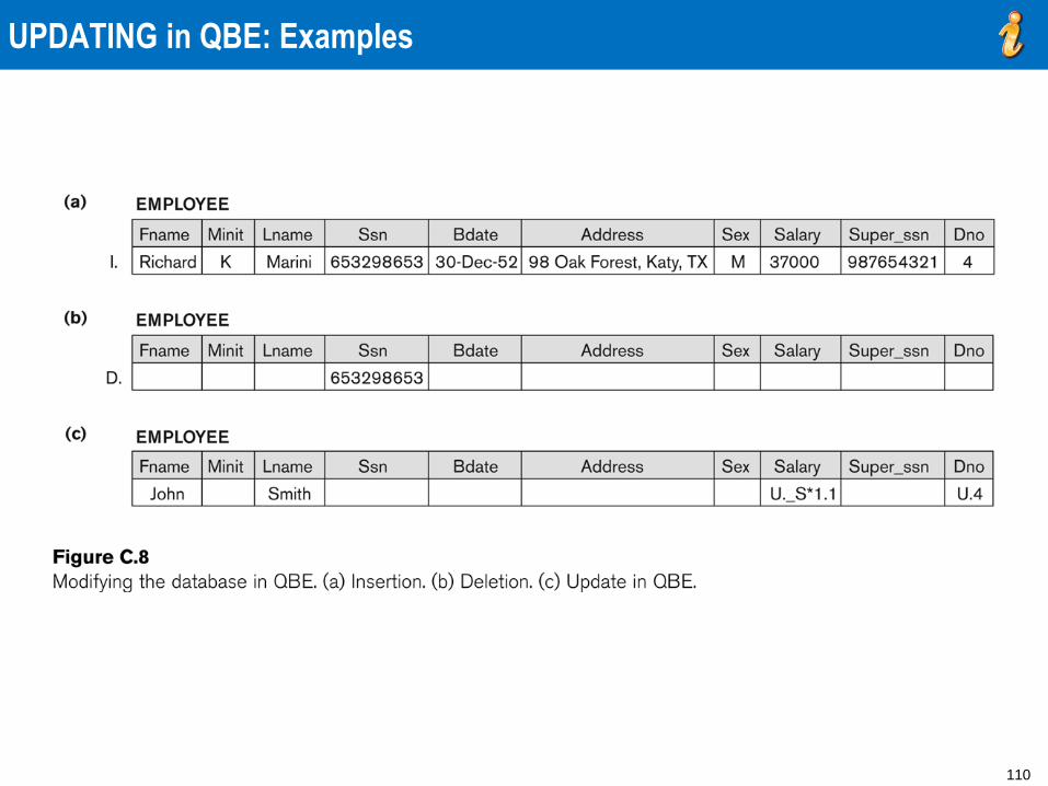
UPDATING in QBE: Examples
111
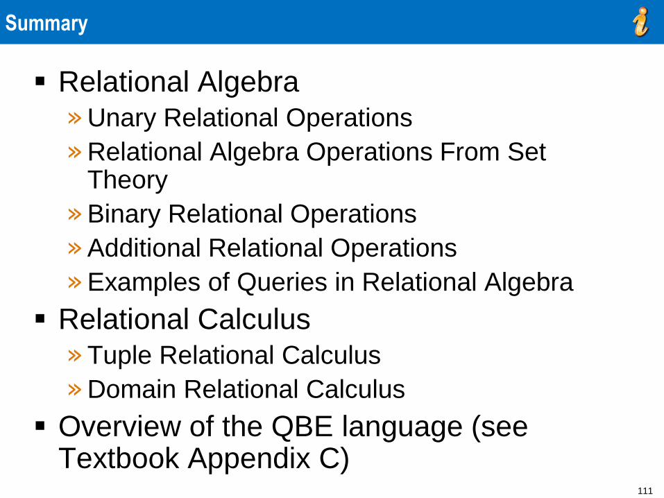
Summary
Relational Algebra
» Unary Relational Operations
» Relational Algebra Operations From Set Theory
» Binary Relational Operations
» Additional Relational Operations
» Examples of Queries in Relational Algebra
Relational Calculus
» Tuple Relational Calculus
» Domain Relational Calculus
Overview of the QBE language (see Textbook Appendix C)
112
Agenda
1 Session Overview
4 Summary and Conclusion
2 Relational Algebra and Relational Calculus
3 Relational Algebra Using SQL Syntax
113
Agenda
Relational Algebra and SQL
Basic Syntax Comparison
Sets and Operations on Relations
Relations in Relational Algebra
Empty Relations
Relational Algebra vs. Full SQL
Operations on Relations
» Projection
» Selection
» Cartesian Product
» Union
» Difference
» Intersection
From Relational Algebra to Queries (with Examples)
Microsoft Access Case Study
Pure Relational Algebra
114
Relational Algebra And SQL
SQL is based on relational algebra with many extensions
» Some necessary
» Some unnecessary
“Pure” relational algebra, use mathematical notation with Greek
letters
It is covered here using SQL syntax; that is this unit covers
relational algebra, but it looks like SQL
And will be really valid SQL
Pure relational algebra is used in research, scientific papers, and
some textbooks
So it is good to know it, and material is provided at the end of this
unit material from which one can learn it
But in anything practical, including commercial systems, you will be
using SQL
115
Key Differences Between SQL And “Pure” Relational Algebra
SQL data model is a multiset not a set; still rows in tables (we
sometimes continue calling relations)
» Still no order among rows: no such thing as 1st row
» We can (if we want to) count how many times a particular row appears
in the table
» We can remove/not remove duplicates as we specify (most of the time)
» There are some operators that specifically pay attention to duplicates
» We must know whether duplicates are removed (and how) for each
SQL operation; luckily, easy
Many redundant operators (relational algebra had only one:
intersection)
SQL provides statistical operators, such as AVG (average)
» Can be performed on subsets of rows; e.g. average salary per
company branch
116
Key Differences Between Relational Algebra And SQL
Every domain is “enhanced” with a special
element: NULL
» Very strange semantics for handling these
elements
“Pretty printing” of output: sorting, and
similar
Operations for
» Inserting
» Deleting
» Changing/updating (sometimes not easily
reducible to deleting and inserting)
117
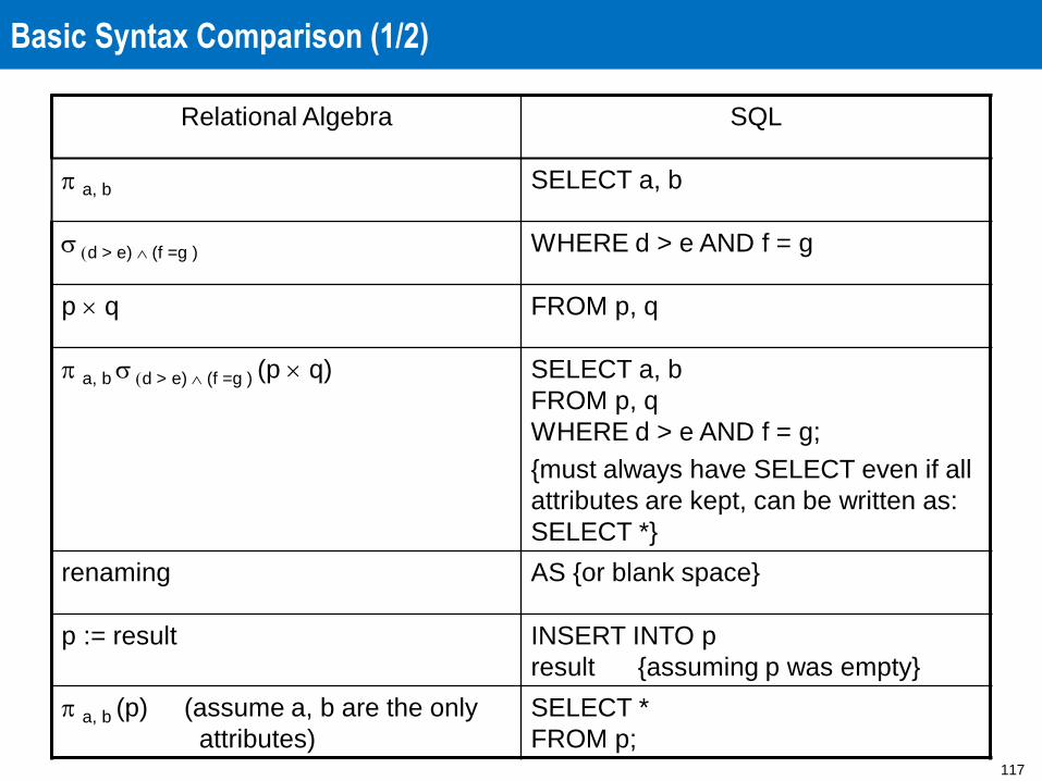
Basic Syntax Comparison (1/2)
Relational Algebra SQL
a, b SELECT a, b
(d > e) (f =g ) WHERE d > e AND f = g
p q FROM p, q
a, b (d > e) (f =g ) (p q) SELECT a, b
FROM p, q
WHERE d > e AND f = g;
{must always have SELECT even if all
attributes are kept, can be written as:
SELECT *}
renaming AS {or blank space}
p := result INSERT INTO p
result {assuming p was empty}
a, b (p) (assume a, b are the only
attributes)
SELECT *
FROM p;
118
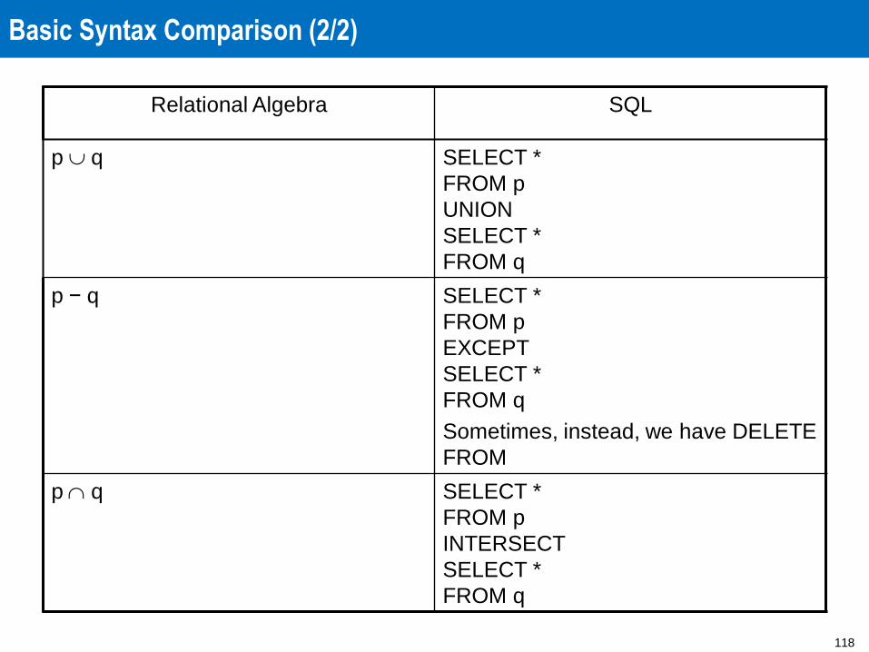
Basic Syntax Comparison (2/2)
Relational Algebra SQL
p q SELECT *
FROM p
UNION
SELECT *
FROM q
p − q SELECT *
FROM p
EXCEPT
SELECT *
FROM q
Sometimes, instead, we have DELETE
FROM
p q SELECT *
FROM p
INTERSECT
SELECT *
FROM q
119
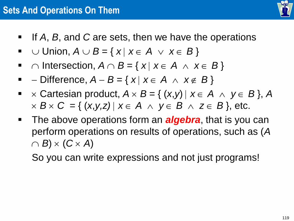
Sets And Operations On Them
If A, B, and C are sets, then we have the operations
Union, A B = { x x A x B }
Intersection, A B = { x x A x B }
- Difference, A - B = { x x A x B }
Cartesian product, A B = { (x,y) x A y B }, A
B C = { (x,y,z) x A y B z B }, etc.
The above operations form an algebra, that is you can
perform operations on results of operations, such as (A
B) (C A)
So you can write expressions and not just programs!
120
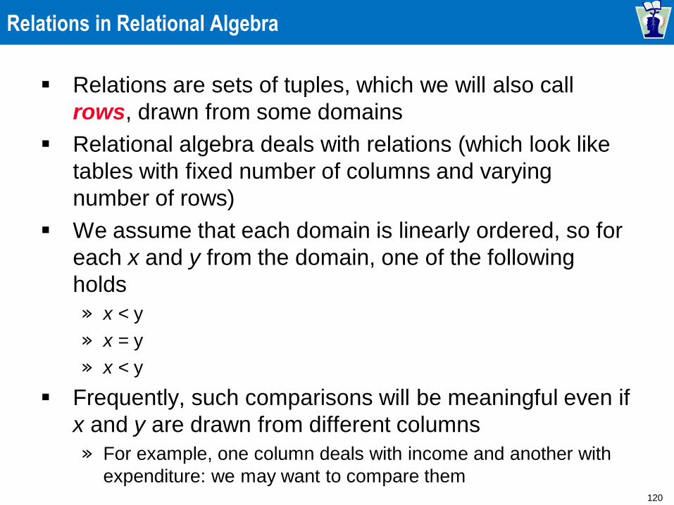
Relations in Relational Algebra
Relations are sets of tuples, which we will also call
rows, drawn from some domains
Relational algebra deals with relations (which look like
tables with fixed number of columns and varying
number of rows)
We assume that each domain is linearly ordered, so for
each x and y from the domain, one of the following
holds
» x < y
» x = y
» x < y
Frequently, such comparisons will be meaningful even if
x and y are drawn from different columns
» For example, one column deals with income and another with
expenditure: we may want to compare them
121
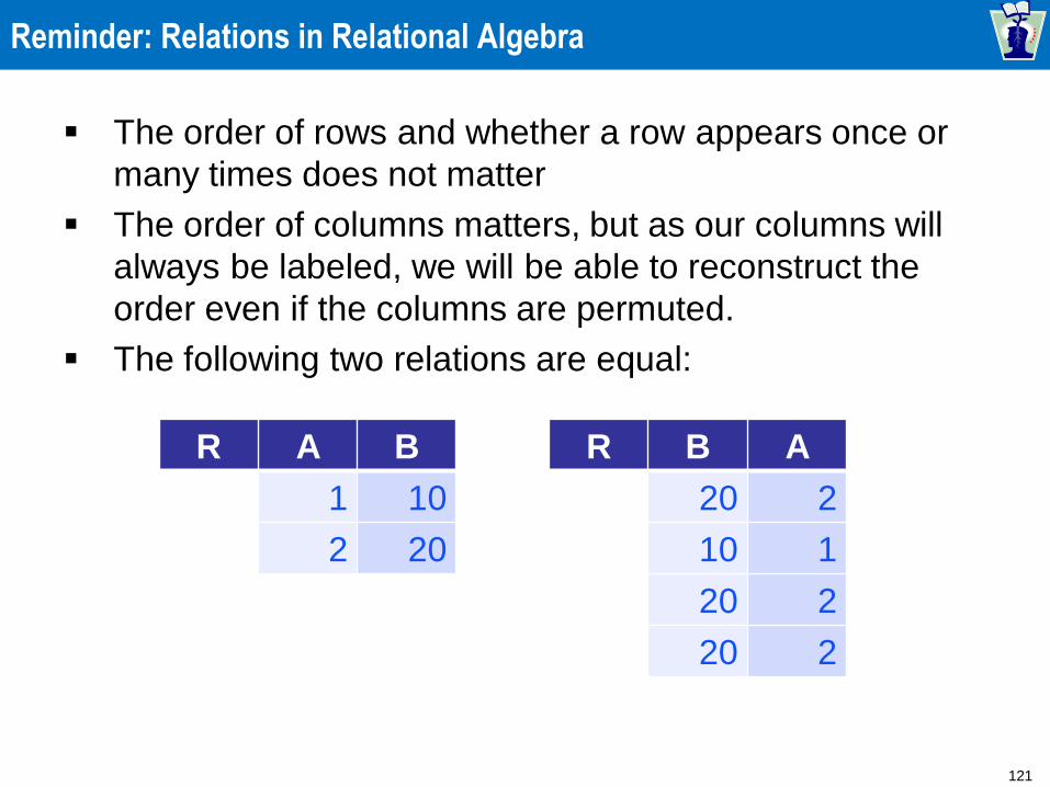
Reminder: Relations in Relational Algebra
The order of rows and whether a row appears once or
many times does not matter
The order of columns matters, but as our columns will
always be labeled, we will be able to reconstruct the
order even if the columns are permuted.
The following two relations are equal:
R A B
1 10
2 20
R B A
20 2
10 1
20 2
20 2
122
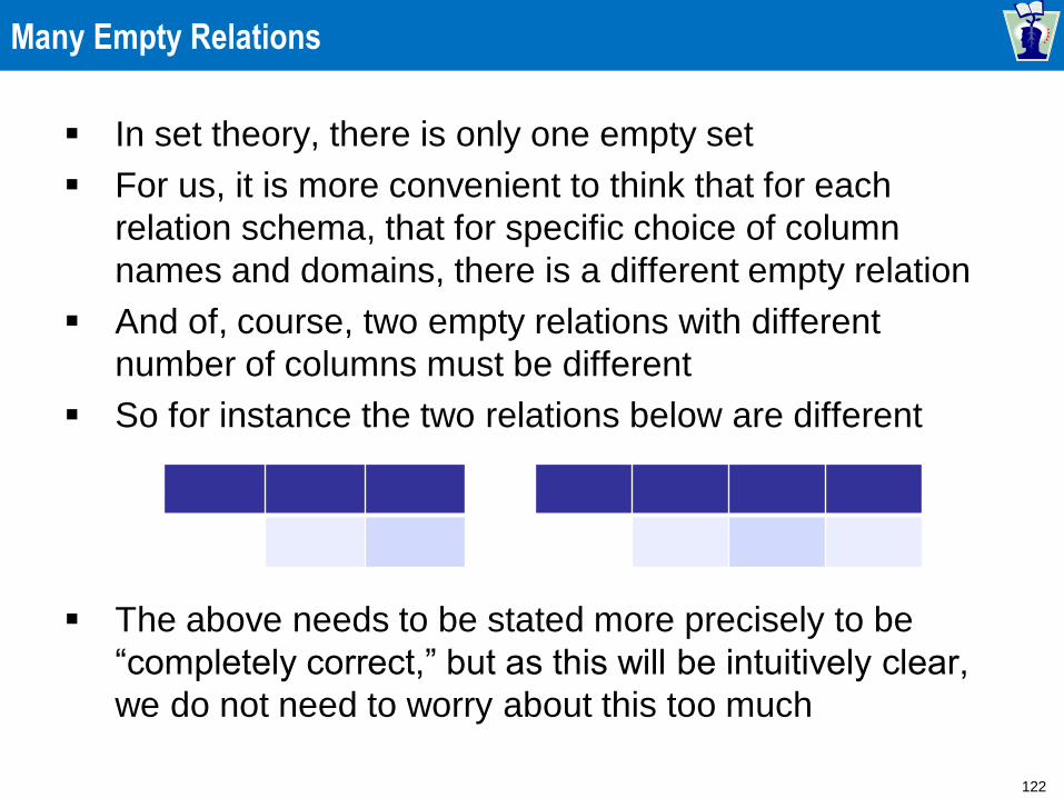
Many Empty Relations
In set theory, there is only one empty set
For us, it is more convenient to think that for each
relation schema, that for specific choice of column
names and domains, there is a different empty relation
And of, course, two empty relations with different
number of columns must be different
So for instance the two relations below are different
The above needs to be stated more precisely to be
“completely correct,” but as this will be intuitively clear,
we do not need to worry about this too much
123
Relational Algebra Versus Full SQL
Relational algebra is restricted to querying the database
Does not have support for
» Primary keys
» Foreign keys
» Inserting data
» Deleting data
» Updating data
» Indexing
» Recovery
» Concurrency
» Security
» …
Does not care about efficiency, only about specifications
of what is needed
124
Operations on relations
There are several fundamental operations on
relations
We will describe them in turn:
» Projection
» Selection
» Cartesian product
» Union
» Difference
» Intersection (technically not fundamental)
The very important property: Any operation on
relations produces a relation
This is why we call this an algebra
125
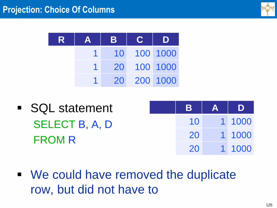
Projection: Choice Of Columns
SQL statement
SELECT B, A, D
FROM R
We could have removed the duplicate
row, but did not have to
R A B C D
1 10 100 1000
1 20 100 1000
1 20 200 1000
B A D
10 1 1000
20 1 1000
20 1 1000
126
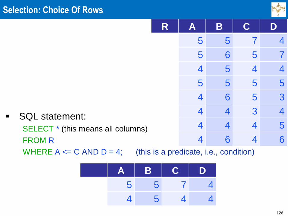
Selection: Choice Of Rows
SQL statement:
SELECT * (this means all columns)
FROM R
WHERE A <= C AND D = 4; (this is a predicate, i.e., condition)
R A B C D
5 5 7 4
5 6 5 7
4 5 4 4
5 5 5 5
4 6 5 3
4 4 3 4
4 4 4 5
4 6 4 6
A B C D
5 5 7 4
4 5 4 4
127
Selection
In general, the condition (predicate) can be
specified by a Boolean formula with
NOT, AND, OR on atomic conditions, where a
condition is:
» a comparison between two column names,
» a comparison between a column name and a
constant
» Technically, a constant should be put in quotes
» Even a number, such as 4, perhaps should be put in
quotes, as ‘4’, so that it is distinguished from a
column name, but as we will never use numbers for
column names, this not necessary
128
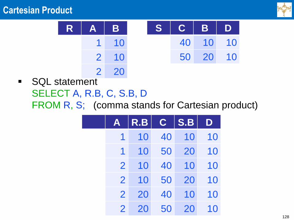
Cartesian Product
SQL statement
SELECT A, R.B, C, S.B, D
FROM R, S; (comma stands for Cartesian product)
A R.B C S.B D
1 10 40 10 10
1 10 50 20 10
2 10 40 10 10
2 10 50 20 10
2 20 40 10 10
2 20 50 20 10
R A B
1 10
2 10
2 20
S C B D
40 10 10
50 20 10
129
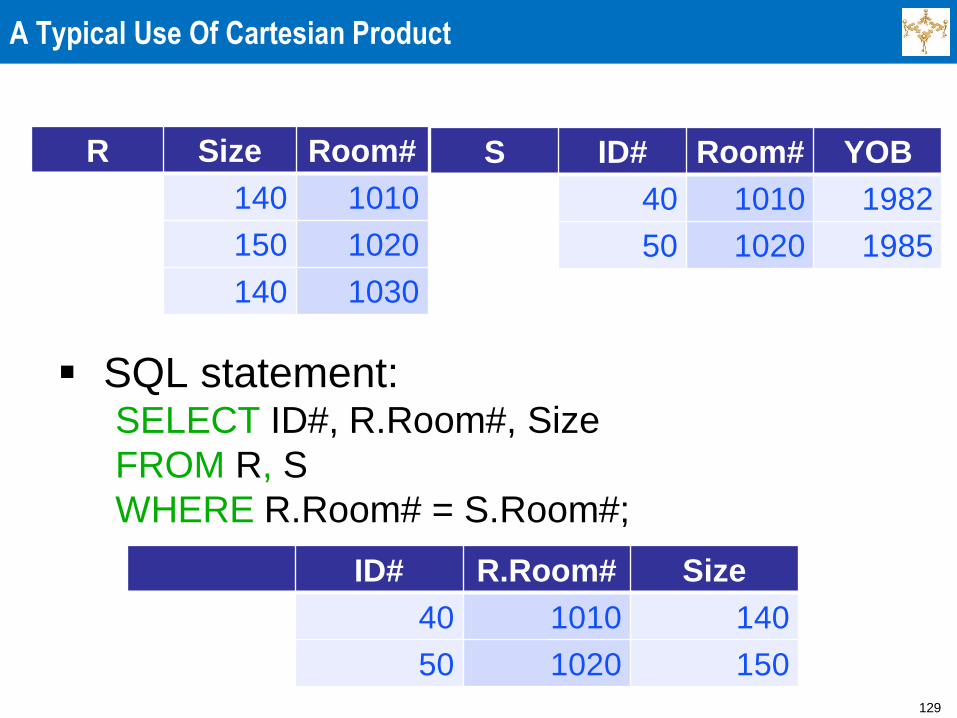
A Typical Use Of Cartesian Product
SQL statement: SELECT ID#, R.Room#, Size
FROM R, S
WHERE R.Room# = S.Room#;
R Size Room#
140 1010
150 1020
140 1030
S ID# Room# YOB
40 1010 1982
50 1020 1985
ID# R.Room# Size
40 1010 140
50 1020 150
130
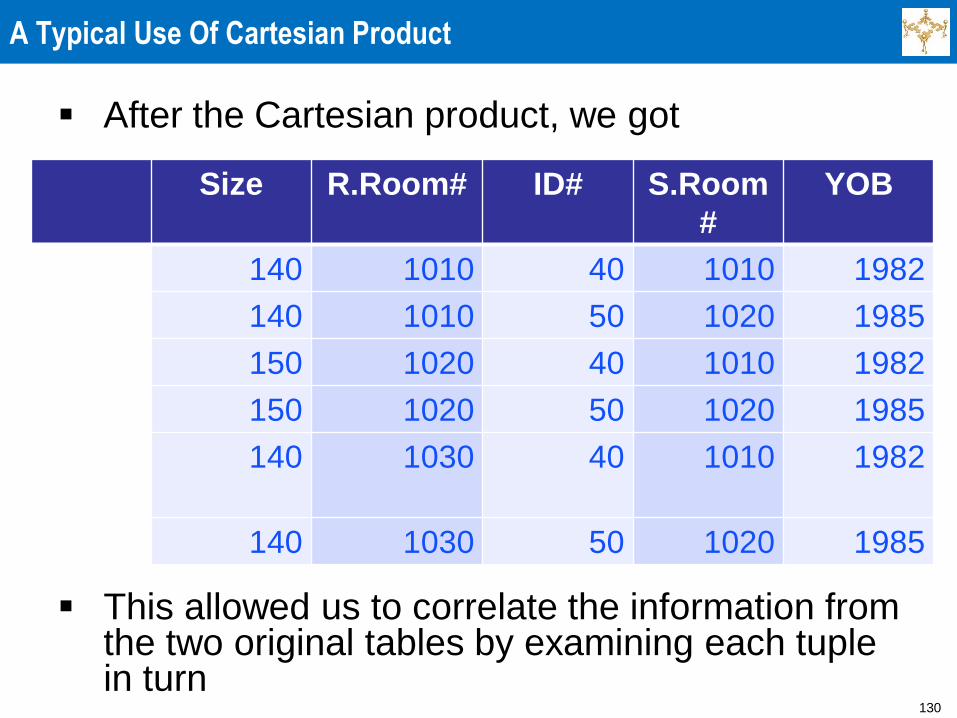
A Typical Use Of Cartesian Product
After the Cartesian product, we got
This allowed us to correlate the information from the two original tables by examining each tuple in turn
Size R.Room# ID# S.Room
#
YOB
140 1010 40 1010 1982
140 1010 50 1020 1985
150 1020 40 1010 1982
150 1020 50 1020 1985
140 1030 40 1010 1982
140 1030 50 1020 1985
131
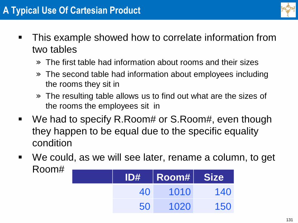
A Typical Use Of Cartesian Product
This example showed how to correlate information from
two tables
» The first table had information about rooms and their sizes
» The second table had information about employees including
the rooms they sit in
» The resulting table allows us to find out what are the sizes of
the rooms the employees sit in
We had to specify R.Room# or S.Room#, even though
they happen to be equal due to the specific equality
condition
We could, as we will see later, rename a column, to get
Room# ID# Room# Size
40 1010 140
50 1020 150
132
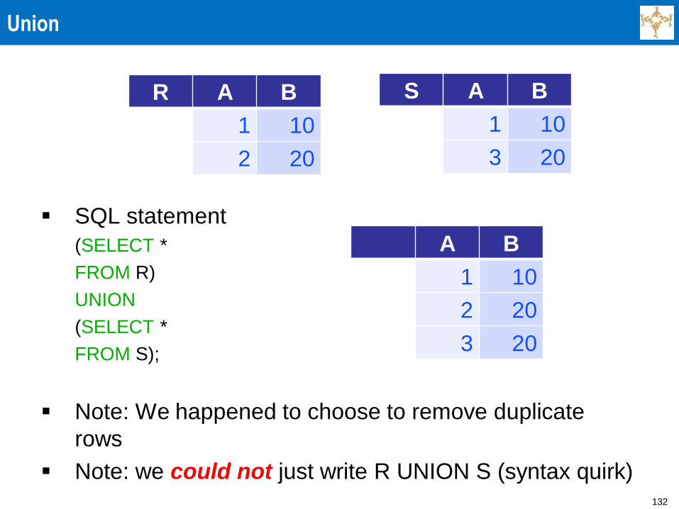
Union
SQL statement
(SELECT *
FROM R)
UNION
(SELECT *
FROM S);
Note: We happened to choose to remove duplicate
rows
Note: we could not just write R UNION S (syntax quirk)
R A B
1 10
2 20
S A B
1 10
3 20
A B
1 10
2 20
3 20
133
Union Compatibility
We require same -arity (number of columns),
otherwise the result is not a relation
Also, the operation “probably” should make
sense, that is the values in corresponding
columns should be drawn from the same
domains
Actually, best to assume that the column names
are the same and that is what we will do from
now on
We refer to these as union compatibility of
relations
Sometimes, just the term compatibility is used
134
Difference
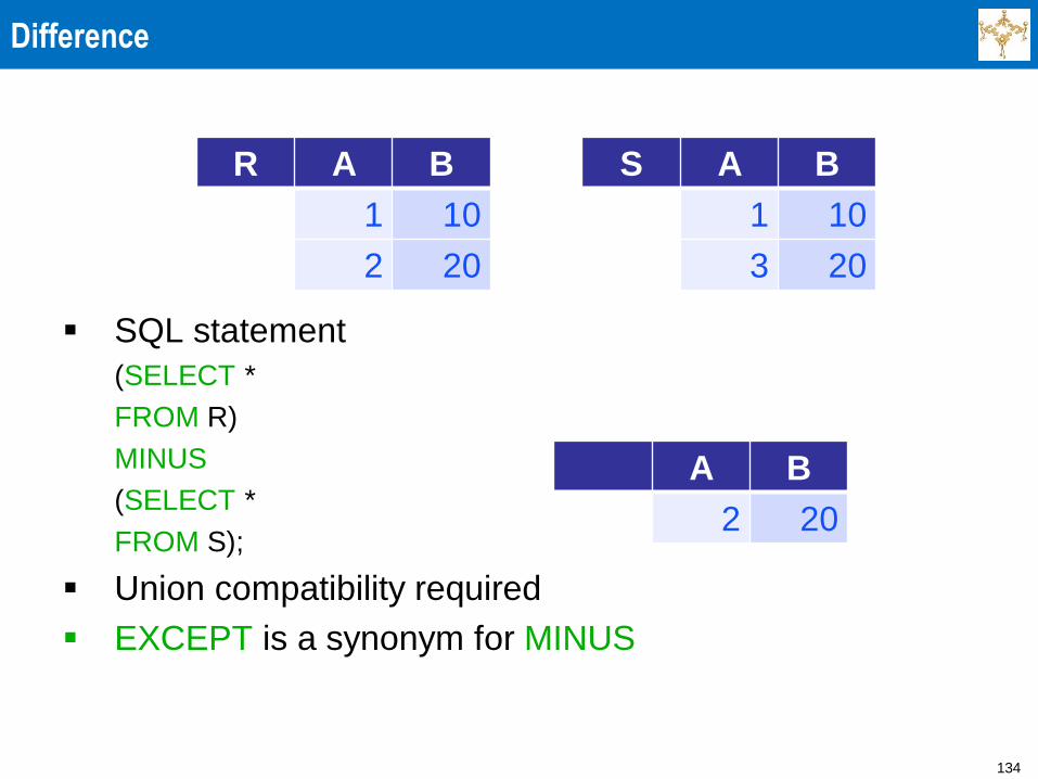
SQL statement
(SELECT *
FROM R)
MINUS
(SELECT *
FROM S);
Union compatibility required
EXCEPT is a synonym for MINUS
R A B
1 10
2 20
S A B
1 10
3 20
A B
2 20
135
Intersection
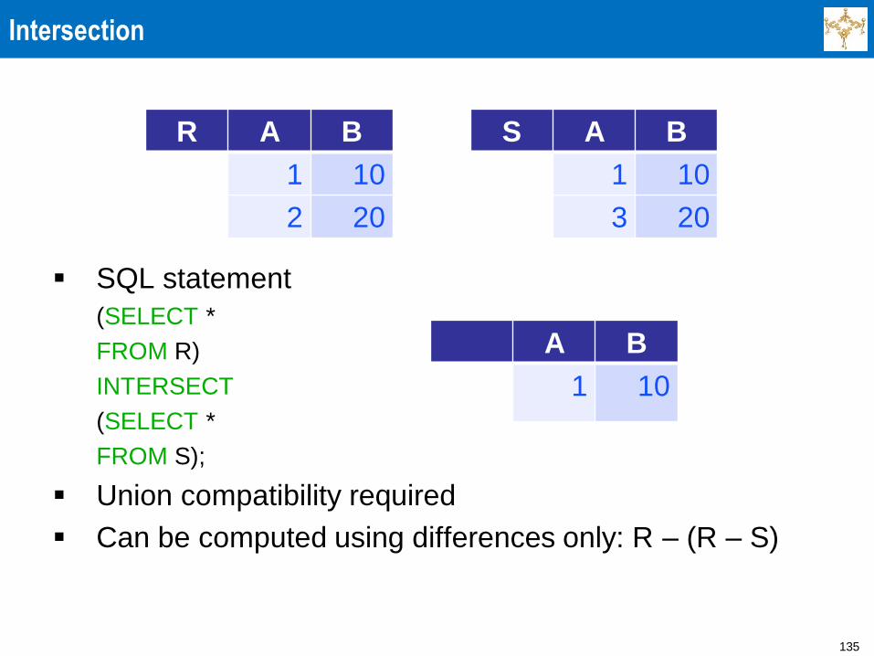
SQL statement
(SELECT *
FROM R)
INTERSECT
(SELECT *
FROM S);
Union compatibility required
Can be computed using differences only: R – (R – S)
R A B
1 10
2 20
S A B
1 10
3 20
A B
1 10
136
From Relational Algebra to Queries
These operations allow us to define a large
number of interesting queries for relational
databases.
In order to be able to formulate our examples,
we will assume standard programming
language type of operations:
» Assignment of an expression to a new variable;
In our case assignment of a relational expression to
a relational variable.
» Renaming of a relations, to use another name to
denote it
» Renaming of a column, to use another name to
denote it
137
A Small Example
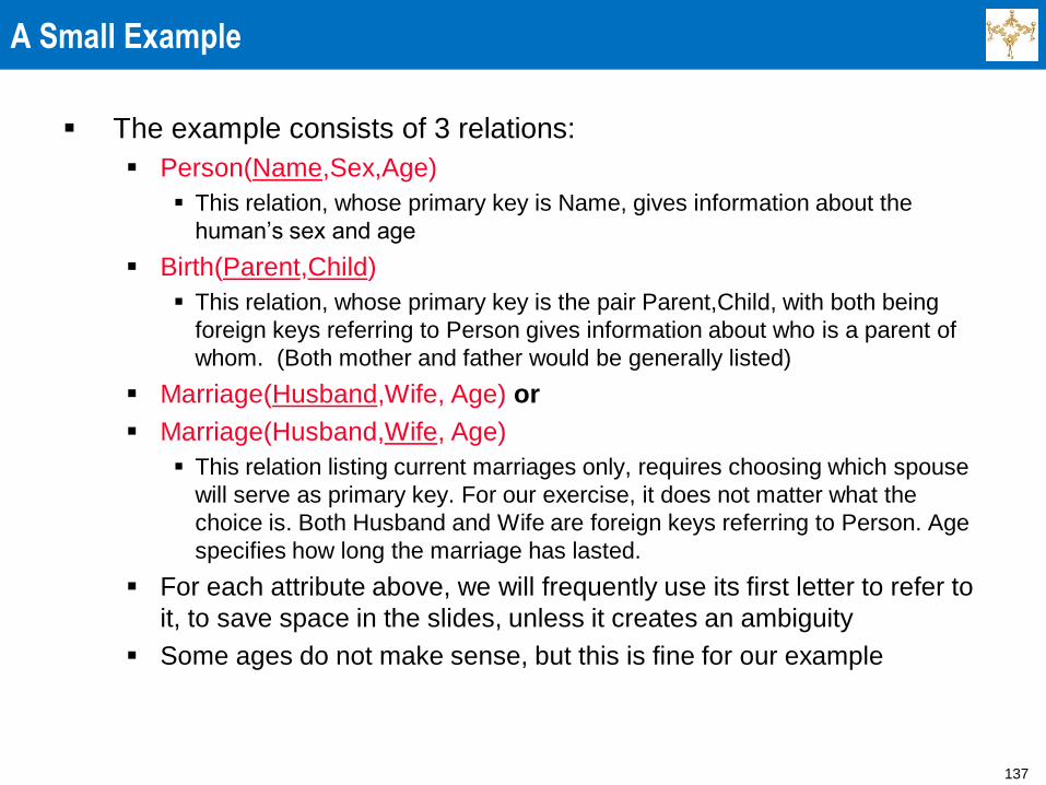
The example consists of 3 relations:
Person(Name,Sex,Age)
This relation, whose primary key is Name, gives information about the
human’s sex and age
Birth(Parent,Child)
This relation, whose primary key is the pair Parent,Child, with both being
foreign keys referring to Person gives information about who is a parent of
whom. (Both mother and father would be generally listed)
Marriage(Husband,Wife, Age) or
Marriage(Husband,Wife, Age)
This relation listing current marriages only, requires choosing which spouse
will serve as primary key. For our exercise, it does not matter what the
choice is. Both Husband and Wife are foreign keys referring to Person. Age
specifies how long the marriage has lasted.
For each attribute above, we will frequently use its first letter to refer to
it, to save space in the slides, unless it creates an ambiguity
Some ages do not make sense, but this is fine for our example
138
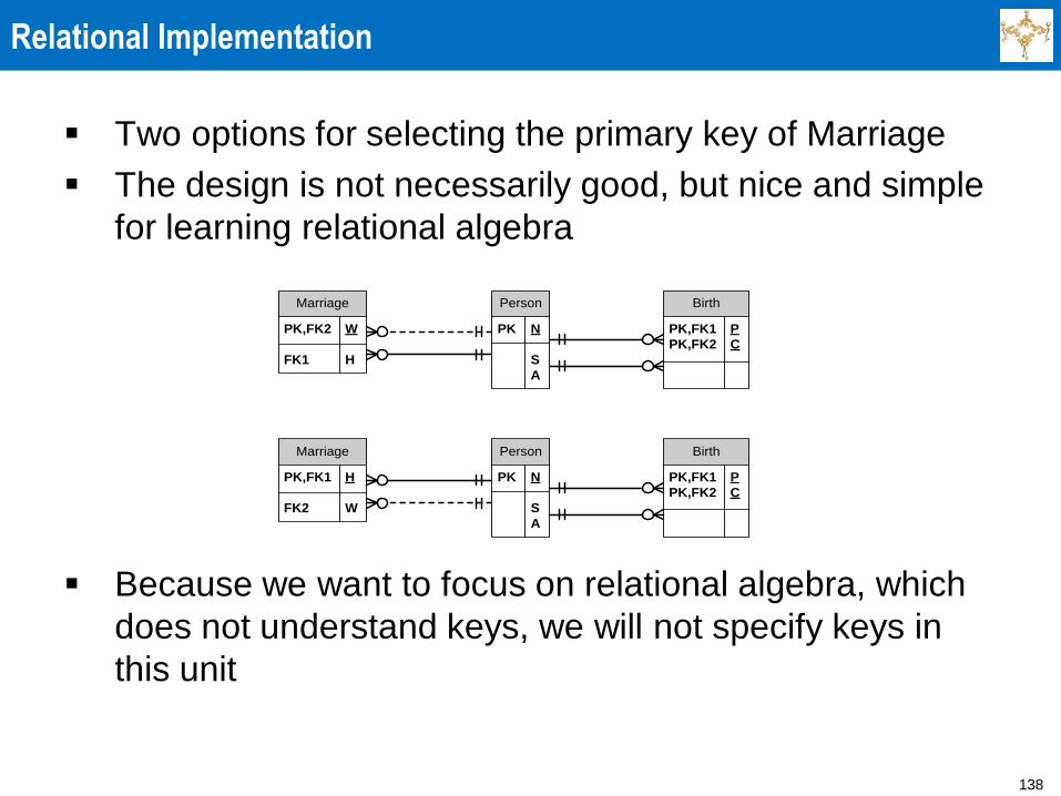
Relational Implementation
Two options for selecting the primary key of Marriage
The design is not necessarily good, but nice and simple
for learning relational algebra
Because we want to focus on relational algebra, which
does not understand keys, we will not specify keys in
this unit
Marriage
PK,FK2 W
FK1 H
Person
PK N
S
A
Birth
PK,FK1 P
PK,FK2 C
Marriage
PK,FK1 H
FK2 W
Person
PK N
S
A
Birth
PK,FK1 P
PK,FK2 C
139
Microsoft Access Database
Microsoft Access Database with this example
has been posted
» The example suggests that you download and install
Microsoft Access 2007
» The examples are in the Access 2000 format so that
if you have an older version, you can work with it
Access is a very good tool for quickly learning
basic constructs of SQL DML, although it is not
suitable for anything other than personal
databases
140
Microsoft Access Database
The database and our queries (other than the one with
MINUS at the end) are the appropriate “extras” directory
on the class web in “slides”
» MINUS is frequently specified in commercial databases in a
roundabout way
» We will cover how it is done when we discuss commercial
databases
Our sample Access database: People.mdb
The queries in Microsoft Access are copied and pasted
in these notes, after reformatting them
Included copied and pasted screen shots of the results
of the queries so that you can correlate the queries with
the names of the resulting tables

141
Our Database With Sample Queries - Open In Microsoft Access
142
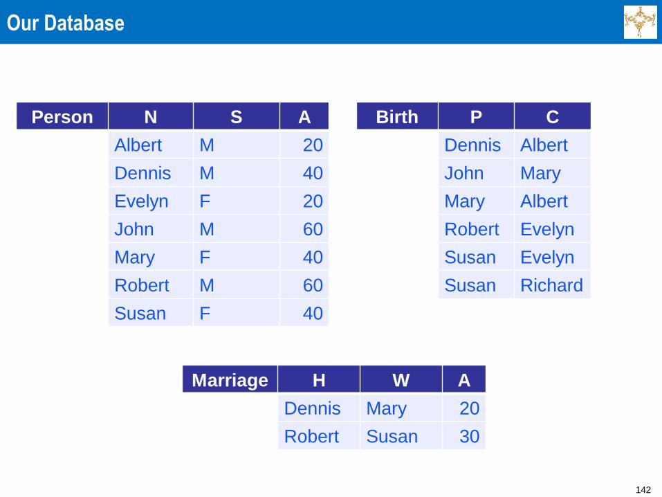
Our Database
Person N S A
Albert M 20
Dennis M 40
Evelyn F 20
John M 60
Mary F 40
Robert M 60
Susan F 40
Birth P C
Dennis Albert
John Mary
Mary Albert
Robert Evelyn
Susan Evelyn
Susan Richard
Marriage H W A
Dennis Mary 20
Robert Susan 30
143
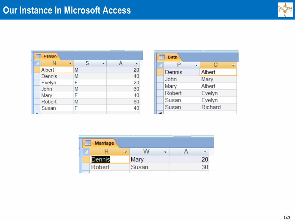
Our Instance In Microsoft Access
144
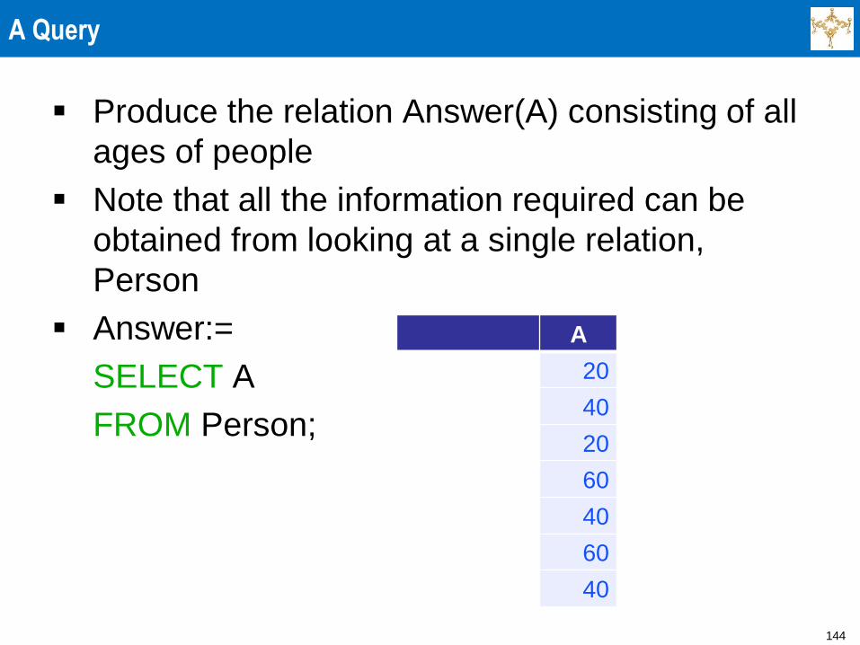
A Query
Produce the relation Answer(A) consisting of all
ages of people
Note that all the information required can be
obtained from looking at a single relation,
Person
Answer:=
SELECT A
FROM Person;
Recall that whether duplicates are removed is
not important (at least for the time being in our
course)
A
20
40
20
60
40
60
40
145
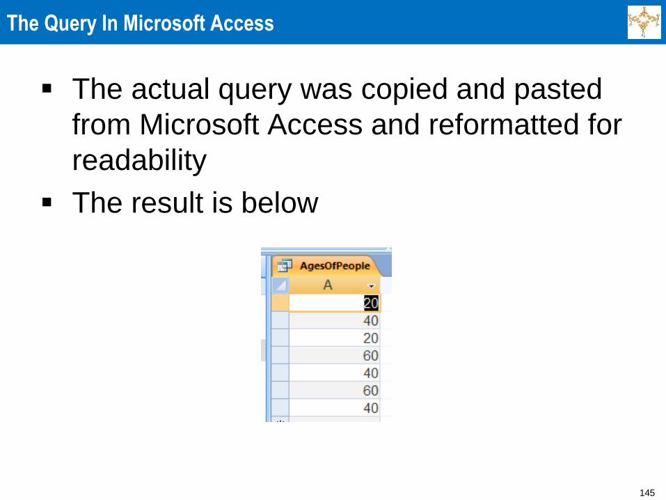
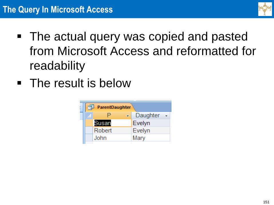
The Query In Microsoft Access
The actual query was copied and pasted
from Microsoft Access and reformatted for
readability
The result is below
146
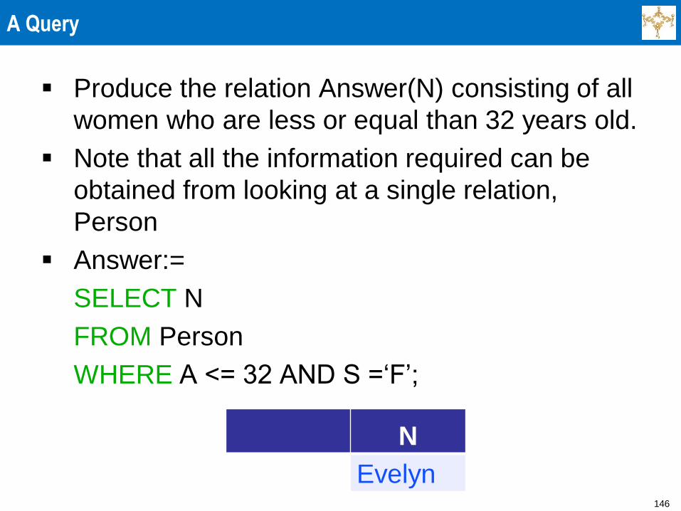
A Query
Produce the relation Answer(N) consisting of all
women who are less or equal than 32 years old.
Note that all the information required can be
obtained from looking at a single relation,
Person
Answer:=
SELECT N
FROM Person
WHERE A <= 32 AND S =‘F’;
N
Evelyn
147
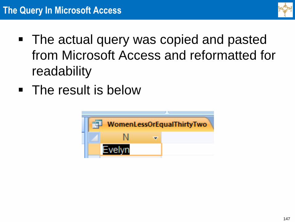
The Query In Microsoft Access
The actual query was copied and pasted
from Microsoft Access and reformatted for
readability
The result is below
148
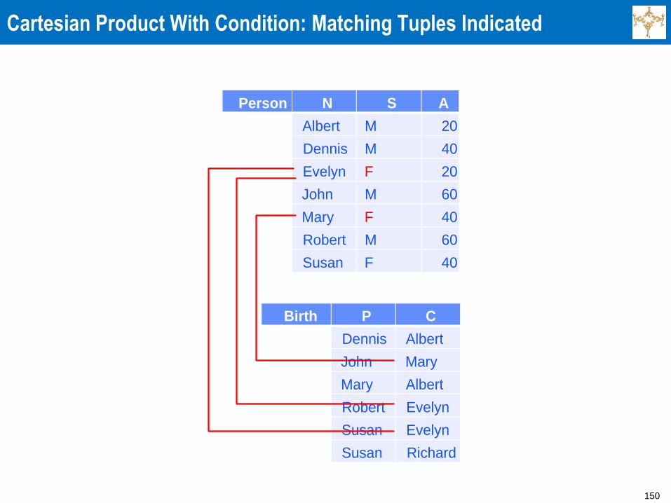
A Query
Produce a relation Answer(P, Daughter) with
the obvious meaning
Here, even though the answer comes only from
the single relation Birth, we still have to check in
the relation Person what the S of the C is
To do that, we create the Cartesian product of
the two relations: Person and Birth. This gives
us “long tuples,” consisting of a tuple in Person
and a tuple in Birth
For our purpose, the two tuples matched if N in
Person is C in Birth and the S of the N is F
149
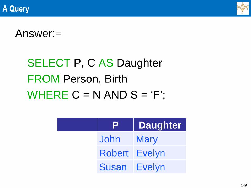
A Query
Answer:=
SELECT P, C AS Daughter
FROM Person, Birth
WHERE C = N AND S = ‘F’;
Note that AS was the attribute renaming
operator
P Daughter
John Mary
Robert Evelyn
Susan Evelyn
150
Cartesian Product With Condition: Matching Tuples Indicated
Person N S A
Albert M 20
Dennis M 40
Evelyn F 20
John M 60
Mary F 40
Robert M 60
Susan F 40
Birth P C
Dennis Albert
John Mary
Mary Albert
Robert Evelyn
Susan Evelyn
Susan Richard
151
The Query In Microsoft Access
The actual query was copied and pasted
from Microsoft Access and reformatted for
readability
The result is below
152
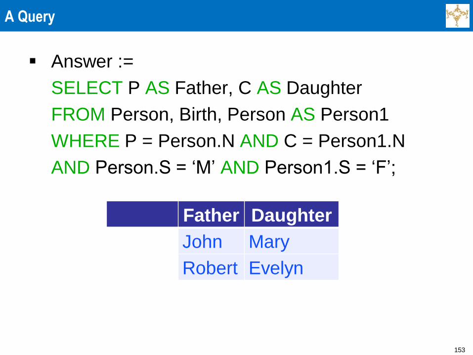
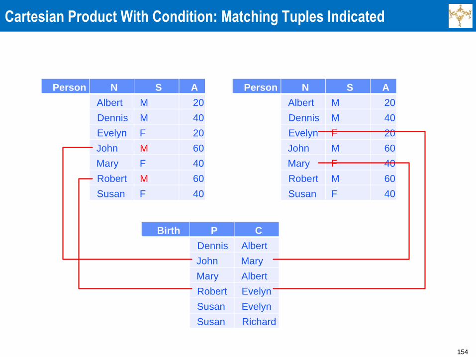
A Query
Produce a relation Answer(Father, Daughter) with the
obvious meaning.
Here we have to simultaneously look at two copies of
the relation Person, as we have to determine both the S
of the Parent and the S of the C
We need to have two distinct copies of Person in our
SQL query
But, they have to have different names so we can
specify to which we refer
Again, we use AS as a renaming operator, these time
for relations
Note: We could have used what we have already
computer: Parent,Daughter
153
A Query
Answer :=
SELECT P AS Father, C AS Daughter
FROM Person, Birth, Person AS Person1
WHERE P = Person.N AND C = Person1.N
AND Person.S = ‘M’ AND Person1.S = ‘F’;
Father Daughter
John Mary
Robert Evelyn
154
Cartesian Product With Condition: Matching Tuples Indicated
Person N S A
Albert M 20
Dennis M 40
Evelyn F 20
John M 60
Mary F 40
Robert M 60
Susan F 40
Birth P C
Dennis Albert
John Mary
Mary Albert
Robert Evelyn
Susan Evelyn
Susan Richard
Person N S A
Albert M 20
Dennis M 40
Evelyn F 20
John M 60
Mary F 40
Robert M 60
Susan F 40
155
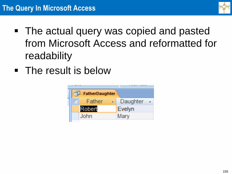
The Query In Microsoft Access
The actual query was copied and pasted
from Microsoft Access and reformatted for
readability
The result is below
156
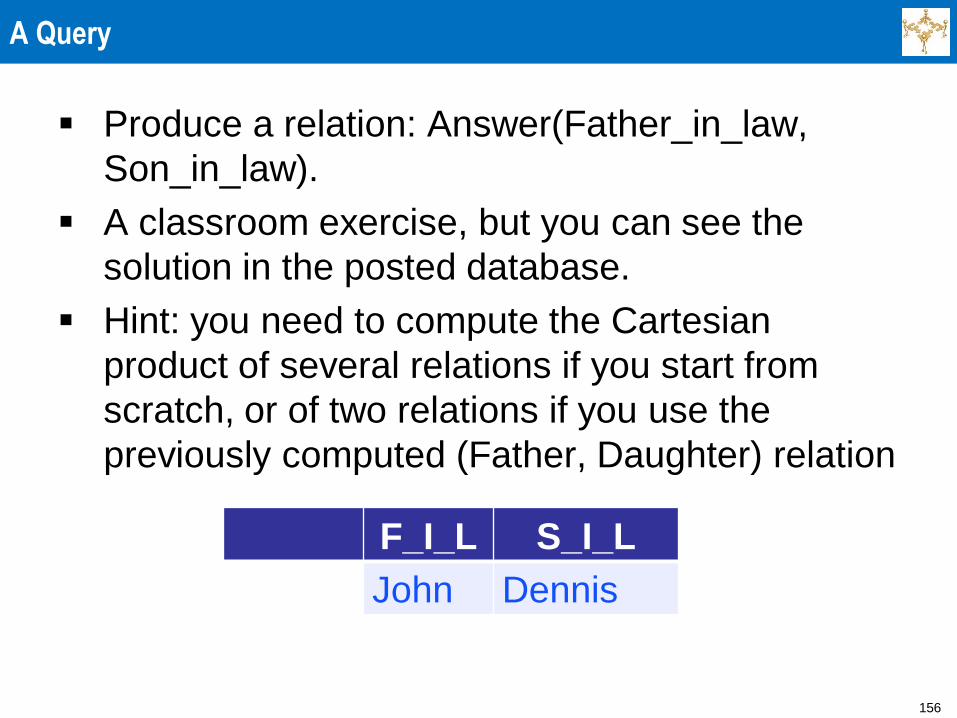
A Query
Produce a relation: Answer(Father_in_law,
Son_in_law).
A classroom exercise, but you can see the
solution in the posted database.
Hint: you need to compute the Cartesian
product of several relations if you start from
scratch, or of two relations if you use the
previously computed (Father, Daughter) relation
F_I_L S_I_L
John Dennis
157
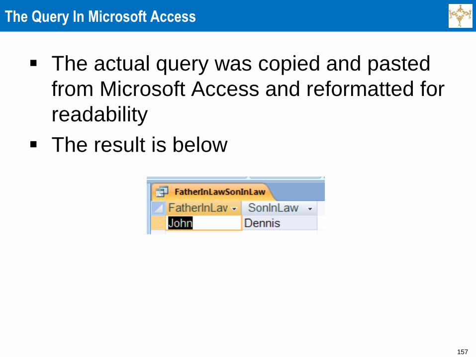
The Query In Microsoft Access
The actual query was copied and pasted
from Microsoft Access and reformatted for
readability
The result is below
158
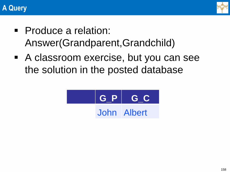
A Query
Produce a relation:
Answer(Grandparent,Grandchild)
A classroom exercise, but you can see
the solution in the posted database
G_P G_C
John Albert
159
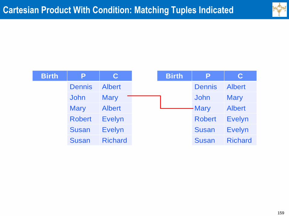
Cartesian Product With Condition: Matching Tuples Indicated
Birth P C
Dennis Albert
John Mary
Mary Albert
Robert Evelyn
Susan Evelyn
Susan Richard
Birth P C
Dennis Albert
John Mary
Mary Albert
Robert Evelyn
Susan Evelyn
Susan Richard
160
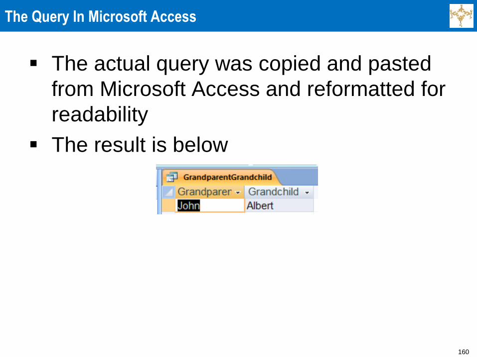
The Query In Microsoft Access
The actual query was copied and pasted
from Microsoft Access and reformatted for
readability
The result is below
161
Further Distance
How to compute (Great-grandparent,Great-grandchild)?
Easy, just take the Cartesian product of the
(Grandparent, Grandchild) table with (Parent,Child)
table and specify equality on the “intermediate” person
How to compute (Great-great-grandparent,Great-great-
grandchild)?
Easy, just take the Cartesian product of the
(Grandparent, Grandchild) table with itself and specify
equality on the “intermediate” person
Similarly, can compute (Greatx-grandparent,Greatx-
grandchild), for any x
Ultimately, may want (Ancestor,Descendant)
162
Relational Algebra Is Not Universal:Cannot Compute (Ancestor,Descendant)
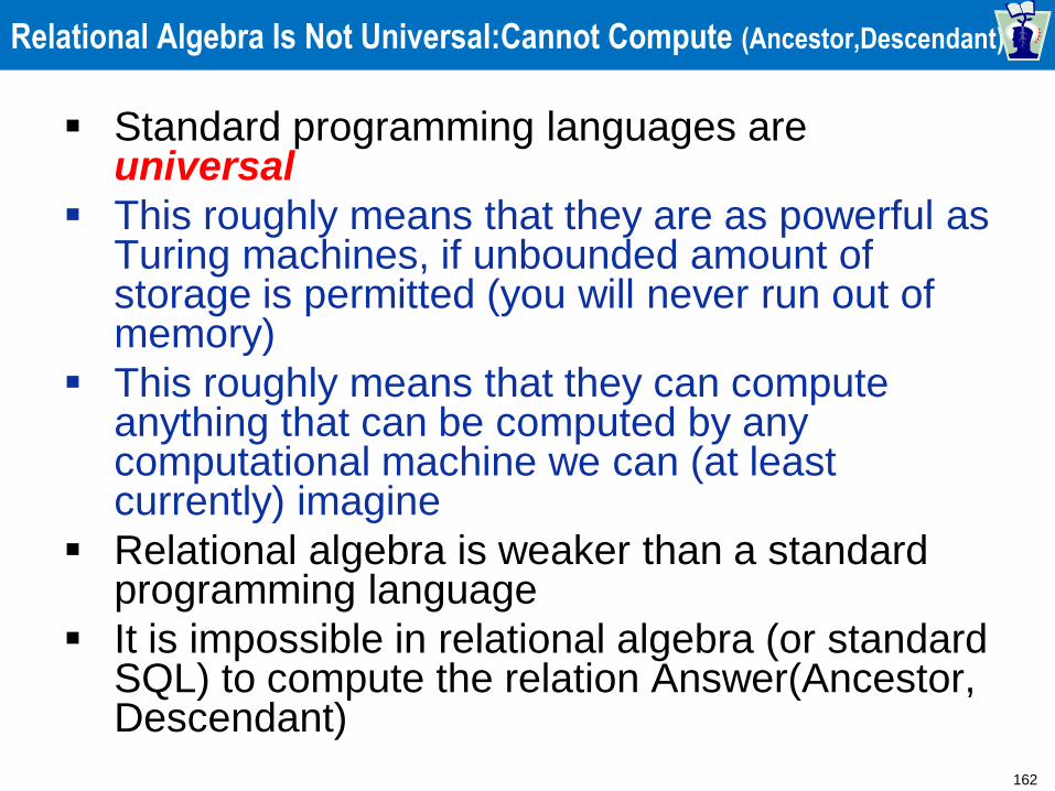
Standard programming languages are universal
This roughly means that they are as powerful as Turing machines, if unbounded amount of storage is permitted (you will never run out of memory)
This roughly means that they can compute anything that can be computed by any computational machine we can (at least currently) imagine
Relational algebra is weaker than a standard programming language
It is impossible in relational algebra (or standard SQL) to compute the relation Answer(Ancestor, Descendant)
163
Relational Algebra Is Not Universal: Cannot Compute (Ancestor,Descendant)
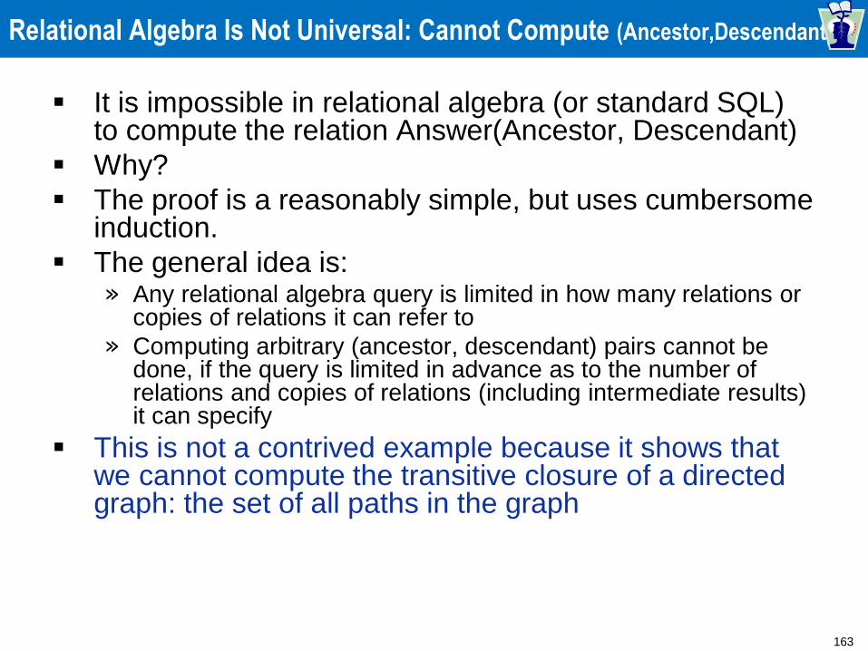
It is impossible in relational algebra (or standard SQL) to compute the relation Answer(Ancestor, Descendant)
Why?
The proof is a reasonably simple, but uses cumbersome induction.
The general idea is: » Any relational algebra query is limited in how many relations or
copies of relations it can refer to
» Computing arbitrary (ancestor, descendant) pairs cannot be done, if the query is limited in advance as to the number of relations and copies of relations (including intermediate results) it can specify
This is not a contrived example because it shows that we cannot compute the transitive closure of a directed graph: the set of all paths in the graph
164
A Sample Query
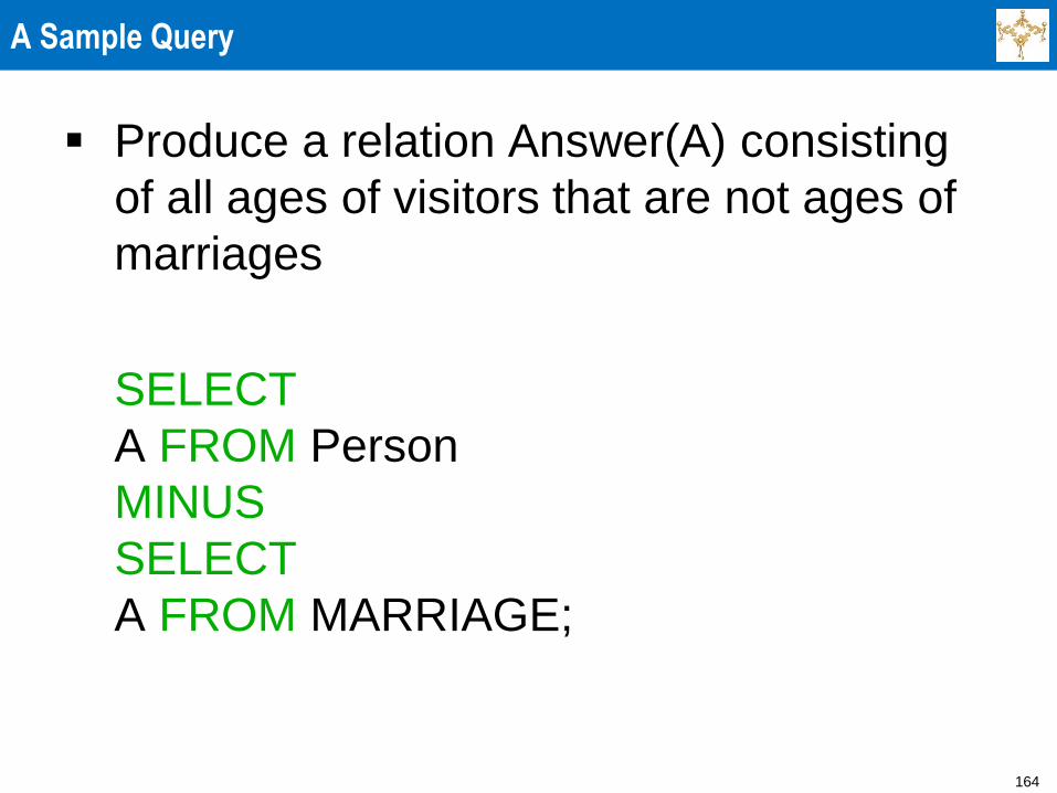
Produce a relation Answer(A) consisting
of all ages of visitors that are not ages of
marriages
SELECT
A FROM Person
MINUS
SELECT
A FROM MARRIAGE;

165
The Query In Microsoft Access
We do not show this here, as it is done in
a roundabout way and we will do it later
166
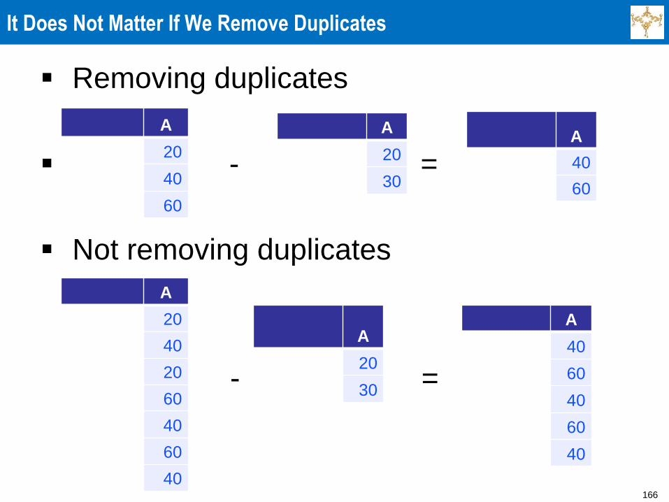
It Does Not Matter If We Remove Duplicates
Removing duplicates
- =
Not removing duplicates
- =
A
20
40
20
60
40
60
40
A
20
30
A
40
60
40
60
40
A
20
40
60
A
20
30
A
40
60
167
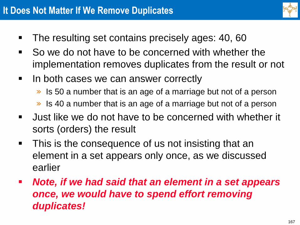
It Does Not Matter If We Remove Duplicates
The resulting set contains precisely ages: 40, 60
So we do not have to be concerned with whether the
implementation removes duplicates from the result or not
In both cases we can answer correctly
» Is 50 a number that is an age of a marriage but not of a person
» Is 40 a number that is an age of a marriage but not of a person
Just like we do not have to be concerned with whether it
sorts (orders) the result
This is the consequence of us not insisting that an
element in a set appears only once, as we discussed
earlier
Note, if we had said that an element in a set appears
once, we would have to spend effort removing
duplicates!
168
Now To “Pure” Relational Algebra
This was described in several slides
But it is really the same as before, just the
notation is more mathematical
Looks like mathematical expressions, not
snippets of programs
It is useful to know this because many
articles use this instead of SQL
This notation came first, before SQL was
invented, and when relational databases
were just a theoretical construct
169
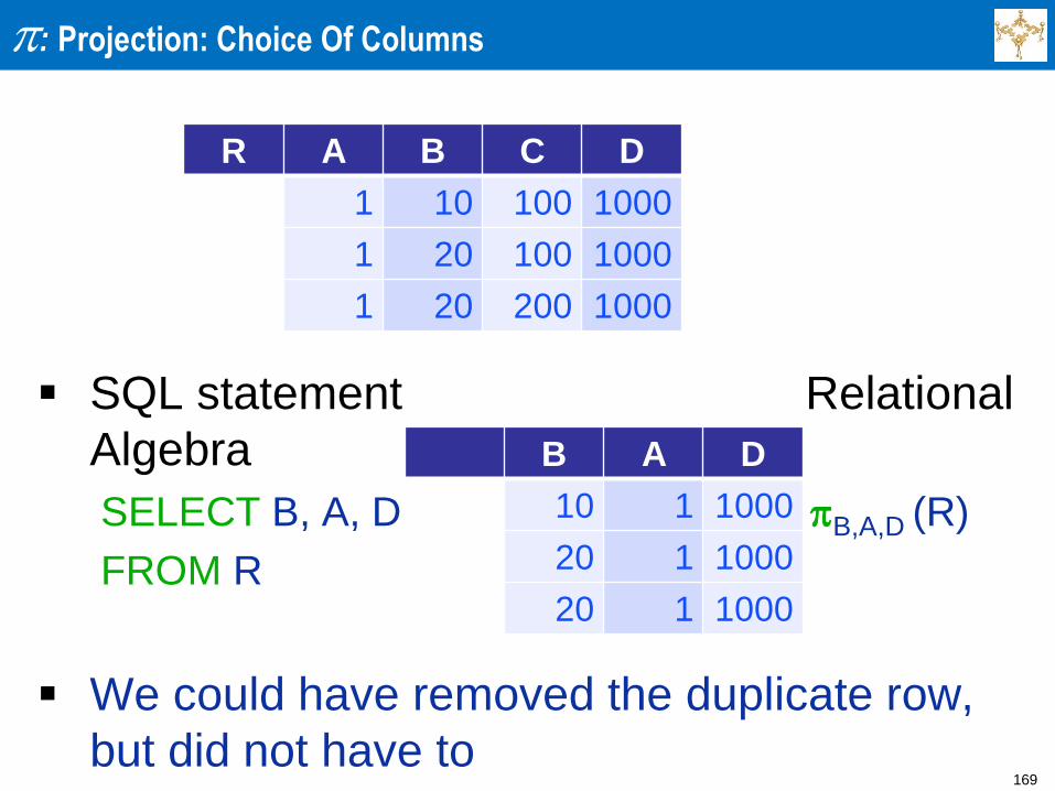
: Projection: Choice Of Columns
SQL statement Relational
Algebra
SELECT B, A, D B,A,D (R)
FROM R
We could have removed the duplicate row,
but did not have to
R A B C D
1 10 100 1000
1 20 100 1000
1 20 200 1000
B A D
10 1 1000
20 1 1000
20 1 1000
170
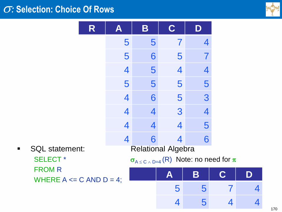
: Selection: Choice Of Rows
SQL statement: Relational Algebra
SELECT * A C D=4 (R) Note: no need for
FROM R
WHERE A <= C AND D = 4;
R A B C D
5 5 7 4
5 6 5 7
4 5 4 4
5 5 5 5
4 6 5 3
4 4 3 4
4 4 4 5
4 6 4 6
A B C D
5 5 7 4
4 5 4 4
171
Selection
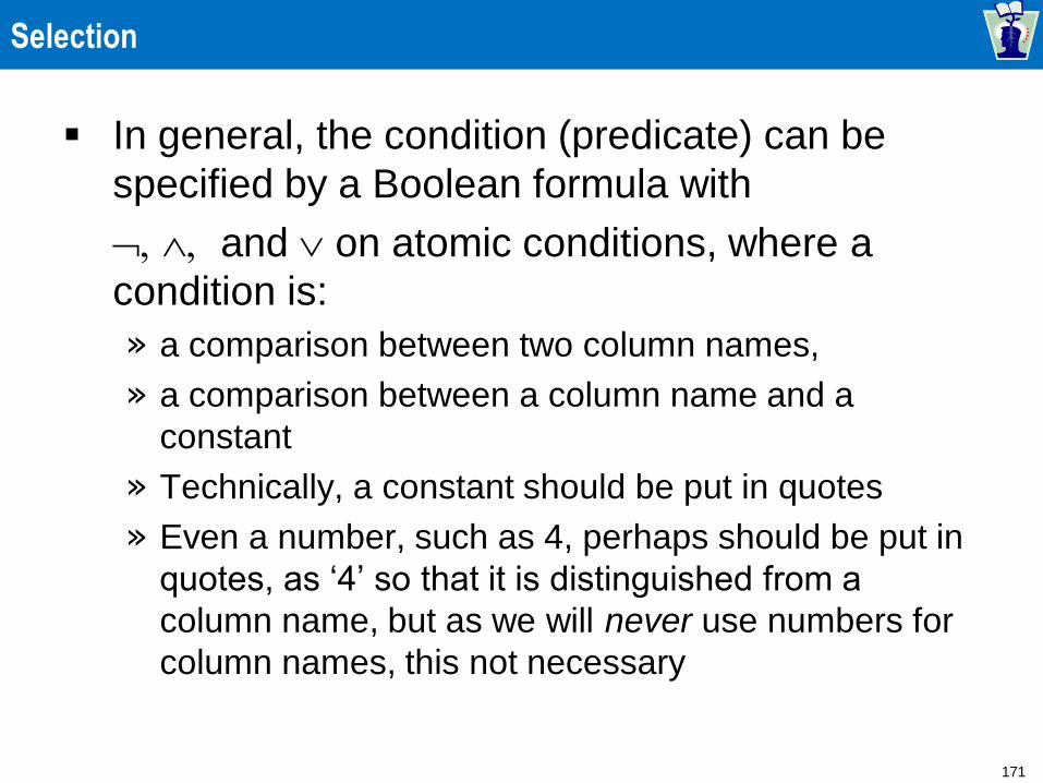
In general, the condition (predicate) can be
specified by a Boolean formula with
and on atomic conditions, where a
condition is:
» a comparison between two column names,
» a comparison between a column name and a
constant
» Technically, a constant should be put in quotes
» Even a number, such as 4, perhaps should be put in
quotes, as ‘4’ so that it is distinguished from a
column name, but as we will never use numbers for
column names, this not necessary
172
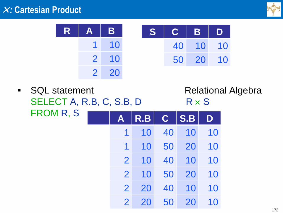
: Cartesian Product
SQL statement Relational Algebra
SELECT A, R.B, C, S.B, D R S
FROM R, S
A R.B C S.B D
1 10 40 10 10
1 10 50 20 10
2 10 40 10 10
2 10 50 20 10
2 20 40 10 10
2 20 50 20 10
R A B
1 10
2 10
2 20
S C B D
40 10 10
50 20 10
173
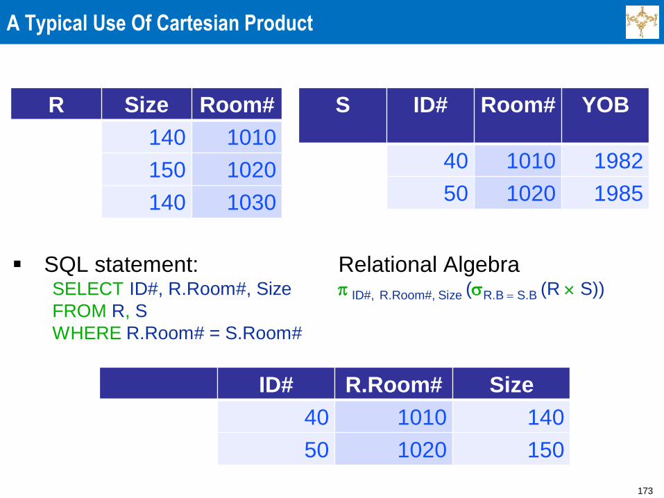
A Typical Use Of Cartesian Product
SQL statement: Relational Algebra SELECT ID#, R.Room#, Size ID#, R.Room#, Size (R.B = S.B (R S))
FROM R, S
WHERE R.Room# = S.Room#
R Size Room#
140 1010
150 1020
140 1030
S ID# Room# YOB
40 1010 1982
50 1020 1985
ID# R.Room# Size
40 1010 140
50 1020 150
174
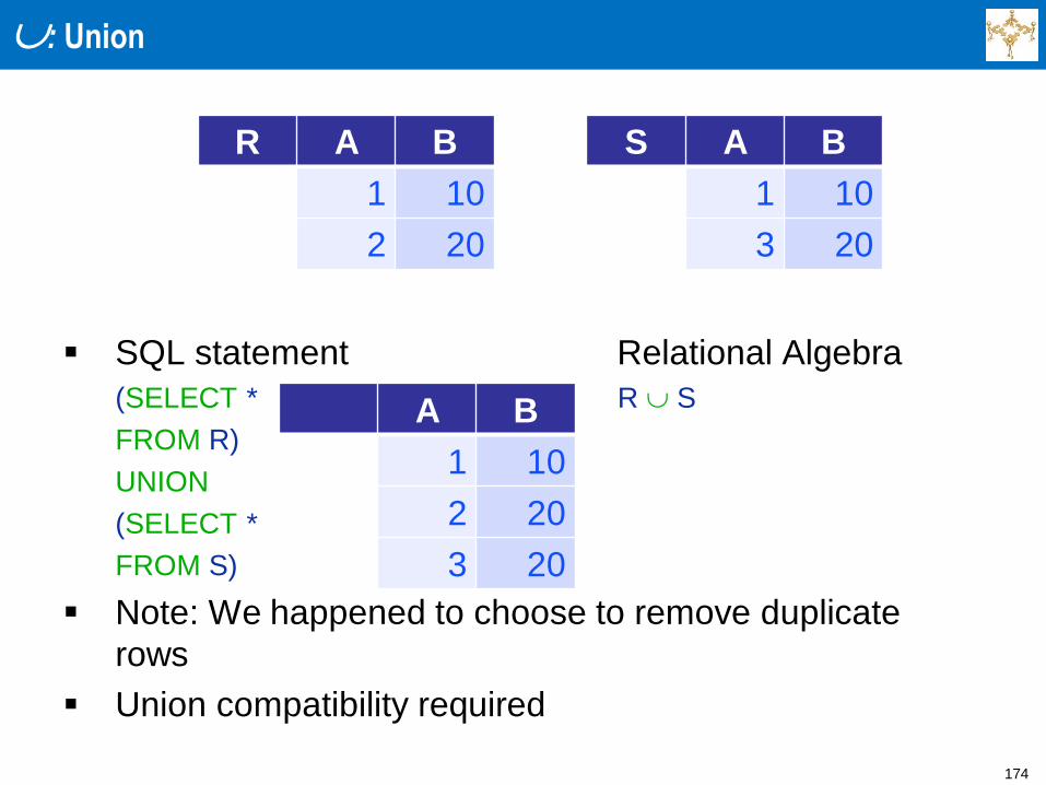
: Union
SQL statement Relational Algebra
(SELECT * R S
FROM R)
UNION
(SELECT *
FROM S)
Note: We happened to choose to remove duplicate
rows
Union compatibility required
R A B
1 10
2 20
S A B
1 10
3 20
A B
1 10
2 20
3 20
175
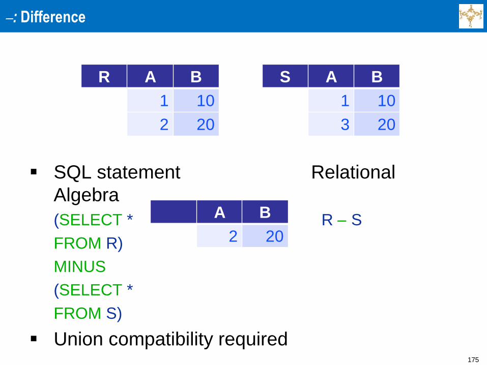
-: Difference
SQL statement Relational
Algebra
(SELECT * R - S
FROM R)
MINUS
(SELECT *
FROM S)
Union compatibility required
R A B
1 10
2 20
S A B
1 10
3 20
A B
2 20
176
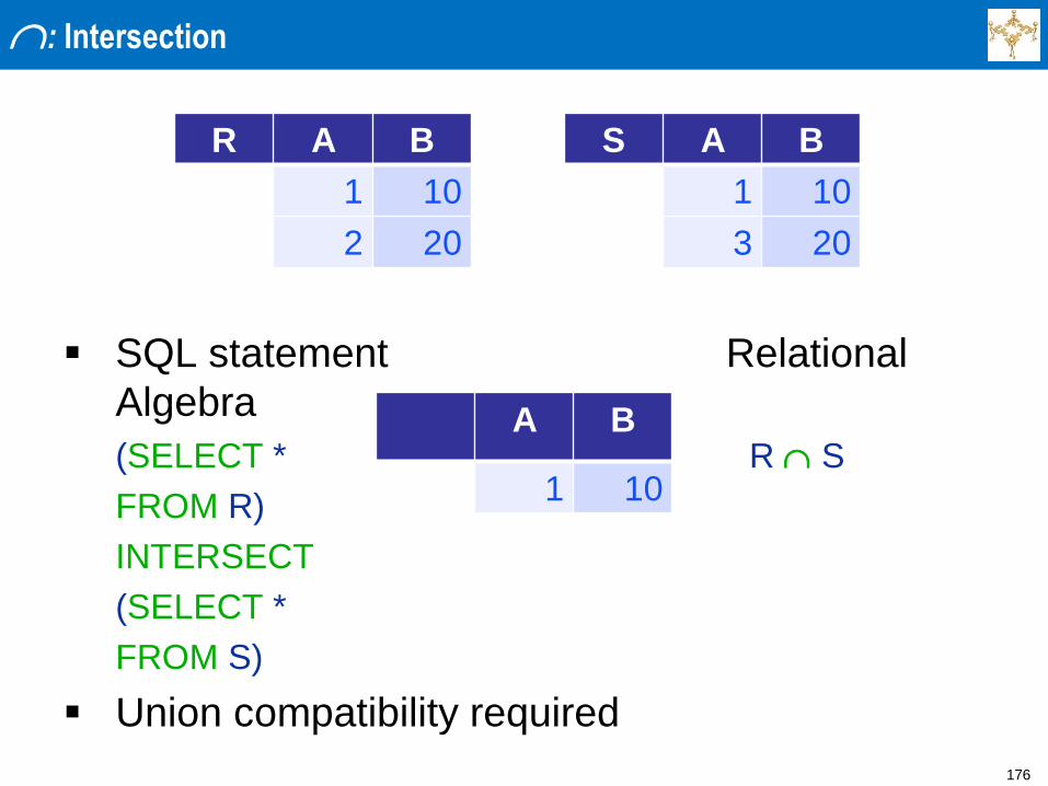
: Intersection
SQL statement Relational
Algebra
(SELECT * R S
FROM R)
INTERSECT
(SELECT *
FROM S)
Union compatibility required
R A B
1 10
2 20
S A B
1 10
3 20
A B
1 10
177
Summary (1/2)
A relation is a set of rows in a table with labeled columns
Relational algebra as the basis for SQL
Basic operations:
» Union (requires union compatibility)
» Difference (requires union compatibility)
» Intersection (requires union compatibility); technically not a basic
operation
» Selection of rows
» Selection of columns
» Cartesian product
These operations define an algebra: given an expression
on relations, the result is a relation (this is a “closed”
system)
Combining this operations allows production of
sophisticated queries
178
Summary (2/2)
Relational algebra is not universal: We can write
programs producing queries that cannot be
specified using relational algebra
We focused on relational algebra specified
using SQL syntax, as this is more important in
practice
The other, “more mathematical” notation came
first and is used in research and other venues,
but not commercially
179
Agenda
1 Session Overview
4 Summary and Conclusion
2 Relational Algebra and Relational Calculus
3 Relational Algebra Using SQL Syntax
180
Summary
Relational algebra and relational calculus are formal
languages for the relational model of data
A relation is a set of rows in a table with labeled columns
Relational algebra and associated operations are the
basis for SQL
These relational operations define an algebra
Relational algebra is not universal as it is possible to write
programs producing queries that cannot be specified
using relational algebra
Relational algebra can be specified using SQL syntax
The other, “more mathematical” notation came first and is
used in research and other venues, but not commercially
181
Assignments & Readings
Readings
» Slides and Handouts posted on the course web site
» Textbook: Chapters 6, 8
Assignment #5
» Textbook exercises: Textbook exercises: 8.15, 8.18, 8.22, 8.30, 6.8, 6.12
Project Framework Setup (ongoing)
182
Next Session: Standard Query Language (SQL) Features
SQL as implemented in commercial
databases

183
Any Questions?