1

Productivity Spillovers from Foreign Direct Investment:

Evidence from Firm-Level Data in China

Xinpeng Xu* and Yu Sheng **

Abstract Using firm-level census data, this paper examines the spillover effects of foreign direct investment (FDI) on domestic firms in the Chinese manufacturing industry between 2000 and 2003. We find that FDI has a significant positive spillover on industry productivity that decreases as the share of FDI in the industry increases. These positive spillovers are more likely to occur through forward linkage (where domestic firms purchase high-quality intermediate goods or equipment from foreign suppliers) than through backward linkage (where firms produce goods for foreign multinationals). Entering and exiting firms receive greater benefits from both horizontal and vertical productivity spillovers than existing firms. Benefits are also highest in large, non-exporting and non-SOE firms. Our evidence suggests that domestic firms differ significantly in the extent to which they benefit from FDI according to firm structure as well as the source of FDI. Keywords: Foreign Direct Investment, Spillover Effects, Chinese Manufacturing Industry JEL Code: F21; F23 * Xinpeng Xu (Corresponding author) Faculty of Business Hong Kong Polytechnic University Kowloon, Hong Kong afxxu@polyu.edu.hk ** Yu Sheng Crawford School of Economics and Government The Australian National University Canberra, Australia yu.sheng@anu.edu.au

2

I. Introduction

Over the past two decades, cross-border flows of foreign direct investment (FDI) have taken

centre stage in the globalization process, with increasing numbers of firms (usually developed

countries) investing in foreign countries (either developed or developing countries). According to

UNCTAD (2007), the global flows of FDI increased from US$324 billion in 1995 to US$1.3

trillion in 2006. Inflows of FDI to developed countries amounted to US$857 billion in 2006

while rising to a record US$379 billion for developing countries. The global stock of FDI has

thus more than quadrupled from US$2.76 trillion in 1995 to $12 trillion in 2006.

A commonly-held belief is that FDI benefits recipient countries through knowledge transfer from

multinational firms, which helps improve the productivity of domestic firms. There are several

channels through which FDI may affect domestic productivity. First, domestic firms may benefit

by observing and imitating the multinationals (horizontal spillovers). Second, productivity

spillovers may occur because of labor turnover, as former employees of multinationals, who

have acquired managerial expertise, production or marketing skills, may resurface in domestic

firms or set up their own firms to which they can transfer that knowledge (horizontal spillovers).

Third, domestic firms may also benefit through backward linkage, by being a supplier of the

multinationals and thereby obtaining some free technology transfer, or through forward linkage

by having a foreign supplier (vertical spillovers).

Despite these perceived relationships, empirical evidence of the benefits of FDI spillovers is

sobering (Rodrik 1999). Due to a lack of detailed firm-level data, researchers have focused

mainly on developed countries such as the U.S. (Haskel et al., 2007) and UK (Griffith et al.,

2006), which as technological leaders may have little to gain from FDI spillovers. Other studies

focus on small developing countries where the amount of FDI is relatively small and domestic

industries are not sufficiently diversified to reap significant benefits from FDI. For example,

Aitken and Harrison (1999) estimate the productivity effects of FDI to a sample of Venezuelan

manufacturing plants from 1976 to 1989, and find that plants in industries with a higher foreign

presence actually had lower productivity than those in other industries. Javorick (2004) finds that

domestic firms in Lithuania only benefit from FDI when they are the suppliers to foreign firms.

3

Recently, Blalock and Gertler (2007) found positive horizontal spillover effects of FDI in

Indonesian manufacturing, but argue that lower input prices due to the presence of downstream

FDI are a major source of the heightened domestic productivity.

What is lacking in the literature is firm-level evidence from a large FDI recipient country in the

developing world where any spillover effects may be most important. This paper fills the gap by

examining the case of China. Using annual manufacturing census data of firms (including all

state-owned enterprises and non-stated firms with annual sales of more than RMB 5 million

(about US$600,000)) for the years 2000 to 2003, we study the effects of FDI on domestic-firm

productivity in the manufacturing sector. Such a study is of interest for several reasons. First,

China is the largest recipient of FDI in the developing world, recording US$69 billion of inflows

and a total FDI stock of US$292 billion in 2006. This level of FDI appears sufficiently large for

China to reap horizontal benefits. Second, China’s history under centralised planning led to

unique industry development. As the economy has opened to foreign direct investment, this wide

spectrum of industries has a high potential to benefit from backward and forward linkages with

foreign firms. Third, as a developing economy, China’s distance from the technology-and-

management frontier may place it in an ideal position to exploit the potential benefits of FDI

(Findlay 1978), relative to more advanced industrialized nations.

We contribute to the literature in several ways. By using census data we are able to undertake a

full-scale examination of firm-level FDI spillover in China.1 Further, our empirical analysis

overcomes with a variety of problems typically associated with this type of analysis; including

endogeneity of input choices, omitted variables and clustering effects in standard errors. In

particular, we differ from other publications by controlling for clustering effects. As well as

identifying the spillover effects on existing firms as commonly undertaken, we extend our

analysis to identify the productivity effects of foreign investment on entering and exiting firms.

Finally, we explore the role of heterogeneity in firms and in FDI sources and investigate whether

certain firm characteristics (such as ownership structure and export orientation) have

implications for FDI benefits.

1 There are some studies on the spillover effect of FDI in China using industry-level data (e.g.,Sun et al.,2002). Industry-level studies, however, suffer from problems such as aggregation bias and endogeneity, as discussed in Hale and Long (2007) and Haskel et al. (2007, Footnote 2). Hu and Jefferson (2002) study FDI spillovers in China’s electronic and textile industries.

4

Our results indicate that there are significant positive horizontal spillovers from FDI. Chinese

domestic firms in an industry with high FDI can produce a greater output (for a given level of

inputs) than otherwise similar firms in industries with low FDI. The result is in stark contrast

with most empirical studies on small developing countries that find negative or no spillovers

(Aitken and Harrison 1999, among others). However, positive effects diminish as the share of

FDI in an industry increases, and become negative when the share of FDI in that industry reaches

a certain threshold. Our results capture both positive spillovers and negative “business stealing”

effects: when FDI is below a certain level, domestic firms may benefit more from its presence

just by observing and imitating the multinationals and perhaps through labor turnover; yet when

FDI increases to a certain level, “business stealing” effects dominate.

Furthermore, the positive spillovers are more likely to operate through forward linkage when

domestic firms purchase high-quality intermediate goods with lower input prices, or equipment

from foreign suppliers, than through backward linkage when they produce for multinationals as

commonly found in other (small) developing countries. This may be the result of a set of unique

Chinese FDI policy that encourages firms to import raw materials and equipments from

international market.

The magnitude of the horizontal and forward linkage effects is economically meaningful. A one

percentage point increase in the share of foreign firms in an industry leads to a 0.015 percent

productivity gain for domestic firms in the same industry and a 0.057 percent productivity gain

for domestic firms in the downstream industry. Most important, we find that newly entering and

exiting firms benefit more from foreign investment than incumbent firms. We find that estimated

elasticities of both horizontal and forward linkage effects of FDI on all domestic firms are 0.029

and 0.070 respectively, which are much higher than the effects on continuing firms (domestic

firms excluding new entry and exit) where the elasticities are 0.009 and 0.051 respectively. We

also find that domestic firms differ significantly in the extent to which they benefit from FDI,

with large, non-exporting and non-SOE firms accruing the greatest benefits from foreign firms in

China.

5

Not only is there significant heterogeneity across firms in absorbing the benefits of FDI

spillovers, but also sources of FDI matter for the spillovers, with FDI coming from Western

firms produce more substantive spillovers than overseas Chinese firms. This is consistent with

observations that the Hong Kong and Taiwan firms investing in China are usually less capital-

intensive and technologically advanced than their Western counterparts. Also, these firms are

often “round-trip” firms taking advantage of China’s preferential tax treatment for foreign

investors.

The rest of the paper is organized as follows. The next section describes in detail the background

of FDI in China. Section III discusses the construction of our dataset and provides basic statistics,

as well as the parameter-identification strategy implemented. Section IV discusses the results.

Section V concludes.

II. Overview of Foreign Direct Investment in China

Although China’s first experience with FDI came after the reforms of 1978, it was not until 1992

that high levels of FDI started to flow into the country. Figure 1 reports the utilized inflow during

the period of 1992 to 2006. Between 1992 and 2006, FDI inflows increased from US$1.1 billion

to $73 billion. In particular, after its entry into the WTO in 2001, China’s commitment to broader

and deeper liberalization in trade and investment further accelerated FDI inflows and increased

the share of foreign ownership in Chinese assets. In 2006, the share of FDI inflow in total fixed-

asset investment reached 5.28 percent, with the manufacturing sector the largest recipient of FDI

in China, accounting for 63.6 percent of the total FDI.2

China’s policy objectives in attracting FDI are to advance China’s technology and to promote

exports, articulated in Article 3 of the Law of the People's Republic of China on Foreign-owned

Enterprises: “…[China] encourage the establishment of foreign-owned enterprises that are

export-oriented or technologically advanced.” To promote exports to China from foreign firms,

China offers import tariff and value-added tax (VAT) exemption for imported raw materials and

2 Source: http://www.fdi.gov.cn.

6

parts used in the export processing. This tax incentive encourages foreign firms to purchase

inputs from, and to export their output to, the international market. In fact, imports by foreign

firms accounted for almost 59 percent of China’s total imports while exports by foreign firms

accounted for 57 percent of China’s total exports in 2007.3 Consequently, most foreign firms in

China are exported-oriented. An unintended consequence of the tax incentive has been a

weakening vertical linkage between foreign firms and local Chinese firms, in particular, a lack of

backward linkage with those Chinese firms in the upstream industry.4

China also offers various preferential treatments to foreign firms if their investment falls into the

so-called ‘high-tech’ sector. Within the manufacturing sector, FDI has started to move from

labor-intensive industries, where FDI was initially concentrated, to capital-intensive and

technology-intensive industries. From 2001 to 2005, the growth in total assets of foreign firms

was greatest in the most technology-intensive industries — increasing by 137 percent —

followed closely by capital-intensive industries, which increased by 125 percent, though foreign

firms’ total assets in labor-intensive industries increasing by 81 percent.5 The inflow of FDI with

relatively advanced technology into Chinese manufacturing offered ample opportunities for

domestic firms to improve their productivity.

FDI inflows into China contribute significantly to the process of marketization in the

manufacturing sector. In 2006, the total output value of FDI firms add up to 6.09 trillion RMB,

accounting for 47.5 percent of the total output value of private enterprises in Chinese

manufacturing sector. With more foreign firms entering into Chinese manufacturing sector, state

owned enterprises (SOEs) are less dominant. Due to the intensified market competition, more

productive firms enter while less efficient firms exit freely. Between 2000 and 2003, the average

Herfindahl concentration index, defined as the output share of top eight firms across 21 two-digit

level manufacturing industries decreased from 8.7 per cent to 8.5 per cent as the average FDI

output share increased from 29.0 per cent to 30.5 per cent.

3 See http://www.fdi.gov.cn. 4 China also allows imported inputs sold to downstream firms to be exempt from import tariff and VAT tax as long as they are processed for export. 5 The nine sectors with the most significant expansion of foreign firms are furniture (183 percent), chemical materials and products (128 percent), ferrous metal smelting (297 percent), non-ferrous metal smelting (193 percent), general machinery (145 percent), special machinery (206 percent), transport equipment (134 percent), electronics and telecommunications equipment (146 percent), and instruments (169 percent), most of which are capital-intensive and technology-intensive industries (reference?).

7

A distinct feature of FDI in China has been the sources of investment. The bulk of FDI in China

is from newly-industrialized Asian economies with similar culture and traditions rather than from

Westernized economies. In particular, FDI from Hong Kong and Taiwan (HKTW) accounts for

around half of the total FDI inflow to mainland China while less than one third is from

developed economies. There are mixed views in the literature as to how HKTW firms provide

benefit to local firms. Although investors of Chinese ethnicity have the added advantage of

cultural and language similarities, their technology is typically regarded as less advanced. The

variability in productivity spillovers from FDI in China, based on the investment source, remains

an empirical question.

III. Data and Estimation Strategy

A. Data Collection and Variable Definition

The data used in this study is derived from from the Annual Enterprise Census conducted by the

National Bureau of Statistics (NBS) of China. The census covers all state-owned firms and non-

state-owned enterprises with annual sales above RMB ¥5 million in mining, manufacturing and

public-utility sectors, across all provinces. These sectors account for more than 95 percent of the

total value of Chinese industrial output. The sample used is an unbalanced dataset at the firm

level for the manufacturing sector (China Industry Classification Code: 13-42), which spans the

four year period from 2000 to 2003. The number of firms sampled varies from 134,130 in 2000

to 169, 810 in 2003.

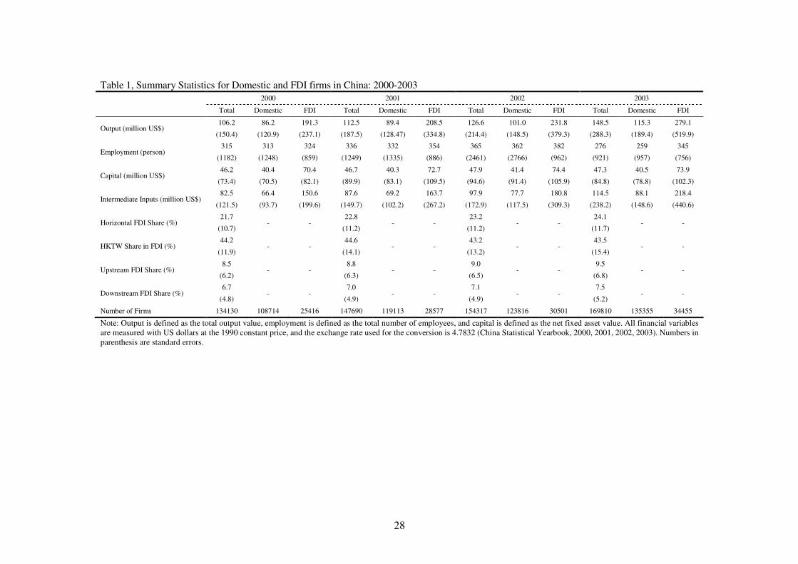
Table 1 provides summary data for the period including the number of firms, the value of their

average output, their average use of labor and capital, and the intermediate inputs of domestic

firms and FDI firms. The real output of firms, Y, is defined as the total value of the sample firms’

outputs, deflated by the producer price index at the firm level, with 1990 as the base year.6

Labor input, L, is defined as total employment. As employment data are not available for 2003,

we use registered labor (“Zai Gang”) as a substitute. Although there are large numbers of non-

6 Some studies have used industry-specific price index to deflate firm output, which may not be appropriate as it imposes a strong assumption that all firms faced the same prices (see Klette and Griliches (1996) for a discussion).

8

productive workers in Chinese firms, there is strong correlation (about 95 percent) between total

employment and “Zai Gang” labor at the firm level in 2000. Therefore, we use “Zai Gang”

workers as a proxy for total employment in 2003 given data availability. Capital, K, is defined as

the value of fixed assets at the end of the year, deflated by the price index for investment goods,

with 1990 as the base year. As defined by the Chinese National Bureau of Statistics, intermediate

goods, M, is the value of total output less value added, plus the net value-added tax, deflated by

the intermediate-input deflator.

Following Javorick (2004), we measure FDI in an industry by calculating the weighted sum of

foreign capital, with the weight being each firm’s share of industry output ( jtFDIShare ):

)/()*( ∑∑∈∈

=ji

it

ji

ititjt YYreForeignShaFDIShare , (1)

where i denotes firm, j denotes industry and t year. The index is calculated at the two-digit

level.7

Table 1 also shows the average share of foreign equity during the period 2000-2003, measured as

capital share of FDI by output. There is a significant increase over time in the shares of foreign

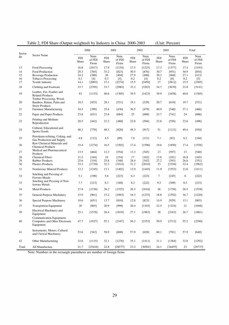
equity. Table 2 shows the distribution of FDI firms and their shares (output-weighted) across

industries at the two-digit level within the manufacturing sector during the sample period. The

industry that had the largest shares of foreign investment is “Instruments, Meters, Cultural and

Clerical Machinery” (57.9%), followed by “Communication Equipment, Computers and Other

Electronic Equipment” (55.2%), “Cultural, Educational and Sports Goods” (49.4%) and “Leather,

Fur, Feather and Related Products” (40.6%).

Finally, we use jtHKTWRatio as an index to distinguish the spillover effects of foreign capital

from Hong Kong and Taiwan from other sources, where:

7 See Aitken and Harrison (1999) and Javorcik (2004) for the output-penetration index. To test for robustness, we also provide an alternative measure of FDI in a sector by calculating the weighted sum of foreign capital, with the weight being each firm’s share

of capital in the sector (itKFDI ).

9

)*_/()*_( ∑∑∈∈

=ji

ititit

ji

itjt YOtherreForeignShaYHKTWreForeignShaHKTWRatio (2)

where itHKTWreForeignSha _ and itOtherreForeignSha _ are the weighted sum of capital from

Hong Kong SAR and Taiwan and other foreign countries respectively.

The backward and forward linkages of FDI, jtBackwardFDI _ and jtForwardFDI _ , are

defined, following Javorick (2004), as follows:

∑≠

=jk

ktjkjt FDIShareBackwardFDI α_ (1A)

and

∑ ∑∑≠ ∈∈

−−=jm mi

itit

mi

itititjmjt XYXYreForeignShaForwardFDI ])](/[)](*[[_ ϕ , (1B)

where jkα is the proportion of industry j’s output supplied to industry k, derived from the 1997

input-output table at the two-digit International Standard Industrial Classification (ISIC) level,

and jmϕ is the share of inputs purchased by industry j from industry m in total inputs sourced by

industry j. itY is the total output and

itX is the export of firm i at time t

B. Specification and Identification

To examine whether FDI generates intra-industry or inter-industry productivity spillovers to

domestic firms, we start with a specification that has been used extensively in the literature; e.g.,

Aitken and Harrison (1999) and Javorcik (2004):

ijrttrj

jtjt

jtjtjt

ijrtijrtijrtijrtijrt

ForwardFDIBackwardFDI

HKTWRatioFDIShareFDIShare

fdiMKLY

εααα

ββ

βββ

γββββ

++++

++

+++

++++=

__

lnlnln

87

6

2

54

3210

(3)

where ijrtY denotes the real output of domestic firm i operating in industry j and region r at

time t , ijrtL , ijrtK and ijrtM are labor, capital and intermediate production inputs, respectively,

ijrtfdi is the capital share of foreign investment in domestic firms at the firm level. jtFDIShare

10

and its square term measure the share of foreign equity in industry j at time t ,8 which takes the

form of jtYFDI and its square term. jtBackwardFDI _ and jtForwardFDI _ are defined as the

backward and forward linkages of FDI, jtHKTWRatio represents the relative share of foreign

equity owned by investors from Hong Kong and Taiwan. Three sets of dummy variables are used

to control for the industry-, region- and time-specific effects, respectively. They include

∑=j

jjj dϖα for the industry-specific effect, ∑=r

rrr dχα for the region-specific effect, and

∑=t

ttt dδα for the time-specific effect.

To correctly identify the effects of FDI on domestic productivity, we need to address several

econometric issues such as endogeneity of input choices, cluster effects and omitted variables

Endogeneity of Input Choices — Ordinary least squares (OLS) is inappropriate for estimating

the impacts of labor and capital on productivity, since factors of production should be treated as

endogenous. Olley and Pakes (1996) (OP), followed by Levinsohn and Petrin (2003) (LP), point

out that inputs like capital should be considered endogenous since producers chooses the level or

usage rate based on cost and productivity considerations. These considerations are observed by

the producer but not by the econometrician. Thus, productivity estimates may be biased if the

endogeneity of input choice is not taken into account.

To address this concern, we employ a semi-parametric estimation procedure suggested by

Levinsohn and Petrin (2003). Compared with the approach of Olley and Pakes (1996), this

approach allows for firm-specific productivity differences that exhibit idiosyncratic changes over

time, and use intermediate inputs rather than long-term capital investment as a proxy for

unobserved productivity. We follow the LP method for two reasons. Firstly, investment behavior

in Chinese firms is highly influenced by government policy (such as policy loans to SOEs) so

investment may not be monotonic with respect to productivity. Secondly, the four year data

sample available is not sufficiently long for firms to make capital adjustments, especially in

regard to long-term investments such as buildings and machinery. More specifically, we assume

8 An alternative measure would use each firm’s share in the aggregate industrial capital.

11

a Cobb-Douglas production function, written as a natural-logarithm after taking the first order

differentiation:

itititmitkitlcit umkly +++++= ϖββββ (4)

where cβ measures the mean efficiency level across firms and over time,

itϖ represents firm-

level productivity, and itu is an i.i.d. component, representing unexpected deviations from the

mean due to measurement error, unexpected delays or other external circumstances. The three

components combine to determine the time-specific and producer-specific outputs.

In order to estimate Equation (4), we further assume that capital is a state variable only affected

by current and past levels of unobserved productivity ( itϖ ) and monotonic with respect to the

intermediate inputs. We define

),( itittit kgm ϖ= ( Tt ,...,1= ) (5)

where itm is a vector of proxy variables (i.e. intermediate inputs) and g(·,·) is monotonic with

respect to itϖ . The choice of intermediate inputs hence depends on capital and productivity.

Provided that the choice of intermediate inputs is strictly increasing, conditional on capital, the

relationship between itm and

itϖ can be inverted. Thus, we have ),( itittit mkh=ϖ where

(.,.)(.,.) 1−= tt gh . Substituting this information into Equation (4), we have

ititittitmitkitlit umkhmkly +++++= ),(0 ββββ (6)

Estimation of Equation (6) is carried out in two stages. In the first stage, we define

),(),( 0 itittitmitkitit kmhmkkm +++= βββφ (in LP). Thus, OLS method can be used to estimate

ititititlit ukmly ++= ),(φβ (7)

12

where (.,.)φ is approximated by a higher-order polynomial in itm and

itk (including a constant

term). Estimation of Equation (7) results in a consistent estimate of the coefficients for labor. In

the second stage, assume that productivity follows a first-order Markov process, i.e.

111 )|( +++ += itititit E ξϖϖϖ , where 1+itξ , representing the news component, is assumed to be

uncorrelated with productivity and capital in period 1+t . Thus, the estimation algorithm can be

written as:

1111011 )|(][ ++++++ ++++=− itititititkitlit uEklyE ξϖϖβββ (8)

where )()|( 1 itmitkititit mkqE ββφϖϖ −−=+ follows from the law of motion for the productivity

shock. As the first stage of the estimation procedure has used a higher-order polynomial

expansion in itkit kβφ ˆˆ − or

itmitkit mk ββφ ˆˆˆ −− to approximate g(·,·), the capital coefficients can

then be obtained by applying Non-Linear Least Squares (NLS) to Equation (9):

1111011 )( ++++++ ++−−+++=− itititmitkititmitkitlit umkqmkly ξββφββββ . (9)

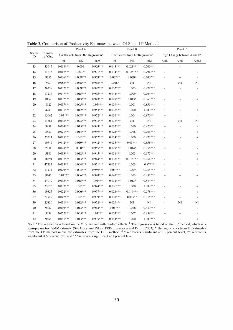
By using this method, we can obtain accurate production-function estimates that can in turn be

used to estimate domestic productivity; or ijrtmijrtkijrtlijrtijrt mklyTFP lnlnlnln βββ −−−= .

Both the OLS and our estimates are shown in Table 3. Using the productivity estimate as the

dependent variable, we obtain from equation (3):

ijrttrj

jtjtjt

jtjtijrtijrt

ForwardFDIBackwardFDIHKTWRatio

FDIShareFDISharefdiTFP

εααα

βββ

ββγβ

++++

+++

+++=

__

ln

876

2

540

. (10)

Cluster Effect — The OLS estimates may overestimate the spillover effects of FDI on domestic

firm productivity without a correction for clustering. Moulton (1990; p.334), followed by

Bertrand et al. (2004), argues that “when one tends to use the aggregate market or public policy

13

variables to explain the economic behavior of micro units, it is possible that the standard errors

of estimated coefficients of those aggregate variables from OLS might be underestimated, which

would lead to the overstated significance of coefficients.” The presence of group-level variables

in such a ‘structural’ model can be viewed as putting additional restrictions on the intercepts in

separate-group models, which can cause the residual to deviate from the i.i.d assumption. Failure

to address this type of cluster error problem may cause a serious downward bias in the estimated

errors, resulting in spurious findings of statistical significance for the aggregate variable of

interest (industry FDI in this case).

Javorcik (2004) uses a simple cluster-robust option to correct for any intra-group correlation in

standard errors between observations belonging to the same industry in a given year. Although

this represents an improvement over previous studies that do not correct for cluster effects, the

method of allowing for differences in the variance/standard errors due to arbitrary intra-group

correlation has limitations (Wooldridge, 2006). To illustrate the potential risk that the simple

cluster-robust correction can bring about, we suppose there is a cluster effect in equation (10).

Then, the residual part can be decomposed into two components: ir

g

jtijrt vu +=ε . Thus, the

variance of the residual in the regression could be written as:

gvuijrt M/: 22 σσσε ε += (11)

where ijrtε is the residual of Equation (10), εσ is the variance of

ijrtε . 2

uσ is the variance of the

inter-group residual ( g

jtu ), 2

vσ is the variance of the intra-group residual (irv ), and

gM is the

number of observations in each group. In such a situation, the cluster-robust option will work

only when g

jtu is normally distributed with constant variance and when it dominates ijrtε so that

either 2

vσ is small relative to 2

uσ , gM is large, or both. In many FDI studies, however, the

number of groups (say, two-digit industries in a single time period) is small (M<<50) (i.e., 2

vσ is

small relative to 2

uσ ) and there are very unbalanced cluster sizes in the sample (some gM may be

14

small) so that εσ may not be constant and dominated by 2

uσ .9 Therefore, the cure provided by

the cluster-robust correction can be even worse than the disease, since using the wrong weights

may bias the standard errors of the estimated coefficients in an unclear direction.10

To properly correct for cluster effects in standard errors of the estimated coefficients, we follow

a new two-stage estimation procedure proposed by Wooldridge (2006). In the first stage, we treat

each industry-year as a group and run regressions for firm productivity on some firm-level

variables within each group, separately controlling for regional disparity.11 The equation used for

the first-stage estimation can be written as:

irrirjtir vfdiTFP +++= αγδln , (12)

where irTFPln is firm i ’s total factor productivity in region r (given industry j at time t ),

irfdi is the foreign investment in the firm, which is used to control for the firm level impact. The

rα are regional dummies used to specify the regional disparity of domestic firms. The constant

term ( jtδ ) and its standard error ( )( jtse δ ) are then extracted from each of these regressions,

capturing firm characteristics at the industry-year group level, or firm industry characteristics. In

the second-stage, we estimate regressions of firm industry characteristics on FDI, controlling for

other factors, using weighted least squares, where group g is weighted by 2)](/[1 jtse δ . Hence,

groups for which there are more data and a smaller variance receive greater weight, which is

similar to 2/ vgM σ (See Wooldridge (2006; p.21)).12 In doing so, our estimation equation for the

9 See Blalock and Gertler (2007) for the argument on the over-correction of the cluster effect for FDI studies. 10 Moreover, in Javorcik (2004), the introduction of industry dummies into the regression between firms’ productivity and the FDI variables at the industry level tends to reduce the freedom of estimation leading to over-identification in the regression. 11 We treat each industry in each year as a group rather than each industry over time as a group because our observations on FDI at the industry level are changing over time for each sector. 12 If we assume that gZ is the group-specific effect and gu is the residual from the second-stage estimation, we have

11^

)')('ˆˆ'()'()ˆ(var −−∑∑∑= ggggggggFE ZZZuuZZZErA β or

11^

)')('()'()ˆ(var −−∑Ω∑∑= gggggggFE ZZZZZZEA β when G is large. If a cluster effect arises due to

correlation among intra-group firms, we have guggggg MEuuEuA /)()'ˆˆ()ˆ(var 22^

σσ +=Ω== . Given that the

15

second stage becomes

jttjjtjt

jtjtjtjt

uForwardFDIBackwardFDI

HKTWRatioFDIShareFDIShare

+++++

+++=

ααββ

ββββδ

__ 87

6

2

540 . (13)

Compared with the simple cluster-robust correction, Wooldridge’s (2006) two-stage method has

three advantages. First, it has some explicit assumptions for the intra-group and inter-group

components in the random-error term, so that the cluster effect can be better controlled. Second,

it helps to avoid the potential multi-collinearity and identification problems between regional

dummies and industry dummies (where interaction terms between regional dummies and

industry dummies should have been, but are not, incorporated in previous studies) through the

two-stage estimation,. Third, it is compatible with all other methods (such as instrumental

variable approach and first differencing methods) used for dealing with omitted variables.

Omitted Variables — Another threat to identification is that there may be certain unobserved

factors at the industry level, such as changes in business-cycle conditions or industry-wide

implementation of new technologies that may affect domestic firms’ yet may be closely

correlated with FDI in the industry. For example, FDI may flow into industries that are a priori

more productive for reasons that are unclear.13 Failure to account for omitted variables would

lead to biased results.

We address the omitted-variables problem with two strategies. First, we use the standard

instrumental variable (IV) approach. We choose the number of foreign visitors in each industry

(jttorForeignVis ) as the instrument for FDI in that industry. It is calculated as the inbound

foreign visitors in each region multiplied by regional industrial share.14 The inflow of foreign

first-stage estimation yields gu M/2σ , the OLS with the analytical weight correction adjusts gΩ by dividing it by gu M/2σ .

The adjusted 1*/)ˆ(var 22^

+= gugg MuA σσ , which may be biased when 2/ ugM σ is small. Thus, we use frequency

weights in applying weighted least squares. The correlation between the weights and group size is high (0.74). 13 Sometimes this problem is also referred to as the endogeneity of FDI. See, e.g., Galina and Long (2007). 14 As we do not have data for foreign visitors by sector, we allocate foreign visitors to each sector according to its relative importance. This allocation is reasonable since their visits are mainly for business purposes. Other instruments, including FDI to the same industry of the ASEAN countries and the real-profit tax-burden estimated from firm-level data were also tested, but did

16

visitors may be positively related to FDI, while it is less likely to be related to changes in

productivity at the firm level. Approximately one-third of its foreign visitors come to China for

business, a large proportion of which are there for FDI-related activities. Many of the remaining

two-thirds, although not specifically concerned with FDI, will take a lot of information back to

their home countries, which in turn may increase future FDI inflows.

Second, we estimate the equation in first differences which removes any unobserved firm-

specific, industry-specific and region-specific effects and is commonly used to deal with omitted

variables. 15 We also include the industry and time dummy variables in the first-difference

specification to control for unobserved factors that may be driving changes in the attractiveness

of a given industry or year. From Equations (13) we arrive at:

jttjjtjt

jtjtjtjt

uForwardFDIBackwardFDI

HKTWRatioFDIShareFDIShare

+++∆+∆+

∆+∆+∆+=∆

ααββ

ββββδ

__ 87

6

2

540. (14)

C. Three Scenarios to Address Firm Dynamic

In most studies, the sample used for examining the relationship between FDI and domestic

productivity is restricted to continuing firms or surviving firms. 16 Thus, the estimated

coefficients of FDI in these regressions should be interpreted as the impact of FDI on the

productivity of continuing or surviving domestic firms. It has been widely documented that there

are significant differences in productivity between entering, exiting and incumbent firms.17 If

FDI increases the probability of a firm’s survival and encourages new entrants through positive

spillover effects, it may lead to fewer exits and perhaps more entrants. In this case, there will be

an underestimation of the true relationship between FDI and productivity (Haskel et al., 2007).

Alternatively, FDI may lower the probability of firm survival through tougher competition and

not survive the testing process. 15 Although time differencing removes unobservable factors that are not changing over time while inclusion of the industry and time dummy variables in the first-difference specification controls for unobserved factors that may be driving changes in the attractiveness of a given industry or year, it may not remove those factors at the firm level that may change over time. Our LP method in Identification Issue (1) deals with unobservable factors changing over time at the firm level, such as quality of management, which may not be fixed over time within firms. 16 Continuing firms refer to firms that exist during the entire sample period while surviving firms refer to firms that exit at least in one of the sample years. 17 Aw et al. (2001), for example, show that the productivity differential between entering and exiting firms is an important source of industry-level productivity growth in Taiwanese manufacturing that accounts for as much as half of the growth in some industries and time periods.

17

encourage firms with lower productivity to exit. The spillover effect is thus oversated when only

a sample of surviving firms is used.18

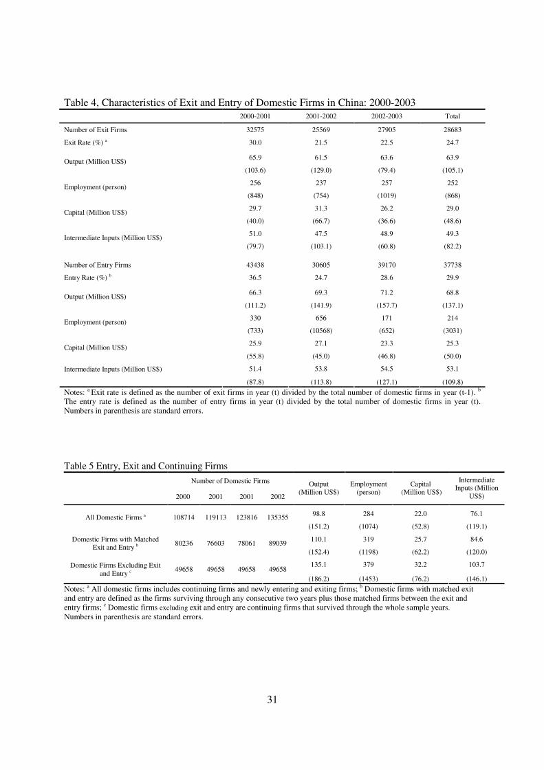
There was substantial entry and exit in our sample period. As is shown in Table 4, the average

entry rate and exit rate of domestic firms in China are 29.9 percent and 24.6 percent, respectively,

between 2000 and 2004. Although it is difficult to address the issue of selection bias, as pointed

out by (Haskel et al., 2007), we believe it is interesting to consider the exit and entry of domestic

firms in estimating the relationship between FDI and productivity.

To control for the productivity differences between entering and exiting firms, we apply the

neighborhood-matching technique to match entering and exiting firms with similar productivity

levels in the two-digit industries and in three regions (including Eastern China, Middle China

and Western China) for each of the two consecutive years over the whole period of 2000-2003.

Details of implementing the neighborhood-matching technique are in the Appendix A. Throug

this process, three separate data sets are generated: firms that exist throughout the sample period

(continuing firms); firms that have observations in any sample year, thus allowing for free entry

and exit (surviving firms, including continuing firms plus entering and exiting firms); and

surviving firms controlling for the productivity difference of entering and exiting firms. Some

descriptive statistics on the average output, labor, capital, and intermediate inputs, and the

number of observations of the three data sets are summarized in Table 5.

VI. Estimation Results

A. Baseline Specification: output measure

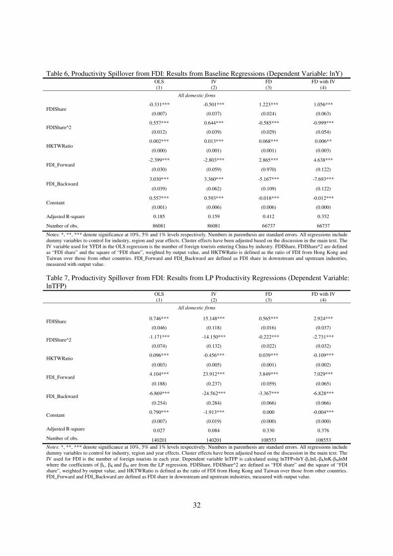
To be consistent with the literature, Table 6 provides the estimates for our baseline-model

specification (Equation (3)) where the dependent variable is the logarithm of output. This

specification is close to that of Aitken and Harrison (1999), Javorick (2004) and Hasket et al.

(2008). The OLS estimates of column (1) affirm the results of Aitken and Harrison (1999),

suggesting that FDI negatively affects the productivity of domestic firms in the same industry.

Moreover, the coefficient of the forward-linkage variable is negative and that of the backward-

18 Less-productive domestic firms usually choose to exit, while the more productive may choose to enter (Helpman, 2006).

18

linkage variable is positive, and both are statistically significant (α = 0.01). This result is

consistent with Javorick (2004), in that positive spillovers from FDI take place through backward

linkage rather than forward linkage.

Using OLS, however, risks encountering two potential problems: (1) the simultaneous-bias

problem wherein FDI may occur in more (or less) productive industries; and (2) the omitted-

variable problem wherein unobserved factors are present in the industry that are closely

correlated with FDI and that affect domestic productivity. The rest of Table 6 contains the results

of regressions that address these identification problems. First, we run OLS but use the number

of foreign visitors as an instrument for FDI (OLS with IV). Second, we repeat OLS but with first

differences (FD). Third, we estimate first-difference regressions with the foreign-visitor

instrument (FD with IV). Columns 2, 3 and 4 in Table 6 report the results from these three

regressions. Removing these identification problems overturns the OLS results of column (1). In

particular, the results from FD and FD with IV consistently indicate that while foreign

investment positively affects same-industry productivity, the effects decrease as the level of FDI

increases, which suggests that the spillover effects of FDI are not monotonic. Rather, the

spillover effects would appear to follow an inverted-U shape. Moreover, vertical spillovers occur

when foreign affiliates supply inputs and equipment to local firms (i.e., through forward linkage

rather than backward linkage), a result that differs from that of Javorick (2004). We also find that

relative to Western firms in China, firms from Hong Kong and Taiwan have a bigger impact on

domestic firms, with the only exception being for the OLS estimates with first differencing. All

effects are statistically significant (α = 0.10).

B. Accounting for Endogeneity of Input Choices: TFP Measure

Although Aitken and Harrison (1999) argue that a regression of output on FDI that controls for

inputs allows for an estimate of productivity, the endogeneity of input choices may be a threat to

identification. Table 7 reports a set of results from regressions using TFP as the dependent

variable, where TFP is derived using the method described in section II. With productivity as the

dependent variable, OLS (Column 1) yields positive and statistically-significant coefficients (α

=0.01) for FDI, suggesting that removing the problem of endogeneity of input choices is

important. Again, the effects decline as the level of FDI increases.

19

Vertical spillovers occur through forward linkage rather than backward linkage and firms from

Hong Kong and Taiwan have bigger spillovers than do Western firms. Accounting further for

problems of simultaneous bias and omitted variables using first differencing together with an

instrumental variable provides even stronger results than those obtained using OLS. This is

shown in columns (2), (3) and (4) of Table 7. The coefficient for FDI is higher and statistically

more significant, as is the case for the square terms of FDI and other vertical variables (forward

and backward linkages). The only exception is the coefficient for the Hong Kong and Taiwan

share, which now turns negative and statistically significant (α = 0.01), suggesting that Western

firms produce more substantive spillovers than do overseas Chinese firms. This is consistent with

observations that the Hong Kong and Taiwan firms that invest in the mainland are usually less

capital intensive and technology advanced than are their Western counterparts, and some of them

are even “round-trip” domestic firms taking advantage of China’s preferential tax treatment for

foreign investors.

C. Firms’ Entry, Exit and FDI Spillovers

Domestic firms’ entry and exit affects the estimation of FDI spillovers in China. Table 3

describes the outputs and inputs of both exiting and entering firms. Note that on average newly-

entering domestic firms have higher outputs and inputs than those exiting, which is again

confirmed in Figure 3 when comparing the productivity distribution between exiting and entering

sample firms.

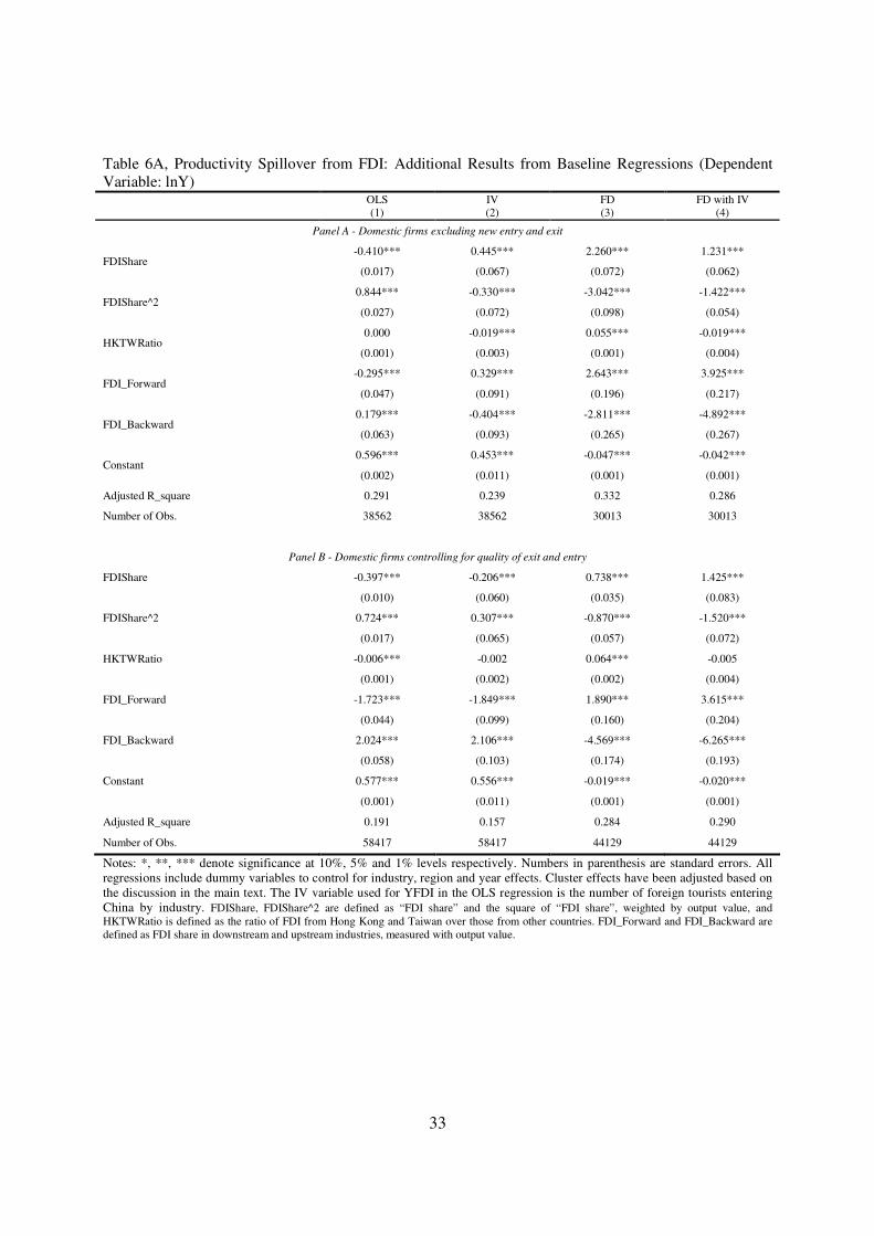
Tables 7 and Panels A and B of 7A provide regression estimates based on the three datasets.19 As

suggested by column (4) of Panel A in Table 7A, excluding entering and exiting firms, a one

percentage point increase in the share of foreign firms in an industry raises the productivity of

continuing firms in the same industry by 0.009 percent and a gain of 0.05 percent for firms in the

downstream industry. Interestingly, when including entering and exiting firms in the sample and

further controlling for productivity differences between entering and exiting firms, the spillover

effects is higher (column (4) of Panel B in Table 7A), suggesting that the productivity spillovers

19 Tables 6 and Panels A and B of 6A provide regression estimates based on the three datasets using output as the dependent variable.

20

(both horizontal and forward spillovers) to entering and exit firms with the similar quality are on

average higher (0.014 and 0.057 percentage points respectively) than spillovers to continuing

firms. Since the coefficient estimate (0.014) implies average spillovers to both continuing firms

and new entrant and exit firms with the similar quality, it indicates that spillovers to new entrant

and exit firms with the similar quality are much higher than 0.014. This is an interesting finding

since the spillovers of foreign firms fall disproportionally on domestic firms, with spillovers to

new entrant and exit firms more than double that to incumbent firms. This result survives even if

there is no control for quality differences among exiting and entering firms. Without controlling

for productivity differences between entering and exiting firms, productivity spillovers to

entering and exiting firms would be even higher that to incumbent firms, as shown in column (4)

of Table 7.

Controlling for firm turnover due to FDI presence re-confirms our results that foreign investment

positively affects the productivity of domestic firms in the same industry. A one percentage point

increase in the share of foreign firms in an industry leads to a 0.015 percent productivity gain for

domestic firms in the same industry and a 0.057 percent productivity gain for domestic firms in

downstream industries.

Figure 2 illustrates the simulated relationship between FDI share in an industry and domestic-

firm productivity using the estimated coefficients as a proxy for FDI share and its square. The

dotted, solid, and dash lines show the result for three scenarios: continuing firms, all firms (with

control for the quality of entering and exiting firms), and surviving firms. For all three scenarios,

the positive spillovers of FDI will reach their maxima when the FDI share in an industry is

approximately 50 percent. This threshold level of FDI is well below the average of our dataset,

suggesting that for most industries in China an increase in FDI will still yield positive spillovers

for domestic firms. Yet, the marginal impacts of FDI on domestic productivity are substantially

different in magnitude across different scenarios. The maximum marginal impact of FDI to the

continuing firms’ productivity is estimated at 0.25 percent, while when considering all firms and

controlling for the quality of entering and exiting firms it becomes 0.36 percent, and for

surviving firms it is 0.78 percent.

21

In terms of the backward-linkage and forward-linkage channels, the pattern of FDI’s impact on

domestic firms’ productivity remains unchanged. The coefficients for the forward-linkage

variable under the four different specifications (OLS, IV, FD, FD with IV) in panel B of Table

7A remain positive and statistically significant (α = 0.01), while the coefficients for the

backward-linkage variable under the four different specifications remain negative and

statistically significant (α = 0.01). But the coefficient for the relative impact of overseas Chinese

firms turns negative for the cases of IV and FD with IV, while remaining positive for the

regression using OLS and FD.

D. Robustness

We provide several robustness checks. It is sometimes argued that the increase in measured

productivity may reflect the degree of concentration in the industry (changes in mark-ups). To

determine whether our estimated coefficients on spillovers to productivity pickup any of the

effects of the industry’s mark-ups, we include a Herfindahl concentration index, defined as the

output share of the top eight firms in each industry. The inclusion of a Herfindahl concentration

index does not affect any of the coefficients.20

We also experiment with an alternative measure of FDI that uses each firm’s share of capital in

the industry as the weight (KFDI). The results are qualitatively the same as using an output-share

measure of FDI.

We test for potential specification problems by estimating regressions with and without the

square FDI term. The results indicate that the hypothesis that only the FDI share enters the

regression but not its square can be rejected (α = 0.01) in most regressions, which implies that

the inverted “U” shape of FDI spillovers fits better than a linear curve.

Taken together, our results suggest that FDI has a significant positive impact on domestic firms’

productivity within the same industry, which declines as the level of FDI increases. We find that

positive spillovers are more likely to occur through forward linkage where domestic firms

20 The results from the robust checks are not reported here due to space, but are available on request.

22

purchase high-quality intermediate inputs or equipment from foreign suppliers than through

backward linkage where they produce for multinationals.

E. Export-orientation, ownership and FDI spillovers

The above results suggest that on average domestic firms do benefit from FDI. Yet one may be

interested in whether this observation masks heterogeneity across different types of firms. In this

section we consider the relationship between three attributes of domestic firms and their benefits

from the presence of foreign firms: namely, export-oriented vs. domestic-market-oriented firms,

large firms vs. small firms and state-owned enterprises (SOEs) vs. non-SOE firms.

Table 8 reports regression results for two set of firms: exporting and non-exporting domestic

firms. The results indicate that whether a firm is exporting or not has significant implications for

their benefits from FDI. For non-exporting domestic firms, the coefficient estimates for both FDI

and forward-linkage variables are positive and significant, and are robust across the four sets of

specifications, suggesting that non-exporting domestic firms benefit from FDI in the same

industry as well as in their upstream industry (forward linkage). In contrast, for exporting firms,

the coefficient estimates for FDI, and the forward and backward linkage variables are all

negative and significant, suggesting that exporting firms are adversely affected by FDI firms.

Whether a firm is state-owned also affects the spillover effects of FDI. For non-SOE firms, the

coefficient estimates for both FDI and forward-linkage variables are positive and significant and

robust across different sets of specifications, suggesting that non-SOE firms accrue greater

benefit from FDI than do SOEs (Table 9).

As shown in Table 10, the coefficients for the FDI and forward-linkage variables are positive and

significant for firms with different sizes, but large and medium firms enjoyed greater benefits

from FDI than did small firms, in particular through forward linkage. Taken together, domestic

firms differ significantly in the extent to which they benefit from FDI, with large, non-exporting

and non-SOE firms accruing the greatest benefits from foreign firms in China.

23

V. Conclusion

China has emerged as the largest recipient of foreign direct investment (FDI) in the developing

world, yet little is known about the benefits for domestic firms. Using firm-level census data

from China for the period of 2000-2003, this paper examines the various channels of FDI

spillovers. We find that FDI have had a significant positive impact on domestic productivity

within the same industry, but the benefits decline as the level of FDI increases. More importantly,

we are able to identify sizable gains in productivity spillovers arising from firms’ turnover (entry

and exit). We find that the spillovers of foreign firms fall disproportionally on firms, with

spillovers to new entrant and exit firms more than double that to existing firms.

We also find substantial vertical spillovers, which are more likely to happen through forward

linkage than through backward linkage. Moreover, firms in China do not benefit uniformly from

foreign investment, with large, non-exporting and non-SOE firms accruing the greatest benefits

from foreing presence in China.

The positive spillovers to domestic firms from FDI suggest that Chinese governments

preferential treatments for forieng firms in past decades may be justifiable. However, the

negative backward linkage effect we identified in this paper requires more policy attention. For a

long time the Chinese government provides tax incentives to attract foreign investmnet (such as

exemption of import duty to those firms that import equipment and inputs, provided that those

firms exported their goods to international market), for fear of a shortage of foreign exchange,.

This export incentive, although successful in encouraging exports, comes with an implicit cost

by reducing the incentive for domestic firms to supply parts, intermediate inputs and equipment

to forieng firms. Now that China’s foreign exchange reserves have reached to about US$2

trillion, concerns about shortage of foreign exchange are remote and a rethinking of tax incentive

may be warranted. Further, our result that entering and exiting firms benefit more from FDI than

existing firms suggests that moving towards a market environment could benefit society by

stimulating further entry and exit.

24

However, notwithstanding the government policy, the benefits from FDI are not automatic, but

require some support from domestic firms also. Perhaps, more R&D is needed to increase the

quality of domestic products to attract foreign firms to source products from the domestic market.

Furthermore, as non-SOE firms accrue greater benefits from foreign firms in China than SOE

firms, there is an incentive to continue reform of SOEs.

Reference

Aitken, B. and A. Harrison (1999) Do Domestic Firms Benefit from Foreign Direct Investment? Evidence from Panel Data. American Economic Review, 89(3): 605-618. Aw, Bee Yan, Xiaomin Chen and Mark Roberts (2001) Firm-Level Evidence on Productivity Differentials and Turnover in Taiwanese Manufacturing, Journal of Development Economics, 66: 51-86. Bertrand M., E. Duflo and S. Mullainathan (2004) How Much Should We Trust Differences-In-Differences Estimates?, Quarterly Journal of Economics 119(1), pp. 249–276. Blalock, G. and P. J. Gertler (2007) Welfare gains from Foreign Direct Investment through Technology Transfer to Local Suppliers, Journal of International Economics, Vol. 74 No.2, pp.402-421. Findlay, R. (1978) Relative Backwardness, Direct Foreign Investment, and the Trans-fer of Technology: A Simple Dynamic Model, Quarterly Journal of Economics, 92(1): pp.1-16. Griffith, R., R. Harrison and H. Simpson (2006) The link between Product Market Reform, Innovation and EU Macroeconomic Performance, Economic Papers, No. 243, ECFIN Brusssels. Hahn, J., P. Todd and W. Van der Klaauw (2001) Identification and Estimation of Treatment Effects with a Regression-Discontinuity Design, Econometrica, 69(1), pp. 201-209. Hale, Galina and Cheryl Long (2007) Are There Productivity Spillovers from Foreign Direct Investment in China? Federal reserve bank of san francisco Working paper series. Haskel, J. E., S. Pereira and M. Slaughter (2007) Does Inward Foreign Direct Investment Boost the Productivity of Domestic Firms? Review of Economics and Statistics, 89(3): pp.482-496. Helpman, E. (2006) Trade, FDI and the Organization of Firms, Journal of Economic Literature, 44(3) pp. 589-630. Hu, A. G. and G. H. Jefferson (2002) FDI Impact and Spillover: Evidence from China’s Electronic and Textile Industries, The World Economy, 25, 1063–1076.

25

Imbens, G. W. and J. D. Angrist (1994) Identification and Estimation of Local Average Treatment Effects, Econometrica, 62(2) pp. 467-475. Javorcik, B. S., (2004) Does Foreign Direct Investment Increase the Productivity of Domestic Firms? In Search of Spillovers through Backward Linkages, The American Economic Review, Vol. 94, No. 3, pp. 605-627. Klette, Tor Jacob and Zvi Griliches (1996) The Inconsistency of Common Scale Estimators When Output Prices are Unobserved and Endogenous. Journal of Applied Econometrics, 11(4): 343-61. Leuven, E. and B. Sianesi (2008) PSMATCH2: Stata Module to Perform Full Mahalanobis and Propensity Score Matching, Common Support Graphing, and Covariate Imbalance Testing, IDEAS Working Paper, available at the website: http://ideas.repec.org/c/boc/bocode/s432001.html#abstract. Levinsohn, J. and A. Petrin (2003) Estimating Production Functions Using Inputs to Control for Unobservables, Reviews of Economic Studies, 70(2), pp.317-342. Moulton, B. R. (1990) An Illustration of a Pitfall in Estimating the Effects of Aggregate Variables on Micro Units, The Review of Economics and Statistics, 72(2) pp. 334-338. Olley, S. G. and A. Pakes (1996) The Dynamics of Productivity in the Telecommunications Equipment Industry, Econometrica, 64(4), pp. 1263-1297. Rodrik, Dani (1999) The New Global Economy and Developing Countries: Making Openness Work.” Overseas Development Council (Baltimore, ND) Policy Essay No. 24. Rosenbaum, P. R., and Rubin, D. B. (1983) The Central Role of the Propensity Score in Observational Studies for Causal Effects, Biometrika 70, pp.41-55. Sun, Q, W. Tong and Q. Yu (2002) Determinants of foreign direct investment across China, Journal of International Money and Finance, 21(1): pp.79-113. Woodridge, J. (2006) Cluster-sample methods in applied econometrics: An Extended Analysis, mimeo, website: https://www.msu.edu/~ec/faculty/wooldridge/current%20research/clus1aea.pdf

UNCTAD (2008) World Investment Reports 2008. United Nations Conference for Trade and Development.

26

Appendix A. Neighborhood matching between entering and exiting firms with similar productivity To control for differences in productivity between entering and exiting domestic firms, we adopt

a neighborhood-matching technique based on propensity score estimation (Imbens and Angrist,

1994 and Hahn, Todd and Klaauw, 2001 and Leuven and Sianesi, 2008). Although entering and

exiting firms have productivity, firms from both groups can be treated as similarif their inputs

and outputs are controlled for. As long as we can separate the similar firms from non-similar

firms based on the neighborhood-matching technique, selection bias due to firms’ entry and exit

can be controlled.

To do so, we define two groups (the entering and exiting firms) in different industries (at 2-digit

ISIC level) and regions (including the East, Middle and West region) for each of two consecutive

years, and assume switching between the two groups as a type of treatment. Thus, we have one

of the two groups (i.e. entering firms) as the treated group (or 1=T ), while the other as the non-

treated one (or 0=T ). Based on the literature on “treatment effects”, we further assume that (1)

all relevant difference in productivity between the two group firms are captured by the observed

firms’ output and inputs since we are interested in their productivity differences across groups

(which is determined by the input and output relationship); (2) the distribution of observed

output and inputs in the controlled group selected from the non-treated pool, is as similar as the

distribution in the treated group (since each firm is randomly selected).21 The conditional

probability of treatment (say, a firm switching from exiting to entering status) given the

background variables for each individual firm can be defined as (Rosenbaum and Rubin, 1983):

|1Pr)( xXTxpdef

=== (A1)

where )(xp is the conditional probability or the so-called propensity score, T is the binary

treatment and )int,,,( nputsermediateicapitallabouroutputX = are firms’ output and inputs (or

the background variables). As is proved in Rosenbaum and Rubin (1983),

XTFPTFPT |)1(),0(|⊥ is equal to )(|)1(),0(| xpTFPTFPT ⊥ if un-confoundedness holds. This

21 These assumptions guarantee that the neighbourhood matching is performed over the common support region.

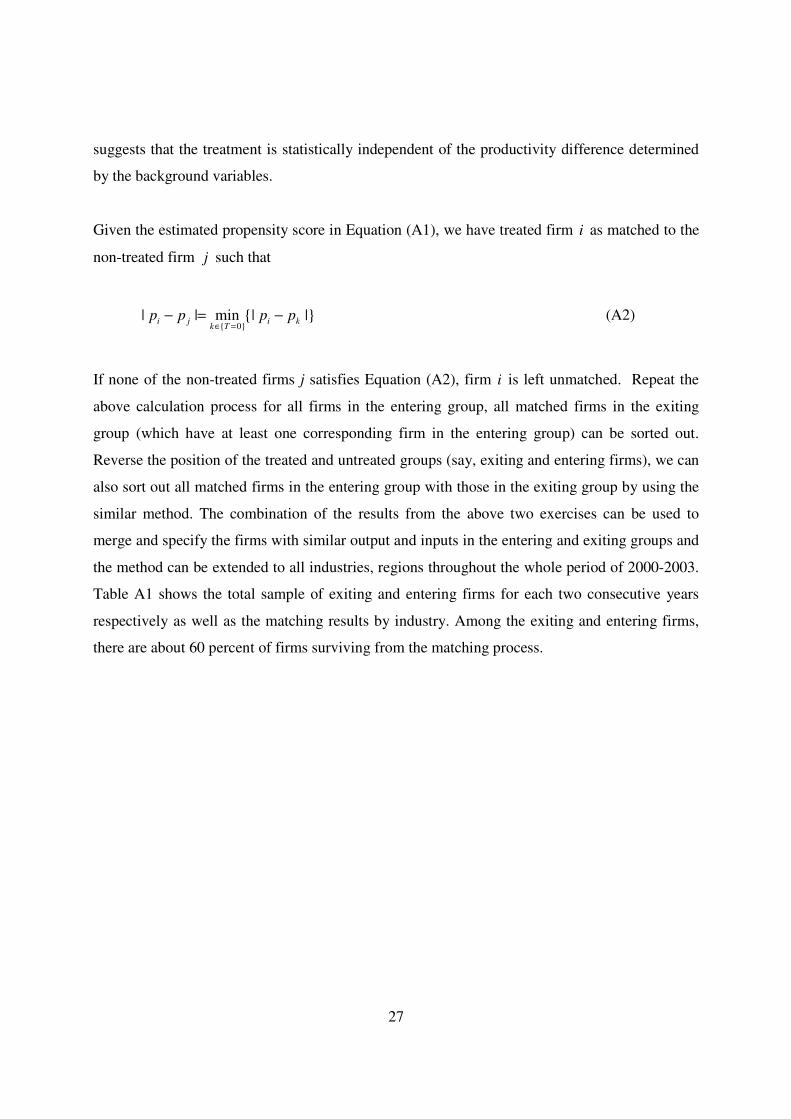
27

suggests that the treatment is statistically independent of the productivity difference determined

by the background variables.

Given the estimated propensity score in Equation (A1), we have treated firm i as matched to the

non-treated firm j such that

||min||0

kiTk

ji pppp −=−=∈

(A2)

If none of the non-treated firms j satisfies Equation (A2), firm i is left unmatched. Repeat the

above calculation process for all firms in the entering group, all matched firms in the exiting

group (which have at least one corresponding firm in the entering group) can be sorted out.

Reverse the position of the treated and untreated groups (say, exiting and entering firms), we can

also sort out all matched firms in the entering group with those in the exiting group by using the

similar method. The combination of the results from the above two exercises can be used to

merge and specify the firms with similar output and inputs in the entering and exiting groups and

the method can be extended to all industries, regions throughout the whole period of 2000-2003.

Table A1 shows the total sample of exiting and entering firms for each two consecutive years

respectively as well as the matching results by industry. Among the exiting and entering firms,

there are about 60 percent of firms surviving from the matching process.

28

Table 1, Summary Statistics for Domestic and FDI firms in China: 2000-2003

2000 2001 2002 2003

Total Domestic FDI Total Domestic FDI Total Domestic FDI Total Domestic FDI

106.2 86.2 191.3 112.5 89.4 208.5 126.6 101.0 231.8 148.5 115.3 279.1 Output (million US$)

(150.4) (120.9) (237.1) (187.5) (128.47) (334.8) (214.4) (148.5) (379.3) (288.3) (189.4) (519.9)

315 313 324 336 332 354 365 362 382 276 259 345 Employment (person)

(1182) (1248) (859) (1249) (1335) (886) (2461) (2766) (962) (921) (957) (756)

46.2 40.4 70.4 46.7 40.3 72.7 47.9 41.4 74.4 47.3 40.5 73.9 Capital (million US$)

(73.4) (70.5) (82.1) (89.9) (83.1) (109.5) (94.6) (91.4) (105.9) (84.8) (78.8) (102.3)

82.5 66.4 150.6 87.6 69.2 163.7 97.9 77.7 180.8 114.5 88.1 218.4 Intermediate Inputs (million US$)

(121.5) (93.7) (199.6) (149.7) (102.2) (267.2) (172.9) (117.5) (309.3) (238.2) (148.6) (440.6)

21.7 22.8 23.2 24.1 Horizontal FDI Share (%)

(10.7) - -

(11.2) - -

(11.2) - -

(11.7) - -

44.2 44.6 43.2 43.5 HKTW Share in FDI (%)

(11.9) - -

(14.1) - -

(13.2) - -

(15.4) - -

8.5 8.8 9.0 9.5 Upstream FDI Share (%)

(6.2) - -

(6.3) - -

(6.5) - -

(6.8) - -

6.7 7.0 7.1 7.5 Downstream FDI Share (%)

(4.8) - -

(4.9) - -

(4.9) - -

(5.2) - -

Number of Firms 134130 108714 25416 147690 119113 28577 154317 123816 30501 169810 135355 34455

Note: Output is defined as the total output value, employment is defined as the total number of employees, and capital is defined as the net fixed asset value. All financial variables are measured with US dollars at the 1990 constant price, and the exchange rate used for the conversion is 4.7832 (China Statistical Yearbook, 2000, 2001, 2002, 2003). Numbers in parenthesis are standard errors.

29

Table 2, FDI Share (Output weighted) by Industry in China: 2000-2003 (Unit: Percent)

2000 2001 2002 2003 Total Sector ID

Sector Name FDI

Share

Num. of FDI Firms

FDI Share

Num. of FDI Firms

FDI Share

Num. of FDI Firms

FDI Share

Num. of FDI Firms

FDI Share

Num. of FDI Firms

13 Food Processing 16.8 [1017] 17.9 [1154] 17.5 [1225] 17.3 [1377] 17.4 [1193]

14 Food Production 29.3 [765] 33.2 [823] 30.5 [876] 30.7 [951] 30.9 [854] 15 Beverage Production 24.2 [380] 26 [404] 27.9 [406] 30.2 [460] 27.1 [413] 16 Tobacco Processing 0.1 [4] 0.3 [4] 0.2 [4] 0.2 [6] 0.2 [5] 17 Textile industry 14.1 [2003] 15.1 [2274] 15.5 [2450] 17 [2812] 15.5 [2385]

18 Clothing and Footware 33.7 [2705] 33.7 [2984] 33.2 [3203] 34.7 [3670] 33.8 [3141]

19 Leather, Fur, Feather and Related Products

43 [1153] 40.6 [1305] 39.5 [1423] 39.9 [1658] 40.6 [1385]

20 Timber Processing, Wood, Bamboo, Rattan, Palm and Straw Products

18.5 [453] 20.1 [531] 19.1 [529] 20.7 [610] 19.7 [531]

21 Furniture Manufacturing 34.5 [399] 35.4 [436] 36.5 [479] 40.9 [548] 37.1 [466]

22 Paper and Paper Products 23.6 [631] 23.8 [684] 25 [688] 23.7 [741] 24 [686]

23 Printing and Medium Reproduction

20.5 [442] 23.2 [488] 22.8 [504] 23.8 [556] 22.6 [498]

24 Cultural, Educational and Sports Goods

48.3 [770] 48.3 [820] 49.3 [917] 51 [1131] 49.4 [910]

25 Petroleum refining, Coking, and Gas Production and Supply

4.8 [112] 4.5 [89] 7.6 [121] 7.1 [92] 6.2 [104]

26 Raw Chemical Materials and Chemical Products

15.4 [1274] 16.5 [1502] 17.4 [1596] 19.6 [1850] 17.4 [1556]

27 Medical and Pharmaceutical Products

13.5 [464] 12.3 [554] 13.3 [545] 13 [597] 13 [540]

28 Chemical Fibers 21.5 [164] 16 [154] 17 [162] 13.8 [181] 16.8 [165] 29 Rubber Products 25.6 [319] 25.8 [348] 28.4 [342] 27.2 [393] 26.8 [351] 30 Plastics Products 33.2 [1730] 32.3 [1914] 31.2 [2010] 33 [2194] 32.4 [1962]

31 Nonferrous Mineral Products 12.3 [1245] 13.1 [1402] 12.9 [1445] 11.9 [1553] 12.6 [1411]

32 Smelting and Pressing of Ferrous Metals

5.1 [198] 5.6 [223] 6.3 [223] 7 [245] 6 [222]

33 Smelting and Pressing of Non-ferrous Metals

7.7 [213] 8.3 [188] 8.2 [222] 9.5 [309] 8.5 [233]

34 Metal Products 27.8 [1336] 26.2 [1525] 26.3 [1616] 26 [1756] 26.5 [1558]

35 General Purpose Machinery 15.9 [961] 15.2 [1093] 16.3 [1235] 18.8 [1592] 16.7 [1220]

36 Special Purpose Machinery 10.6 [651] 13.7 [810] 12.8 [823] 14.9 [929] 13.1 [803]

37 Transportion Equipment 20 [865] 20.9 [998] 20.4 [1103] 22.5 [1224] 21 [1048]

39 Electrical Machinery and Equipment

25.1 [1578] 26.4 [1819] 27.1 [1963] 28 [2163] 26.7 [1881]

40 Communication Equipment, Computers and Other Electronic Equipment

47.7 [1927] 55.1 [2167] 56.3 [2352] 59.9 [2712] 55.2 [2290]

41 Instruments, Meters, Cultural and Clerical Machinery

53.6 [542] 58.9 [608] 57.9 [628] 60.1 [781] 57.9 [640]

42 Other Manufacturing 32.6 [1115] 32.1 [1276] 35.1 [1411] 31.1 [1364] 32.8 [1292]

Total All Manufacture 21.7 [25416] 22.8 [28577] 23.2 [30501] 24.1 [34455] 23 [29737]

Note: Numbers in the rectangle parenthesis are number of foreign firms.

30

Table 3, Comparison of Productivity Estimates between OLS and LP Methods

Panel A Panel B Panel C

Coefficients from OLS Regressiona Coefficients from LP Regressionb Sign Change between A and Bc Sector ID

Number of Obs.

lnL lnK lnM lnL lnK lnM ∆lnL ∆lnK ∆lnM

13 33645 0.064*** 0.001 0.905*** 0.043*** 0.021*** 0.700*** - + -

14 11875 0.017*** 0.003** 0.971*** 0.014*** 0.025*** 0.794*** - + -

15 9256 0.036*** 0.008*** 0.963*** 0.03*** 0.029* 0.700*** - + -

16 973 0.055*** 0.068*** 0.965*** 0.028* Nil Nil - Nil Nil

17 36238 0.032*** 0.009*** 0.947*** 0.032*** 0.003 0.872*** - - -

18 17276 0.047*** 0.015*** 0.935*** 0.044*** 0.009 0.904*** - - -

19 8152 0.032*** 0.013*** 0.943*** 0.029*** 0.013* 0.968*** - - +

20 8622 0.037*** 0.005*** 0.95*** 0.039*** 0.001 0.856*** + - -

21 4280 0.031*** 0.012*** 0.953*** 0.032*** 0.000 1.000*** + - +

22 15062 0.03*** 0.008*** 0.952*** 0.031*** 0.004 0.870*** + - -

23 11364 0.045*** 0.023*** 0.933*** 0.038*** Nil Nil - Nil Nil

24 3881 0.034*** 0.015*** 0.943*** 0.035*** 0.010 0.820*** + - -

25 3889 0.021*** 0.014*** 0.949*** 0.024*** 0.018 0.966*** + + +

26 35311 0.025*** 0.01*** 0.952*** 0.024*** 0.000 0.973*** - - +

27 10746 0.042*** 0.019*** 0.942*** 0.035*** 0.03*** 0.858*** - + -

28 2031 0.028*** 0.005* 0.955*** 0.029*** 0.014* 0.856*** + + -

29 5146 0.033*** 0.012*** 0.945*** 0.031*** 0.003 0.972*** - - +

30 18391 0.037*** 0.013*** 0.944*** 0.033*** 0.015*** 0.951*** - + +

31 47133 0.033*** 0.004*** 0.951*** 0.031*** 0.003 0.87*** - - -

32 11434 0.029*** 0.004*** 0.959*** 0.03*** 0.009 0.958*** + + -

33 8246 0.04*** 0.006*** 0.948*** 0.041*** 0.013 0.953*** + + +

34 24019 0.035*** 0.015*** 0.94*** 0.032*** 0.013* 0.844*** - - -

35 33076 0.037*** 0.01*** 0.944*** 0.036*** 0.000 1.000*** - - +

36 19825 0.022*** 0.006*** 0.957*** 0.024*** 0.016*** 0.978*** + + +

37 21729 0.042*** 0.01*** 0.939*** 0.037*** 0.015** 0.915*** - + -

39 25830 0.031*** 0.012*** 0.952*** 0.029*** Nil Nil - Nil Nil

40 9082 0.049*** 0.013*** 0.944*** 0.04*** 0.018 0.830*** - + -

41 5038 0.052*** 0.005*** 0.94*** 0.053*** 0.007 0.938*** + + -

42 9864 0.045*** 0.013*** 0.935*** 0.044*** 0.000 1.000*** - - +

Note: a The regression is based on the OLS method with random effects. b The regression is based on the LP method, which is a semi-parametric GMM estimate (See Olley and Pakes, 1996; Levinsohn and Petrin, 2003). c The sign comes from the estimates from the LP method minus the estimates from the OLS method. d * represents significant at 10 percent level, ** represents significant at 5 percent level and *** represents significant at 1 percent level.

31

Table 4, Characteristics of Exit and Entry of Domestic Firms in China: 2000-2003 2000-2001 2001-2002 2002-2003 Total

Number of Exit Firms 32575 25569 27905 28683

Exit Rate (%) a 30.0 21.5 22.5 24.7

65.9 61.5 63.6 63.9 Output (Million US$)

(103.6) (129.0) (79.4) (105.1)

256 237 257 252 Employment (person)

(848) (754) (1019) (868)

29.7 31.3 26.2 29.0 Capital (Million US$)

(40.0) (66.7) (36.6) (48.6)

51.0 47.5 48.9 49.3 Intermediate Inputs (Million US$)

(79.7) (103.1) (60.8) (82.2)

Number of Entry Firms 43438 30605 39170 37738

Entry Rate (%) b 36.5 24.7 28.6 29.9

66.3 69.3 71.2 68.8 Output (Million US$)

(111.2) (141.9) (157.7) (137.1)

330 656 171 214 Employment (person)

(733) (10568) (652) (3031)

25.9 27.1 23.3 25.3 Capital (Million US$)

(55.8) (45.0) (46.8) (50.0)

51.4 53.8 54.5 53.1 Intermediate Inputs (Million US$) (87.8) (113.8) (127.1) (109.8)

Notes: a Exit rate is defined as the number of exit firms in year (t) divided by the total number of domestic firms in year (t-1). b

The entry rate is defined as the number of entry firms in year (t) divided by the total number of domestic firms in year (t). Numbers in parenthesis are standard errors.

Table 5 Entry, Exit and Continuing Firms

Number of Domestic Firms

2000 2001 2001 2002

Output (Million US$)

Employment (person)

Capital (Million US$)

Intermediate Inputs (Million

US$)

98.8 284 22.0 76.1 All Domestic Firms a 108714 119113 123816 135355

(151.2) (1074) (52.8) (119.1)

110.1 319 25.7 84.6 Domestic Firms with Matched Exit and Entry b

80236 76603 78061 89039

(152.4) (1198) (62.2) (120.0)

135.1 379 32.2 103.7 Domestic Firms Excluding Exit and Entry c

49658 49658 49658 49658

(186.2) (1453) (76.2) (146.1)

Notes: a All domestic firms includes continuing firms and newly entering and exiting firms; b Domestic firms with matched exit and entry are defined as the firms surviving through any consecutive two years plus those matched firms between the exit and entry firms; c Domestic firms excluding exit and entry are continuing firms that survived through the whole sample years. Numbers in parenthesis are standard errors.

32

Table 6, Productivity Spillover from FDI: Results from Baseline Regressions (Dependent Variable: lnY)

OLS (1)

IV (2)

FD (3)

FD with IV (4)

All domestic firms

-0.331*** -0.501*** 1.223*** 1.056*** FDIShare

(0.007) (0.037) (0.024) (0.063)

0.557*** 0.644*** -0.585*** -0.999*** FDIShare^2

(0.012) (0.039) (0.029) (0.054)

0.002*** 0.013*** 0.068*** 0.006** HKTWRatio

(0.000) (0.001) (0.001) (0.003)

-2.399*** -2.803*** 2.865*** 4.638*** FDI_Forward

(0.030) (0.059) (0.970) (0.122)

3.030*** 3.360*** -5.167*** -7.693*** FDI_Backward

(0.039) (0.062) (0.109) (0.122)

0.557*** 0.593*** -0.018*** -0.012*** Constant

(0.001) (0.006) (0.006) (0.000)

Adjusted R-square 0.185 0.159 0.412 0.352

Number of obs. 86081 86081 66737 66737

Notes: *, **, *** denote significance at 10%, 5% and 1% levels respectively. Numbers in parenthesis are standard errors. All regressions include dummy variables to control for industry, region and year effects. Cluster effects have been adjusted based on the discussion in the main text. The IV variable used for YFDI in the OLS regression is the number of foreign tourists entering China by industry. FDIShare, FDIShare^2 are defined as “FDI share” and the square of “FDI share”, weighted by output value, and HKTWRatio is defined as the ratio of FDI from Hong Kong and Taiwan over those from other countries. FDI_Forward and FDI_Backward are defined as FDI share in downstream and upstream industries, measured with output value.

Table 7, Productivity Spillover from FDI: Results from LP Productivity Regressions (Dependent Variable: lnTFP)

OLS (1)

IV (2)

FD (3)

FD with IV (4)

All domestic firms

0.746*** 15.148*** 0.565*** 2.924*** FDIShare

(0.046) (0.118) (0.016) (0.037)

-1.171*** -14.150*** -0.222*** -2.731*** FDIShare^2

(0.074) (0.132) (0.022) (0.032)

0.096*** -0.456*** 0.039*** -0.109*** HKTWRatio

(0.003) (0.005) (0.001) (0.002)

4.104*** 23.912*** 3.849*** 7.029*** FDI_Forward

(0.188) (0.237) (0.059) (0.065)

-6.869*** -24.562*** -3.367*** -6.828*** FDI_Backward

(0.254) (0.284) (0.066) (0.066)

0.790*** -1.913*** 0.000 -0.004*** Constant

(0.007) (0.019) (0.000) (0.000)

Adjusted R-square 0.027 0.084 0.330 0.376

Number of obs. 140201 140201 108553 108553

Notes: *, **, *** denote significance at 10%, 5% and 1% levels respectively. Numbers in parenthesis are standard errors. All regressions include dummy variables to control for industry, region and year effects. Cluster effects have been adjusted based on the discussion in the main text. The IV used for FDI is the number of foreign tourists in each year. Dependent variable lnTFP is calculated using lnTFP=lnY-βLlnL-βKlnK-βMlnM where the coefficients of βL, βK and βM are from the LP regression. FDIShare, FDIShare^2 are defined as “FDI share” and the square of “FDI share”, weighted by output value, and HKTWRatio is defined as the ratio of FDI from Hong Kong and Taiwan over those from other countries. FDI_Forward and FDI_Backward are defined as FDI share in downstream and upstream industries, measured with output value.

33

Table 6A, Productivity Spillover from FDI: Additional Results from Baseline Regressions (Dependent Variable: lnY)

OLS (1)

IV (2)

FD (3)

FD with IV (4)

Panel A - Domestic firms excluding new entry and exit

-0.410*** 0.445*** 2.260*** 1.231*** FDIShare

(0.017) (0.067) (0.072) (0.062)

0.844*** -0.330*** -3.042*** -1.422*** FDIShare^2

(0.027) (0.072) (0.098) (0.054)

0.000 -0.019*** 0.055*** -0.019*** HKTWRatio

(0.001) (0.003) (0.001) (0.004)

-0.295*** 0.329*** 2.643*** 3.925*** FDI_Forward

(0.047) (0.091) (0.196) (0.217)

0.179*** -0.404*** -2.811*** -4.892*** FDI_Backward

(0.063) (0.093) (0.265) (0.267)

0.596*** 0.453*** -0.047*** -0.042*** Constant

(0.002) (0.011) (0.001) (0.001)

Adjusted R_square 0.291 0.239 0.332 0.286

Number of Obs. 38562 38562 30013 30013

Panel B - Domestic firms controlling for quality of exit and entry

FDIShare -0.397*** -0.206*** 0.738*** 1.425***

(0.010) (0.060) (0.035) (0.083)

FDIShare^2 0.724*** 0.307*** -0.870*** -1.520***

(0.017) (0.065) (0.057) (0.072)

HKTWRatio -0.006*** -0.002 0.064*** -0.005

(0.001) (0.002) (0.002) (0.004)

FDI_Forward -1.723*** -1.849*** 1.890*** 3.615***

(0.044) (0.099) (0.160) (0.204)

FDI_Backward 2.024*** 2.106*** -4.569*** -6.265***

(0.058) (0.103) (0.174) (0.193)

Constant 0.577*** 0.556*** -0.019*** -0.020***

(0.001) (0.011) (0.001) (0.001)

Adjusted R_square 0.191 0.157 0.284 0.290

Number of Obs. 58417 58417 44129 44129

Notes: *, **, *** denote significance at 10%, 5% and 1% levels respectively. Numbers in parenthesis are standard errors. All regressions include dummy variables to control for industry, region and year effects. Cluster effects have been adjusted based on the discussion in the main text. The IV variable used for YFDI in the OLS regression is the number of foreign tourists entering China by industry. FDIShare, FDIShare^2 are defined as “FDI share” and the square of “FDI share”, weighted by output value, and HKTWRatio is defined as the ratio of FDI from Hong Kong and Taiwan over those from other countries. FDI_Forward and FDI_Backward are defined as FDI share in downstream and upstream industries, measured with output value.

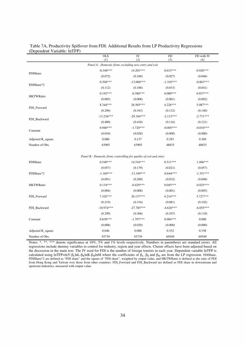
34

Table 7A, Productivity Spillover from FDI: Additional Results from LP Productivity Regressions (Dependent Variable: lnTFP)

OLS (1)

IV (2)

FD (3)

FD with IV (4)

Panel A - Domestic firms excluding new entry and exit

-0.348*** 14.291*** 0.633*** 0.920*** FDIShare

(0.072) (0.168) (0.027) (0.046)

0.304*** -13.060*** -1.105*** -0.863*** FDIShare^2

(0.112) (0.188) (0.033) (0.041)

0.192*** -0.380*** 0.080*** 0.037*** HKTWRatio

(0.005) (0.008) (0.001) (0.002)

8.344*** 26.565*** 4.226*** 5.087*** FDI_Forward

(0.296) (0.343) (0.132) (0.140)

-13.236*** -29.184*** -2.115*** -2.771*** FDI_Backward

(0.400) (0.418) (0.116) (0.121)

0.940*** -1.720*** -0.005*** -0.010*** Constant

(0.010) (0.028) (0.000) (0.000)

Adjusted R_square 0.080 0.137 0.383 0.369

Number of Obs. 63905 63905 48835 48835

Panel B - Domestic firms controlling for quality of exit and entry

FDIShare 0.540*** 14.516*** 0.511*** 1.406***

(0.057) (0.179) (0.021) (0.057)

FDIShare^2 -1.169*** -13.349*** -0.644*** -1.351***

(0.091) (0.200) (0.032) (0.048)

HKTWRatio 0.134*** -0.429*** 0.045*** -0.025***

(0.004) (0.008) (0.001) (0.003)

FDI_Forward 7.102*** 26.137*** 4.214*** 5.727***

(0.219) (0.316) (0.081) (0.102)

FDI_Backward -10.974*** -27.785*** -4.620*** -6.055***

(0.299) (0.366) (0.107) (0.110)

Constant 0.838*** -1.797*** 0.004*** 0.000

(0.008) (0.029) (0.000) (0.000)

Adjusted R_square 0.046 0.088 0.352 0.358

Number of Obs. 93739 93739 69549 69549

Notes: *, **, *** denote significance at 10%, 5% and 1% levels respectively. Numbers in parenthesis are standard errors. All regressions include dummy variables to control for industry, region and year effects. Cluster effects have been adjusted based on the discussion in the main text. The IV used for FDI is the number of foreign tourists in each year. Dependent variable lnTFP is calculated using lnTFP=lnY-βLlnL-βKlnK-βMlnM where the coefficients of βL, βK and βM are from the LP regression. FDIShare, FDIShare^2 are defined as “FDI share” and the square of “FDI share”, weighted by output value, and HKTWRatio is defined as the ratio of FDI from Hong Kong and Taiwan over those from other countries. FDI_Forward and FDI_Backward are defined as FDI share in downstream and upstream industries, measured with output value.

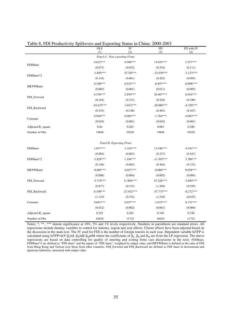
35

Table 8, FDI Productivity Spillovers and Exporting Status in China: 2000-2003

OLS (1)

IV (2)

FD (3)

FD with IV (4)

Panel A - Non-exporting Firms

0.622*** 0.580*** 15.035*** 2.557*** FDIShare

(0.071) (0.032) (0.254) (0.111)

-1.849*** -0.720*** -14.439*** -2.133*** FDIShare^2

(0.118) (0.061) (0.282) (0.095)

0.100*** 0.032*** -0.497*** -0.098*** HKTWRatio

(0.005) (0.001) (0.011) (0.005)

6.536*** 2.859*** 26.407*** 6.016*** FDI_Forward

(0.244) (0.123) (0.420) (0.180)

-10.435*** -3.832*** -28.080*** -6.350*** FDI_Backward

(0.335) (0.148) (0.465) (0.167)

0.944*** 0.004*** -1.764*** -0.003*** Constant

(0.010) (0.001) (0.042) (0.001)

Adjusted R_square 0.04 0.262 0.063 0.280

Number of Obs. 74846 55628 74846 55628

Panel B -Exporting Firms

FDIShare 1.817*** -1.224*** 13.546*** -4.541***

(0.094) (0.063) (0.327) (0.167)

FDIShare^2 -1.828*** 1.104*** -11.303*** 3.706***

(0.148) (0.062) (0.364) (0.152)

HKTWRatio -0.085*** -0.027*** -0.086*** 0.038***

(0.008) (0.004) (0.005) (0.004)

FDI_Forward -5.719*** 11.804*** 47.226*** -3.694***

(0.877) (0.315) (1.269) (0.595)

FDI_Backward 6.100*** -23.442*** -57.775*** -6.272***

(1.119) (0.374) (1.529) (0.625)

Constant 0.601*** 0.037*** -1.835*** 0.132***

(0.012) (0.002) (0.061) (0.004)

Adjusted R_square 0.225 0.285 0.349 0.328

Number of Obs. 44424 11722 44424 11722

Notes: *, **, *** denote significance at 10%, 5% and 1% levels respectively. Numbers in parenthesis are standard errors. All regressions include dummy variables to control for industry, region and year effects. Cluster effects have been adjusted based on the discussion in the main text. The IV used for FDI is the number of foreign tourists in each year. Dependent variable lnTFP is calculated using lnTFP=lnY-βLlnL-βKlnK-βMlnM where the coefficients of βL, βK and βM are from the LP regression. The above regressions are based on data controlling for quality of entering and exiting firms (see discussions in the text). FDIShare, FDIShare^2 are defined as “FDI share” and the square of “FDI share”, weighted by output value, and HKTWRatio is defined as the ratio of FDI from Hong Kong and Taiwan over those from other countries. FDI_Forward and FDI_Backward are defined as FDI share in downstream and upstream industries, measured with output value.

36

Table 9, FDI Productivity Spillovers and Firm Ownership in China: 2000-2003

OLS (1)

IV (2)

FD (3)

FD with IV (4)

Panel A - SOEs Firms

1.323*** 0.048 12.774*** 0.590*** FDIShare

(0.072) (0.034) (0.306) (0.088)

-2.795*** 0.121** -11.715*** -0.690*** FDIShare^2

(0.115) (0.042) (0.337) (0.078)

0.164*** -0.022*** -0.344*** -0.050*** HKTWRatio

(0.005) (0.001) (0.012) (0.005)

7.404*** -0.739*** 23.239*** -0.146 FDI_Forward

(0.246) (0.111) (0.492) (0.155)

-11.299*** -1.798*** -24.817*** -2.446*** FDI_Backward

(0.343) (0.177) (0.537) (0.171)

0.705*** 0.014*** -1.511*** 0.006*** Constant

(0.011) (0.014) (0.051) (0.001)

Adjusted R_square 0.080 0.256 0.091 0.260

Number of Obs. 48130 36027 48130 36027

Panel B - Non-SOEs Firms

FDIShare 1.327*** 0.203*** 13.114*** 0.426***

(0.068) (0.036) (0.242) (0.097)

FDIShare^2 -1.792*** -0.515*** -11.711*** -0.377***

(0.111) (0.050) (0.272) (0.086)

HKTWRatio 0.092*** 0.065*** -0.401*** 0.046***

(0.005) (0.002) (0.011) (0.005)

FDI_Forward 9.023*** 6.063*** 25.098*** 6.669***

(0.275) (0.146) (0.400) (0.182)

FDI_Backward -13.696*** -3.462*** -27.556*** -3.770***

(0.376) (0.221) (0.459) (0.237)

Constant 0.806*** -0.004*** -1.517*** -0.007***

(0.010) (0.001) (0.040) (0.001)

Adjusted R_square 0.059 0.166 0.094 0.163

Number of Obs. 60980 46005 60980 46005

Notes: *, **, *** denote significance at 10%, 5% and 1% levels respectively. Numbers in parenthesis are standard errors. All regressions include dummy variables to control for industry, region and year effects. Cluster effects have been adjusted based on the discussion in the main text. The IV used for FDI is the number of foreign tourists in each year. Dependent variable lnTFP is calculated using lnTFP=lnY-βLlnL-βKlnK-βMlnM where the coefficients of βL, βK and βM are from the LP regression. The above regressions are based on data controlling for quality of entering and exiting firms (see discussions in the text). FDIShare, FDIShare^2 are defined as “FDI share” and the square of “FDI share”, weighted by output value, and HKTWRatio is defined as the ratio of FDI from Hong Kong and Taiwan over those from other countries. FDI_Forward and FDI_Backward are defined as FDI share in downstream and upstream industries, measured with output value.

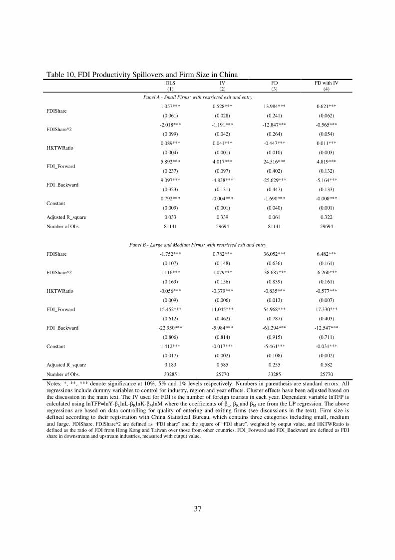
37

Table 10, FDI Productivity Spillovers and Firm Size in China

OLS (1)

IV (2)

FD (3)

FD with IV (4)

Panel A - Small Firms: with restricted exit and entry

1.057*** 0.528*** 13.984*** 0.621*** FDIShare

(0.061) (0.028) (0.241) (0.062)

-2.018*** -1.191*** -12.847*** -0.565*** FDIShare^2

(0.099) (0.042) (0.264) (0.054)

0.089*** 0.041*** -0.447*** 0.011*** HKTWRatio

(0.004) (0.001) (0.010) (0.003)

5.892*** 4.017*** 24.516*** 4.819*** FDI_Forward

(0.237) (0.097) (0.402) (0.132)

9.097*** -4.838*** -25.629*** -5.164*** FDI_Backward

(0.323) (0.131) (0.447) (0.133)

0.792*** -0.004*** -1.690*** -0.008*** Constant

(0.009) (0.001) (0.040) (0.001)

Adjusted R_square 0.033 0.339 0.061 0.322

Number of Obs. 81141 59694 81141 59694

Panel B - Large and Medium Firms: with restricted exit and entry

FDIShare -1.752*** 0.782*** 36.052*** 6.482***

(0.107) (0.148) (0.636) (0.161)

FDIShare^2 1.116*** 1.079*** -38.687*** -6.260***

(0.169) (0.156) (0.839) (0.161)

HKTWRatio -0.056*** -0.379*** -0.835*** -0.577***

(0.009) (0.006) (0.013) (0.007)

FDI_Forward 15.452*** 11.045*** 54.968*** 17.330***

(0.612) (0.462) (0.787) (0.403)

FDI_Backward -22.950*** -5.984*** -61.294*** -12.547***

(0.806) (0.814) (0.915) (0.711)

Constant 1.412*** -0.017*** -5.464*** -0.031***

(0.017) (0.002) (0.108) (0.002)

Adjusted R_square 0.183 0.585 0.255 0.582

Number of Obs. 33285 25770 33285 25770

Notes: *, **, *** denote significance at 10%, 5% and 1% levels respectively. Numbers in parenthesis are standard errors. All regressions include dummy variables to control for industry, region and year effects. Cluster effects have been adjusted based on the discussion in the main text. The IV used for FDI is the number of foreign tourists in each year. Dependent variable lnTFP is calculated using lnTFP=lnY-βLlnL-βKlnK-βMlnM where the coefficients of βL, βK and βM are from the LP regression. The above regressions are based on data controlling for quality of entering and exiting firms (see discussions in the text). Firm size is defined according to their registration with China Statistical Bureau, which contains three categories including small, medium and large. FDIShare, FDIShare^2 are defined as “FDI share” and the square of “FDI share”, weighted by output value, and HKTWRatio is defined as the ratio of FDI from Hong Kong and Taiwan over those from other countries. FDI_Forward and FDI_Backward are defined as FDI share in downstream and upstream industries, measured with output value.

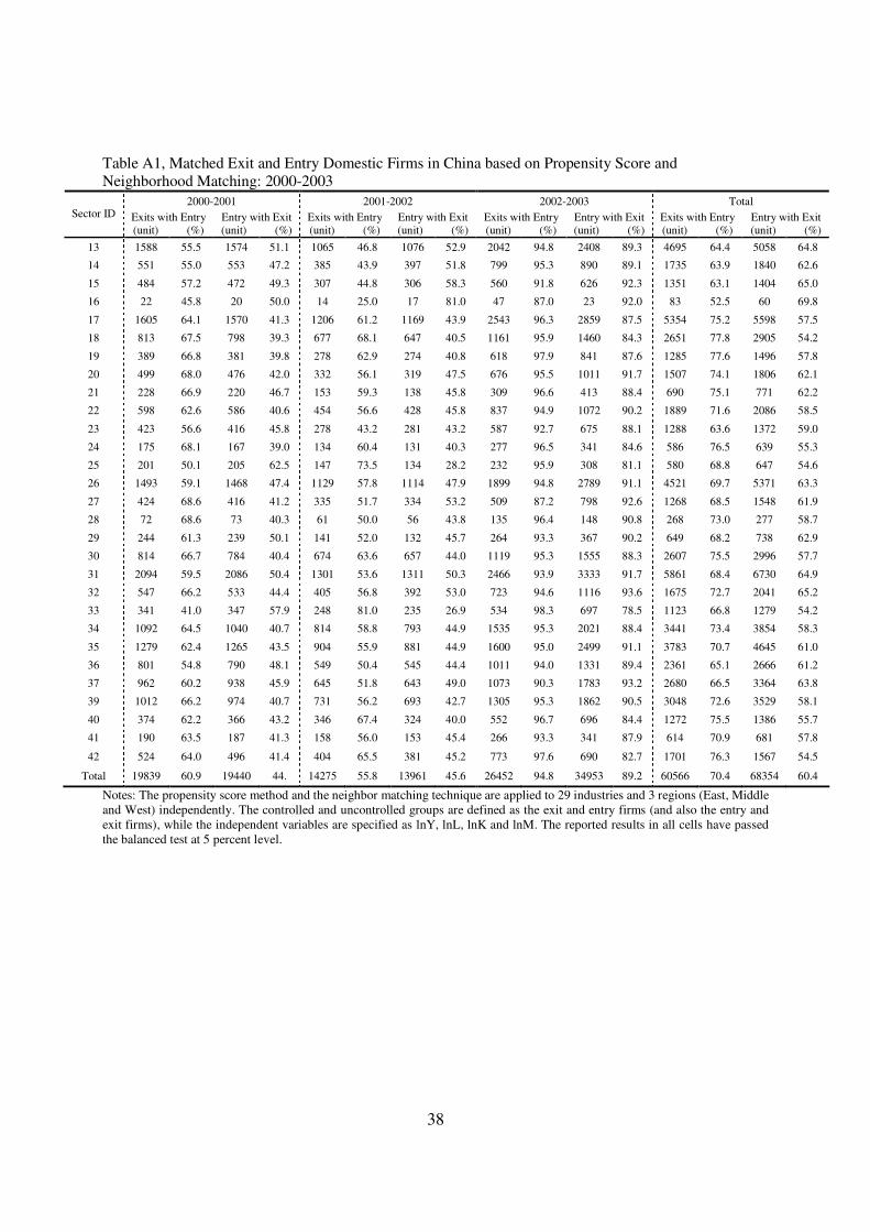
38

Table A1, Matched Exit and Entry Domestic Firms in China based on Propensity Score and Neighborhood Matching: 2000-2003

2000-2001 2001-2002 2002-2003 Total Sector ID Exits with Entry

(unit) (%) Entry with Exit (unit) (%)

Exits with Entry (unit) (%)

Entry with Exit (unit) (%)

Exits with Entry (unit) (%)

Entry with Exit (unit) (%)

Exits with Entry (unit) (%)

Entry with Exit (unit) (%)

13 1588 55.5 1574 51.1 1065 46.8 1076 52.9 2042 94.8 2408 89.3 4695 64.4 5058 64.8

14 551 55.0 553 47.2 385 43.9 397 51.8 799 95.3 890 89.1 1735 63.9 1840 62.6

15 484 57.2 472 49.3 307 44.8 306 58.3 560 91.8 626 92.3 1351 63.1 1404 65.0

16 22 45.8 20 50.0 14 25.0 17 81.0 47 87.0 23 92.0 83 52.5 60 69.8

17 1605 64.1 1570 41.3 1206 61.2 1169 43.9 2543 96.3 2859 87.5 5354 75.2 5598 57.5

18 813 67.5 798 39.3 677 68.1 647 40.5 1161 95.9 1460 84.3 2651 77.8 2905 54.2

19 389 66.8 381 39.8 278 62.9 274 40.8 618 97.9 841 87.6 1285 77.6 1496 57.8

20 499 68.0 476 42.0 332 56.1 319 47.5 676 95.5 1011 91.7 1507 74.1 1806 62.1

21 228 66.9 220 46.7 153 59.3 138 45.8 309 96.6 413 88.4 690 75.1 771 62.2

22 598 62.6 586 40.6 454 56.6 428 45.8 837 94.9 1072 90.2 1889 71.6 2086 58.5

23 423 56.6 416 45.8 278 43.2 281 43.2 587 92.7 675 88.1 1288 63.6 1372 59.0

24 175 68.1 167 39.0 134 60.4 131 40.3 277 96.5 341 84.6 586 76.5 639 55.3

25 201 50.1 205 62.5 147 73.5 134 28.2 232 95.9 308 81.1 580 68.8 647 54.6

26 1493 59.1 1468 47.4 1129 57.8 1114 47.9 1899 94.8 2789 91.1 4521 69.7 5371 63.3

27 424 68.6 416 41.2 335 51.7 334 53.2 509 87.2 798 92.6 1268 68.5 1548 61.9

28 72 68.6 73 40.3 61 50.0 56 43.8 135 96.4 148 90.8 268 73.0 277 58.7

29 244 61.3 239 50.1 141 52.0 132 45.7 264 93.3 367 90.2 649 68.2 738 62.9

30 814 66.7 784 40.4 674 63.6 657 44.0 1119 95.3 1555 88.3 2607 75.5 2996 57.7

31 2094 59.5 2086 50.4 1301 53.6 1311 50.3 2466 93.9 3333 91.7 5861 68.4 6730 64.9

32 547 66.2 533 44.4 405 56.8 392 53.0 723 94.6 1116 93.6 1675 72.7 2041 65.2

33 341 41.0 347 57.9 248 81.0 235 26.9 534 98.3 697 78.5 1123 66.8 1279 54.2

34 1092 64.5 1040 40.7 814 58.8 793 44.9 1535 95.3 2021 88.4 3441 73.4 3854 58.3

35 1279 62.4 1265 43.5 904 55.9 881 44.9 1600 95.0 2499 91.1 3783 70.7 4645 61.0

36 801 54.8 790 48.1 549 50.4 545 44.4 1011 94.0 1331 89.4 2361 65.1 2666 61.2

37 962 60.2 938 45.9 645 51.8 643 49.0 1073 90.3 1783 93.2 2680 66.5 3364 63.8

39 1012 66.2 974 40.7 731 56.2 693 42.7 1305 95.3 1862 90.5 3048 72.6 3529 58.1

40 374 62.2 366 43.2 346 67.4 324 40.0 552 96.7 696 84.4 1272 75.5 1386 55.7

41 190 63.5 187 41.3 158 56.0 153 45.4 266 93.3 341 87.9 614 70.9 681 57.8

42 524 64.0 496 41.4 404 65.5 381 45.2 773 97.6 690 82.7 1701 76.3 1567 54.5

Total 19839 60.9 19440 44. 14275 55.8 13961 45.6 26452 94.8 34953 89.2 60566 70.4 68354 60.4

Notes: The propensity score method and the neighbor matching technique are applied to 29 industries and 3 regions (East, Middle and West) independently. The controlled and uncontrolled groups are defined as the exit and entry firms (and also the entry and exit firms), while the independent variables are specified as lnY, lnL, lnK and lnM. The reported results in all cells have passed the balanced test at 5 percent level.

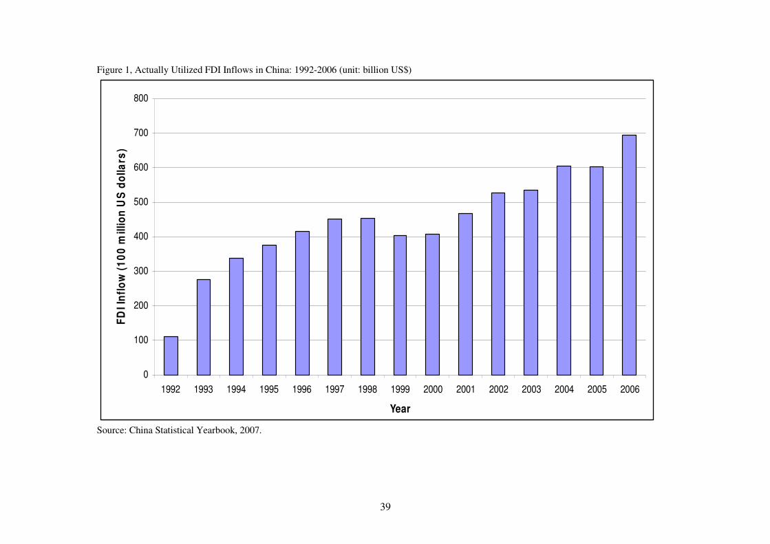
39

Figure 1, Actually Utilized FDI Inflows in China: 1992-2006 (unit: billion US$)

0

100

200

300

400

500

600

700

800

1992 1993 1994 1995 1996 1997 1998 1999 2000 2001 2002 2003 2004 2005 2006

Year

FD

I In

flo

w (

10

0 m

illi

on

US

do

lla

rs)

Source: China Statistical Yearbook, 2007.

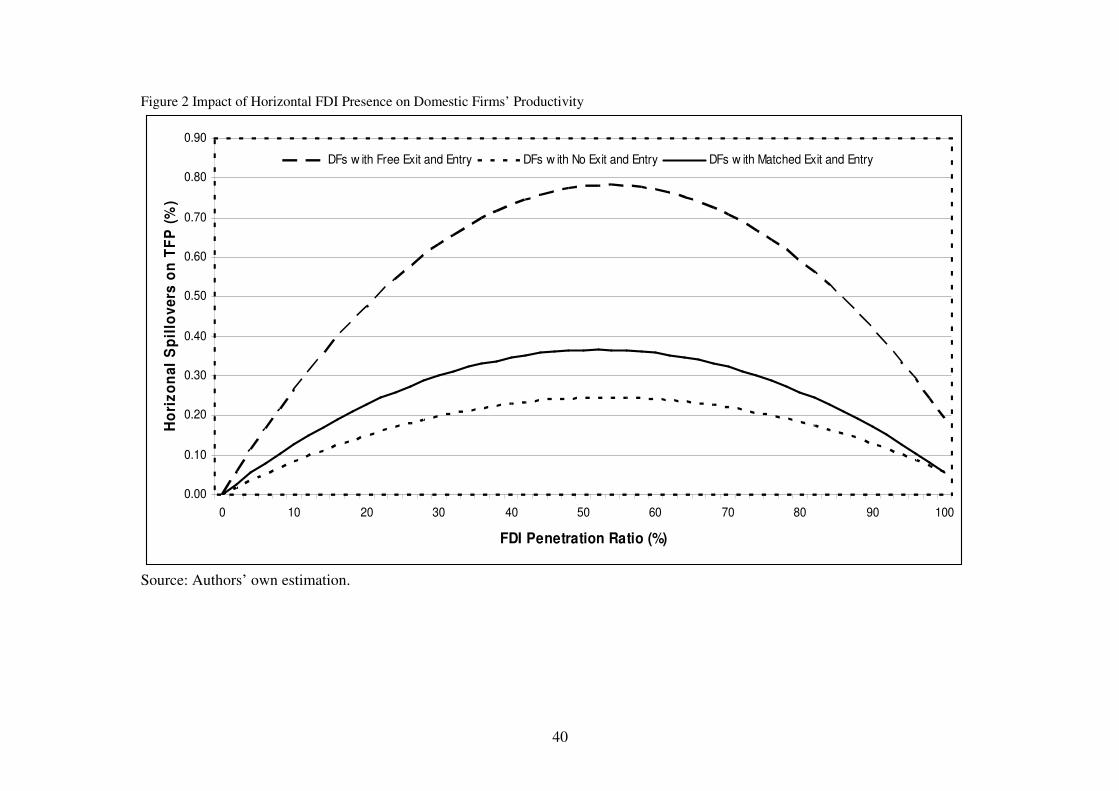
40

Figure 2 Impact of Horizontal FDI Presence on Domestic Firms’ Productivity

0.00

0.10

0.20

0.30

0.40

0.50

0.60

0.70

0.80

0.90

0 10 20 30 40 50 60 70 80 90 100

FDI Penetration Ratio (%)

Ho

riz

on

al

Sp

illo

ve

rs o

n T

FP

(%

)DFs w ith Free Exit and Entry DFs w ith No Exit and Entry DFs w ith Matched Exit and Entry

Source: Authors’ own estimation.

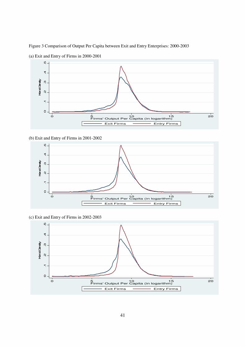
41

Figure 3 Comparison of Output Per Capita between Exit and Entry Enterprises: 2000-2003 (a) Exit and Entry of Firms in 2000-2001

0.1

.2.3

.4.5

Kernal Density

0 5 10 15 20Firms' Output Per Capita (in logarithm)

Exit Firms Entry Firms

(b) Exit and Entry of Firms in 2001-2002

0.1

.2.3

.4.5

Kernal Density

0 5 10 15 20Firms' Output Per Capita (in logarithm)

Exit Firms Entry Firms

(c) Exit and Entry of Firms in 2002-2003

0.1

.2.3

.4.5

Kernal Density

0 5 10 15 20Firms' Output Per Capita (in logarithm)

Exit Firms Entry Firms