Embed Size (px)
Citation preview
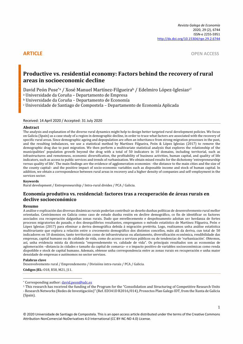
Revista Galega de Economía 2020, 29 (2), 6744 ISSN-e 2255-5951
http://dx.doi.org/10.15304/rge.29.2.6744
1
© 2020 Universidade de Santiago de Compostela. This is an open access article distributed under the terms of the Creative Commons Attribution-NonComercial-NoDerivatives 4.0 International (CC BY-NC-ND 4.0) License.
ARTICLE OPEN ACCESS
Productive vs. residential economy: Factors behind the recovery of rural areas in socioeconomic decline
David Peón Pose*a / Xosé Manuel Martínez-Filgueirab / Edelmiro López-Iglesiasc1 a Universidade da Coruña – Departamento de Empresa b Universidade da Coruña – Departamento de Economía c Universidade de Santiago de Compostela – Departamento de Economía Aplicada Received: 14 April 2020 / Accepted: 31 July 2020
Abstract The analysis and explanation of the diverse rural dynamics might help to design better targeted rural development policies. We focus on Galicia (Spain) as a case study of a region in demographic decline, in order to trace what factors are associated with the recovery of specific rural areas. Since demographic ageing and depopulation are often an inheritance from strong migration processes in the past, and the resulting imbalances, we use a statistical method by Martínez Filgueira, Peón & López Iglesias (2017) to remove the demographic drag due to past migration. We then perform a multivariate statistical analysis that explores the relationship of the municipalities’ population growth beyond the drag with a total of 50 indicators in 10 domains, including territorial, such as infrastructures and remoteness, economic diversification, the profitability of business activities, human capital, and quality of life indicators, such as access to public services and trends of rurbanisation. We obtain mixed results for the dichotomy ‘entrepreneurship versus quality of life’. The main findings are the evidence of agglomeration economies –the distance to the main cities and the size of the county capital– and the positive impact of socio-economic variables such as disposable income and stock of human capital. In addition, we obtain a correspondence between rural areas in recovery and a higher density of companies and self-employment in the services sector.
Keywords Rural development / Entrepreneurship / Intra-rural divides / PCA / Galicia.
Economía produtiva vs. residencial: factores tras a recuperación de áreas rurais en declive socioeconómico
Resumo A análise e explicación das diversas dinámicas rurais poderían contribuír ao deseño dunhas políticas de desenvolvemento rural mellor orientadas. Centrámonos en Galicia como caso de estudo dunha rexión en declive demográfico, co fin de identificar os factores asociados coa recuperación dalgunhas zonas rurais. Dado que envellecemento e despoboamento adoitan ser herdanza de fortes procesos migratorios do pasado, e dos desequilibrios resultantes, empregamos o método estatístico de Martínez Filgueira, Peón e López Iglesias (2017) para eliminar a deriva demográfica debida á migración pretérita. Logo, realizamos unha análise estatística multivariante que explora a relación entre o crecemento demográfico dos distintos concellos, máis alá da deriva, cun total de 50 indicadores en 10 dominios, tanto territoriais como de infraestruturas ou afastamento, diversificación económica, rendibilidade das empresas, capital humano ou de calidade de vida, como do acceso a servizos públicos ou de tendencias de ‘rurbanización’. Obtemos, así, unha evidencia mixta da dicotomía “emprendemento vs. calidade de vida”. Os principais resultados son as economías de aglomeración –distancia ás cidades e tamaño da capital de comarca– e o impacto positivo de variables socioeconómicas como renda dispoñible e stock de capital humano. Ademais, obtense unha correspondencia entre as zonas rurais en recuperación e unha maior densidade de empresas e autónomos no sector servizos.
Palabras clave Desenvolvemento rural / Emprendemento / Divisións intra-rurais / PCA / Galicia.
Códigos JEL: O18, R58, M21, J11.
* Corresponding author: [email protected] 1 This research has received the funding of the Program for the “Consolidation and Structuring of Competitive Research Units - Research Networks (Redes de Investigación)" (Ref. ED341D R2016/014), Proxectos Plan Galego IDT, from the Xunta de Galicia (Spain).
Peón, D., Martínez-Filgueira, X. M., & López-Iglesias, E. Revista Galega de Economía 2020, 29 (2), 6744
2
1. Introduction
Many rural areas in Europe continue to exhibit a significant lag in terms of economic development and social well-being (Akgün, Baycan & Nijkamp, 2015; Spoor, 2013), having an impact on their population structure and dynamics (European Commission, 2013). The design of effective public policies to promote social and territorial development and cohesion must be based on an analysis of the factors that lie behind successful experiences. In this respect, it is convenient to replace the traditional urban-rural dichotomy by the analysis of intra-rural divides (Rizzo, 2016): the interpretation of the diverse rural dynamics, with some rural areas performing much better than others and, in some cases, even better than urban areas (Bryden & Munro, 2000), might be helpful for the design of rural development policies.
In the analysis of factors behind intra-rural divides, researchers recurrently consider geographical and territorial dimensions (Salvati & Carluci, 2016; Smailes, Argent & Griffin, 2002), rurbanisation (Eliasson, Westlund & Johansson, 2015), employment and economic diversification (e.g., Marsden & Sonnino, 2008), amenities and agritourism (Figueiredo, 2009; Phelan & Sharpley, 2011), entrepreneurship and business growth (Li, Goetza, Partridge & Fleming, 2016; Stephens, Partridge & Faggian, 2013), and access to public services and better institutional governance (Sánchez-Zamora, Gallardo-Cobos & Ceña-Delgado, 2014). These are summarized in the classic dichotomy of what should come first: fostering business activities and entrepreneurship in areas where socioeconomic indicators are weak, versus ensuring higher quality of life standards for residents in rural areas. The first option considers two directions (Barbut, 2009): the “productive economy”, with the logic of boosting the competitiveness of the local economy in order to sell goods and services outside the rural territory, and the “residential economy”, which sells them locally instead, seeking to create local jobs attracting residents, tourists and retirees (Bureau, 2016). Alternatively, the quality-of-life strategy works in the same direction as the residential economy, providing residents and visitors with access to public services and facilities of standards similar to those in urban areas.
We aim to contribute to this literature with a case study, Galicia (Spain), a paradigmatic example of an aged region in demographic decline, resulting from an unbalanced demographic structure inherited from strong migration processes since the 19th century and especially during the period 1950-1975. The case study might easily apply to other regions with a similar background: history may represent a heavy burden, particularly in rural areas, when they experienced large migration processes in the past. The consequences of population decline are often self-reinforcing, bringing about more population decline (Elshof, van Wissen & Mulder, 2014).
Thus, the first part of our research is devoted to identify and remove the negative effect from past migration, following Martínez Filgueira et al. (2017) methodology. We apply that statistical treatment to all the 315 Galician municipalities to estimate the residuals of their demographic drag. Positive residuals identify municipalities that, despite possibly losing more population in the last two decades (1991-2011), exhibit, at least, a partial, true recovery, as they are being able to moderate or even reverse the depopulation process inherited from the past.
Then, in the second part of our research, we focus on the 264 municipalities in Galicia that are classified as rural according to DEGURBA standards (Instituto Galego de Estatística [IGE], 2011), to perform a principal component analysis (PCA) on a series of dimensions, including business performance and quality of life indicators, among others. By obtaining the factors that are related to population performance, measured through the residuals beyond the drag, we trace the dimensions that better explain the ability of rural areas to overcome the processes of ageing and depopulation. We obtain relevant results in two realms: territorial (the distance to the main urban areas and the population of the county capital) and socio-economic conditions (the ratio of university graduates and tdisposable income). Finally, a correspondence between rural areas in recovery and a higher density of companies and self-employment in the services sector is also observed.
The structure of the article is as follows. In Section 2, we analyse the depopulation process observed in the rural areas of Galicia, and obtain, for the period 1991-2011, the residuals of the demographic drag
Peón, D., Martínez-Filgueira, X. M., & López-Iglesias, E. Revista Galega de Economía 2020, 29 (2), 6744
3
inherited from past migration processes at municipal level. Section 3 provides a multivariate statistical analysis devoted to interpret the factors that would explain the recovery of some rural areas verified in the previous data. Finally, Section 4 concludes. Additional information regarding methodology and econometric results may be found in the Supplementary Material (SM).
2. The depopulation process of rural areas in Galicia in the recent decades and the residuals of the demographic drag
2.1. Recent demographic dynamics in Galicia (1991-2011)
Galicia, in the North-West of the Iberian Peninsula, is a NUTS 2 region and one of the seventeen Autonomous Communities in Spain, with an extension similar to that of Belgium (about 30,000 square kilometres)with a population of 2.75 million inhabitants. It has historically lagged Spain in terms of population and GDP growth, persistently losing relative weight. The GDP per capita by 2014 was 80% of the EU-28 average in PPS terms, down from 92.3% in 2009 (Xunta de Galicia, 2014).
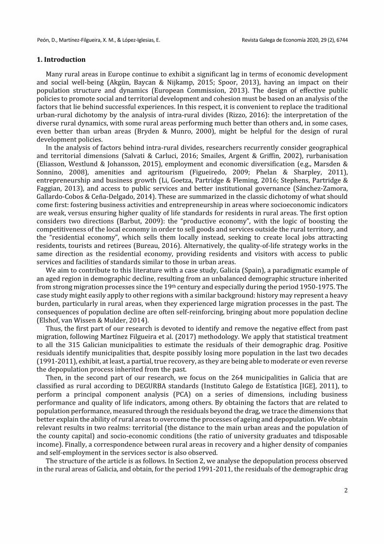
What makes Galicia an interesting case study is that it represents a region in demographic decline. The average age of the population is four years higher than that of Spaniards and Europeans, and the fertility rate is among the lowest in the world (1.07 children per woman), contributing to a strongly negative vegetative balance (-3.03 per thousand). Projections estimate that Galicia might lose a million inhabitants by 2050 (Xunta de Galicia, 2013). The dynamics of rural areas is even worse. Since the mid-twentieth century, Galicia experienced a late and abrupt agricultural sector decline, reducing its share in total employment from 70% to less than 5%. This intense sectoral restructuring resulted in a reduction of total employment, leading, at the same time , to strong rural-urban migration flows within the region (López Iglesias, 1995). Today, almost 70% of the population lives in 15% of the territory, a line in the West known as the Eixo Atlántico that goes from the North to the Portuguese border in the South and includes the largest cities of A Coruña and Vigo (about 300,000 inhabitants each) and the administrative capital, Santiago de Compostela – see Figure 1.
Figure 1. Territorial distribution of the Galician population. Density by municipalities 2011 and urban-rural typology (DEGURBA). Source: Own elaboration. Data: Instituto Nacional de Estadística (INE), Census 2011; IGE (2011).
As a result of past migration flows, rural areas inherited an unbalanced demographic structure that has conditioned their dynamics in recent decades. Figure 2 shows the population change of
Peón, D., Martínez-Filgueira, X. M., & López-Iglesias, E. Revista Galega de Economía 2020, 29 (2), 6744
4
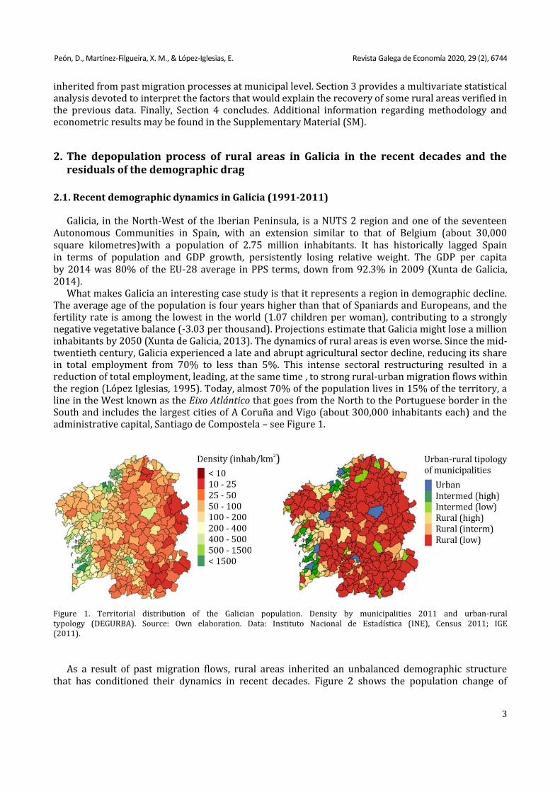
each municipality from 1991 to 2011 –which we denote DEPOP91-11. The demographic dynamics continue to favour the concentration of the Galician population in the West, with the exceptions being the Northern coastal area, the two inner capitals of province –Lugo and Ourense– and a few villages of intermediate size. We may see the inner Galicia experiencing a strong depopulation process, with the most severe examples often related to municipalities in the mountains –to the East and South. This performance is difficult to reverse, as it is not caused by continued negative migration flows, but by the negative vegetative balance due to a demographic burden that is the consequence of past migrations (López Iglesias, 2013). We analyse this negative effect next.
Figure 2. Population change of Galician municipalities. Years 1950-1991 (EMIG50-91) and 1991-2011 (DEPOP91-11). Source: Own elaboration. Data: INE, Census 1950, 1991, 2011.
Based on these initial findings, we follow Martínez Filgueira et al. (2017) methodology to set this hypothesis: the depopulation of rural municipalities in recent decades is due, to a large extent, to the demographic structure in early 1990s and this, in turn, is a consequence of past migration during the period 1950-1991. Thus, for changes in population, we retain three key dates: 1950, 1991 and 20112. The first one represents the beginning of the last historical migration period in Galicia that started in the 1950s and stopped after the 1970s crisis due to a sudden cut in the number of migrants to Europe. However, part of that migration does not appear in the official statistics until the 1991 Census –reflected in a significant net migration officially recorded in the 1981-1991 decade (Fernández Leiceaga & López Iglesias, 2000). Finally, we use 2011 since this represents the last Census available.
Consequently, we define the variable EMIG50-91 as the annualized percentage of population change between 1950 and 1991, a proxy of the strong emigration in these four decades and, particularly, in the 1950-1975 period. We may appreciate a widespread population decline, where three quarters of the Galician territory saw its human potential diminished –see Figure 2. A dual pattern was developed: municipalities with a population density above 200 inhab/km2 by 1950 increased or hardly lost population, while only a few exceptions below 150 inhab/km2 could prevent population loss.
2 Any changes in the municipality map of Galicia since 1950 were taken into account (see Míguez Macho, 2013 for a review). See the SM for a detailed description of sources and relevant details in data processing.
Peón, D., Martínez-Filgueira, X. M., & López-Iglesias, E. Revista Galega de Economía 2020, 29 (2), 6744
5
2.2. The residuals of the demographic drag (1991-2011)
We firstly demonstrate the decisive role of the migration flows occurring from 1950 to 1991 as determinant of the demographic structure of the municipalities in 1991. Consequently, we then use it to obtain the residuals of the demographic drag (the population dynamics in the period 1991-2011 after discounting the dragging effect from the past).
Step 1. Historic migration, reflected in the population change 1950-1991 (EMIG50-91), as a determinant of the demographic structure of municipalities in 1991.
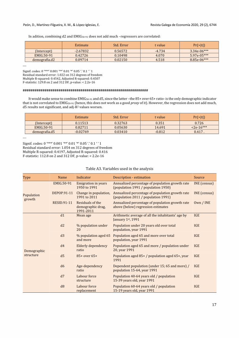
We test the hypothesis that the variable EMIG50-91 explains the differences in the demographic structure of the Galician municipalities in 1991, and, particularly, the heavily skewed structure we find (to different degrees) in rural municipalities. We analyse the correlation of EMIG50-91 with the demographic variables mean age (d1), the percentage of population under 20 (d2), the percentage of population over 65 (d3), the elderly dependency ratio (d4), the 85+ over 65+ ratio (d5), the age-dependency ratio (d6), the labour force structure (d7) and the labour force replacement (d8). Results are provided in Table A1 in the SM.
Overall, the results confirm the hypothesis: correlations of 75% to 90%, significantly different from zero, and signs of consistent interpretation. The only exception is a correlation coefficient of -0.16 with variable d5 (the percentage of population 85 years old or more to the group of 65 or more), which makes sense, since this ratio would be a consequence of demographic phenomena before 1950. Higher correlation levels are observed with age structure (d1 and d3 with -0.89, and d2 with +0.86). Then, with correlation coefficients higher than 0.80, indicators that reflect the aging of population (d4 and d8), and with coefficients above 0.75 those of the structure of active population (d6 and d7). These results support using EMIG50-91 as a synthetic indicator or proxy of the demographic drag effect –i.e. the inertia of past population dynamics. However, we must see whether it is more appropriate to use EMIG50-91 or any of the indicators of the demographic structure in 1991. We carry out this analysis in the next step.
Step 2. Testing the validity of EMIG50-91 as the best proxy of demographic drag
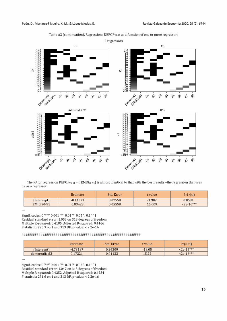
We follow Martínez Filgueira et al. (2017) to first observe, in Table A1, that the correlation between EMIG50-91 and DEPOP91-11 is strong as well, close to 65%, significant and of consistent interpretation. The validity of EMIG50-91 as a proxy of the demographic drag is then tested through the goodness of fit for different regressions on DEPOP91-11. We perform a selection of variables for the regression DEPOP91-11 to EMIG50-91 and the demographic variables d1 to d8, indicators of the demographic structure in 1991. As selection criteria we use BIC and Mallows Cp for regressions with one or two regressors, taking the explanatory power of the model in consideration – see Table A2 in the SM.
We find DEPOP91-11 = f (EMIG50-91) is the regression that best fits the recent population trends, together with the regressions that include d2 and d3 (percentage of younger than 20 and older than 65). The goodness of fit of regression DEPOP91-11 = f (EMIG50-91) is almost identical in terms of R2 to the regression with best results – the one that uses d2 as a regressor – but introducing EMIG50-91 and d2 together does not add much. It would perhaps make sense to use EMIG50-91 and d5, since these two variables are not correlated. However, the regression barely gives additional information, d5 appears to be non-significant, and the adj-R2 worsens.
Step 3. The population performance beyond the demographic drag
The significant correlation between EMIG50-91 and DEPOP91-11 indicates that the population dynamics at the municipal level in the period 1991-2011 are strongly affected by the migration flows in the

Peón, D., Martínez-Filgueira, X. M., & López-Iglesias, E. Revista Galega de Economía 2020, 29 (2), 6744
6
previous decades. However, the value (0.65) of the correlation coefficient, far from one, indicates relevant variations across municipalities with regard to previous trends, and is lower than the correlation at the county level, 0.83 (Martínez Filgueira et al., 2017) –which indicates that Galician counties hide relevant differences in the behaviour of the municipalities within3.
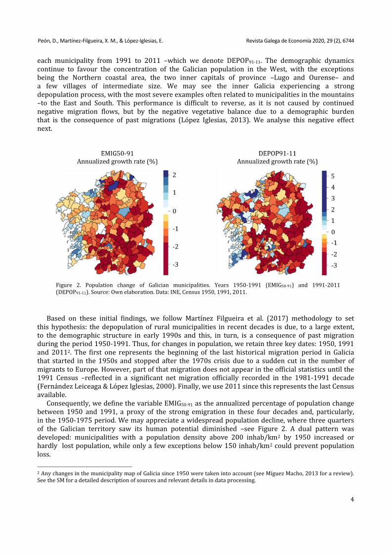
Hence, we move on to identify to what extent the dynamics exhibit new developments with regard to previous trends. This is what the analysis of the regression residuals allows us to do. We define variable RESID91-11 as the residuals of the regression DEPOP91-11 = f (EMIG50-91). They provide the demographic performance of the Galician municipalities once the drift from past migrations is discounted. Figure 3 shows the residuals RESID91-11.
Figure 3. Residuals of the demographic drag by municipalities. Source: Own elaboration.
Figure 3 provides an alternative view of the population dynamics in Galicia, where the depopulation process not inherited from the past is not widespread. The areas with a better performance, clearly improving their relative dynamics in the last two decades, are primarily concentrated in the vicinity of the cities and along the Eixo Atlántico, as well as in the outskirts of the inner city of Ourense. In addition, we may talk of a central Galicia with stable population levels, once the drift from the past is removed –though with some negative cases, related to orography.
Indeed, negative performance (i.e., an accelerated depopulation beyond the dragging effect from the past) seems to be linked to adverse orography. Thus, much of the Galician municipalities with negative residuals are in the line formed by the mountain ranges of Xistral, Ancares, Courel, Macizo Central, and Trevinca which extends along the Northern and Eastern third of the region. Similar results are observed in the Dorsal Central, another mountainous area that goes from North to South in the centre of Galicia. Finally, we may observe two coastal areas with bad performance. The first one to the North –corresponding to the municipalities of Ferrol, Fene, As Pontes and Ortigueira –is the result of the restructuring of the shipping industry located there in the 1980s. The second one, and the worst case in terms of relative decline compared to previous trends, is a coastal area to the West of the Eixo Atlántico, known as the Costa da Morte. This is a rural area where the decline would correspond to late employment reductions in agrarian and fishery sectors.
3 The 315 municipalities of Galicia are grouped in 53 counties (“comarcas”), a unit officially recognized of closely related municipalities, but without administrative effects.

Peón, D., Martínez-Filgueira, X. M., & López-Iglesias, E. Revista Galega de Economía 2020, 29 (2), 6744
7
3. The factors behind the recovery of rural areas in socioeconomic decline
We seek to investigate several interconnected causes analysed without hierarchical causality, trying to capture the complexity of processes and aspects that influence the dynamics of rural areas, in a way that linear and hierarchical approaches should be avoided (Salvati & Carlucci, 2016). We focus on the rural municipalities, according to the characterization by the Galician Statistics Institute (IGE) following DEGURBA standards (Eurostat, 2011) –recall Figure 1 above–4. We trace which factors, and particularly those related to business activities and quality of life, are associated with the recovery or improvement of rural areas.
3.1. Variables and data
Most variables come from data provided by official statistical sources –the Spanish Statistics Institute (INE) and the IGE, as well as some agencies from the Spanish and Galician ministries–, while business financial data was obtained from SABI –Bureau van Dijk database. The area under study is the whole population of 315 Galician municipalities up to 2011, of which the 264 classified as rural, according to IGE, are the main research target. The period considered is from 1991 to 2011, to observe, in particular, how the socio-economic situation of the municipalities in early 1990s implies a path dependence on their population growth throughout the two decades under analysis. We will add some insights on the dichotomy ‘entrepreneurship vs. quality of life’. Here, due to lack of data available, we will observe the consequences at period end (year 2011) of a positive demographic performance. Hence, any causal interpretation of the impact of entrepreneurship or quality of life factors should be avoided. However, this analysis might offer some insights on the ability of municipalities to reverse path dependence.
The variables were classified within 10 domains, for a total of 50 indicators. Table A3 in the SM provides all indicators, including their description or estimation procedure, and data sources. The first domain includes the population growth variables DEPOP91-11 and RESID91-11, the interpretation of which is the main object of study. These, together with EMIG50-91 (now excluded in this analysis) and the indicators in the second domain –demographic structure– were already described in Section 2. To them we add a series of socio-economic domains that might be potential sources of population growth for rural areas beyond their demographic drag. These include territorial variables such as infrastructures and remoteness (e.g., Smailes et al., 2002), the stock of human capital, including education and labour market (Salvati and Carlucci, 2016), economic diversification (e.g., Marsden & Sonnino, 2008), tprofitability and shifts in the location of business activities (Stephens et al., 2013), and quality of life indicators –including personal income, access to public services (Sánchez-Zamora et al., 2014) and amenities (Figueiredo, 2009), and trends of urban lifestyles in rural areas (Eliasson et al., 2015).
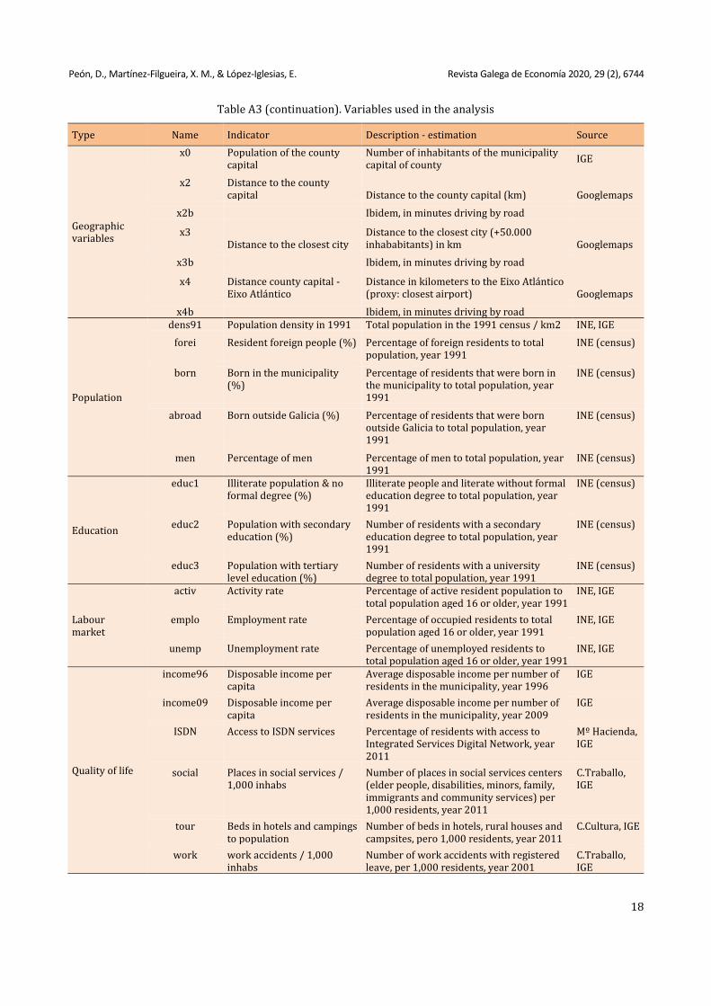
In what follows, we summarize the indicators we used for these eight additional domains. Thus, geographical and population variables are included in four domains. First, for each municipality, we consider geographical variables such as the population of the county capital in year 1991 (x0) and its natural logarithm (log_x0), the distances in kilometres to the county capital (x2), to the closest city (x3) and to the Eixo Atlántico (x4), as well as those distances in minutes by road (x2b, x3b and x4b, respectively). These data consider Galicia an island:, the effects that other growth poles in North Portugal and the rest of Spain could have on Galician border areas are not observed. Second, to approach the characteristics of each municipality’s population up to 1991 we take the population density (dens91), percentage of foreign residents (forei), percentage of residents that were born in the municipality (born), percentage of residents that were born outside Galicia (abroad) –these two as a
4 The IGE recently provided an updated classification (IGE, 2016) using the same methodology. The number of rural municipalities would now be reduced to 240, of which only two were considered to be intermediate in 2011.
Peón, D., Martínez-Filgueira, X. M., & López-Iglesias, E. Revista Galega de Economía 2020, 29 (2), 6744
8
proxy for the ability of each municipality to attract people from other territories– and the percentage of men (men) to total population. Third, we consider three indicators for the education level up up 1991: namely, the percentage of illiterate population or literate with no formal degree (e1), the percentage of population with secondary education (e2) and with tertiary level education (e3) and fourth, three indicators of the labour market, namely, the activity rate (active), employment rate (emplo) and unemployment rate (unemp).
A seventh domain seeks to include some quality of life indicators. We had to use a variety of indeces in different instances, but we still had problems obtaining statistics that are either available for all municipalities, referring to the period of study, and representative of such instances. For personal income we use the disposable income per capita (income96) in 1996 (the oldest data available), representative of the structural conditions of each municipality at the beginning of the period of analysis. For other indicators we had to use a series of proxies, all of them referring to the end of the period (2011). The percentage of residents with access to integrated services digital network (ISDN) is used as a proxy of trends in urban lifestyles as well as for access to public services, the latter together with the number of places in social services centres for older people, disabilities, minors, family, immigrants and community services (social). In addition, we use the number of beds in hotels, rural houses and campsites per 1,000 residents (tour) as a proxy for the existence of amenities, and the ratio of work accidents with registered leave per 1,000 inhabitants (work) as an indicator of quality of life at work. Finally, the disposable income per capita (income09) at the end of the period of analysis –2009 , in this case due to lack of official data for 2011– is used again in order to have data consistent with the other proxy indicators for quality of life.
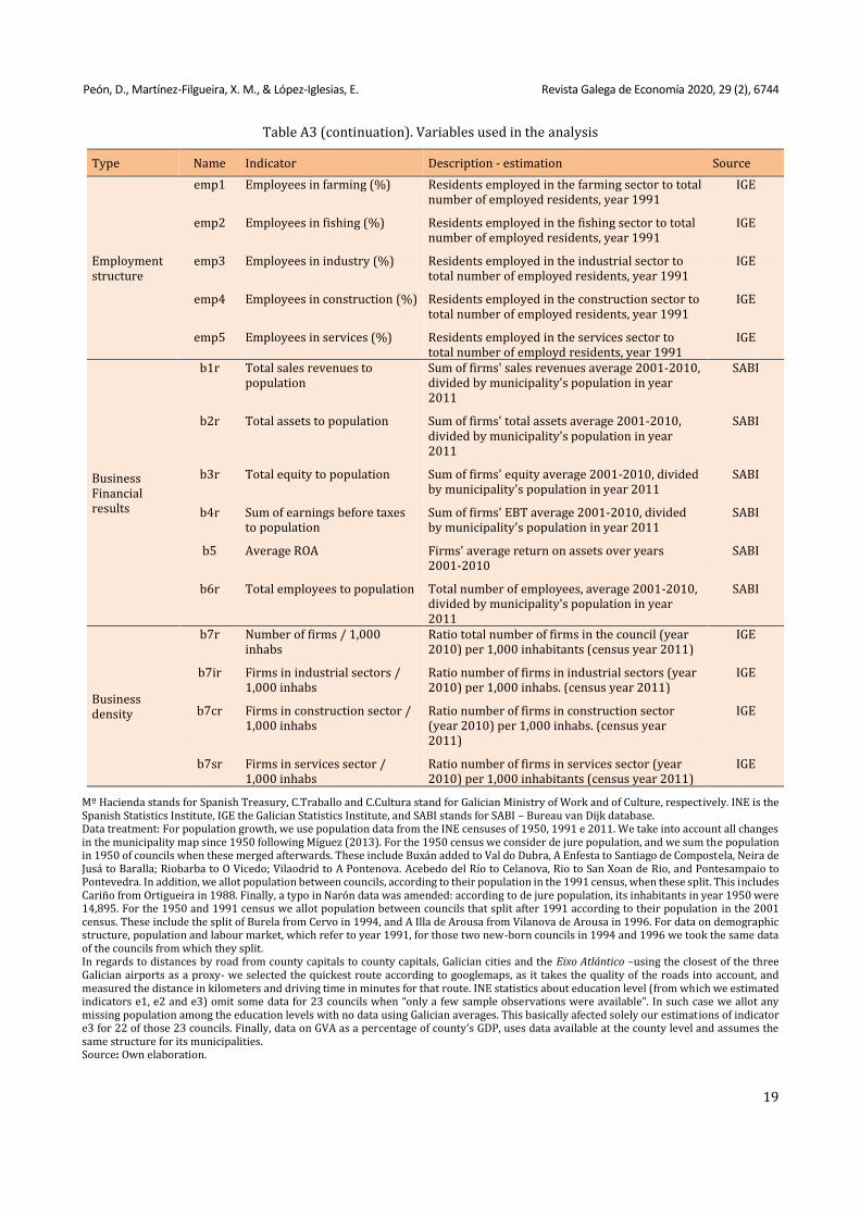
Finally, in terms of economic activity and entrepreneurship we obtained indicators in the three last domains. The first one (the eighth in the overall list) is the sectoral structure of employment in 1991, to be interpreted together with other variables that account for the structural factors of the municipality at the beginning of the period of analysis. This domain includes the percentage of total employment in the following sectors: farming (emp1), fishing (emp2), industry (emp3), construction (emp4), and services (emp5). The two other domains use more recent data for the end of the period of analysis, again, due to lack of data in some instances– trying to capture the dimension and performance of business activities in relation to the population of each municipality. Thus, the ninth domain summarizes the business financial results of any firms in each municipality with complete data in the SABI database over the period 2001-2010. We have considered four ratios –total sales revenues (b1r), total assets (b2r), total equity (b3r), and earnings before taxes (b4r)– that estimate the sum of these accounting measures for all firms divided by the population of the municipality. In addition, we obtained the firms' average return on assets (b5) and the ratio of all the firms’ employees to the municipality’s population (b6r). Since the SABI database provides only a sample of all firms registered in a municipality, we considered a tenth and last domain where we use data from IGE to obtain four indicators of business density. The main contribution made by including these variables is to take into account the role of self-employment5. These are the number of firms per 1,000 inhabitants (b7r), and the equivalent measures for the firms in industrial sector (b7ir), construction (b7cr) and services sector (b7sr) –all of them referring to 2010.
3.2. Descriptive statistics
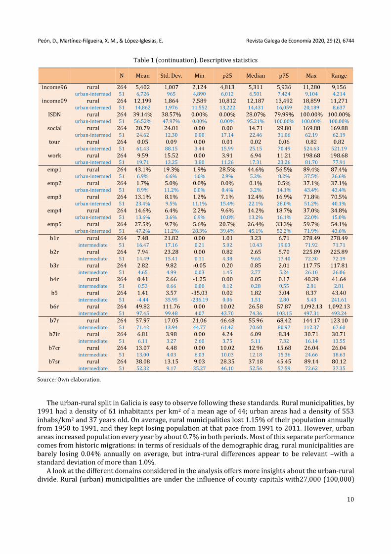
Table 1 provides the main descriptive statistics for the indicators previously explained. For each indicator, the estimations refer to the 264 rural municipalities under study (1.09 million inhabitants in 2011), and they are compared below with the equivalent results for the 51 urban and intermediate municipalities (1.69 million inhabitants in 2011).
5 IGE has more than 120,000 firms registered in rural and intermediate municipalities in year 2011, of which 74,000 are self-employed workers. PLCs, Ltds and cooperatives amount to 37,500 companies, and SABI lists 8,800.

Peón, D., Martínez-Filgueira, X. M., & López-Iglesias, E. Revista Galega de Economía 2020, 29 (2), 6744
9
Table 1. Descriptive statistics
N Mean Std. Dev. Min p25 Median p75 Max Range
EMIG.5091 rural 264 -1.1460% .8454% -3.5982% -1.7538% -1.1673% -.5511% 2.2381% 5.8362% urban-intermed 51 .7343% .6356% -.8743% .2726% .6751% 1.1562% 2.2374% 3.1117%
DEPOP.9111 rural 264 -1.1372% 1.2458% -3.8721% -1.9460% -1.3162% -.4811% 5.4812% 9.3534% urban-intermed 51 .6621% 1.0072% -.9978% .1378% .5148% 1.0858% 3.5477% 4.5455%
RESID.9111 rural 264 -.0374% 1.0455% -3.8514% -.5934% -.0923% .4654% 5.6404% 9.4918% urban-intermed 51 .1936% 1.0735% -2.4330% -.3296% .0712% .5652% 2.6843% 5.1173%
d1 rural 264 43.8 4.1 33.8 40.7 44.6 46.6 53.7 19.9 urban-intermed 51 36.8 2.4 32.9 34.9 36.2 37.9 43.2 10.3
d2 rural 264 21.3 4.6 10.8 18.1 20.5 24.6 33.4 22.7 urban-intermed 51 28.9 3.1 21.1 26.4 29.2 31.4 34.8 13.7
d3 rural 264 23.4 6.0 9.9 18.8 24.4 27.7 38.6 28.7 urban-intermed 51 13.6 2.9 9.4 11.3 12.5 14.9 23.0 13.6
d4 rural 264 121.1 56.8 30.7 76.7 121.8 149.4 351.3 320.5 urban-intermed 51 48.5 16.5 27.2 36.4 43.5 52.4 109.3 82.2
d5 rural 264 9.7 1.8 3.4 8.5 9.6 10.6 15.5 12.0 urban-intermed 51 9.0 1.5 6.5 8.1 8.8 10.0 12.1 5.6
d6 rural 264 62.5 8.6 41.1 56.2 61.1 68.3 90.0 49.0 urban-intermed 51 51.2 3.9 41.7 49.5 50.9 52.5 61.6 19.9
d7 rural 264 104.8 21.4 64.2 88.1 103.7 117.9 183.0 118.8 urban-intermed 51 75.2 9.9 59.3 67.0 72.1 82.9 97.5 38.2
d8 rural 264 120.5 45.1 41.2 84.7 116.4 148.2 300.0 258.8 urban-intermed 51 60.1 15.1 41.4 49.4 57.2 68.2 117.2 75.8
x0 rural 264 26,832 44,999 1,874 7,016 11,134 20,318 276,109 274,235 urban-intermed 51 100,210 105,086 7,109 15,242 32,170 246,953 276,109 269,000
log_x0 rural 264 9.51 1.04 7.54 8.86 9.32 9.92 12.53 4.99 urban-intermed 51 10.85 1.24 8.87 9.63 10.38 12.42 12.53 3.66
x2 rural 264 14.9 9.3 0.0 8.6 14.8 20.9 49.6 49.6 urban-intermed 51 9.5 10.2 0.0 0.0 7.2 18.3 38.9 36.9
x2b rural 264 17.4 10.1 0.0 11.0 17.0 24.0 50.0 50.0 urban-intermed 51 11.2 10.9 0.0 0.0 12.0 19.0 38.0 38.0
x3 rural 264 45.4 25.3 5.1 26.5 40.9 55.6 143.0 137.9 urban-intermed 51 30.3 27.4 0.0 11.3 23.6 42.3 113.0 113.0
x3b rural 264 41.6 19.1 10.0 28.0 37.0 51.0 135.0 125.0 urban-intermed 51 27.8 21.7 0.0 15.0 25.0 36.0 90.0 90.0
x4 rural 264 89.2 49.8 11.2 48.0 80.0 127.0 245.0 233.8 urban-intermed 51 51.8 44.2 4.4 20.4 42.3 71.3 219.0 214.6
x4b rural 264 62.9 29.5 13.0 40.0 60.5 81.8 175.0 162.0 urban-intermed 51 38.5 26.2 7.0 19.0 32.0 51.0 126.0 119.0
dens91 rural 264 61.2 65.4 4.7 26.8 40.7 74.4 692.9 688.2 urban-intermed 51 552.8 941.0 53.5 223.2 366.4 520.9 6567.9 6514.4
forei rural 264 0.69% 1.31% 0.00% 0.17% 0.38% 0.72% 15.41% 15.41% urban-intermed 51 0.70% 0.56% 0.07% 0.37% 0.55% 0.87% 3.37% 3.30%
born rural 264 78.7% 8.6% 38.3% 75.4% 80.0% 84.2% 96.5% 58.2% urban-intermed 51 64.0% 14.4% 30.5% 54.7% 64.1% 75.0% 85.1% 54.5%
abroad rural 264 5.1% 3.7% 0.7% 2.8% 4.2% 6.2% 27.1% 26.5% urban-intermed 51 6.5% 3.5% 1.7% 3.4% 5.6% 8.5% 17.0% 15.3%
men rural 264 48.9% 1.7% 43.9% 48.0% 48.9% 49.8% 55.2% 11.3% urban-intermed 51 48.4% 0.8% 46.9% 48.0% 48.4% 49.0% 50.4% 3.5%
educ1 rural 264 43.5% 13.6% 5.9% 34.8% 44.7% 54.6% 77.1% 71.2% urban-intermed 51 24.7% 7.6% 13.9% 19.5% 23.8% 27.5% 59.8% 46.0%
educ2 rural 264 18.3% 3.7% 8.1% 15.7% 18.1% 20.6% 32.7% 24.6% urban-intermed 51 26.9% 4.1% 18.5% 23.5% 26.5% 29.7% 37.3% 18.8%
educ3 rural 264 2.0% 1.0% 0.1% 1.2% 1.8% 2.3% 7.2% 7.1% urban-intermed 51 4.1% 2.3% 1.4% 2.6% 3.3% 4.7% 12.4% 11.0%
activ rural 264 47.5 7.6 31.1 43.0 46.4 51.2 91.3 60.2 urban-intermed 51 48.1 4.6 38.6 45.2 48.3 51.0 61.2 22.6
emplo rural 264 41.5 8.7 23.0 36.0 40.5 45.4 90.5 67.5 urban-intermed 51 39.2 4.6 28.7 36.9 39.7 42.2 52.6 23.9
unemp rural 264 13.0 6.2 1.0 8.7 12.4 16.6 34.7 33.7 urban-intermed 51 18.7 4.5 9.1 15.8 17.6 21.6 29.7 20.6
Peón, D., Martínez-Filgueira, X. M., & López-Iglesias, E. Revista Galega de Economía 2020, 29 (2), 6744
10
Table 1 (continuation). Descriptive statistics
N Mean Std. Dev. Min p25 Median p75 Max Range
income96 rural 264 5,402 1,007 2,124 4,813 5,311 5,936 11,280 9,156 urban-intermed 51 6,726 965 4,890 6,012 6,501 7,424 9,104 4,214
income09 rural 264 12,199 1,864 7,589 10,812 12,187 13,492 18,859 11,271 urban-intermed 51 14,862 1,976 11,552 13,222 14,431 16,059 20,189 8,637
ISDN rural 264 39.14% 38.57% 0.00% 0.00% 28.07% 79.99% 100.00% 100.00% urban-intermed 51 56.52% 47.97% 0.00% 0.00% 95.21% 100.00% 100.00% 100.00%
social rural 264 20.79 24.01 0.00 0.00 14.71 29.80 169.88 169.88 urban-intermed 51 24.62 12.30 0.00 17.14 22.46 31.06 62.19 62.19
tour rural 264 0.05 0.09 0.00 0.01 0.02 0.06 0.82 0.82 urban-intermed 51 61.43 88.15 3.44 15,99 25.15 70.49 524.63 521.19
work rural 264 9.59 15.52 0.00 3.91 6.94 11.21 198.68 198.68 urban-intermed 51 19.71 13.25 3.80 11.26 17.31 23.26 81.70 77.91
emp1 rural 264 43.1% 19.3% 1.9% 28.5% 44.6% 56.5% 89.4% 87.4% urban-intermed 51 6.9% 6.6% 1.0% 2.9% 5.2% 8.2% 37.5% 36.6%
emp2 rural 264 1.7% 5.0% 0.0% 0.0% 0.1% 0.5% 37.1% 37.1% urban-intermed 51 8.9% 11.2% 0.0% 0.4% 3.2% 14.1% 43.4% 43.4%
emp3 rural 264 13.1% 8.1% 1.2% 7.1% 12.4% 16.9% 71.8% 70.5% urban-intermed 51 23.4% 9.5% 11.1% 15.4% 22.1% 28.0% 51.2% 40.1%
emp4 rural 264 14.6% 6.4% 2.2% 9.6% 14.2% 18.7% 37.0% 34.8% urban-intermed 51 13.6% 3.6% 6.9% 10.8% 13.2% 16.1% 22.0% 15.0%
emp5 rural 264 27.5% 9.7% 5.6% 20.7% 26.4% 33.3% 59.7% 54.1% urban-intermed 51 47.2% 11.2% 28.3% 39.4% 45.1% 52.2% 71.9% 43.6%
b1r rural 264 7.48 21.82 0.00 1.01 3.23 6.71 278.49 278.49 intermediate 51 16.47 17.16 0.21 5.02 10.43 19.03 71.92 71.71
b2r rural 264 7.94 23.28 0.00 0.82 2.65 5.70 225.89 225.89 intermediate 51 14.49 15.41 0.11 4.38 9.65 17.40 72.30 72.19
b3r rural 264 2.82 9.82 -0.05 0.20 0.85 2.01 117.75 117.81 intermediate 51 4.65 4.99 0.03 1.45 2.77 5.24 26.10 26.06
b4r rural 264 0.41 2.66 -1.25 0.00 0.05 0.17 40.39 41.64 intermediate 51 0.53 0.66 0.00 0.12 0.28 0.55 2.81 2.81
b5 rural 264 1.41 3.57 -35.03 0.02 1.82 3.04 8.37 43.40 intermediate 51 -4.44 35.95 -236.19 0.06 1.51 2.80 5.43 241.61
b6r rural 264 49.82 111.76 0.00 10.02 26.58 57.87 1,092.13 1,092.13 intermediate 51 97.45 99.48 4.07 43.70 74.36 103.15 497.31 493.24
b7r rural 264 57.97 17.05 21.06 46.48 55.96 68.42 144.17 123.10 intermediate 51 71.42 13.94 44.77 61.42 70.60 80.97 112.37 67.60
b7ir rural 264 6.81 3.98 0.00 4.24 6.09 8.34 30.71 30.71 intermediate 51 6.11 3.27 2.60 3.75 5.11 7.32 16.14 13.55
b7cr rural 264 13.07 4.48 0.00 10.02 12.96 15.68 26.04 26.04 intermediate 51 13.00 4.03 6.03 10.03 12.18 15.36 24.66 18.63
b7sr rural 264 38.08 13.15 9.03 28.35 37.18 45.45 89.14 80.12 intermediate 51 52.32 9.17 35.27 46.10 52.56 57.59 72.62 37.35
Source: Own elaboration.
The urban-rural split in Galicia is easy to observe following these standards. Rural municipalities, by
1991 had a density of 61 inhabitants per km2 of a mean age of 44; urban areas had a density of 553 inhabs/km2 and 37 years old. On average, rural municipalities lost 1.15% of their population annually from 1950 to 1991, and they kept losing population at that pace from 1991 to 2011. However, urban areas increased population every year by about 0.7% in both periods. Most of this separate performance comes from historic migrations: in terms of residuals of the demographic drag, rural municipalities are barely losing 0.04% annually on average, but intra-rural differences appear to be relevant –with a standard deviation of more than 1.0%.
A look at the different domains considered in the analysis offers more insights about the urban-rural divide. Rural (urban) municipalities are under the influence of county capitals with27,000 (100,000)

Peón, D., Martínez-Filgueira, X. M., & López-Iglesias, E. Revista Galega de Economía 2020, 29 (2), 6744
11
inhabitants, 90 (50) kilometres away from the Eixo Atlántico (the main urban axis of Galicia). The average disposable income was 5,400 euros in 1996 –compared to 6,700 in urban areas– and increased to 12,200 euros (14,900 euros in urban areas) in 2009, with high intra-rural differences. The percentage of illiterate population or with no formal degree in rural areas doubled that of urban municipalities, and the average access to internet services was only 28.1%, versus 95.2% in urban areas. Finally, 45% of the employment in rural areas up to 1991 came from the farming and fishing sectors, for only a 7% in urban and intermediate municipalities, while the employment in the services sector was 27.5% and 47.2%, respectively. Similar negative differences for rural areas are observed in terms of business size (total sales, assets, revenues and equity per 1,000 inhabitants) and business density, especially in the services sector.
3.3. Multivariate statistical analysis
Focusing on Galician rural areas according to DEGURBA standards –identified as rural (high, interm., or low) in the RHS of Figure 1, which makes 264 municipalities–, we perform a principal component analysis (PCA) for all aforementioned variables The purpose of a PCA is to explain the variance-covariance structure of this set of variables, by creating new uncorrelated variables from linear combinations of the original ones. This simplifies the analysis, since only few components are now required to maintain much of the original information, while it facilitates the interpretation of the relations among the original variables in a way it would not be obvious with a direct observation (Johnson & Wichern, 2014).
We use the Keiser–Meyer–Olkin (KMO) measure of sampling adequacy, to test whether the partial correlations among variables are small, and Bartlett’s test of sphericity, which tests whether the correlation matrix is an identity matrix. We obtain a value 0.698 for the KMO and a p-value less than 0.05 for the Bartlett’s test, which confirms the sample is adequate.
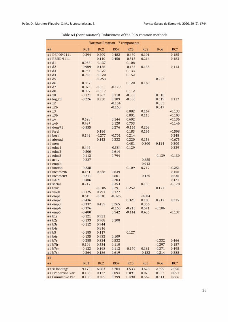
We considered 8 significant components, which account for a cumulated variance higher than 70%. Notwithstanding, the main justification for this choice is the theoretical interpretability of the results – see below. We then performed a varimax rotation to the components obtained,6 in order to get each variable associated with higher loads to a single component. For robustness, results for 6 to 10 components, as well as for none rotation, promax, cluster and quartimax rotations for 8 components, were also obtained – the complete results are available in Table A4 in the SM.
Results of the PCA carried out on the matrix composed of the 50 indicators for the 264 Galician rural municipalities are summarized in Table 2, with loadings smaller than |0.2| omitted for clarity. Loadings are the coefficients of each variable in the linear function of a specific component, measuring the importance of such variables in the component. Communality (h2) in factorial analysis represents the part of the variance of a variable that contributes to the formation of the components, and uniqueness (u2) the part that represents its specific behaviour.
Loadings > |0.6| were used to determine the domains that are associated with each component. This way, the results obtained justify, from a theoretical perspective, the number of significant components and rotation techniques used. Indeed, the first rotated component (RC1) is clearly associated to the domain ‘demographic structure’ (which extracts 18% of total variance) and RC2 to the domain ‘business financial results’ (12% of total variance), both with loadings > |0.9| for most indicators. In addition, RC5 and RC3 are also strongly identified with the distance to the main urban areas (domain ‘geographic variables’) and employment rates (domain ‘labour market’). The last three rotated components, RC6 to RC8, which extract 14% of total variance altogether, have significant loadings higher than |0.6| for most indicators in the domains ‘geographic variables’ (population of the county capital and distance to it), population (foreign people, born in the municipality and outside Galicia) and business density.
6 For such purpose, we used the command principal in the package psych of the R statistical suite (Revelle, 2017).

Peón, D., Martínez-Filgueira, X. M., & López-Iglesias, E. Revista Galega de Economía 2020, 29 (2), 6744
12
Table 2. Principal component analysis (PCA) factor loadings
Loadings:
RC1 RC2 RC4 RC5 RC3 RC6 RC7 RC8 h2 u2
DEPOP.91-11 -0.40 0.50 -0.49 0.75 0.25 RESID.91-11 0.46 -0.51 0.20 0.58 0.42 d1 0.96 0.97 0.03 d2 -0.92 0.90 0.10 d3 0.96 0.96 0.05 d4 0.94 0.92 0.08 d5 -0.41 0.22 0.78
d6 0.84 0.76 0.24 d7 0.88 0.82 0.18 d8 0.91 0.86 0.14
x0 0.24 -0.48 0.57 0.64 0.36 log_x0 0.24 -0.50 0.61 0.73 0.27 x2 0.87 0.81 0.19 x2b 0.88 0.83 0.17 x3 0.89 0.85 0.15 x3b 0.90 0.85 0.15 x4 0.52 0.69 0.21 0.82 0.19 x4b 0.49 0.75 0.20 0.86 0.14 dens91 -0.54 0.29 0.24 0.48 0.52
forei 0.72 0.60 0.40 born -0.25 0.61 0.23 -0.45 0.72 0.28
abroad 0.22 0.85 0.82 0.18 men 0.49 -0.29 -0.32 0.44 0.56 educ1 0.41 -0.32 0.40 0.53 0.47
educ2 -0.47 0.58 -0.26 0.69 0.31 educ3 0.74 -0.20 0.26 0.69 0.31 activ -0.23 -0.86 0.80 0.20 emplo -0.93 0.88 0.12 unemp -0.22 0.75 0.69 0.32 income96 0.22 0.66 0.52 0.48
income09 0.73 -0.36 0.74 0.26 ISDN -0.40 0.31 -0.37 0.40 0.60 social 0.20 0.29 0.36 0.26 0.74 tour 0.32 0.23 -0.21 0.23 0.77
work 0.73 0.25 0.67 0.33 emp1 0.61 -0.31 -0.62 0.90 0.10 emp2 -0.42 0.33 0.20 -0.25 0.43 0.57 emp3 -0.33 0.45 0.25 0.36 0.53 0.47
emp4 -0.40 0.52 0.32 0.62 0.39 emp5 -0.46 0.49 0.48 0.77 0.23
b1r 0.96 0.94 0.06 b2r 0.93 0.90 0.10 b3r 0.98 0.97 0.03 b4r 0.88 0.78 0.22 b5 0.08 0.92
b6r 0.93 0.92 0.08 b7r -0.31 0.63 0.53 0.86 0.14 b7ir 0.39 0.61 0.58 0.43
b7cr 0.22 0.71 0.64 0.36 b7sr 0.37 0.70 0.26 0.77 0.23
Peón, D., Martínez-Filgueira, X. M., & López-Iglesias, E. Revista Galega de Economía 2020, 29 (2), 6744
13
Table 2 (continuation). Principal component analysis (PCA) factor loadings
RC1 RC2 RC4 RC5 RC3 RC6 RC7 RC8
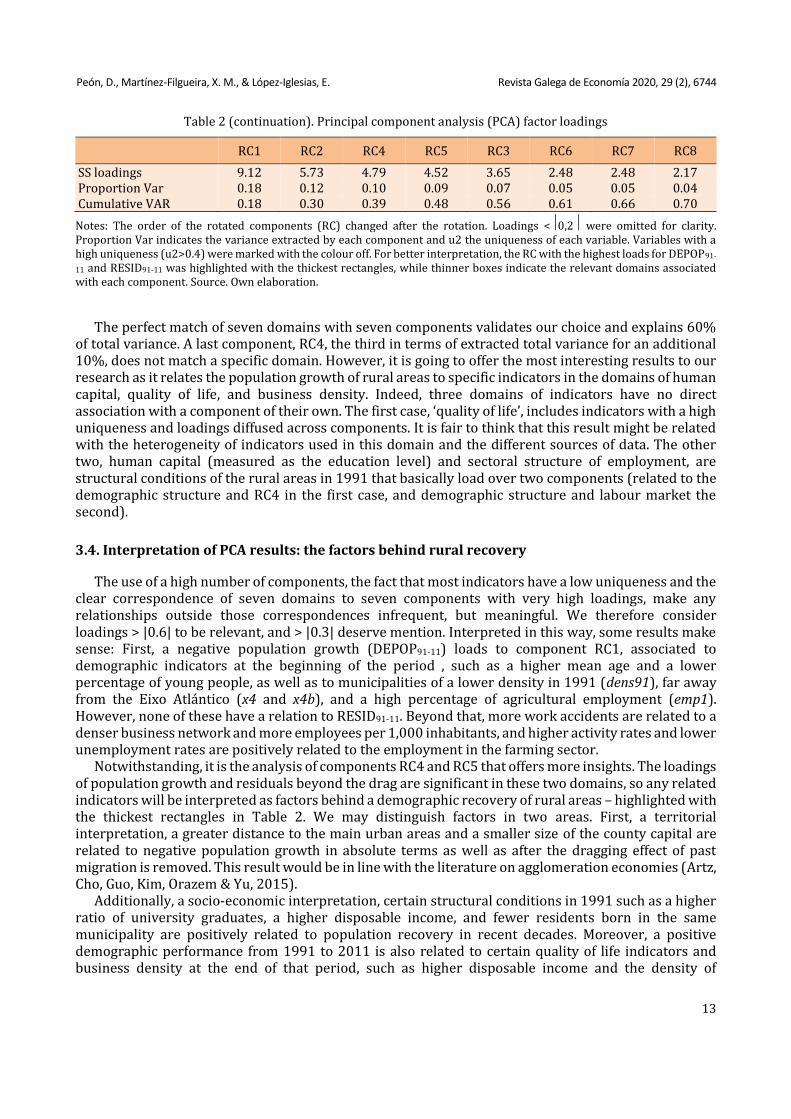
SS loadings 9.12 5.73 4.79 4.52 3.65 2.48 2.48 2.17 Proportion Var 0.18 0.12 0.10 0.09 0.07 0.05 0.05 0.04 Cumulative VAR 0.18 0.30 0.39 0.48 0.56 0.61 0.66 0.70
Notes: The order of the rotated components (RC) changed after the rotation. Loadings <⃒0,2⃒ were omitted for clarity. Proportion Var indicates the variance extracted by each component and u2 the uniqueness of each variable. Variables with a high uniqueness (u2>0.4) were marked with the colour off. For better interpretation, the RC with the highest loads for DEPOP91-
11 and RESID91-11 was highlighted with the thickest rectangles, while thinner boxes indicate the relevant domains associated with each component. Source. Own elaboration.
The perfect match of seven domains with seven components validates our choice and explains 60% of total variance. A last component, RC4, the third in terms of extracted total variance for an additional 10%, does not match a specific domain. However, it is going to offer the most interesting results to our research as it relates the population growth of rural areas to specific indicators in the domains of human capital, quality of life, and business density. Indeed, three domains of indicators have no direct association with a component of their own. The first case, ‘quality of life’, includes indicators with a high uniqueness and loadings diffused across components. It is fair to think that this result might be related with the heterogeneity of indicators used in this domain and the different sources of data. The other two, human capital (measured as the education level) and sectoral structure of employment, are structural conditions of the rural areas in 1991 that basically load over two components (related to the demographic structure and RC4 in the first case, and demographic structure and labour market the second).
3.4. Interpretation of PCA results: the factors behind rural recovery
The use of a high number of components, the fact that most indicators have a low uniqueness and the clear correspondence of seven domains to seven components with very high loadings, make any relationships outside those correspondences infrequent, but meaningful. We therefore consider loadings > |0.6| to be relevant, and > |0.3| deserve mention. Interpreted in this way, some results make sense: First, a negative population growth (DEPOP91-11) loads to component RC1, associated to demographic indicators at the beginning of the period , such as a higher mean age and a lower percentage of young people, as well as to municipalities of a lower density in 1991 (dens91), far away from the Eixo Atlántico (x4 and x4b), and a high percentage of agricultural employment (emp1). However, none of these have a relation to RESID91-11. Beyond that, more work accidents are related to a denser business network and more employees per 1,000 inhabitants, and higher activity rates and lower unemployment rates are positively related to the employment in the farming sector.
Notwithstanding, it is the analysis of components RC4 and RC5 that offers more insights. The loadings of population growth and residuals beyond the drag are significant in these two domains, so any related indicators will be interpreted as factors behind a demographic recovery of rural areas – highlighted with the thickest rectangles in Table 2. We may distinguish factors in two areas. First, a territorial interpretation, a greater distance to the main urban areas and a smaller size of the county capital are related to negative population growth in absolute terms as well as after the dragging effect of past migration is removed. This result would be in line with the literature on agglomeration economies (Artz, Cho, Guo, Kim, Orazem & Yu, 2015).
Additionally, a socio-economic interpretation, certain structural conditions in 1991 such as a higher ratio of university graduates, a higher disposable income, and fewer residents born in the same municipality are positively related to population recovery in recent decades. Moreover, a positive demographic performance from 1991 to 2011 is also related to certain quality of life indicators and business density at the end of that period, such as higher disposable income and the density of
Peón, D., Martínez-Filgueira, X. M., & López-Iglesias, E. Revista Galega de Economía 2020, 29 (2), 6744
14
companies and freelancers in the services sector. Other noteworthy factors, with loadings >|0.3|, are higher ratio of employment in the services sector in 1991, as well as quality of life indicators in 2011 such as the access to ISDN services, places in social services centres, and the number of beds in hotels and campsites. Two other results are related to the education level (illiterate population and secondary education), but both are correlated with the demographic structure in component RC1, since younger municipalities are expected to have more people with a secondary education and fewer with no studies.
Therefore, the debate is still open regarding the dichotomy “fostering entrepreneurship in rural areas versus ensuring higher quality of life standards for residents there”. On one hand, there is a clear result in favour of a denser business network in the tertiary sector –particularly in the form of self-employment– as a consequence, but we found no evidence on business financial results. On the other, there is a positive impact of having more university graduates and higher disposable income, but quality of life indicators such as proxies for the access to public services and the presence of amenities only offer weak correlations at period end. All these results are robust to alternative rotation techniques –see Table A4 in the SM. Thus, results are qualitatively similar for all methods considered, and they are quantitatively even more important with a cluster rotation (in particular, higher loadings by tertiary education level, distance to urban areas, and business density in the services sector).
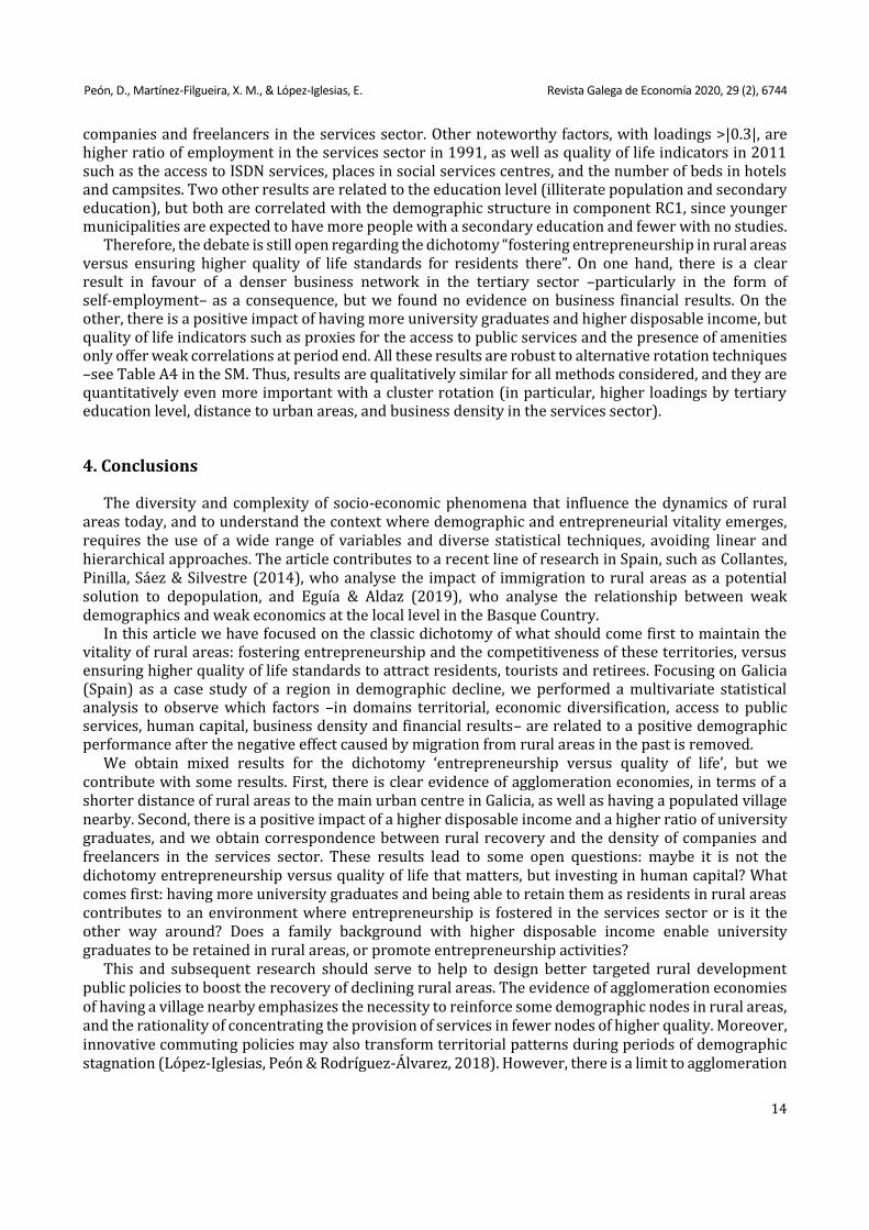
4. Conclusions
The diversity and complexity of socio-economic phenomena that influence the dynamics of rural areas today, and to understand the context where demographic and entrepreneurial vitality emerges, requires the use of a wide range of variables and diverse statistical techniques, avoiding linear and hierarchical approaches. The article contributes to a recent line of research in Spain, such as Collantes, Pinilla, Sáez & Silvestre (2014), who analyse the impact of immigration to rural areas as a potential solution to depopulation, and Eguía & Aldaz (2019), who analyse the relationship between weak demographics and weak economics at the local level in the Basque Country.
In this article we have focused on the classic dichotomy of what should come first to maintain the vitality of rural areas: fostering entrepreneurship and the competitiveness of these territories, versus ensuring higher quality of life standards to attract residents, tourists and retirees. Focusing on Galicia (Spain) as a case study of a region in demographic decline, we performed a multivariate statistical analysis to observe which factors –in domains territorial, economic diversification, access to public services, human capital, business density and financial results– are related to a positive demographic performance after the negative effect caused by migration from rural areas in the past is removed.
We obtain mixed results for the dichotomy ‘entrepreneurship versus quality of life’, but we contribute with some results. First, there is clear evidence of agglomeration economies, in terms of a shorter distance of rural areas to the main urban centre in Galicia, as well as having a populated village nearby. Second, there is a positive impact of a higher disposable income and a higher ratio of university graduates, and we obtain correspondence between rural recovery and the density of companies and freelancers in the services sector. These results lead to some open questions: maybe it is not the dichotomy entrepreneurship versus quality of life that matters, but investing in human capital? What comes first: having more university graduates and being able to retain them as residents in rural areas contributes to an environment where entrepreneurship is fostered in the services sector or is it the other way around? Does a family background with higher disposable income enable university graduates to be retained in rural areas, or promote entrepreneurship activities?
This and subsequent research should serve to help to design better targeted rural development public policies to boost the recovery of declining rural areas. The evidence of agglomeration economies of having a village nearby emphasizes the necessity to reinforce some demographic nodes in rural areas, and the rationality of concentrating the provision of services in fewer nodes of higher quality. Moreover, innovative commuting policies may also transform territorial patterns during periods of demographic stagnation (López-Iglesias, Peón & Rodríguez-Álvarez, 2018). However, there is a limit to agglomeration

Peón, D., Martínez-Filgueira, X. M., & López-Iglesias, E. Revista Galega de Economía 2020, 29 (2), 6744
15
economies, too. At different levels, different responses are required. To avoid territorial exclusion, improving information systems and telematics interconnection, creating mobile units for social and health assistance, and prioritizing prevention might be different alternatives (Fernández & Peón, 2017). Finally, public policies in support of business activities should pay attention to the barriers they face, such as financial constraints, qualified personnel, and uneven market competition (Peón & Martínez Filgueira, 2019).
The main limitation of our research, both in terms of interpreting the results obtained and to answer some of these open questions, comes from the lack of data for Galicia at the municipal level. Moreover, the results of the statistical analysis should not be interpreted in terms of causality, but of association or relationship among variables. Indeed, PCA is an exploratory analysis, and this is the reason why no ex-ante testable hypotheses were defined. However, the methodology and results obtained could serve as a starting point in future research analysis for this and other regions, in terms of choosing the appropriate variables to be included in the econometric models.
Appendix 1. Supplementary material
Table A1. Correlations between population change 1950-1991, demographic structure in 1991, and population change 1911-2011(*)
EMIG. 5091 DEPOP.9111 d1 d2 d3 d4 d5 d6 d7 d8
EMIG.5091 1.00 0.65 -0.89 0.86 -0.89 -0.83 -0.16 -0.78 -0.76 -0.81 DEPOP.9111 0.65 1.00 -0.64 0.65 -0.63 -0.61 -0.14 -0.49 -0.54 -0.58
d1 -0.89 -0.64 1.00 -0.98 0.99 0.96 0.21 0.84 0.91 0.92 d2 0.86 0.65 -0.98 1.00 -0.94 -0.93 -0.19 -0.73 -0.87 -0.91 d3 -0.89 -0.63 0.99 -0.94 1.00 0.96 0.19 0.91 0.87 0.90 d4 -0.83 -0.61 0.96 -0.93 0.96 1.00 0.17 0.86 0.86 0.93 d5 -0.16 -0.14 0.21 -0.19 0.19 0.17 1.00 0.17 0.18 0.14 d6 -0.78 -0.49 0.84 -0.73 0.91 0.86 0.17 1.00 0.74 0.77 d7 -0.76 -0.54 0.91 -0.87 0.87 0.86 0.18 0.74 1.00 0.86 d8 -0.81 -0.58 0.92 -0.91 0.90 0.93 0.14 0.77 0.86 1.00
Note: (*) Variables are described in Table A3. Source: Own elaboration. Data: INE, Census 1950, 1991, 2011.
Table A2. Regressions DEPOP91-11 as a function of one or more regressors
1 regressor
Peón, D., Martínez-Filgueira, X. M., & López-Iglesias, E. Revista Galega de Economía 2020, 29 (2), 6744
16
Table A2 (continuation). Regressions DEPOP91-11 as a function of one or more regressors
2 regressors
The R2 for regression DEPOP91-11 = f(EMIG50-91) is almost identical to that with the best results –the regression that uses d2 as a regressor:
Estimate Std. Error t value Pr(>|t|)
(Intercept) -0.14373 0.07558 -1.902 0.0581 . EMIG.50-91 0.83423 0.05558 15.009 <2e-16***
---
Signif. codes: 0 ‘***’ 0.001 ‘**’ 0.01 ‘*’ 0.05 ‘.’ 0.1 ‘ ’ 1 Residual standard error: 1.053 on 313 degrees of freedom Multiple R-squared: 0.4185, Adjusted R-squared: 0.4166 F-statistic: 225.3 on 1 and 313 DF, p-value: < 2.2e-16 ###############################################################
Estimate Std. Error t value Pr(>|t|)
(Intercept) -4.73187 0.26209 -18.05 <2e-16*** demografia.d2 0.17221 0.01132 15.22 <2e-16***
---
Signif. codes: 0 ‘***’ 0.001 ‘**’ 0.01 ‘*’ 0.05 ‘.’ 0.1 ‘ ’ 1 Residual standard error: 1.047 on 313 degrees of freedom Multiple R-squared: 0.4252, Adjusted R-squared: 0.4234 F-statistic: 231.6 on 1 and 313 DF, p-value: < 2.2e-16
Peón, D., Martínez-Filgueira, X. M., & López-Iglesias, E. Revista Galega de Economía 2020, 29 (2), 6744
17
In adition, combining d2 and EMIG50-91 does not add much –regressors are correlated:
Estimate Std. Error t value Pr(>|t|)
(Intercept) -2.67832 0.56572 -4.734 3.34e-06*** EMIG.50-91 0.42726 0.10498 4.070 5.97e-05***
demografia.d2 0.09714 0.02150 4.518 8.85e-06***
---
Signif. codes: 0 ‘***’ 0.001 ‘**’ 0.01 ‘*’ 0.05 ‘.’ 0.1 ‘ ’ 1 Residual standard error: 1.022 on 312 degrees of freedom Multiple R-squared: 0.4542, Adjusted R-squared: 0.4507 F-statistic: 129.8 on 2 and 312 DF, p-value: < 2.2e-16
###############################################################
It would make sense to combine EMIG50-91 and d5, since the latter –the 85+ over 65+ ratio- is the only demographic indicator
that is not correlated to EMIG50-91 (hence, this does not work as a good proxy of it). However, the regression does not add much, d5 results not significant, and adj-R2 values worsen.
Estimate Std. Error t value Pr(>|t|)
(Intercept) 0.11513 0.32763 0.351 0.726 EMIG.50-91 0.82711 0.05630 14.691 <2e-16***
demografia.d5 -0.02769 0.03410 -0.812 0.417 .
---
Signif. codes: 0 ‘***’ 0.001 ‘**’ 0.01 ‘*’ 0.05 ‘.’ 0.1 ‘ ’ 1 Residual standard error: 1.054 on 312 degrees of freedom Multiple R-squared: 0.4197, Adjusted R-squared: 0.416 F-statistic: 112.8 on 2 and 312 DF, p-value: < 2.2e-16
Table A3. Variables used in the analysis
Type Name Indicator Description - estimation Source
Population growth
EMIG.50-91 Emigration in years 1950 to 1991
Annualized percentage of population growth rate (population 1991 / population 1950)
INE (census)
DEPOP.91-11 Change in population, 1991 to 2011
Annualized percentage of population growth rate (population 2011 / population 1991)
INE (census)
RESID.91-11 Residuals of the demographic drag, 1991-2011
Annualized percentage of population growth rate above (below) regression estimates
Own / INE
Demographic structure
d1 Mean age Arithmetic average of all the inhabitants' age by January 1st, 1991
IGE
d2 % population under 20
Population under 20 years old over total population, year 1991
IGE
d3 % population aged 65 and more
Population aged 65 and more over total population, year 1991
IGE
d4 Elderly dependency ratio
Population aged 65 and more / population under 20, year 1991
IGE
d5 85+ over 65+ Population aged 85+ / population aged 65+, year 1991
IGE
d6 Age-dependency ratio
Dependent population (under 15; 65 and more) / population 15-64, year 1991
IGE
d7 Labour force structure
Population 40-64 years old / population 15-39 years old, year 1991
IGE
d8 Labour force replacement
Population 60-64 years old / population 15-19 years old, year 1991
IGE
Peón, D., Martínez-Filgueira, X. M., & López-Iglesias, E. Revista Galega de Economía 2020, 29 (2), 6744
18
Table A3 (continuation). Variables used in the analysis
Type Name Indicator Description - estimation Source
Geographic variables
x0 Population of the county capital
Number of inhabitants of the municipality capital of county
IGE
x2 Distance to the county capital Distance to the county capital (km) Googlemaps
x2b Ibidem, in minutes driving by road
x3 Distance to the closest city
Distance to the closest city (+50.000 inhababitants) in km Googlemaps
x3b Ibidem, in minutes driving by road
x4 Distance county capital - Eixo Atlántico
Distance in kilometers to the Eixo Atlántico (proxy: closest airport) Googlemaps
x4b Ibidem, in minutes driving by road
Population
dens91 Population density in 1991 Total population in the 1991 census / km2 INE, IGE
forei Resident foreign people (%) Percentage of foreign residents to total population, year 1991
INE (census)
born Born in the municipality (%)
Percentage of residents that were born in the municipality to total population, year 1991
INE (census)
abroad Born outside Galicia (%) Percentage of residents that were born outside Galicia to total population, year 1991
INE (census)
men Percentage of men Percentage of men to total population, year 1991
INE (census)
Education
educ1 Illiterate population & no formal degree (%)
Illiterate people and literate without formal education degree to total population, year 1991
INE (census)
educ2 Population with secondary education (%)
Number of residents with a secondary education degree to total population, year 1991
INE (census)
educ3 Population with tertiary level education (%)
Number of residents with a university degree to total population, year 1991
INE (census)
Labour market
activ Activity rate Percentage of active resident population to total population aged 16 or older, year 1991
INE, IGE
emplo Employment rate Percentage of occupied residents to total population aged 16 or older, year 1991
INE, IGE
unemp Unemployment rate Percentage of unemployed residents to total population aged 16 or older, year 1991
INE, IGE
Quality of life
income96 Disposable income per capita
Average disposable income per number of residents in the municipality, year 1996
IGE
income09 Disposable income per capita
Average disposable income per number of residents in the municipality, year 2009
IGE
ISDN Access to ISDN services Percentage of residents with access to Integrated Services Digital Network, year 2011
Mº Hacienda, IGE
social Places in social services / 1,000 inhabs
Number of places in social services centers (elder people, disabilities, minors, family, immigrants and community services) per 1,000 residents, year 2011
C.Traballo, IGE
tour Beds in hotels and campings to population
Number of beds in hotels, rural houses and campsites, pero 1,000 residents, year 2011
C.Cultura, IGE
work work accidents / 1,000 inhabs
Number of work accidents with registered leave, per 1,000 residents, year 2001
C.Traballo, IGE
Peón, D., Martínez-Filgueira, X. M., & López-Iglesias, E. Revista Galega de Economía 2020, 29 (2), 6744
19
Table A3 (continuation). Variables used in the analysis
Type Name Indicator Description - estimation Source
Employment structure
emp1 Employees in farming (%) Residents employed in the farming sector to total number of employed residents, year 1991
IGE
emp2 Employees in fishing (%) Residents employed in the fishing sector to total number of employed residents, year 1991
IGE
emp3 Employees in industry (%) Residents employed in the industrial sector to total number of employed residents, year 1991
IGE
emp4 Employees in construction (%) Residents employed in the construction sector to total number of employed residents, year 1991
IGE
emp5 Employees in services (%) Residents employed in the services sector to total number of employd residents, year 1991
IGE
Business Financial results
b1r Total sales revenues to population
Sum of firms' sales revenues average 2001-2010, divided by municipality's population in year 2011
SABI
b2r Total assets to population Sum of firms' total assets average 2001-2010, divided by municipality's population in year 2011
SABI
b3r Total equity to population Sum of firms' equity average 2001-2010, divided by municipality's population in year 2011
SABI
b4r Sum of earnings before taxes to population
Sum of firms' EBT average 2001-2010, divided by municipality's population in year 2011
SABI
b5 Average ROA Firms' average return on assets over years 2001-2010
SABI
b6r Total employees to population Total number of employees, average 2001-2010, divided by municipality's population in year 2011
SABI
Business density
b7r Number of firms / 1,000 inhabs
Ratio total number of firms in the council (year 2010) per 1,000 inhabitants (census year 2011)
IGE
b7ir Firms in industrial sectors / 1,000 inhabs
Ratio number of firms in industrial sectors (year 2010) per 1,000 inhabs. (census year 2011)
IGE
b7cr Firms in construction sector / 1,000 inhabs
Ratio number of firms in construction sector (year 2010) per 1,000 inhabs. (census year 2011)
IGE
b7sr Firms in services sector / 1,000 inhabs
Ratio number of firms in services sector (year 2010) per 1,000 inhabitants (census year 2011)
IGE
Mº Hacienda stands for Spanish Treasury, C.Traballo and C.Cultura stand for Galician Ministry of Work and of Culture, respectively. INE is the Spanish Statistics Institute, IGE the Galician Statistics Institute, and SABI stands for SABI – Bureau van Dijk database. Data treatment: For population growth, we use population data from the INE censuses of 1950, 1991 e 2011. We take into account all changes in the municipality map since 1950 following Míguez (2013). For the 1950 census we consider de jure population, and we sum the population in 1950 of councils when these merged afterwards. These include Buxán added to Val do Dubra, A Enfesta to Santiago de Compostela, Neira de Jusá to Baralla; Riobarba to O Vicedo; Vilaodrid to A Pontenova. Acebedo del Río to Celanova, Rio to San Xoan de Rio, and Pontesampaio to Pontevedra. In addition, we allot population between councils, according to their population in the 1991 census, when these split. This includes Cariño from Ortigueira in 1988. Finally, a typo in Narón data was amended: according to de jure population, its inhabitants in year 1950 were 14,895. For the 1950 and 1991 census we allot population between councils that split after 1991 according to their population in the 2001 census. These include the split of Burela from Cervo in 1994, and A Illa de Arousa from Vilanova de Arousa in 1996. For data on demographic structure, population and labour market, which refer to year 1991, for those two new-born councils in 1994 and 1996 we took the same data of the councils from which they split. In regards to distances by road from county capitals to county capitals, Galician cities and the Eixo Atlántico –using the closest of the three Galician airports as a proxy- we selected the quickest route according to googlemaps, as it takes the quality of the roads into account, and measured the distance in kilometers and driving time in minutes for that route. INE statistics about education level (from which we estimated indicators e1, e2 and e3) omit some data for 23 councils when “only a few sample observations were available”. In such case we allot any missing population among the education levels with no data using Galician averages. This basically afected solely our estimations of indicator e3 for 22 of those 23 councils. Finally, data on GVA as a percentage of county's GDP, uses data available at the county level and assumes the same structure for its municipalities. Source: Own elaboration.

Peón, D., Martínez-Filgueira, X. M., & López-Iglesias, E. Revista Galega de Economía 2020, 29 (2), 6744
20
Table A4. Robustness of the PCA rotation methods
Varimax Rotation – 10 components
## RC1 RC2 RC5 RC4 RC3 RC6 RC7 RC8 RC10 RC9
## DEPOP.9111 -0.461 0.164 -0.384 0.351 0.138 0.152 0.507 -0.153 ## RESID.9111 -0.393 0.298 0.167 0.105 0.111 0.578 -0.232 ## d1 0.963 -0.121 0.101 -0.112 ## d2 -0.929 0.105 -0.118 0.106 ## d3 0.956 -0.116 0.131 ## d4 0.938 0.141 ## d5 -0.116 -0.165 0.113 0.647 ## d6 0.819 0.136 0.148 0.173 ## d7 0.856 -0.244 0.116 ## d8 0.902 0.108 -0.118 ## x0 -0.136 0.239 -0.435 0.116 0.573 0.130 -0.184 ## log_x0 -0.256 0.172 -0.455 0.609 0.180 -0.152 ## x2 0.111 -0.137 0.887 -0.139 0.126 ## x2b 0.102 -0.175 0.885 0.140 ## x3 0.901 0.133 -0.128 ## x3b 0.909 ## x4 0.523 0.712 0.127 -0.123 ## x4b 0.490 0.771 -0.121 ## dens91 -0.537 -0.180 0.230 0.203 0.270 ## forei 0.111 0.252 -0.719 ## born 0.148 -0.251 0.145 -0.667 0.299 -0.261 0.130 ## abroad 0.301 0.286 -0.767 0.137 -0.152 ## men 0.469 -0.215 0.449 -0.125 -0.220 -0.320 ## educ1 0.359 -0.114 0.207 -0.428 -0.156 0.116 0.137 0.101 -0.411 ## educ2 -0.437 0.118 -0.122 0.669 0.164 ## educ3 0.840 -0.133 ## activ -0.213 -0.864 ## emplo -0.943 ## unemp -0.209 0.786 -0.130 -0.197 -0.160 ## income96 0.234 0.141 0.472 0.192 0.477 ## income09 -0.208 0.105 0.566 -0.157 0.502 0.223 0.200 ## ISDN -0.445 0.132 0.447 0.266 ## social 0.151 0.154 -0.296 0.474 ## tour 0.194 0.238 0.113 0.550 ## work -0.152 0.741 0.138 -0.119 0.226 0.134 ## emp1 0.630 -0.189 -0.243 -0.577 -0.129 -0.181 -0.152 ## emp2 -0.477 0.344 -0.142 0.120 0.232 0.234 0.293 ## emp3 -0.368 0.455 0.170 0.332 0.264 ## emp4 -0.398 -0.209 -0.213 0.491 -0.207 0.363 ## emp5 -0.439 -0.124 0.560 0.486 -0.107 0.129 ## b1r 0.956 ## b2r -0.117 0.931 ## b3r 0.979 ## b4r 0.873 ## b5 -0.127 0.113 0.129 -0.441 -0.214 ## b6r -0.124 0.931 0.166 ## b7r -0.279 0.209 0.510 -0.101 0.155 0.719 ## b7ir 0.400 -0.173 0.615 -0.154 ## b7cr -0.165 -0.139 0.800 ## b7sr -0.327 0.139 0.646 -0.120 0.224 0.473
## ## RC1 RC2 RC5 RC4 RC3 RC6 RC7 RC8 RC10 RC9
## ss loadings 9.060 5.803 4.385 4.177 3.537 2.427 2.339 2.336 1.886 1.559 ## Proportion Var 0.181 0.116 0.088 0.084 0.071 0.049 0.047 0.047 0.038 0.031 ## Cumulative Var 0.181 0.297 0.385 0.469 0.539 0.588 0.635 0.681 0.719 0.750

Peón, D., Martínez-Filgueira, X. M., & López-Iglesias, E. Revista Galega de Economía 2020, 29 (2), 6744
21
Table A4 (continuation). Robustness of the PCA rotation methods
Varimax Rotation – 9 components
## RC1 RC2 RC4 RC5 RC3 RC6 RC7 RC8 RC9
## DEPOP.9111 -0.409 0.162 0.477 -0.479 0.169 0.249 ## RESID.9111 0.447 -0.507 0.203 0.136 0.242 ## d1 0.962 -0.120 -0.103 ## d2 -0.920 0.106 -0.123 0.100 0.123 ## d3 0.955 -0.115 0.126 ## d4 0.935 0.140 ## d5 -0.107 -0.102 -0.188 0.645 ## d6 0.829 0.117 0.156 0.101 0.161 ## d7 0.870 -0.209 ## d8 0.909 ## x0 -0.121 0.234 0.132 -0.486 0.103 0.562 -0.139 ## log_x0 -0.235 0.168 0.131 -0.509 0.605 ## x2 -0.149 0.120 0.868 -0.101 ## x2b -0.177 0.102 0.877 ## x3 0.891 0.146 0.148 ## x3b 0.901 0.113 ## x4 0.530 0.140 0.692 0.168 -0.103 ## x4b 0.499 0.104 0.754 0.161 ## dens91 -0.553 0.100 0.240 -0.170 0.204 0.255 ## forei 0.113 0.220 0.734 ## born 0.148 -0.244 -0.660 0.209 -0.400 ## abroad 0.215 0.250 0.107 0.824 ## men 0.105 0.462 -0.209 0.100 -0.416 -0.126 -0.404 ## educ1 0.418 -0.112 -0.322 0.154 -0.143 0.151 0.303 -0.301 ## educ2 -0.472 0.111 0.611 -0.112 -0.135 -0.218 ## educ3 0.792 -0.183 0.175 -0.146 ## activ -0.220 -0.868 ## emplo -0.944 ## unemp -0.225 0.778 0.113 -0.233 -0.110 ## income96 0.122 0.233 0.616 0.237 0.163 ## income09 -0.194 0.692 -0.139 -0.407 0.178 ## ISDN -0.395 0.269 -0.381 0.132 ## social 0.185 0.245 0.373 0.180 0.259 ## tour 0.240 0.245 0.448 ## work -0.139 0.743 0.108 0.104 0.147 0.247 ## emp1 0.632 -0.190 -0.266 -0.585 -0.103 -0.118 -0.168 ## emp2 -0.439 0.326 0.146 0.169 -0.216 0.353 ## emp3 -0.341 0.455 0.231 0.350 0.110 ## emp4 -0.420 -0.228 -0.187 0.473 0.154 0.347 ## emp5 -0.470 0.505 -0.127 0.485 0.144 -0.118 ## b1r -0.101 0.954 ## b2r -0.119 0.930 0.100 ## b3r 0.978 ## b4r 0.871 ## b5 -0.169 0.124 -0.127 -0.399 ## b6r -0.130 0.931 0.101 0.135 ## b7r -0.315 0.205 0.579 -0.115 -0.154 -0.116 0.567 ## b7ir 0.402 0.187 0.587 -0.135 ## b7cr -0.180 0.122 -0.137 -0.124 0.758 ## b7sr -0.365 0.132 0.681 -0.131 -0.133 -0.176 0.300
## ## RC1 RC2 RC4 RC5 RC3 RC6 RC7 RC8 RC9
## ss loadings 9.198 5.776 4.630 4.501 3.567 2.471 2.427 2.188 1.542 ## Proportion Var 0.184 0.116 0.093 0.090 0.071 0.049 0.049 0.044 0.031 ## Cumulative Var 0.184 0.299 0.392 0.482 0.553 0.603 0.651 0.695 0.726

Peón, D., Martínez-Filgueira, X. M., & López-Iglesias, E. Revista Galega de Economía 2020, 29 (2), 6744
22
Table A4 (continuation). Robustness of the PCA rotation methods
Varimax Rotation – 8 components, complete results
## RC1 RC2 RC4 RC5 RC3 RC6 RC7 RC8 h2 u2 com
## DEPOP.9111 -0.40 0.16 0.50 -0.49 0.18 0.09 0.01 0.20 0.75 0.250 3.8 ## RESID.9111 0.08 0.08 0.46 -0.51 0.19 0.14 0.01 0.20 0.58 0.416 2.9 ## d1 0.96 -0.12 -0.11 0.10 -0.03 -0.01 0.03 -0.06 0.97 0.033 1.1 ## d2 -0.91 0.10 0.10 -0.13 0.13 0.02 -0.06 0.10 0.90 0.097 1.2 ## d3 0.96 -0.11 -0.07 0.13 0.03 -0.01 0.03 -0.04 0.96 0.045 1.1 ## d4 0.94 -0.09 -0.07 0.14 0.02 0.00 0.01 -0.10 0.92 0.078 1.1 ## d5 0.09 -0.13 0.06 0.01 0.02 0.05 -0.16 -0.41 0.22 0.779 1.7 ## d6 0.84 -0.09 0.00 0.12 0.17 0.02 -0.03 0.03 0.76 0.243 1.2 ## d7 0.87 -0.10 -0.20 -0.04 0.01 -0.02 -0.02 -0.01 0.82 0.184 1.1 ## d8 0.91 -0.08 -0.06 0.10 -0.08 0.00 -0.02 -0.10 0.86 0.141 1.1 ## x0 -0.13 0.24 0.10 -0.48 0.07 0.57 0.04 0.00 0.64 0.361 2.6 ## log_x0 -0.24 0.17 0.12 -0.50 0.03 0.61 -0.02 0.07 0.73 0.271 2.6 ## x2 0.05 -0.01 -0.14 0.14 -0.06 0.87 -0.02 -0.12 0.81 0.191 1.2 ## x2b 0.05 0.06 -0.16 0.12 -0.03 0.88 0.03 -0.12 0.83 0.169 1.2 ## x3 0.09 0.02 -0.04 0.89 0.15 0.01 0.17 0.01 0.85 0.150 1.2 ## x3b 0.07 0.04 -0.03 0.90 0.10 0.07 0.13 -0.02 0.85 0.154 1.1 ## x4 0.52 0.03 0.12 0.69 0.03 -0.03 0.21 0.01 0.81 0.191 2.2 ## x4b 0.49 0.03 0.10 0.75 0.01 0.01 0.20 -0.04 0.86 0.142 2.0 ## dens91 -0.54 0.09 0.29 -0.18 0.24 -0.01 -0.07 -0.09 0.48 0.518 2.5 ## forei -0.03 0.10 -0.09 0.19 0.11 0.06 0.72 0.07 0.60 0.396 1.3 ## born 0.15 -0.25 -0.61 0.23 -0.06 0.00 -0.45 -0.01 0.72 0.284 2.7 ## abroad 0.01 0.07 0.15 0.22 0.10 -0.02 0.85 0.02 0.82 0.184 1.2 ## men 0.04 0.07 0.05 0.49 -0.29 0.08 -0.32 -0.01 0.44 0.561 2.6 ## educ1 0.40 -0.11 -0.32 0.18 -0.16 0.16 -0.11 0.40 0.53 0.469 4.3 ## educ2 -0.47 0.12 0.58 -0.13 -0.01 -0.15 0.10 -0.26 0.69 0.308 2.8 ## educ3 -0.09 -0.03 0.74 0.00 0.00 -0.20 0.26 -0.17 0.69 0.309 1.6 ## activ -0.23 0.05 0.00 -0.06 -0.86 -0.01 -0.03 -0.05 0.80 0.199 1.2 ## emplo -0.10 0.05 0.02 -0.07 -0.93 0.00 -0.07 0.03 0.88 0.119 1.1 ## unemp -0.22 -0.04 -0.10 0.09 0.75 -0.04 0.15 -0.19 0.69 0.315 1,5 ## income96 0.13 0.22 0.66 0.05 -0.02 0.00 0.06 0.14 0.52 0.476 1.4 ## income09 -0.20 0.03 0.72 0.07 -0.15 0.06 -0.36 0.09 0.74 0.262 1.8 ## ISDN -0.40 0.04 0.31 0.06 -0.06 0.01 -0.37 0.06 0.40 0.598 3.1 ## social 0.20 0.04 0.29 -0.03 0.12 0.01 0.33 0.09 0.26 0.739 3.2 ## tour -0.07 -0.05 0.32 0.23 0.06 0.08 -0.11 -0.21 0.23 0.769 3.5 ## work -0.14 0.73 0.13 0.11 -0.03 0.11 0.13 0.25 0.67 0.327 1.6 ## emp1 0.61 -0.18 -0.31 0.09 -0.62 -0.01 -0.09 -0.03 0.90 0.104 2.7 ## emp2 -0.42 -0.06 0.06 0.33 0.20 0.17 -0.25 -0.09 0.43 0.567 3.8 ## emp3 -0.33 0.45 0.25 -0.08 0.36 0.06 0.08 0.08 0.53 0.471 3.8 ## emp4 -0.40 -0.05 -0.18 -0.20 0.52 -0.04 0.08 0.32 0.62 0.385 3.4 ## emp5 -0.46 0.05 0.49 -0.15 0.48 -0.09 0.18 -0.17 0.77 0.234 3.8 ## b1r -0.11 0.96 0.07 -0.06 -0.04 0.02 -0.01 0.05 0.94 0.063 1.1 ## b2r -0.12 0.93 0.10 0.06 -0.03 0.05 0.07 0.05 0.90 0.100 1.1 ## b3r -0.10 0.98 0.06 0.02 -0.02 0.05 0.03 0.03 0.97 0.028 1.0 ## b4r -0.06 0.88 0.02 -0.05 0.02 0.02 -0.03 -0.04 0.78 0.224 1.0 ## b5 -0.19 0.10 -0.05 0.14 -0.01 0.06 -0.06 0.07 0.08 0.920 3.5 ## b6r -0.13 0.93 0.11 -0.04 -0.03 0.03 0.04 0.16 0.92 0.083 1.1 ## b7r -0.31 0.19 0.63 -0.04 -0.10 -0.15 -0.12 0.53 0.86 0.144 3.0 ## b7ir 0.06 0.38 0.14 -0.02 -0.06 -0.07 0.14 0.61 0.57 0.425 2.0 ## b7cr -0.17 0.01 0.21 -0.14 0.07 -0.11 -0.16 0.71 0.64 0.364 1.6 ## b7sr -0.37 0.13 0.70 0.01 -0.14 -0.14 -0.14 0.26 0.77 0.231 2.2
## ## RC1 RC2 RC4 RC5 RC3 RC6 RC7 RC8
## ss loadings 9.12 5.73 4.79 4.52 3.65 2.48 2.48 2.17 ## Proportion Var 0.18 0.11 0.10 0.09 0.07 0.05 0.05 0.04 ## Cumulative Var 0.18 0.30 0.39 0.48 0.56 0.61 0.66 0.70
## ## Mean item complexity = 2.1 ## Test of the hypothesis that 8 components are sufficient. ## The root mean square of the residuals (RMSR) is 0.04 ## with the empirical chi square 1308.47 with prob < 7.9e-22 ## ## Fit based upon off diagonal values = 0.97
Peón, D., Martínez-Filgueira, X. M., & López-Iglesias, E. Revista Galega de Economía 2020, 29 (2), 6744
23
Table A4 (continuation). Robustness of the PCA rotation methods
Varimax Rotation – 7 components
## RC1 RC2 RC4 RC5 RC3 RC6 RC7
## DEPOP.9111 -0.394 0.209 0.482 -0.489 0.191 0.185 ## RESID.9111 0.140 0.450 -0.515 0.214 0.183 ## d1 0.958 -0.137 0.108 ## d2 -0.909 0.126 -0.135 0.135 0.113 ## d3 0.954 -0.127 0.133 ## d4 0.928 -0.120 0.152 ## d5 -0.253 0.222 ## d6 0.837 0.120 0.169 ## d7 0.873 -0.111 -0.179 ## d8 0.897 -0.117 0.112 ## x0 -0.121 0.267 0.110 -0.505 0.510 ## log_x0 -0.226 0.220 0.109 -0.536 0.519 0.117 ## x2 -0.154 0.835 ## x2b -0.163 0.847 ## x3 0.882 0.167 -0.133 ## x3b 0.891 0.110 -0.103 ## x4 0.528 0.144 0.692 -0.136 ## x4b 0.497 0.120 0.753 -0.146 ## dens91 -0.555 0.276 -0.166 0.208 ## forei 0.186 0.183 0.166 -0.598 ## born 0.142 -0.277 -0.701 0.214 0.248 ## abroad 0.142 0.332 0.220 0.153 -0.675 ## men 0.481 -0.300 0.124 0.300 ## educ1 0.444 -0.384 0.129 0.229 ## educ2 -0.500 0.614 ## educ3 -0.112 0.794 -0.139 -0.130 ## activ -0.227 -0.855 ## emplo -0.913 ## unemp -0.238 0.109 0.717 -0.251 ## income96 0.131 0.258 0.639 0.156 ## income09 -0.211 0.601 -0.175 0.536 ## ISDN -0.406 0.203 0.421 ## social 0.217 0.353 0.139 -0.178 ## tour -0.106 0.291 0.252 0.177 ## work -0.125 0.791 0.127 ## emp1 0.619 -0.181 -0.326 -0.604 ## emp2 -0.436 0.321 0.183 0.217 0.215 ## emp3 -0.337 0.455 0.265 0.356 ## emp4 -0.376 -0.165 -0.215 0.571 -0.186 ## emp5 -0.480 0.542 -0.114 0.435 -0.137 ## b1r -0.121 0.921 ## b2r -0.133 0.908 0.108 ## b3r -0.112 0.944 ## b4r 0.816 ## b5 -0.185 0.117 0.127 ## b6r -0.135 0.932 0.109 ## b7r -0.288 0.324 0.532 -0.332 0.466 ## b7ir 0.109 0.554 0.110 -0.297 0.157 ## b7cr -0.123 0.198 0.112 -0.170 0.161 -0.371 0.495 ## b7sr -0.364 0.186 0.619 -0.132 -0.214 0.388
##
## RC1 RC2 RC4 RC5 RC3 RC6 RC7
## ss loadings 9.172 6.083 4.704 4.533 3.628 2.599 2.556 ## Proportion Var 0.183 0.122 0.094 0.091 0.073 0.052 0.051 ## Cumulative Var 0.183 0.305 0.399 0.490 0.562 0.614 0.666
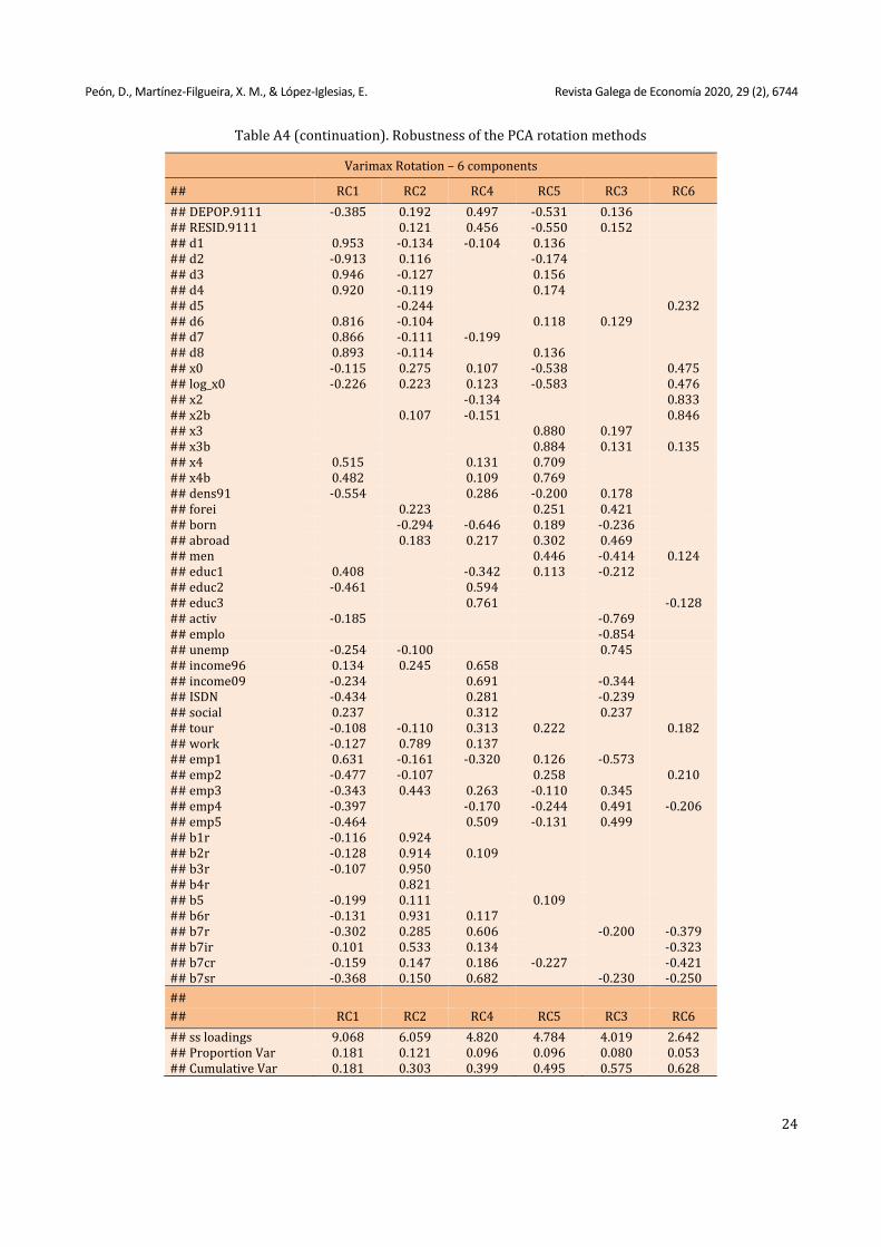
Peón, D., Martínez-Filgueira, X. M., & López-Iglesias, E. Revista Galega de Economía 2020, 29 (2), 6744
24
Table A4 (continuation). Robustness of the PCA rotation methods
Varimax Rotation – 6 components
## RC1 RC2 RC4 RC5 RC3 RC6
## DEPOP.9111 -0.385 0.192 0.497 -0.531 0.136 ## RESID.9111 0.121 0.456 -0.550 0.152 ## d1 0.953 -0.134 -0.104 0.136 ## d2 -0.913 0.116 -0.174 ## d3 0.946 -0.127 0.156 ## d4 0.920 -0.119 0.174 ## d5 -0.244 0.232 ## d6 0.816 -0.104 0.118 0.129 ## d7 0.866 -0.111 -0.199 ## d8 0.893 -0.114 0.136 ## x0 -0.115 0.275 0.107 -0.538 0.475 ## log_x0 -0.226 0.223 0.123 -0.583 0.476 ## x2 -0.134 0.833 ## x2b 0.107 -0.151 0.846 ## x3 0.880 0.197 ## x3b 0.884 0.131 0.135 ## x4 0.515 0.131 0.709 ## x4b 0.482 0.109 0.769 ## dens91 -0.554 0.286 -0.200 0.178 ## forei 0.223 0.251 0.421 ## born -0.294 -0.646 0.189 -0.236 ## abroad 0.183 0.217 0.302 0.469 ## men 0.446 -0.414 0.124 ## educ1 0.408 -0.342 0.113 -0.212 ## educ2 -0.461 0.594 ## educ3 0.761 -0.128 ## activ -0.185 -0.769 ## emplo -0.854 ## unemp -0.254 -0.100 0.745 ## income96 0.134 0.245 0.658 ## income09 -0.234 0.691 -0.344 ## ISDN -0.434 0.281 -0.239 ## social 0.237 0.312 0.237 ## tour -0.108 -0.110 0.313 0.222 0.182 ## work -0.127 0.789 0.137 ## emp1 0.631 -0.161 -0.320 0.126 -0.573 ## emp2 -0.477 -0.107 0.258 0.210 ## emp3 -0.343 0.443 0.263 -0.110 0.345 ## emp4 -0.397 -0.170 -0.244 0.491 -0.206 ## emp5 -0.464 0.509 -0.131 0.499 ## b1r -0.116 0.924 ## b2r -0.128 0.914 0.109 ## b3r -0.107 0.950 ## b4r 0.821 ## b5 -0.199 0.111 0.109 ## b6r -0.131 0.931 0.117 ## b7r -0.302 0.285 0.606 -0.200 -0.379 ## b7ir 0.101 0.533 0.134 -0.323 ## b7cr -0.159 0.147 0.186 -0.227 -0.421 ## b7sr -0.368 0.150 0.682 -0.230 -0.250
##
## RC1 RC2 RC4 RC5 RC3 RC6
## ss loadings 9.068 6.059 4.820 4.784 4.019 2.642 ## Proportion Var 0.181 0.121 0.096 0.096 0.080 0.053 ## Cumulative Var 0.181 0.303 0.399 0.495 0.575 0.628
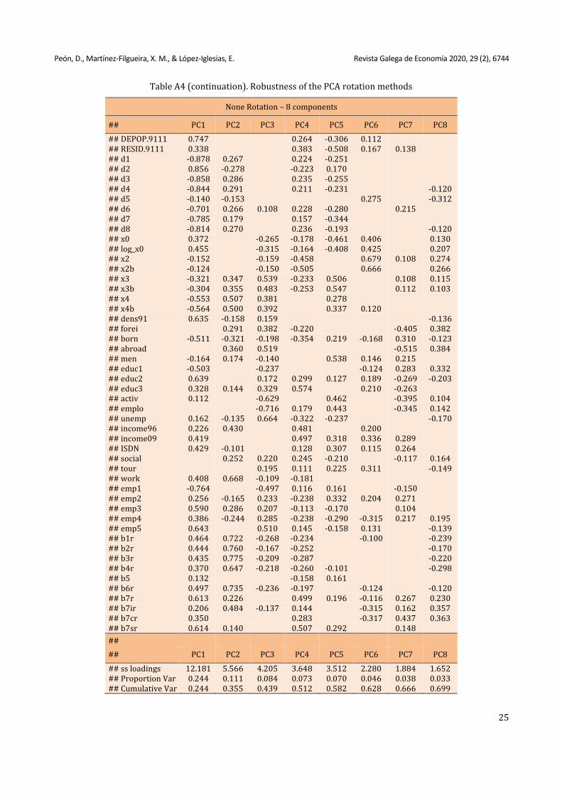
Peón, D., Martínez-Filgueira, X. M., & López-Iglesias, E. Revista Galega de Economía 2020, 29 (2), 6744
25
Table A4 (continuation). Robustness of the PCA rotation methods
None Rotation – 8 components
## PC1 PC2 PC3 PC4 PC5 PC6 PC7 PC8
## DEPOP.9111 0.747 0.264 -0.306 0.112 ## RESID.9111 0.338 0.383 -0.508 0.167 0.138 ## d1 -0.878 0.267 0.224 -0.251 ## d2 0.856 -0.278 -0.223 0.170 ## d3 -0.858 0.286 0.235 -0.255 ## d4 -0.844 0.291 0.211 -0.231 -0.120 ## d5 -0.140 -0.153 0.275 -0.312 ## d6 -0.701 0.266 0.108 0.228 -0.280 0.215 ## d7 -0.785 0.179 0.157 -0.344 ## d8 -0.814 0.270 0.236 -0.193 -0.120 ## x0 0.372 -0.265 -0.178 -0.461 0.406 0.130 ## log_x0 0.455 -0.315 -0.164 -0.408 0.425 0.207 ## x2 -0.152 -0.159 -0.458 0.679 0.108 0.274 ## x2b -0.124 -0.150 -0.505 0.666 0.266 ## x3 -0.321 0.347 0.539 -0.233 0.506 0.108 0.115 ## x3b -0.304 0.355 0.483 -0.253 0.547 0.112 0.103 ## x4 -0.553 0.507 0.381 0.278 ## x4b -0.564 0.500 0.392 0.337 0.120 ## dens91 0.635 -0.158 0.159 -0.136 ## forei 0.291 0.382 -0.220 -0.405 0.382 ## born -0.511 -0.321 -0.198 -0.354 0.219 -0.168 0.310 -0.123 ## abroad 0.360 0.519 -0.515 0.384 ## men -0.164 0.174 -0.140 0.538 0.146 0.215 ## educ1 -0.503 -0.237 -0.124 0.283 0.332 ## educ2 0.639 0.172 0.299 0.127 0.189 -0.269 -0.203 ## educ3 0.328 0.144 0.329 0.574 0.210 -0.263 ## activ 0.112 -0.629 0.462 -0.395 0.104 ## emplo -0.716 0.179 0.443 -0.345 0.142 ## unemp 0.162 -0.135 0.664 -0.322 -0.237 -0.170 ## income96 0.226 0.430 0.481 0.200 ## income09 0.419 0.497 0.318 0.336 0.289 ## ISDN 0.429 -0.101 0.128 0.307 0.115 0.264 ## social 0.252 0.220 0.245 -0.210 -0.117 0.164 ## tour 0.195 0.111 0.225 0.311 -0.149 ## work 0.408 0.668 -0.109 -0.181 ## emp1 -0.764 -0.497 0.116 0.161 -0.150 ## emp2 0.256 -0.165 0.233 -0.238 0.332 0.204 0.271 ## emp3 0.590 0.286 0.207 -0.113 -0.170 0.104 ## emp4 0.386 -0.244 0.285 -0.238 -0.290 -0.315 0.217 0.195 ## emp5 0.643 0.510 0.145 -0.158 0.131 -0.139 ## b1r 0.464 0.722 -0.268 -0.234 -0.100 -0.239 ## b2r 0.444 0.760 -0.167 -0.252 -0.170 ## b3r 0.435 0.775 -0.209 -0.287 -0.220 ## b4r 0.370 0.647 -0.218 -0.260 -0.101 -0.298 ## b5 0.132 -0.158 0.161 ## b6r 0.497 0.735 -0.236 -0.197 -0.124 -0.120 ## b7r 0.613 0.226 0.499 0.196 -0.116 0.267 0.230 ## b7ir 0.206 0.484 -0.137 0.144 -0.315 0.162 0.357 ## b7cr 0.350 0.283 -0.317 0.437 0.363 ## b7sr 0.614 0.140 0.507 0.292 0.148
##
## PC1 PC2 PC3 PC4 PC5 PC6 PC7 PC8
## ss loadings 12.181 5.566 4.205 3.648 3.512 2.280 1.884 1.652 ## Proportion Var 0.244 0.111 0.084 0.073 0.070 0.046 0.038 0.033 ## Cumulative Var 0.244 0.355 0.439 0.512 0.582 0.628 0.666 0.699
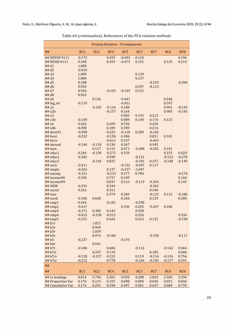
Peón, D., Martínez-Filgueira, X. M., & López-Iglesias, E. Revista Galega de Economía 2020, 29 (2), 6744
26
Table A4 (continuation). Robustness of the PCA rotation methods
Promax Rotation – 8 components
## RC1 RC2 RC4 RC5 RC3 RC7 RC6 RC8
## DEPOP.9111 -0.173 0.459 -0.403 0.118 0.196 ## RESID.9111 0.348 0.459 -0.473 0.191 0.125 0.214 ## d1 1.000 ## d2 -0.924 ## d3 1.009 0.139 ## d4 1.000 0.137 ## d5 0.188 -0.219 -0.398 ## d6 0.936 0.297 -0.113 ## d7 0.920 -0.145 -0.149 0.122 ## d8 0.963 ## x0 0.136 -0.441 0.546 ## log_x0 -0.119 -0.451 0.597 ## x2 -0.103 -0.116 0.180 0.901 -0.129 ## x2b -0.157 0.164 0.905 -0.145 ## x3 0.983 0.193 0.213 ## x3b -0.109 0.989 0.140 0.176 0.123 ## x4 0.442 0.209 0.726 0.224 ## x4b 0.398 0.189 0.789 0.214 ## dens91 -0.390 0.225 -0.118 0.209 -0.102 ## forei -0.232 -0.150 0.306 0.811 0.101 ## born -0.611 0.137 -0.463 ## abroad -0.146 -0.110 0.136 0.347 0.945 ## men 0.117 0.131 0.471 -0.208 -0.292 0.101 ## educ1 0.246 -0.130 -0.273 0.159 0.155 0.424 ## educ2 -0.302 0.590 -0.121 -0.123 -0.278 ## educ3 -0.146 0.825 -0.102 0.257 -0.148 -0.149 ## activ -0.411 -0.132 -0.997 0.117 ## emplo -0.264 0.137 -0.157 -1.047 ## unemp -0.151 -0.233 0.177 0.784 -0.174 ## income96 0.328 0.737 0.109 0.160 ## income09 0.847 0.116 -0.119 -0.354 0.145 ## ISDN -0.291 0.344 -0.365 ## social 0.263 0.311 0.340 ## tour 0.374 0.260 -0.133 0.112 -0.186 ## work -0.106 0.668 0.184 0.129 0.200 ## emp1 0.444 -0.181 -0.598 ## emp2 -0.417 0.396 0.255 -0.247 0.186 ## emp3 -0.171 0.386 0.143 0.358 ## emp4 -0.415 -0.130 -0.311 0.526 0.334 ## emp5 -0.251 0.424 0.413 0.125 -0.158 ## b1r 1.021 ## b2r 0.964 ## b3r 1.039 ## b4r 0.974 -0.106 -0.130 -0.117 ## b5 -0.237 0.170 ## b6r 0.941 ## b7r -0.186 0.686 -0.112 -0.142 0.564 ## b7ir 0.247 0.118 0.185 0.606 ## b7cr -0.128 -0.157 0.222 0.119 -0.116 -0.124 0.756 ## b7sr -0.212 0.778 -0.166 -0.103 -0.117 0.291
##
## RC1 RC2 RC4 RC5 RC3 RC7 RC6 RC8
## ss loadings 8.814 5.744 5.361 4.920 4.208 2.823 2.569 2.294 ## Proportion Var 0.176 0.115 0.107 0.098 0.084 0.056 0.051 0.046 ## Cumulative Var 0.176 0.291 0.398 0.497 0.581 0.637 0.689 0.735
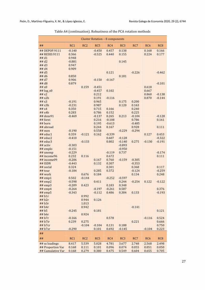
Peón, D., Martínez-Filgueira, X. M., & López-Iglesias, E. Revista Galega de Economía 2020, 29 (2), 6744
27
Table A4 (continuation). Robustness of the PCA rotation methods
Cluster Rotation – 8 components
## RC1 RC2 RC5 RC4 RC3 RC7 RC6 RC8
## DEPOP.9111 -0.140 -0.450 0.457 0.138 0.168 0.166 ## RESID.9111 0.366 -0.525 0.440 0.155 0.224 0.177 ## d1 0.948 ## d2 -0.881 0.145 ## d3 0.947 ## d4 0.909 ## d5 0.121 -0.226 -0.462 ## d6 0.850 0.181 ## d7 0.906 -0.150 -0.167 ## d8 0.879 -0.101 ## x0 0.159 -0.451 0.618 ## log_x0 -0.457 0.102 0.667 ## x2 0.212 0.860 -0.138 ## x2b 0.191 -0.116 0.870 -0.144 ## x3 -0.191 0.965 0.175 0.200 ## x3b -0.231 0.987 0.120 0.163 ## x4 0.350 0.715 0.166 0.240 ## x4b 0.283 0.786 0.152 0.225 ## dens91 -0.469 -0.137 0.265 0.213 -0.104 -0.128 ## forei 0.216 -0.108 0.786 0.161 ## born 0.195 -0.613 -0.485 ## abroad 0.244 0.167 0.928 0.111 ## men -0.190 0.558 -0.229 -0.294 ## educ1 0.359 -0.121 0.162 -0.339 0.127 0.453 ## educ2 -0.410 0.607 -0.128 -0.322 ## educ3 -0.133 0.802 -0.140 0.275 -0.130 -0.191 ## activ -0.303 -0.893 ## emplo -0.151 -0.950 ## unemp -0.229 -0.119 0.737 -0.174 ## income96 0.232 0.116 0.672 0.111 ## income09 -0.206 0.167 0.760 -0.159 -0.305 ## ISDN -0.443 0.132 0.307 -0.353 ## social 0.324 0.301 0.368 0.117 ## tour -0.184 0.285 0.372 -0.124 -0.259 ## work 0.676 0.184 0.134 0.248 ## emp1 0.502 -0.144 -0.252 -0.597 ## emp2 -0.598 0.411 0.244 -0.254 0.122 -0.122 ## emp3 -0.209 0.423 0.183 0.348 ## emp4 -0.264 -0.197 -0.261 0.587 0.376 ## emp5 -0.343 -0.112 0.486 0.384 0.133 -0.193 ## b1r 0.992 ## b2r 0.944 0.126 ## b3r 1.013 ## b4r 0.942 -0.141 ## b5 -0.245 0.181 0.121 ## b6r 0.924 ## b7r -0.166 0.578 -0.116 0.524 ## b7ir 0.239 0.275 0.221 0.666 ## b7cr -0.104 -0.104 0.131 0.188 0.750 ## b7sr -0.290 0.101 0.692 -0.145 -0.104 0.223
##
## RC1 RC2 RC5 RC4 RC3 RC7 RC6 RC8
## ss loadings 8.417 5.539 5.028 4.781 3.677 2.748 2.568 2.498 ## Proportion Var 0.168 0.111 0.101 0.096 0.074 0.055 0.051 0.050 ## Cumulative Var 0.168 0.279 0.380 0.475 0.549 0.604 0.655 0.705
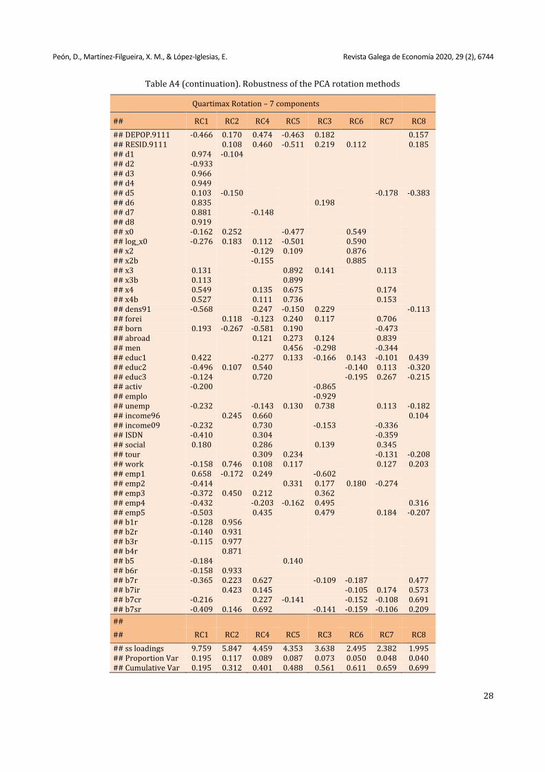
Peón, D., Martínez-Filgueira, X. M., & López-Iglesias, E. Revista Galega de Economía 2020, 29 (2), 6744
28
Table A4 (continuation). Robustness of the PCA rotation methods
Quartimax Rotation – 7 components
## RC1 RC2 RC4 RC5 RC3 RC6 RC7 RC8
## DEPOP.9111 -0.466 0.170 0.474 -0.463 0.182 0.157 ## RESID.9111 0.108 0.460 -0.511 0.219 0.112 0.185 ## d1 0.974 -0.104 ## d2 -0.933 ## d3 0.966 ## d4 0.949 ## d5 0.103 -0.150 -0.178 -0.383 ## d6 0.835 0.198 ## d7 0.881 -0.148 ## d8 0.919 ## x0 -0.162 0.252 -0.477 0.549 ## log_x0 -0.276 0.183 0.112 -0.501 0.590 ## x2 -0.129 0.109 0.876 ## x2b -0.155 0.885 ## x3 0.131 0.892 0.141 0.113 ## x3b 0.113 0.899 ## x4 0.549 0.135 0.675 0.174 ## x4b 0.527 0.111 0.736 0.153 ## dens91 -0.568 0.247 -0.150 0.229 -0.113 ## forei 0.118 -0.123 0.240 0.117 0.706 ## born 0.193 -0.267 -0.581 0.190 -0.473 ## abroad 0.121 0.273 0.124 0.839 ## men 0.456 -0.298 -0.344 ## educ1 0.422 -0.277 0.133 -0.166 0.143 -0.101 0.439 ## educ2 -0.496 0.107 0.540 -0.140 0.113 -0.320 ## educ3 -0.124 0.720 -0.195 0.267 -0.215 ## activ -0.200 -0.865 ## emplo -0.929 ## unemp -0.232 -0.143 0.130 0.738 0.113 -0.182 ## income96 0.245 0.660 0.104 ## income09 -0.232 0.730 -0.153 -0.336 ## ISDN -0.410 0.304 -0.359 ## social 0.180 0.286 0.139 0.345 ## tour 0.309 0.234 -0.131 -0.208 ## work -0.158 0.746 0.108 0.117 0.127 0.203 ## emp1 0.658 -0.172 0.249 -0.602 ## emp2 -0.414 0.331 0.177 0.180 -0.274 ## emp3 -0.372 0.450 0.212 0.362 ## emp4 -0.432 -0.203 -0.162 0.495 0.316 ## emp5 -0.503 0.435 0.479 0.184 -0.207 ## b1r -0.128 0.956 ## b2r -0.140 0.931 ## b3r -0.115 0.977 ## b4r 0.871 ## b5 -0.184 0.140 ## b6r -0.158 0.933 ## b7r -0.365 0.223 0.627 -0.109 -0.187 0.477 ## b7ir 0.423 0.145 -0.105 0.174 0.573 ## b7cr -0.216 0.227 -0.141 -0.152 -0.108 0.691 ## b7sr -0.409 0.146 0.692 -0.141 -0.159 -0.106 0.209
##
## RC1 RC2 RC4 RC5 RC3 RC6 RC7 RC8
## ss loadings 9.759 5.847 4.459 4.353 3.638 2.495 2.382 1.995 ## Proportion Var 0.195 0.117 0.089 0.087 0.073 0.050 0.048 0.040 ## Cumulative Var 0.195 0.312 0.401 0.488 0.561 0.611 0.659 0.699
Peón, D., Martínez-Filgueira, X. M., & López-Iglesias, E. Revista Galega de Economía 2020, 29 (2), 6744
29
References
Akgün, A. A., Baycan, T., & Nijkamp, P. (2015). Rethinking on sustainable rural development. European Planning Studies, 23(4), 678-692. DOI: https://doi.org/10.1080/09654313.2014.945813
Artz, G. M., Cho, I., Guo, Z., Kim, Y., Orazem, P. F., & Yu, L. (2015). Eighty years of research on rural economic development, agglomeration, migration, commuting, income, innovation, and entrepreneurship: The Iowa State human capital tradition. AgBioForum, 18(3), 243-251. Retrieved from: http://www.agbioforum.org/v18n3/v18n3a02-artz.htm
Barbut, L. (2009). L’évaluation ex post du PDRN: un regard instructif sur le passé pour améliorer l’avenir. Notes et Études Socio-Économiques, 33, 7-39. Retrieved from: http://37.235.92.116/IMG/pdf_nese091133A1.pdf
Bryden, J., & Munro, G. (2000). New approaches to economic development in peripheral rural regions. Scottish Geographical Journal, 116(2), 111-124. DOI: https://doi.org/10.1080/00369220018737085
Bureau, J. C. (2016). Workshop 1: Jobs, growth and investment in the wider rural economy. Cork 2.0 Conference on Rural Development, 5th Sept 2016, Cork, Ireland. Retrieved from: https://enrd.ec.europa.eu/cork-20-and-future-rural-development_en
Collantes, F., Pinilla, V., Sáez, L A., & Silvestre, J. (2014). Reducing depopulation in rural Spain: The impact of immigration. Population, Space and Place, 20(7), 606-621. DOI: https://doi.org/10.1002/psp.1797
Eguía, B., & Aldaz, L. (2019). Valoración de la vulnerabilidad demográfica y económica a escala local. El caso del País Vasco. Scripta Nova. Revista Electrónica de Geografía y Ciencias Sociales, XXIII(628). DOI: https://doi.org/10.1344/sn2019.23.22717
Eliasson, K., Westlund, H., & Johansson, M. (2015). Determinants of net migration to rural areas, and the impacts of migration on rural labour markets and self-employment in rural Sweden. European Planning Studies, 23(4), 693-709. DOI: https://doi.org/10.1080/09654313.2014.945814
Elshof, H., van Wissen, L., & Mulder, C. H. (2014). The self-reinforcing effects of population decline: An analysis of differences in moving behaviour between rural neighbourhoods with declining and stable populations. Journal of Rural Studies, 36, 285-299. DOI: https://doi.org/10.1016/j.jrurstud.2014.09.006
European Commission. (2013). Rural Development in the European Union. Statistical and Economic Information-Report 2013. Brussels, Belgium: European Commission. Directorate-General for Agriculture and Rural Development.
Eurostat. (2011) The degree of urbanization (DEGURBA). Luxembourg, Luxembourg: Eurostat. Retrieved from: http://ec.europa.eu/eurostat/ramon/miscellaneous/index.cfm?TargetUrl=DSP_DEGURBA
Fernández Leiceaga, X., & López Iglesias, E. (2000). Estrutura económica de Galiza. Santiago de Compostela: Laiovento.
Fernández, M., & Peón, D. (2017). Desafios dunha sociedade avellentada e en declive: desequilibrios territoriais e prestacion de servizos. Foro Económico de Galicia, Documento 20/2017.
Figueiredo, E. (2009). One rural, two visions: Environmental issues and images on rural areas in Portugal. Journal of European Countryside, 1(1), 9-21. DOI: https://doi.org/10.2478/v10091-009-0002-8
IGE. (2011). Clasificación do grao de urbanización das parroquias e concellos galegos (GU 2011). Santiago de Compostela: Instituto Galego de Estatística. Retrieved from: http://www.ige.eu/web/mostrar_paxina.jsp?paxina=003003001&idioma=gl
IGE. (2016). Clasificación das parroquias e concellos galegos segundo o grao de urbanización (GU 2016). Santiago de Compostela: Instituto Galego de Estatística. Retrieved from: http://www.ige.eu/web/mostrar_paxina.jsp?paxina=003003001&idioma=gl
Johnson, R. A., & Wichern, D. W. (2014). Applied multivariate statistical analysis, vol. 4. Englewood Cliffs, NJ: Prentice-Hall.
Li, M., Goetza, S. J., Partridge, M., & Fleming, D.A. (2016). Location determinants of high-growth firms. Entrepreneurship and Regional Development, 28(1–2), 97-125. DOI: https://doi.org/10.1080/08985626.2015.1109003
López Iglesias, E. (1995). Demografía e estruturas agrarias. Análise da dinámica demográfica e das mudanças nas estruturas fundiárias da agricultura galega, 1950-1993. Santiago de Compostela: Universidade de Santiago de Compostela.
López Iglesias, E. (2013). A gobernanza e xestión do medio rural galego a comezos do século XXI: Reflexións e propostas para o debate. In R. Rodríguez González (Coord.), Galicia, un mundo rural vivo (pp. 130-147). Lalín (Pontevedra): Universidad Internacional Menéndez Pelayo / Concello de Lalín. Retrieved from: https://lalin.gal/files/Galicia%20un%20mundo%20rural%20vivo%20baja.pdf
Peón, D., Martínez-Filgueira, X. M., & López-Iglesias, E. Revista Galega de Economía 2020, 29 (2), 6744
30
López Iglesias, E., Peón, D., & Rodríguez Álvarez, J. (2018). Mobility innovations for sustainability and cohesion of rural areas: A transport model and public investment analysis for Valdeorras (Galicia, Spain). Journal of Cleaner Production, 172, 3520-3534. DOI: https://doi.org/10.1016/j.jclepro.2017.05.149
Marsden, T., & Sonnino, R. (2008). Rural development and the regional state: Denying multifunctional agriculture in the UK. Journal of Rural Studies, 24, 422-431. DOI: https://doi.org/10.1016/j.jrurstud.2008.04.001
Martínez Filgueira, X., Peón, D., & López Iglesias, E. (2017). Intra-rural divides and regional planning within regions in demographic decline. Analysis of a traditional emigration region (Galicia, Spain). European Planning Studies, 25(7), 1237-1255. DOI: https://doi.org/10.1080/09654313.2017.1319465
Peón, D., & Martínez Filgueira, X. (2019). Determinants of investing in innovative activities by agri-food and KIBS firms in rural areas: An exploratory analysis. Journal of Small Business Management. DOI: https://doi.org/10.1111/jsbm.12513
Míguez Macho, L. (2013). Gobierno y gestión del medio rural en Galicia. La reforma de la administración local. In R. Rodríguez González (Coord.), Galicia, un mundo rural vivo (pp. 148-159). Lalín (Pontevedra): Universidad Internacional Menéndez Pelayo / Concello de Lalín. Retrieved from: https://lalin.gal/files/Galicia%20un%20mundo%20rural%20vivo%20baja.pdf
Phelan, C., & Sharpley, R. (2011). Exploring agritourism entrepreneurship in the UK. Tourism Planning & Development, 8(2), 121-136. DOI: https://doi.org/10.1080/21568316.2011.573912
Revelle, W. (2017). Psych: Procedures for personality and psychological research. Version = 1.75. Evanston, IL: Northwestern University. Retrieved from: https://CRAN.R-project.org/package=psych
Rizzo, A. (2016). Declining, transition and slow rural territories in southern Italy: Characterizing the intra-rural divides. European Planning Studies, 24(2), 231-253. DOI: https://doi.org/10.1080/09654313.2015.1079588
Salvati, L., & Carlucci, M. (2016). Patterns of sprawl: The socioeconomic and territorial profile of dispersed urban areas in Italy. Regional Studies, 50(8), 1346-1359. DOI: https://doi.org/10.1080/00343404.2015.1009435
Sánchez-Zamora, P., Gallardo-Cobos, R., & Ceña-Delgado, F. (2014). Rural areas face the economic crisis: Analyzing the determinants of successful territorial dynamics. Journal of Rural Studies, 35, 11-25. DOI: https://doi.org/10.1016/j.jrurstud.2014.03.007
Smailes, P. J., Argent, N., & Griffin, L.C. (2002). Rural population density: Its impact on social and demographic aspects of rural communities. Journal of Rural Studies, 18, 385-404. DOI: https://doi.org/10.1016/S0743-0167(02)00033-5
Spoor, M. (2013). Multidimensional social exclusion and the ‘rural-urban divide’ in Eastern Europe and Central Asia. Sociologia Ruralis, 53(2), 139-157. DOI: https://doi.org/10.1111/soru.12008
Stephens, H. M., Partridge, M. D., & Faggian, A. (2013). Innovation, entrepreneurship and economic growth in lagging regions. Journal of Regional Science, 53(5), 778-812. DOI: https://doi.org/10.1111/jors.12019
Xunta de Galicia. (2013). Plan para a dinamización demográfica de Galicia 2013-2016, Horizonte 2020. Santiago de Compostela: Xunta de Galicia. Consellería de Presidencia, AA.PP. e Xustiza. Retrieved from: http://www.xunta.es/c/document_library/get_file?folderId=577713&name=DLFE-19604.pdf
Xunta de Galicia. (2014). Diagnóstico de situación socioeconómica e territorial de Galicia para a elaboración dos POs FEDER e FSE Galicia 2014-2020. Santiago de Compostela: Xunta de Galicia. Consellería de Facenda. Dirección Xeral de Planificación e Orzamentos. Retrieved from: http://www.conselleriadefacenda.es/documents/10433/1347376/Diagnostico-Socioeconomico-Galicia-gal.pdf/a2b3ac61-d536-4058-9346-d3d0e18fb752