Embed Size (px)
Citation preview
Int. J. Appl. Comput. Math (2021) 7:69 https://doi.org/10.1007/s40819-021-00965-z
ORIG INAL PAPER
Production System in a Collaborative Supply ChainConsidering Deterioration
Jaime Acevedo-Chedid1 · Katherinne Salas-Navarro2 ·Holman Ospina-Mateus1 · Alina Villalobo1 · Shib Sankar Sana3
Accepted: 24 January 2021© The Author(s), under exclusive licence to Springer Nature India Private Limited part of Springer Nature 2021
AbstractThis research presents a mathematical model for a collaborative planning of the supply chaininvolving four echelons (supplier, production plants, distribution, retails, or clients). Themodel seeks to maximize profit (utility) when all members of the chain share informationrelated to demand. It is developed for the aggregate consolidation of different rawmaterials incement production. The novelty of the model is the consideration of products that deterioratein the process and thus it has effect on the production times in the plant and lead time. In thissupply chain, quality and compliant products and the return of deteriorated products are twoflows. The considerations are lead time, inventories with shortages and excesses, productiontimes in normal and extra days, and subcontracting, among others. A mixed integer linearprogramming with demand scenario analysis is used to optimize and analyze the uncertaintythat is consistent with the performance of the construction sector. The model is formedconsidering two suppliers, two production plants, two distributors, two retailers and two endcustomers. Four manufacturing inputs (raw materials) are considered for the manufactureof two types of products. A case study of the cement production supply chain of Cartagena(Colombia) is illustrated. The shared benefit is generated around 5 billion pesos (COP) forall members of the chain in a period of 6 months.
Keywords Collaborative supply chain · Deteriorating products · Reverse flow
B Shib Sankar [email protected]
Jaime [email protected]
Katherinne [email protected]
Holman [email protected]
Alina [email protected]
1 Department of Industrial Engineering, Universidad Tecnológica de Bolívar, Cartagena, Colombia
2 Department of Productivity and Innovation, Universidad de La Costa, Barranquilla, Colombia
3 Department of Mathematics, Kishore Bharati Bhagini Nivedita College, Behala, Kolkata 700060, India
0123456789().: V,-vol 123
69 Page 2 of 46 Int. J. Appl. Comput. Math (2021) 7:69
Introduction
The supply chain refers to the set of efficiently integrated companies that seek the beststrategies to deal with goods and products in a timely manner at the lowest cost, satisfyingthe requirements of consumers [14]. The supply chain process integrates organizations andcustomer–supplier relationships. An integrated, coordinated, and synchronized managementprovides effective solutions for decision-making in all actors in the chain. The optimalityof the supply chain allows profits in inventory, purchasing, transportation, information flow,customer service, and delivery times [2, 56].
The global dynamics of the economy and competitiveness require new challenges to inter-act and satisfy customers. Efficient analysis of the supply chain for the search for competitiveadvantages must consider all interactions and relationships among suppliers, manufactur-ers, distributors, and customers. A common goal shared by these actors in the chain is tomaximize profits and customer satisfaction which translates into greater profitability andcompetitiveness. Strategies such as cooperation and collaboration of the different actors gen-erate synergies and multiply the efforts of the logistics processes. Collaboration/cooperationin the supply chain guide processes to be more dynamic and competitive based on customerdemand, eliminating barriers in the network, and seeking to simplify and make activitiesmore efficiently.
This research seeks to develop a collaborative mathematical model in the supply chainfor production planning.Problems such as the loss of sales due to low or missing invento-ries, obsolescence and deterioration of products, high transportation, and inventory costs, anduncertainty in the demand informationmotivate the approach of thismathematicalmodel. Theproposedmodel considers a case study problem of a company in the mining sector to producecement in the city of Cartagena in Colombia. The productive chain of the Colombian min-ing sector deals with the exploration, exploitation, and commercialization of non-metallicminerals such as sand, limestones and clays, gypsum that are used to supply materials tocement or concrete in industrial production processes, housing construction and infrastruc-ture [47]. Hence the study of this chain is important in the social and economic developmentof Colombia [8]. The use of mathematical models becomes an essential tool for the designand implementation of supply chains [57]. Supply chain modeling helps to capture the com-plexity and integrate the resources andmathematical programming represents the best way toapproach the methodology for solving the problems of mining supply chains. Next, a literaryreview is developed in the field of collaboration/cooperation where mathematical modelingis applied in the supply chain.
Literature review
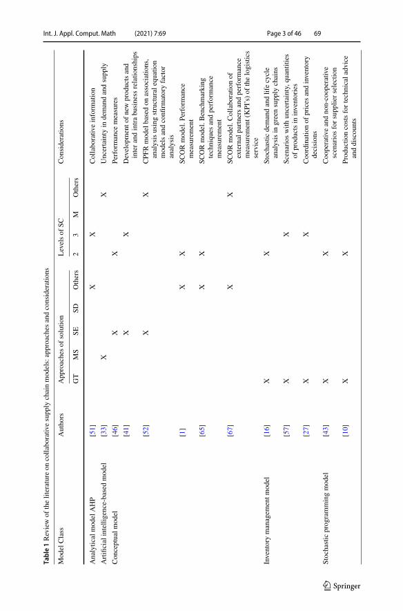
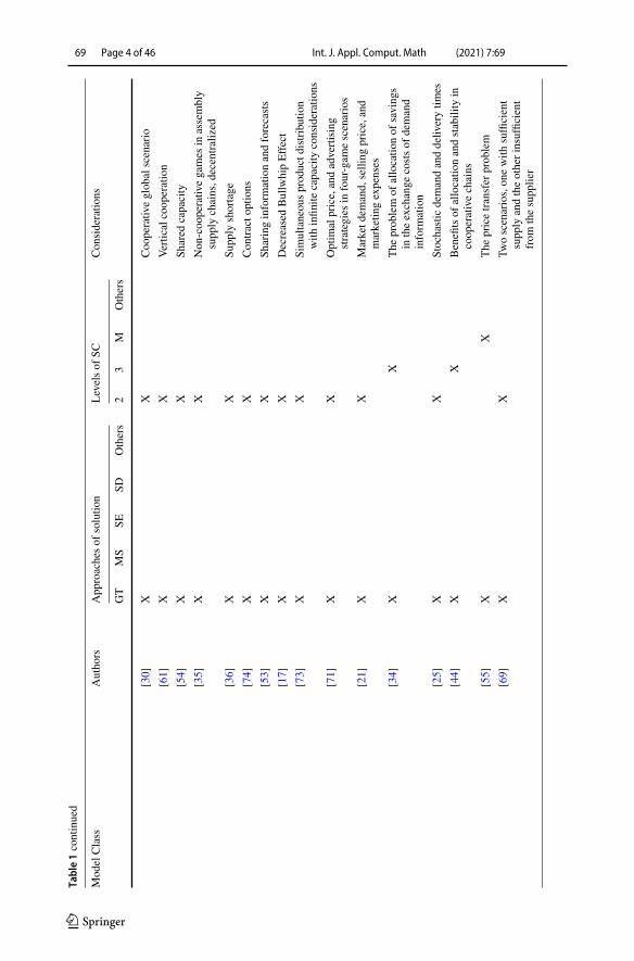
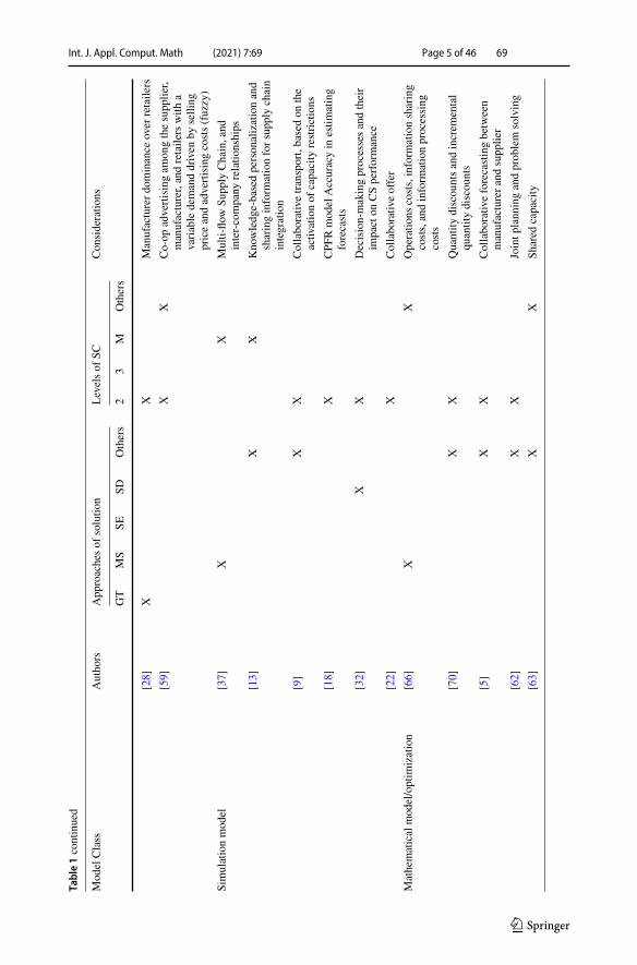
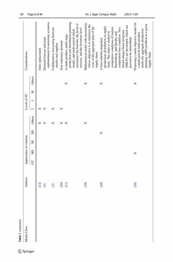
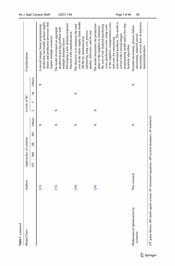
The concept of collaborative supply chains has taken on importance over the years [6, 19,23, 31, 38, 40, 62, 64]. The collaborative supply chain is characterized to integrate, relateto the long term, and define common targets and benefits [45, 57]. Joint efforts to achievethe same objective and economic benefits within the chain become a comprehensive solution[60]. Collaboration/cooperation avoid inefficiencies and the bullwhip effect produced by alack of coordination in the supply chain [26]. Table 1 shows the review of the literature oncollaborative supply chain models, based on the structure, approaches to the solution, andtheir characteristics.
In the literary review on models of collaboration/cooperation of logistics chains withdifferent approaches, no models are found that contemplate an integration in the supply
123
Int. J. Appl. Comput. Math (2021) 7:69 Page 3 of 46 69
Table1Reviewof
theliteratureon
colla
borativ
esupp
lychainmod
els:approaches
andconsiderations
Mod
elClass
Autho
rsApp
roachesof
solutio
nLevelsof
SCCon
sideratio
ns
GT
MS
SESD
Others
23
MOthers
AnalyticalmodelAHP
[51]
XX
Collabo
rativ
einform
ation
Artificialintelligence-basedmodel
[33]
XX
Uncertainty
indemandandsupp
ly
Con
ceptualm
odel
[46]
XX
Performance
measures
[41]
XX
Develop
mento
fnewprod
uctsand
interandintrabusiness
relatio
nships
[52]
XX
CPF
Rmodelbasedon
associations,
analysisusingstructuralequatio
nmod
elsandconfi
rmatoryfactor
analysis
[1]
XX
SCORmod
el.P
erform
ance
measurement
[65]
XX
SCORmod
el.B
enchmarking
techniqu
esandperformance
measurement
[67]
XX
SCORmod
el.C
ollabo
ratio
nof
externalpartnersandperformance
measurement(KPI’s)of
thelogistics
service
Inventorymanagem
entm
odel
[16]
XX
Stochasticdemandandlifecycle
analysisin
greensupply
chains
[57]
XX
Scenarioswith
uncertainty,quantities
ofprod
uctsin
inventories
[27]
XX
Coo
rdinationof
prices
andinventory
decision
s
Stochasticprog
rammingmod
el[43]
XX
Coo
perativ
eandno
n-coop
erative
scenariosforsupplierselection
[10]
XX
Productio
ncostsfortechnicaladvice
anddiscounts
123
69 Page 4 of 46 Int. J. Appl. Comput. Math (2021) 7:69
Table1continued
Mod
elClass
Autho
rsApp
roachesof
solutio
nLevelsof
SCCon
sideratio
ns
GT
MS
SESD
Others
23
MOthers
[30]
XX
Coo
perativ
eglob
alscenario
[61]
XX
Verticalcooperation
[54]
XX
Shared
capacity
[35]
XX
Non-cooperativ
egames
inassembly
supply
chains,d
ecentralized
[36]
XX
Supp
lyshortage
[74]
XX
Con
tracto
ptions
[53]
XX
Sharinginform
ationandforecasts
[17]
XX
Decreased
BullwhipEffect
[73]
XX
Simultaneou
sprod
uctd
istribution
with
infin
itecapacity
considerations
[71]
XX
Optim
alprice,andadvertising
strategies
infour-gam
escenarios
[21]
XX
Marketd
emand,
selling
price,and
marketin
gexpenses
[34]
XX
The
prob
lem
ofallocatio
nof
saving
sin
theexchange
costsof
demand
inform
ation
[25]
XX
Stochasticdemandanddeliv
erytim
es
[44]
XX
Benefitsof
allocatio
nandstability
incoop
erativechains
[55]
XX
The
pricetransfer
prob
lem
[69]
XX
Twoscenarios,onewith
sufficient
supp
lyandtheotherinsufficient
from
thesupp
lier
123
Int. J. Appl. Comput. Math (2021) 7:69 Page 5 of 46 69
Table1continued
Mod
elClass
Autho
rsApp
roachesof
solutio
nLevelsof
SCCon
sideratio
ns
GT
MS
SESD
Others
23
MOthers
[28]
XX
Manufacturerdo
minance
over
retaile
rs
[59]
XX
Co-op
advertisingam
ongthesupp
lier,
manufacturer,andretailerswith
avariabledemanddriven
byselling
priceandadvertisingcosts(fuzzy)
Simulationmodel
[37]
XX
Multi-flo
wSu
pply
Chain,and
inter-company
relatio
nships
[13]
XX
Knowledge-basedpersonalizationand
sharinginform
ationforsupp
lychain
integration
[9]
XX
Collaborativ
etransport,basedon
the
activ
ationof
capacity
restrictions
[18]
XCPF
RmodelAccuracyin
estim
ating
forecasts
[32]
XX
Decision-makingprocessesandtheir
impacton
CSperformance
[22]
XCollabo
rativ
eoffer
Mathematicalmodel/optim
ization
[66]
XX
Operatio
nscosts,inform
ationsharing
costs,andinform
ationprocessing
costs
[70]
XX
Quantity
discountsandincrem
ental
quantitydiscou
nts
[5]
XX
Collaborativ
eforecastingbetween
manufacturerandsupp
lier
[62]
XX
Jointp
lann
ingandprob
lem
solving
[63]
XX
Shared
capacity
123
69 Page 6 of 46 Int. J. Appl. Comput. Math (2021) 7:69
Table1continued
Mod
elClass
Autho
rsApp
roachesof
solutio
nLevelsof
SCCon
sideratio
ns
GT
MS
SESD
Others
23
MOthers
[12]
XX
Jointreplacement
[4]
XX
Dem
andforecastandjoint
replenishm
entinuncertainscenarios
[3]
XX
Collaborativ
eforecastingbetween
retailerandsupplier
[50]
XX
Non
-statio
nary
demand
[11]
XX
Amulti-prod
uct,multi-stage
prod
uctio
nanddistributio
nplanning
mod
el,and
multi-period
which
maxim
izes
thebenefits,thelevelo
fservices,and
theinventorylevel
[39]
XX
Mathematicalmodelwith
uncertainty,
whose
objectiveisto
minim
izethe
costsof
theaggregateplan
ofthe
supply
chain
[49]
XX
Afour-echelon
integrated
prod
uctio
n–distributio
nin
supp
lychain.
The
chainisstudiedin
competitivecond
ition
s(C
ournot,
Stackelberg,
andQualityand
competition-free
cond
ition
.Two
mixed-integer
linearprog
rams
(MILPs)aredeveloped,which
are
proved
tobe
unim
odular
[20]
XX
Prop
osingamulti-ob
jectivemod
elfor
amulti-period
multi-prod
uct
multi-siteaggregateprod
uctio
nplanning
(APP
)problem
inagreen
supply
chain
123
Int. J. Appl. Comput. Math (2021) 7:69 Page 7 of 46 69
Table1continued
Mod
elClass
Autho
rsApp
roachesof
solutio
nLevelsof
SCCon
sideratio
ns
GT
MS
SESD
Others
23
MOthers
[15]
XX
Amixed-integer
linearprog
ramming
mod
elthatcanhand
legeneralsup
ply
chains
andprod
uctio
nprocessesthat
requ
iremultip
leresources
[72]
XX
The
mod
eldevelopedan
aggregate
prod
uctio
n-pricingprob
lem
with
multip
ledemandclasses.
Develop
inganewdemandrespon
sefunctio
nwith
cannibalization
[58]
XX
The
objectiveisto
minim
izethetotal
costof
theentiresupp
lychainmod
el(SCM)by
simultaneously
optim
izingsetupcost,p
rocess
quality,d
eliveries,andlotsize
[24]
XX
The
mod
eldeterm
ines
theprod
uctio
nplansof
thesupp
liersto
minim
ize
thesum
ofrawmaterialp
urchasing
costs,productio
ncosts,setupcosts
ofthesuppliers,transportationcosts,
andcostsforou
tsou
rcing
semi-fin
ishedprod
ucts.T
hemod
elis
solved
with
amixed-integer
prog
rammingmod
elandatwo-step
heuristic
algorithm
Mathematicaloptim
izationby
scenarios
Thisresearch
XX
Dem
anduncertainty,processfailu
reuncertainty,materialarrival
uncertainty,reverseflo
wof
defective
materials/products
GTgametheory;M
Smulti-agentsystem;S
Estructuralequatio
ns;S
Dsystem
dynamics;M
multilevel
123
69 Page 8 of 46 Int. J. Appl. Comput. Math (2021) 7:69
chain of non-metallic minerals such as cement production. The proposed model helps to planthe production of final products, the distribution of materials, and integrates functions fromsuppliers to customers, synchronizing, and collaborating among all the actors in the chain.Additionally, the model considers uncertainty in demand, uncertain delays due to processfailures, and even uncertainty inmaterial quantities. Themodel contributes to planningwithinthe medium and short term at the tactical and operational levels of the supply chain.
The present research develops a collaborative supply chain planningmodelwhere themainobjective is to maximize the benefits of all the members in the four-echelon supply chaincomprising of suppliers, manufacturers, distributors, and retailers. The novelty of the modelallows considering a mechanism for detecting products with minor defects or deterioration.These products are purchased at a lower price, avoiding return, which favors less use oftransport and environmental impact. Additionally, it is considered a mechanism for detectingproducts with major defects in buyers (plants and distributors). The model considers returnsand changes in delivery times. Likewise, the lead time is considered at the supplier/producerand producer/distributor. The model considers production with work on regular and extradays, and subcontracting also.
The content of this research is structured as follows: The introduction in Sect. 1 indicatesthe context of the problem. The methods in Sect. 2 present the elements for mathematicalformulation. Sections 3 and 4 provide the case study and its results. Sections 5 and 6 providemanagerial implications and conclusions of the proposed model respectively.
Method
The proposed model is of a mixed-integer linear programming approach with analysis byscenarios for demand according to the economic performance of the construction sector. Themodel allows to plan the transport in each echelon, plan the purchases with the suppliers,plan the production of the plant, the sales, the inventory levels, and calculation of the totalcost. The chain integrates suppliers, production plants, distribution centers, retailers or cus-tomers.Suppliers deliver raw materials or items to the production plants, which transformthem into finished products. The distribution centers receive the products from the produc-tion plants and deliver them to the retailers, who sell the products to the final client. Thismodel maximizes the benefits of all members of the supply chain, considering parametersrelated to the production process, transport (times and capacities), inventories (capacities andshortage), and costs.
Fundamental Assumptions
The following assumptions are used to formulate the model:
The objective is to guarantee the maximization of the profit margin of all the entities ofthe supply chain (Revenues-Costs).Multiple suppliers, production plants, and multiple distribution centers are considered.Suppliers and production plants store raw material.There is a fraction of raw materials with deterioration/defect that can be purchased by theplants at a lower price.The lead times of plants and distribution centers are deterministic.There is a fraction of products with deterioration/defect that generate a non-rejectioncondition, which are bought by the next echelon at a lower price.
123
Int. J. Appl. Comput. Math (2021) 7:69 Page 9 of 46 69
At the beginning of each period new settings are given for production.Defective/deteriorated products purchased at plants from distributors are reprocessed andsold to the retailer as compliant products.Plants, distribution centers, and retailers store finished products.Three scenarios are proposed for the representation of the model under uncertainty, high,medium, and low scenario.
2.2. Notation
The following notations are used to develop the model.Declaration of Indices
s ∈ S: Suppliersp ∈ P: Plantsd ∈ D: Distribution Centersr ∈ R: Retailersc ∈ C : Clientst ∈ T : Periodse ∈ E : Scenariosm ∈ M : Raw Materialsj ∈ J : Productsq ∈ Q: Production Resources
Declaration of Sets
Sm : Set of suppliers s that provide raw material m (Sm ⊆ S)S p: Set of suppliers s that provide production plant p (S p ⊆ S)Qp: Set of production resources q of the plants p (Qp ⊆ Q)Dp: Set of distribution centers d that receive finished products j (Dp ⊆ D)Rd : Set of retailers r that receive finished products from distribution centers d (Rd ⊆ R)Cr : Set of clients that receive finished products from retailers r (Cr ⊆ C Jq .Jq : Set of finished products j produced with the production resource q (Jq ⊆ J )Jm : Set of finished products j produced with the raw material m (Jm ⊆ J ).
2.3. Statement of Parameters
Suppliers’ Parameters
CCSs,m,t : Cost per unit of raw material, component, or item m at supplier s in period t
($/Ton)HSs,m : Handling cost per unit at supplier s for the raw material m ($/Ton)
π+s,m : Inventory excess cost at supplier s for the raw material m ($/Ton)
π−s,m : Inventory shortage cost at supplier s for the raw material m ($/Ton)
CPSs,m,t : Production cost per unit at supplier s for the raw material m in period t($/Ton)
CDSs,m : Disposal cost per unit defective item at supplier s for raw material m ($/Ton)
CFT Ss,p,m : Fixed transportation cost at supplier s for the rawmaterialm for the production
plant p($)CT S
s,p,m : Transportation cost per unit from the supplier s to production plant p for the rawmaterial m ($/Ton)
123
69 Page 10 of 46 Int. J. Appl. Comput. Math (2021) 7:69
CT 1Sp,s,m : Transportation cost per unit from the production plant p to supplier s for theraw material m ($/Ton)αSs,m : Expected percentage of defective items at supplier s for the raw material m(0 ≤ αS
s,m ≤ 1)
βSs,m : Screening rate (%) of defective items at supplier s for the raw material m
CapT Ss,p,m : Transport capacity for the rawmaterialm from the supplier s to the production
plant p (Ton)T T S
s,p: Transportation time from supplier s to production plant p (Hours)
I oSs,m : Initial inventory level at supplier s for the raw material m (Ton)ImaxSs : Maximum inventory capacity at the supplier s (Ton)FmaxSs,m : Maximum production capacity at the supplier s for the raw material m (Ton)PV S
s,p,m : Selling price of raw material, component, or item m at the production plant p($/Ton)PV DS
s,p,m : Selling price per unit defective item at supplier s for the raw material m forthe production plant p ($/Ton)
Production Plants’ Parameters
CFPp,q, j,t : Fixed cost of changing material at plant p with the production resource q for
the finished product j in period t ($)CPRP
p,q, j,t : Production cost per unit at production plant p for the finished product jworking in regular time with the production resource q in period t ($/Ton)CPEP
p,q, j,t : Production cost per unit at production plant p for the finished product jworking in extra time with the production resource q in period t ($/Ton)CSubPp, j : Purchasing cost per unit subcontracted in the production plant p for the finishedproduct j ($/Ton)ϕp,q, j,t : Fixed handling cost at production plant p for the finished product j with theproduction resource q in period t($)HP
p, j : Handling cost per unit at production plant p for the finished product j ($/Ton)ϕ+p, j : Inventory excess cost at production plant p for the finished product j ($/Ton)
ϕ−p, j : Inventory shortage cost at production plant p for the finished product j ($/Sack)
CFT Pp,d, j : Fixed transportation cost for finished product j from production plant p to
distribution center d ($)CT P
p,d, j : Transportation cost per unit for finished product j from production plant p todistribution center d ($/Ton)MAP
m, j : Combination of rawmaterialm necessary to produce the finished product j (Sack)
CDPp, j : Disposal cost per unit defective item at production plan p for the finished product
j ($/Sack)βPp,m : Screening rate (%) of defective items at production plant p for the raw material m.
αPp, j : Expected percentage of defective items at production plant p for the finished product
j(0 ≤ αP
p, j ≤ 1)
μPp, j : Screening rate (%) of defective items at production plant p for the finished product
jCapPRP
p,q,t : Maximum production capacity at production plant pworking in regular timeon the production resource q in period t (Sacks)CapPEP
p,q,t : Maximum production capacity at production plant p working in extra timeon the production resource q in period t (Ton)
123
Int. J. Appl. Comput. Math (2021) 7:69 Page 11 of 46 69
CapT I Pp : Maximum capacity of transport input in the plant p (Ton)
CapT OPp : Maximum capacity of transport output in the plant p. (Sacks)
CapT Pp,d, j : Transport capacity for finished product j from production plant p to distribu-
tion center d (Ton)T T P
p,d : Transportation time from the production plant p to the distribution center d (Hours)
I oPp, j : Initial inventory level at production plant p for the finished product j (Ton)
Imax Pp : Maximum inventory capacity at the production plant p (Ton)
xpected percentage (%) of finished product j for subcontracting in the production plant p.PV P
p,d, j : Selling price per unit good item at production plant p to distrsibution center dfor the finished product j ($/Ton)PV DP
p,d, j : Selling price per unit defective item at production plant p to distribution centerd for the finished product j ($/Ton)
Distribution Centers’ Parameters
HDd, j : Handling cost per unit at the distribution center d for the finished product j ($/Sack)
γ +d, j : Excess inventory cost at distribution center d for the finished product j ($/Sack)
γ −d, j : Shortage inventory cost at distribution center d for the finished product j ($/Sack)
CFT Dd,r , j : Fixed transportation cost from distribution center d to the retailer r for the
finished product j($)CT D
d,r , j : Fixed transportation cost per unit from distribution center d to the retailer r forthe finished product j ($/Sack)CDD
d, j : Disposal cost per unit defective item at distribution center d for the finished productj ($/Sack)δDd, j : Screening-rate (%) of defective items at distribution center d for the finished productj .CapT OD
d : Maximum capacity of transport output in the distribution center d (Sacks)CapT D
d,r , j : Transportation capacity of finished product j from distribution center d to theretailer r (Sacks)T T D
d,r : Transportation time from the distribution center d to the retailer r (Hours)
I oDd, j : Initial inventory level at distribution center d for the finished product j (Sacks)
ImaxDd : Maximum inventory capacity at distribution center d (Sacks)PV D
d,r , j : Selling price per unit good item at distribution center d to the retailer r for thefinished product j ($/Sack)
Retailers’ Parameters.
HRr , j : Handling cost per unit at retailer r for the finished product j ($/Sack)
ϑ+r , j : Excess inventory cost at retailer r for the finished product j ($/Sack)
ϑ−r , j : Shortage inventory cost at retailer r for the finished product j ($/Sack)
I oRr , j : Initial inventory level at retailer r for the finished product j (Sacks)
Imax Rr : Maximum inventory capacity at retailer r (Sacks)CapT OR
r : Maximum capacity of transport input in the retailer r (Sacks)DemC
c, j,t,e: Demand rate of client c for the finished product j over scenario e in period t(Sacks)PV R
r ,c, j : Selling price per unit good item at retailer r to the client c for the finished productj ($/Sack)Probe: Probability over scenario e.
123
69 Page 12 of 46 Int. J. Appl. Comput. Math (2021) 7:69
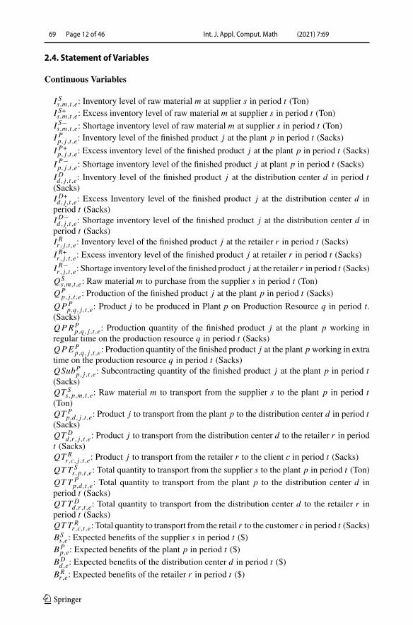
2.4. Statement of Variables
Continuous Variables
I Ss,m,t,e: Inventory level of raw material m at supplier s in period t (Ton)I S+s,m,t,e: Excess inventory level of raw material m at supplier s in period t (Ton)
I S−s,m,t,e: Shortage inventory level of raw material m at supplier s in period t (Ton)I Pp, j,t,e: Inventory level of the finished product j at the plant p in period t (Sacks)
I P+p, j,t,e: Excess inventory level of the finished product j at the plant p in period t (Sacks)
I P−p, j,t,e: Shortage inventory level of the finished product j at plant p in period t (Sacks)
I Dd, j,t,e: Inventory level of the finished product j at the distribution center d in period t(Sacks)I D+d, j,t,e: Excess Inventory level of the finished product j at the distribution center d inperiod t (Sacks)I D−d, j,t,e: Shortage inventory level of the finished product j at the distribution center d inperiod t (Sacks)I Rr , j,t,e: Inventory level of the finished product j at the retailer r in period t (Sacks)
I R+r , j,t,e: Excess inventory level of the finished product j at retailer r in period t (Sacks)
I R−r , j,t,e: Shortage inventory level of the finished product j at the retailer r in period t (Sacks)
QSs,m,t,e: Raw material m to purchase from the supplier s in period t (Ton)
QPp, j,t,e: Production of the finished product j at the plant p in period t (Sacks)
QPPp,q, j,t,e: Product j to be produced in Plant p on Production Resource q in period t.
(Sacks)QPRP
p,q, j,t,e: Production quantity of the finished product j at the plant p working inregular time on the production resource q in period t (Sacks)QPEP
p,q, j,t,e: Production quantity of the finished product j at the plant p working in extratime on the production resource q in period t (Sacks)QSubPp, j,t,e: Subcontracting quantity of the finished product j at the plant p in period t(Sacks)QT S
s,p,m,t,e: Raw material m to transport from the supplier s to the plant p in period t(Ton)QT P
p,d, j,t,e: Product j to transport from the plant p to the distribution center d in period t(Sacks)QT D
d,r , j,t,e: Product j to transport from the distribution center d to the retailer r in periodt (Sacks)QT R
r ,c, j,t,e: Product j to transport from the retailer r to the client c in period t (Sacks)
QTT Ss,p,t,e: Total quantity to transport from the supplier s to the plant p in period t (Ton)
QTT Pp,d,t,e: Total quantity to transport from the plant p to the distribution center d in
period t (Sacks)QTT D
d,r ,t,e: Total quantity to transport from the distribution center d to the retailer r inperiod t (Sacks)QTT R
r ,c,t,e: Total quantity to transport from the retail r to the customer c in period t (Sacks)BSs,e: Expected benefits of the supplier s in period t ($)
BPp,e: Expected benefits of the plant p in period t ($)
BDd,e: Expected benefits of the distribution center d in period t ($)
BRr ,e: Expected benefits of the retailer r in period t ($)
123
Int. J. Appl. Comput. Math (2021) 7:69 Page 13 of 46 69
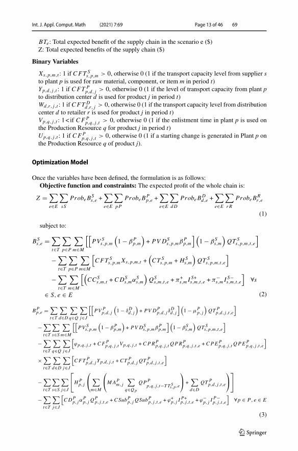
BTe: Total expected benefit of the supply chain in the scenario e ($)Z: Total expected benefits of the supply chain ($)
Binary Variables
Xs,p,m,t : 1 if CFT Ss,p,m > 0, otherwise 0 (1 if the transport capacity level from supplier s
to plant p is used for raw material, component, or item m in period t)Yp,d, j,t : 1 if CFT P
p,d, j > 0, otherwise 0 (1 if the level of transport capacity from plant pto distribution center d is used for product j in period t)Wd,r , j,t : 1 if CFT D
d,r , j > 0, otherwise 0 (1 if the transport capacity level from distributioncenter d to retailer r is used for product j in period t)Vp,q, j,t : 1< if CFP
p,q, j,t > 0, otherwise 0 (1 if the enlistment time in plant p is used onthe Production Resource q for product j in period t)Up,q, j,t : 1 if CFP
p,q, j,t > 0, otherwise 0 (1 if a starting change is generated in Plant p onthe Production Resource q of product j).
OptimizationModel
Once the variables have been defined, the formulation is as follows:Objective function and constraints: The expected profit of the whole chain is:
Z �∑
e∈E
∑
sS
ProbeBSs,e +
∑
e∈E
∑
pP
ProbeBPp,e +
∑
e∈E
∑
dD
ProbeBDd,e +
∑
e∈E
∑
r R
ProbeBRr ,e
(1)
subject to:
(2)
BSs,e �
∑
t∈T
∑
p∈P
∑
m∈M
[[PV S
s,p,m
(1 − βP
p,m
)+ PV DS
s,p,mβPp,m
] (1 − βS
s,m
)QT S
s,p,m,t,e
]
−∑
t∈T
∑
p∈P
∑
m∈M
[CFT S
s,p,mXs,p,m,t +(CT S
s,p,m + HSs,m
)QT S
s,p,m,t,e
]
−∑
t∈T
∑
m∈M
[(CCS
s,m,t + CDSs,mαS
s,m
)QS
s,m,t,e + π+s,m I
S+s,m,t,e + π−
s,m IS−s,m,t,e
]∀s
∈ S, e ∈ E
BPp,e �
∑
t∈T
∑
d∈D
∑
q∈Q
∑
j∈J
[[PV P
p,d, j
(1 − δDd, j
)+ PV DP
p,d, j δDd, j
] (1 − μP
p, j
)QT P
p,d, j,t,e
]
−∑
t∈T
∑
s∈S
∑
m∈M
[[PV S
s,p,m
(1 − βP
p,m
)+ PV DS
s,p,mβPp,m
] (1 − βS
s,m
)QT S
s,p,m,t,e
]
−∑
t∈T
∑
q∈Q
∑
j∈J
[ϕp,q, j ,t + CFP
p,q, j ,t Vp,q, j ,t + CPRPp,q, j ,t QPRP
p,q, j,t,e + CPEPp,q, j,t QPE P
p,q, j,t,e
]
×∑
t∈T
∑
d∈D
∑
j∈J
[CFT P
p,d, j Yp,d, j ,t + CT Pp,d, j QT P
p,d, j ,t,e
]
−∑
t∈T
∑
s∈S
∑
j∈J
⎡
⎣HPp, j
⎛
⎝∑
m∈M
⎛
⎝MAPm, j
∑
q∈Qp
QPPp,q, j ,t−T T S
s,p ,e
⎞
⎠ +∑
d∈DQT P
p,d, j,t,e
⎞
⎠
⎤
⎦
−∑
t∈T
∑
j∈J
[CDP
p, jαPp, j Q
Pp, j ,t,e + CSubPp, j QSubPp, j ,t,e + ϕ+p, j I
P+p, j,t,e + ϕ−
p, j IP−p, j,t,e
]∀p ∈ P, e ∈ E
(3)
123
69 Page 14 of 46 Int. J. Appl. Comput. Math (2021) 7:69
BDd,e �
∑
t∈T
∑
r∈R
∑
j∈J
(PV D
d,r , j QT Dd,r , j,t,e
)
−∑
t∈T
∑
p∈P
∑
j∈J
[[PV P
p,d, j
(1 − δDd, j
)+ PV DP
p,d, jβPp,mδDd, j
]
(1 − μP
p, j
)QT P
p,d, j,t,e + CDDd, j δ
Dd, j QT PDdpjt
]
−∑
t∈T
∑
d∈D
∑
j∈J
[CFT D
d,r , j Wd,r , j,t + CT Dd,r , j QT D
d,r , j,t,e
]
−∑
t∈T
∑
j∈J
⎡
⎣HDd, j
⎛
⎝∑
p∈P
QT pp,d, j,t−T T P
p,d,e+
∑
r∈R
QT Dd,r , j,t,e
⎞
⎠ + γ +d, j I
D+d, j,t,e + γ −
d, j ID−d, j,t,e
⎤
⎦ ∀d
∈ D, e ∈ E
(4)
(5)
BRr ,e �
∑
t∈T
∑
c∈C
∑
j∈J
(PV R
r ,c, j QT Rr ,c, j,t,e
)−
∑
t∈T
∑
d∈D
∑
j∈J
[PV D
d,r , j QT Dd,r , j,t,e
]
−∑
t∈T
∑
j∈J
[
HRr , j
(∑
d∈DQT D
d,r , j,t−T T Dd,r,e
+∑
r∈R
QT Rr ,c, j,t,e
)]
−∑
t∈T
∑
j∈J
[ϑ+r , j I
R+r , j,t,e + ϑ−
r , j IR−r , j,t,e
]∀r ∈ R, e ∈ E
QPPp,q, j,t,e � QPRP
p,q, j,t,e + QPEPp,q, j,t,e ∀p ∈ P, q ∈ Q, j ∈ J , t ∈ T , e ∈ E (6)
CapPRPp,q,t kk ∀p ∈ P, q ∈ Q, t ∈ T , e ∈ E (7)
∑
j∈J
QPEPp,q, j,t,e ≤ CapPEP
p,q,t ∀p ∈ P, q ∈ Q, t ∈ T , e ∈ E (8)
∑
q∈Q
∑
j∈JqVp,q, j,t � 1 ∀p ∈ P, t ∈ T (9)
Up,q, j,t ≥ Vp,q, j,t − Vp,q, j,t−1 ∀p ∈ P, q ∈ Q, j ∈ J , t ∈ T (10)
QSubPp, j,t,e ≤ SubPp, j QPp, j,t,e ∀p ∈ P, j ∈ J , t ∈ T , e ∈ E (11)
(12)
QT Ss,p,m,t,e �
∑
j∈Jm
⎛
⎝MAPm, j
∑
q∈Qp
QPPp,q, j,t−T T S
s,p,e
⎞
⎠ ∀s
∈ S, p ∈ P,m ∈ M, t ∈ T , e ∈ E
QT Ss,p,m,t,e ≤ CapT S
s,p,mXs,p,m,t ∀s ∈ S, p ∈ P,m ∈ M, t ∈ T , e ∈ E (13)
QT Pp,d, j,t,e ≤ CapT P
p,d, j Yp,d, j,t ∀p ∈ P, d ∈ D, j ∈ J , t ∈ T , e ∈ E (14)
QT Dd,r , j,t,e ≤ CapT D
d,r , jWd,r , j,t ∀d ∈ D, r ∈ R, j ∈ J , t ∈ T , e ∈ E (15)
QT Rr ,c, j,t,e ≤ DemC
c, j,t,e ∀r ∈ R, c ∈ C, j ∈ J , t ∈ T , e ∈ E (16)
QTT Ss,p,t,e �
∑
m∈MQT S
s,p,m,t,e ∀s ∈ S, p ∈ P, t ∈ T , e ∈ E (17)
123
Int. J. Appl. Comput. Math (2021) 7:69 Page 15 of 46 69
QTT Pp,d,t,e �
∑
j∈J
QT Pp,d, j,t,e ∀p ∈ P, d ∈ D, t ∈ T , e ∈ E (18)
QTT Dd,r ,t,e �
∑
j∈J
QT Dd,r , j,t,e ∀d ∈ D, r ∈ R, t ∈ T , e ∈ E (19)
QTT Rr ,c,t,e �
∑
j∈J
QT Rr ,c, j,t,e ∀r ∈ R, c ∈ C, t ∈ T , e ∈ E (20)
∑
s∈S p
QT T Ss,p,t,e ≤ CapT I Pp ∀p ∈ P, t ∈ T , e ∈ E (21)
∑
d∈Dp
QT T Pp,d,t,e ≤ CapT OP
p ∀p ∈ P, t ∈ T , e ∈ E (22)∑
r∈Rp
QT T Dd,r ,t,e ≤ CapT OD
d ∀d ∈ D, t ∈ T , e ∈ E (23)∑
c∈C p
QT T Rr ,c,t,e ≤ CapT OR
r ∀r ∈ R, t ∈ T , e ∈ E (24)
I Ss,m,t,e � I Ss,m,t−1,e +(1 − αS
s,m
)QS
s,m,t,e −∑
p∈P
QT Ss,p,m,t,e ∀s ∈ S,m ∈ M, t ∈ T , e ∈ E (25)
I Pp, j,t,e � I Pp, j,t−1,e +(1 − αP
p, j
)QP
p, j,t,e −∑
d∈DQT P
p,d, j,t,e ∀p ∈ P, j ∈ J , t ∈ T , e ∈ E (26)
I Dd, j,t,e � I Dd, j,t−1,e +∑
p∈P
QDDp,d, j,t−T T P
p,d ,e−
∑
r∈R
QT Dd,r , j,t,e ∀d ∈ D, j ∈ J , t ∈ T , e ∈ E
(27)I Rr , j,t,e � I Rr , j,t−1,e +
∑
d∈DQRR
d,r , j,t−T T Dd,r ,e
−∑
c∈CQT R
r ,c, j,t,e ∀r ∈ R, j ∈ J , t ∈ T , e ∈ E (28)∑
m∈MI Ss,m,t,e ≤ ImaxSs ∀s ∈ S, t ∈ T , e ∈ E (29)
∑
j∈J
I Pp, j,t,e ≤ Imax Pp ∀p ∈ P, t ∈ T , e ∈ E (30)
∑
j∈J
I Dd, j,t,e ≤ ImaxDd ∀d ∈ D, t ∈ T , e ∈ E (31)
∑
j∈J
I Rr , j,t,e ≤ Imax Rr ∀r ∈ R, t ∈ T , e ∈ E (32)
I Ss,m,t,e � I S+s,m,t,e − I S−s,m,t,e ∀s ∈ S,m ∈ M, t ∈ T , e ∈ E (33)
I Pp, j,t,e � I P+p, j,t,e − I P−p, j,t,e ∀p ∈ P, j ∈ J , t ∈ T , e ∈ E (34)
I Dd, j,t,e � I D+d, j,t,e − I D−
d, j,t,e ∀d ∈ D, j ∈ J , t ∈ T , e ∈ E (35)
I Rr , j,t,e � I R+r , j,t,e − I R−r , j,t,e ∀r ∈ R, j ∈ J , t ∈ T , e ∈ E (36)
The variables (QSs,m,t,e, Q
Pp, j,t,e, QPP
p,q, j,t,e, QPRPp,q, j,t,e, QPEP
p,q, j,t,e, QSubPp, j,t,e,
QT Ss,p,m,t,e, QT P
p,d, j,t,e, QT Dd,r , j,t,e, QT R
r ,c, j,t,e, QTT Ss,p,t,e, QTT P
p,d,t,e, QTT Dd,r ,t,e,
QTT Rr ,c,t,e„ I S+s,m,t,e, I
S−s,m,t,e, I
P+p, j,t,e, I
P−p, j,t,e, I
D+d, j,t,e, I
D−d, j,t,e, I
R+r , j,t,e, I
R−r , j,t,e) are nonneg-
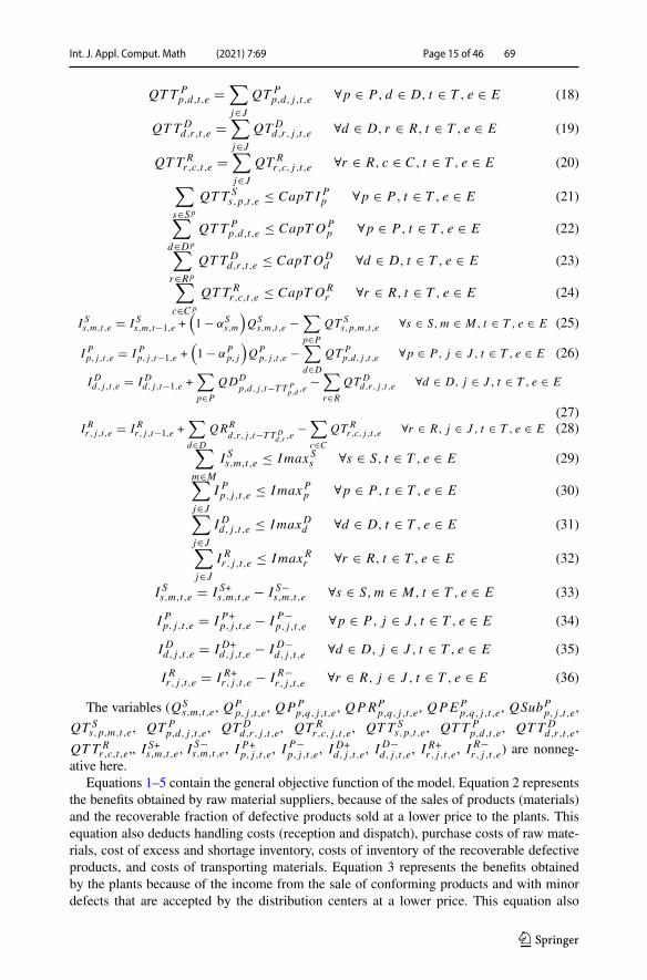
ative here.Equations 1–5 contain the general objective function of the model. Equation 2 represents
the benefits obtained by raw material suppliers, because of the sales of products (materials)and the recoverable fraction of defective products sold at a lower price to the plants. Thisequation also deducts handling costs (reception and dispatch), purchase costs of raw mate-rials, cost of excess and shortage inventory, costs of inventory of the recoverable defectiveproducts, and costs of transporting materials. Equation 3 represents the benefits obtainedby the plants because of the income from the sale of conforming products and with minordefects that are accepted by the distribution centers at a lower price. This equation also
123
69 Page 16 of 46 Int. J. Appl. Comput. Math (2021) 7:69
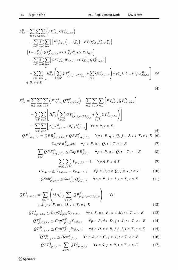
deducts fixed manufacturing costs, material handling costs, total manufacturing costs (nor-mal and overtime), subcontracting costs, material reception and dispatch costs, raw materialpurchase costs, cost of excess and shortage inventory, including the costs of defective productinventory and the cost of transportation.
Equation 4 represents the benefits obtained by the distribution centers because of theincome from the sale of products to retailers, deducting the costs of receipt and dispatch,the total cost of purchases from the plants, cost of excess and shortage inventory, defectiveproduct inventory costs, and transportation costs. Equation 5 represents the benefits obtainedby retailers because of the income from the sale of products to customers, deducting thecosts of receipt and dispatch, the total cost of purchases from the plants, cost of excess andshortage inventory, including the inventory of defective products detected and transportationcosts.
Equation 6 represents the amount of total production considering regular hours and over-time products. Equations 7 and 8 denote the maximum production capacity available duringregular working hours and overtime. Equations 9 and 10 specify that the manufacturing plantprepares for production or a possible change in a period. Equation 11 specifies the maximumamount of outsourcing. Equations 12–16 specify the quantity to be produced in a period.
Equations 17–20 specify the total quantities transported for each product in a period. Equa-tion 21 specifies the maximum inbound transportation capacity to the plant from suppliers.Equations 22–24 specify the maximum outbound transportation capacity from the plant tothe distribution center and from the distribution center to the retailer, and from the retailer tothe customer, respectively. Equations 25–28 correspond to the inventory balance equations ateach stage of the supply chain. Equations 29–32 represent the maximum inventory capacityin each of the stages of the chain. Equations 33–36 regulate the level of total inventory as theoccurrence of excess inventory or shortage inventory at each stage of the supply chain.
Case Study
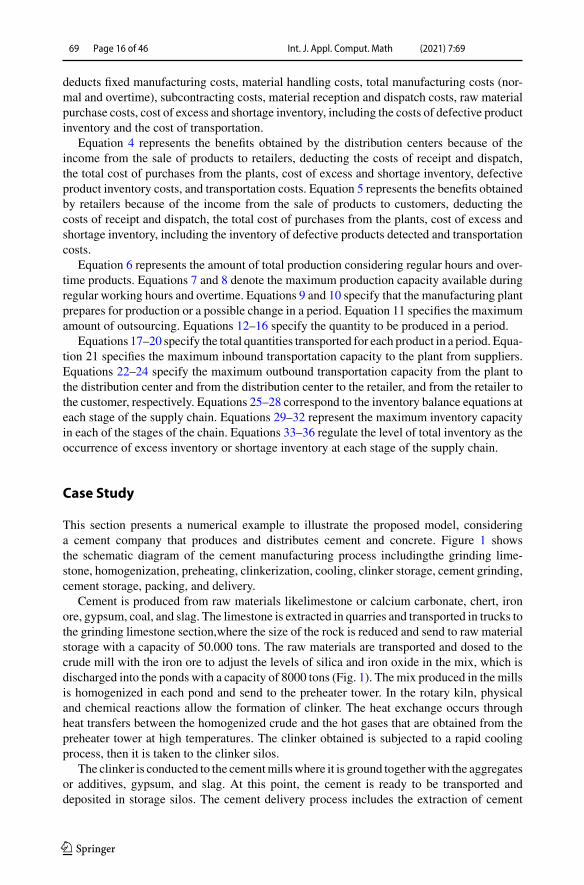
This section presents a numerical example to illustrate the proposed model, consideringa cement company that produces and distributes cement and concrete. Figure 1 showsthe schematic diagram of the cement manufacturing process includingthe grinding lime-stone, homogenization, preheating, clinkerization, cooling, clinker storage, cement grinding,cement storage, packing, and delivery.
Cement is produced from raw materials likelimestone or calcium carbonate, chert, ironore, gypsum, coal, and slag. The limestone is extracted in quarries and transported in trucks tothe grinding limestone section,where the size of the rock is reduced and send to raw materialstorage with a capacity of 50.000 tons. The raw materials are transported and dosed to thecrude mill with the iron ore to adjust the levels of silica and iron oxide in the mix, which isdischarged into the ponds with a capacity of 8000 tons (Fig. 1). The mix produced in the millsis homogenized in each pond and send to the preheater tower. In the rotary kiln, physicaland chemical reactions allow the formation of clinker. The heat exchange occurs throughheat transfers between the homogenized crude and the hot gases that are obtained from thepreheater tower at high temperatures. The clinker obtained is subjected to a rapid coolingprocess, then it is taken to the clinker silos.
The clinker is conducted to the cementmillswhere it is ground togetherwith the aggregatesor additives, gypsum, and slag. At this point, the cement is ready to be transported anddeposited in storage silos. The cement delivery process includes the extraction of cement
123
Int. J. Appl. Comput. Math (2021) 7:69 Page 17 of 46 69
Fig. 1 Benefits of the supply chain per month. (echelons vs. Profit ($COP Million))
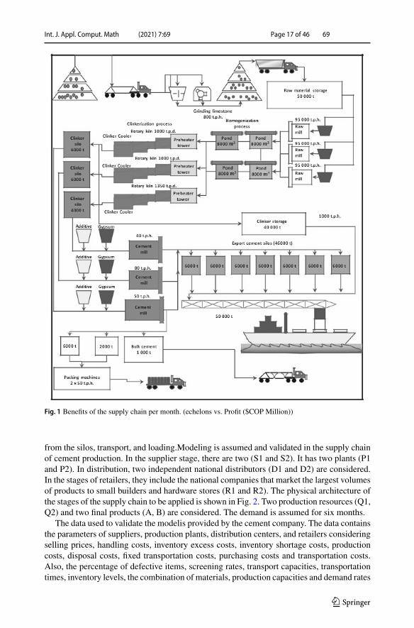
from the silos, transport, and loading.Modeling is assumed and validated in the supply chainof cement production. In the supplier stage, there are two (S1 and S2). It has two plants (P1and P2). In distribution, two independent national distributors (D1 and D2) are considered.In the stages of retailers, they include the national companies that market the largest volumesof products to small builders and hardware stores (R1 and R2). The physical architecture ofthe stages of the supply chain to be applied is shown in Fig. 2. Two production resources (Q1,Q2) and two final products (A, B) are considered. The demand is assumed for six months.
The data used to validate the modelis provided by the cement company. The data containsthe parameters of suppliers, production plants, distribution centers, and retailers consideringselling prices, handling costs, inventory excess costs, inventory shortage costs, productioncosts, disposal costs, fixed transportation costs, purchasing costs and transportation costs.Also, the percentage of defective items, screening rates, transport capacities, transportationtimes, inventory levels, the combination of materials, production capacities and demand rates
123
69 Page 18 of 46 Int. J. Appl. Comput. Math (2021) 7:69
Fig. 2 Physical architecture of the stages of the supply chain
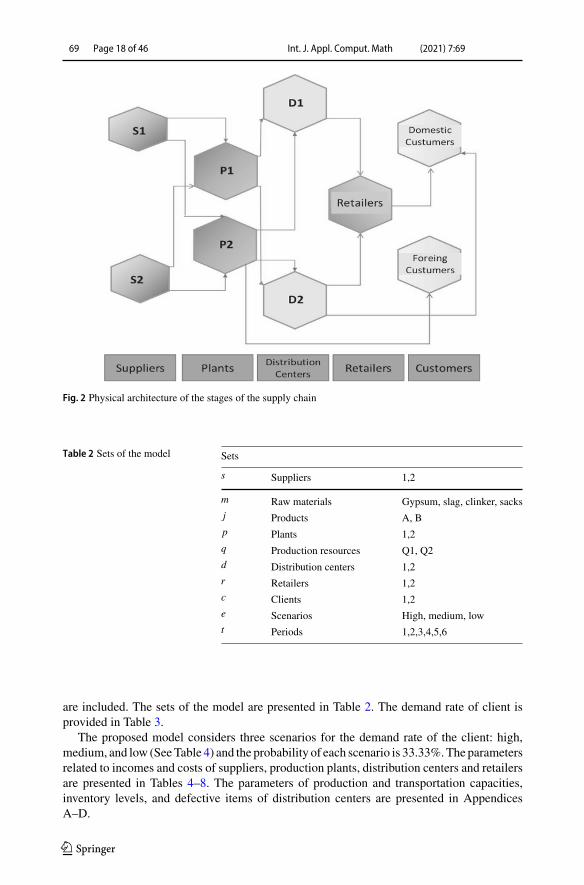
Table 2 Sets of the model Sets
s Suppliers 1,2
m Raw materials Gypsum, slag, clinker, sacksj Products A, Bp Plants 1,2q Production resources Q1, Q2d Distribution centers 1,2r Retailers 1,2c Clients 1,2e Scenarios High, medium, lowt Periods 1,2,3,4,5,6
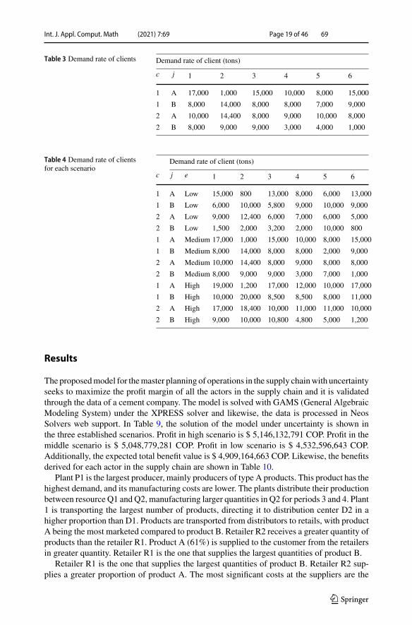
are included. The sets of the model are presented in Table 2. The demand rate of client isprovided in Table 3.
The proposed model considers three scenarios for the demand rate of the client: high,medium, and low (SeeTable 4) and the probability of each scenario is 33.33%.The parametersrelated to incomes and costs of suppliers, production plants, distribution centers and retailersare presented in Tables 4–8. The parameters of production and transportation capacities,inventory levels, and defective items of distribution centers are presented in AppendicesA–D.
123
Int. J. Appl. Comput. Math (2021) 7:69 Page 19 of 46 69
Table 3 Demand rate of clients Demand rate of client (tons)
c j 1 2 3 4 5 6
1 A 17,000 1,000 15,000 10,000 8,000 15,000
1 B 8,000 14,000 8,000 8,000 7,000 9,000
2 A 10,000 14,400 8,000 9,000 10,000 8,000
2 B 8,000 9,000 9,000 3,000 4,000 1,000
Table 4 Demand rate of clientsfor each scenario
Demand rate of client (tons)
c j e 1 2 3 4 5 6
1 A Low 15,000 800 13,000 8,000 6,000 13,000
1 B Low 6,000 10,000 5,800 9,000 10,000 9,000
2 A Low 9,000 12,400 6,000 7,000 6,000 5,000
2 B Low 1,500 2,000 3,200 2,000 10,000 800
1 A Medium 17,000 1,000 15,000 10,000 8,000 15,000
1 B Medium 8,000 14,000 8,000 8,000 2,000 9,000
2 A Medium 10,000 14,400 8,000 9,000 8,000 8,000
2 B Medium 8,000 9,000 9,000 3,000 7,000 1,000
1 A High 19,000 1,200 17,000 12,000 10,000 17,000
1 B High 10,000 20,000 8,500 8,500 8,000 11,000
2 A High 17,000 18,400 10,000 11,000 11,000 10,000
2 B High 9,000 10,000 10,800 4,800 5,000 1,200
Results
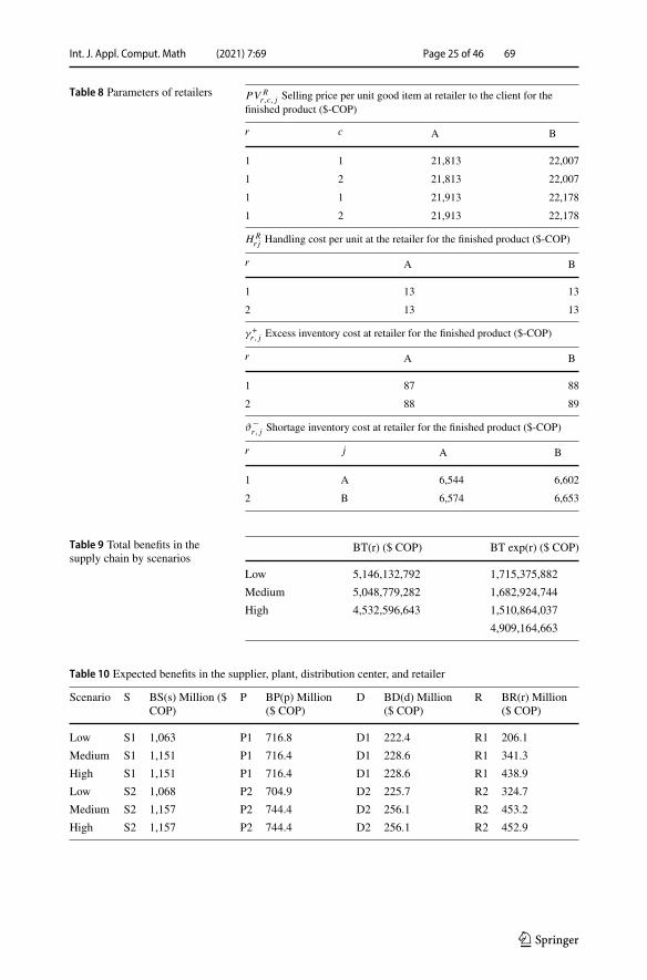
The proposedmodel for themaster planning of operations in the supply chainwith uncertaintyseeks to maximize the profit margin of all the actors in the supply chain and it is validatedthrough the data of a cement company. The model is solved with GAMS (General AlgebraicModeling System) under the XPRESS solver and likewise, the data is processed in NeosSolvers web support. In Table 9, the solution of the model under uncertainty is shown inthe three established scenarios. Profit in high scenario is $ 5,146,132,791 COP. Profit in themiddle scenario is $ 5,048,779,281 COP. Profit in low scenario is $ 4,532,596,643 COP.Additionally, the expected total benefit value is $ 4,909,164,663 COP. Likewise, the benefitsderived for each actor in the supply chain are shown in Table 10.
Plant P1 is the largest producer, mainly producers of type A products. This product has thehighest demand, and its manufacturing costs are lower. The plants distribute their productionbetween resource Q1 and Q2, manufacturing larger quantities in Q2 for periods 3 and 4. Plant1 is transporting the largest number of products, directing it to distribution center D2 in ahigher proportion than D1. Products are transported from distributors to retails, with productA being the most marketed compared to product B. Retailer R2 receives a greater quantity ofproducts than the retailer R1. Product A (61%) is supplied to the customer from the retailersin greater quantity. Retailer R1 is the one that supplies the largest quantities of product B.
Retailer R1 is the one that supplies the largest quantities of product B. Retailer R2 sup-plies a greater proportion of product A. The most significant costs at the suppliers are the
123
69 Page 20 of 46 Int. J. Appl. Comput. Math (2021) 7:69
Table 5 Parameters of suppliers
PV Ss,p,m Selling price of raw material ($- COP)
s p Gypsum Slag Clinker Sacks
1 1 20,825 20,298 59,358 2,958,501
1 2 20,825 20,298 59,358 2,958,501
2 1 20,630 20,546 59,849 2,988,086
2 2 20,630 20,546 59,894 2,988,086
PV DSs,p,m Selling price per unit defective item ($-COP)
s p Gypsum Slag Clinker
1 1 13,101 11,979 44,712
2 1 12,958 12,158 44,809
CPSs,m,t Production cost per unit of raw material ($-COP)
s m 1 2 3 4 5 6
1 Gypsum 1,101 1,101 1,101 1,101 1,101 1,101
1 Slag 1,979 1,979 1,979 1,979 1,979 1,979
1 Clinker 4,712 4,712 4,712 4,712 4,712 4,712
1 Sacks 218,876 218,876 218,876 218,876 218,876 218,876
2 Gypsum 1,101 1,101 1,101 1,101 1,101 1,101
2 Slag 1,979 1,979 1,979 1,979 1,979 1,979
2 Clinker 4,712 4,712 4,712 4,712 4,712 4,712
2 Sacks 218,876 218,876 218,876 218,876 218,876 218,876
CTSs,p,m Transportation cost per unit from the supplier to production plant ($- COP)
s p Gypsum Slag Clinker Sacks
1 1 3,374 3,099 1,200 69,344
1 2 3,585 3,148 1,150 70,037
2 1 3,189 3,281 1,230 69,691
2 2 3,368 3,292 1,180 68,994
HSs,m Handling cost per unit at supplier for the raw material ($-COP)
s Gypsum Slag Clinker Sacks
1 641 500 483 6,693
2 565 630 579 6,760
π+s,m Inventory excess cost at supplier for the raw material ($-COP)
s Gypsum Slag Clinker Sacks
1 367 276 430 8,284
123
Int. J. Appl. Comput. Math (2021) 7:69 Page 21 of 46 69
Table 5 continued
π+s,m Inventory excess cost at supplier for the raw material ($-COP)
s Gypsum Slag Clinker Sacks
2 251 269 383 8,367
π−s,m Inventory shortage cost at supplier for the raw material ($-COP)
s Gypsum Slag Clinker Sacks
1 5,348 4,889 16,607 887,550
2 5,289 4,964 16,408 887,550
CDSs,m Disposal cost per unit defective item at supplier for raw material ($-COP)
s Gypsum Slag Clinker Sacks
1 367 276 430 284
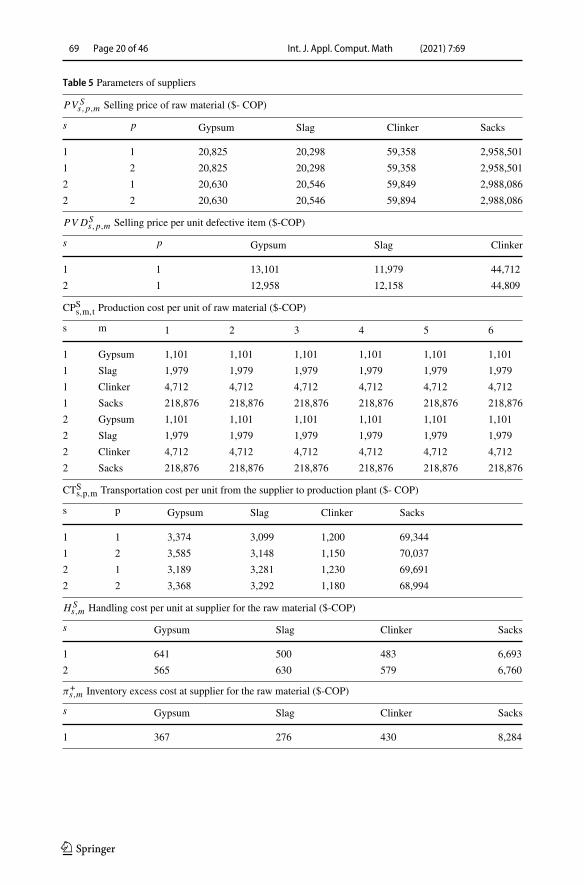
2 251 269 383 367
manufacturing costs of the raw material. The costs associated with detecting defective rawmaterial at the supplier are higher in S2 since a greater quantity is handled. The costs ofpurchasing raw materials represent an important part of the costs. Manufacturing costs arealso important within the total costs since the cement manufacturing process involves highenergy consumption.
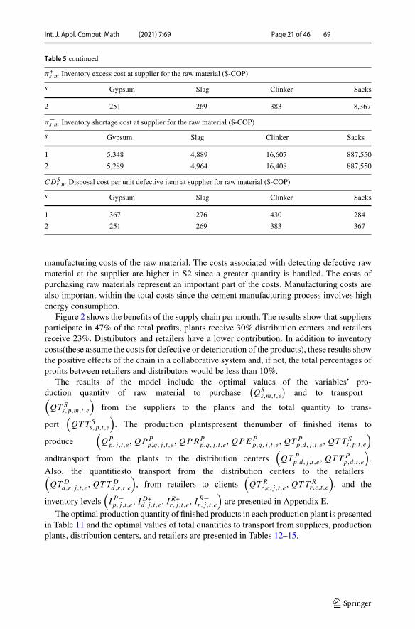
Figure 2 shows the benefits of the supply chain per month. The results show that suppliersparticipate in 47% of the total profits, plants receive 30%,distribution centers and retailersreceive 23%. Distributors and retailers have a lower contribution. In addition to inventorycosts(these assume the costs for defective or deterioration of the products), these results showthe positive effects of the chain in a collaborative system and, if not, the total percentages ofprofits between retailers and distributors would be less than 10%.
The results of the model include the optimal values of the variables’ pro-duction quantity of raw material to purchase
(QS
s,m,t,e
)and to transport(
QT Ss,p,m,t,e
)from the suppliers to the plants and the total quantity to trans-
port(QTT S
s,p,t,e
). The production plantspresent thenumber of finished items to
produce(QP
p, j,t,e, QPPp,q, j,t,e, QPRP
p,q, j,t,e, QPEPp,q, j,t,e, QT P
p,d, j,t,e, QTT Ss,p,t,e
)
andtransport from the plants to the distribution centers(QT P
p,d, j,t,e, QTT Pp,d,t,e
).
Also, the quantitiesto transport from the distribution centers to the retailers(QT D
d,r , j,t,e, QTT Dd,r ,t,e
), from retailers to clients
(QT R
r ,c, j,t,e, QTT Rr ,c,t,e
), and the
inventory levels(I P−p, j,t,e, I
D+d, j,t,e, I
R+r , j,t,e, I
R−r , j,t,e
)are presented in Appendix E.
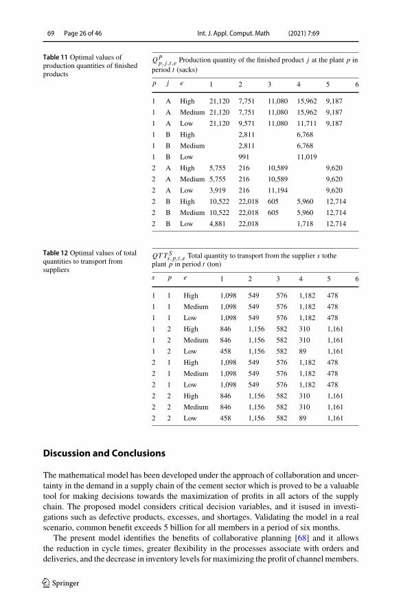
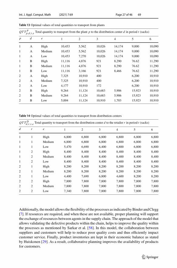
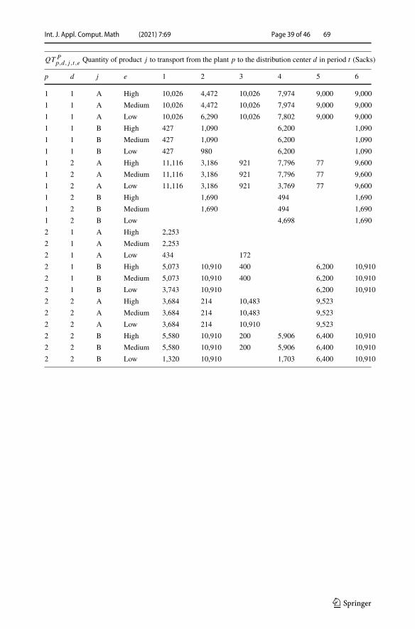
The optimal production quantity of finished products in each production plant is presentedin Table 11 and the optimal values of total quantities to transport from suppliers, productionplants, distribution centers, and retailers are presented in Tables 12–15.
123
69 Page 22 of 46 Int. J. Appl. Comput. Math (2021) 7:69
Table 6 Parameters of production plants
PV Pp,d, j Selling price per unit good item at production plant ($-COP)
p d A B
1 1 12,907 13,022
1 2 12,907 13,022
2 1 12,505 13,210
2 2 12,505 13,210
PV DPp,d, j Selling price per unit defective item at production plant ($-COP)
p d A B
1 1 9,680 9,766
1 2 9,680 9,766
2 1 9,449 9,684
2 2 9,449 9,684
CPRPp,q, j,t Production cost per unit at the production plant for the finished product working
in regular time ($-COP)
p q j 1 2 3 4 5 6
1 Q1 A 4,374 4,577 4,741 4,316 4,697 4,588
1 Q1 B 4,340 4,250 4,843 4,078 4,514 4,472
1 Q2 A 4,505 4,848 4,104 4,282 4,591 4,087
1 Q2 B 4,751 4,508 4,446 4,972 4,824 4,269
2 Q1 A 4,737 4,201 4,693 4,351 4,031 4,525
2 Q1 B 4,710 4,224 4,940 4,739 4,383 4,660
2 Q2 A 4,241 4,320 4,068 4,738 4,033 4,724
2 Q2 B 4,972 4,449 4,779 4,706 4,402 4,409
CPEPp,q, j,t Production cost per unit at the production plant for the finished product working
in extra time ($-COP)
p q j 1 2 3 4 5 6
1 Q1 A 14,374 14,577 4,741 4,316 4,697 4,588
1 Q1 B 14,340 14,250 4,843 4,078 4,514 4,472
1 Q2 A 14,505 14,848 4,104 4,282 4,591 4,087
1 Q2 B 14,751 14,508 4,446 4,972 4,824 4,269
2 Q1 A 14,737 14,201 4,693 4,351 4,031 4,525
2 Q1 B 14,710 4,224 4,940 4,739 4,383 4,660
2 Q2 A 14,241 4,320 4,068 4,738 4,033 4,724
2 Q2 B 14,972 4,449 4,779 4,706 4,402 4,409
CSubPp, j Purchasing cost per unit subcontracted by the production plant ($-COP)
p A B
1 15,000 15,000
2 15,000 15,000
123
Int. J. Appl. Comput. Math (2021) 7:69 Page 23 of 46 69
Table 6 continued
HPp, j Handling cost per unit at production plant ($-COP)
p A B
1 397 397
2 338 338
CT Pp,d, j Transportation cost per unit for the finished product from production plant to
distribution center ($-COP)
p d A B
1 1 517 517
1 2 562 562
2 1 595 595
2 2 598 598
ϕ+p, j Inventory excess cost at production plant for the finished product ($-COP)
p A B
1 444 444
2 482 482
CDPp, j Disposal cost per unit defective item at production plan for the finished product
($-COP)
p A B
1 244 244
2 215 215
ϕ−p, j Inventory shortage cost at production plant for the finished product ($-COP)
p A B
1 3,872 3,907
2 3,890 3,937
Managerial Implication
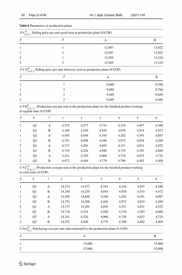
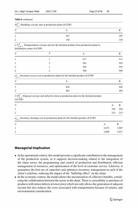
• In the operational context, thismodel presents a significant contribution to themanagementof the production system, as it supports decision-making related to the integration ofthe chain actors, the programming and control of production and distribution, efficientmanagement of resources, and optimization of the level of customer service. Likewise, itguarantees the best use of capacities and optimizes inventory management in each of thechain’s echelons, reducing the impact of the "bullwhip effect" on the chain.
• In the economic context, the model allows the maximization of collective benefits, consid-ering the collaboration between the actors in the chain. There is a possibility to purchase ofproducts withminor defects at lower price which not only allows the generation of adjacentincome but also reduces the costs associated with transportation because of returns, andenvironmental consideration.
123
69 Page 24 of 46 Int. J. Appl. Comput. Math (2021) 7:69
Table 7 Parameters of distribution centers
PV Dd,r , j Selling price per unit good item at distribution center to the retailer for the finished
product ($-COP)
d r A B
1 1 17,216 17,365
1 2 17,216 17,365
2 1 17,296 17,500
2 2 17,296 17,500
CT Dd,r , j Fixed transportation cost per unit from distribution center d to the retailer r for the finished product
($-COP)
d r A B
1 1 314 314
1 2 338 338
2 1 315 315
2 2 342 342
HDd, j Handling cost per unit at the distribution center for the finished product ($-COP)
d A B
1 22 22
2 23 23
γ +d, j Excess inventory cost at distribution center for the finished product ($-COP)
d A B
1 69 69
2 69 69
γ −d, j Shortage inventory cost at distribution center for the finished product ($-COP)
d A B
1 5,165 5,209
2 5,189 5,250
CDDd, j Disposal cost per unit defective item at distribution center for the finished product ($-COP)
d A B
1 840 840
2 820 820
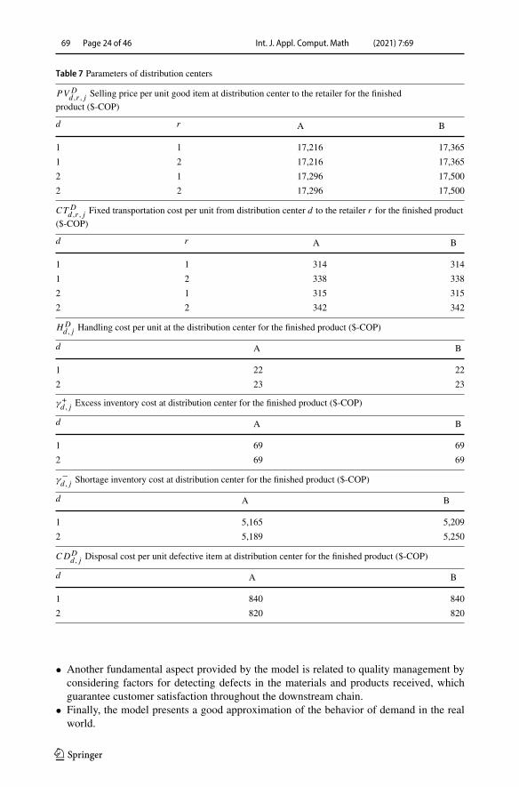
• Another fundamental aspect provided by the model is related to quality management byconsidering factors for detecting defects in the materials and products received, whichguarantee customer satisfaction throughout the downstream chain.
• Finally, the model presents a good approximation of the behavior of demand in the realworld.
123
Int. J. Appl. Comput. Math (2021) 7:69 Page 25 of 46 69
Table 8 Parameters of retailers PV Rr,c, j Selling price per unit good item at retailer to the client for the
finished product ($-COP)
r c A B
1 1 21,813 22,007
1 2 21,813 22,007
1 1 21,913 22,178
1 2 21,913 22,178
HRr j Handling cost per unit at the retailer for the finished product ($-COP)
r A B
1 13 13
2 13 13
γ +r, j Excess inventory cost at retailer for the finished product ($-COP)
r A B
1 87 88
2 88 89
ϑ−r, j Shortage inventory cost at retailer for the finished product ($-COP)
r j A B
1 A 6,544 6,602
2 B 6,574 6,653
Table 9 Total benefits in thesupply chain by scenarios
BT(r) ($ COP) BT exp(r) ($ COP)
Low 5,146,132,792 1,715,375,882
Medium 5,048,779,282 1,682,924,744
High 4,532,596,643 1,510,864,037
4,909,164,663
Table 10 Expected benefits in the supplier, plant, distribution center, and retailer
Scenario S BS(s) Million ($COP)
P BP(p) Million($ COP)
D BD(d) Million($ COP)
R BR(r) Million($ COP)
Low S1 1,063 P1 716.8 D1 222.4 R1 206.1
Medium S1 1,151 P1 716.4 D1 228.6 R1 341.3
High S1 1,151 P1 716.4 D1 228.6 R1 438.9
Low S2 1,068 P2 704.9 D2 225.7 R2 324.7
Medium S2 1,157 P2 744.4 D2 256.1 R2 453.2
High S2 1,157 P2 744.4 D2 256.1 R2 452.9
123
69 Page 26 of 46 Int. J. Appl. Comput. Math (2021) 7:69
Table 11 Optimal values ofproduction quantities of finishedproducts
QPp, j ,t,e Production quantity of the finished product j at the plant p in
period t (sacks)
p j e 1 2 3 4 5 6
1 A High 21,120 7,751 11,080 15,962 9,187
1 A Medium 21,120 7,751 11,080 15,962 9,187
1 A Low 21,120 9,571 11,080 11,711 9,187
1 B High 2,811 6,768
1 B Medium 2,811 6,768
1 B Low 991 11,019
2 A High 5,755 216 10,589 9,620
2 A Medium 5,755 216 10,589 9,620
2 A Low 3,919 216 11,194 9,620
2 B High 10,522 22,018 605 5,960 12,714
2 B Medium 10,522 22,018 605 5,960 12,714
2 B Low 4,881 22,018 1,718 12,714
Table 12 Optimal values of totalquantities to transport fromsuppliers
QTT Ss,p,t,e Total quantity to transport from the supplier s tothe
plant p in period t (ton)
s p e 1 2 3 4 5 6
1 1 High 1,098 549 576 1,182 478
1 1 Medium 1,098 549 576 1,182 478
1 1 Low 1,098 549 576 1,182 478
1 2 High 846 1,156 582 310 1,161
1 2 Medium 846 1,156 582 310 1,161
1 2 Low 458 1,156 582 89 1,161
2 1 High 1,098 549 576 1,182 478
2 1 Medium 1,098 549 576 1,182 478
2 1 Low 1,098 549 576 1,182 478
2 2 High 846 1,156 582 310 1,161
2 2 Medium 846 1,156 582 310 1,161
2 2 Low 458 1,156 582 89 1,161
Discussion and Conclusions
The mathematical model has been developed under the approach of collaboration and uncer-tainty in the demand in a supply chain of the cement sector which is proved to be a valuabletool for making decisions towards the maximization of profits in all actors of the supplychain. The proposed model considers critical decision variables, and it isused in investi-gations such as defective products, excesses, and shortages. Validating the model in a realscenario, common benefit exceeds 5 billion for all members in a period of six months.
The present model identifies the benefits of collaborative planning [68] and it allowsthe reduction in cycle times, greater flexibility in the processes associate with orders anddeliveries, and the decrease in inventory levels for maximizing the profit of channel members.
123
Int. J. Appl. Comput. Math (2021) 7:69 Page 27 of 46 69
Table 13 Optimal values of total quantities to transport from plants
QTT Pp,d,t,e Total quantity to transport from the plant p to the distribution center d in period t (sacks)
p d e 1 2 3 4 5 6
1 A High 10,453 5,562 10,026 14,174 9,000 10,090
1 A Medium 10,453 5,562 10,026 14,174 9,000 10,090
1 A Low 10,453 7,270 10,026 14,174 9,000 10,090
1 B High 11,116 4,876 921 8,290 76.62 11,290
1 B Medium 11,116 4,876 921 8,290 76.62 11,290
1 B Low 11,116 3,166 921 8,466 76.62 11,290
2 A High 7,325 10,910 400 6,200 10,910
2 A Medium 7,325 10,910 400 6,200 10,910
2 A Low 4,177 10,910 172 6,200 10,910
2 B High 9,264 11,124 10,683 5,906 15,923 10,910
2 B Medium 9,264 11,124 10,683 5,906 15,923 10,910
2 B Low 5,004 11,124 10,910 1,703 15,923 10,910
Table 14 Optimal values of total quantities to transport from distribution centers
QTT Dd,r ,t,e Total quantity to transport from the distribution center d to the retailer r in period t (sacks)
d r e 1 2 3 4 5 6
1 1 High 6,800 6,800 6,800 6,800 6,800 6,800
1 1 Medium 6,800 6,800 6,800 6,800 6,800 6,800
1 1 Low 5,470 6,690 6,400 6,800 6,800 6,800
1 2 High 8,400 8,400 8,400 8,400 8,400 8,400
1 2 Medium 8,400 8,400 8,400 8,400 8,400 8,400
1 2 Low 8,400 8,400 8,400 8,400 8,400 8,400
2 1 High 8,200 8,200 8,200 8,200 8,200 8,200
2 1 Medium 8,200 8,200 8,200 8,200 8,200 8,200
2 1 Low 4,400 7,690 6,800 4,600 8,200 8,200
2 2 High 7,800 7,800 7,800 7,800 7,800 7,800
2 2 Medium 7,800 7,800 7,800 7,800 7,800 7,800
2 2 Low 7,340 7,800 7,800 7,800 7,800 7,800
Additionally, themodel allows theflexibility of the processes as indicatedbyBinder andClegg[7]. If resources are required, and when these are not available, proper planning will supportthe exchange of resources between agents in the supply chain. The approach of themodel thatallows validating the defective products within the chain, helps to improve the quality withinthe processes as mentioned by Sarkar et al. [58]. In this model, the collaboration betweensuppliers and customers will help to reduce poor quality costs and thus efficiently impactcustomer service. Finally, product inventories are kept in their economic balance as statedby Huiskonen [29]. As a result, collaborative planning improves the availability of productsfor customers.
123
69 Page 28 of 46 Int. J. Appl. Comput. Math (2021) 7:69
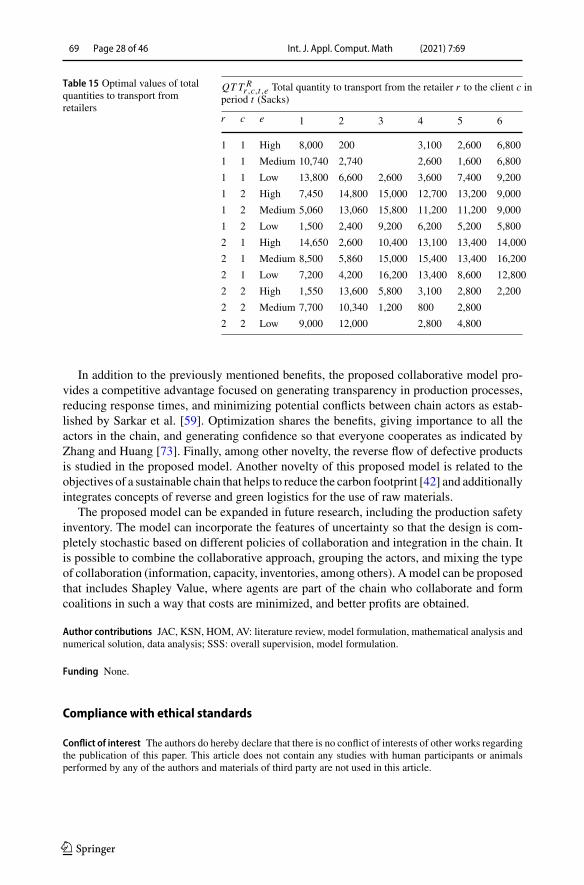
Table 15 Optimal values of totalquantities to transport fromretailers
QTT Rr ,c,t,e Total quantity to transport from the retailer r to the client c in
period t (Sacks)
r c e 1 2 3 4 5 6
1 1 High 8,000 200 3,100 2,600 6,800
1 1 Medium 10,740 2,740 2,600 1,600 6,800
1 1 Low 13,800 6,600 2,600 3,600 7,400 9,200
1 2 High 7,450 14,800 15,000 12,700 13,200 9,000
1 2 Medium 5,060 13,060 15,800 11,200 11,200 9,000
1 2 Low 1,500 2,400 9,200 6,200 5,200 5,800
2 1 High 14,650 2,600 10,400 13,100 13,400 14,000
2 1 Medium 8,500 5,860 15,000 15,400 13,400 16,200
2 1 Low 7,200 4,200 16,200 13,400 8,600 12,800
2 2 High 1,550 13,600 5,800 3,100 2,800 2,200
2 2 Medium 7,700 10,340 1,200 800 2,800
2 2 Low 9,000 12,000 2,800 4,800
In addition to the previously mentioned benefits, the proposed collaborative model pro-vides a competitive advantage focused on generating transparency in production processes,reducing response times, and minimizing potential conflicts between chain actors as estab-lished by Sarkar et al. [59]. Optimization shares the benefits, giving importance to all theactors in the chain, and generating confidence so that everyone cooperates as indicated byZhang and Huang [73]. Finally, among other novelty, the reverse flow of defective productsis studied in the proposed model. Another novelty of this proposed model is related to theobjectives of a sustainable chain that helps to reduce the carbon footprint [42] and additionallyintegrates concepts of reverse and green logistics for the use of raw materials.
The proposed model can be expanded in future research, including the production safetyinventory. The model can incorporate the features of uncertainty so that the design is com-pletely stochastic based on different policies of collaboration and integration in the chain. Itis possible to combine the collaborative approach, grouping the actors, and mixing the typeof collaboration (information, capacity, inventories, among others). Amodel can be proposedthat includes Shapley Value, where agents are part of the chain who collaborate and formcoalitions in such a way that costs are minimized, and better profits are obtained.
Author contributions JAC, KSN, HOM, AV: literature review, model formulation, mathematical analysis andnumerical solution, data analysis; SSS: overall supervision, model formulation.
Funding None.
Compliance with ethical standards
Conflict of interest The authors do hereby declare that there is no conflict of interests of other works regardingthe publication of this paper. This article does not contain any studies with human participants or animalsperformed by any of the authors and materials of third party are not used in this article.
123
Int. J. Appl. Comput. Math (2021) 7:69 Page 29 of 46 69
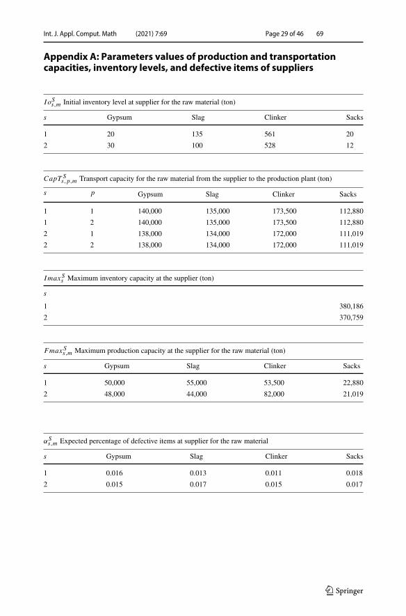
Appendix A: Parameters values of production and transportationcapacities, inventory levels, and defective items of suppliers
I oSs,m Initial inventory level at supplier for the raw material (ton)
s Gypsum Slag Clinker Sacks
1 20 135 561 20
2 30 100 528 12
CapT Ss,p,m Transport capacity for the raw material from the supplier to the production plant (ton)
s p Gypsum Slag Clinker Sacks
1 1 140,000 135,000 173,500 112,880
1 2 140,000 135,000 173,500 112,880
2 1 138,000 134,000 172,000 111,019
2 2 138,000 134,000 172,000 111,019
ImaxSs Maximum inventory capacity at the supplier (ton)
s
1 380,186
2 370,759
FmaxSs,m Maximum production capacity at the supplier for the raw material (ton)
s Gypsum Slag Clinker Sacks
1 50,000 55,000 53,500 22,880
2 48,000 44,000 82,000 21,019
αSs,m Expected percentage of defective items at supplier for the raw material
s Gypsum Slag Clinker Sacks
1 0.016 0.013 0.011 0.018
2 0.015 0.017 0.015 0.017
123
69 Page 30 of 46 Int. J. Appl. Comput. Math (2021) 7:69
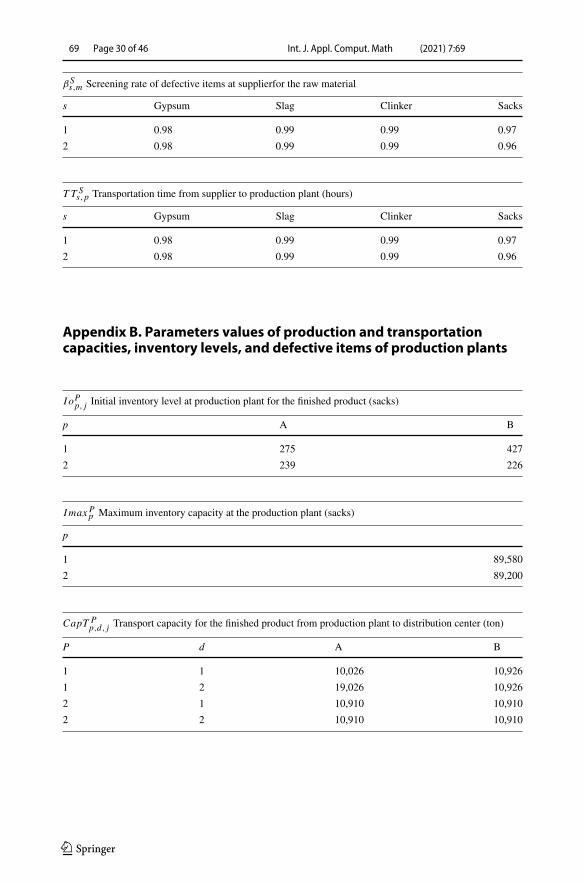
βSs,m Screening rate of defective items at supplierfor the raw material
s Gypsum Slag Clinker Sacks
1 0.98 0.99 0.99 0.97
2 0.98 0.99 0.99 0.96
T T Ss,p Transportation time from supplier to production plant (hours)
s Gypsum Slag Clinker Sacks
1 0.98 0.99 0.99 0.97
2 0.98 0.99 0.99 0.96
Appendix B. Parameters values of production and transportationcapacities, inventory levels, and defective items of production plants
I oPp, j Initial inventory level at production plant for the finished product (sacks)
p A B
1 275 427
2 239 226
Imax Pp Maximum inventory capacity at the production plant (sacks)
p
1 89,580
2 89,200
CapT Pp,d, j Transport capacity for the finished product from production plant to distribution center (ton)
P d A B
1 1 10,026 10,926
1 2 19,026 10,926
2 1 10,910 10,910
2 2 10,910 10,910
123
Int. J. Appl. Comput. Math (2021) 7:69 Page 31 of 46 69
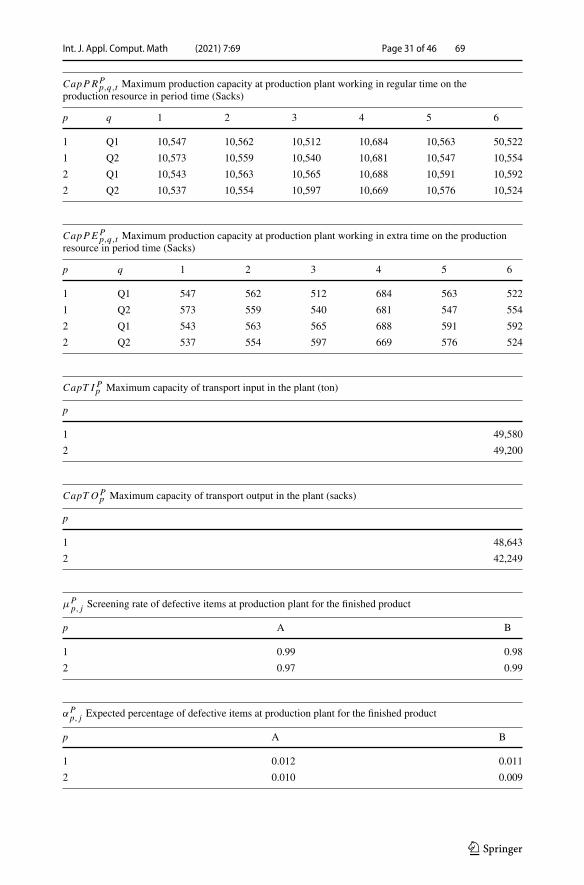
CapPRPp,q,t Maximum production capacity at production plant working in regular time on the
production resource in period time (Sacks)
p q 1 2 3 4 5 6
1 Q1 10,547 10,562 10,512 10,684 10,563 50,522
1 Q2 10,573 10,559 10,540 10,681 10,547 10,554
2 Q1 10,543 10,563 10,565 10,688 10,591 10,592
2 Q2 10,537 10,554 10,597 10,669 10,576 10,524
CapPEPp,q,t Maximum production capacity at production plant working in extra time on the production
resource in period time (Sacks)
p q 1 2 3 4 5 6
1 Q1 547 562 512 684 563 522
1 Q2 573 559 540 681 547 554
2 Q1 543 563 565 688 591 592
2 Q2 537 554 597 669 576 524
CapT I Pp Maximum capacity of transport input in the plant (ton)
p
1 49,580
2 49,200
CapT OPp Maximum capacity of transport output in the plant (sacks)
p
1 48,643
2 42,249
μPp, j Screening rate of defective items at production plant for the finished product
p A B
1 0.99 0.98
2 0.97 0.99
αPp, j Expected percentage of defective items at production plant for the finished product
p A B
1 0.012 0.011
2 0.010 0.009
123
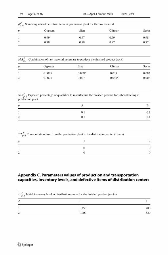
69 Page 32 of 46 Int. J. Appl. Comput. Math (2021) 7:69
βPp.m Screening rate of defective items at production plant for the raw material
p Gypsum Slag Clinker Sacks
1 0.99 0.97 0.99 0.98
2 0.98 0.98 0.97 0.97
MAPm, j Combination of raw material necessary to produce the finished product (sack)
p Gypsum Slag Clinker Sacks
1 0.0025 0.0095 0.038 0.002
2 0.0025 0.007 0.0405 0.002
SubPp, j Expected percentage of quantities to manufacture the finished product for subcontracting atproduction plant
p A B
1 0.1 0.1
2 0.1 0.1
T T Pp,d Transportation time from the production plant to the distribution center (Hours)
p 1 2
1 0 0
2 0 0
Appendix C. Parameters values of production and transportationcapacities, inventory levels, and defective items of distribution centers
I oDd, j Initial inventory level at distribution center for the finished product (sacks)
d 1 2
1 1,250 700
2 1,000 820
123
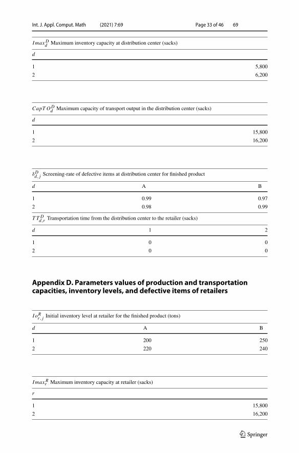
Int. J. Appl. Comput. Math (2021) 7:69 Page 33 of 46 69
ImaxDd Maximum inventory capacity at distribution center (sacks)
d
1 5,800
2 6,200
CapT ODd Maximum capacity of transport output in the distribution center (sacks)
d
1 15,800
2 16,200
δDd, j Screening-rate of defective items at distribution center for finished product
d A B
1 0.99 0.97
2 0.98 0.99
T T Dd,r Transportation time from the distribution center to the retailer (sacks)
d 1 2
1 0 0
2 0 0
Appendix D. Parameters values of production and transportationcapacities, inventory levels, and defective items of retailers
I oRr , j Initial inventory level at retailer for the finished product (tons)
d A B
1 200 250
2 220 240
Imax Rr Maximum inventory capacity at retailer (sacks)
r
1 15,800
2 16,200
123
69 Page 34 of 46 Int. J. Appl. Comput. Math (2021) 7:69
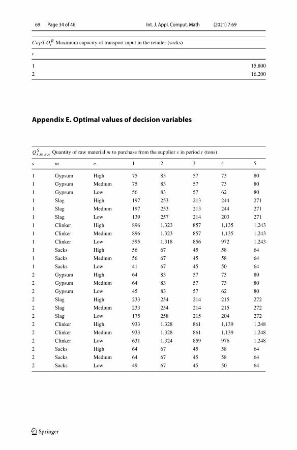
CapT ORr Maximum capacity of transport input in the retailer (sacks)
r
1 15,800
2 16,200
Appendix E. Optimal values of decision variables
QSs,m,t,e Quantity of raw material m to purchase from the supplier s in period t (tons)
s m e 1 2 3 4 5
1 Gypsum High 75 83 57 73 80
1 Gypsum Medium 75 83 57 73 80
1 Gypsum Low 56 83 57 62 80
1 Slag High 197 253 213 244 271
1 Slag Medium 197 253 213 244 271
1 Slag Low 139 257 214 203 271
1 Clinker High 896 1,323 857 1,135 1,243
1 Clinker Medium 896 1,323 857 1,135 1,243
1 Clinker Low 595 1,318 856 972 1,243
1 Sacks High 56 67 45 58 64
1 Sacks Medium 56 67 45 58 64
1 Sacks Low 41 67 45 50 64
2 Gypsum High 64 83 57 73 80
2 Gypsum Medium 64 83 57 73 80
2 Gypsum Low 45 83 57 62 80
2 Slag High 233 254 214 215 272
2 Slag Medium 233 254 214 215 272
2 Slag Low 175 258 215 204 272
2 Clinker High 933 1,328 861 1,139 1,248
2 Clinker Medium 933 1,328 861 1,139 1,248
2 Clinker Low 631 1,324 859 976 1,248
2 Sacks High 64 67 45 58 64
2 Sacks Medium 64 67 45 58 64
2 Sacks Low 49 67 45 50 64
123
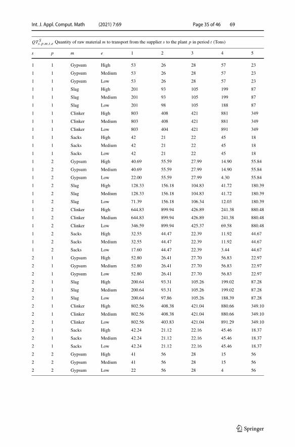
Int. J. Appl. Comput. Math (2021) 7:69 Page 35 of 46 69
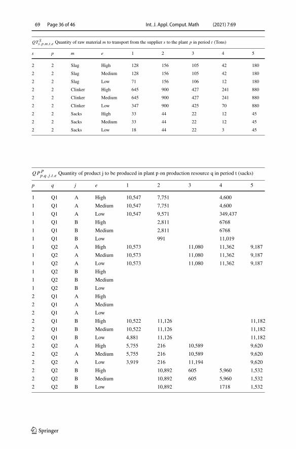
QT Ss.p.m.t .e Quantity of raw material m to transport from the supplier s to the plant p in period t (Tons)
s p m e 1 2 3 4 5
1 1 Gypsum High 53 26 28 57 23
1 1 Gypsum Medium 53 26 28 57 23
1 1 Gypsum Low 53 26 28 57 23
1 1 Slag High 201 93 105 199 87
1 1 Slag Medium 201 93 105 199 87
1 1 Slag Low 201 98 105 188 87
1 1 Clinker High 803 408 421 881 349
1 1 Clinker Medium 803 408 421 881 349
1 1 Clinker Low 803 404 421 891 349
1 1 Sacks High 42 21 22 45 18
1 1 Sacks Medium 42 21 22 45 18
1 1 Sacks Low 42 21 22 45 18
1 2 Gypsum High 40.69 55.59 27.99 14.90 55.84
1 2 Gypsum Medium 40.69 55.59 27.99 14.90 55.84
1 2 Gypsum Low 22.00 55.59 27.99 4.30 55.84
1 2 Slag High 128.33 156.18 104.83 41.72 180.39
1 2 Slag Medium 128.33 156.18 104.83 41.72 180.39
1 2 Slag Low 71.39 156.18 106.34 12.03 180.39
1 2 Clinker High 644.83 899.94 426.89 241.38 880.48
1 2 Clinker Medium 644.83 899.94 426.89 241.38 880.48
1 2 Clinker Low 346.59 899.94 425.37 69.58 880.48
1 2 Sacks High 32.55 44.47 22.39 11.92 44.67
1 2 Sacks Medium 32.55 44.47 22.39 11.92 44.67
1 2 Sacks Low 17.60 44.47 22.39 3.44 44.67
2 1 Gypsum High 52.80 26.41 27.70 56.83 22.97
2 1 Gypsum Medium 52.80 26.41 27.70 56.83 22.97
2 1 Gypsum Low 52.80 26.41 27.70 56.83 22.97
2 1 Slag High 200.64 93.31 105.26 199.02 87.28
2 1 Slag Medium 200.64 93.31 105.26 199.02 87.28
2 1 Slag Low 200.64 97.86 105.26 188.39 87.28
2 1 Clinker High 802.56 408.38 421.04 880.66 349.10
2 1 Clinker Medium 802.56 408.38 421.04 880.66 349.10
2 1 Clinker Low 802.56 403.83 421.04 891.29 349.10
2 1 Sacks High 42.24 21.12 22.16 45.46 18.37
2 1 Sacks Medium 42.24 21.12 22.16 45.46 18.37
2 1 Sacks Low 42.24 21.12 22.16 45.46 18.37
2 2 Gypsum High 41 56 28 15 56
2 2 Gypsum Medium 41 56 28 15 56
2 2 Gypsum Low 22 56 28 4 56
123
69 Page 36 of 46 Int. J. Appl. Comput. Math (2021) 7:69
QT Ss.p.m.t .e Quantity of raw material m to transport from the supplier s to the plant p in period t (Tons)
s p m e 1 2 3 4 5
2 2 Slag High 128 156 105 42 180
2 2 Slag Medium 128 156 105 42 180
2 2 Slag Low 71 156 106 12 180
2 2 Clinker High 645 900 427 241 880
2 2 Clinker Medium 645 900 427 241 880
2 2 Clinker Low 347 900 425 70 880
2 2 Sacks High 33 44 22 12 45
2 2 Sacks Medium 33 44 22 12 45
2 2 Sacks Low 18 44 22 3 45
QPPp.q. j .t .e Quantity of product j to be produced in plant p on production resource q in period t (sacks)
p q j e 1 2 3 4 5
1 Q1 A High 10,547 7,751 4,600
1 Q1 A Medium 10,547 7,751 4,600
1 Q1 A Low 10,547 9,571 349,437
1 Q1 B High 2,811 6768
1 Q1 B Medium 2,811 6768
1 Q1 B Low 991 11,019
1 Q2 A High 10,573 11,080 11,362 9,187
1 Q2 A Medium 10,573 11,080 11,362 9,187
1 Q2 A Low 10,573 11,080 11,362 9,187
1 Q2 B High
1 Q2 B Medium
1 Q2 B Low
2 Q1 A High
2 Q1 A Medium
2 Q1 A Low
2 Q1 B High 10,522 11,126 11,182
2 Q1 B Medium 10,522 11,126 11,182
2 Q1 B Low 4,881 11,126 11,182
2 Q2 A High 5,755 216 10,589 9,620
2 Q2 A Medium 5,755 216 10,589 9,620
2 Q2 A Low 3,919 216 11,194 9,620
2 Q2 B High 10,892 605 5,960 1,532
2 Q2 B Medium 10,892 605 5,960 1,532
2 Q2 B Low 10,892 1718 1,532
123
Int. J. Appl. Comput. Math (2021) 7:69 Page 37 of 46 69
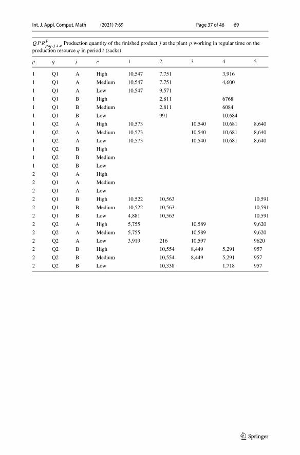
QPRPp.q. j .t .e Production quantity of the finished product j at the plant p working in regular time on the
production resource q in period t (sacks)
p q j e 1 2 3 4 5
1 Q1 A High 10,547 7.751 3,916
1 Q1 A Medium 10,547 7.751 4,600
1 Q1 A Low 10,547 9,571
1 Q1 B High 2,811 6768
1 Q1 B Medium 2,811 6084
1 Q1 B Low 991 10,684
1 Q2 A High 10,573 10,540 10,681 8,640
1 Q2 A Medium 10,573 10,540 10,681 8,640
1 Q2 A Low 10,573 10,540 10,681 8,640
1 Q2 B High
1 Q2 B Medium
1 Q2 B Low
2 Q1 A High
2 Q1 A Medium
2 Q1 A Low
2 Q1 B High 10,522 10,563 10,591
2 Q1 B Medium 10,522 10,563 10,591
2 Q1 B Low 4,881 10,563 10,591
2 Q2 A High 5,755 10,589 9,620
2 Q2 A Medium 5,755 10,589 9,620
2 Q2 A Low 3,919 216 10,597 9620
2 Q2 B High 10,554 8,449 5,291 957
2 Q2 B Medium 10,554 8,449 5,291 957
2 Q2 B Low 10,338 1,718 957
123
69 Page 38 of 46 Int. J. Appl. Comput. Math (2021) 7:69
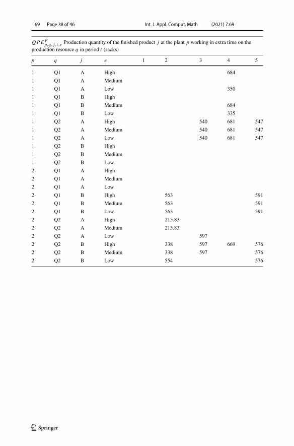
QPEPp,q, j,t,e Production quantity of the finished product j at the plant p working in extra time on the
production resource q in period t (sacks)
p q j e 1 2 3 4 5
1 Q1 A High 684
1 Q1 A Medium
1 Q1 A Low 350
1 Q1 B High
1 Q1 B Medium 684
1 Q1 B Low 335
1 Q2 A High 540 681 547
1 Q2 A Medium 540 681 547
1 Q2 A Low 540 681 547
1 Q2 B High
1 Q2 B Medium
1 Q2 B Low
2 Q1 A High
2 Q1 A Medium
2 Q1 A Low
2 Q1 B High 563 591
2 Q1 B Medium 563 591
2 Q1 B Low 563 591
2 Q2 A High 215.83
2 Q2 A Medium 215.83
2 Q2 A Low 597
2 Q2 B High 338 597 669 576
2 Q2 B Medium 338 597 576
2 Q2 B Low 554 576
123
Int. J. Appl. Comput. Math (2021) 7:69 Page 39 of 46 69
QT Pp,d, j,t,e Quantity of product j to transport from the plant p to the distribution center d in period t (Sacks)
p d j e 1 2 3 4 5 6
1 1 A High 10,026 4,472 10,026 7,974 9,000 9,000
1 1 A Medium 10,026 4,472 10,026 7,974 9,000 9,000
1 1 A Low 10,026 6,290 10,026 7,802 9,000 9,000
1 1 B High 427 1,090 6,200 1,090
1 1 B Medium 427 1,090 6,200 1,090
1 1 B Low 427 980 6,200 1,090
1 2 A High 11,116 3,186 921 7,796 77 9,600
1 2 A Medium 11,116 3,186 921 7,796 77 9,600
1 2 A Low 11,116 3,186 921 3,769 77 9,600
1 2 B High 1,690 494 1,690
1 2 B Medium 1,690 494 1,690
1 2 B Low 4,698 1,690
2 1 A High 2,253
2 1 A Medium 2,253
2 1 A Low 434 172
2 1 B High 5,073 10,910 400 6,200 10,910
2 1 B Medium 5,073 10,910 400 6,200 10,910
2 1 B Low 3,743 10,910 6,200 10,910
2 2 A High 3,684 214 10,483 9,523
2 2 A Medium 3,684 214 10,483 9,523
2 2 A Low 3,684 214 10,910 9,523
2 2 B High 5,580 10,910 200 5,906 6,400 10,910
2 2 B Medium 5,580 10,910 200 5,906 6,400 10,910
2 2 B Low 1,320 10,910 1,703 6,400 10,910
123
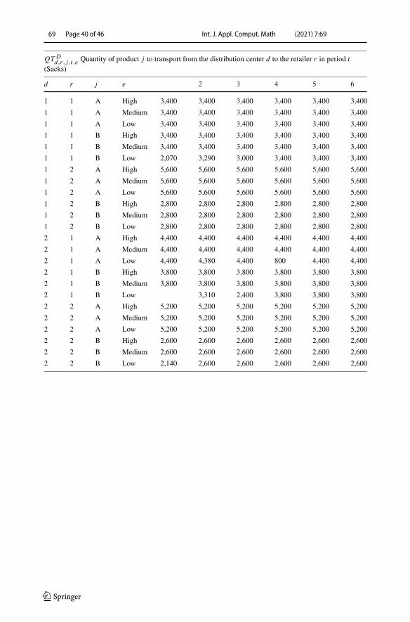
69 Page 40 of 46 Int. J. Appl. Comput. Math (2021) 7:69
QT Dd,r , j,t,e Quantity of product j to transport from the distribution center d to the retailer r in period t
(Sacks)
d r j e 2 3 4 5 6
1 1 A High 3,400 3,400 3,400 3,400 3,400 3,400
1 1 A Medium 3,400 3,400 3,400 3,400 3,400 3,400
1 1 A Low 3,400 3,400 3,400 3,400 3,400 3,400
1 1 B High 3,400 3,400 3,400 3,400 3,400 3,400
1 1 B Medium 3,400 3,400 3,400 3,400 3,400 3,400
1 1 B Low 2,070 3,290 3,000 3,400 3,400 3,400
1 2 A High 5,600 5,600 5,600 5,600 5,600 5,600
1 2 A Medium 5,600 5,600 5,600 5,600 5,600 5,600
1 2 A Low 5,600 5,600 5,600 5,600 5,600 5,600
1 2 B High 2,800 2,800 2,800 2,800 2,800 2,800
1 2 B Medium 2,800 2,800 2,800 2,800 2,800 2,800
1 2 B Low 2,800 2,800 2,800 2,800 2,800 2,800
2 1 A High 4,400 4,400 4,400 4,400 4,400 4,400
2 1 A Medium 4,400 4,400 4,400 4,400 4,400 4,400
2 1 A Low 4,400 4,380 4,400 800 4,400 4,400
2 1 B High 3,800 3,800 3,800 3,800 3,800 3,800
2 1 B Medium 3,800 3,800 3,800 3,800 3,800 3,800
2 1 B Low 3,310 2,400 3,800 3,800 3,800
2 2 A High 5,200 5,200 5,200 5,200 5,200 5,200
2 2 A Medium 5,200 5,200 5,200 5,200 5,200 5,200
2 2 A Low 5,200 5,200 5,200 5,200 5,200 5,200
2 2 B High 2,600 2,600 2,600 2,600 2,600 2,600
2 2 B Medium 2,600 2,600 2,600 2,600 2,600 2,600
2 2 B Low 2,140 2,600 2,600 2,600 2,600 2,600
123
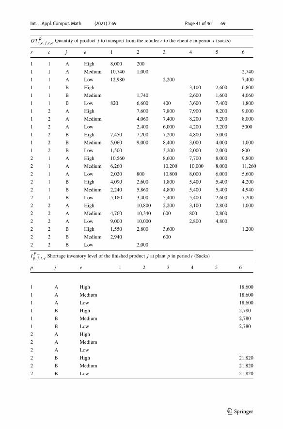
Int. J. Appl. Comput. Math (2021) 7:69 Page 41 of 46 69
QT Rr ,c, j,t,e Quantity of product j to transport from the retailer r to the client c in period t (sacks)
r c j e 1 2 3 4 5 6
1 1 A High 8,000 200
1 1 A Medium 10,740 1,000 2,740
1 1 A Low 12,980 2,200 7,400
1 1 B High 3,100 2,600 6,800
1 1 B Medium 1,740 2,600 1,600 4,060
1 1 B Low 820 6,600 400 3,600 7,400 1,800
1 2 A High 7,600 7,800 7,900 8,200 9,000
1 2 A Medium 4,060 7,400 8,200 7,200 8,000
1 2 A Low 2,400 6,000 4,200 3,200 5000
1 2 B High 7,450 7,200 7,200 4,800 5,000
1 2 B Medium 5,060 9,000 8,400 3,000 4,000 1,000
1 2 B Low 1,500 3,200 2,000 2,000 800
2 1 A High 10,560 8,600 7,700 8,000 9,800
2 1 A Medium 6,260 10,200 10,000 8,000 11,260
2 1 A Low 2,020 800 10,800 8,000 6,000 5,600
2 1 B High 4,090 2,600 1,800 5,400 5,400 4,200
2 1 B Medium 2,240 5,860 4,800 5,400 5,400 4,940
2 1 B Low 5,180 3,400 5,400 5,400 2,600 7,200
2 2 A High 10,800 2,200 3,100 2,800 1,000
2 2 A Medium 4,760 10,340 600 800 2,800
2 2 A Low 9,000 10,000 2,800 4,800
2 2 B High 1,550 2,800 3,600 1,200
2 2 B Medium 2,940 600
2 2 B Low 2,000
I P−p, j,t,e Shortage inventory level of the finished product j at plant p in period t (Sacks)
p j e 1 2 3 4 5 6
1 A High 18,600
1 A Medium 18,600
1 A Low 18,600
1 B High 2,780
1 B Medium 2,780
1 B Low 2,780
2 A High
2 A Medium
2 A Low
2 B High 21,820
2 B Medium 21,820
2 B Low 21,820
123
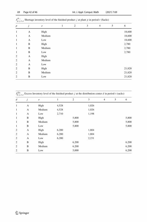
69 Page 42 of 46 Int. J. Appl. Comput. Math (2021) 7:69
I P−p, j,t,e Shortage inventory level of the finished product j at plant p in period t (Sacks)
p j e 1 2 3 4 5 6
1 A High 18,600
1 A Medium 18,600
1 A Low 18,600
1 B High 2,780
1 B Medium 2,780
1 B Low 2,780
2 A High
2 A Medium
2 A Low
2 B High 21,820
2 B Medium 21,820
2 B Low 21,820
I D+d, j,t,e Excess Inventory level of the finished product j at the distribution center d in period t (sacks)
d j e 1 2 3 4 5 6
1 A High 4,528 1,026
1 A Medium 4,528 1,026
1 A Low 2,710 1,198
1 B High 5,800 5,800
1 B Medium 5,800 5,800
1 B Low 5,800 5,800
2 A High 6,200 1,804
2 A Medium 6,200 1,804
2 A Low 6,200 2,231
2 B High 6,200 6,200
2 B Medium 6,200 6,200
2 B Low 5,000 6,200
123
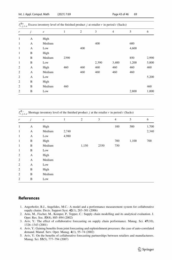
Int. J. Appl. Comput. Math (2021) 7:69 Page 43 of 46 69
I R+r , j,t,e Excess inventory level of the finished product j at retailer r in period t (Sacks)
r j e 1 2 3 4 5 6
1 A High
1 A Medium 400 600
1 A Low 400 4,600
1 B High
1 B Medium 2390 850 2,990
1 B Low 2,390 3,400 1,200 5,800
2 A High 460 460 460 460 460 460
2 A Medium 460 460 460 460
2 A Low 5,200
2 B High
2 B Medium 460 460
2 B Low 2,800 1,000
I R−r , j,t,e Shortage inventory level of the finished product j at the retailer r in period t (Sacks)
r j e 1 2 3 4 5 6
1 A High 100 500 1,700
1 A Medium 2,740 2,340
1 A Low 4,980
1 B High 700 1,100 700
1 B Medium 1,150 2350 750
1 B Low
2 A High
2 A Medium
2 A Low
2 B High
2 B Medium
2 B Low
References
1. Angerhofer, B.J., Angelides, M.C.: A model and a performance measurement system for collaborativesupply chains. Decis. Support Syst. 42(1), 283–301 (2006)
2. Arns, M., Fischer, M., Kemper, P., Tepper, C.: Supply chain modelling and its analytical evaluation. J.Oper. Res. Soc. 53(8), 885–894 (2002)
3. Aviv, Y.: The effect of collaborative forecasting on supply chain performance. Manag. Sci. 47(10),1326–1343 (2001)
4. Aviv, Y.: Gaining benefits from joint forecasting and replenishment processes: the case of auto-correlateddemand. Manuf. Serv. Oper. Manag. 4(1), 55–74 (2002)
5. Aviv, Y.: On the benefits of collaborative forecasting partnerships between retailers and manufacturers.Manag. Sci. 53(5), 777–794 (2007)
123
69 Page 44 of 46 Int. J. Appl. Comput. Math (2021) 7:69
6. Barratt, M.: Understanding the meaning of collaboration in the supply chain. Supply Chain Manag. Int.J. 9(1), 30–42 (2004)
7. Binder,M., Clegg, B.: Enterprise management: a new frontier for organisations. Int. J. Prod. Econ. 106(2),409–430 (2007)
8. Cárdenas, M., Reina, M.: La minería en Colombia: impacto socioeconómico y fiscal (2008)9. Chan, F.T., Zhang, T.: The impact of collaborative transportation management on supply chain perfor-
mance: a simulation approach. Expert Syst. Appl. 38(3), 2319–2329 (2011)10. Chedid, J.A., Vidal, G.H.: Análisis del Problema de Planificación de la Producción en Cadenas de Sum-
inistro Colaborativas: Una Revisión de la Literatura en el Enfoque de Teoría de Juegos (2012)11. Chen, C.-L., Lee,W.-C.:Multi-objective optimization ofmulti-echelon supply chain networkswith uncer-
tain product demands and prices. Comput. Chem. Eng. 28(6–7), 1131–1144 (2004)12. Chen, T.-H., Chen, J.-M.:Optimizing supply chain collaboration based on joint replenishment and channel
coordination. Transp. Res. Part E Logist. Transp. Rev. 41(4), 261–285 (2005)13. Cheung, C.F., Cheung, C., Kwok, S.: A knowledge-based customization system for supply chain integra-
tion. Expert Syst. Appl. 39(4), 3906–3924 (2012)14. Chopra, S., Meindl, P.: Supply Chain Management. Strategy, Planning & Operation, pp. 265–275.
Springer, Berlin (2007)15. de Kruijff, J.T., Hurkens, C.A., de Kok, T.G.: Integer programming models for mid-term production
planning for high-tech low-volume supply chains. Eur. J. Oper. Res. 269(3), 984–997 (2018)16. Diabat, A., Al-Salem, M.: An integrated supply chain problem with environmental considerations. Int. J.
Prod. Econ. 164, 330–338 (2015)17. Dobos, I., Pintér,M.: Cooperation in supply chains: a cooperative game theoretic analysis.Working paper.
Corvinus University of Budapest (2010)18. Doukidis, G.I., Chang, T.H., Fu, H.P., Lee, W.I., Lin, Y., Hsueh, H.C.: A study of an augmented CPFR
model for the 3C retail industry. Supply Chain Manag. Int. J. (2007)19. Ellram, L.M.: Supply-chain management: the industrial organisation perspective. Int. J. Phys. Distrib.
Logist. Manag. 21(1), 13–22 (1991)20. Entezaminia, A., Heydari, M., Rahmani, D.: A multi-objective model for multi-product multi-site aggre-
gate production planning in a green supply chain: considering collection and recycling centers. J. Manuf.Syst. 40, 63–75 (2016)
21. Esmaeili, M., Aryanezhad, M.-B., Zeephongsekul, P.: A game theory approach in seller–buyer supplychain. Eur. J. Oper. Res. 195(2), 442–448 (2009)
22. Fu, Y., Piplani, R.: Supply-side collaboration and its value in supply chains. Eur. J. Oper. Res. 152(1),281–288 (2004)
23. Golicic, S.L., Foggin, J.H., Mentzer, J.T.: Relationship magnitude and its role in interorganizationalrelationship structure. J. Bus. Logist. 24(1), 57–75 (2003)
24. Han, J.-H., Lee, J.-Y., Kim, Y.-D.: Production planning in a two-level supply chain for production-time-dependent products with dynamic demands. Comput. Ind. Eng. 135, 1–9 (2019)
25. Hennet, J.-C., Arda, Y.: Supply chain coordination: a game-theory approach. Eng. Appl. Artif. Intell.21(3), 399–405 (2008)
26. Holweg, M., Disney, S., Holmström, J., Småros, J.: Supply chain collaboration: making sense of thestrategy continuum. Eur. Manag. J. 23(2), 170–181 (2005)
27. Huang, Y., Huang, G.Q., Newman, S.T.: Coordinating pricing and inventory decisions in a multi-levelsupply chain: a game-theoretic approach. Transp. Res. Part E Logist. Transp. Rev. 47(2), 115–129 (2011)
28. Huang, Z., Li, S.X.: Co-op advertising models in manufacturer–retailer supply chains: a game theoryapproach. Eur. J. Oper. Res. 135(3), 527–544 (2001)
29. Huiskonen, J.: Maintenance spare parts logistics: special characteristics and strategic choices. Int. J. Prod.Econ. 71(1–3), 125–133 (2001)
30. Jena, S.K., Sarmah, S.: Price competition and co-operation in a duopoly closed-loop supply chain. Int. J.Prod. Econ. 156, 346–360 (2014)
31. John, T.,DeWitt, W., Keebler, J.S., Min, S., Nix, N., Smith, C., Zacharia, Z.: Defining supply chainmanagement. J. Bus. Logist. (2001)
32. Kim, B., Oh, H.: The impact of decision-making sharing between supplier and manufacturer on theircollaboration performance. Supply Chain Manag. Int. J. (2005)
33. Kwon, O., Im, G.P., Lee, K.C.: MACE-SCM: a multi-agent and case-based reasoning collaborationmechanism for supply chain management under supply and demand uncertainties. Expert Syst. Appl.33(3), 690–705 (2007)
34. Leng, M., Parlar, M.: Allocation of cost savings in a three-level supply chain with demand informationsharing: a cooperative-game approach. Oper. Res. 57(1), 200–213 (2009)
123
Int. J. Appl. Comput. Math (2021) 7:69 Page 45 of 46 69
35. Leng, M., Parlar, M.: Game-theoretic analyses of decentralized assembly supply chains: non-cooperativeequilibria vs. coordination with cost-sharing contracts. Eur. J. Oper. Res. 204(1), 96–104 (2010)
36. Li, J., Wang, S., Cheng, T.E.: Competition and cooperation in a single-retailer two-supplier supply chainwith supply disruption. Int. J. Prod. Econ. 124(1), 137–150 (2010)
37. Long, Q.: A multi-methodological collaborative simulation for inter-organizational supply chain net-works. Knowl.-Based Syst. 96, 84–95 (2016)
38. Manthou, V., Vlachopoulou, M., Folinas, D.: Virtual e-Chain (VeC) model for supply chain collaboration.Int. J. Prod. Econ. 87(3), 241–250 (2004)
39. Mena O’meara, N. A. (2010). Planificación Maestra de operaciones en la Gestión de la Cadena deSuministro en contexto de INcertidumbre en el Sector Cerámico. Propuesta de Modelado y ResoluciónBasada en Redes Neuronales Artificiales (ANN).
40. Mentzer, J.T., Foggin, J.H., Golicic, S.L.: Collaboration: the enablers, impediments, and benefits. SupplyChain Manag. Rev. 4(4), 52–58 (2000)
41. Mishra, A.A., Shah, R.: In union lies strength: collaborative competence in new product development andits performance effects. J. Oper. Manag. 27(4), 324–338 (2009)
42. Mishra, U., Wu, J.-Z., Sarkar, B.: A sustainable production-inventory model for a controllable carbonemissions rate under shortages. J. Clean. Prod. 256, 120268 (2020)
43. Mohammaditabar, D., Ghodsypour, S.H., Hafezalkotob, A.: A game theoretic analysis in capacity-constrained supplier-selection and cooperation by considering the total supply chain inventory costs.Int. J. Prod. Econ. 181, 87–97 (2016)
44. Nagarajan, M., Sošic, G.: Game-theoretic analysis of cooperation among supply chain agents: review andextensions. Eur. J. Oper. Res. 187(3), 719–745 (2008)
45. Navarro, K.S., Chedid, J.A., Florez, W.F., Mateus, H.O., Cárdenas-Barrón, L.E., Sana, S.S.: A collabora-tive EPQ inventory model for a three-echelon supply chain with multiple products considering the effectof marketing effort on demand. J. Ind.Manag. Optim. 16, 272–283 (2019)
46. Nyaga, G.N., Whipple, J.M., Lynch, D.F.: Examining supply chain relationships: do buyer and supplierperspectives on collaborative relationships differ? J. Oper. Manag. 28(2), 101–114 (2010)
47. Ospina-Mateus, H., Montero-Perez, J., Acevedo-Chedid, J., Salas-Navarro, K., Morales-Londoño, N.: Amathematical model for the optimization of the non-metallic mining supply chain in the mining district ofCalamarí-Sucre (Colombia). Applied Computer Sciences in Engineering, Cham, Springer InternationalPublishing (2020)
48. Pimentel, B.S., Mateus, G.R., Almeida, F.A.: Mathematical models for optimizing the global miningsupply chain. In: Intelligent Systems in Operations: Methods, Models and Applications in the SupplyChain, IGI global, pp 133–163 (2010)
49. Rafiei, H., Safaei, F., Rabbani, M.: Integrated production-distribution planning problem in a competition-based four-echelon supply chain. Comput. Ind. Eng. 119, 85–99 (2018)
50. Raghunathan, S.: Information sharing in a supply chain: a note on its value when demand is nonstationary.Manag. Sci. 47(4), 605–610 (2001)
51. Ramanathan, U.: Aligning supply chain collaboration using analytic hierarchy process. Omega 41(2),431–440 (2013)
52. Ramanathan, U., Gunasekaran, A.: Supply chain collaboration: impact of success in long-term partner-ships. Int. J. Prod. Econ. 147, 252–259 (2014)
53. Ren, Z.J., Cohen, M.A., Ho, T.H., Terwiesch, C.: Information sharing in a long-term supply chain rela-tionship: the role of customer review strategy. Oper. Res. 58(1), 81–93 (2010)
54. Renna, P., Argoneto, P.: Capacity sharing in a network of independent factories: a cooperative game theoryapproach. Robot. Comput. Integr. Manuf. 27(2), 405–417 (2011)
55. Rosenthal, E.C.: A game-theoretic approach to transfer pricing in a vertically integrated supply chain.Int. J. Prod. Econ. 115(2), 542–552 (2008)
56. Sahay, B.: Supply chain collaboration: the key to value creation. Work study (2003)57. Sana, S.S., Chedid, J.A., Navarro, K.S.: A three layer supply chain model with multiple suppliers, man-
ufacturers and retailers for multiple items. Appl. Math. Comput. 229, 139–150 (2014)58. Sarkar, B., Majumder, A., Sarkar, M., Dey, B.K., Roy, G.: Two-echelon supply chain model with manu-
facturing quality improvement and setup cost reduction. J. Ind. Manag. Optim. 13(2), 1085 (2017)59. Sarkar, B., Omair, M., Kim, N.: A cooperative advertising collaboration policy in supply chain manage-
ment under uncertain conditions. Appl Soft Comput 88, 105948 (2020)60. Seifert, D.: Collaborative planning, forecasting, and replenishment: how to create a supply chain advan-
tage, AMACOM Div American Mgmt Assn (2003)61. SeyedEsfahani, M.M., Biazaran, M., Gharakhani, M.: A game theoretic approach to coordinate pricing
and vertical co-op advertising in manufacturer–retailer supply chains. Eur. J. Oper. Res. 211(2), 263–273(2011)
123
69 Page 46 of 46 Int. J. Appl. Comput. Math (2021) 7:69
62. Sheu, C., Rebecca Yen, H., Chae, B.: Determinants of supplier-retailer collaboration: evidence from aninternational study. Int. J. Oper. Prod. Manag. 26(1), 24–49 (2006)
63. Shirodkar, S., Kempf, K.: Supply chain collaboration through shared capacity models. Interfaces 36(5),420–432 (2006)
64. Simatupang, T.M., Sridharan, R.: The collaborative supply chain. Int. J. Logist. Manag. 13(1), 15–30(2002)
65. Simatupang, T.M., Sridharan, R.: Benchmarking supply chain collaboration. Benchmark. Int. J. (2004)66. Sinha, A.K., Aditya, H., Tiwari, M., Chan, F.T.: Agent oriented petroleum supply chain coordination:
co-evolutionary particle swarm optimization based approach. Expert Syst. Appl. 38(5), 6132–6145 (2011)67. Stank, T.P., Keller, S.B., Daugherty, P.J.: Supply chain collaboration and logistical service performance.
J. Bus. Logist. 22(1), 29–48 (2001)68. Vonderembse, M.A., Uppal, M., Huang, S.H., Dismukes, J.P.: Designing supply chains: Towards theory
development. Int. J. Prod. Econ. 100(2), 223–238 (2006)69. Wang, H., Guo, M., Efstathiou, J.: A game-theoretical cooperative mechanism design for a two-echelon
decentralized supply chain. Eur. J. Oper. Res. 157(2), 372–388 (2004)70. Xiao, T., Qi, X.: Price competition, cost and demand disruptions and coordination of a supply chain with
one manufacturer and two competing retailers. Omega 36(5), 741–753 (2008)71. Xie, J., Neyret, A.: Co-op advertising and pricingmodels inmanufacturer–retailer supply chains. Comput.
Ind. Eng. 56(4), 1375–1385 (2009)72. Yaghin, R.G.: Integrated multi-site aggregate production-pricing planning in a two-echelon supply chain
with multiple demand classes. Appl. Math. Model. 53, 276–295 (2018)73. Zhang, X., Huang, G.Q.: Game-theoretic approach to simultaneous configuration of platform products
and supply chains with one manufacturing firm and multiple cooperative suppliers. Int. J. Prod. Econ.124(1), 121–136 (2010)
74. Zhao, Y., Wang, S., Cheng, T.E., Yang, X., Huang, Z.: Coordination of supply chains by option contracts:a cooperative game theory approach. Eur. J. Oper. Res. 207(2), 668–675 (2010)
Publisher’s Note Springer Nature remains neutral with regard to jurisdictional claims in published maps andinstitutional affiliations.
123