Production

• Reading Varian 17-20

• But particularly, All Ch 17 and the Appendices to Chapters 18 & 19.

• We start with Chapter 17.

Production

• Technology: y = f (x1, x2, x3, ... xn)

• xi’s = inputs into the production process

• For simplicity consider the case of 2 inputs e.g. labour and capital, L and K

• y = f (K, L)

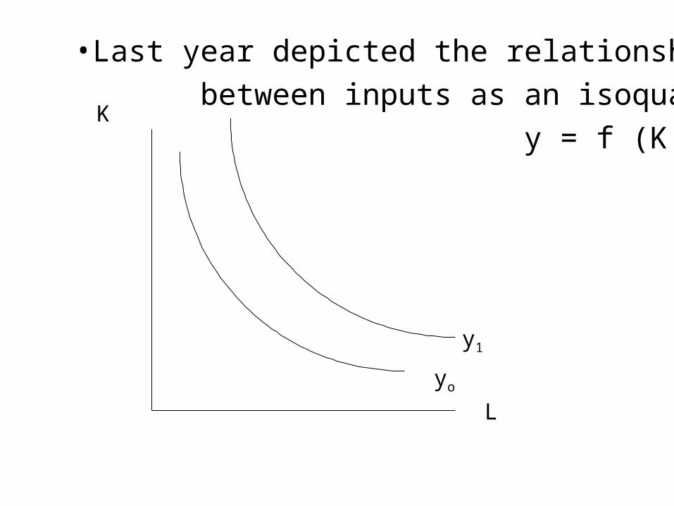
•Last year depicted the relationship

between inputs as an isoquant

y = f (K, L)K

L

yo

y1

L

K

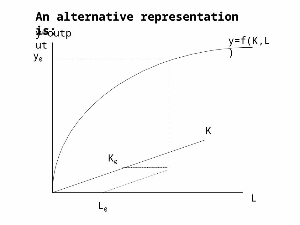
y=output

y0

L0

K0

y=f(K,L)

An alternative representation is:

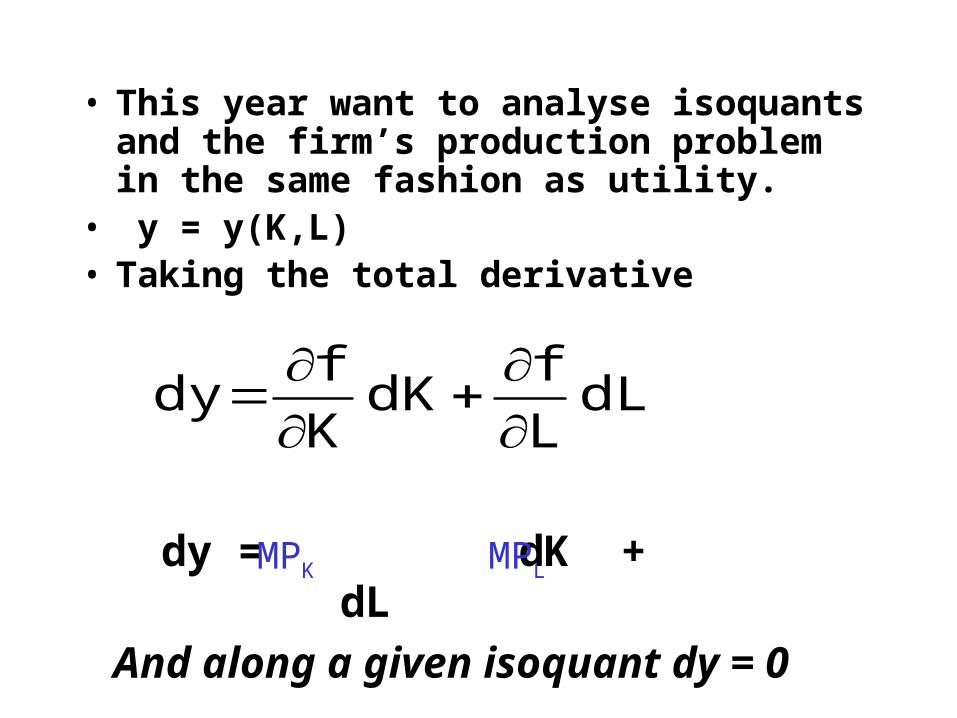
• This year want to analyse isoquants and the firm’s production problem in the same fashion as utility.

• y = y(K,L)• Taking the total derivative

dL L

fdK

K

fdy

dy = dK + dLMPK MPL

And along a given isoquant dy = 0

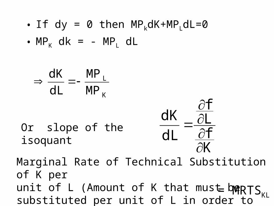
• If dy = 0 then MPkdK+MPLdL=0

• MPK dk = - MPL dL

K

L

MP

MP

dL

dK

KfLf

dL

dK

Or slope of the isoquant

Marginal Rate of Technical Substitution of K per unit of L (Amount of K that must be substituted per unit of L in order to keep output constant)

= MRTSKL

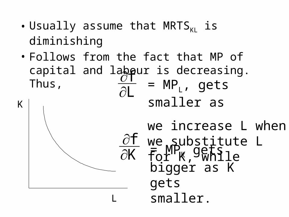
• Usually assume that MRTSKL is diminishing

• Follows from the fact that MP of capital and labour is decreasing. Thus,

K

L

Lf

= MPL, gets smaller as

we increase L when we substitute L for K, while

Kf

= MPk gets bigger as K gets smaller.

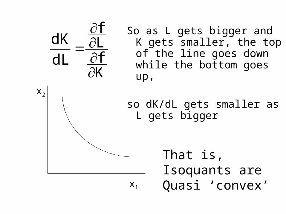
So as L gets bigger and K gets smaller, the top of the line goes down while the bottom goes up,

so dK/dL gets smaller as L gets bigger

That is, Isoquants are Quasi ‘convex’

x2

x1

KfLf

dL

dK

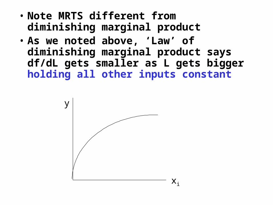
• Note MRTS different from diminishing marginal product

• As we noted above, ‘Law’ of diminishing marginal product says df/dL gets smaller as L gets bigger holding all other inputs constant

y

xi

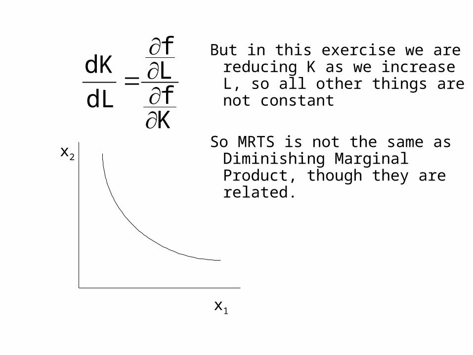
But in this exercise we are reducing K as we increase L, so all other things are not constant

So MRTS is not the same as Diminishing Marginal Product, though they are related.

x2

x1

KfLf

dL

dK

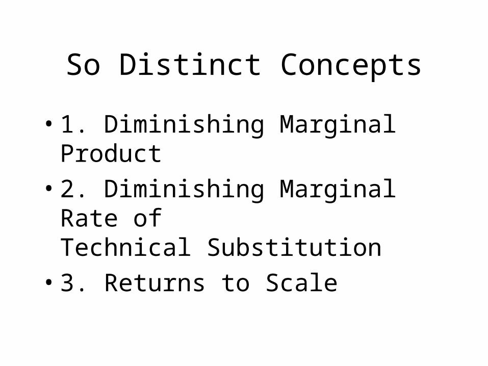
So Distinct Concepts

• 1. Diminishing Marginal Product

• 2. Diminishing Marginal Rate of … …Technical Substitution

• 3. Returns to Scale

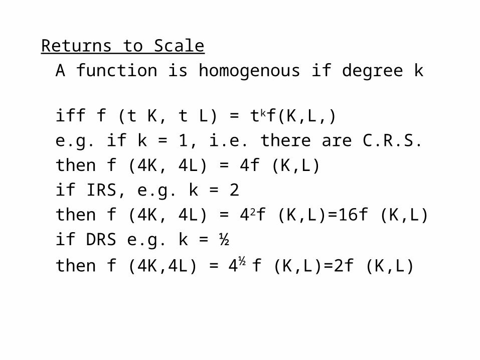
Returns to Scale

A function is homogenous if degree k

iff f (t K, t L) = tkf(K,L,)

e.g. if k = 1, i.e. there are C.R.S.

then f (4K, 4L) = 4f (K,L)

if IRS, e.g. k = 2

then f (4K, 4L) = 42f (K,L)=16f (K,L)

if DRS e.g. k = ½

then f (4K,4L) = 4½ f (K,L)=2f (K,L)

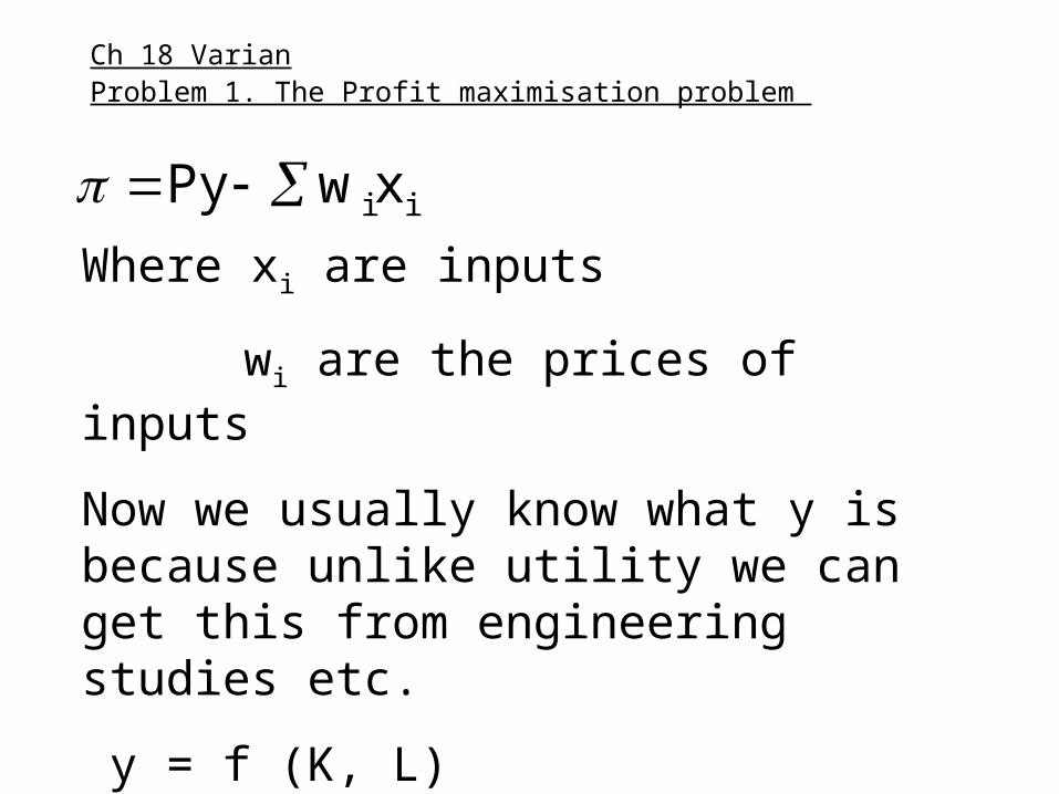
Ch 18 VarianProblem 1. The Profit maximisation problem

iixwPy Where xi are inputs

wi are the prices of inputs

Now we usually know what y is because unlike utility we can get this from engineering studies etc.

y = f (K, L)

Max w.r.t.K,L = P f (K, L) - rK - wL

wL

fP

L

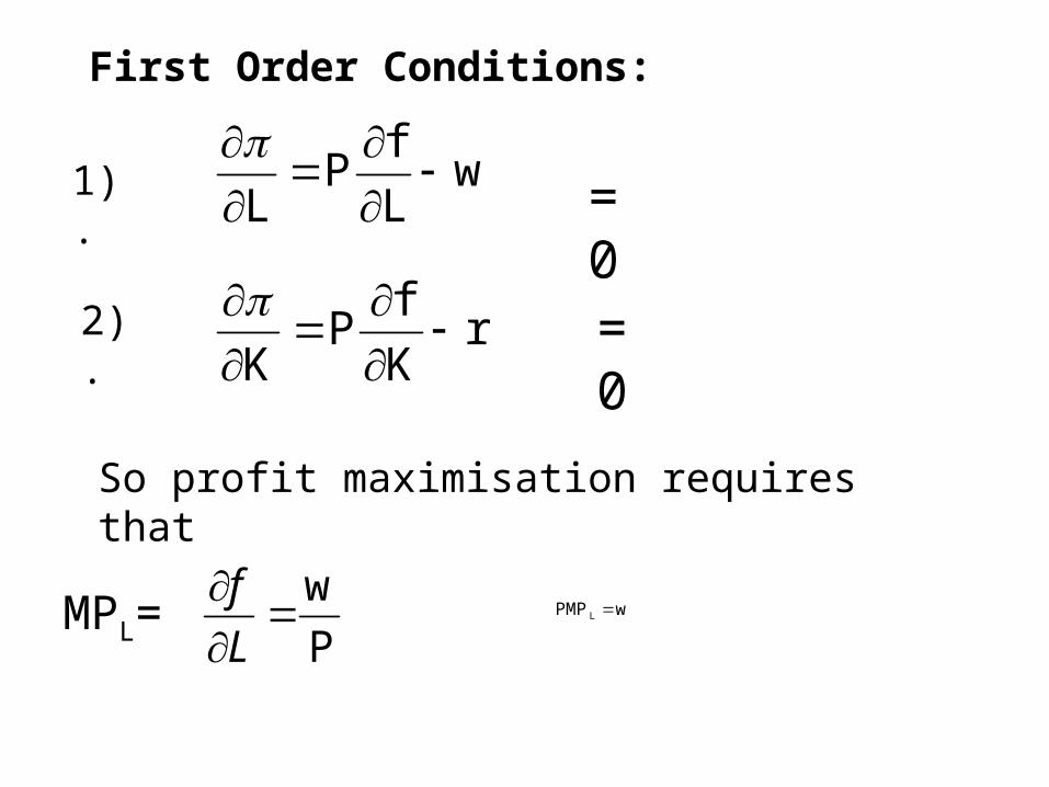
1).

2). rK

fP

K

So profit maximisation requires that

P

w

L

fwPMPL

= 0

= 0

First Order Conditions:

MPL=

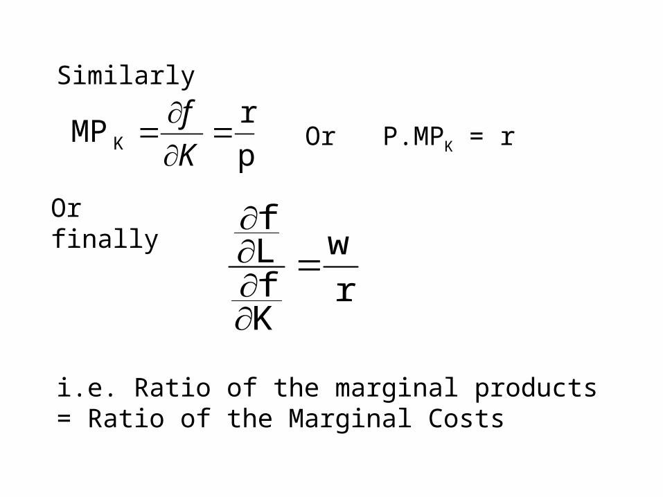
Similarly

p

rMPK

K

fOr P.MPK = r

Or finally

r

w

KfLf

i.e. Ratio of the marginal products = Ratio of the Marginal Costs

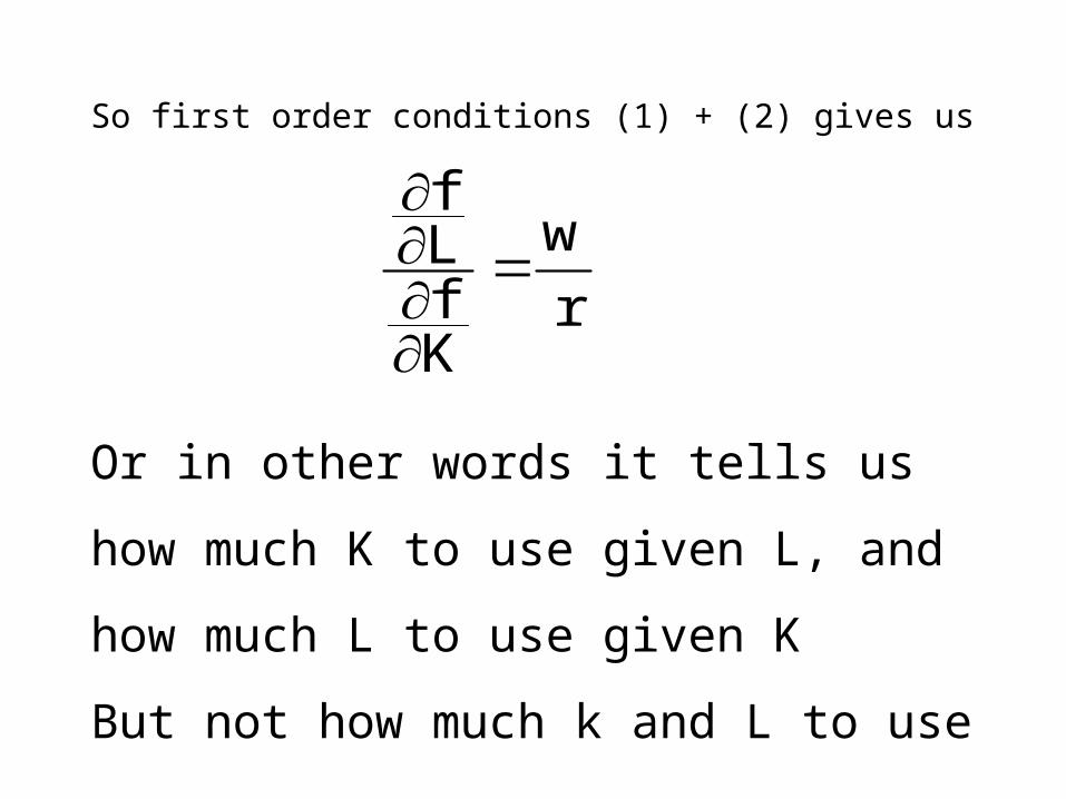
So first order conditions (1) + (2) gives us

r

w

KfLf

Or in other words it tells us

how much K to use given L, and

how much L to use given K

But not how much k and L to use

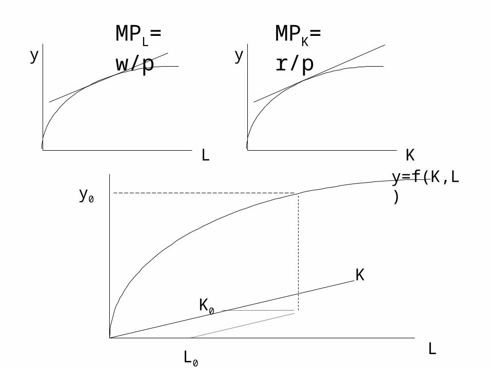
y

L

MPL= w/py

K

MPK= r/p

L

K

y0

L0

K0

y=f(K,L)

L

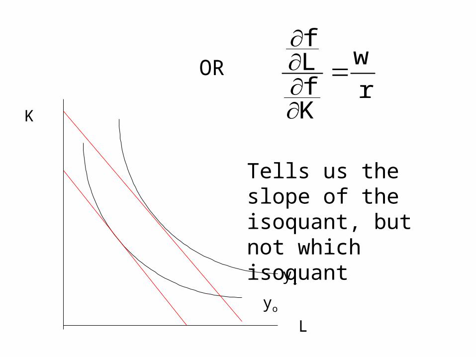
r

w

KfLf

OR

Tells us the slope of the isoquant, but not which isoquant

K

yo

y1

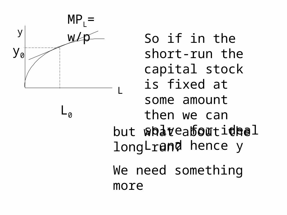
So if in the short-run the capital stock is fixed at some amount then we can solve for ideal L and hence y

y

L

MPL= w/p

L0

y0

but what about the long run?

We need something more

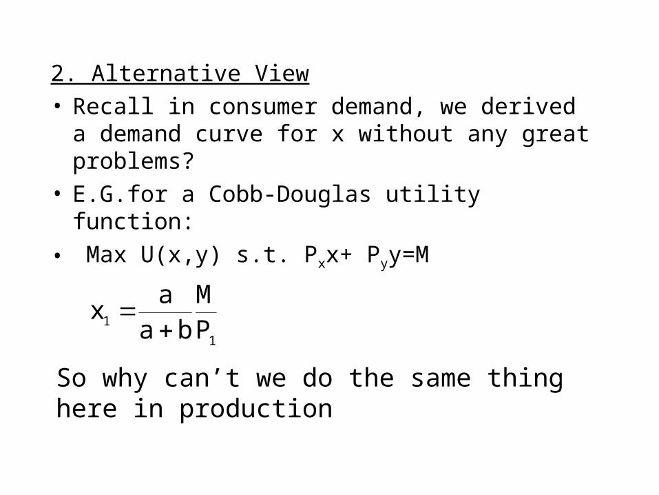
2. Alternative View• Recall in consumer demand, we derived a

demand curve for x without any great problems?

• E.G.for a Cobb-Douglas utility function:

• Max U(x,y) s.t. Pxx+ Pyy=M

1

1 PM

baa

x

So why can’t we do the same thing here in production

Profit Maximisation Problem 2

• Appendix to Ch 18

• An alternative to first problem

• Maximising output subject to a cost constraint

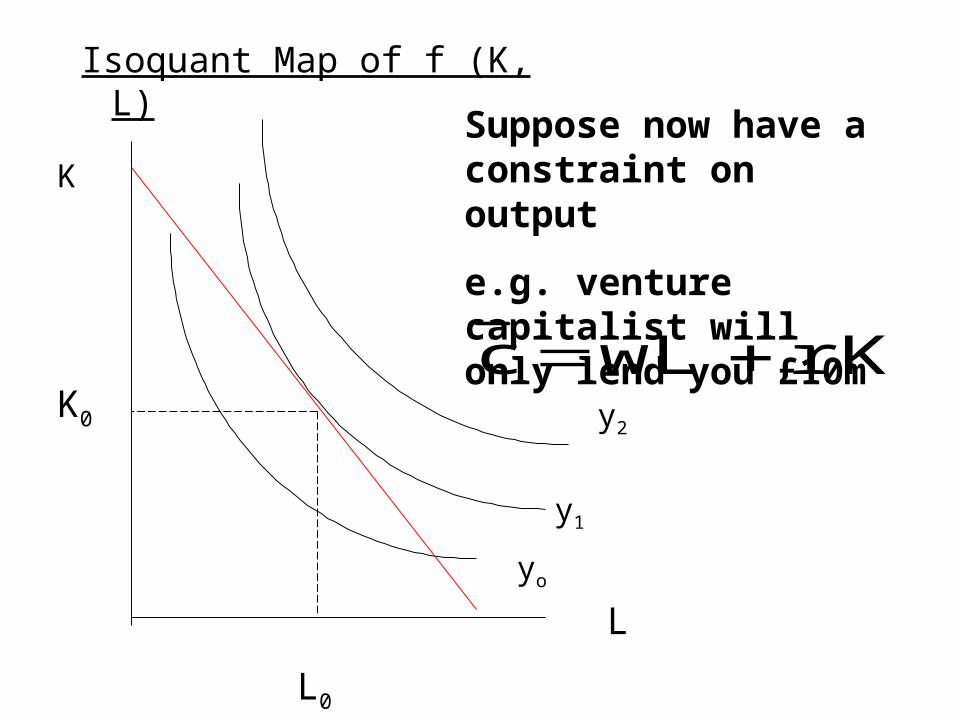
Isoquant Map of f (K, L)

rKwLc

Suppose now have a constraint on output

e.g. venture capitalist will only lend you £10m

K

yo

y1

L

y2

L0

K0

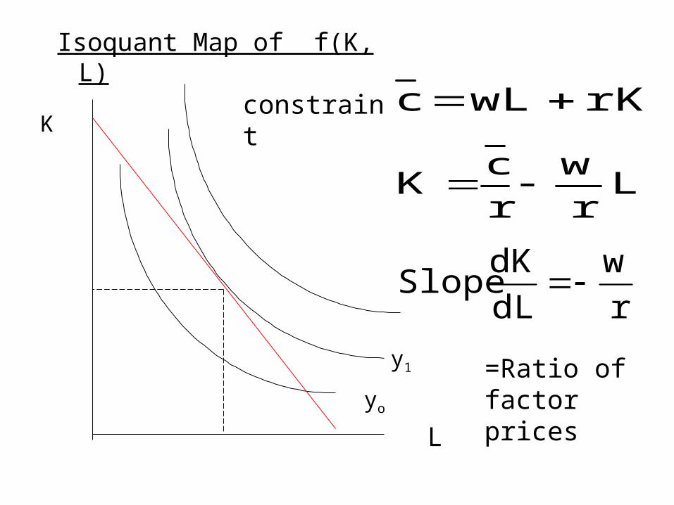
r

w

dL

dK Slope

Isoquant Map of f(K, L)

rKwLc

=Ratio of factor prices

constraintK

yo

y1

L

Lr

w

r

c K

Profit Maximisation Problem 3

• Varian Appendix Ch19

• Alternative to the Alternative in problem 2

• Minimising Cost subject to an Output constraint

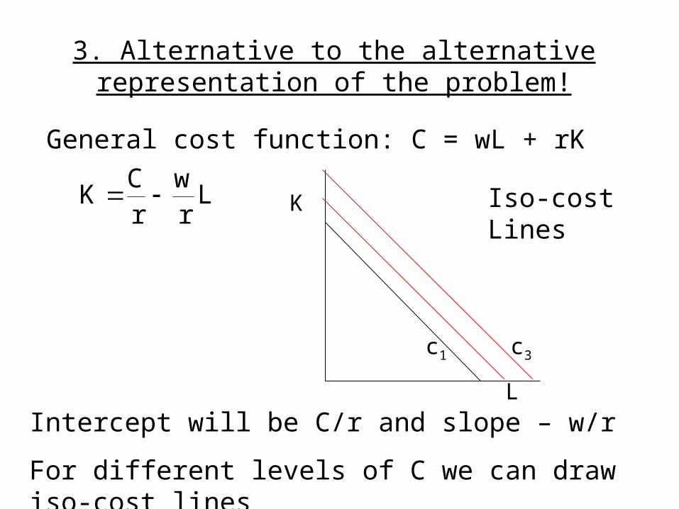
3. Alternative to the alternative representation of the problem!

General cost function: C = wL + rK

Lrw

rC

K K

L

c1

Iso-cost Lines

Intercept will be C/r and slope – w/r

For different levels of C we can draw iso-cost lines

c3

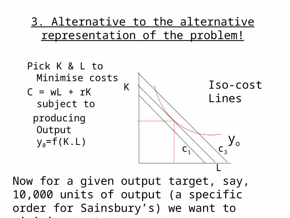
3. Alternative to the alternative representation of the problem!

K

L

c1

Iso-cost Lines

Now for a given output target, say, 10,000 units of output (a specific order for Sainsbury’s) we want to minimise costs.

c3

yo

Pick K & L to Minimise costs

C = wL + rK subject to

producing Output y0=f(K.L)

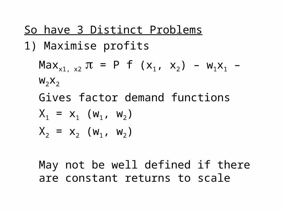
So have 3 Distinct Problems

1) Maximise profits

Maxx1, x2 = P f (x1, x2) – w1x1 – w2x2

Gives factor demand functions

X1 = x1 (w1, w2)

X2 = x2 (w1, w2)

May not be well defined if there are constant returns to scale

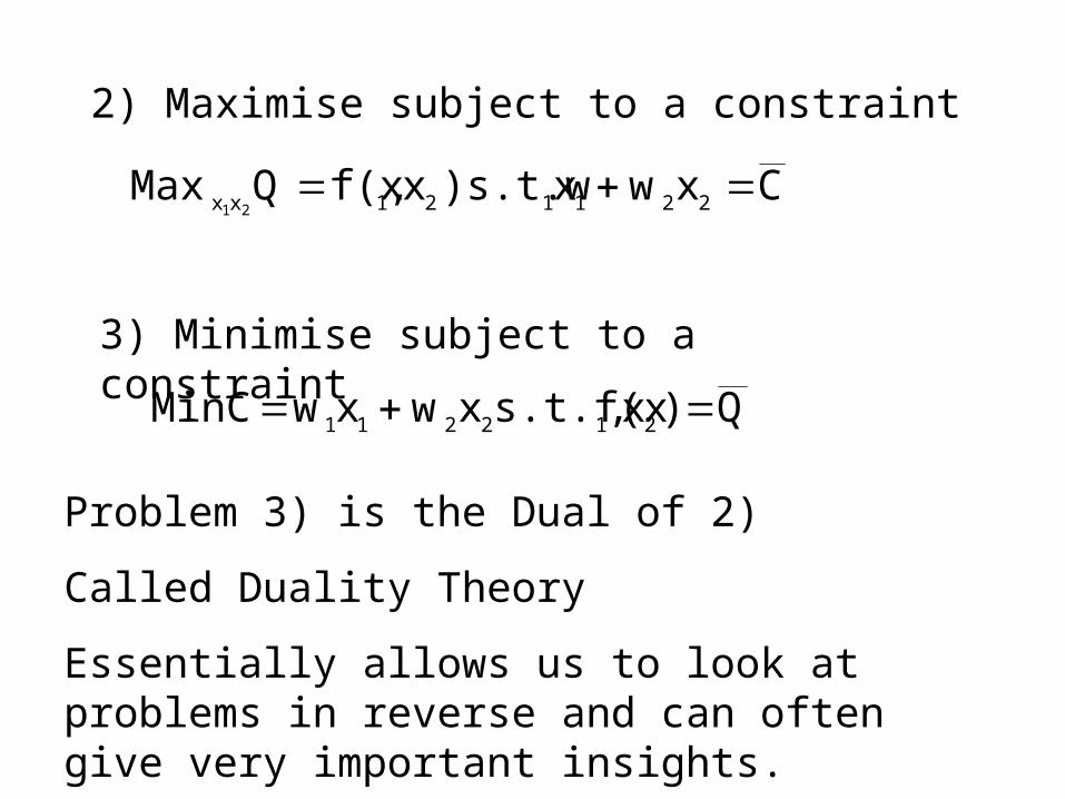
2) Maximise subject to a constraint

Cxwx)s.t.wx,f(xQMax 221121xx 21

3) Minimise subject to a constraint

Q)x,s.t.f(xxwxwMinC 212211

Problem 3) is the Dual of 2)

Called Duality Theory

Essentially allows us to look at problems in reverse and can often give very important insights.

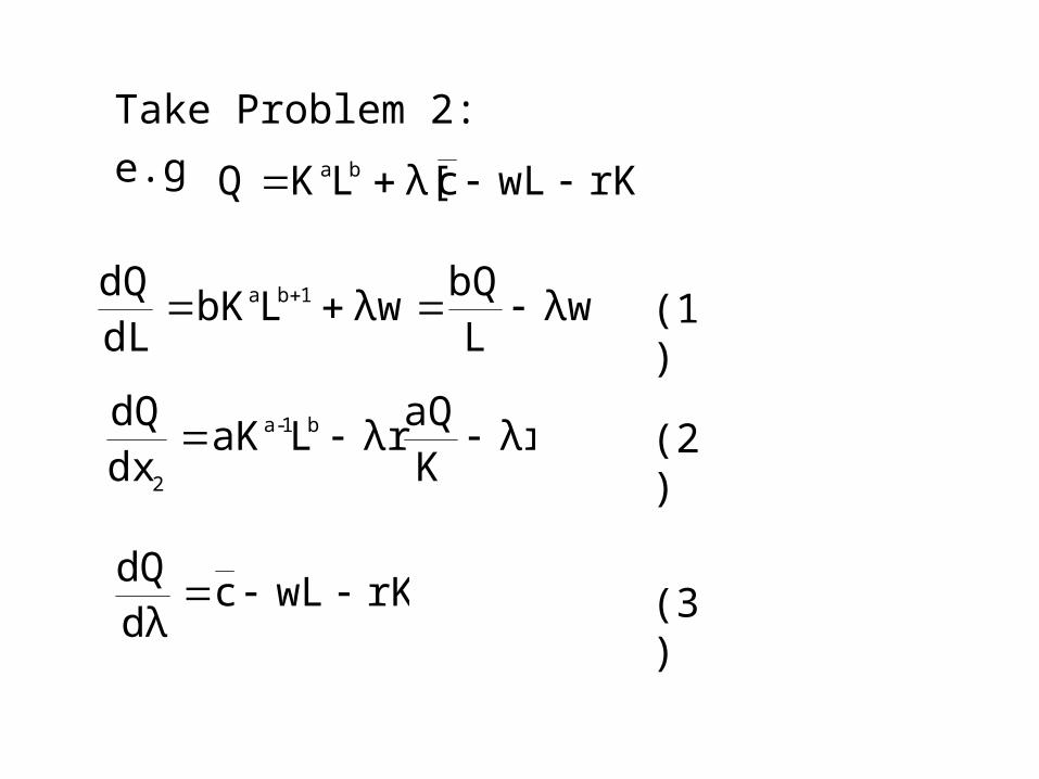
Take Problem 2:

e.g rK]wLcλ[LKQ ba

λwL

bQλwLbK

dLdQ 1ba (1)

λrK

aQλrLaK

dxdQ b1-a

2

(2)

rKwLcdλdQ (3)

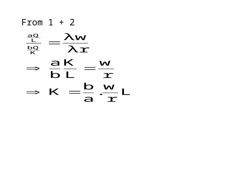
From 1 + 2

Lrw

.ab

K

rw

LK

ba

λrλw

KbQ

LaQ

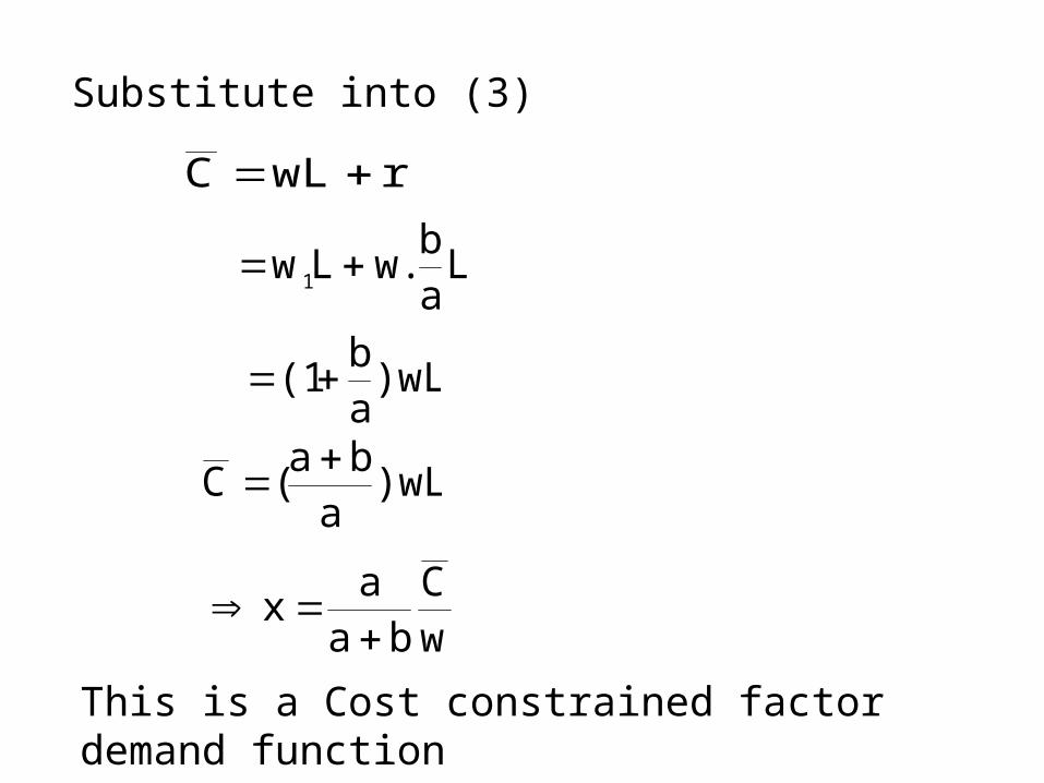
Substitute into (3)

r[wLC

Lab

w.Lw1

)wLab

(1

)wLa

ba(C

wC

baa

x

This is a Cost constrained factor demand function

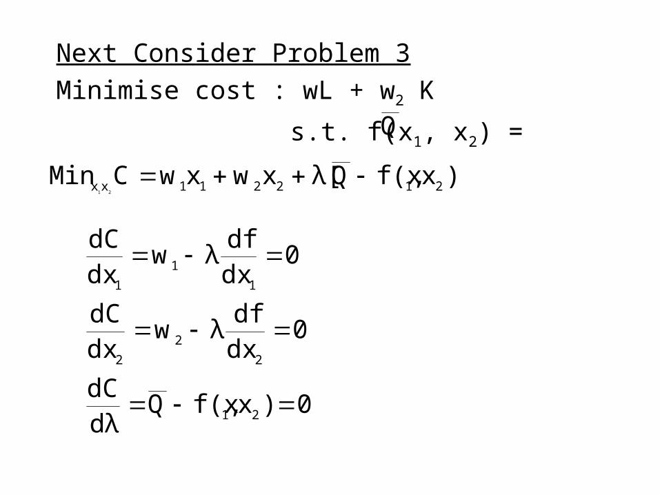
Next Consider Problem 3

Minimise cost : wL + w2 K

s.t. f(x1, x2) =Q

)]x,f(xQλ[xwxwCMin 212211xx21

0)x,f(xQdλdC

0dxdf

λwdxdC

0dxdf

λwdxdC

21

2

2

2

1

1

1

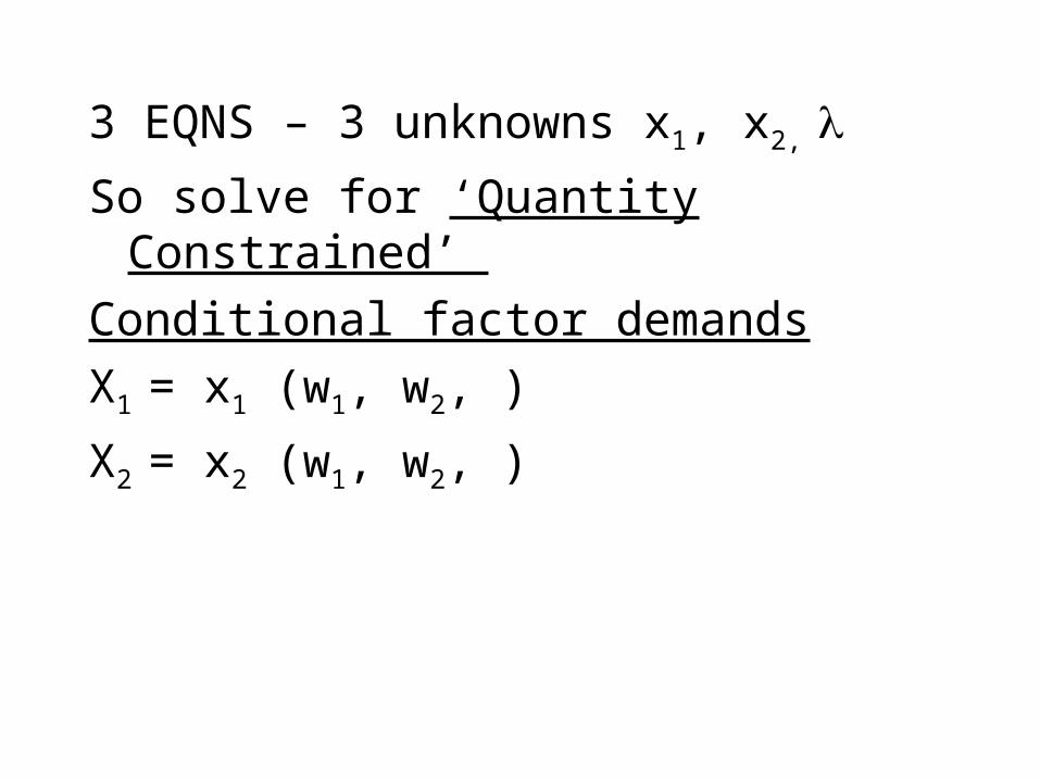
3 EQNS – 3 unknowns x1, x2,

So solve for ‘Quantity Constrained’

Conditional factor demands

X1 = x1 (w1, w2, )

X2 = x2 (w1, w2, )

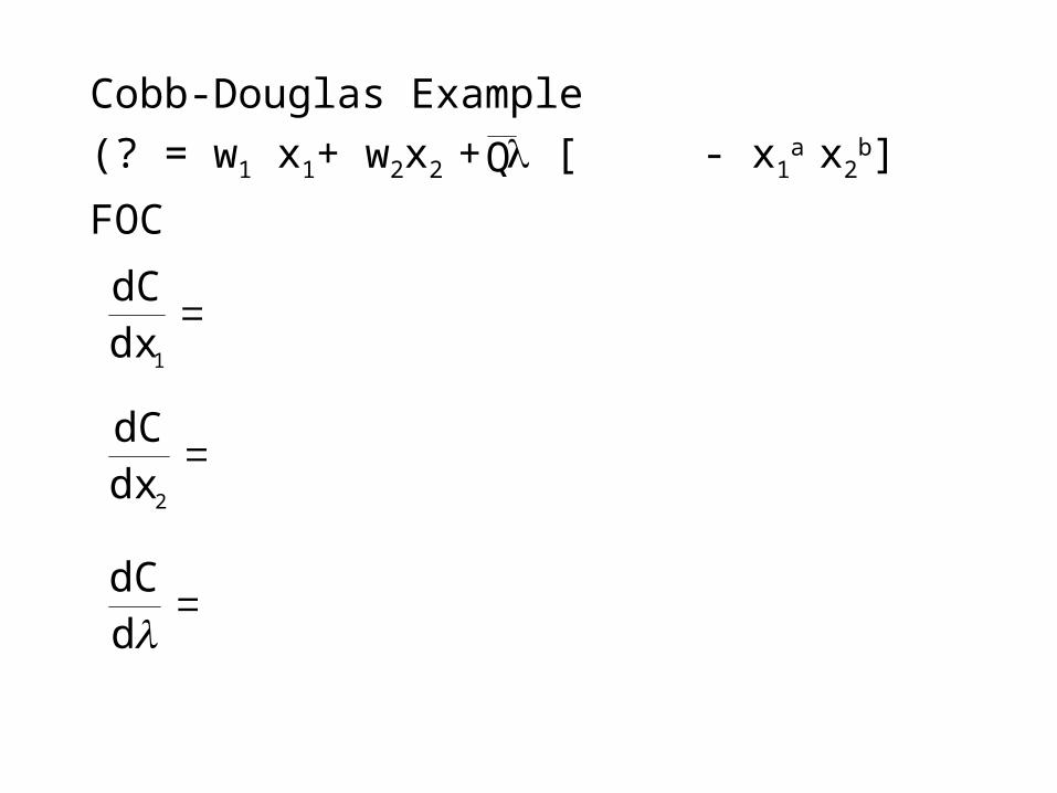
Cobb-Douglas Example

(? = w1 x1+ w2x2 + [ - x1a x2

b]

FOC

Q

1dx

dC

2dx

dC

d

dC

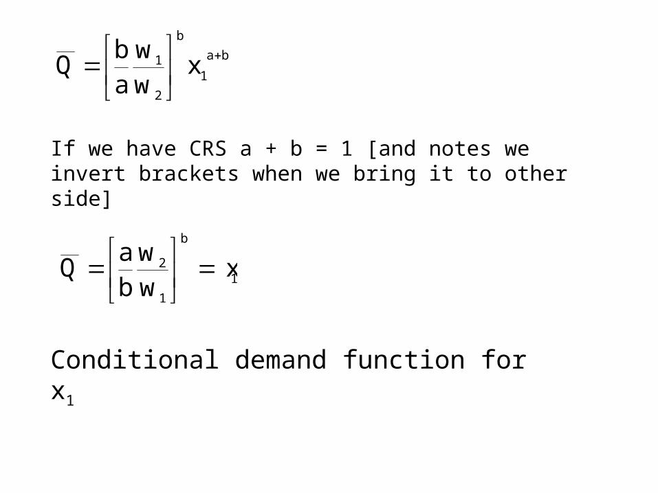
If we have CRS a + b = 1 [and notes we invert brackets when we bring it to other side]

ba

1

b

2

1 xww

ab

Q

1

b

1

2 xww

ba

Q

Conditional demand function for x1

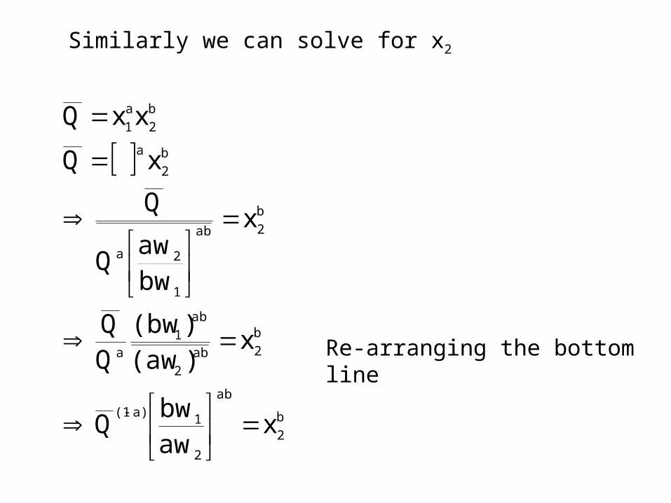
Similarly we can solve for x2

b

2

ab

2

1a)(1

b

2ab

2

ab

1a

b

2ab

1

2a

b

2

a

b

2

a

1

xawbw

Q

x)(aw)(bw

QQ

x

bwaw

Q

Q

xQ

xxQ

Re-arranging the bottom line

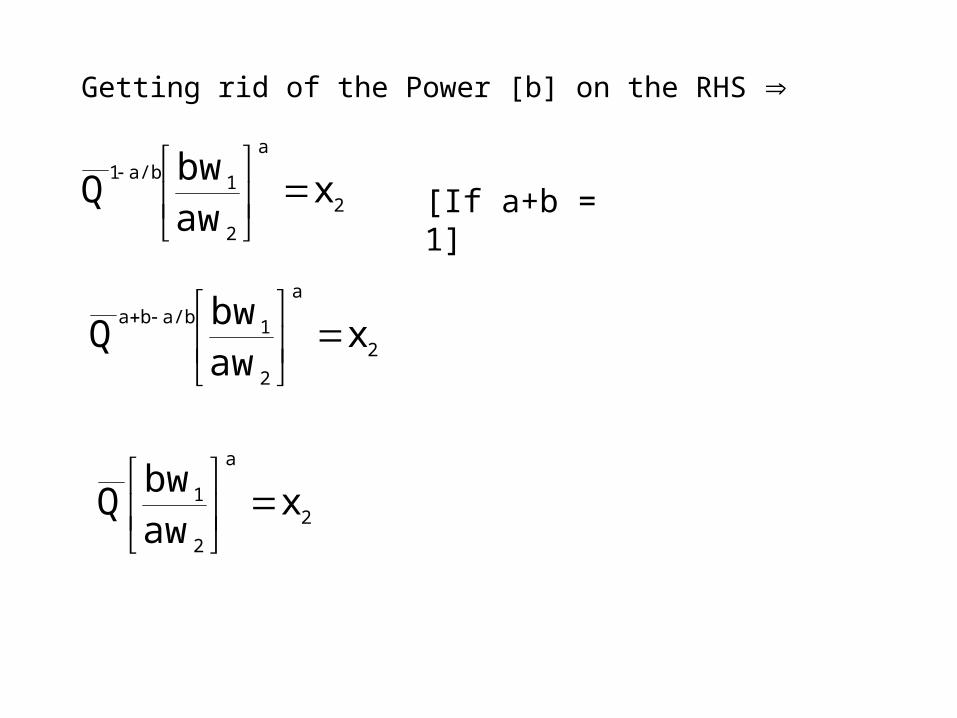
Getting rid of the Power [b] on the RHS

2

a

2

1a/b1x

awbw

Q

2

a

2

1a/bbax

awbw

Q

2

a

2

1 xawbw

Q

[If a+b = 1]

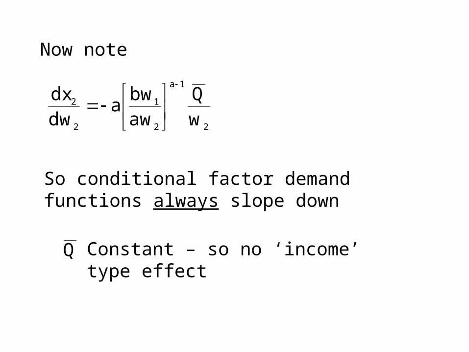
Now note

2

1a

2

1

2

2

wQ

awbw

adwdx

So conditional factor demand functions always slope down

Q Constant – so no ‘income’ type effect

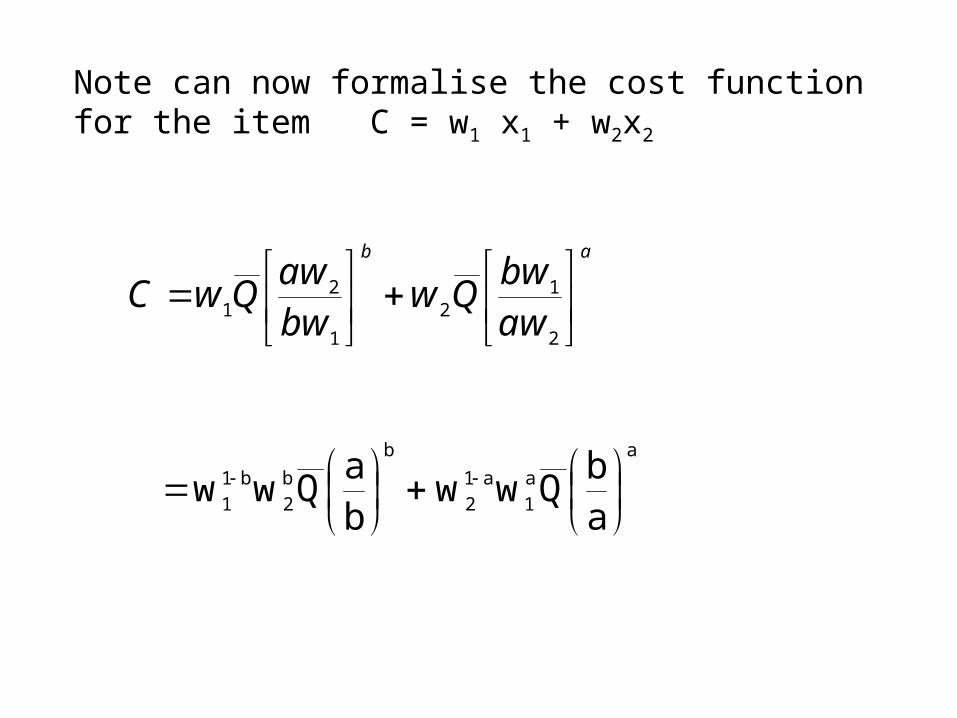
Note can now formalise the cost function for the item C = w1 x1 + w2x2

ab

awbw

Qwbwaw

QwC

2

12

1

21

a

a

1

a1

2

b

b

2

b1

1 ab

Qwwba

Qww

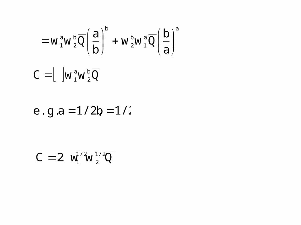
a

a

1

b

2

b

b

2

a

1 ab

Qwwba

Qww

Qww C b

2

a

1

Qw w2 C 1/2

2

1/2

1

1/2b1/2,a e.g.