Embed Size (px)
Citation preview
PRODUCTION ORGANIZATION AND EFFICIENCY DURING TRANSITION:AN EMPIRICAL ANALYSIS OF EAST GERMAN AGRICULTURE
Erik Mathijs and Johan F. M. Swinnen
Policy Research GroupWorking Paper
No. 7
May 1997
ABSTRACT
Farm restructuring is expected to improve efficiency in transition economies. With data fromformer East Germany we compare the efficiency of family farms and partnerships with large-scale successor organizations of the collective and state farms (LSOs). Our efficiencyanalysis, using parametric and non-parametric techniques, shows that LSOs display lowertechnical efficiency than family farms and partnerships, but that this difference is small anddeclining during transition, mainly as a result of structural changes in agriculture. Familyfarms are less scale efficient than partnerships and LSOs. Partnerships are superior to allother organizational forms regardless of the measuring technique used.
JEL Classification Numbers: O47, P5, P15, Q16.
The authors acknowledge financial support of the Belgian National Foundation for ScientificResearch (NFWO) and thank Volker Beckmann, Konrad Hagedorn, Jozef Konings, KarenMacours, Erik Schokkaert and participants at seminars in Leuven and Rome (FAO) for helpfulcomments and assistance.
Policy Research Group, Department of Agricultural Economics, Katholieke UniversiteitLeuven, Kardinaal Mercierlaan 92, 3001 Leuven, Belgium, Tel.: ++32 16 321618 - Fax: ++ 3216 31996 - E-mail: [email protected]
1
PRODUCTION ORGANIZATION AND EFFICIENCY DURING TRANSITION:AN EMPIRICAL ANALYSIS OF EAST GERMAN AGRICULTURE
I. INTRODUCTION
An important issue in the economic transition in Central Europe is the restructuring of
production organizations and its impact on productivity and efficiency. A key issue in the
literature is whether so-called de novo firms will be more efficient than restructured former
state and collective enterprises facing hard budget constraints in a competitive environment.1
In agricultural production, these de novo firms are typically family farms or small associations
of family farms. The former collective and state farms which have not been liquidated, have
typically been transformed into either a “private cooperative” or a joint stock company
(Swinnen, Buckwell and Mathijs, 1997). We will refer to both organizations as “large-scale
successor organizations” (LSOs).
Two factors have an important – and opposite – effect on the relative efficiency of these
various organizations in agricultural production: labor transaction costs and scale economies.
First, LSOs are expected to display lower levels of technical efficiency because of their
inherent problems in solving principal-agent problems in labor contracting related to the
difficulties of linking effort in production to income (Schmitt, 1993). As a result, individuals in
these production organizations have more incentive to shirk. This problem is due to the
difficulty of metering effort in production (Alchian and Demsetz, 1972) – which is particularly
stringent in agriculture because of its biological and sequential nature and spatial dimensions
(e.g., Brewster, 1950; Binswanger and Rosenzweig, 1986). Family farms are more efficient in
this regard because family members maximize family welfare rather than individual welfare and
hence face no incentive to free ride, so that the costs of monitoring and controlling labor effort
are lower (Carter, 1984). Based on these theoretical observations – and the domination of
family farms in most OECD countries’ agriculture – several authors have concluded that family
farms are superior organizations in agricultural production (Pollak, 1985; Schmitt, 1991).
Second, scale economies would favor the largest organizations. However, many studies
suggest that there are no increasing returns to farm size in production beyond what can be
captured by the family farm both in developing (Berry and Cline, 1979; Hayami and Ruttan,
1 See for example the special issue of the Journal of Comparative Economics edited by Ben-Ner, Brada andNeuberger (1993) for a comprehensive overview of the issues and Brada, King and Ma (1997) for an analysis ofenterprise efficiency in Hungary and the Czech Republic.

2
1985) and in developed countries (Kislev and Peterson, 1991; Peterson, 1997). Advantages of
cooperation and economies of scale do exist in output marketing, input purchasing, credit and
information provision and risk management. In many countries these scale economies are
captured by marketing and credit cooperatives. However, in a transition economy where
cooperative frameworks limited to input purchasing, credit negotiation and output marketing
are typically absent, these ‘intrinsic’ scale advantages may provide important advantages to
LSOs and may offset their transaction cost disadvantages, at least during the transition period
(Carter, 1987; Machnes and Schnytzer, 1993; Deininger, 1995). Moreover, some argue that
state and collective farms performed poorly not because of their intrinsic problems, but
because of extrinsic problems, such as bureaucratic controls and extractive external
environments (Johnson, 1983; Putterman, 1985). This result would imply that LSOs will be
able to survive and compete as production organizations even after the transition is over.
Empirical evidence on the relative efficiency of large-scale (sometimes cooperative) and
small-scale (mostly family farms) organizations is rather scarce and is limited to earlier reforms
in socialist countries in East Asia and to pre-reform comparisons in those Central European
countries where private farms were important during Communism. The studies show that
institutional reform had a large positive impact on agricultural growth in China (McMillan et
al., 1989; Lin, 1992) and in Vietnam (Pingali and Xuan, 1992). Evidence for Central Europe is
limited to pre-1989 comparisons of small-scale family farms and large-scale collective (or
state) farms in Poland and Yugoslavia. Boyd (1987a,b) shows that both in Poland and
Yugoslavia there is no difference in technical efficiency between state farms and private farms.
Improved techniques based on frontier estimates yield ambiguous results: they confirm Boyd’s
results for Poland (Brada and King, 1993), but Hofler and Payne (1993) reject them for
Yugoslavia. Brada and King conclude that indeed “it is the environment of socialized
agriculture rather than the socialized nature of farms that leads to the poor performance of the
agricultural sector in Eastern Europe and the former Soviet Union” (p. 54).
However, all these studies suffer from two important remaining methodological flaws.
First, since they all use parametric estimation techniques, their results are highly sensitive to the
specified functional form of the production function. Second, parametric estimations do not
allow to estimate the scale efficiency of organizations. The use of non-parametric techniques
to calculate technical and scale efficiency therefore provides useful complementary
information. For example, Piesse, Thirtle and Turk (1996) complement their parametric
estimations with non-parametric calculations to show that in the Slovenian dairy sector private

3
farms display higher technical efficiency but lower scale efficiency than cooperatives.
Unfortunately, their analysis is limited to the period 1974-1990. Post-reform efficiency studies
are still unavailable, mainly due to the absence of reliable and consistent data on the
performance of different organizational forms in Central European agriculture since 1989.
This paper presents the first analysis – to our knowledge – of differences in efficiency
between different farm organizations after the 1989 reforms in Central Europe.2 East German
data are used since German statistics are the most consistent and reliable in a former
Communist economy presently available. Our analysis shows that in former East Germany,
LSOs display lower levels of technical efficiency than partnerships and family farms, but that
this difference is small and declining during transition. Our results also indicate that family
farms are less scale efficient than both partnerships and LSOs, and that farms organized as
partnerships are the most efficient organizational form regardless of the measuring technique
used. Because of the unique conditions of East German agriculture as a result of the
unification and the subsequent integration into the Common Agricultural Policy of the
European Union, one should be cautious to generalize any findings based on the East German
experience to other transition economies.
The paper is organized as follows. Section 2 presents the data used for the empirical
analysis. While technical efficiency is estimated using parametric efficiency measures in section
3, non-parametric measures of technical and scale efficiency are calculated in section 4. The
results of these calculations are tested in a fifth section. Section 6 discusses the results and
formulates some hypotheses. Section 7 concludes the paper.
II. DATA
Data for the analyses are taken from the official German statistics on annual production and
input use by three farm categories from 1991/92 to 1994/95 and are averages of panel data
(Agrarbericht, 1996). Data are also available according to farm specialization (crops or
livestock). All calculations are based on a single aggregate output and three conventional
inputs: land, labor and capital. As a proxy for production, we use agricultural output, Y, i.e.
the production value in German Marks (DEM) deflated by the consumer price index (OECD,
2 Many qualitative and theoretical analyses are available. For former East Germany, see e.g. the debatebetween Peter and Weikard (1993) and Beckmann, Schmitt and Schulz-Greve (1993) on the relative efficiency

4
1996). LAND is cultivated land in hectares. LABOR is the number of annual work units
(‘Arbeitskräfte’). CAPITAL is the sum of the value of buildings, machinery and livestock in
DEM deflated by the consumer price index.3
Table 1 displays the relative importance of each of these organizations and their average
size in terms of cultivated land in East Germany during transition. Table 2 summarizes the
descriptive statistics of the sample which is used for our analysis.
1. Family farms (‘Einzelunternehmen’). The category of family farms, or ‘sole proprietors’,
includes farms worked and managed by a single household. The economic size of the farms
varies from less than 40,000 DEM to more than 100,000 DEM Standard Farm Income
(‘Standardbetriebseinkommen’). The importance of these family farms increased from 13
percent of total cultivated land in 1992 to 21 percent in 1995. The average size of the farms
in the sample is 199 ha for crop farms and 81 ha for farms specialized in animal products
and is higher than the average size of the population (45-48 ha). On average, family farms
in the sample employ between 1.4 and 2.8 labor units.
2. Partnerships (‘Personengesellschaften’). Most partnerships were established as new
enterprises (Beckmann and Hagedorn, 1997). They typically result from the collaboration
of only a few people (they employ about 5 labor units on average) which in many cases are
family related. Partnerships differ from companies and cooperatives because they have
unlimited liability (as do family farms). The main reason of their establishment was to
overcome the difficulties single family farms face in getting access to credit given increasing
capital needs (Welschof, 1995).4 Their evolution is parallel with that of family farms.
Partnerships covered 14 percent of total cultivated land in 1992 and 22 percent in 1995.
The partnerships in the sample have on average 250-534 ha of land, which is comparable in
size to the overall average.
3. Legal entities (‘juristische Personen’). This category includes both farms organized as
cooperatives and as joint stock companies. Both types of farms are characterized by limited
of production organizations. Beckmann and Hagedorn (1997) provide a more general overview of structuralchange in East German agriculture.3 Since output and capital are expressed in monetary terms, our results may be sensitive to differences betweenfamily farms and LSOs in how assets are valued and how they react to policy changes.4 For example, dairy farms face high capital needs to finance the purchase of milk quota.
5
liability. Most of these farms were created from former cooperative farms – the so-called
‘Landwirtschaftliche Produktionsgenossenschaften’ (LPGs) – whereas the majority of
partnerships were established as new enterprises. We refer to this category as large-scale
successor organizations (LSOs) of the LPGs. The data do not allow disaggregation
between companies and cooperatives, such that our conclusions will apply to LSOs in
general. Both companies and cooperatives are transformed LPGs. In fact, 40 percent of
the LPGs have been eliminated, whereas 60 percent has been transformed into one of the
legal forms provided by West German Law. Out of the 60 percent of LPGs that have not
been liquidated by 1992, 49 percent were transformed into cooperatives, 41 percent into
companies and 13 percent into partnerships (Beckmann and Hagedorn, 1997). The share of
LSOs in total cultivated land decreased steadily from 73 percent in 1992 to 57 percent in
1995. The average size of LSOs in the sample exceeds that of the population considerably.
Moreover, it must be indicated that cooperatives are generally larger than companies. LSOs
employ about 50 labor units on average.
III. ESTIMATING TECHNICAL EFFICIENCY USING PARAMETRIC METHODS
Frontier estimation
A production organization is technically efficient if it produces on the boundary of the
production possibilities set, that is, it maximizes output with given inputs and after having
chosen technology. This boundary or frontier is defined as the best practice observed within
the sample. Deviations from the frontier reflect the intensity of resource use, i.e. since
production inputs are not measured in technical productivity units and effort determines both
labor productivity and the intensity and intelligence with which non-labor inputs are used, any
variation in the intensity and effort with which firms utilise observed inputs, are reflected in
variation in technical efficiency (Carter, 1984, p. 830).
We will analyze the technical efficiency of different organizations by comparing the
observed output of a certain activity k5, Yk, produced using land, labor and capital, to an
‘efficient’ output level, ~Y k, located on the frontier production function. This frontier contains
5 Activities can be different farms at a certain point of time, a particular farm at different points in time, or acombination of both.

6
the maximum output levels given certain input bundles. The ratio of observed output to
efficient output is then the level of technical efficiency for activity k, ek = Yk/~Y k. We will first
estimate this frontier in a standard, parametric way. More specifically, following Lin (1992),
Hofler and Payne (1993), Piesse, Thirtle and Turk (1996) we use a Cobb-Douglas
specification, because the available data do not contain sufficient information to permit the
estimation of more sophisticated functional forms. The estimates thus derived are the so-called
Timmer measures of technical efficiency.6
The production function frontier can be either stochastic – i.e. the frontier can be subject to
statistical noise – or deterministic – i.e. the frontier is fixed. We will first investigate whether
to use a stochastic or a deterministic frontier for the efficiency estimation. The stochastic
frontier can be written as follows:
(1) ln(~Y ) = ~α 1 + ~α 2 T92/93 + ~α 3 T93/94 + ~α 4 T94/95+
~βA ln(LAND)
+ ~βL ln(LABOR) +
~βK ln(CAPITAL) + ~v - ~u
where ~α 1 denotes the intercept for 1991/92; the T’s are dummy variables for each year (1 for
that year, 0 for other years), and the ~β ’s are the production elasticities at the frontier. The
time dummies are included to account for yearly shifts of the frontier. The error term is
decomposed into a two-sided error term which is normally distributed, ~v ~ N(0, σ v2 ), and
represents statistical noise, and a one-sided error term ~u ≥ 0 which follows a half-normal
distribution with mean µ and variance σ u2 and represents technical inefficiency. The stochastic
frontier is estimated using the maximum likelihood technique of LIMDEP following Aichner,
Lovell and Schmidt (1987).
Excluding statistical noise from specification (1) yields the deterministic frontier:
(2) ln(~Y ’) = ~α 1 ’+ ~α 2 ’ T92/93 + ~α 3 ’T93/94 + ~α 4 ’ T94/95 +
~βA ’ ln(LAND)
+ ~βL ’ ln(LABOR) +
~βK ’ ln(CAPITAL) - ~u ’
6 See Timmer (1971) for more detail.
7
where all coefficients and variables have the same interpretation as in (1), except for the error
term which contains only a one-sided negative error term ~u ’. We estimated the deterministic
frontier using corrected ordinary least squares (COLS) (Greene, 1980; Russel and Young,
1983; Piesse, Thirtle and Turk, 1996).7 It involves first the estimation of the average
production function, ln( Y ), which is characterized by an intercept α1, by means of OLS:
(3) ln( Y ) = α1 + α2 T92/93 + α3 T93/94 + α4 T94/95 + βA ln(LAND) + βL ln(LABOR)
+ βK ln(CAPITAL) + v
where the β’s are the production elasticities of the different inputs and v denotes statistical
noise. To yield the frontier the production function thus estimated is shifted upwards with
intercept ~α 1, so that the observation with the largest positive residual lies on the frontier:
(4) ln(~Y ) = ~α 1 + α2 T92/93 + α3 T93/94 + α4 T94/95 + βA ln(LAND) + βL ln(LABOR)
+ βK ln(CAPITAL),
that is, the new intercept equals ~α 1 = α1 + vmax where vmax is the largest positive error and is
considered to be the most efficient observation. This approach assumes that the slope
parameters of the average production function and the frontier are the same.
The results of both estimations are summarized in table 3. All coefficients are statistically
significant at the one percent level, except for the intercept and the coefficient for labor, which
is negative but does not differ significantly from zero. Table 3 suggests further that the
stochastic frontier does not differ significantly from the deterministic frontier. The variance of
the one-sided error term was much higher (0.016) than the variance of the two-sided error
term (2 10-10). Therefore, the results of the stochastic estimation hardly differ from the results
of the deterministic estimation. This is not surprising since we use average data. As both
approaches yield similar results, we calculate efficiency measures based on the deterministic
frontier. We also estimated the deterministic frontier without dummies for each year. The
estimated coefficients are presented in the last column of table 3. This approach yields a
positive coefficient for labor and will be used for the calculation of the efficiency measures.
7 Another method is to use programming techniques.

8
Any interpretation of efficiency measures will have to take into account that any shifts of the
frontier during transition will now show up in the efficiency estimations.
Efficiency calculation
Technical efficiency measures are calculated for the individual observations by subtracting the
largest positive residual from all residuals setting the error term of the most efficient
observation equal to zero. Exponentiation gives the relative efficiency of each observation as a
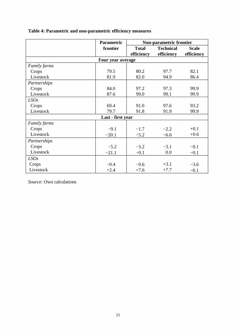
percentage of the most efficient one. The results of these calculations are in table 4.
In crop production, partnerships (84.0) turn out to be more efficient than family farms
(79.5) and LSOs (69.4). The same pattern can be observed in livestock production, albeit that
the difference between family farms (81.9) and LSOs (79.7) is much smaller now. In crop
production, technical efficiency decreases over time in all types of farms, but considerably
more in family farms (-9.1) and partnerships (-5.2) than in LSOs (-0.4). The differences are
greater in livestock production: technical efficiency of partnerships and family farms decreases
with about 20 percentage points, while LSOs show a slight increase in technical efficiency
(+2.4). Finally, it can be observed that the difference in technical efficiency between
partnerships and family farms on the one hand and LSOs on the other hand is greater in crop
production (+14.7 and +10.1 respectively) than in livestock production (+7.9 and +2.2
respectively).
Discussion
Some of these results are remarkable, but before trying to explain and interpret these results,
we discuss some problems with the model specifications and some methodological refinements
to improve and decompose the efficiency calculations.
The approach used for our estimations and efficiency calculations is the same as the one
used by Hofler and Payne (1993) and Piesse, Thirtle and Turk (1996). However, this approach
has two important problems. First, parametric analysis involves the choice of a specific
production function and using observable production behavior to estimate the underlying
parameters. In order not to impose a priori restrictions, flexible functional forms can be used
for estimation (e.g., quadratic, translog and generalized Leontief forms), but results are still
sensitive to the particular parametric functional form chosen. Moreover, the choice of a

9
particular functional form implies that one has a priori information on the actual form. Since
this kind of information is mostly absent, methods that do not rely on the strict parametric
assumptions are preferred (Chavas and Cox, 1995). Second, parametric estimations do not
allow the decomposition of total efficiency in technical and scale efficiency.
Two observations indicate the possibility of a misspecification of the production function:
first, the coefficient of labor is negative both for the stochastic and the deterministic estimation,
and second, the sum of coefficients is equal to 1.21 and 1.18 for the stochastic and the
deterministic frontier respectively, indicating that increasing returns to scale is the dominating
feature of the observations in the sample. Introducing a slope dummy in (3) for LSOs on the
coefficient for LAND considerably increases the coefficient for labor to 0.35, while decreasing
the other coefficients. The sum of coefficients is near 1 for LSOs, while it is still larger than 1
for family farms. These results indicate that there may exist more than one frontier and that
family farms display increasing returns to scale, while LSOs display constant returns to scale.
However, as pointed out by Brada and King (1993), the different coefficients thus estimated
may well reflect differences in input use, rather than differences in production technology.
Pooling tests based on asymptotic likelihood comparing restricted and unrestricted
specifications confirm that data for family farms and partnerships on the one hand and LSOs on
the other hand can be pooled.8 We thus share the view of Brada and King and have calculated
the efficiency measures based on a restricted specification. Nevertheless, because the sample is
dominated by family farms and partnerships (32 of the 44 observations), estimations will be
biased towards family farms and partnerships, such that the efficiency measures for LSOs is
likely to be underestimated. We will therefore use non-parametric calculations in the next
section to improve the measurement of technical efficiency and to calculate scale efficiency.
IV. ESTIMATING TECHNICAL AND SCALE EFFICIENCY USING
NON-PARAMETRIC METHODS
8 A test for pooling data involves the estimation of a restricted (no intercept and slope dummies) and anunrestricted production function and the calculation of the log-likelihood ratios of each specification. Thesignificance of the difference between the log-likelihood ratios can then be evaluated using the χ2-distribution.The χ2 statistics for introducing individual slope variables (5.24 for land, 3.86 for labor, 4.20 for capital and4.30 for the intercept) all lie between the critical χ2 values at the 95 and 99 percent confidence levels (3.84 and6.63, respectively).

10
A non-parametric test is not a statistical test, but checks a set of inequalities which guarantee
the existence of a production function that can rationalize a set of data in the context of the
hypothesis of some behavioral goal (in general, profit maximization or cost minimization). It
compares observed production behaviour with the situation that satisfies the producer’s
behavioral goal. The comparison can be made both in terms of quantities (inputs and outputs)
and values (revenue, profit and cost).
Methodology
As in Färe, Grosskopf and Lovell (1985), we assume that production is characterized by a non-
parametric piecewise-linear technology, so that simple linear programming techniques can be
used. We further assume strong disposability of outputs and inputs. Estimating the non-
parametric deterministic frontier, expressed in terms of minimizing input requirements, allows
to calculate both a measure of pure technical efficiency given scale (Ep) – that is, the non-
parametric Farrell measure of technical efficiency9 – and of scale efficiency (Es). We use Färe,
Grosskopf and Lovell’s definition of scale efficiency: an input-output combination is scale
efficient if it corresponds to the combination that would arise from a zero profit long-run
competitive equilibrium situation.
An input efficiency measure refers to the maximum possible proportional reduction in all
inputs. Total input efficiency can be estimated by solving the following linear program for
each activity k allowing only for constant returns to scale:
(5) minλ,z λs.t. z Y ≥ Yk
z X ≤ λ Xk
z ≥ 0
where Yk denotes the output of activity k, Xk is a vector of inputs employed by activity k, and
z is a vector of k intensities that characterizes each activity. To calculate the pure technical
input efficiency measure the restriction that the sum of intensities be equal to one is added to
the previous program to allow for constant and non-constant returns to scale:
9 See Farrell (1957). This technique is also called “Data Envelopment Analysis” (DEA). Only radial measuresof technical efficiency are calculated. One should keep in mind that such measures allow only forequiproportionate reduction of inputs or equiproportionate expansion of outputs.

11
(6) minλ,z λs.t. z Y ≥ Yk
z X ≤ λ Xk
z ≥ 0
zki
k
=∑
1
= 1.
Scale efficiency can then be calculated by dividing total efficiency by pure technical efficiency,
Es = Et/Ep. Finally, to identify the source of scale inefficiency the star-technical efficiency ( E P* )
is calculated for the scale inefficient activities using the following linear program that only
allows for non-increasing returns to scale:
(7) minλ,z λs.t. z Y ≥ Yk
z X ≤ λ Xk
z ≥ 0
zki
k
=∑
1
≤ 1.
An activity exhibits increasing returns to scale if E P* < Ep and decreasing returns to scale if E P
* =
Ep. Of course a scale efficient activity by definition exhibits constant returns to scale.
Results
To allow for comparison with the parametric calculations, the non-parametric efficiency
measure for each observation is calculated using the whole data set rather than the
observations of the same year. The results are summarized in table 4. Note that a comparison
of parametric and non-parametric efficiency measures can only be done in relative terms since
the reference point differs for both approaches: the best-practice frontier is defined differently
for the Cobb-Douglas specification than for the non-parametric method.
Contrary to the parametric estimations, there is not much difference in technical efficiency
between family farms (97.7), LSOs (97.6), and partnerships (97.3) in crop production.
However, family farms are considerably inferior in terms of scale efficiency (82.1), compared
to LSOs (93.2) and especially partnerships (99.9). As a result, the low levels of total efficiency

12
of family farms are due to their high levels of scale inefficiency. The source of this inefficiency
are increasing returns to scale, that is, family farms are too small. Also LSOs specialized in
crops are scale inefficient, but this time due to decreasing returns to scale: they are too large.
In livestock production, partnerships (99.1) outperform both family farms and LSOs. Family
farms (94.9) display higher levels of technical efficiency than LSOs (91.9), but again, family
farms suffer from scale inefficiency (86.4) because they are too small. Partnerships and LSOs
have equal scale efficiency in livestock production. Livestock farms are in general more scale
efficient than crop farms. Also, the difference in technical efficiency between family farms and
partnerships on the one hand and LSOs on the other hand is more important for livestock
farms than it is for crop farms.
There are important changes in technical efficiency measures during transition. Technical
efficiency decreases in family farms, both in crop and livestock production. However, the
decrease is largest in livestock production. The results are different for partnerships and LSOs.
Partnerships specialized in crop production show a decrease in technical efficiency, while
livestock farms remain the same. LSOs show an increase in technical efficiency, which is
larger for livestock production than for crop production. Before interpreting these results, we
test whether the observed differences, both between different production organizations and
during transition, are significant.
V. THE IMPACT OF PRODUCTION ORGANIZATION ON EFFICIENCY
To test whether the differences in efficiency are significant, we use the parametric and non-
parametric results in a multiple regression analysis. For this, we applied a logistic
transformation on the efficiency data, i.e. for each activity k, the total, technical and scale
efficiency measure, ek, is transformed into
(8) Ek = ln [1/(1-ek)].10
We then estimated the following equation for each efficiency measure
10 When a measure was equal to one, it was replaced by the value 0.9999.

13
(9) Ek = bo + b1 LSO + b2 PARTNERSHIP + b3 TREND + b4 TREND*LSO
where LSO is a dummy equal to 1 for LSOs and 0 otherwise, PARTNERSHIP is a dummy
equal to 1 for partnerships and 0 otherwise, TREND assumes the values 0, 1, 2 and 3 for the
respective years and TREND*LSO is an interaction term indicating how the estimation for
LSO changes in time. The interaction term TREND*PARTNERSHIP was found to be
statistically insignificant.
The results of these four estimations are summarized in table 5. The following conclusions
can be drawn.
• Partnerships and family farms display higher technical efficiency than LSOs, but technical
efficiency significantly decreases during transition for family farms and partnerships, while
it significantly increases for LSOs.
• Both LSOs and partnerships display significantly higher levels of scale efficiency than
family farms, while there seems to be no statistically significant time trend in scale
efficiency.
• Total efficiency is significantly higher for partnerships than family farms and LSOs. There
is no statistically significant difference in total efficiency between family farms and LSOs.
• The non-parametric measures of technical efficiency were higher on average, and showed
less difference between organizations, than the parametric measures of technical efficiency.
VI. DISCUSSION AND HYPOTHESES
Technical efficiency
Our analysis supports the hypothesis that family farms and partnerships (mostly working with
family labor) have an advantage in agricultural production because of lower labor transaction
costs. This is reflected (a) in higher technical efficiency of both partnerships and family farms

14
vis-à-vis LSOs, and (b) in the fact that the difference in technical efficiency is especially
important in livestock production. Livestock production is more labor intensive and therefore
more affected by labor effort problems.
However, our analysis also indicated that the differences in technical efficiency between
LSOs on the one hand and family farms and partnerships on the other hand are smaller than
would be expected based on theories that explain the “optimality of the family farm” because
of transaction costs in labor contracting Schmitt (1991, 1993). Moreover, the difference in
average technical efficiency declined substantially when transition progressed and farms
restructured, and was insignificant by 1995/96. The change in technical efficiency during
transition is negative for family farms and partnerships and positive for LSOs. These changes
are due to the restructuring of East German agriculture during transition, and partly to the
statistical phenomenon of using averages.
Following the privatization and transformation legislation, most members of large-scale
LPGs either stayed in an LSO or established a de novo family farm or partnership. Since we
measure the average technical efficiency of each type of farm, the dynamics of the restructuring
changes the technical efficiency of both LSOs and family farms. Several LSOs were liquidated
during transition, and in the first place those LSOs with the worst performance, either because
individual farmers were more likely to leave the worst performing LSOs or simply because they
went bankrupt. This liquidation process by itself improved the average efficiency of the
remaining LSO. In combination with improved management, forced by changing constraints
and incentives, and organizational restructuring of the remaining LSOs, the average efficiency
of the LSOs increased.
More generally, this observation of declining differences in technical efficiency is consistent
with Mathijs and Swinnen’s (1996) model of farm restructuring in Central Europe. In their
model, the establishment of family farms is driven by individuals who decide to leave the LSO
if they can improve their income by starting up a family farm. The first group of individuals to
leave the LSO is the group with the highest outside over inside labor productivity ratio
(OIPR), defined as the ratio of the average labor productivity of a family farm started up by an
individual over the average labor productivity of the LSO. The initial difference in labor
productivity between LSOs and family farms is largest in the beginning of transition. The
group of individuals who leave the LSO in a second phase are those with the second highest
OIPR (which is the highest OIPR left in the LSO in the second phase). When they leave the

15
LSO and start up a family farm, the average labor productivity of family farms decreases and
the difference in average labor productivity between LSOs and family farms declines.
Scale and total efficiency
The analysis shows that both LSOs and partnerships have considerably higher scale economies
than family farms in both livestock and crop production. Total efficiency of LSOs is even
higher than that of family farms because the lower technical efficiency is more than offset by
higher scale efficiency. Partnerships turn out to be the most efficient production organizations
because they combine the advantages of low transaction costs with family labor and low hired
labor input with optimal scale economies. Both parametric and non-parametric calculations
support this conclusion.
It should be emphasized that the efficiency differences with LSOs are considerably smaller
than the literature typically assumes and has predicted, and that the difference is further
declining during transition. While further research is required to provide a conclusive answer,
our analysis suggests that the main reason for the pre-reform inefficiency of the collective
farms was the socialized economic environment, rather than the intrinsic problems of large-
scale farming. This preliminary conclusion provides support for the hypothesis of Johnson and
Putterman, who argued that it is the environment which determines the relative performance of
organizations – an hypothesis which was proven by Brada and King for Polish agriculture in
1960-74. Future research based on farm level data should also analyze whether differences in
efficiency exist between cooperatives and joint stock companies within the LSO group.
Parametric versus non-parametric calculations
Finally, to what extent differ our conclusions based on whether a parametric or non-parametric
estimation technique was used? The non-parametric Farrell measures of technical efficiency
were higher on average, and showed less difference between organizations, then the parametric
Timmer measures of technical efficiency. This is because of two reasons. First, the parametric
method is sensitive to the distribution of the observations it tries to model. Since the
parametric frontier takes a partnership as the most efficient observation, LSOs are found to be
relatively more inefficient than in reality. This explains why the parametrically estimated
differences in technical efficiency between family farms, partnerships and LSOs are larger than

16
those estimated by a non-parametric technique, where technical efficiency is not compared with
a single fixed observation, but rather with more efficient observations with comparable input
mix. Second, the non-parametric procedure forms the convex hull of the observations, such
that the non-parametric frontier closer embraces the data than the parametric frontier.
In summary, because parametric estimation of efficiency measures requires the a priori
specification of a functional form and because it does not allow to decompose efficiency into
scale and technical efficiency, non-parametric calculation of efficiency measures are preferable.
VII. CONCLUSION
In this paper we have estimated a stochastic and deterministic production frontier and we have
used non-parametric techniques to calculate the technical and scale efficiency of family farms,
partnerships and the large-scale successor organizations (LSOs) of the East German collective
farms (LPGs). Our results indicate that LSOs display lower levels of technical efficiency than
partnerships and family farms. Although this confirms the thesis that family farms and
partnerships deal better with the agency-managerial problems that arise as a result of the
difficult metering of effort in agricultural production than LSOs, the difference in technical
efficiency is small and declining in time. Moreover, family farms are scale inefficient compared
to both partnerships and LSOs, because they are still too small to exhaust all scale economies.
Farms organized as partnerships are superior to all other organizational forms regardless of the
measuring technique used.
REFERENCES
Agrarbericht, 1996, Agrar- und ernährungspolitischer Bericht der Bundesregierung,Bundesministerium für Ernährung, Landwirtschaft und Forsten, Bonn.
Aigner, D., Lovell, C. A. K. and P. Schmidt, 1977, “Formulation and estimation of stochasticfrontier production function models,” Journal of Econometrics 6, 21-37.
Alchian, A. A. and H. Demsetz (1972), “Production, Information Costs and EconomicOrganization,” American Economic Review 62, 777-795.
Beckmann, V. and K. Hagedorn, 1997, “Decollectivisation and Privatisation Policies andResulting Structural Changes in Eastern Germany,” in Swinnen, J., Buckwell, A. and E.Mathijs (eds.), Agricultural Privatisation, Land Reform and Farm Restructuring in Centraland Eastern Europe, Avebury, Aldershot.

17
Beckmann, V., Schmitt, G. and W. Schulz-Greve, 1993, “Diskussionsbeiträge: Betriebsgrößeund Organizationsform für die landwirtschaftliche Produktion. Anmerkungen,”Agrarwirtschaft 42(11), 412-419.
Berry, R. and W. Cline, 1979, Agrarian Structure and Production in Developing Countries,Johns Hopkins University Press, Baltimore.
Binswanger, H. P. and M. R. Rosenzweig, 1986, “Behavioural and Material Determinants ofProduction Relations in Agriculture,” Journal of Development Studies 22(3), 503-539.
Boyd, M. L., 1987a, The Performance of Private and Cooperative Socialist Organization:Postwar Yugoslav Agriculture, Review of Economics and Statistics 69(2), 205-214.
Boyd, M. L., 1987b, “The Performance of Private and Socialist Agriculture in Poland: TheEffects of Policy and Organization,” Journal of Comparative Economics 12, 61-73.
Brada, J. C. and A. E. King, 1993, “Is Private Farming More Efficient than SocializedAgriculture,” Economica 60(February), 41-56.
Brada, J. C., King, A. E. and C. Y. Ma, 1997, “Industrial Economics of the Transition:Determinants of Enterprise Efficiency in Czechoslovakia and Hungary,” Oxford EconomicPapers 49, 104-127.
Brewster, J. M., 1950, “The Machine Process in Agriculture and Industry,” Journal of FarmEconomics, 32, 69-81.
Carter, M. R., 1984, “Resource Allocation and Use Under Collective Rights and LaborManagement in Peruvian Coastal Agriculture,” Economic Journal 94, 826-846.
Carter, M. R., 1987, “Risk Sharing and Incentives in the Decollectivization of Agriculture,”Oxford Economic Papers 39, 577-595.
Chavas, J.-P. and T. L. Cox, 1995, “On Nonparametric Supply Response Analysis,” AmericanJournal of Agricultural Economics 77(1), 80-92.
Deininger, K., 1995, “Collective Agricultural Production: A Solution For TransitionEconomies?,” World Development 23(8), 1317-1334.
Färe, R., Grosskopf, S. and C. A. K. Lovell, 1985, The Measurement of Efficiency inProduction, Kluwer-Nijhoff, Boston.
Farrell, M. J., 1957, “The Measurement of Productive Efficiency,” Journal of the RoyalStatistical Society 120, 253-282.
Greene, W. H., 1980, “Maximum Likelihood Estimates of Econometric Production FrontierFunctions,” Journal of Econometrics 13, 27-56.
Hayami, Y. and V. W. Ruttan, 1985, Agricultural Development: An International Perspective,The Johns Hopkins University Press, Baltimore and London.
Hofler, R. A. and J. E. Payne, 1993, “Efficiency in Social versus Private AgriculturalProduction: The Case of Yugoslavia,” Review of Economics and Statistics 73(February),153-157.
Johnson, D. G., 1983, “Policies and Performance in Soviet Agriculture,” in Johnson, D. G. andK. M. Brooks (eds.), Prospects for Soviet Agriculture in the 1980s, Indiana UniversityPress, Bloomington.
Kislev, Y. and W. Peterson, 1991, “Economies of Scale in Agriculture: A Reexamination ofthe Evidence,” Staff Papers Series, Staff Paper P91-43, Department of Agricultural andApplied Economics, University of Minnesota, St. Paul.
Lin, J. Y., 1992, “Rural Reforms and Agricultural Growth in China,” American EconomicReview 82(1), 34-51.
Machnes, Y. and A. Schnytzer, 1993, “Risk and the Collective Farm in Transition,” in Csaki,C. and Y. Kislev (eds.), Agricultural Cooperatives in Transition, Westview Press, Boulder,p. 161-172.

18
Mathijs, E. and J. Swinnen, 1996, “The Economics of Agricultural Decollectivization inCentral and Eastern Europe,” Working Paper Series of the joint Research Project:Agricultural Implications of CEEC Accession to the EU, Working Paper No. 3/1,Department of Agricultural Economics, K.U.Leuven.
McMillan, J., Whalley, J. and L. Zhu, 1989, “The Impact of China’s Economic Reforms onAgricultural Productivity Growth,” Journal of Political Economy 97(4), 781-807.
OECD, 1996, Main Economic Indicators, OECD, Paris.Peter, G. and H.-P. Weikard, 1993, “Betriebsgröße und Organizationsform für die
landwirtschaftliche Produktion,” Agrarwirtschaft 42(8/9), 313-323.Peterson, W. L., 1997, “Are Large Farms More Efficient?,” Staff Papers Series, Staff Paper
P97-2, Department of Applied Economics, College of Agricultural, Food andEnvironmental Sciences, University of Minnesota, St. Paul.
Piesse, J., Thirtle, C. and J. Turk, 1996, “Efficiency and Ownership in Slovene Dairying: AComparison of Econometric and Programming Techniques,” Journal of ComparativeEconomics 22(1), 1-22.
Pingali, P. L. and V.-T. Xuan, 1992, “Vietnam: Decollectivization and Rice ProductivityGrowth,” Economic Development and Cultural Change 40(4), 697-718.
Pollak, R. A., 1985, “A Transaction Cost Approach to Families and Households,” Journal ofEconomic Literature XXIII(June), 581-608.
Putterman, L., 1985, “Extrinsic versus Intrinsic Problems of Agricultural Cooperation: Anti-incentivism in Tanzania and China,” Journal of Development Studies 21(2), 175-204.
Russel, M. and T. Young, 1983, “Frontier Production Function Functions and theMeasurement of Technical Efficiency,” Journal of Agricultural Economics 34(2), 139-150.
Schmitt, G., 1991, “Why is the Agriculture of Advanced Western Countries Still Organized byFamily Farms? Will This Continue to be so in the Future?,” European Review ofAgricultural Economics 18(3), 443-458.
Schmitt, G., 1993, “Why Collectivization of Agriculture in Socialist Countries Has Failed: ATransaction Cost Approach,” in Csaki, C. and Y. Kislev (eds.), Agricultural Cooperativesin Transition, Westview Press, Boulder, p. 143-159.
Swinnen, J., Buckwell, A. and E. Mathijs, 1997, Agricultural Privatisation, Land Reform andFarm Restructuring in Central and Eastern Europe, Avebury, Aldershot.
Timmer, C. P., 1971, “Using a Probabilistic Frontier Production Function to MeasureTechnical Efficiency,” Journal of Political Economy 79, 776-94.
Welschof, J., 1995, Die strukturelle und institutionelle Transformation der landwirt-schaftlichen Unternehmen in den neuen Bundesländern, Studien zur Wirtschafts- undAgrarpolitik, Band 14, Verlag M. Wehle - Witterschlick, Bonn.

19
Table 1: Average farm size in hectares agricultural land and share in total agriculturalland of different organizations in East Germany, 1992-1995
1992 1993 1994 1995
Soleproprietorships
average sizeshare
46 ha13 %
45 ha18 %
48 ha20 %
46 ha21 %
Partnerships average sizeshare
626 ha14 %
511 ha18 %
469 ha21 %
449 ha22 %
Cooperatives average sizeshare
1,537 ha44 %
1,265 ha39 %
1,218 ha36 %
1,164 ha34 %
Companies average sizeshare
1,006 ha29 %
892 ha26 %
823 ha24 %
772 ha23 %
Source: Beckmann and Hagedorn (1997)
Table 2: Descriptive statistics of enterprise data in the sample (average of 1991/92-1994/95)
Outputthousand DM
Landha
Laborunits
Capitalthousand DM
Family farms Crops Livestock
370 214
199 81
2.10 1.87
431 429
Partnerships Crops Livestock
1,101 728
534 250
4.94 4.56
931 998
LSOs Crops Livestock
5,0855,542
2,0731,566
45.9959.86
4,6015,790
Source: Own calculations based on Agrarbericht (1996)

20
Table 3: Parametric frontier estimation with ln(Y) as dependent variable
Stochastic Deterministic frontierfrontier With time
dummiesWithout time
dummiesIntercept 1.04 (0.6) 1.46 (1.7)* 2.81 (2.8)***Time dummies T92/93
T93/94
T94/95
−0.19−0.22−0.24
(−5.2)***(−6.2)***(−5.9)***
−0.12−0.16−0.17
(−3.4)***(−4.3)***(−4.6)***
Inputs ln(LAND) ln(LABOR) ln(CAPITAL)
0.67−0.12
0.66
(19.4)***(−1.2)(5.0)***
0.62-0.070.63
(16.5)***(−1.4)(8.6)***
0.630.020.51
(13.2)***(0.3)(5.9)***
Sum of coefficients 1.21 1.18 1.16Adjusted R2
Nr. of observations-
440.997
440.995
44t-values in parentheses; statistical significance is indicated at the *** 1, ** 5 and * 10 percentlevel.
21
Table 4: Parametric and non-parametric efficiency measures
Parametric Non-parametric frontierfrontier Total
efficiencyTechnicalefficiency
Scaleefficiency
Four year averageFamily farms Crops Livestock
79.581.9
80.282.0
97.794.9
82.186.4
Partnerships Crops Livestock
84.087.6
97.299.0
97.399.1
99.999.9
LSOs Crops Livestock
69.479.7
91.091.8
97.691.9
93.299.9
Last - first yearFamily farms Crops Livestock
−9.1−20.1
−1.7−5.2
−2.2−6.6
+0.1+0.6
Partnerships Crops Livestock
−5.2−21.1
−3.2−0.1
−3.1 0.0
−0.1−0.1
LSOs Crops Livestock
−0.4+2.4
−0.6+7.6
+3.1+7.7
−3.6−0.1
Source: Own calculations

22
Table 5: Regression on total, technical and scale efficiency
Parametric Non-parametrictechnicalefficiency
total efficiency
technicalefficiency
scaleefficiency
Intercept 2.33(6.9)***
2.22(3.9)***
6.51(8.4)***
1.97(4.0)***
LSO -0.45(-0.7)
1.35(1.3)
-2.98(-2.1)**
4.21(4.6)***
PARTNERSHIP 1.20(2.7)**
4.74(6.4)***
2.39(2.4)**
6.19(9.6)***
TREND -0.51(-2.99)***
-0.47(-1.6)
-1.32(-3.4)***
-0.18(-0.7)
TREND*LSO 0.32(1.0)
0.53(1.0)
1.97(2.6)**
-0.12(-0.3)
Adjusted R²Nr. of observations
0.23544
0.49444
0.25344
0.71944
t-values in parentheses; statistical significance is indicated at the *** 1, ** 5 and * 10 percentlevel.