Embed Size (px)
Citation preview

Production-Inventory Systems with Lost-sales
and Compound Poisson Demands
Jim (Junmin) Shi
School of Management, New Jersey Institute of Technology, Newark, NJ 07102
J. Mack Robinson College of Business, Georgia State University, Atlanta, GA 30303
Michael N. Katehakis
Dept. of Management Science & Information Systems
Rutgers Business School -- Newark and New Brunswick, Newark, NJ 07102
Benjamin Melamed
Dept. of Supply Chain Management & Marketing Sciences
Rutgers Business School -- Newark and New Brunswick, Piscataway, NJ 08854
YusenXia
Department of Managerial Sciences, Georgia State University, Atlanta, Georgia 30303, [email protected]
Abstract
This paper considers a continuous-review, single-product production-inventory system with a constant
replenishment rate, compound Poisson demands and lost-sales. Two objective functions that represent
metrics of operational costs are considered: (1) the sum of the expected discounted inventory holding
costs and lost-sales penalties, both over an infinite time horizon, given an initial inventory level; and (2)
the long-run time average of the same costs. The goal is to minimize these cost metrics with respect to
the replenishment rate. It is, however, not possible to obtain closed form expressions for the
aforementioned cost functions directly in terms of positive replenishment rate (PRR). To overcome this
difficulty, we construct a bijection from the PRR space to the space of positive roots of Lundberg’s
fundamental equation, to be referred to as the Lundberg Positive Root (LPR) space. This transformation
allows us to derive closed form expressions for the aforementioned cost metrics with respect to the LPR
variable, in lieu of the PRR variable. We then proceed to solve the optimization problem in the LPR
space, and finally recover the optimal replenishment rate from the optimal LPR variable via the inverse
bijection. For the special cases of constant or loss-proportional penalty and exponentially distributed
demand sizes, we obtain simpler explicit formulas for the optimal replenishment rate.
Keywords and Phrases: Compound Poisson arrivals, integro-differential equation, Laplace transform,
Lundberg’s fundamental equation, lost-sales, production-inventory system, constant replenishment rate.

- 1 -
1. Introduction
Production-inventory systems with constant production rates are implemented by a variety of
manufacturing firms. Examples can be found in: (1) glass manufacturing, where glass furnaces often
produce at constant rates (Federal Register, 2009); (2) sugar mills, where raw sugar is produced utilizing a
constant production rate (Grunow et al. 2007); (3) the electronic computer industry, where displays are
manufactured at constant production rates (Display Development News, 2000); and (4) the
pharmaceutical industry, where cell-free proteins and other products are generally produced at constant
production rates (Membrane & Separation Technology News, 1997). Additional examples can be found
in the carpet manufacturing industry, where the yarning and dyeing processes operate at constant rates
over long periods of time. These constant rates are selected by the manufacturer at the production
planning stage by taking into account the anticipated demands and its cost structures. At the
manufacturing stage, it produces carpet rolls continuously, and specifically, at full capacity for carpet
dyeing.
Production-inventory systems with constant production rates are typically deployed when there are high
setup times and high setup costs, where frequent modification (e.g., interruption or rate change) of the
production line is financially or operationally prohibitive. Thus, for both financial and operational
reasons, it is critical to establish the proper production process early in the planning process. The
importance of the production rate is self-evident: an overly high production rate results in high holding
costs due to excess inventory, while a low production rate results in high penalty costs due to frequent
stockouts and subsequent lost-sales. Thus, it is reasonable to expect that there exists an optimal
production rate that balances these two costs. Furthermore, manufactures often employ “full capacity” in
production. For example, the refinery industry has Operable Capacity Utilization Rate at 92% or even
higher1. Consequently, the production capacity level corresponding to the production rate has a critical
impact on the firm’s cost structure, its inventory policies and its service levels, as well as its management
and staff support requirements [cf. Jacobs and Chase (2013)]. This study sheds light on the optimal
production capacity of a firm from a long-term cost minimization perspective.
We study a continuous-review single-product production-inventory system with a constant
production/replenishment rate and compound Poisson demands, subject to lost-sales. In the sequel, we
will use the terms production and replenishment interchangeably. Unsatisfied demand may be partially
fulfilled from on-hand inventory (if any) and all excess demand (shortage) is lost; such excess demand
1
According to a recent publication of the Independent Statistics & Analysis, U.S. Energy Information
Administration.
- 2 -
will be referred to as the lost-sales size. The system incurs two types of costs: a holding cost and a lost-
sales cost. The holding cost is incurred as a function of the inventory on hand, and assessed at a constant
rate per unit on-hand inventory per unit time. The lost-sales cost is a penalty imposed at each loss
occurrence, and is assumed to be a function of the lost-sales size. The goal of this paper is to derive the
optimal replenishment rates that minimize two objective functions that represent metrics of operational
costs: (1) the sum of expected discounted inventory holding costs and lost-sales penalties over an infinite
time horizon, given an initial inventory level; and (2) the long-run time average of the same costs.
The main objective of this paper is twofold: (1) to provide closed form expressions for the respective
objective functions of the conditional expected discounted costs and of the time-average costs; and (2) to
minimize the aforementioned objective functions with respect to the replenishment rate. To this end, we
first derive an integro-differential equation for the conditional expected discounted cost function until the
first lost-sale occurrence. However, a closed form formula for that cost function is not available. To
overcome this difficulty, we observe that the original optimization problem in terms of the replenishment
rate parameter can be reformulated and solved in a tractable form in terms of another variable, and then
the requisite optimal replenishment rate can be recovered. More specifically, let the original space of all
positive replenishment rates be referred to as the PRR space, and define a related space consisting of all
positive roots of the so-called Lundberg’s fundamental equation (see Gerber and Shiu (1998) and Eq.
(4.7)), to be referred to as the Lundberg positive roots (LPR) space. The two spaces, PRR and LPR, will
be shown to be related by a bijection (i.e., a one-one and onto mapping); see Eq. (4.9). Indeed, the cost
function over the PRR space does not have a closed form expression, while the same cost function over
the LPR space does, thereby facilitating its optimization. Finally, having obtained the optimal solution in
the LPR space, we shall provide an algorithm to compute the requisite optimal replenishment rate in the
PRR space via the inverse bijection [cf. Figure 3]. We further obtain explicit solutions for the special
cases in which the lost-sales penalty function is either: (1) a constant penalty for each lost-sales
occurrence, or (2) a loss-proportional penalty. Finally, a numerical study is performed to illustrate the
results and demonstrate additional properties of the system.
The methodology employed in this paper gives rise to interesting connections between inventory
management and queueing and insurance risk models. In particular, this study is connected to some
important aspects of G/M/1 queues in equilibrium, such as the joint distribution of the busy period and the
idle period [cf. Perry et al. (2005), Adan et al. (2005) and Perry (2011)].

- 3 -
In summary, the main analytical contributions of this paper are: (1) a closed form formula for the
expected discounted cost function for any initial inventory level, general demand size distributions and
general penalty functions; (2) a characterization of the optimal constant replenishment rate that minimizes
the expected discounted cost function for general demand size distributions and general penalty functions;
(3) closed form expressions for the optimal replenishment rate and the attendant costs for the case of
exponential demand size, for both constant penalty and loss-proportional penalty functions; (4) a closed
form formula for the long-run time-average cost function for general demand size distributions and
general penalty functions; this cost function can also be optimized using the same approach employed for
the expected discounted cost function.
The remainder of this paper is organized as follows. Section 2 reviews related literature. Section 3
formulates the production-inventory model under study. Section 4 derives a closed form expression for
the expected discounted cost function and Section 5 treats its optimization. Section 6 presents a set of
numerical studies. Section 7 examines the long-run time-average cost function and its optimization.
Section 8 presents ideas on extensions of the model to incorporate variable production cost and service
level constraints. Finally, Section 9 concludes this paper.
2. Literature Review
This section first reviews the literature on continuous-review production-inventory systems, and then
compares the production-inventory model with related queueing and insurance risk models.
Most papers on continuous-review inventory systems assume that orders are placed and replenished in
batches or lot sizes. One of the well-known ordering policies is the continuous-review (s,S) policy; see
Scarf (1960) for a seminal work. In contrast, our study considers a production-inventory system where
inventory is replenished continuously at a constant rate, and the goal is to find the optimal replenishment
rate. Constant production or replenishment rates are common in continuous-review production-inventory
systems. For example, Doshi et al. (1978) consider a production-inventory control model of finite
capacity that switches between two possible production rates based on two critical stock-levels. The main
result of that paper is a formula for the long-run time-average cost as a function of two critical levels of
the production rate. De Kok et al. (1984) deal with a production-inventory model subject to a service
level constraint, where excess demand is backlogged and the production rate can be dynamically switched
between two possible rates. The authors derive a useful approximation for the switch-over level. For the
same model, De Kok (1985) considers the corresponding lost-sales case and provides an approximation
for the switch-over level. Gavish and Graves (1980) consider a production-inventory system, where the

- 4 -
demand process is Poisson and demand size is constant. The authors assume that excess demand is
backlogged and the production facility may be set up or shut down. They treat their system as an M/D/1
queue and minimize the expected cost per unit time. Graves and Keilson (1981) extend the model of
Gavish and Graves (1980) by considering a compound Poisson demand process. The problem is analyzed
as a constrained Markov process, using the compensation method, and a closed-form expression is
derived for the expected system cost as a function of the policy parameters. For a similar setting, Graves
(1982) derives the steady-state distribution of the inventory level using queueing theory. More recently,
Perry et al. (2005) study a production-inventory system with a fixed and constant replenishment rate
under an M/G (i.e., a compound Poisson) demand process and two “clearing policies” (sporadic and
continuous) to avoid high inventory levels. The paper derives explicit results for the associated expected
discounted cost functions under both types of clearing policies. We note that while the literature above
assumes the replenishment rate to be exogenous and fixed, our paper treats this parameter as a decision
variable.
The underlying inventory process studied in this paper can also be ascribed a variety of interpretations,
drawn from the contexts of queueing and insurance risk systems. In what follows, we provide a literature
review on such connections; interested readers are also referred to Prabhu (1997) for a general treatment
of such models under the theme of stochastic models.
The similarity between queuing and inventory models is well recognized in the literature, and a number of
papers treat one model from the perspective of the other. From a queueing vantage point, the inventory
level can be interpreted as the attained waiting time in a G/M/1 queue, provided idle periods are removed;
see Adan et al (2005), Prabhu (1965) and references therein. An inventory analysis generally includes an
explicit cost structure and a solution for optimal policies, while researchers in queuing theory have been
more interested in the underlying probabilistic structure. However, some papers address inventory
problems using queueing theory; two cases in point are Graves (1982) and Perry et al. (2005). Cost
optimization has also been considered in queueing models. Such research has been directed towards
finding optimal operating policies for a queuing system subject to a given cost/reward structure. Such
optimization problems have been considered by Bell (1971), Heyman (1968), Lee and Srinivasan (1989)
and Sobel (1969).
In the context of classical insurance risk models, the inventory level can be interpreted as a surplus (or
capital, or risk reserve) level of an insurance firm, under a constant rate of premium inflows and
compound Poisson claim arrivals; see Asmussen (2000), Gerber and Shiu (1998). Risk theory in general,
- 5 -
and ruin probability in particular, are traditionally considered essential topics in the insurance literature.
Since the seminal paper by Lundberg (1932), many studies have addressed this topic; cf. Gerber and Shiu
(1997, 1998) and Rolski et al. (1999). Two typical questions of interest in classical ruin theory are (a) the
deficit at ruin; and (b) the time to ruin. To address those two questions, Gerber and Shiu (1998) have
introduced a comprehensive penalty function, the so-called Gerber-Shiu penalty function, as a function of
surplus immediately prior to ruin and the deficit at ruin; this function has been widely discussed in the
recent insurance literature. Additional extensions based on the Gerber-Shiu penalty function include
barrier or threshold strategies; see Boxma et al. (2011), Lin et al. (2003), Lin and Pavlova (2006), and
references therein. Recently, Boxma et al. (2011) and Löpker and Perry (2010) have further studied
insurance risk models (time to ruin, ruin probability, and the total dividend) using methods and results
from queueing theory. In most of these studies, it is noted that the inventory process can be interpreted as
the content process of a queuing or an insurance risk model. In contrast, the present study differs from
the above in terms of its objective function and its conditions for system stability; in particular, our paper
treats cost computation and optimization while the insurance literature is primarily interested in dividends
and risk (e.g., time to ruin and ruin probability), and the queuing literature mainly focuses on quantities
such as service levels and workload in the system. Queueing theory also puts emphasis on stability
conditions: a stable queue requires the traffic intensity to be strictly less than one; cf. Asmussen (2003)
and Prabhu (1997). Stability conditions for an insurance risk model ensure that the average claim is less
than the premium rate (i.e., a positive security-loading), such that the probability of ultimate ruin is less
than one; cf. Eq. (2.5) in Gerber and Shiu (1998). In our production-inventory context, the condition that
the average demand is greater than the replenishment rate (i.e., a negative security-loading) is necessary
for the time-average cost optimization, whereas no such restriction is required for the expected discounted
cost analysis.
In this paper, it is not possible to directly solve the integro-differential equation in Eq. (4.4). However, it
is possible to solve equations that involve Laplace transforms [cf. Widder (1959)], and then invert the
transformed functions to obtain the requisite functions. We note that the problem of inverting Laplace
transforms is often difficult, so most studies focus on numerical approximations, e.g., Cohen (2007) and
Shortle et al. (2004).
In addition to the contributions of analytical results listed in Section 1, the main methodology
contributions of this paper are as follows: (1) we treat the original problem in terms of the LPR variable
by taking advantage of Lundberg’s fundamental equation and a bijection between positive production
rates (PRR variables) and Lundberg positive roots (LPR variables); and (2) we optimize this cost function

- 6 -
in the LPR space and then invert the optimal LPR variable to obtain the requisite optimal replenishment
rate in the PRR space using the inverse bijection. To the best of our knowledge, no study in the inventory
literature exploits such an optimization technique.
3. Model Formulation
We will use the following notational conventions and terminology. Let denote the set of real numbers
and max 0{ , }x x, for any x . For a random variable X , its probability density function (pdf)
is denoted by Xf x( ), its cumulative distribution function (cdf) by XF x( ) and its complementary cdf by
XF x( ) . For two real functions ( )f x and ( )g x on 0[ , ) , their convolution function is given by
0( ) ( ) ( )
uf g u f u x g x dx .
The Laplace transform of a function f x( ) is defined by
00,
zxf z f z e f x dx zL ( ) = ( ) = ( ) .
For any non-negative random variable X , we shall make repeated use of the following relation
0 0
1 11 1( ) ( ) ( ) ( )
z x z xX X X XF z e F x dx e dF x f z
z z, (3.1)
where the second equality follows from integration by parts. Throughout this paper, we will tacitly
assume the existence of a basic probability space , , , where is the sample space, is a –
field of events, and is a probability measure on . Finally, we assume continuously compounded
discounting at rate, 0r .
3.1 Inventory Process
We consider a continuous-review inventory system, subject to lost sales. The demand arrival stream
constitutes a compound Poisson process with rate and arrival times : 0{ }iA i , where 0 0A by
convention. Thus, the corresponding sequence of inter-arrival times, : 1{ }iT i , where 1 i i iT A A ,
is exponentially distributed and the sequence is identically independently distributed (iid). The
corresponding demand sizes form an iid sequence : 1{ }iD i with a common pdf ( )Df x and common
mean demand, [ ]D , where the demand of size iD arrives at time iA . Replenishment occurs at a

- 7 -
constant (deterministic) rate, 0 . Let 0{ ( ) : }I t t denote the right-continuous inventory process,
given by
10 [ ]AN t
i i iI t I t D L A
( )
( ) ( ) ( ) , (3.2)
where ( )AN t is the number of demands arriving over 0( , ]t and
, 1,2,..[ ]i i iL A D I A i ( ) ( ) (3.3)
is the lost-sales size at time iA . Let 0{ : }i i be the sequence of loss occurrence times, given by
1inf : 0i i-j jA L A { ( ) } , (3.4)
where 0 0 by convention. Let 0{ : }kJ k be the sequence of random arrival indexes at which a
loss occurs, namely, k JkA . Figure 1 illustrates a sample path of the inventory process with lost-sales
over an infinite time horizon.
Figure 1. A sample path of the inventory level process, { ( )}I t
We note that the inventory process { }I t( ) of Eq. (3.2) is stable under the condition [ ]D ; cf.
Proposition 1.1 in Asmussen (2000). In contrast, it is typically assumed [ ]D in queueing theory
and classical risk insurance studies. In particular, queueing systems generally assume that the service rate
is greater than the arrival rate [cf. Adan et al. (2005) and Asmussen (2003)]; otherwise the queue length
explodes. Classical risk insurance analysis typically assumes that the premium rate is greater than the
average claim to ensure a positive drift; cf. Gerber and Shiu (1997, 1998). In our model the stability
condition [ ]D is only required when studying the time-average cost; it is not imposed for the

- 8 -
expected discounted cost, since in this case the objective cost function is always bounded due to
discounting even if the inventory process is unstable.
3.2 Cost Functions
Recall that the production-inventory system under study incurs costs in the form of holding costs and lost-
sales penalties. Specifically, a holding cost is incurred at rate h per unit inventory per unit time while
there is inventory on hand, and a penalty w x( ) is incurred whenever a customer’s demand cannot be
fully satisfied from on-hand inventory and there is a shortage of size x . The penalty function w x( ) is
assumed to be non-decreasing in the lost-sales size, x , where 0 0w( )= . Thus, the total discounted cost
up until time t is given by
10
( )= + irArzt N tii
C t h e I z dz e w L A( )
( ) ( ( ))A, (3.5)
which is dependent on the initial inventory level 0 0I u( )= . Of particular interest is the conditional
expected discounted cost function up until and including the first lost-sale occurrence, given by
1 0( )= [ ( )| ( )= ]c u C I u . (3.6)
Furthermore, the conditional expected discounted cost function over the interval 0( ],t is given by
| 0( )= [ ( )| ( )= ]t u C t I u . (3.7)
It is easy to show that the function |( )t u is increasing and uniformly bounded in t , for any given u .
Hence, it follows that the conditional expected total discounted cost function,
lim |
( )= ( )t
u t u , (3.8)
is well defined. In order to optimize ( )u with respect to , we next derive the expected discounted
cost function in Section 4, and then treat its optimization in Section 5. All proofs omitted from these
sections are provided in the appendices.
4. Computation of the Expected Discounted Cost Function
To derive a closed form formula for the cost function ( )u of Eq. (3.8), we first establish, in the
following theorem, that the expected discounted cost for an arbitrary initial inventory level can be
decomposed into two terms: the discounted cost up until the first lost-sale occurrence and the expected
discounted cost thereafter.

- 9 -
Theorem 1
Given any initial inventory 0u , ( )u and ( )c u satisfy the following equation,
0( )= ( )+ ( ) ( )u c u d u , (4.1)
where
1 0( )= [ | ( )= ]rd u e I u . (4.2)
Proof. Follows readily from the strong Markov property of the process 0{ ( ) : }I t t . □
In particular, setting 0=u in Eq. (4.1), we obtain
00
1 0
( )( )=
( )
c
d. (4.3)
The following two subsections study the component functions ( )c u and ( )d u of ( )u .
4.1 The Cost Function ( )c u
In this subsection we derive an integro-differential equation for ( )c u in Lemma 1 from which we will
later obtain closed form expressions for 0c ( ) and c z( ) in Proposition 1.
Lemma 1
The function ( )c u defined by Eq. (3.6) is continuous, differentiable in 0u and satisfies
( ) ( ) ( ) ( ) ( )Dc u r c u f c u g uu
, (4.4)
where
0( ) ( ) ,Du
g u h u f x w x u dx u( ) . (4.5)
□
To solve Eq. (4.4) for ( )c u , we introduce the auxiliary function z( ) , given by
( ) ( )Dz f z z r , (4.6)
where by convention, ( )z if ( )Df z does not exist. It is of interest to study the roots of the
equation 0( )z , that is, the roots of the equation

- 10 -
1 0D
r z f z[ ( )] . (4.7)
Eq. (4.7) is well known in the context of insurance models, where it is referred to as Lundberg’s
fundamental equation; cf. Gerber and Shiu (1998). An important property of the roots of that equation is
as follows: for any 0r , the equation 0( )z has two distinct real roots, and , where 0
and 0 (ibid.). Figure 2 depicts the structure of the function ( )z and its two roots.
Figure 2. Illustration of the structure of the function ( )z and its two roots
We note that either the negative root, , or the positive one, , can be employed later to derive the cost
function via their one-one and onto relationships with . However, in the sequel, we shall employ
(rather than ) as a decision variable in deriving the cost functions and optimal solutions. There are two
reasons for this preference. First, for to exist, the negative root is constrained to be larger than a
certain constant (determined by the demand distribution function), but such constant is generally difficult
to identify. In contrast, the positive root always guarantees the existence of . Second, the time-
average cost function, to be studied in Section 7, can be derived from the discounted cost function by
taking the limit as the discount rate tends to zero. In this case, tends to zero, while remains
positive, which can also facilitate the study of the time-average cost case.
Next, setting z = in Eq. (4.7), it follows that the Lundberg positive-root, , satisfies
0( )Df r . (4.8)
Eq. (4.8) motivates the following Lemma which provides the basis for our solution methodology.
( )Df
( )Df
r

- 11 -
Lemma 2
(a) There is a bijection between and , implicitly given by the equation
( )Dr
F . (4.9)
(b) The function ( ) , implicitly defined by Eq. (4.9), is strictly decreasing in and satisfies:
(1) 0
lim
( ) and 0
lim
( ) +r ;
(2) lim 0
( ) and lim
( ) r . □
The bijection between and , given by Eq. (4.9), allows us to derive a closed form formula for the
attendant cost functions in terms of the LPR variable in lieu of the PRR variable, . Furthermore, the
optimization of the cost functions can be performed with respect to , and the corresponding optimal *
can be used to recover the optimal * *( ) via the bijection function given by Eq. (4.9). Figure 3
depicts the idea of the solution methodology, which we dub the Bijection Solution Methodology.
(a) Cost Function Presentation
(b) Optimal Solution
Figure 3. The Bijection Solution Methodology over the LPR and PPR Spaces
We next establish expressions for c u( ) by solving Eq. (4.4). To this end, we take the Laplace transform
with respect to u on both sides of Eq. (4.4), which yields
0 0( ) ( ) ( ) ( ) ( ) ( ) ( ),Dzc z c r c z f z c z g z z . (4.10)
Rearranging and simplifying Eq. (4.10), we obtain

- 12 -
0 0z c z c g z z( ) ( ) ( ) ( ), , (4.11)
where ( )z is given by Eq. (4.6). The following result provides closed form formulas for 0c ( ) and
c z( ) in terms of the LPR variable .
Proposition 1
For 0 ,
10 ( )c g( ) ; (4.12)
( ) ( )( )
( )
g g zc z
z, z . (4.13)
□
Next, substituting Eq. (4.9) into Eq. (4.12) yields another expression for 0c ( ) in terms of the LPR
variable , given by
( )
( )0
( )D
gc
r F
( ) . (4.14)
The expression above allows us to optimize ( ) 0c ( ) with respect to rather than , where the latter is
very difficult or even impossible. The optimal can then be recovered from the optimal via the
bijection of Eq. (4.9). The minimization of ( )u with respect to can be performed in a similar
manner.
We mention that for the limiting case of 0 , it can be readily shown by Eq. (3.6) that
0 0 c w Dr
( ) [ ( )] . (4.15)
Alternatively, the above result can be obtained by taking limits on both sides of Eq. (4.12), resulting in
0 0
lim ( )( ) (0)lim 0 lim
gg gc
r r( )= = = ,
where the second equality holds by Lemma 2, part (b) and the third holds by a property of the Laplace
transform. The above equation can now be rewritten as Eq. (4.15) by Eq. (4.5).

- 13 -
We note that if there is no holding cost (i.e., 0h ), then 0c ( ) represents the expected discounted
value of the deficit at ruin in a classical insurance model. Gerber and Shiu (1998) have given a
representation analogous to Eq. (4.12) for this case. If we further specify w x( ) to be an exponential
function, then Eq. (4.13) can be interpreted in a queueing context as the joint Laplace transform of the
busy period and the idle period; cf. Prabhu (1997), Asmussen (2003) and Adan et al. (2005).
4.2 The Function ( )d u
In this subsection, we derive a closed form formula for 0( )d and provide an explicit expression for
( )d z . Note that by Eqs. (3.5) and (3.6), ( )c u can be written as
11
100
( )= + | ( )=rrzc u h e I z dz e w L I u( ) ( ( )) .
The above equation implies that ( )d u , given by Eq. (4.2), is a special case of ( )c u when 0h = and
w x( )=1 . The results for ( )d u contained in the next proposition can be obtained from their
counterparts for ( )c u .
Proposition 2
For 0 ,
0 1( ) ( )Dr
d F , (4.16)
1 1 1( )
( )
rd z
z z z, z . (4.17)
□
Note that the definition of ( )d u given by Eq. (4.2) implies its continuity in and
10 0( ) [ ]
+
rAd e
r,
by virtue of Eq. (4.2), where 1 1A= when 0 . Alternatively, this can be verified by substituting
0lim
( ) +r (cf. Lemma 2) into Eq. (4.16). Note also that 0 0dlim ( ) in view of Eq. (4.2),
since 1 while . This can be alternatively verified using the fact that lim
( ) r
(cf. Lemma 2) and Eq. (4.16).

- 14 -
4.3 The Function ( )u
It appears that it is not possible to derive a closed form expression for ( )u as a function of .
However, the Bijection Solution Methodology allows us to derive a closed form expression for
( )( )= ( )u u as function of . The main results in this subsection are presented in Theorem 2 and
Theorem 3. To keep the notation simple, we will use and interchangeably, exploiting the bijection
between them. In this fashion, ( )u and ( )u denote the same function but given in terms of and
, respectively. Similar notational conventions will be adopted in the sequel for other quantities, e.g.,
c and c for the time-average cost in Section 7, as well as v and v for the production cost in
Section 8.
Theorem 2
For a zero initial inventory level,
0 0 ( )( )= ( )=c gr r
; (4.18)
while for an arbitrary initial inventory level 0u ,
( )( )= ( )+ ( )u c u g d ur
, 0u ; (4.19)
1 1 ( )( )
( ) ( )( )=
g zz g
r z z z z
, z . (4.20)
□
We next obtain a renewal-type representation of ( )u by inverting Eq. (4.20).
Corollary 1
For any initial inventory 0u , ( )u satisfies the equation,
0 ( )= ( )+ ( )u G u , 0u , (4.21)
where 0( ) is given by Eq. (4.18), ( )G x is given by
( )( )= ( )G x g g x , (4.22)
and u( ) is the inverse Laplace transform of 1
( )z at 0u . □

- 15 -
In view of Corollary 1, u( ) can be obtained by computing the convolution of u( ) and .( )G x To
derive a closed form expression for ( )u , we introduce the function,
( )( )
( )( )
z zV z
z. (4.23)
We define ( )V and ( )V to be the limits of ( )V z as z tends to and , respectively. Note that by
the L’Hôpital rule, ( )V and ( )V can be further simplified as
( )( )
V ; (4.24)
( )( )
V , (4.25)
where the derivatives ( ) and ( ) can be obtained from Eq. (4.6).
The following theorem provides an explicit formula for ( )u and is a key result of the paper.
Theorem 3
For any initial inventory level 0u ,
0
( )( )( )
( ) ( ) 1 ,e e
( ) + ( )
+ ( ) +
u
u
u x
u x u
Vgu e g x e dx g
r
V gg x e dx
(4.26)
where ( )V and ( )V are given by Eqs. (4.24) and (4.25), respectively. □
Theorem 3 shows that the expected discounted cost ( )u depends on the initial inventory level, u , in a
complicated way. We further observe that Eq. (4.26) reduces to Eq. (4.18) when the initial inventory level
u is zero.
In the following two subsections, we investigate two special cases of the penalty function: constant lost-
sales penalty and loss-proportional penalty.
4.3.1 Constant Lost-Sales Penalty
In this case we have 0w x K( )= , for 0x , where 0 0K is a constant. Accordingly, Eq. (4.5)
becomes

- 16 -
0 0( ) ( ),Dg u hu K F u u , (4.27)
and the corresponding Laplace transform is given by
2 0( ) ( )D
hg z K F z
z. (4.28)
Next, setting z and substituting ( )DF from Eq. (4.9) into Eq. (4.28), we have
2 0( )h r
g K . (4.29)
Now substituting Eq. (4.29) into Eq. (4.18) yields
00 1
( )=h
Kr r
. (4.30)
Finally, substituting Eqs. (4.27) and (4.29) into Eq. (4.26) yields
1 2
( ) ( )0 , ,
( ) ( )( )= ( ) ( ) ( )c cV Vu u u , (4.31)
where 0( ) is given by Eq. (4.30) and
001 , ( )( )= u x
Duc h K
u u K e F x e dx r ;
02 0
1( ) 0 1e e
( )= ( )D
uc u x uh hu, u K F x e dx r .
4.3.2 Loss-Proportional Penalty
In this case, we have 1w x K x( )= , for 0x , where 1 0K is a constant. Accordingly, Eq. (4.5)
becomes
1 0( ) ( ) ,Du
g u h u K x f x dx u , (4.32)
and the corresponding Laplace transform is given by
2 21
1 ( )( ) D Dh f z
g z Kz z z
, (4.33)
where D D[ ] . Next, setting z in Eq. (4.33) and using ( )Df as given by Eq. (4.8), we have
2 21
( ) Dh rg K . (4.34)
- 17 -
Now substituting Eq. (4.34) into Eq. (4.18) yields
1
10
( )= DhK
r r. (4.35)
Finally, substituting Eqs. (4.32) and (4.34) into Eq. (4.26) yields
1 2
( ) ( )0 ,
( ) ( )( )= ( )+ ( )+ ( )p pV Vu u u, , (4.36)
where 0( ) is given by Eq. (4.35) and
11
1, ( ) 0
( )= + ( )D
u xu x
p h hu u K e z f z e dzdx r ;
1 02
1( ) 0 1e e
( )= + ( )D
uu x upx
h hu, u K z f z e dzdx r .
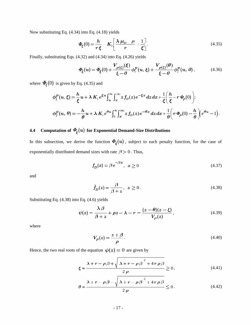
4.4 Computation of ( )u for Exponential Demand-Size Distributions
In this subsection, we derive the function ( )u , subject to each penalty function, for the case of
exponentially distributed demand sizes with rate 0 . Thus,
( )D
xf x e
, 0x (4.37)
and
( )Df zz
, 0z . (4.38)
Substituting Eq. (4.38) into Eq. (4.6) yields
( )( )( )
( )
z zz z r
z V z, (4.39)
where
( )z
V z . (4.40)
Hence, the two real roots of the equation 0( )z are given by
2
40
2
r r r , (4.41)
2
40
2
r r r . (4.42)
- 18 -
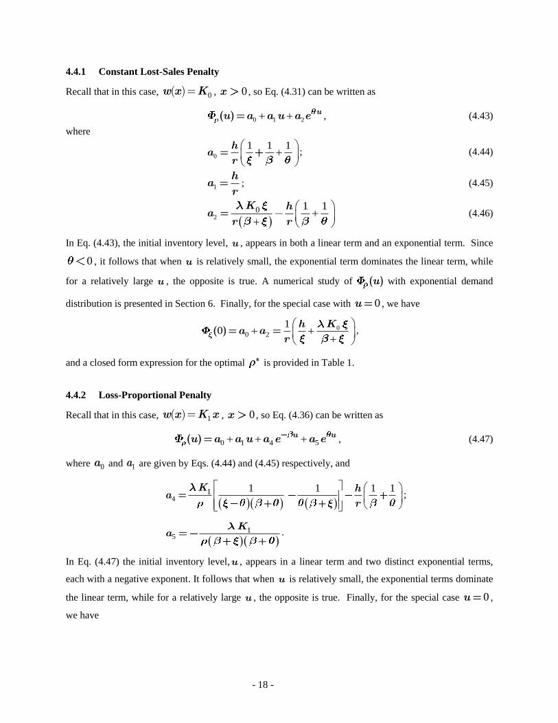
4.4.1 Constant Lost-Sales Penalty
Recall that in this case, 0w x K( )= , 0x , so Eq. (4.31) can be written as
0 1 2 ( )= uu a a u a e , (4.43)
where
0
1 1 1=
ha
r
; (4.44)
1 =h
ar
; (4.45)
20 1 1
=
K ha
r r (4.46)
In Eq. (4.43), the initial inventory level, u , appears in both a linear term and an exponential term. Since
0 , it follows that when u is relatively small, the exponential term dominates the linear term, while
for a relatively large u , the opposite is true. A numerical study of ( )u with exponential demand
distribution is presented in Section 6. Finally, for the special case with 0=u , we have
00 2
10( )= =
Kha a
r
,
and a closed form expression for the optimal * is provided in Table 1.
4.4.2 Loss-Proportional Penalty
Recall that in this case, 1w x K x( )= , 0x , so Eq. (4.36) can be written as
50 1 4 ( )= u uu a a u a e a e , (4.47)
where 0a and 1a are given by Eqs. (4.44) and (4.45) respectively, and
41 1 1 1 1
=+ +
K ha
r
;
51=
+
Ka .
In Eq. (4.47) the initial inventory level,u , appears in a linear term and two distinct exponential terms,
each with a negative exponent. It follows that when u is relatively small, the exponential terms dominate
the linear term, while for a relatively large u , the opposite is true. Finally, for the special case 0=u ,
we have

- 19 -
0 4 51 1 1
0
( )= =+
Kha a a
r,
and a closed form expression for the optimal * is provided in Table 2.
5. Optimization of the Replenishment Rate
In this section, we optimize the expected discounted cost function ( )u with respect to the
replenishment rate, , via an optimization of ( )u with respect to . We first provide a general
structural result in subsection 5.1 for an optimal replenishment rate, * (admitting the possibility of
multiple optimal replenishment rates), and then describe computational simplifications in subsection 5.2
for some selected demand-size distributions.
5.1 Optimal Replenishment Rate
Observe that the cost function ( )u , given by Eq. (4.26), is expressed in terms of the two roots, and
. In the sequel, we shall express ( )u in terms of alone by expressing in terms of . To this end,
we set 0z in Eq. (4.23), and deduce the relation as follows by the fact that 0 r( ) in light of Eq.
(4.6),
0( ) /rV . (5.1)
Substituting Eq. (5.1) into Eq. (4.26) then yields
2
2
2 0
(0) / (0) / (0) /
( )( )( )
(0)
(0) / ( ) 1
(0) (0)
( )= + ( )+
+ ( ) ++
u
u
u x
rV u rV x rV u
Vgu e g x e dx g
r rV
V rV ge g x e dx e
rV rV
(5.2)
The boundedness of ( )u guarantees the existence of a global minimizing point,
*
0
argmin= { ( )}u . However, the function ( )u is not convex in general. In fact, it is challenging
to prove the uniqueness of the global minimizer, and this still remains an open problem.
In light of Theorem 3, a minimizer, * , can be computed in several ways. A straightforward, but
relatively time-consuming method, is global search. However, when ( )u is convex, the availability of

- 20 -
the derivative ( )u
allows us to apply the relatively fast Newton’s Method. The above discussion
can be summarized as follows.
Corollary 2
Given 0( )=I u , the optimal replenishment rates for ( )u are given by
1 **
*
( )Dr f, (5.3)
where *
0
argmin= { ( )}u and ( )u is given by Eq. (5.2). □
5.2 Optimal Replenishment Rate under Delayed Replenishment
Suppose the system operates under delayed replenishment, that is, replenishment starts only after the first
lost-sale occurrence. For example, suppose the system has an initial setup period during which
replenishment is unavailable (e.g., a production facility which requires a setup time to gear up for
production). Accordingly, minimizing the corresponding expected discounted cost, ˆ ( )u , over an
infinite time horizon can be written as
0 0ˆ 0( )= ( )+ ( ) ( )u c u d u . (5.4)
From Eq. (5.4), it is readily seen that minimizing ˆ ( )u with respect to is equivalent to minimizing
0( ) with respect to , since only the second term is a function of . In the following two subsections,
we treat the optimization of 0( ) for the special cases of constant lost-sales penalty and loss-
proportional penalty.
5.2.1 Constant Lost-Sales Penalty
Recall that in this case, 0w x K( ) = , 0x , where 0 0K is a constant, and 0( ) is given by Eq.
(4.30). In view of Eq. (4.9), Eq. (4.30) can be rewritten as
0 1 ( )0
( )=Dh K f
r. (5.5)
By Eq.(5.5), the optimal * is given by
*
00 ( )
argmin D
hK f . (5.6)

- 21 -
Table 1 exhibits the optimal *, and * 0( ) with closed-form formulas, when available, for selected
demand distributions; detailed derivations are given in Appendix B.
Table 1. Optimal expected discounted costs subject to constant penalty under various demand distributions
* 0( )*
D d
0d 00
argmin
dhK e 1 *
*
dr e
* * *
*
0 h K r
r
Exp( )D
0
0
0
, if
, otherwise
hK h
K h
00
0
, if
0, otherwise
K h rK h
h K
00
0
2, if
, otherwise
K h hK h
r
K
r
( , )D U a b
0 a b 00
argmin( )
a bh e eK
b a
1
a br e e
b a
* *
* * *( )
* * *
*
0 h K r
r
( )D ,
0,
00argmin 1
hK
1 1r *
* */ * * *
*
0 h K r
r
In the table above and elsewhere, the argmin operation corresponds to a search for the optimal *,
whenever a closed form formula for it is either unavailable or not readily available. In particular, for an
exponential demand distribution, the optimal solution is available in closed form, and the condition
0K h ensures a positive optimal replenishment rate; otherwise, it is optimal to have zero
replenishment and bear the repeated penalty costs (a degenerate case).
5.2.2 Loss-Proportional Penalty
Recall that in this case, 1w x K x( ) = , for 0x , where 1 0K is constant, and 0( ) is given by
Eq. (4.35). In view of Eq. (4.9), Eq. (4.35) can be rewritten as
11
1 1 ( )0
( )= DD Kh fK
r r, (5.7)
where [ ]D D . Consequently, by Eq. (5.7), the optimal * is given by
*
10
1 ( )argmin
Dh fK . (5.8)

- 22 -
Table 2 exhibits the optimal *, and *(0) with closed-form formulas, when available, for selected
demand distributions; detailed derivations are given in Appendix B.
Table 2. Optimal expected discounted costs subject to loss-proportional penalty under various demand
distributions
* *
* 0( )
D d
0d 1
0
1argmin
dh eK
1 *
*
dr e
*
* *1 1
1 1
dh eK Kd
r
Exp( )D
0
1
1
, if
, otherwise
hK h
K h
11
1
, if
0, otherwise
K h rK h
Kh 1
1
1
2, if
, otherwise
K h hK h
r
K
r
( , )D U a b
0 a b
1
0
argmin 1( )
a bKh e e
b a
1
a br e e
b a
* *
* * *( )
* *
* *2
111
1
( ) 2
a b K b-ah K e eK
r b a
( )D ,
0,
1
0
1 1argmin
hK
1 1
r *
* */ *
* *1 1
1 11
hK K
r
Again, for an exponential demand distribution, the optimal solution is available in closed form, and the
condition 1K h ensures a positive optimal replenishment rate; otherwise, it is optimal to have zero
replenishment and bear the repeated penalty costs (a degenerate case).
6. Numerical Study
This section contains two numerical studies of production-inventory systems with selected demand-size
distributions, subject to constant lost-sales penalty. Both studies were conducted with the following
common parameters: 1= , 1h = , 0 100=K , and 0.1r = . Recall that only the exponential
demand-size distribution gives rise to a closed-form optimal solution; in all other cases, optimal solutions
were obtained by a simple search.
6.1 Optimal Numerical Solutions for Zero Initial Inventories
In this study we compute and compare the numerical values of 0( ) for increasing mean demand sizes,
and under the following demand-size distributions: constant, exponential, uniform and Gamma. Table 3

- 23 -
displays the optimal and *
as functions of the mean demand, [ ] = 1D , for the four
aforementioned demand-size distributions.
Table 3. Optimal 0( ) for selected demand-size distributions
E[ ]D 1=D / ExpD 0,2D U / 4,1 4D /
0( ) 0( ) 0( ) 0( )
0.05 0.27 44.47 0.27 44.22 0.27 44.39 0.27 44.41
0.30 0.82 108.03 0.80 106.54 0.82 107.53 0.82 107.66
1.30 2.30 221.40 2.16 215.04 2.25 219.19 2.26 219.79
3.30 4.63 346.27 4.20 330.32 4.47 340.58 4.53 342.18
5.30 6.66 432.79 5.87 407.43 6.37 423.54 6.47 426.23
6.30 7.64 468.98 6.61 439.00 7.22 457.96 7.35 461.20
7.30 8.59 501.97 7.28 467.37 8.08 489.12 8.24 492.95
8.30 9.47 532.35 7.94 493.19 8.87 517.68 9.06 522.11
9.30 10.36 560.62 8.60 516.92 9.67 544.11 9.88 549.15
10.00 10.95 579.30 9.02 532.46 10.19 561.50 10.43 566.99
15.00 14.86 693.46 11.58 624.60 13.41 666.27 13.98 675.10
20.00 18.37 784.52 13.61 694.43 16.28 747.54 16.88 760.16
25.00 21.23 860.50 15.00 750.00 18.21 813.34 19.60 830.15
30.00 23.87 925.43 16.14 795.45 19.81 867.66 21.50 889.22
From Table 3, it can be seen that the respective and the corresponding 0( ) increase in this order
of distributions: exponential, uniform, Gamma and constant. Note that as the average demand increases,
and 0( ) increase as expected. Furthermore, for each selected demand-size distribution, we observe
that [ ]D for 7[ ] D (case 1), whereas [ ]D for 15[ ] D (case 2). One
possible explanation for these observations can be derived by examining the optimal production attendant
to a demand rate, noting that discounting implies that the objective function is driven by the behavior of
the system in an initial interval (starting at 0). Thus, in case 1, the optimal production rate would be
driven above the demand rate, because otherwise, the inventory level would stay low, thereby incurring
excessive penalty costs. Conversely, in case 2, the optimal production rate would be driven below the
demand rate, because otherwise, the inventory level would stay high, thereby incurring excessive holding
costs.
The above observation can be explained analytically for the case of exponential demand, Exp( )D ,
with the aid of the explicit solution given in Table 1. In particular, assuming that 0K h holds, the

- 24 -
optimal production rate is given in closed form by 0
0
K h r
h K , whence the
difference [ ]D is given by
0
0
r K h r
h K. (6.1)
Thus, for sufficiently large , i.e., sufficiently small [ ]D , the right-hand side of Eq. (6.1) becomes
positive, implying [ ]D . Conversely, for sufficiently small but positive , i.e., sufficiently
large [ ]D , the right-hand side of Eq. (6.1) becomes negative, implying D[ ] . Furthermore,
by Eq. (6.1), the cut-off point for [ ]D is identified by
2
2 0
0
K hr r
h K. In this
numerical study with the selected parameters and 1 , it shows that the cut-off mean demand is
13.7[ ] =D . That is, [ ]D for 13.7[ ] D , whereas [ ]D for 13.7[ ] D ,
which explains our observations.
In the next numerical study, we use the same parameters as before, but fix 10[ ] =D and vary the value
of the coefficient of variation vc (ratio of standard deviation to mean) of the random demand. For each
selected value of vc , we chose the parameters of Uniform and Gamma distributions for D so as to keep
the corresponding values of vc the same. Table 4 displays several such parameter values and the
corresponding , and for selected ranging between to .
Table 4. Optimal quantities for selected demand-size distributions with respect to their coefficient of variation
vc , D U a b , D
a b * 0( ) *
0( )
1 3 0 20 0.041 10.165 561.497 3 0.300 0.041 10.242 562.971
1 2/ 1.340 18.660 0.040 10.363 566.176 4 0.400 0.040 10.404 566.983
1 3/ 4.226 15.774 0.039 10.676 573.615 9 0.900 0.039 10.691 573.768
1 4/ 5.670 14.330 0.039 10.783 576.124 16 1.600 0.039 10.785 576.171
*0( ) vc 1 3 1 4/

- 25 -
From Table 4, it can be seen that the respective and the corresponding 0( ) increase in vc . For
each case, it is shown 10[ ]=D . Note that although the variation in *, and 0( ) is not
significant compared with the change in vc , it reveals to what extent the optimal rates depend on more
than the first two moments of the demand distribution. Furthermore, observe that when the demand
distribution is , , we have larger and 0( ) than their counterparts for demand distribution
, U a b . This phenomenon can be explained by the longer tail of the , distribution [cf. De
Kok (1987)].
6.2 Optimal Numerical Solutions for Arbitrary Initial Inventory Levels
In this study we compute and compare the numerical values of *, and ( )u for selected demand-
size distributions (constant, exponential and uniform) with increasing initial inventory levels and for low
and high average demands. Table 5 and Table 6 display , * and ( )u for sample low and high
demands as functions of the initial inventory level, 0( ) =I u .
Table 5. Optimal quantities for selected demand-size distributions under a low demand with
1/ 2[ ] = =D
0( ) =I u 1=D ( )D Exp 0, 2/D U
* ( )u *
( )u * ( )u
0 0.076 3.169 272.590 0.082 2.936 262.840 0.078 3.087 269.170
5 0.130 2.530 157.450 0.113 2.515 193.450 0.113 2.614 172.160
10 0.194 2.173 150.260 0.155 2.171 181.490 0.177 2.165 163.060
15 0.301 1.835 175.720 0.208 1.893 191.810 0.215 1.996 177.840
20 0.372 1.679 197.900 0.273 1.660 212.640 0.367 1.569 204.800
25 0.513 1.445 229.660 0.357 1.447 239.160 0.387 1.528 232.330
30 0.547 1.399 262.250 0.466 1.250 269.040 0.469 1.383 264.410
35 0.717 1.202 295.100 0.610 1.065 301.060 0.674 1.119 297.570
40 1.160 0.864 330.040 0.812 0.885 334.520 1.065 0.816 329.030
45 1.714 0.623 364.120 1.109 0.712 368.970 1.439 0.644 362.650
50 7.598 0.145 392.380 1.591 0.541 404.150 3.055 0.333 396.290

- 26 -
Table 6. Optimal quantities for selected demand-size distributions under a high demand with
1/ 20[ ] = =D
0( ) =I u 1=D / ( )D Exp 0,2D U /
* ( )u *
( )u * ( )u
0 0.030 18.299 784.500 0.041 13.519 694.430 0.034 16.187 747.520
5 0.031 18.251 774.650 0.041 13.356 684.430 0.034 16.187 736.510
10 0.032 17.943 759.150 0.043 13.147 676.910 0.034 16.187 726.210
15 0.032 17.943 736.390 0.044 12.928 671.680 0.037 15.709 716.850
20 0.032 17.943 705.290 0.045 12.685 668.580 0.037 15.709 709.080
25 0.035 17.324 705.480 0.047 12.437 667.440 0.039 15.203 703.600
30 0.036 16.994 707.410 0.049 12.171 668.130 0.039 15.203 700.800
35 0.036 16.994 705.130 0.051 11.889 670.500 0.042 14.642 698.260
40 0.040 16.303 706.100 0.053 11.609 674.430 0.042 14.642 698.590
45 0.040 16.303 709.320 0.055 11.317 679.790 0.045 14.073 701.890
50 0.042 15.929 715.630 0.058 11.007 686.490 0.045 14.073 707.640
Table 5 and Table 6 above reveal similar behavior patterns of and ( )u , as functions of 0( ) =I u .
For each demand-size distribution in each table, decreases as 0( ) =I u increases, while the
corresponding ( )u first decreases and then increases in u . Also, for any given initial inventory level,
( )u increases as the average demand, [ ]D , increases. Moreover, for each demand-size
distribution, the optimal initial inventory level 0
argmin ( )u
u u{ } increases in the average demand.
For example, 10=u in Table 5 and 25 35[ , ]u in Table 6 are cases in point. In other words, a larger
demand size is more beneficial when the initial inventory level is high. This is intuitive since higher
demand is more likely to deplete the inventory quickly, which reduces the holding cost incurred due to a
high initial inventory level. We also observe that in each of these tables, decreases in the demand-size
distribution in this order: constant, uniform and exponential; this, however, does not generally hold for
( )u .
7. Time-Average Cost and Optimization
The long-run time-average (undiscounted) cost can be treated similarly to its discounted counterpart. In
this case, we need to assume the stability condition, [ ]D (or equivalently 1[ ]< );

- 27 -
otherwise the long-run time-average cost is infinite. In the sequel, we derive the time-average cost
directly from the results for the discounted cost by taking limits as 0r and using the renewal reward
theorem (cf. Ross (1996)).
For 0r , the Lundberg’s fundamental equation of Eq. (4.7) becomes
0( )Df z z . (7.1)
Under the stability condition [ ]D , it follows that Eq. (7.1) has two real roots: 0 0 and
0 0 . Next, by Eqs. (3.1) and (7.1), one has
0( )DF , (7.2)
which implies that and 0 are connected by a bijection.
In view of Eq. (7.2), the stability condition [ ]D can be written as 0( ) [ ]DF D . Since
( )DF z is monotonically decreasing in z and ( ) [ ]DF z D at 0z , the stability condition
[ ]D in the PRR space, can be equivalently expressed as 0 0 in the LPR space.
Under the stability condition 0 0 in the LPR space (i.e., [ ]D in the PRR space), the
inventory process over time intervals of the form 1, i i is a renewal process, and the corresponding
cost process can be regarded as a renewal reward process, with finite expectations of inter-renewal times
and cycle rewards. Consequently, by Theorem 3.6.1 in Ross (1996), the long-run time-average cost is
independent of the initial inventory level, and can be represented by
1
0
0 0
( )=
[ | ( )= ]
cc
I, (7.3)
where 0( )c is given by Eq. (3.6) with 0r and 0u . Next, we use 0 as the decision variable to
derive c in closed form and analyze its optimal solution. Following our notational fashion, we let c
and 0
c denote the time-average cost function of Eq. (7.3) in terms of and 0 , respectively. To
derive the time average cost, we use the fact that ( )d u , defined by Eq. (4.2), can be interpreted as the
moment generating function of 1 at r ; cf. Karr (1993). Consequently, by Eq. (4.16), the expected
time to the first shortage conditioned on the initial inventory level can be written as
1
0 0
1 10 0
( )[ | ( )= ] =
D
If
. (7.4)

- 28 -
Note also that Eq. (7.4) can be interpreted as the expected value of the time to ruin in the classical
insurance model [cf. Gerber and Shiu (1998)], conditioned on a zero initial surplus level. The following
theorem provides a closed form expression for the time-average cost.
Theorem 4
Under the stability condition [ ]D , the time-average cost is given by
00 0( )=c g , (7.5)
where 0 0 . □
We mention that De Kok (1987) studies a corresponding production-inventory system, but with two
switchable production rates, and provides an approximation for the time-average of inventory holding and
switching cost (cf. Eq. (2.10) therein). Actually, our production-inventory model can be treated as the
aforementioned model, provided the two production rates as the equal and there is no switching cost. In
this case, the approximated carrying cost in De Kok (1987) is exactly equivalent to the time-average
holding cost in Eq. (7.5). However, the approximation proposed by De Kok (1987) only accounts for the
holding cost but ignores the lost-sale penalty component.
In view of Theorem 4, minimizing c with respect to is equivalent to minimizing 0
c with respect to
the positive variable 0 . To this end, we first optimize 0 0 0( )=c g in the LPR space to find the
optimal *
0 , and then compute the corresponding optimal * in the PRR space. The following corollary
provides a general structural result for the optimal replenishment rate, * .
Corollary 3
The optimal replenishment rate for the time-average cost c under the stability condition [ ]D is
given by
0 * *( )DF , (7.6)
where *
0
0 0 00
argmin ( )= { }g . (7.7)
□
- 29 -
8. Further Extensions
The research presented in this paper can be extended in several directions. First, the methodology can be
extended to include in the objective function a variable production cost modeled as a nonnegative and
increasing function of the replenishment rate. In this case, the expected discounted production cost
is
0
rt av a e dt
r= = . (8.1)
By Eq. (4.9), we can rewrite v in Eq. (8.1) as
( )
D
ra F
vr
= , (8.2)
where v and v denote the same cost function, but of and , respectively. Finally, we can express
the total expected discounted cost function as ( )+u v , where ( )u is given by Eq. (5.2) and v
by Eq. (8.2). This closed form of the objective function allows one to compute the optimal * directly,
from which the optimal replenishment rate * can be recovered via Eq. (5.3).
For the case of time-average cost, adding the production cost to Eq. (7.5) yields the total cost
function representation
0 0 0 0 0( ) ( ) ( ) Da g a F g , (8.3)
by virtue of Eq. (7.2). The above closed form expression allows one to compute the optimal *0 directly.
The requisite optimal replenishment rate * can then be obtained from Eq. (7.6).
Second, we point out that the results of this paper can be applied to cost optimization (discounted or time-
average) subject to a given service-level constraint, e.g., a fill rate , defined as the percentage of
demand arrivals that are immediately satisfied in full from inventory on hand. Let the lost-sales rate be
denoted by 1= . Then, lim
= ( )/ ( )t B AN t N t , where ( )AN t and ( )BN t denote the number
of demand arrivals and lost-sale occurrences, respectively, in the interval 0( ],t . The lost-sales rate, ,
can be alternatively represented as [cf. Ross (1996), Theorem 3.4.4]

- 30 -
1
1 0 0
[ ]=
[ | ( )= ]
T
I. (8.4)
Substituting 1 1[ ]= /T and Eq. (7.4) into Eq. (8.4) yields
001 ( )= = Df . (8.5)
Consequently, we have the following representation for the fill rate
0( )= Df . (8.6)
For optimization problems with objective functions of expected discounted cost or long-run time-average
cost, constrained by a given minimal fill rate, 0 1' , one can apply Eq. (8.6) to compute the
critical value ' such that ( ) =Df ' ' . It follows that the cost optimization problem (e.g., the time
average cost studied in Section 7) with a constrained fill rate, ' , can be solved by a search in the LPR
space, restricted to the interval 00 ' , in lieu of the original search space, 0 0 .
9. Conclusions and Future Research
This paper investigated a continuous-review single-product production-inventory system with a constant
replenishment rate, compound Poisson demands and lost-sales. Two objective functions that represent
metrics of operational costs were investigated: (1) the sum of the expected discounted inventory holding
costs and the lost-sales penalties, over an infinite time horizon, given an initial inventory level; and (2) the
long-run time-average of the same costs. A bijection between the PRR space and LPR space was
established to facilitate optimization. For any initial inventory level, a closed form expression was
derived for the expected discounted cost, given an initial inventory level, in terms of an LPR variable. The
resultant cost function was then readily optimized in the LPR space, and the requisite optimal value of the
replenishment rate was recovered via the aforementioned bijection. In addition, the time-average cost
was also derived in closed form under a stability condition, and an optimization methodology similar to
the one used for the expected discounted cost, was applied to optimize the requisite time-average cost.
Additional work in this area may include the following. First, for the general model (with general cost
functions and general demand distributions), one might admit multiple optimal replenishment rates,
though it is likely that a single optimal replenishment rate is unique under fairly general conditions. The
type of conditions necessary to ensure uniqueness is a future research topic. Second, one might introduce
inventory capacity constraints (e.g., base stock level), such that replenishment is suspended or shut down
when the inventory level reaches or is at capacity. Third, it is of interest to investigate similar production-
inventory systems with discrete replenishment, that is, where replenishment orders are triggered by

- 31 -
demand arrivals that drop the inventory level below some prescribed base stock level. Finally, regarding
the discrete-time version of these problems, we note that the integro-differential equation obtained in
Lemma 1 is no longer valid, since its derivation is based on time continuity. Therefore, a different
approach which utilizes Markov chain and/or renewal theory might be employed to treat the
corresponding discrete-time models.
Acknowledgments
We are indebted to the Area Editor, the Associate Editor and three anonymous referees for many
constructive comments and useful suggestions.
References
[1] Adan, I., O. Boxma, and D. Perry (2005) “The G/M/1 queue revisited”, Mathematical Methods of
Operations Research, 62(3), 437-452.
[2] Asmussen, S. (2000) Ruin Probabilities, Advanced Series on Statistical Science & Applied
Probability, World Scientific.
[3] Asmussen, S. (2003), Applied Probability and Queues, Springer, 2nd Edition.
[4] Bell, C.E. (1971) “Characterization and computation of optimal policies for operating an M/G/1
queuing system with removable server”, Operations Research, 19(1), 208-218.
[5] Boxma, O.J., A. Löpker and D. Perry (2011) “Threshold strategies for risk processes and their
relation to queueing theory”, Journal of Applied Probability, 48A (Special volume), 29-38.
[6] Churchill, R. V. (1971) Operational Mathematics, McGraw-Hill Book Company.
[7] Cohen A. M. (2007) Numerical Methods for Laplace Transform Inversion, Springer.
[8] De Kok, A.G., (1985) “Approximations for a lost-sales production/inventory control model with
service level constraints”, Management Science, 31,729–73.
[9] De Kok, A.G. (1987), “Approximations for operating characteristics in a production-inventory
model with variable production rate”, European Journal of Operational Research, Vol. 29 (3), 286-
297.
[10] De Kok, A.G., H.C. Tijms, and F.A. Van Der Duyn Schouten (1984) “Approximations for the single
product production-inventory problem with compound Poisson demand and service level
constraints”, Advances in Applied Probability. 16, 378-401.
[11] Doshi, B.T., F.A. Van der Duyn Schouten, and A.J.J. Talman (1978) “A production inventory
control model with a mixture of back-orders and lost-sales”, Management Science, 24, 1078–1086.
[12] Gavish, B. and S.C. Graves, (1980) “A One-product production/inventory problem under continuous
review policy”, Operations Research, 28(5), 1228-1236.
[13] Gerber H.U. and S.W. Shiu (1997) “The joint distribution of the time of ruin, the surplus
immediately before ruin and the deficit at Ruin”, Insurance: Mathematics and Economics. 21, 129-
137.
[14] Gerber, H.U. and E.S.W. Shiu (1998) “On the time value of ruin”, North American Actuarial
Journal, 2, 48-78.
[15] Graves, S.C. and J. Keilson (1981) “The compensation method applied to a one-product production
inventory model”, Mathematics of Operations Research, 6, 246-262.

- 32 -
[16] Graves, S. C. (1982) “The application of queueing theory to continuous perishable inventory
systems”, Management Science, 28, 400-406.
[17] Grunow, M., H. O. Günther, and R. Westinner (2007) “Supply optimization for the production of
raw sugar”, International Journal of Production Economics, 110, 224- 239.
[18] Heyman, D. P. (1968) “Optimal operating policies for M/G/1 queuing systems”, Operations
Research, 16(2), 362-382.
[19] Jacobs, F. R. and R. B. Chase (2013). Operations and supply management. New York, NY:
McGraw-Hill, 14th Edition.
[20] Lee, H and M. M. Srinivasan (1989) “Control policies for the Mx/G/1 queueing system”,
Management Science, 35(6), 708-721.
[21] Lin, X.S. and K.P. Pavlova (2006) “The compound Poisson risk model with a threshold dividend
strategy”, Insurance: Mathematics and Economics, 38(1), 57-80.
[22] Lin, X.S., G.E. Willmot and S. Drekic (2003) “The classical risk model with a constant dividend
barrier: analysis of the Gerber-Shiu discounted penalty function”, Insurance: Mathematics and
Economics. 33, 551-566.
[23] Löpker, A. and D. Perry (2010) “The idle period of the finite G/M/1 queue with an interpretation in
risk theory”, Queueing Systems, 64, 395-407.
[24] Lundberg, F. (1932), “Some supplementary researches on collective Risk theory”, Skandinavisk
Aktuarietidskrift 15: 137-58.
[25] Mandatory Reporting of Greenhouse Gases - Part 3 of 9, Federal Register, 10 April 2009, 74(068).
[26] Perry, D. 2011. The G/M/1 Queue. Wiley Encyclopedia of Operations Research and Management
Science.
[27] Perry, D., W. Stadje and S. Zacks (2005) “Sporadic and continuous clearing policies for a
production/inventory system under an M/G demand process”, Mathematics of Operations Research,
30(2), 354-368.
[28] PixTech Hits Production Milestone, Display Development News, Nov. 1st, 2000.
[29] Prabhu, N.U. (1965) Queues and Inventories: A study of their basic stochastic processes, John Wiley
& Sons, Inc.
[30] Prabhu, N.U. (1997) Stochastic Storage Processes: Queues, Insurance Risk, Dams and Data
Communication. 2nd Ed, Springer.
[31] Ross, S.M. (1996) Stochastic Processes, Wiley Series in Probability and Mathematical Statistics,
2nd Edition.
[32] Saff, E. B. and A. D. Snider (1993) Fundamentals of Complex Analysis for Mathematics, Science,
and Engineering, Prentice Hall.
[33] Scarf, H. (1960) “The optimality of (s, S) policies for the dynamic inventory problem”, Proceeding
of the 1st Stanford Symposium on Mathematical Methods in the Social Sciences, Stanford University
Press, Stanford, CA.
[34] Shortle, J. F., P.H. Brill, M. J. Fischer, D. Gross and D. M.B. Masi (2004) “An algorithm to compute
the waiting time distribution for the M/G/1 queue”, INFORMS Journal on Computing, 16, 2.
[35] Sobel, M. J. (1969) “Optimal average-cost policy for a queue with start-up and shut-down costs”,
Operations Research, 17(1), 145-162.
[36] Widder, D. V. (1959) The Laplace transform, Princeton University Press.
[37] Biotech/Biomedical: Cell-Free Protein Production. Membrane & Separation Technology News. 1
April 1997.

- 33 -
Appendix A
A.1 Proof of Lemma 1
For any given initial inventory level 0u , consider a time interval 0( , ]s , 0s . We have the
following two disjoint events and the corresponding conditional expected discounted cost functions on
those events:
(1) On the event 1{ }A s , the corresponding conditional expected discounted cost is
11
0
0
1 0{ }[ ( ) | ( ) =
( ) ( )
( ) ( ) .
A s
t rz rs
s rz rs
s
s
s
C I u
e h u z e dz c u s e dt
e h u z e dz c u s e
]
= (A.1)
Here, the first term in the integral above is the discounted holding cost over 0( , ]s , the second is the
discounted residual cost over 1( ]s , and we use the relation 1 1{ } { }A s s .
(2) On the event 1{ }A s , the corresponding conditional expected discounted cost can be expressed
as
110
1 0{ }( ) | ( ) = ,s t
A sC I u e M u t dt( ) , (A.2)
where 1 1 0, ( )| , ( ) =M u t C A t I u( ) = is given by
0 0
, ( ) ( ) ( )
+ ( ) ( )
D
D
t u tr z r t
r t
u t
M u t h u z e dz e f x c u t x dx
e f x w x u t dx
( )
( ) (A.3)
Next, adding Eqs. (A.1) and (A.2) yields
0 0 0
0 0
0
( ) ( )
( )
( ) ( ) ( )
( ) ( ) ( )
+ ( ) ( )
D
D
r zs s tr z ts
s u tr s r t
s r t
u t
c u he u z e dz h e u z e dzdt
c u s e e f x c u t x dxdt
e f x w x u t dxdt( )
(A.4)

- 34 -
In the following, we shall prove the continuity and differentiability of ( )c u for 0u . To prove
continuity, let 0s in Eq. (A.4), and observe that 0
lim( ) ( + )s
c u c u s since all the integrals on
the right hand side vanish.
We proceed to prove differentiability by definition. By Eq. (A.4), one has
0 0 0
0 0
0
1
1 1 1
1
( ) ( )
( )
( ) ( )
( ) ( )
( ) ( ) ( )
( )
D
D
r zs s ts r z t
s u tr s r t
s r t
u t
c u s c u
s
h e u z e dz h e u z e dzdts
c u s e e f x c u t x dx dts s
e f x w xs
( ( )u t dxdt)
The equation above shows that ( )c u is right differentiable by taking the limit 0s (equivalently, as
0s ) and the right derivative is
0
( ) ( ) ( ) ( )
( )
D
D
u
u
h u rc u c u f x c u x dxdt
u
f x w x u dxdt( )
(A.5)
For 0 /s u , replacing u with u s in Eq. (A.4) yields
0 0 0
0 0
0
( ) ( )
( )
( ) ( ) ( )
( ) ( ) ( )
+ ( ) ( )
D
D
r zs s tr z ts
s u s tr s r t
s r t
u s t
c u s he u s z e dz h e u s z e dzdt
c u e e f x c u s t x dxdt
e f x w x u s t( )dxdt
From the equation above, one further has

- 35 -
0 0 0
0 0
0
1 1 1
1
( ) ( )
( )
( ) ( )
( ) ( )
( ) ( ) ( )D
r zs s ts r z t
s u s tr s r t
s r t
c u s c u
s
h he u s z e dz e u s z e dzdt
s s
c u e e f x c u s t x dxdts s
es
( ) ( ) .Du s t
f x w x u s t dxdt( )
In a similar vein, the equation above implies that ( )c u is left differentiable by taking the limit 0s
(equivalently, as 0s ), which yields the same expression as that of Eq. (A.5). Thus, ( )c u is
differentiable for 0u (its derivative at 0=u is given by the right derivative).
Finally, we conclude that Eq. (A.5) holds for both the left and right derivatives for 0u , and the
remainder of the proof of Eq. (4.4) uses Eq. (4.5) and simple rearrangement of terms. □
A.2 Proof of Lemma 2
To prove part (a), note that by Eq. (4.8),
1 ( )Dr
f . (A.6)
Eq. (4.9) now follows from the above equation with the aid of Eq. (3.1). Furthermore, Eq. (4.9) defines
implicitly a mapping from the PRR space to the LPR space. This mapping is one-one, since by
Eq. (4.9), 1 2( )= ( ) implies 1 2 ; it is onto, since every 0 inverse maps to some 0 ,
again by Eq. (4.9). This mapping is, therefore, a bijection.
To prove part (b), we differentiate Eq. (4.9) with respect to , yielding
2 01
( )( ) ( )
( )
xD
rxe F x dx .
The equation above implies that 0( ) since each term in the brackets on the right-hand side above
is strictly positive for all 0 , which in turn implies the requisite result.
- 36 -
Next, we prove 0
lim
( ) in part (1) of (b) by contradiction. Suppose 0
lim
( ) exists.
Then, the following positive limit exists,
0 0lim 0
D Dr r
L F F+ ( ( )) + ( )>( )
.
However, taking the limit on both sides of Eq. (4.9) as 0 yields 0 0L , which contradicts the
above, thereby establishing the requisite result.
To prove 0
lim
( ) +r in part (1) of (b), note that Eq. (4.8) can be rewritten as
Dr f( ) + ( ( )) . (A.7)
Since 0
lim
( ) (just proven before) implies 0
lim ( ) 0 Df ( ) , the requisite result now follows
by taking the limits as 0 on both sides of Eq. (A.7).
Next, we prove lim 0
( ) in part (2) of (b) by contradiction. Suppose lim 0
( ) exists.
Then, the following finite limit exists,
lim
D Dr r
L F F+ ( ( )) + ( )<( )
.
However, sending on both sides of Eq. (4.9) yields L , which contradicts the above,
thereby establishing the requisite result.
Finally, to prove lim
( ) r in part (2) of (b) we again use Eq. (A.7). Since lim 0
( ) (just
proven before) implies lim ( ) 1
Df ( ) , the requisite result now follows by taking the limits as 0
on both sides of Eq. (A.7). □

- 37 -
A.3 Proof of Proposition 1
For 0 , Eq. (4.12) follows by setting z in Eq. (4.11) and noting that its first term now vanishes
by virtue of the equation 0( ) . Eq. (4.13) follows immediately by substituting Eq. (4.12) into Eq.
(4.11) and dividing the resultant equation by 0( )z . □
A.4 Proof of Proposition 2
To prove Eq. (4.16), consider the special case where 0h and 1w x( ) = for 0x . In this case, Eq.
(3.6) implies
( )= ( )c u d u , (A.8)
and Eq. (4.5) becomes
( ) ( ) ( )D Du
g u f x dx F u , (A.9)
while in view of Eqs. (A.8) and (A.9), Eq. (4.12) becomes
0( ) ( )Dd F . (A.10)
By virtue of Eqs. (3.1) and (4.6), we further have
( )( )D
z r zF z
z. (A.11)
Consequently, setting z above, noting that 0( ) , and substituting the resultant DF ( ) into Eq.
(A.10) yields Eq. (4.16).
To prove Eq. (4.17), we take the Laplace transform of Eq. (A.9) and substitute it into Eq.(4.13) to obtain
( ) ( ) ( )( )
D Dd z F F zz
, z . (A.12)
Finally, Eq. (4.17) follows by substituting Eq. (A.11) into Eq. (A.12). □
A.5 Proof of Theorem 2
Setting 0=u in Eq. (4.1) and rearranging yield

- 38 -
00
1 0
( )( )
( )
( )( )=
( )
c
d. (A.13)
Eq. (4.18) now follows by substituting Eqs. (4.12) and (4.16) into Eq. (A.13). Finally, Eq. (4.19) follows
readily by substituting Eq. (4.18) into Eq. (4.1), while Eq. (4.20) obtains by taking Laplace transforms of
both sides of Eq. (4.19) and substituting ( )c z from Eq. (4.13) and ( )d z from Eq. (4.17). □
A.6 Proof of Corollary 1
Eq. (4.20) can be rewritten as
( ) 1 1 ( )( )
( )
g gz g z
r z z z( )= .
Eq. (4.21) now follows by inverting the equation above, noting that ( )
0g
r= ( ) by Eq. (4.18) and
( )( ) ( )
gg z G z
z= by Eq. (4.22). □
A.7 Proof of Theorem 3
To prove Theorem 3, we first show that the inverse Laplace transform of 1
z( ) is given by
1 1 ( ) ( )( ) ( )
( )
u uV Vu u e e
zL , (A.14)
where the values of ( )V and ( )V are the limits of ( )V z at and , given by Eq. (4.24) and Eq.
(4.25), respectively. This inverse Laplace transform is obtained by a standard application of the Residue
Theorem [Churchill (1971)] and contour integration, and by taking advantage of the fact that Lundberg’s
fundamental equation 0( )z has two distinct roots, and . Accordingly, by Eq. (4.23),
1
( )
( ) ( )( )
V z
z z z, (A.15)
where and are singularities of 1
( )z. Taking the inverse Laplace transform of Eq. (A.15) yields

- 39 -
1 1 1
2
( )lim
( ) ( )( )
iR zx
R iR
V zx e dz
z i z z( ) =L
for any real . To see that, define for R a counter-clock contour path
R R RC H L (see Figure 4), where
2 2 2= ( , ) : ( ) ,RH x iy x y R R x
( ) : ,RL x,iy x R y R .
Figure 4. Contour integral for the inverse Laplace transform
Hence, the contour integral can be written as
1 1 1 1 1 1
2 2 2( ) ( ) ( )R R
iRzx zx zx
C H iRe dz e dz e dz
i z i z i z, (A.16)
and by the Residue Theorem and Eq. (A.15), the left-hand side of Eq. (A.16) becomes
1 1
2
( ) ( )
( )R
zx u u
C
V Ve dz e e
i z. (A.17)
Eq. (A.14) now follows by substituting Eq. (A.17) into Eq. (A.16) and sending R , since the first
term on the right-hand side of Eq. (A.16) vanishes in view of the fact that for any 0x , and we have
[cf. Saff and Snider (1993)],
10lim lim
( ) ( )R RR
zx
RxH
Re dz
z R e.
- 40 -
Next, in view of Eq. (A.14), the convolution term in Eq. (4.21) becomes
0 0
( ) ( )( ) ( )e
( ) ( )( )=u uu x u x
V VG u e G x e dx G x e dx , (A.18)
where ( )G x is given by Eq. (4.22). Now, substituting Eqs. (4.18) and (A.18) into Eq. (4.21) yields
0 0
( ) ( )( )( ) ( )e
( ) ( )( )= +u uu x u x
V Vgu e G x e dx G x e dx
r, (A.19)
Finally, Eq. (4.26) follows by substituting Eq. (4.22) into Eq. (A.19) and simplifying. □
A.8 Proof of Theorem 4.
For 0r , Eq. (4.12) becomes
0
10 ( )( )c g .
Eq. (7.5) readily follows by substituting 0
10 ( )( )c g and 1
0
10 0[ | ( )= ]=I (cf. Eq. (7.4) )
into Eq. (7.3) and simplifying. □

- 41 -
Appendix B
B.1 Proofs of Table 1 Formulas
Constant Demand Size. Consider the first distribution row of Table 1, where 0D d is a constant,
so that
Df z zd( ) exp{ } . (B.1)
The corresponding * follows by substituting Eq. (B.1) into Eq. (5.6); the corresponding follows by
substituting this * and Eq. (B.1) into Eq. (5.3); and the corresponding 0( ) follows by substituting
these and into Eq. (5.5).
Exponentially-Distributed Demand Size. Consider the second distribution row of Table 1, where
Exp( )D . Substituting Eq. (4.38) into Eq. (5.6) yields
* 0
0
argmin
Kh. (B.2)
Finally, the corresponding * is obtained from Eq. (B.2) by taking the first derivative with respect to ;
the corresponding follows by substituting this *
into Eq. (5.3); and the corresponding 0( )
follows by substituting this into Eq.(5.5).
Uniformly-Distributed Demand Size. Consider the third distribution row of Table 1, where
( , )D U a b , so that
( )( )D
az bze e
f zb a z
. (B.3)
The corresponding * follows by substituting Eq. (B.3) into Eq. (5.6); the corresponding follows by
substituting this * and Eq. (B.3) into Eq. (5.3); and the corresponding 0( ) follows by substituting
these and into Eq. (5.5).
Gamma-Distributed Demand Size. Consider the fourth distribution row of Table 1, where
( )D , , so that
*
*
*

- 42 -
1( )D
zf z . (B.4)
The corresponding * follows by substituting Eq. (B.4) into Eq. (5.6); the corresponding follows by
substituting this * and Eq. (B.4) into Eq. (5.3); and the corresponding 0( ) follows by substituting
these and into Eq. (5.5). □
B.2 Proofs for Table 2 Formulas
Constant Demand Size. Consider the first distribution row of Table 2, where =D d . The
corresponding *
follows by substituting Eq. (B.1) into Eq. (5.8); the corresponding follows by
substituting this * and Eq. (B.1) into Eq. (5.3); and the corresponding 0( ) follows by substituting
these and into Eq. (4.35).
Exponentially-Distributed Demand Size. Consider the second distribution row of Table 2, where
Exp( )D . Substituting Eq. (4.38) into Eq. (5.8) yields
* 1
0
argmin
Kh. (B.5)
The corresponding * is obtained from Eq. (B.5) by taking the first derivative with respect to ; the
corresponding follows by substituting this * into Eq. (5.3); and the corresponding 0( ) follows
by substituting this into Eq. (4.35).
Uniformly-Distributed Demand Size. Consider the third distribution row of Table 2, where
( , )D U a b . The corresponding * follows by substituting Eq. (B.3) into Eq. (5.8); the corresponding
follows by substituting this * and Eq. (B.3) into Eq. (5.3); and the corresponding 0( ) follows by
substituting these and into Eq.(4.35).
Gamma-Distributed Demand Size. Consider the fourth distribution row of Table 2, where
( )D , . The corresponding * follows by substituting Eq. (B.4) into Eq. (5.8); the corresponding
follows by substituting this * and Eq. (B.4) into Eq. (5.3); and the corresponding 0( ) follows by
substituting these and into Eq. (4.35). □
*
*
*
*
*