UCRL-ID-119706

Production and Preliminary Testing of Multianalyte Imaging Sensor Arrays

James B. Richards, Steve B. Brown, and Fred P. Milanovich Measurement Sciences Group

Environmental Programs Directorate Lawrence Livermore National Laboratory

Livermore, CA 94550, USA

Brian G. Healey, Suneet Chadha, and David R. Walt Max Tishler Laboratory for Organic Chemistry

Tufts University Medford, MS 02155, USA

November 19 94

This is an informal report intended primarily for internal or limited external distribution. The opinions and conclusions stated are those of the author and may or may not be those of the Laboratory. Work performed under the auspices of the US. Department of Energy by the Lawrence Livermore National Laboratory under Contract W-74.05-Eng-48.

7 /h ~ T R l S U Y I O N OF THIS DOCUMENT I$ UVm31TFfiJ

DISCLAIMER

-

This document was prepared as an account of work sponsored by an agenq of the United States Government. Neither the United States Government nor the University of California nor any of their employees, makes any warranty, express or implied, or assumes any legal liability or responsibility for the accuracy, completeness, or usefulness of any information, apparatus, product, or process disclosed, or represents that its use would not infringe privately owned rights. Reference herein to any speafic commercial product, p!ocess, or service by trade name, trademark, manufacturer, or otherwise, does not necessarily constitute or imply its endorsement, recommendation, or favoring by the United States Government or the University of California. The views and opinions of authors expressed herein do not necessarily state or reflect those of the United States Government or the University of California, and shall not be used for advertising or product endorsement purposes.

This report has been reproduced directly from the best available copy.

Available to DOE and DOE contractors from the Office of Scientific and Technical Information

P.O. Box 62, Oak Ridge, TN 37831 Prices available from (615) 576-6401, FTS 626-8401

Y

Available to the public from the National Technical Information Service

U.S. Department of Commerce 5285 Port Royal Rd.,

Sprin$eld, VA 22161

DISCLAIMER

Portions of this document may be illegible in electronic image products. Images are produced from the best available original document.

I

Production and Preliminary Testing of Multianalyte Imaging Sensor Arrays

James B. Richards, Steve B. Brown, and Fred P. Milanovich Measurement Sciences Group

Environmental Programs Directorate Lawrence Livermore National Laboratory

Livermore, C A 94550, USA

Brian G. Healey, Suneet Chadha, and David R. Walt Max Tishler Laboratory for Organic Chemistry

Tufts University Medford, MA 02155, USA

This report covers the production and preliminary testing of fiber optic sensors that contain a discrete array of analyte specific sensors on their distal ends. The development of the chemistries associated with this technology is covered elsewhere.lt2

Part 1 - Production of multianalyte fiber optic sensors

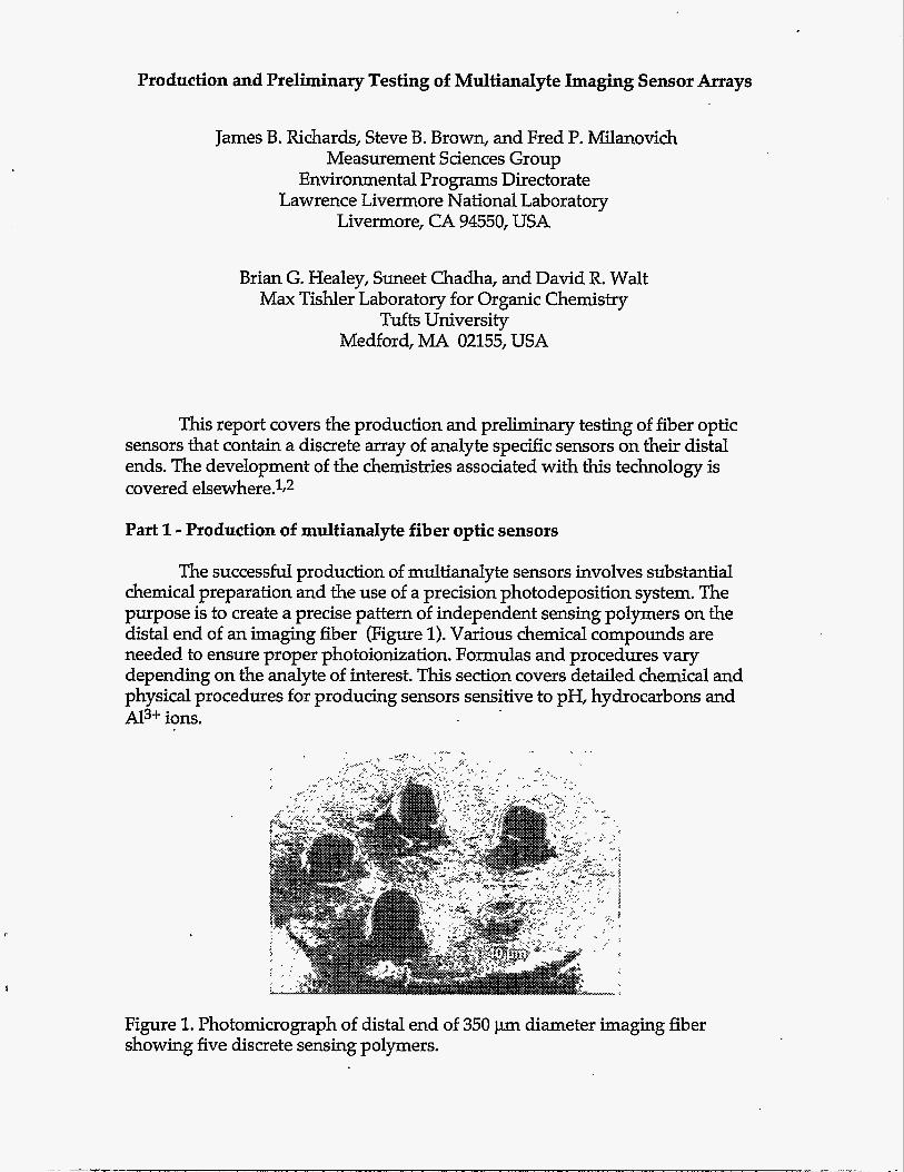
The successful production of multianalyte sensors involves substantial chemical preparation and the use of a precision photodeposition system. The purpose is to create a precise pattern of independent sensing polymers on the distal end of an imaging fiber (Figure 1). Various chemical compounds are needed to ensure proper photoionization. Formulas and procedures vary depending on the analyte of interest. This section covers detailed chemical and physical procedures for producing sensors sensitive to pH, hydrocarbons and A I S + ions.

Figure 1. Photomicrograph of distal end of 350 pm diameter imaging fiber showing five discrete sensing polymers.

Materials

Ethylene glycol dimethacrylate and 2-hydroxyethyl methacrylate were purchased from Polysciences. Inc. (80-85%) dimethyl (15-20%) (acryloxypropyl) methylsiloxane copolymer and (97-98%)dimethyl(2-3%) (methacryloxypropyl) methylsiloxane copolymer were purchased from United Chemical Technologies. Lumogallion and 5-amino eosin were purchased from Pflatz & Bauer and Molecular Probes, respectively. Nile Red and N-(3-Aminopropyl)- methacrylamide hydrochloride were purchased from Kodak. Remaining reagents were purchased from Aldrich Chemical Co. All reagents were used without further purification.

were comprised of 3000 individual elements with diameter of approximately 6 pm and numerical aperture of 0.35. Two foot lengths of fiber were polished using a polishing bushing and a polishing kit from Fiberoptics, Inc. The distal end of the fiber was cleaned with concentrated H2SO4.

Imaging fibers, purchased from Sumitomo, had a 350 pm diameter and

Deposition system

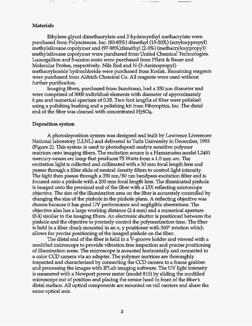
A photodeposition system was designed and built by Lawrence Livermore National laboratory (LLNL) and delivered to Tufts University in December, 1993 (Figure 2). This system is used to photodeposit analyte sensitive polymer matrices onto imaging fibers. The excitation source is a.Hamamatsu model L2481 mercury-xenon arc lamp that produces 75 Watts from a 1.0 nun arc. The excitation light is collected and collimated with a 50 mm focal length lens and passes through a filter slide of neutral density filters to control light intensity. The light then passes through a 350 nm/80 nm bandpass excitation filter and is focused onto a pinhole with a 200 mm focal length lens. The illuminated pinhole is imaged onto the proximal end of the fiber with a 15X reflecting microscope objective. The size of the illumination area on the fiber is accurately controlled by changing the size of the pinhole in the pinhole plane. A reflecting objective was chosen because it has good U V perfonnance and negligible aberrations. The objective also has a large working distance (2.4 mm) and a numerical aperture (0.4) similar to the imaging fibers. An electronic shutter is positioned between the pinhole and the objective to precisely control the polymerization time. The fiber is held in a fiber chuck mounted in an x, y positioner with 360" rotation which allows for precise positioning of the imaged pinhole on the fiber.

The distal end of the fiber is held in a V-groove holder and viewed with a modified microscope to provide vibration free inspection and precise positioning of illumination areas. The microscope is mounted horizontally and connected to a color CCD camera via an adapter. The polymer matrices are thoroughly inspected and characterized by connecting the CCD camera to a frame grabber. and processing the images with IPLab imaging software. The U V light intensity is measured with a Newport power meter (model 815) by sliding the modified microscope out of position and placing the sensor head in front of the fiber's distal surface. All optical components are mounted on rail carriers and share the same optical axis.

2

,

XY-Positioner V-groove Modified

Rotation and Holder Fiber Chuck

with 360 O Fiber Microscope Sony Color

CCD Camera

I

Hg-xe Neutral ~ - f o c ~ s ~ g Electronic Lamp Density Lens Shutter

I I I I I I

Gdhnating Excitation Pinholes 15X Reflecting Lens Filters Microscope

Objective

has ing Fiber

Microscope- CCD Camera

Adapter

Figure 2. Schematic of photodeposition system.

Imaging system

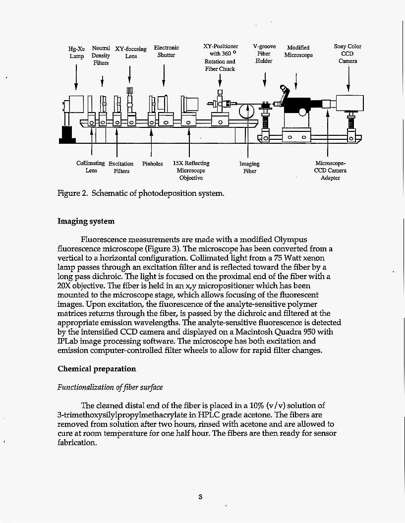
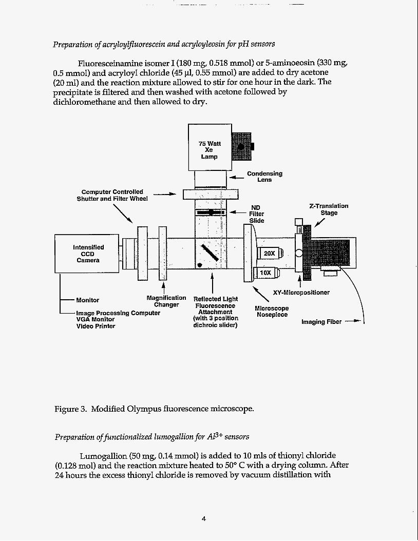
Fluorescence measurements are made with a modified Olympus fluorescence microscope (Figure 3). The microscope has been converted from a vertical to a horizontal configuration. Collimated light from a 75 Watt xenon lamp passes through an excitation filter and is reflected toward the fiber by a long pass dichroic. The light is focused on the proximal end of the fiber with a 20X objective. The fiber is held in an x,y micropositioner which has been mounted to the microscope stage, which allows focusing of the fluorescent images. Upon excitation, the fluorescence of the analyte-sensitive polymer matrices returns through the fiber, is passed by the dichroic and filtered at the appropriate emission wavelengths. The analyte-sensitive fluorescence is detected by the intensified CCD camera and displayed on a Macintosh Quadra 950 with IPLab image processing software. The microscope has both excitation and emission computer-controlled filter wheels to allow for rapid filter changes.

Chemical preparation

Functionalization offiber surface

The cleaned distal end of the fiber is placed in a 10% (v/v) solution of 3-trimethoxysilylpropylmethacryIate in HPLC grade acetone. The fibers are removed from solution after two hours, rinsed with acetone and are allowed to cure at room temperature for one half hour. The fibers are then ready for sensor fabrication.

3

.-

Preparation of amyloylfluorescein and acryloyleosin for pH sensors

Fluoresceinamine isomer I(180 mg, 0.518 m o l ) or 5-aminoeosin (330 mg, 0.5 m o l ) and acryloyl chloride (45 pl, 0.55 m o l ) are added to dry acetone (20 ml) and the reaction mixture allowed to stir for one hour in the dark. The precipitate is filtered and then washed with acetone followed by dichloromethane and then allowed to dry.

75 Watt X e

Lamp

Computer Controlled + Shutter and Filter Wheel

2-Translation

XY-Micropositioner

Image Processing Computer Attachment VGA Monitor (with 3 position Video Printer dichroic slider)

Figure 3. Modified Olympus fluorescence microscope.

Preparation offinctionalized lumogallion for Al3-t- sensors

Lumogallion (50 mg, 0.14 m o l ) is added to 10 m l s of thionyl chloride (0.128 mol) and the reaction mixture heated to 50" C with a drying column. After 24 hours the excess thionyl chloride is removed by vacuum distillation with

4

anhydrous THF. The product (36 mg) is then added to 4.8 m l s DMSO containing 50 pl pyridine and N-(3-A1ninopropyl)methacrylamide Hydrochloride (20 mg). The mixture is allowed to react in the dark for 12 hours to insure complete coupling of the Lumogallion. The solution is stored at room temperature.

pH sensitive polymerization solution

A stock solution of 9.6 mls hydroxyethyl methacrylate (opthalmic grade), 400 pl ethyleneglycol dimethacrylate and 1 ml of either an acryloylfluorescein (5 mg/ml in n-propanol) or acryloyleosin (12.5 mg/ml in n-propanol) stock solution is prepared. A working solution is prepared by dissolving 30 mg of benzoin'ethyl ether (BEE) in 500 pl of pH sensitive polymerization solution.

Hydrocarbon sensitive polymerization solu tion

A stock solution of Nile Red is prepared by dissolving 2 mg of the dye in 2 ml of dichloromethane. A working solution is prepared by mixing 500 pl (97-98%) dimethyl (2-3%) (methacryloxypropyl) methylsiloxane copolymer with 150 1-11 dichloromethane, 30 mg of BEE and 200 pl of the Nile Red stock.

AP+ sensitive polymerization solution

A stock solution of 9.6 m l s hydroxyethyl methacrylate, 400 pl ethyleneglycol dimethacrylate and 1400 pl of the functionalized Lumogallion solution is prepared. The working solution is prepared by dissolving 30 mg benzoin ethyl ether in 500 pl of the above stock.

Fabrication of sensor arrays

Fabrication of pHlhydrocarbon arrays r

. It was determined that the order of polymerization was crucial to the fabrication of a sensor sensitive to both analytes. The deposition of the hydrocarbon sensitive matrices had to be done after the pH matrix depositions. The photopolymerizable siloxanes of the hydrocarbon sensitive matrices swell in ethanol which allows the Nile Red to diffuse out, rendering the matrices insensitive to organic vapors. When the hydrocarbon sensitive matrices are deposited last, a small amount of Nile Red deposits on the pH sensitive matrices. This contamination does not affect the pH sensitivity or contribute to the background because the Nile Red excites and fluoresces at different wavelengths than eosin and fluorescein.

The order of polymerization and the compatibility of sensor matrices will certainly present additional constraints as more sensors are added to the fiber surface. Generally speaking, such problems are minimized when indicators are immobilized in similar polymer matrices. We have done this in the case of pH and Aluminum sensors with hydroiyethyl methacrylate (HEMA). Similarly, in the case of hydrocarbon sensors, only one siloxane matrix should be used.

5

A 400 pm pinhole was placed in the pinhole plane to illuminate a 27 pm area of the fiber. With a 1.0 neutral density filter (ND) in place, the fiber was positioned at best focus and the light flux was measured at 188 mW/cm2. The acryloyleosin pH sensitive working solution was .then prepared and deoxygenated for 20 minutes with nitrogen. With an ND 3.0 in place the fiber was positioned to illuminate a chosen area. A small volume of working solution was drawn into a capillary tube, the distal end of the fiber was placed into the capillary tube and then removed leaving a thin coat on the fiber. The exposure time of the polymerization was set for 45 seconds with the electronic shutter and polymerization was begun. After exposure the distal end of the fiber was rinsed with ethanol and viewed. The fiber was then repositioned and the polymerization repeated two more times. Two additional pH sensitive matrices were deposited using an acryloylfluorescein pH sensitive working solution and following the above procedure.

A hydrocarbon sensitive working solution was prepared, containing PS802 siloxane copolymer, without deoxygenating. The polymerization was carried out for 5 seconds. After polymerization the fiber was,rinsed with ethanol and the deposited matrix inspected. A second hydrocarbon matrix was deposited from a working solution containing PS851 siloxane copolymer, with a polymerization time of 2 seconds. After rinsing with ethanol the fiber was stored at room temperature and open to the air for two hours to evaporate the solvent and the excess dichloromethane from the polymers.

Fabrication of A13+ sensitive arrays

Fabrication followed the procedure outlined above. The Al3+ sensitive working solution had to be optimized because the interstices of the polymer matrix have to be large enough, so that Al3+ can diffuse in and react with the Lumogallion. The crosslinker concentration was 4%, same as the pH sensitive working solution and high enough to ensure that the polymer matrices maintain their shape. Polymerization was carried out for 45 seconds. An array was fabricated with four polymer matrices which was stored in 0.1 mM acetate buffer (100 mM) pH 4.8 to remove any nonimmobilized indicator.

Part 2 - Testing of multianalyte fiber optic sensors

Tests were made at both LLNL and at Tufts University. It should be noted that the laboratory equipment at Tufts is quite sophisticated (and expensive) relative to the field portable instrument being developed by LLNL. The excitation source is both more powerful and more concentrated (75 W from a 1 mm long arc from a mercury-xenon lamp compared to 20 W from a halogen bulb with a 2.7 mm x 1.0 filament). The other major difference is the use of a commercial fluorescent microscope as opposed to a simple imaging system in a portable package. The testing conducted with the portable fluorimeter (described below) gives an indication of the performance to be expected from the final working instrument in the field.

6

Test apparatus

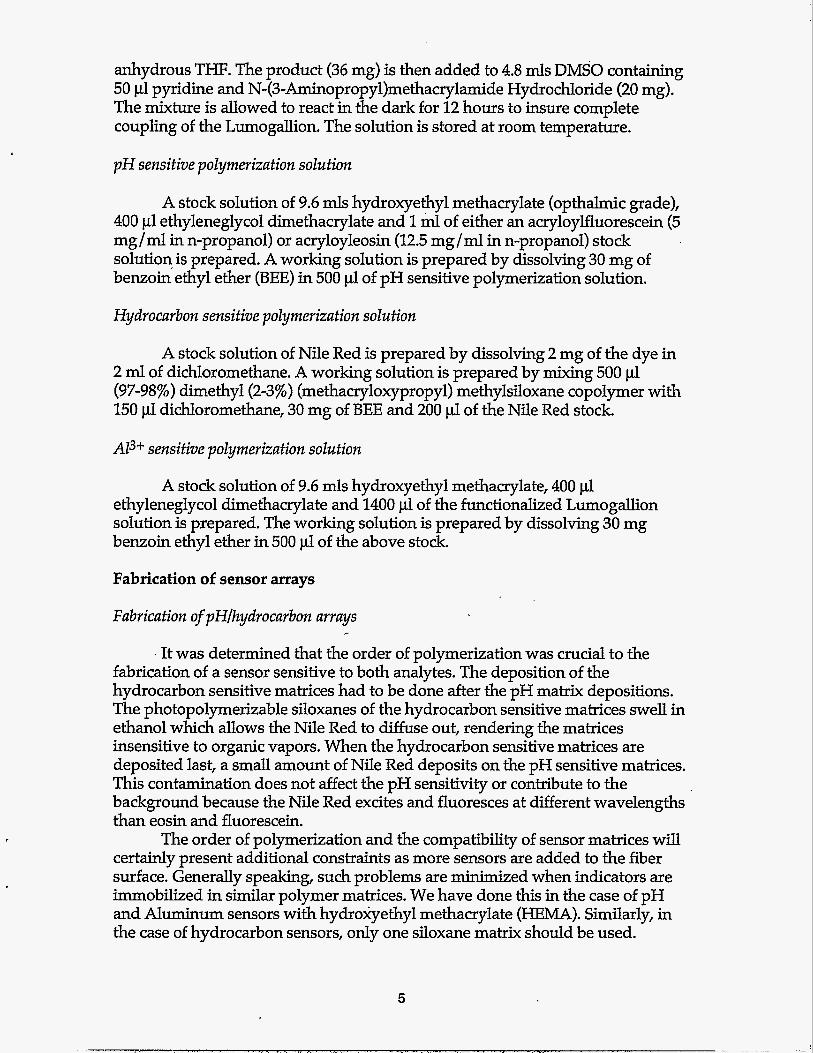
Sensors were tested using the LLNL prototype imaging fluorimeter shown in Figure 4. This prototype instrument will ultimately lead to a field unit. The light source is a 20 Watt halogen bulb followed by a bandpass filter chosen to match the excitation spectrum of the polymer under test. The excitation light is

Figure 4. Concept diagram for a portable, multianalyte fluorimeter and fiber optic sensor.

focused onto the proximal end of the fiber sensor. The amount of light injected into the fiber is measured by collecting the light through the thin polymer into a silicon detector. The input excitation power is measured in order to compare the responsivity of different sensors. The light emitted from the polymer is reflected off a beamsplitter and imaged onto a charge coupled device (CCD) detector at a magnification of 5x. htegration times are typically 1 or 2 seconds.

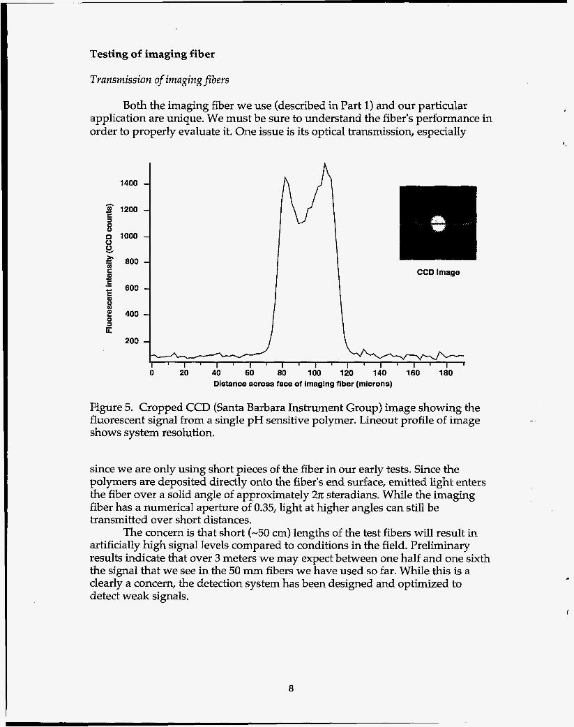
Two different CCD detectors were used during these studies. The first was a liquid nitrogen cooled CCD from Princeton Instruments, Model LNCCD with an 1152 x 298 array of 23.5 pm by 23.5 p m pixels. More recently, we have switched to a thermoelectric cooled CCD from Santa Barbara Instrument Group (SBIG). This detector system is significantly smaller and less expensive than the sophisticated Princeton instrument. At the same time however, it perfonns as well or better in our application. The elements in the 320 by 240 pixel array are 10 pm by 10 pm. The inset in Figure 5 shows a fluorescent image of a single 40 pm diameter pH polymer taken with the SBIG camera. The lineout profile plot shows the resolution of the imaging system to be less than 10 p.

7

Testing of imaging fiber

Transmission of imagingfibers

Both the imaging fiber we use (described in Part 1) and our particular application are unique. We must be sure to understand the fiber's performance in order to properly evaluate it. One issue is its optical transmission, especially

1400

CI

$I 1200

0 1000 0 c 2 800

d + 600

c

8

u) C

C .-

i ?! 400

G 200

-

-

-

-

-

l ~ l ~ l ~ l ' l ~ l ~ l ' l ~ l ~ l ~ 0 20 40 60 80 100 120 140 160 180

Distance across face of imaging fiber (microns)

CCD Image

Figure 5. Cropped CCD (Santa Barbara Instrument Group) image showing the fluorescent signal from a single pH sensitive polymer. Lineout profile of image shows system resolution.

since we are only using short pieces of the fiber in our early tests. Since the polymers are deposited directly onto the fiber's end surface, emitted light enters the fiber over a solid angle of approximately 2n steradians. While the imaging fiber has a numerical aperture of 0.35, light at higher angles can still be transmitted over short distances.

artificially high signal levels compared to conditions in the field. Preliminary results indicate that over 3 meters we may expect between one half and one sixth the signal that we see in the 50 mm fibers we have used so far. While this is a clearly a concern, the detection system has been designed and optimized to detect weak signals.

The concern is that short (-50 cm) lengths of the test fibers will result in

Crosstalk between polymers in a multianalyte sensor

The Sumitumo imaging fibers we are using exhibit very low levels for crosstalk between adjacent channels. This is due to manufacturing techniques which purposely vary the shape of individual channels to frustrate coupling between modes in adjacent fibers.3r4 In addition to the fiber's inherent crosstalk performance, the polymers must be deposited cleanly to avoid overlapping areas. The photodeposition system delivered to Tufts (described in Part 1) was specifically designed to do this.

The profile plot in Figure 5 shows that crosstalk should be negligible. It should be noted that this evaluation corresponds to the worst case condition of neighboring polymers emitting light at identical wavelengths. In general, neighboring polymers will be fluorescing at different wavelengths and their signals will be severely attenuated by the color filters in the imaging fluorimeter.

Testing of pH sensors with portable fluorimeter

Signal level

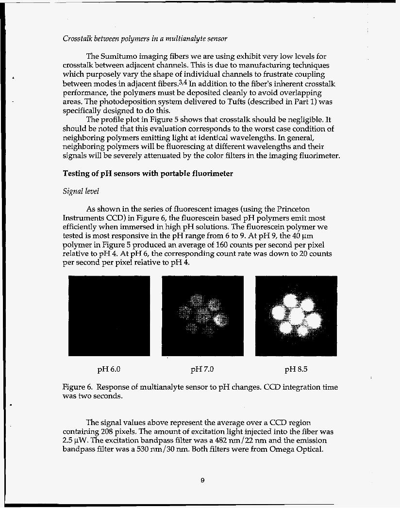
As shown in the series of fluorescent images (using the Princeton Instruments CCD) in Figure 6, the fluorescein based pH polymers emit most efficiently when immersed in high pH solutions. The fluorescein polymer we tested is most responsive in the pH range from 6 to 9. At pH 9, the 40 pm polymer in Figure 5 produced an average of 160 counts per second per pixel relative to pH 4. At pH 6, the corresponding count rate was down to 20 counts per second per pixel relative to pH 4.

pH 6.0 pH 7.0 pH 8.5

Figure 6. Response of multianalyte sensor to pH changes. CCD integration time was two seconds. .

The signal values above represent the average over a CCD region containing 208 pixels. The amount of excitation light injected into the fiber was 2.5 pW. The excitation bandpass filter was a 482 nm/22 nm and the emission bandpass filter was a 530 nm/30 run. Both filters were from Omega Optical.

9

Noise level

The image obtained while the sensor was in a solution of pH 4 was used as the background image for analysis because the fluorescence level is known to be near zero. Using this image also serves to subtract out any scattered light or systematic fluorescence from regions other than the polymer itself. When subtracting such an image from one (nominally) just like it, the mean number of noise counts was less than 1 count/sec/pixel.

Resolution

Over a two second integration time, the emission signal from a pH 7 solution generates 80 more counts per pixel than a pH 6 solution. Even without a zero point reference, these levels are reproducible to within 12%. Measurements were made on a relatively small (40 pm diameter) polymer. If an 80 pm polymer was used, the signal levels might be expected to increase by 4 times (the ratio of their areas). The actual increase would probably be more since it is the increase in polymer volume that matters and the polymers typically have a domed structure (Figure 1).

Other methods for improving the resolution include averaging several images together or integrating for a longer time to accumulate larger signals. These are both operationally valid options due to the fast response time of the sensors. This system should have no difficulty achieving a pH resolution of 0.01 pH unit.

Response time

Generally speaking, the pH sensor responds fully in about 30 seconds, a speed which is fast enough so as not to be a critical issue. In the worst case (chemically slowest) situation of going from pH 4 to pH 9, the sensor reached 89% of its final value in 11 seconds.

signals, they will also respond more slowly. This is because it takes longer for hydrogen ions to diffuse throughout the larger volume.

It should be noted that while thicker polymers will produce stronger

Aging efects

After using the pH sensors over a period of three to five months, we noticed a drop in signal level to as low as one quarter of the original value. However, any aging effect may be complicated by the sensor's recent history, such as whether the fiber was soaking in a neutral solution beforehand or if it was cycled through various pH ranges before final measurements were made. Such effects may account for week to week variations in signal level of a factor of two. One positive note is that during routine testing, these polymers showed no sign of photo-bleaching over a 30 minute period of constant illumination.

HEMA and siloxanes are cell adhesion resilient (siloxanes are used for artificial Although microbes will likely grow on the polymers eventually, both

.

10

arteries). Any effects would probably be small and not result in any damage to the polymers. Proper calibration before use should mitigate these concerns, as well as concerns related to operation under elevated temperatures, etc.

can be refreshed or preserved in any way when not in use. While aging effects are of some concern, they are not a critical issue at this time. In fact, even our oldest sensors are still performing well enough to make accurate measurements if they are calibrated before use.

At this point, we do not know why the polymers degrade or whether they

Testing of hydrocarbon sensors with the portable fluorimeter

We ran preliminary tests on six different polymers that were designed to be sensitive to hydrocarbons. The test compared the signal received when placed above a container of acetone to the signal received when in open air. Absolute signal levels were monitored as well as the percent increase in signal when over acetone. We refer to this ratio as the polymer's efficiency. Of the six polymers tested, three responded with efficiencies of between 20% and 30%.

Signal level

Each of the six polymer types was used to make two separate sensors. In general, these nominally identical sensors exhibited significantly different results. The complete set of preliminary results is shown in Table 1. The excitation bandpass filter was a 530 nm/30 nm and the emission bandpass filter was a 600 m/40 nm. Both filters were from Omega Optical. In these acetone exposures, the PS851 sensor performed better than the PS802 sensor. (The reverse was found to be true at Tufts when tested with dichloromethane.)

Response time and photo-bleaching effects

The response time of these sensors was generally in the range of 30 seconds to one minute. However, unlike the pH sensors, these hydrocarbon sensors may exhibit a noticeable bleaching effect which results in a.peak in the signal (when polymer stabilized) followed by a slow drop in signal. In one PS851 sensor, when the excitation lamp was turned off for a few hours and then restarted, the fluorescence level picked up exactly where it left off, indicating that the photo-bleaching effect was permanent (Figure 7).

Laboratory testing of pHJhydrocarbon array aLTufts

This is the only sensor that has been tested to date that was truly multianalyte. It contained three pH sensitive matrices using eosin, two pH sensitive matrices using fluorescein and two hydrocarbon sensitive matrices, of two different photopolymerizable siloxanes. The proximal end of the array was mounted in the Tufts imaging instrument (Figure 3). The hydrocarbon sensitive matrices were tested by monitoring the fluorescence at 600 run with a 10 nm

11

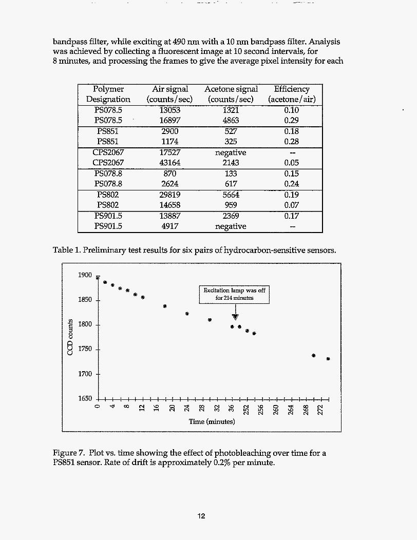
bandpass filter, while exciting at 490 nm with a 10 nm bandpass filter. Analysis was achieved by collecting a fluorescent image at 10 second intervals, for 8 minutes, and processing the frames to give the average pixel intensity for each

Polymer Air signal Acetone signal Efficiency Designation (countslsec) (counts/sec) (acetone/air)

PS078.5 13053 1321 0.10 PS078.5 . 16897 4863 0.29 PS851 2900 527 0.18 PS851 1174 325 0.28

CPS2067 43164 2143 0.05 PS078.8 870 133 0.15 PS078.8 2624 617 0.24 PS802 29819 5664 0.19 PS802 14658 959 0.07

PS901.5 13887 2369 0.17 PS901.5 4917 negative -

CPS2067 17527 negative 1

Table 1. Preliminary test results for six pairs of hydrocarbon-sensitive sensors.

Figure 7. Plot vs. time showing the effect of photobleaching over time for a PS851 sensor. Rate of drift is approximately 0.27% per minute.

12

sensing region with IPLab imaging software. CH2C12 vapors were introduced at- the sensing surface by passing N2 through CH2C12 and passing the saturated N2 stream directly across the fiber surface. The setup for introducing vapors could be switched between pqre N2 and CH2C12 saturated N2 so that response times could be measured.

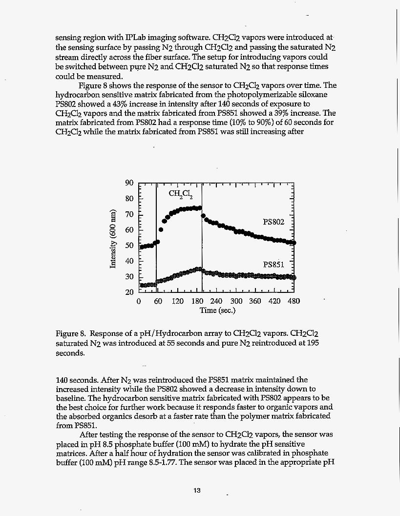
hydrocarbon sensitive matrix fabricated from the photopolymerizable siloxane PS802 showed a 43% increase in intensity after 140 seconds of exposure to CH2Cl2 vapors and the matrix fabricated from PS851 showed a 39% increase. The matrix fabricated from PS802 had a response time (10% to 90%) of 60 seconds for CH2C12 while the matrix fabricated from PS851 was sti l l increasing after

Figure 8 shows the response of the sensor to CH2C12 vapors over time. The

90

80

1 70

8 60 E .g 50 2 3 40

30

20 0 60 120 180 240 300 360 420 480

Time (sec.)

Figure 8. Response of a pH/Hydrocarbon array to CH2C12 vapors. CH2C12 saturated N2 was introduced at 55 seconds and pure N2 reintroduced at 195 seconds.

140 seconds. After N2 was reintroduced the PS851 matrix maintained the increased intensity while the PS802 showed a decrease in intensity down to baseline. The hydrocarbon sensitive matrix fabricated with PS802 appears to be the best choice for further work because it responds faster to organic vapors and the absorbed organics desorb at a faster rate than the polymer matrix fabricated from PS851.

After testing the response of the sensor to CH2C12 vapors, the sensor was placed in pH 8.5 phosphate buffer (100 mM) to hydrate the pH sensitive matrices. After a half hour of hydration the sensor was calibrated in phosphate buffer (100 mM) pH range 8.5-1.77. The sensor was placed in the appropriate pH

13

buffer and allowed to equilibrate for 1 minute. After equilibration a fluorescent image was collected and then the sensor was allowed to equilibrate in the next buffer. Fluorescence was monitored at 530 nm with a 30 nm bandpass filter using 490 nm excitation with a 10 nm bandpass filter. The frames were processed to give the average pixel intensity for each sensing region with IPLab imaging software.

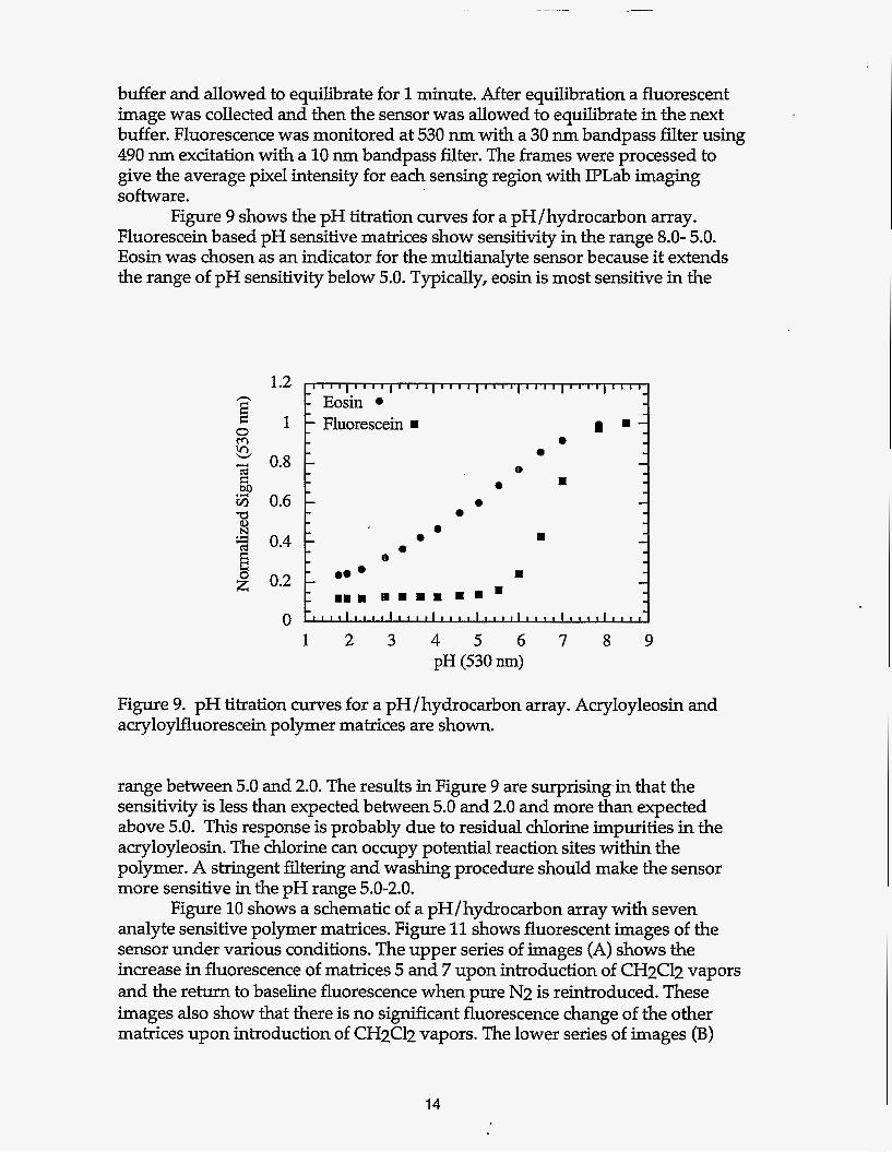
Figure 9 shows the pH titration curves for a pH/hydrocarbon array. Fluorescein based pH sensitive matrices show sensitivity in the range 8.0- 5.0. Eosin was chosen as an indicator for the mdtianalyte sensor because it extends the range of pH sensitivity below 5.0. Typically, eosin is most sensitive in the

1.2

1

0.8

0.6

0.4

0.2

0

0 0

0 0

0 0

0 . 0 .

Figure 9. pH titration curves for a pH/hydrocarbon array. Acryloyleosin and acryloylfluorescein polymer matrices are shown.

range between 5.0 and 2.0. The results in Figure 9 are surprisingin that the sensitivity is less than expected between 5.0 and 2.0 and more than expected above 5.0. This response is probably due to residual chlorine impurities in the acryloyleosin. The chlorine can occupy potential reaction sites within the polymer. A stringent filtering and washing procedure should make the sensor more sensitive in the pH range 5.0-2.0.

Figure 10 shows a schematic of a pH/hydrocarbon array with seven analyte sensitive polymer matrices. Figure 11 shows fluorescent images of the sensor under various conditions. The upper series of images (A) shows the increase in fluorescence of matrices 5 and 7 upon introduction of CH2C12 vapors and the return to baseline fluorescence when pure N2 is reintroduced. These images also show that there is no significant fluorescence change of the other matrices upon introduction of CH2C12 vapors. The lower series of images (B)

14

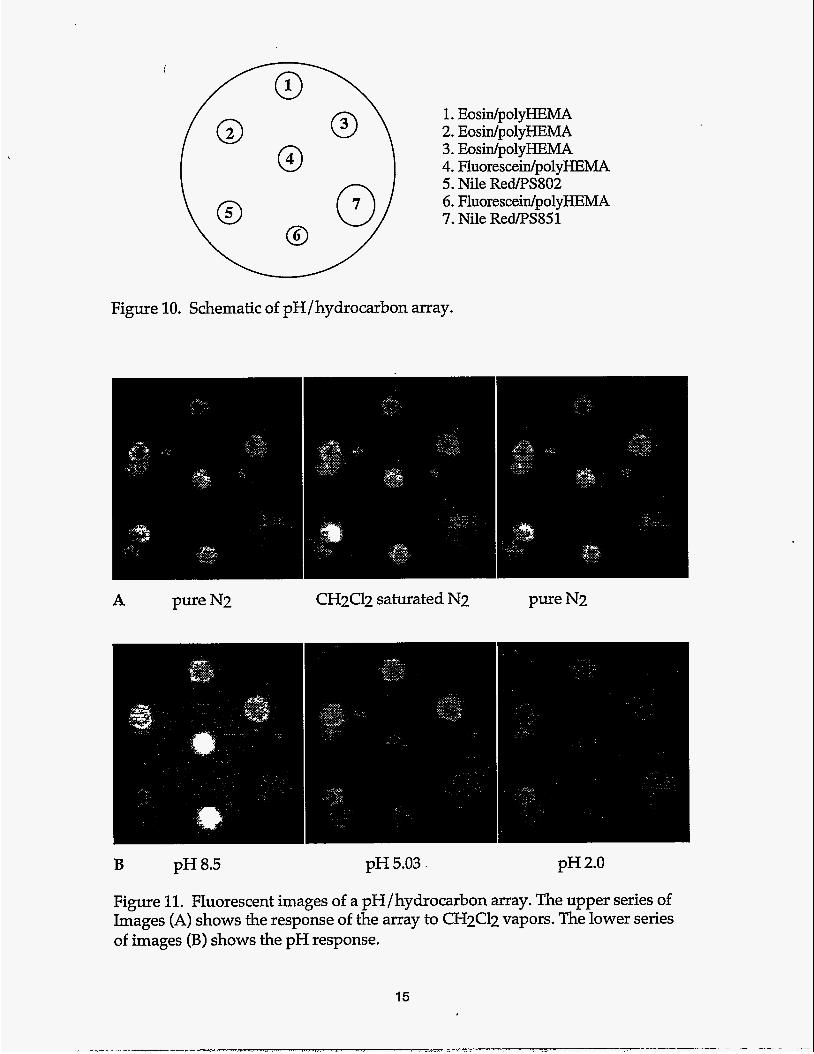
1. EosidpolyHEMA 2. EosidpolyHEMA 3. EosidpolyHEMA 4. Fluoresceidpo1yHEM.A 5. Nile Rems802 6. Fluoresceidpo1yHEM.A 7. Nile RedPS851

Figure 10. Schematic of pH/hydrocarbon array.

B pH8.5 pH 5.03 pH 2.0

Figure 11. Fluorescent images of a pH/hydrocarbon array. The upper series of Images (A) shows the response of the array to CH2C12 vapors. The lower series of images (B) shows the pH response.

15

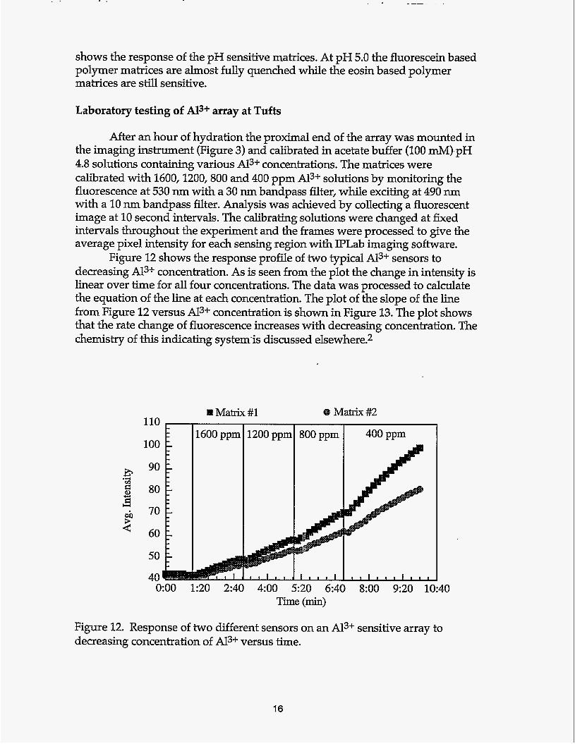
shows the response of the pH sensitive matrices. At pH 5.0 the fluorescein based polymer matrices are almost fully quenched while the eosin based polymer matrices are still sensitive.

Laboratory testing of Al3+ array at Tufts

M e r an hour of hydration the proximal end of the array was mounted in the imaging instrument (Figure 3) and calibrated in acetate buffer (100 mM) pH 4.8 solutions containing various A I S + concentrations. The matrices were calibrated with 1600,1200,800 and 400 ppm A$+ solutions by monitoring the fluorescence at 530 nm with a 30 nm bandpass filter, while exciting at 490 nm with a 10 nm bandpass filter. Analysis was achieved by collecting a fluorescent image at 10 second intervals. The calibrating solutions were changed at fixed intervals throughout the experiment and the frames were processed to give the average pixel intensity for each sensing region with IPLab imaging software.

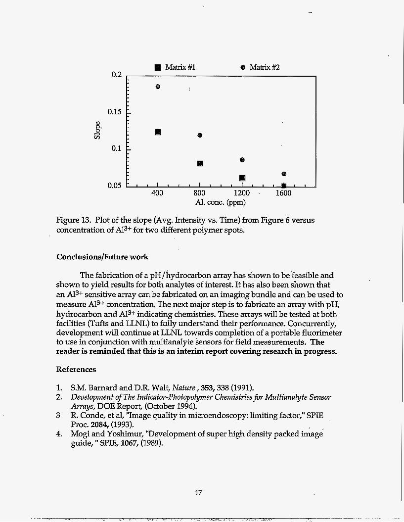
Figure 12 shows the response profile of two typical Al3+ sensors to decreasing Al3+ concentration. As is seen from the plot the change in intensity is linear over time for al l four concentrations. The data was processed to calculate the equation of the line at each concentration. The plot of the slope of the line from Figure 12 versus Al3+ concentration is shown in Figure 13. The plot shows that the rate change of fluorescence increases with decreasing concentration. The chemistry of this indicating system is discussed elsewhere.2

110

a .r(

C

RI Matrix #1

1600 ppm 1200 ppm

Matrix #2

800 ppm I 400 ppm

0:OO 1:20 2:40 400 5:20 6:40 8:OO 9:20 10:40 Time (min)

Figure 12. Response of two different sensors on an Al3+ sensitive array to decreasing concentration of Al3+ versus time.

16

Matrix#l Matrix #2

Figure 13. Plot of the slope (Avg. Intensity vs. Time) from Figure 6 versus concentration of Al3+ for two different polymer spots.

Conclusions/Future work

The fabrication of a pH/hydrocarbon array has shown to be feasible and shown to yield results for both analytes of interest. It has also been shown that an Ala+ sensitive array can be fabricated on an imaging bundle and can be used to measure Al3+ concentration. The next major step is to fabricate a n array with pH, hydrocarbon and Al3+ indicating chemistries. These arrays will be tested at both facilities (Tufts and LLNL) to fully understand their performance. Concurrently, development will continue at LLNL towards completion of a portable fluorimeter to use in conjunction with multianalyte sensors for field measurements. The reader is reminded that this is an interim report covering research in progress.

References

1. 2.

3

4.

S.M. Barnard and D.R. Walt, Nature, 353,338 (1991). Development of The Indicator-Photopolymer Chemistries for Multianalyfe Sensor Arrays, DOE Report, (October 1994). R. Conde, et al, "Image quality in microendoscopy: limiting factor," SPE Proc. 2084, (1993). Mogi and Yoshimur, "Development of super high density packed image guide, I' SPIE, 1067, (1989).

17