Product Market Regulation, Trend Inflation andInflation Dynamics in the New Keynesian Phillips

Curve

Laurence Bloch ∗†‡§

23 June, 2009

Abstract

In this empirical paper, we take a close look at the impact of observed changes in theproduct market regulation, which raises barriers to entry and empediments to competition,on inflation dynamics since the early 1980s.We use an enlarged new Keynesian Phillips curve (NKPC) allowing for entry of firms and

for increasing competitive pressures with the number of firms and non zero trend inflation.Using OECD indicators on product market regulations, characterized by persistent fluc-

tuations of their underlying trends, and taking into account the non stationary propertiesof the inflation process, we investigate the empirical relevance of this NKPC for inflationdynamics in the US and France, with the additional assumption that shifts in monetaryinflation target are related to changes in the product market regulation. We also assumeVAR expectations. The results point out that product market regulation is a good candidateas an exogenous structural source of the observed persistence in inflation for the last thirtyyears in both the US and France.Keywords: Firm entry, Product market regulation, New Keynesian Phillips Curve, Trend

inflation, Inflation dynamics, VAR.JEL Classification: E31 .

∗CREST-INSEE, TJ310, 15, boulevard Gabriel Péri - 92245 Malakoff Cedex - France, tel:+33 (0)1 41 17 6034, Email: laurence.bloch@ensae.fr

†The views expressed herein are those of the author and do not reflect the position of INSEE.‡We thank Guillaume Chevillon, Stéphane Grégoir, Guy Laroque, Hervé Le Bihan, and participants in the

Macroeconometrics CREST Seminar and in the AFSE Congress 2008 for useful discussions.§This version is a modified version of a preliminary draft (September 12, 2008) presented at the AFSE Congress

2008.

1

1 Introduction

In this empirical paper we investigate in which extent the interaction between costs of entryon the product market which raises barriers to entry and empediments to competition and shiftsin the long-run inflation target can account for lag dynamics and persistence in inflation sincethe early 1980s, using the New Keynesian Phillips Curve (NKPC) framework. We explicitlytake in account the non-stationary properties of the inflation process but also those of theOECD indicator for product market regulation and costs of entry, characterized by persistentfluctuations of its underlying trend. Our theoretical departure point is a derived NKPC basedon the standard Calvo (1983) optimal price setting with staggered prices, enlarged with a nonzero steady state inflation, but also allowing entry of firms and increasing competitive pressureswith the number of firms (see our companion paper Bloch (2009)).

In its basic form, the Calvo model leads to a purely forward-looking inflation specificationrelating inflation to expected inflation and fluctuations of real marginal costs of production.However, many empirical studies conclude that this version of the NKPC generates too littlepersistence to be consistent with empirical evidence. Consequentely, many authors improvethe empirical fit of the NKPC by adding backward looking elements in the NKPC (the so-called “hybrid NKPC” including backward and forward elements). The justifications of theintroduction of lags of inflation are of different types: a fraction of agents use adaptative insteadof rational expectations (Roberts (1997, 2006), Ball (2000)); the fraction of firms which are notre-optimizing their prices follow an indexation rule on some general price inflation (Christianoet al. (2005)); some firms use rule-of-thumb pricing (Gali and Gerler (1999)); or agents areconcerned with real wage instead of nominal wage (Phelps-Taylor) in a model of overlapping wagecontracts (Fuhrer and Moore (1995)). These justifications have often been criticized because oftheir lack of convincing microeconomic foundation and are considered as ad-hoc.

Over the last years, a few authors have tried to find more founded explanations to persis-tence in macroeconomic variables, in particular inflation. Some authors departed from rationalexpectations and replaced it by learning mechanism. In that case agents do not know the struc-tural parameters of the economy and use historical data to infer parameters: they learn overtime, updating their beliefs. For example, in Milani (2007), using Bayesian method, the empir-ical results showed that learning can represent a potential single mechanism which can inducepersistence without having to invoke indexation in the model. Schorfheide (2005) put forwardlearning of firms and households about monetary policy shifts in the target inflation rate, usinglearning rule to infer the current state of monetary policy and found that actual and expectedinflation in the early 1980 can well be captured by the delayed response of the learning speci-fication. Other authors used learning as a tool that can help in understanding some particularepisodes of US inflation and monetary policy, which are often harder to explain under rationalexpectations. They focused on explanations why monetary policy shifts occur over time and putforward that the Central bank adjusts its target as it learns about the effectivness of its policy(Sargent (1999), Cogley and Sargent (2005), Primiceri (2006), and Sargent, Williams and Zha(2006)).

Recently, Cogley and Sbordone (2008) hypothesized that inflation persistence results mainlyfrom variation in the long-run component of inflation. They argued that the apparent needfor lagged inflation in the NKPC comes from neglecting the interaction between drift in trend

2

inflation and non-linearities in a more exact version of the Calvo model taking into account ashifting steady state associated with a time-varying inflation trend.

The consequences of the assumption of non zero steady state inflation in the derivation ofthe new Keynesian Phillips curve (NKPC) based on Calvo price setting with staggered priceshave already been explored on the theoretical side (King and Wolman (1996), Ascari (2004),Sahuc (2006) and Bakhshi and al. (2007)). The presence of a non zero steady state inflationalters the structure of the NKPC: the coefficients on past and future inflation as well as theslope of the NKPC then become functions of trend inflation. The NKPC then includes anadditional forward-looking inflation variable with a complex structure. Furthermore, the slopeof the NKPC decreases with trend inflation. This implication sits oddly to the stylized factfrom the traditional Phillips curve literature and the conventional wisdom that Phillips curvesare flatter at low inflation levels. To avoid these implications, Sahuc (2006) and Bakhshi andal. (2007) showed that the decrease of the slope with trend inflation can be weakened, evenoffset, through partial backward indexation of prices for firms, which do not reoptimize theirprices in the Calvo price-setting, or through the frequency of price adjustment (Calvo priceadjustment signal) becoming an inverse function of the trend inflation rate. On their side,Cogley and Sbordone (2008) were recently the first to provide an empirical estimation of theNKPC with a time varying inflation trend. Following Sbordone (2002, 2005) and Fanelli (2008),they estimated the model in two steps: first, estimating a Bayesian unrestricted VAR withdrifting parameters and stochastic volatility; second, estimating the parameters of the pricingby exploiting cross-equations restrictions on the VAR parameters. Their estimations pointedout that the backward-looking indexation parameter concentrates on zero and that indexationappears to be unnecessary once drift in trend inflation is taken into account. The weight offuture expectations is enhanced as trend inflation increases. However, Cogley and Sbordoneestimations went on exhibiting a muted slope with increase in trend inflation, and thus anincreasing slope since the beginning of the 1980s which is at odds with stylized facts. Moreover,they attributed fluctuations in the underlying inflation trend to shifts in monetary policy, butwithout testing this assertion. Previously, Kozicki and Tinsley (2002) had already put forwardthat shifts in “the anchor of long horizon inflation expectations” can be a potential source oflag dynamics in inflation. They estimated a multivariate VAR with shifting endpoints wherethe only source of non stationarity directly derives from shifts in the steady state. Besides,Ireland (2007) tried to draw inferences about the behavior of the Fed’s unobserved inflationtarget, looking closely at both assumptions: inflation target movements are deliberate policyresponse to exogenous supply-side shocks hitting the economy and movements in inflation targetare purely random. He found that both interpretations are statistically indistinguishable andconcluded that considerable uncertainty remains about the true source of shifts in the inflationtarget.

In this paper, building on the hypothesis of a non zero steady state inflation and time-varyinginflation trend, we make the additional assumption that trend in inflation arises from shifts inthe exogenous process of the product market regulation. Through this last assumption, we followIreland (2007) and the growing literature (already mentioned) assuming that the Central Banklearns from the structure of the economy. Our theoretical model is based on the NKPC with anon zero steady state inflation, but also allowing for entry of firms regulated by costs of entryand non fixed number of varieties, assuming a one to one identification between a producer, adifferentiated good product and a firm. The elasticity of demand faced by firms and competitive

3

pressures also increase with the number of varieties. This enlarged NKPC exhibits the followingproperties: 1) in the long run, real average marginal cost decreases with inflation, but this effectis enhanced in an economy where the cost of entry for firms is low; real average marginal costalso increases with the number of varieties; 2) in a context of decreasing trend inflation, thecoefficients of the NKPC can be stabilized through the increase of competitive pressures andthat of the elasticity of the demand faced by the firms, both implied by an increase in thetendency in the number of varieties. Thus, without referring to an increase in partial indexationor to an endogenous price rigidity, we reconcile theory with stylized facts (Bloch, 2009).

Bilbiie and al. (2007) have already put forward that net entry of firms induces an extra termlinked to the fluctuations of the number of firms around the steady state and that this variablewould take a part of the observed persistence in the dynamics of product price inflation in theNKPC. However, we argue that fluctuations of the number of firms, an a priori stationaryvariable, is empirically not a good candidate to match the observed persistence in inflation.Besides, increasing competition in the long run would contribute theoretically to flatten theslope of the traditional Phillips curve. However, empirical investigations focusing on the impactof globalization on the slope of the Phillips curve are rather inconclusive or provide contradictoryconclusions1: Borio and Filardo (2007) empirically supported for many countries a “global slack”hypothesis since 1993, according to which the decline in the sensitivity of inflation to output gapcan be explained by the fact that global measures od demand pressure have become the maindriving force of inflation dynamics. Ihrig and al. (2007) questioned the global slack hypothesis,the latter not being robust to the specification of the measures of global slack. Finally, Ball(2006) allowed interaction of the output coefficient with trade in a traditional Phillips curvethat was estimated for the US only and found only a modest effect. Sbordone (2008) putforward that globalization increases the elasticity of demand faced by firms, but decreases theelasticity of the desired mark-up; hence, globalization decreases the slope of the NKPC only forlarge enough increases in the number of good traded.

We investigate the empirical relevance of our derived NKPC for inflation dynamics with theadditional assumption that shifts in monetary inflation target originate from product marketregulation’s ones. In the same vein as Cogley and Sbordone (2008) or Cogley and al. (2008) forthe inflation process, we take also into account the stochastic trend in the number of varietiesand estimate an empirical version of our enlarged NKPC assuming VAR expectations. FollowingSbordone (2002, 2005), Fanelli (2008) and Cogley and Sbordone (2008) we estimate the modelin two steps, first estimating an unrestricted VAR, and then estimating the NKPC by exploitingcross-equations restriction on the VAR parameters. We restrict the empirical evidence to twocountries: the US and France, the first one is representative of the anglo-saxon area, flexible andwhere large reforms in the product market regulation have already been conducted during thelast thirty years, the second is representative of the euro area, less flexible and where changes inthe product market regulation started ten years later, from the late 1980 and are still in progress.The OECD indicators on product market regulation are characterized by high persistence comingfrom their underlying trend.

On one hand, we address the issue of potential misspecification of the basic NKPC modelin case of omitted variables by taking into account the entry of firms through the productmarket regulation variable. To our knowledge, the recent empirical papers (already mentioned)

1See also Mishkin (2007, 2008), Roberts (2006).

4

on this topic (Batini and al.(2005), Borio and Filardo (2007), Ball (2006), Ihrig and al. (2007)and Sbordone (2008)) have focused on the impact of globalization and increased global marketcompetition on inflation, rather than on the impact of product market regulation.

On the other hand, through the link between stochastic trend inflation and product marketregulation (behaviour of the Central Bank), we generate an exogenous structural source ofpersistence and thus we address the question of the observed inflation persistence in a forwardlooking model of inflation. Our econometric results show that the introduction of the productmarket regulation variable takes a part of the observed persistence in inflation and lowers theestimate of the partial indexation and hence of the backward looking component of inflation.Moreover, changes in product market regulation have a greater impact in the long run on trendinflation in the US than in France.

This paper is organized as follows. The next section gives the derived NKPC, extended tothe cases of trend inflation with entry of firms and increasing competitive pressures with thenumber of firms. Section 3 assesses the empirical relevance of empirical versions of this NKPCfor inflation dynamics for the US and France and discusses the robustness of the results.

2 The Model

Our empirical investigation is based on a new Keynesian (NK) model allowing endogenousnumber of producers of goods. We assume exogenous entry costs and firms enter instantaneouslyin each period until all expected profit opportunities are exploited. Nominal rigidities are intro-duced in the form of staggered price setting by firms using the formalism due to Calvo (1983).The NKPC is then derived, under entry of firms and in addition with elasticity of demandand competitive pressures increasing with the number of firms; the log-linearization around thesteady state takes into account the non zero steady state inflation (for more details, see Bloch(2009)).

2.1 The enlarged NKPC with non zero steady state, entry of firms and in-creasing competitive pressure with number of firms

Our objective is to offer a structural explanation of the observed inflation persistence,allowing fluctuations both in the inflation trend and in the costs of entry tendency. Hencewe depart from the traditional derivation of the Calvo model which assumes constant steadystate and approximation (by log-linearization) of the equilibrium conditions of the Calvo pricingmodel around the steady state.

Thus at each period t, each firm, new entrant or pre-existing firm, behaves in maximizingtheir expected sum of profits as if it has perfect information on steady state values of grossinflation rate Πt, number of products Nt and entry costs fEt and as if these steady state valuesare fixed in the future to constant values, respectively Πt, N t, fEt.

We assume that the Central Bank conducts monetary policy according to a generalizedTaylor rule where the Central Bank increases the short term nominal interest rate whenever theinflation rate rises above its target Πt. Following Ireland (2007) the time-varying inflation targetΠt evolves according to the rule:

Πt = α1fEt + α2 (1)

5

This addition to the Taylor rule allows the Central Bank to adjust its inflation target inresponse to exogenous shocks to product market regulation. On their side, when optimizing,firms and consumers do not know this target rule.

Allowing for time-varying stochastic trends in inflation and in number of varieties has adirect consequence: when approximating the non-linear equilibrium conditions of the model,we take the log-linear approximation, in each period t, around a steady state associated withtime-varying trends Πt and N t respectively in inflation and in number of varieties.

Finally, contrary to some authors (see for example Sims and Zha (2006)) we do not treat thechange from one equilibrium to another as probabilistic.

Hence, at each period t, the equilibrium inflation is defined by the following local approxi-mation2:

bπt−%bπt−1 = −%bgπt +γ( bNt−1−bgNt )− γϕ0t

1− αΠ(1−%)(θ(Nt)−1)t

bNt+ϕ2t%Etcgπt+1−γϕ2t( bNt−EtcgNt+1)+...

...γϕ2tϕ0t

1− αΠ(1−%)(θ(Nt)−1)t

Et bNt+1 + ϕ4tcmct + ϕ4t((γ(θ(N t)− 1)− 1)(ω + ξ(N t)) bNt − ϕ4t(1− a)

bDt

...+ β1tEt(bπt+1 − %bπt) + β2tEt

∞Xj=2

ϕj1(bπt+j − %bπt+j−1) + β3tEt

∞Xj=0

ϕj1(bqt+j,t+j+1 + bgyt+1+j) (2)with the long run restriction between trend inflation Πt, trend number of firms N t and trend

real average marginal cost mct:

(1/mct) =

⎡⎢⎢⎣⎛⎝1− αΠ

(1−%)(θ(Nt)−1)t

1− α

⎞⎠1−θ(Nt)1+θ(Nt)ω

⎤⎥⎥⎦⎡⎣ θ(N t)

θ(N t)− 1

⎛⎝ 1− αqgygbθ(Nt)−1Π

(1−%)(θ(Nt)−1)t

1− αqgygbθ(Nt)−1Π(1−%)θ(Nt)(1+ω+ξ(Nt))t

⎞⎠⎤⎦ ...

...

∙D

−1(1−a)t N

−γ(Nt)(1+ω)−ωt

¸(3)

2With the coefficients defined by:

ϕ0t=

1−αΠ(1−%)(θ(Nt)−1)t

αΠ(1−%)(θ(Nt)−1)t

ϕ1t = αqgygbθ(Nt)−1Π

(1−%)(θ(Nt)−1)t

ϕ2t = αqgygbθ(Nt)−1Π

(1−%)θ(Nt)(1+ω+ξ(Nt))t

ϕ3t = 1− ϕ2tβ1t = ϕ2t(1 + ϕ0t) +

ϕ0t(1+θ(Nt)(ω+ξ(Nt))

(ϕ2t−ϕ1t)ϕ1t

(θ(N t)− 1)ϕ1tβ2t =

ϕ0t(1+θ(Nt)(ω+ξ(Nt))

(ϕ2t−ϕ1t)ϕ1t

(θ(N t)− 1)β3t =

ϕ0t(1+θ(Nt)(ω+ξ(Nt))

(ϕ2t−ϕ1t)ϕ1t

ϕ1tϕ4t =

ϕ0t(1+θ(Nt)(ω+ξ(Nt))

ϕ3t.

6

The long run restriction (3) is one of the five equations summarizing the steady state where

number of firms N t, real average marginal cost mct, aggregate output Y t, real wage³WtPt

´and

relative price dispersion Dt are determined in function of trend inflation Πt and trend costs ofentry fEt (see appendix). Moreover, the target inflation rule (1) is added.

Hatted variables denote log deviation from trend values and a bar over a variable indicatesits trend value. Thus, bπt denotes log deviation of inflation from its trend value Πt, cmct logdeviation of average real marginal cost, bNt log deviation of the number of varieties 3. Theequation (2) differs from conventional versions of the NKPC in two respects. First, a numberof additional variables appear on the right-hand side of (2). These include higher-order leads ofexpected inflation, innovations to trend inflation, terms involving the real discount factor andreal output growth and also deviations of the number of varieties (instantaneous, lag and lead).Second, the coefficients of the variables are non linear functions of the trend values of the grossrate of inflation Πt and of the number of varieties N t and of structural parameters of the NKmodel, α the nominal price rigidity, % the backward partial indexation, 1 − a the elasticity ofthe production relatively to labour, ω which measures the extent of strategic complementarity,and θ(N t), ξ(N t), γ(N t), respectively the elasticity of substitution, the elasticity of the mark-upand the consumer taste for variety at their steady state values.

First, in the long run, real average marginal cost decreases with inflation, but this effect isenhanced in an economy where the cost of entry for firms is low; real average marginal costalso increases with the number of varieties. Second, the increase of the slope with decreasingtrend inflation can be alleviated, even inverted, by the decrease of the slope in the tendencyof the number of varieties because of increasing elasticity of substititution of demand with thenumber of varieties, without referring to an increase in partial indexation or an endogenous pricerigidity. The impact of expectations of inflation farther in the future is not only enhanced astrend inflation increases but also with the tendency of the number of varieties. Therefore, in acontext of decreasing trend inflation, the coefficients of the NKPC can be stabilized through theincrease of competitive pressures and that of the elasticity of the demand faced by the firms,both implied by an increase in the tendency in the number of varieties.

2.2 A simplified version of the enlarged NKPC

Omitting the fluctuations of the number of varieties around their steady state values andwith a quite small coefficient β3, we henceforth derive a simplified version of (2):

bπt − %bπt−1 = ϕ4cmct + β1Et(bπt+1 − %bπt) + β2Et

∞Xj=2

ϕj1(bπt+j − %bπt+j−1) (4)

and its closed form solution:

bπt = %bπt−1 + ϕ4Et

∞Xj=0

βj1cmct+j + β2Et

∞Xk=0

βk1

∞Xj=2

ϕj1(bπt+k+j − %bπt+k+j−1) (5)

with the long run restriction (3) between N t, Πt and mct and the target inflation rule (1).3Specifically, bπt = ln(Πt/Πt), cmct = ln(mct/mct), bNt = ln(Nt/N t), bgπt = ln(Πt/Πt−1), bgyt = ln(gyt /g

y),bqt,t+1 = ln(qt,t+1/qt,t+1) with qt,t+1 the real discount factor between time t and t+ 1.7

Henceforth, in a context of decreasing trend inflation but increasing number of varieties, weassume that the coefficients of this NKPC are constant.

3 Econometric Approach

3.1 Characterizing inflation, growth of real GDP and product market regu-lation processes

According to the literature on the “Great moderation” and on the “Inflation stabilization”(see Stock and Watson (2002, 2003, 2005, 2007), Cecchetti and al. (2007), Cogley and Sargent(2005), Cogley and Sbordone (2008), Cogley and al. (2008)), one can start with several postu-lates. (1) The inflation process in the G-7 countries can well be approximated as the sum ofa persistent component and a transitory one. The persistent component captures the stochas-tic trend Πt which evolves as a driftless random walk while the cyclical component representstemporary differences between actual and trend inflation. Because trend inflation is a drift-less random walk, actual inflation has a unit autoregressive root and is highly persistent. (2)Moreover, variability of both the trend and temporary components is allowed to change overtime. This time variation captures the fact that trend inflation has been relatively stable in theG-7 over the past decade, while trend inflation was much more variable in the 1970s (when itrose) and early 1980s (when it fell) in much of the G-7. (3) Real GDP growth rates in the G-7are well characterized, at least locally, by low order autoregressive (AR) models where the ARcoefficients are allowed to drift through time and the volatility of the process is time-varying.

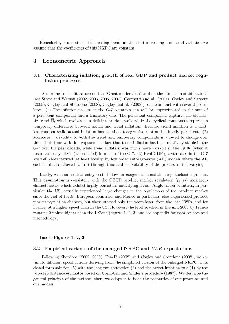
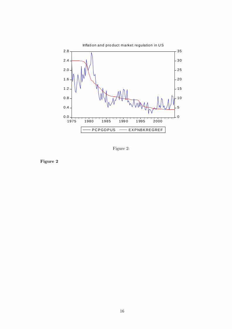
Lastly, we assume that entry costs follow an exogenous nonstationary stochastic process.This assumption is consistent with the OECD product market regulation (pmrt) indicatorscharacteristics which exhibit highly persistent underlying trend. Anglo-saxon countries, in par-ticular the US, actually experienced large changes in the regulations of the product marketsince the end of 1970s. European countries, and France in particular, also experienced productmarket regulation changes, but those started only ten years later, from the late 1980s, and forFrance, at a higher speed than in the US. However, the level reached in the mid-2005 by Franceremains 2 points higher than the US’one (figures 1, 2, 3, and see appendix for data sources andmethodology).

Insert Figures 1, 2, 3

3.2 Empirical variants of the enlarged NKPC and VAR expectations

Following Sbordone (2002, 2005), Fanelli (2008) and Cogley and Sbordone (2008), we es-timate different specifications deriving from the simplified version of the enlarged NKPC in itsclosed form solution (5) with the long run restriction (3) and the target inflation rule (1) by thetwo-step distance estimator based on Campbell and Shiller’s procedure (1987). We describe thegeneral principle of the method; then, we adapt it to both the properties of our processes andour models.

8

3.2.1 The method: estimation by the two-step procedure

We assume that agents form expectations with a forecasting V AR. We use an auxiliaryV AR process, assuming a vector of forecasting variablesXt (n, 1) including at least current grossinflation rate (in logarithm) and the labor share (in logarithm), with a V AR(p) representation:

Xt = A1Xt−1 + ...+ApXt−p + [BWt] + ut

where B is a (n, k) matrix and Wt is a vector (k, 1) of exogenous variables. Wt may bereduced to the constant variable.

The V AR(p) representation can be rewritten as a V AR(1), using the companion matrix Φ:

Zt = ΦZt−1 + [CWt] + Ut

where Zt = (Xt,Xt−1, ...,Xt−p+1)0 (n.p, 1), and

Φ =

⎛⎜⎜⎝A1 A2 ApIn 0 0

0 0 In 0

⎞⎟⎟⎠ (n.p, n.p), with C = (B, 0, ..., 0)0 (n.p, k) and Ut = (ut, 0, ..., 0)0

(n.p, 1)

We write :

πt = e0πZt and mct = e

0mcZt with an appropriate definition of the selection vectors eπ and

emc.

We define the stochastic trend in Zt as the value to which the serie is expected to convergein the long run Zt = limh→∞EtZt+h. Here Zt is defined by Zt = (I − Φ)−1 [CWt] and thus bZtby bZt = Zt −Zt.

The reduced-form conditional expectation of bπt is Et(bπt/ bZt−1) = e0πΦ bZt−1.Similarly, the infinite sum of expected future values of the labor share is computed as:

∞Pj=0

βj1Etcmct+j = e0mc(I − β1Φ)−1Φ bZt−1

and the infinite sum of expectations farther in the future can be written as:

Et

∞Xk=0

βk1

∞Xj=2

ϕj1(bπt+k+j − %bπt+k+j−1) = (I − β1Φ)−1(e0π(ϕ

21(I − ϕ1Φ)

−1(Φ3 bZt−1 − %Φ2 bZt−1))Thus, the conditional expectation of bπt in the model (5) is:

bπst ≡ Et(bπt/ bZt−1) = %e0π bZt−1+ϕ4e0mc((I−β1Φ)−1Φ bZt−1)+β2((I−β1Φ)−1e0πϕ21(I−ϕ1Φ)−1(Φ3 bZt−1−%Φ2 bZt−1)The parameters to be estimated in the NKPC are ψ = (%,ϕ4,β2).

9

After equating reduced-form and structural forecasts of the inflation gap bπt, we obtain a setof non-linear cross-equations restrictions involving the parameters ψ of the model and the V ARparameters Φ and [C]:

e0πΦ − %e0π + ϕ4e0mc((I − β1Φ)

−1Φ) + β2((I − β1Φ)−1e0πϕ

21(I − ϕΦ)−1(Φ3 − %Φ2)) = 0 or

F1(ψ,Φ, [C]) = 0

The parameters must also satisfy the long run restriction (3) between mct,Πt and N t andthe target rule (1) or F2(ψ,Φ, [C]) = 0.

Defining F (ψ,Φ, [C]) by (F1, F2), the minimum distance estimator bψ of ψ = (%,ϕ4,β2)

is defined as the vector that minimizes the square of the function F (ψ, bΦ, [ bC]) for consis-tent estimates of Φ (and [C]) . The minimum distance estimator bψ is then defined as bψ =

argminhF (ψ, bΦ, [ bC])0F (ψ, bΦ, [ bC])i.

The two-step procedure will be: 1) to estimate an auxiliary VAR and consistent estimatesof Φ (and [C]); 2) to estimate the parameters ψ = (%,ϕ4,β2) of the model through a minimumdistance procedure.

3.2.2 Application of the two-step procedure

We apply the two-step procedure to the estimation of three specifications, with two variantsV and V’ for each one, deriving from the closed form solution (5):

Variant V: bπt = %bπt−1 + ϕ4EtP∞j=0 β

j1cmct+j

Variant V’: bπt = %bπt−1+ϕ4EtP∞j=0 β

j1cmct+j+β2EtP∞

k=0 βk1

P∞j=2 ϕ

j1(bπt+k+j−%bπt+k+j−1)

The variant V’ includes the additional variable for the expectation in the future of inflationand thus assumes of a non zero trend inflation. The variant V omits the expectation in thefuture of inflation (the coefficient β2 becomes null) and corresponds to a simplified version of V’;in case of zero trend inflation it corresponds to the usual hybrid NKPC with no time-varyingtrend inflation.

We estimate a trivariate auxiliary V AR of the form Xt = (ln(mct), ln(Πt), gyt)0, with mct

proxied by the labor share, Πt is the gross inflation rate (corrected in the model 3 from its trendthrough a cointegrating relation) and gyt the growth of real GDP. The three models diverge inthe way the product market regulation pmrt is introduced as exogenous variable in the VAR.

In the model 1 the V AR only includes the constant as exogenous variable. The variantV1 corresponds to the usual hybrid NKPC with no time-varying trend inflation and no time-varying number of varieties (in this case, β1 is assumed to be equal to 0.99). The variant V1’corresponds to an approximated hybrid NKPC with time-varying trend inflation as in Cogleyand Sbordorne (2008), but where the coefficients of the VAR are assumed to be constant andthe variables in the NKPC are not taken in deviation of their trend.

In the model 2 the V AR also includes the product market regulation variable as exogenousvariable. The variant V2’ corresponds to the hybrid NKPC incorporating both time-varyingtrend inflation and time-varying number of varieties. Following numerical calculations, in anenvironment of decreasing inflation trend and increasing trend in the number of varieties, we

10

assume that the coefficients β1 and ϕ1 are constant and respectively equal to 1.01 and 0.78; wealso assume ϕ4 and β2 to be constant. The variant V2 corresponds to a simplified version ofV2’.

In the model 3 the V AR doesn’t include the product market regulation as exogenousvariable, because the inflation has already been corrected from its stochastic trend through itscointegrating relation with the product market regulation. It corresponds to a restricted versionof the model 2 or to a specific version of the model 1 where the variable of inflation ln(Πt)isreplaced by its deviation from the monetary inflation target ln(Πt/Πt).

3.2.3 Empirical results

The V AR lag length, 5, has been selected by combining standard information criteria(Akaike, Schwarz, Hannan-Quinn) with residual-based diagnostic tests. In each V AR, the inno-vations for inflation and growth real GDP in the US and in France present stochastic volatilitiesin accordance with the literature (see 3.1). We modelize it with a Garch(1,1), where the repre-sentation of the conditional variance of the residuals εt is expressed as: σ2t = a0 +a1σ

2t−1+a2ε

2t−1.

For each model, in both countries, we test the assumption of constant coefficients of the VARthrough the conditional variance of the residuals specification allowing for the inclusion of thepredetermined regressor exp(pmrt). This inclusion is always rejected.

The non-linear long run restriction (3) between mct,Πt and N t is obviously rejected by thedata in the US and France because the period of estimation exhibits downward trend in theproduct market regulation, in inflation and in real marginal costs. However, both for the USand France, the inflation target rule (1) cannot be rejected at the standard confidence levels:the impact of product market regulation on inflation is greater (multipled by 4.5) in long runfor the US than for France.

In the tables of results (see tables 1 and 2) ln(Π)p indicates the inflation series predicted(static forecasting) by the model, and two statistics measure the approximation of predictedto actual inflation: the ratio of the standard deviations, σln(Π)p/σln(Π) , and the correlationcoefficient, corr(ln(Π)p, ln(Π))4.

For the model 1, in our first step procedure we estimate the baseline unrestricted auxiliaryV AR. For the US, the estimated VAR exhibits no serial correlation of the residuals (only atp=10% for the growth of real GDP) in spite of close to unit roots. This result suggests theexistence of long term relations between the non-stationary variables. Thus, for the US, theleast square estimates of the VAR are consistent. Moreover, the hypothesis that inflation has nopredictive power for the labor share can be rejected at the confidence level p=0.15; the one thatlabor share has no predicive power for inflation can be rejected at the standard confidence levels.For France, the hypothesis that inflation and growth of real GDP have no predictive power forthe labor share cannot be rejected at standard confidence level; the one that inflation has nopredictive power for the growth of real GDP cannot also be rejected at standard confidence level.Furthermore, we obtain serial correlated residuals in the equations of labor share and inflation in

4We should take into account the uncertainty associated with the first step estimate of the V AR parameters,using bootstrap procedure.

11

the V AR with roots of the V AR close to the unit circle. In that case, the least square estimatesof the V AR, bΦ and [ bC], are not consistent.

Using the two step procedure different results emerge: in the model V1, the indexationparameter % estimate is rather high (0.59 for both the US and France). The correlation betweenthe sum of expected value of real marginal costs and inflation is rather high for the US andFrance (resp. 0.81 and 0.86).

The introduction of the expectations of inflation further in the future as additional variablein the second step (model V1’) reduces the estimate of % (from 0.59 to 0.49 for the US and from0.59 to 0.36 for France) and slightly reduces the estimate of the slope: in the US, from 0.0108to 0.0086, and in France from 0.0142 to 0.0133. It seems that the variable of the expectationsof inflation further in the future (very well correlated with inflation, 0.84 in the US and 0.83in France) takes a part of the inflation persistence otherwise taken by the lagged variable bπt−1.For the US, although the least square estimates of the coefficients of the VAR are consistent,the models V1 and V1’ appear to be poorly specified because of the omission of trend variables.

These results confirm the poor empirical performance of the standard NKPC or of the NKPCwith time-varying trend inflation, but assuming constant coefficients in the VAR.

For the model 2, the unrestricted auxiliary V AR includes an additional exogenous vari-able, the product market regulation variable pmrt (in exponential) which presents a persistentunderlying decreasing trend. The product market regulation variable seems to capture a partof the persistence of endogenous variables in the US but not in France. The serial correlationof estimated residuals in the V AR is rejected at the standard confidence level for the US. Thehighest modulus of the root becomes 0.87 for the US. Moreover, both the hypotheses that infla-tion has no predictive power for the labor share and that labor share has no predictive powerfor inflation can be rejected at standard confidence levels. Further, the hypothesis that inflationhas no predictive power for growth of real GDP can be rejected for the US. For France, serialcorrelation of residuals for labor share and inflation equations does not disappear and the high-est modulus of roots remains high, 0.92. The hypothesis that inflation has no predictive powerfor the labor share and the one that inflation has no predictive power for growth of real GDPcannot be rejected at standard confidence levels.

We apply the two step procedure and find a better performance of the model V2 in com-parison with the model V1, at least in the US. The estimate of the indexation parameter % isreduced (0.38 for the US, 0.340 for France) in comparaison with the model V1 (0.59 for both theUS and France). The estimate of the slope is slightly reduced (to 0.0082 in the US and 0.0070 inFrance). The correlation between the sum of the expected value of fluctuations of real marginalcosts and deviation of inflation around its trend is now rather small for the US and very highfor France (resp. 0.33 and 0.97).

The introduction of the expectations of inflation further in the future as additional variablein the second step (model V2’) doesn’t change the estimates of % (at 0.380) and of the slope inthe US. On the contrary, it reduces the estimation of % and increases the one of the slope inFrance. Finally, the model V2 presents a better performance than the model V1 for the US.Moreover, the introduction of the expectations of inflation further in the future doesn’ improveperformances of the model 2.

We then estimate the model 3 explicitly taking into account a long term relation betweeninflation and product market regulation (model 3). Both for the US and France we exhibit

12

a cointegrating relation between inflation and product market regulation, but in the US theinfluence of product market regulation is 4.5 times the one in France. The variable ln(Πt) is,from now on, corrected from its cointegrating relation. Estimated residuals in the V AR exhibitno more any serial correlation for both countries. For the US, the hypothesis that the correctedinflation variable has no predictive power for the labor share cannot be rejected at p=0.12and that labor share has no predictive power for the inflation corrected for its trend cannotbe rejected at p=0.20. For France, the hypotheses that the corrected inflation variable hasno predictive power for the labor share and for growth real of GDP cannot be rejected at thestandard confidence levels.

In the model V3, the estimate of the indexation parameter % is approximately equal to themodel V2’s for the US (0.36), or weaker for France (0.28 instead of 0.340). The estimate of theslope is a little larger than in the model V2 and close to the model V1 (0.0102) in the US andis a little larger in France (0.0183 instead of 0.0142). In the model V3’, the estimates of theindexation parameter and of the slope are very close to those in the model 3. The estimate ofthe coefficient of the additional variable appears negative (-0.0068). For France, the estimate ofthe indexation parameter is weaker (0.21) whereas the estimate of the slope is rather high (resp.0.0205).

These results point out that the model V3 (or V3’), which is a restricted version of themodel V2 (or V2’), does not improve the empirical adequation for the US in comparison withthe model V2 (or V2’). However, it does in France in comparison with the model V2 (or V2’).

Finally, the main findings of this empirical investigation are the following: (1) the intro-duction of the product market regulation variable highly improves the adequation of the newKeynesian Phillips curve to the data and seems to correct misspecification due to the omissionof a variable; (2) the introduction of the product market regulation variable matches a part ofthe observed persistence in inflation; it is a good candidate to account for the time-varying trendof inflation; it also lowers the estimate of the partial indexation and so of the backward-lookingcomponent of inflation; (3) the long run restriction (3) between mct,Πt and N t is rejected bythe data, both in the US and in France; (4) the target inflation rule (1) linking inflation andproduct market regulation in the long run cannot be rejected at the standard levels: the impactof product market regulation on inflation is 4.5 times greater in long run for the US than forFrance; (5) in all cases, the estimate of the slope of the Phillips curves remains rather small;(6) the introduction of the additional variable of expectations of inflation further in the futureseems to be necessary to take a part of the observed inflation persistence only when the productmarket variable is absent of the specifications.

insert Tables 1,2: Parameter estimates and moments (US and France)

4 Conclusion

In this paper, we investigate the impact of product market regulation on inflation dynamics.We use an enlarged theoretical version of the NKPC incorporating entry of firms and increasingcompetitive pressures in the number of firms in an environment of time-varying trend inflationand time-varying trend in number of varieties. In a context of decreasing trend inflation, thecoefficients of the NKPC can be stabilized through the increase of competitive pressures and of

13

the elasticity of the demand faced by the firms; both are implied by an increase in the tendencyin the number of varieties.

We assess the empirical relevance of different specifications of this NKPC for inflation dy-namics, assuming expectations formed with a VAR with constant coefficients. We restrict theempirical evidence to the US and France. In the first country, changes in the regulation of prod-uct market regulation have mainly been achieved; in the second one, they are still in progress.We use OECD indicators on product market regulation, characterized by high persistence com-ing from their underlying trend and we give special emphasis to the non-stationary properties ofthe inflation process in the US and in France. The econometric results show that the introduc-tion of the product market regulation variable highly improves the adequation of the VAR and,at the same time, the one of the enlarged new Keynesian Phillips curve to the data. The datashow a linear combination between the trend in inflation and the trend in the product marketregulation: the estimate of the long run impact of product market regulation on inflation is morethan 4 times higher in the US than in France. Further, the introduction of this variable lowersthe estimate of the partial indexation. Finally, the product market regulation variable is a goodcandidate to be an exogenous structural source of the observed persistence in inflation duringthe last thirty years for both the US and France.

We provide an extension to the literature that already takes into account the slow movingtrend in inflation in the derivation of the Calvo model: whereas, in much of this literature, thestochastic trend inflation is treated as an exogenous random process, in this paper, the linkbetween the stochastic trend in inflation and the exogenous product market regulation processis induced by the target inflation rule. However, our analysis could be improved in a number ofways. The robustness of our results to alternative assumptions on the VAR coefficients and toalternative measures of processes governing the entry of firms should be further assessed. Finally,future empirical research should go on focusing on the origins of shifts in trend inflation.

14

1

2

3

4

5

6

7

1

2

3

4

5

6

7

1 9 7 5 1 9 8 0 1 9 8 5 1 9 9 0 1 9 9 5 2 0 0 0

F R A U S

P ro d uc t m a rk e t re g ula tio n

Figure 1:

Figure 1

15

0.0

0.4

0.8

1.2

1.6

2.0

2.4

2.8

0

5

10

15

20

25

30

35

1975 1980 1985 199 0 1 995 2000

P C P GD P US E X P NB K RE GRE F

Inflati on and pro duct market regulation in U S

Figure 2:

Figure 2

16

Figure 3:

Figure 3

17

% ϕ4 β2 corr(ln(Π)p,ln(Π))σln(Π)p

σln(Π)

Model 1Modulus of the highest rootof the VAR(5): 0.963

V1 0.591 0.0108 0.90 0.91(0.008) (0.002)

V1’ 0.490 0.0086 0.0070 0.90 0.91(0.003) (0.007)

Model 2Modulus of the highest rootof the VAR(5): 0.867

V2 0.377 0.0082 0.87 0.82(0.074) (0.004)

V2’ 0.380 0.0079 0.0141 0.87 0.82(0.003) (0.044)

Model 3Estimated cointegrating relation:ln(Πt) = 0.001927 + 0.000243.exp(pmrt)Modulus of the highest rootof the VAR(5): 0.884

V3 0.359 0.0103 0.91 0.90(0.101) (0.002)

V3’ 0.355 0.0098 −0.0068 0.91 0.90(0.002) (0.009)

Sample: 1975Q1-2004Q4, 120 obs. (Models 1,1’, 2, 2’); 1976Q2-2004Q4, 115 obs.(Models 3, 3’)Standard errors in parenthesesTable 1: Parameter estimates and moments (US)

18

% ϕ4 β2 corr(ln(Π)p,ln(Π))σln(Π)p

σln(Π)

Model 1Modulus of the highest rootof the VAR(5): 0.968

V1 0.595 0.0142 0.92 0.92(0.079) (0.0033)

V1’ 0.360 0.0133 0.0024 0.91 0.92(0.002) (0.002)

Model 2Modulus of the highest rootof the VAR(5): 0.924

V2 0.340 0.0070 0.98 0.92(0.121) (0.001)

V2’ 0.180 0.0138 −0.0094 0.93 0.96(0.001) (0.002)

Model 3Estimated cointegrating relation:ln(Πt) = 0.003273 + 5.37.10

−5.exp(pmrt)Modulus of the highest rootof the VAR(5): 0.931

V3 0.280 0.190 0.93 0.98(0.105) (0.004)

V3’ 0.210 0.0205 0.0013 0.93 0.97(0.002) (0.005)

Sample: 1975Q1-2004Q4, 120 obs. (Models 1,1’, 2, 2’); 1976Q2-2004Q4, 115 obs.(Models 3, 3’)Standard errors in parenthesesTable 2: Parameter estimates and moments (France)

19

5 References

Ascari Guido (2004): “Staggered Prices and Trend Inflation: some Nuisances”, Review ofEconomic Dynamics 7, 642-667.

Bakhshi, Hasan, Hashmat Khan, Pablo Burriel-Llombart, and Barbara Rudolf (2007): “TheNew Keynesian Phillips Curve Under Trend Inflation and Strategic Complementarity”, Journalof Macroeconomics 29, 37-59.

Ball, Laurence (2000): “Near-Rationality and Inflation in Two Monetary Regimes”, NBERWorking Paper n◦7988.

Ball, Laurence (2006): “Has Globalization Changed Inflation ? ”, NBER Working Papern◦12687.

Batini, Nicoletta, Brian Kackson, and Stephen Nickell (2005): “An Open-Economy NewKeynesian Phillips Curve for the UK”, Journal of Monetary Economics 52, 1061-1071.

Bilbiie, Florin O., Fabio Ghironi, and Marc J. Melitz (2007): “ Monetary Policy and BusinessCycles with Endogenous Entry and Product Variety”, NBER, Working Paper n◦13199.

Bloch, Laurence (2009): “The New Keynesian Phillips Curve with Non Zero Steady StateInflation and Entry of Firms”, Working Paper n◦2009-03, CREST-INSEE.

Borio, Claudio E.V, and Andrew J. Filardo (2007): “New Cross-Country Evidence on theGlobal Determinants of Domestic Inflation”, BIS Working Paper.

Calvo, Guillermo (1983): ” Staggered Prices in a Utility-Maximizing Framework”, Journalof Monetary Economics 12 (3), 383-398.

Campbell, John Y., and Robert J. Shiller (1987): “Cointegration and Tests of Present ValueModels”, Journal of Political Economy 95, 1062-1088.

Cecchetti Stephen G., Peter Hooper, Bruce C. Kasman, Kermit L. Schoenholtz and MarkW. Watson (2007): “Understanding the Evolving Inflation Process”, Report prepared for theUS Monetary Policy Forum 2007.

Christiano, Lawrence J., Martin Eichenbaum, and Charles L. Evans (2005): “Nominal Rigidi-ties and the Dynamic Effects of a Shock to Monetary Policy”, Journal of Political Economy113(1), 1-45.

Cogley, Timothy, and Thomas J. Sargent (2005): “Drifts and Volatilities: Monetary Policiesand Outcomes in the WWU US”, Review of Economics Dynamics 8, 262-302.

Cogley, Timothy, and Argia M. Sbordone (2008): “Trend Inflation, Indexation, and InflationPersistence in the New Keynesian Phillips Curve”, American Economic Review 98(5), 2101-2126.

Cogley, Timothy, Giorgio E. Primiceri, and Thomas J. Sargent (2008): “Inflation-Gap Per-sistence in the US”, Working Paper, November.

Fanelli, Luca (2008): “Testing the New Keynesian Phillips Curve Through Vector Autore-gressive Models: Results from the Euro Area”, Oxford Bulletin of Economics and Statistics70(1), 53-66.

Fuhrer, Jeff, and George Moore (1995): “Inflation Persistence”, Quarterly Journal of Eco-nomics 110(1), 127-159.

Gali, Jordi, and Mark Gertler (1999): “Inflation Dynamics: a Structural Econometric Analy-sis”, Journal of Monetary Economics 44(2), 195-222.

Ihrig, J., S.B Kamin, D. Lindner, and J. Marquez (2007): “ Some Simple Tests of theGlobalization and Inflation Hypothesis”, Board of Governors, International Discussion Papern◦893.

Ireland, Peter N. (2007): “Changes in the Federal Reserve’s Inflation Target: Causes andConsequences”, Journal of Money, Credit and Banking 39(8), 1851-82.

20

King, Robert G., and Alexander L. Wolman (1996): “Inflation Targeting in a St. LouisModel of the 21st Century”, Federal Reserve Bank of St. Louis Review, May-June 1996.

Kozicki, Sharon, and Peter A. Tinsley (2002): “Alternatives Sources of the Lag Dynamics”,in Proceedings of the 2002 Bank of Canada Conference Adjustment and Monetary Policy.

Milani, Fabio (2007): “Expectations, Learning and Macroeconomic Persistence”, Journal ofMonetary Economics 54, 2065-2082.

Mishkin, Frederic S. (2007): “Inflation Dynamics”, International Finance, Vol.10, n◦3 (2007),pp.317-334.

Mishkin, Frederic S. (2008): “Globalization, Macroeconomic Performance, and MonetaryPolicy”, NBER Working Paper n◦13948.

Nicoletti, Giuseppe, and Stefano Scarpetta (2005): “Product Market Reforms and Employ-ment in OECD Countries”, OECD Economics Department Working Paper n◦472.

Primiceri, Giorgio E. (2006), “Why Inflation Rose and Fell: Policy Makers’Beliefs and USPostwar Stabilization Policy”, Quarterly Journal of Economics, 121(3), 867-901.

Roberts, John M. (1997): “Is Inflation Sticky”, Journal of Monetary Economics 39, 173-196.Roberts, John M. (2006): “Monetary Policy and Inflation Dynamics”, International Journal

of Central Banking, vol.2 (September), 193-230.Sahuc Jean-Guillaume (2006): “Partial Indexation, Trend Inflation, and the Hybrid Phillips

Curve”, Economic Letters 90, 42-50.Sargent, Thomas (1999): The Conquest of American Inflation, Princeton University Press,

Princeton.Sargent, Thomas, Noah Williams, and Tao Zha (2006), “Shocks and Government Beliefs:

the Rise and Fall of American Inflation”, American Economic Review 96(4), 1193-1224.Sbordone, Argia M. (2002): “Prices and Unit Labor Costs: a New Test of Stickiness”, Journal

of Monetary Economics 49(2), 265-292.Sbordone, Argia M. (2005): “Do Expected Future Marginal Costs Drive Inflatin Dynamics”,

Journal of Monetary Economics 52, 1183-1197.Sbordone, Argia M. (2008): “Globalization and Inflation Dynamics: The Impact of Increased

Competition”, Federal Reserve Bank of New York Staff Report, n◦324.Schorfheide, Frank (2005): “Learning and Monetary Policy Shifts”, Review of Economic

Dynamics 8, 392-419.Sims, Christopher A. and Tao Zha (2006): “Were There Regime Stwiches in U.S. Monetary

Policy? ”, American Economic Review, 96(1), 54-81.Stock, James H. and Mark W. Watson (2002): “Has the Business Cycle Changed and Why?

”, NBER Macroeconomics Annual 2002.Stock, James H. and Mark W. Watson (2003): “Has the Business Cycle Changed? Evidence

and Explanations”, in Monetary Policy and Uncertainty: Adapting to a Changing Economy,Federal Reserve Bank of Kansas City Jackson Hole Symposium.

Stock, James H. and Mark W. Watson (2005): “Understanding Changes In InternationalBusiness Cycle Dynamics”, Journal of the European Economic Association 3(5), 968-1006.

Stock, James H. and Mark W. Watson (2007): “Why has US Inflation Become Harder toForecast”, Journal of Money, Credit and Banking, Supplement to Vol.39, n◦1.

21

6 Appendix

6.1 Steady State under Exogenous Positive Trend Inflation and Sunk EntryCosts

In this enlarged NK model, the steady state is summarized through five equations whichdetermine the steady state number of firms N , real average marginal cost mc, aggregate outputY , real wage W

Pand relative price dispersion D in function of steady state inflation Π, sunk

entry costs fE, productivity A and labor subsidy rate τ and structural parameters of the NKmodel, β the subjective discount factor, α the nominal price rigidity, % the backward partialindexation, 1 − a the elasticity of the production relatively to labour, ω which measures theextent of strategic complementarity, δ the proportion of exit per period among the firms andθ(N), ξ(N), γ(N), respectively the elasticity of substitution, the elasticity of the mark-up andthe consumer taste for variety at their steady state values (see Bloch (2009) for more details).

The first one is mainly induced by the aggregate free entry condition:

mc =1

1− a(1−W

P

fE

A(1− β(1− δ))

N

Y) (6)

The second equation is the steady state expression of the economy’s average marginalmarkup:

(1/mc) =

⎡⎢⎢⎣⎛⎝1− αΠ

(1−%)(θ(N)−1)

1− α

⎞⎠1−θ(N)1+θ(N)ω

⎤⎥⎥⎦⎡⎣ θ(N)

θ(N)− 1

⎛⎝ 1− αqgygbθ−1Π

(1−%)(θ(N)−1)

1− αqgygbθ−1Π(1−%)θ(N)(1+ω+ξ(N))

⎞⎠⎤⎦ ...

...

∙D

−1(1−a)N−γ(N)(1+ω)−ω

¸(7)

The thirth and fourth ones are derived from labor supply and market clearing in labormarket:

mc =χ

(1− a)(1 + τ)

∙(Y D

A)1/(1−a) +NE

fE

A

¸ϕ(Y D

A)1/(1−a) (8)

with NE = δ(1−δ)N.

W

P= mc(1− a) Y

(Y DA)1/(1−a)

(9)

The last equation is the expression of the relative price dispersion in the steady state:

D = N−(γ(N)+a)

⎛⎝ 1− α

1− αΠ(1−%) θ(N)

1−a

⎞⎠1−a⎛⎝1− αΠ(1−%)(θ(N)−1)

1− α

⎞⎠θ(N)

(θ(N)−1)

(10)

22

6.2 Data Sources and Methodology

Product market regulationOECD summary indicator of regulatory impediments to product market competition in seven

non- manufacturing industries (Nicoletti and Scarpetta (2005)). The data covers regulations andmarket conditions in seven non-manufacturing industries: gas, electricity, post, telecommuni-cations, passenger air transport and road freight. Detailed qualitative and quantitative dataon several dimensions are aggregated and coded into synthetic indicators that are increasing inthe degree of restrictions to private ownership and competition. Dimensions covered are degreeof public ownership, legal impediments to competition, degree of vertical integration of naturalmonopoly and competitive activites in network industries, market share of incumbent or newentrants in network industries, price controls in competitive activities. The data are yearly overthe 1975-2004 period. Source: OECD.

These annual data are converted in quarterly data by match average and are band-passfiltered through [2, 8 quarters].

23