Product Market Competition and

Firm-Specific Investment under Uncertainty

Brent Ambrose∗

Moussa Diop†

Jiro Yoshida‡

June 4, 2014

Abstract

This paper analyzes capacity investments and the resulting product market competition. The

incumbent firm first invests in inflexible firm-specific capital by taking account of its efficiency

and entry deterrence effect. After observing a demand shock, the firm may rent generic capital

for expansion. With greater demand uncertainty, firm-specific capital is less effective in entry

deterrence and will cause larger losses under weak demand. Then, the firm employs a smaller

amount of firm-specific capital, the market is more competitive, and the firm’s systematic risk

is smaller. We provide empirical support of these predictions by using the US corporate data.

JEL classification: G31, L13, R33.

Keywords: strategic investment, real estate, entry deterrence, real options, flexibility, demanduncertainty.

∗Smeal College of Business, The Pennsylvania State University, University Park, PA 16802-3306, Email:bwa10@psu.edu†Wisconsin School of Business, University of Wisconsin, Madison, 53706, WI, Email: mdiop@bus.wisc.edu.‡Smeal College of Business, The Pennsylvania State University, University Park, PA 16802-3306, Email:

jiro@psu.edu, Phone: 814-865-0392. Fax: 814-865-6284.

One of the cornerstone principles in economics and finance is the recognition that the objective

of firm managers, as agents of shareholders, is to maximize the value of shareholders’ claims to

the firm.1 However, implementing the value maximization rule is notoriously difficult. Thus,

much research in corporate finance, asset pricing, and economics attempts to understand how

managers maximize shareholder wealth through strategic decisions regarding financial policies and

resource allocation. More recently, research has expanded to incorporate the interaction of these

decisions with ideas stemming from the industrial organizations literature concerning the firm’s

position within its competitive environment. For example, significant theoretical and empirical

work now considers the effects of various financial policies, such as cash holdings (Hoberg, Phillips,

and Prabhala, 2014; Fresard, 2010), debt issuance (Lyandres, 2006; Brander and Lewis, 1986;

Maksimovic, 1988; Glazer, 1994; Kovenock and Phillips, 1995; Chevalier, 1995, and many others),

and capital structure (MacKay and Phillips, 2005; Leary and Roberts, 2014) on the firm’s product

market. In addition to seeking to maximize shareholder value through optimal financial policies,

managers must also make decisions regarding the employment of capital and labor. However, this

task is complicated by the need for managers to optimize among various forms of capital investments

having differing degrees of efficiency.

In this paper, we recognize the heterogeneity of capital to develop a model that allows us

to study how management decisions regarding capital investments affect competition within the

firm’s product market. Our model is based on the observation that capital can be either inflexible,

which may offer strategic advantages, or flexible, but can be utilized by multiple firms. Examples

of inflexible capital include real estate (due to its fixed location), specialized equipment (such

as mining machinery), airport landing slots and gates (due to their limited supply), and patent

protections. In contrast, flexible capital examples include railroad rolling stock or aircraft (since

they can be redeployed by new firms with little or no modification), computer equipment (which

only requires altering the software), and office space (that can be quickly reconfigured to meet a

variety of firm space needs).2

Within the context of heterogeneous capital investments, we study the interaction between

product market competition and capacity investments under demand uncertainty. This framework

explicitly incorporates the fact that firms often face the choice between investing in inflexible

firm-specific capital and renting flexible generic capital. The recognition that capital investment

1

can be either firm-specific or generic is not new. For example, He and Pindyck (1992) analyze

flexible and inflexible capacity investment decisions. However, our contribution is the realization

that some firms hold greater amounts of firm-specific capital than others. What creates this cross-

sectional variation in firm-specific capital investment? We argue that demand uncertainty and the

entry deterrence effect of firm-specific capital critically affect the attractiveness of these investment

alternatives and ultimately the firm’s risk.

Our model provides a formal mechanism for answering a variety of questions concerning firm

capital investments. For example, why are industries with large fixed capital investments in prop-

erty, plant, and equipment (such as aircraft, computer, and automobile manufactures) characterized

by few competitors? Similarly, why are industries without large capital investment (such as the

legal profession, software developers, and service providers) characterized by having large numbers

of competitors? A concrete example is the consolidation in the automobile manufacturing industry

during the first part of the 20th Century. At the beginning of the 20th Century, the U.S. had

several hundred small automobile manufacturers.3 However, by the 1930’s, the industry had con-

solidated into a handful of firms dominated by the “Big Three.” One of the factors leading to this

consolidation was the Ford Motor Company’s investment in firm-specific capital in the form of the

sprawling River Rouge manufacturing plant beginning in 1917. The massive River Rouge plant

was capable of processing iron ore and other raw materials into finished products in a continuous

production line, providing Ford with significant economies of scale.4 Similarly, in the retail indus-

try, firms often make firm-specific investments in multiple outlets in an effort to preempt entry of

competitors.5 A related area concerns questions surrounding why firms continue to own real estate

assets given the development of tax efficient real property providers (i.e. real estate investment

trusts.) For example, our analysis provides insights into why Apple, Inc. has proposed spending $5

billion to build a new, 2.8-million-square-foot headquarters facility.6 Similarly, our model provides

a mechanism for addressing questions such as: Does firm-specific investment, such as Apple’s gi-

ant spaceship shaped headquarters or Google’s 2.9-million-square-foot building in New York City,

offer a competitive deterrent by increasing employee loyalty or demonstrating their commitments

to R&D? Do firms make firm-specific investment decisions taking into account product market

competition and demand uncertainty?

To answer such questions, we build on the industrial organization literature examining the in-

2

teraction between capacity investment decisions and industry structure (e.g., Bain, 1954; Wenders,

1971; Spence, 1977; Caves and Porter, 1977; Eaton and Lipsey, 1980; Dixit, 1979, 1980; Spulber,

1981; Bulow, Geanakoplos, and Klemperer, 1985; Basu and Singh, 1990; Allen, 1993; Allen, De-

neckere, Faith, and Kovenock, 2000) and the literature exploring the effects of capital investments

on the characteristics of stock returns (e.g., Berk, Green, and Naik, 1999; Carlson, Fisher, and

Giammarino, 2004; Aguerrevere, 2003; Cooper, 2006). This literature shows that capacity and

output decisions are important components of a panoply of strategic tools available to firms oper-

ating in oligopolistic markets. Investments in firm-specific capital create an entry deterrence effect

because they are regarded as credible long-term commitments to production, as empirically con-

firmed by Smiley (1988). However, as Pindyck (1988) and Maskin (1999) show, demand uncertainly

reduces the ability of incumbent firms to successfully implement these strategies, unless capacity

adjustments are instantaneous. Our model balances these forces of demand uncertainty and entry

deterrence.

Our paper is related to the growing literature that considers the equilibrium reaction in product

markets to decisions regarding firm choices of strategic investments and financial policies. For

example, Ellison and Ellison (2011) use the pharmaceutical industry as a laboratory to examine

the effect of strategic investments in advertising and product proliferation by incumbent firms

with expiring patents to deter entry by generic drug manufacturers. Consistent with theoretical

predictions, Ellison and Ellison (2011) find that firms do engage in strategic actions in an effort

to deter generic drug entry. More closely related to our study, Aguerrevere (2009) studies the

interaction of real investment decisions and firm product markets to show how market competition

impacts the risk and returns on firm assets. The key insights from his model are that firm values

in concentrated markets are less risky when demand is low but they are riskier when demand is

high and an option to expand is more valuable. In deriving these insights, Aguerrevere’s model

assumes a symmetric Nash equilibrium in a repeated Cournot competition among a given number

of existing firms that invest in homogeneous capital.

In contrast, our analysis moves beyond the assumptions of homogeneous capital and an ex-

ogenously given market structure. We recognize the existence of firm-specific and generic capital.

Firm-specific capital is inflexible, but improves efficiency in production and demonstrates a credible

long-term commitment to production. On the other hand, the availability of generic capital pro-

3

vides the incumbent firm an option to expand production when the realized demand is sufficiently

large as well as offers an opportunity for entrant firms to enter the market. We develop a two-stage

investment model with a leader-follower structure that is similar to a Stackelberg competition be-

tween the incumbent firm and n potential entrant firms. To counter potential competition, the

incumbent firm takes into consideration the entry deterrence effect of firm-specific capital. We

endogenously derive, for a given level of demand uncertainty, the firm’s optimal investment in firm-

specific and generic capital, the resulting product market competition, and the systematic risk of

firm’s value (assets).

The model generates two key insights. First, market competition is negatively related to the

level of firm-specific investments. This finding arises because irreversible investments in firm-specific

capital have an entry deterrence effect (a causal relation), and uncertainty regarding market demand

makes irreversible investments costly but creates opportunities for entrants (a confounding factor).

The causal relation suggests that the incumbent firm’s investment in firm-specific capital indicates

the firm’s commitment to production. As a result, other firms only enter the market when the

demand is sufficiently large to support the total production by the incumbent firm and all new

entrants. Thus, a larger amount of firm-specific capital increases the probability of monopolizing

the market (Prediction 1). However, the confounding factor suggests that this entry deterrence

effect is strong when demand uncertainty is small (Prediction 2) because low levels of uncertainty

imply a small probability of experiencing a large positive demand shock that encourages entry. At

the same time, when demand uncertainty is low, the optimal amount of firm-specific capital is large

(Prediction 3) because the large investment is unlikely to fail. By contrast, if demand uncertainty

is high, the incumbent firm will employ a small amount of firm-specific capital to avoid large losses

under weak demand and rely more heavily on generic capital under strong demand. Predictions

2 and 3 together imply a positive equilibrium correlation between firm-specific capital and market

concentration.

The second key insight is that market competition makes firms less risky (Prediction 4) be-

cause the entrant firms’ investment options eliminate the right tail of the incumbent firm’s value

distribution. This is an often overlooked and counterintuitive benefit of market competition. This

prediction is a consequence of other firms’ options to enter the market under high demand. Com-

petitors can enter the market and take profits away from the incumbent firm when demand is

4

high but stay away from the market if demand is low. However, without a competitor, the in-

cumbent firm can earn large profits under high demand by expanding its production. Thus, both

the expected value and the variance of the incumbent firm’s value is greater in a more concen-

trated market. Although this economic mechanism is somewhat different from that employed by

Aguerrevere (2009), his prediction under high demand agrees with ours.7

While our model is general to any form of firm-specific capital investment, we empirically test

the model’s predictions using corporate real estate investment as a laboratory.8 Our analysis

centers on real estate investment decisions by firms whose core business activities are not directly

related to the development, investment, management, or financing of real estate properties. We

approach real estate as a factor of production, similar to labor or other inputs. Typically, a firm’s

capital investments consist of assets necessary for production, including physical capital as well as

intangible capital such as patents and human capital (labor). Real estate (including manufacturing

facilities, warehouses, office buildings, equipment, and retail outlets) represents one of the largest

physical capital investment categories. Far from being marginal, real estate represents an important

investment that corporations must make in order to competitively produce the goods and services

required by their customers. For example, the real estate owned by non-real estate, non-financial

corporations was valued at $7.76 trillion in 2010, accounting for roughly 28% of total assets.9

However, its bulkiness, large and asymmetric adjustment costs, and relative illiquidity limit the

ability to maintain an optimal level of real estate as demand fluctuates.10

Our analysis uses data from Compustat on public, non-real estate firms for the period from 1984

to 2012. The results are consistent with all predictions. First, firm-specific capital investments are

positively related to industry concentration and negatively related to demand uncertainty (Predic-

tions 1 and 2). More specifically, firm-specific capital that was employed several years before has

a larger impact on market concentration than the more recently invested capital, implying a time

lag for changes in market structure. Also, the market structure is affected by the demand uncer-

tainty observed at the time of production rather than previously made forecasts. We also find that

these effects of firm-specific capital and demand uncertainty are counter-cyclical. Second, demand

uncertainty negatively affects the amount of firm-specific capital (Prediction 3). Specifically, our

result is robust to the use of 4, 8, and 12-quarter ahead forecasts of demand uncertainty and the

use of 20 and 40-quarter rolling volatility measures. Finally, we report that the firm value volatility

5

is increasing in market concentration in both high and low demand periods (Prediction 4).

Our paper proceeds as follows. Section I gives a general presentation of the model, which is

then restricted to the case of a linear demand curve. Section II presents our empirical analysis with

a description of the sample in section II.A and a discussion of the main findings in section II.B.

Finally, section III concludes.

I. Model

We develop a dynamic model of corporate investments under demand uncertainty. Following

Dixit (1980) and Bulow, Geanakoplos, and Klemperer (1985), we assume that firms make capital

investment and production decisions in a two-period (i.e., three-date) setting.11 The model features

a leader-follower structure that is similar to a Stackelberg competition with a focus on the incumbent

firm’s initial investment. We first characterize an asymmetric Nash equilibrium in a general setting

without specifying functional forms for demand or production cost. Next, we numerically analyze

the model by specifying a linear demand function and a quadratic cost function.

To frame the basic problem, we begin by assuming a monopoly environment where a firm (Firm

1) produces a good during the second period to sell in the market at t2. In subsequent sections, we

will consider alternative market structures (oligopoly with n+ 1 firms and full competition with an

infinite number of firms).12

A. Case 1: Monopoly

To begin, we assume that capital is the only factor of production. Thus, at t0 the firm decides

the initial size of production capital (e.g., amount of factories, equipment, and corporate real estate)

and builds that capital during the first period. We refer to capital acquired during the first period

as firm-specific capital (Ks1) since it is customized to an efficient production process determined

at t0, and it potentially serves as an entry deterrent as we demonstrate in the following sections.

One of the characteristics defining firm-specific capital is that the firm cannot reduce its initial

firm-specific capacity even if the realized demand shock is weak. As a result, firm-specific capital

incurs a high fixed cost and a low variable cost of production. The firm pays a one-time fixed cost

at t0 to enter the market and pays the costs of capital and depreciation for the firm-specific capital

6

at t2.

[Figure 1 about here.]

At t1, the incumbent firm observes a random demand shock (ε) revealing the price level. Based

on this observation, it potentially revises its production plan upward by renting additional generic

capital, denoted as Kg1.13 A key advantage of generic capital is that it offers the firm flexibility

in setting up its production process in the face of an uncertain demand shock. We assume that

the rent payments for the generic capital are due at t2, and this rental rate, which is determined

in a competitive rental market, is less than the cost of firm-specific capital because of the higher

resale value associated with generic capital. That is, generic capital is not unique to the firm’s

production process and thus could be utilized by firms in other markets with little redeployment

costs. However, generic capital entails a higher production cost because it is not customized to a

specific production process.14 As a result, Firm 1 trades off production efficiencies (and their lower

production costs) that accrue to investment in firm-specific capital at t0 with less efficient (higher

cost) production associated with the more flexible, generic capital acquired at t1.

We assume a linear production function, F (Ks,Kg) = Ks +Kg, and an increasing and convex

cost function:

C1 =C1(Ks1,Kg1) s.t.,∂C1

∂Ks1> 0,

∂C1

∂Kg1> 0,

∂2C1

∂K2s1

> 0,∂2C1

∂K2g1

> 0,∂2C1

∂Ks1∂Kg1> 0. (1)

Furthermore, the firm faces an inverse demand function P with the following properties:

P = P (Ks1,Kg1, ε), s.t.,∂P

∂ε> 0,

∂2P

∂ε2= 0,

∂P

∂Ks1< 0,

∂P

∂Kg1< 0, (2)

where ε is a random variable that represents the demand shock. The realized value of the demand

shock at t1 is denoted by ε̄.

Solving the firm’s choices regarding capital investment by backward induction, we note that

Firm 1 chooses the amount of generic capital (Kg1) at t1, taking Ks1 and ε̄ as given. Thus, at t1

Firm 1 solves the following profit maximization problem

maxKg1

Π1 ≡ P (Ks1,Kg1, ε̄)× (Ks1 +Kg1)− C1(Kg1). (3)

7

The first order condition (FOC) and second order condition (SOC) determine the optimal Kg1. If

the optimal Kg1 is zero or negative, then Firm 1 does not employ generic capital. Since the sign

of the optimal Kg1 positively depends on the realized demand shock, this sign condition gives a

threshold value of ε̄. Thus, the solution is:

KMg1 (Ks1, ε̄) if ε̄ > εM

0 otherwise.(4)

Because of this nonlinearity in the optimal amount of generic capital, the maximized profit of Firm

1 is also a nonlinear function of the demand shock. This option-like feature of generic capital

creates the effect of demand volatility on the initial choice of the firm-specific capital investment.

Furthermore, the threshold value εM depends on the amount of firm-specific capital Ks1 and thus,

also affects the initial choice of firm-specific capital.

At t0, Firm 1 chooses Ks1 by maximizing its expected profit where the product price and

the amount of generic capital are uncertain because they depend on the random variable ε. Fur-

thermore, the amount of generic capital is a nonlinear function of ε due to the state contingency

exhibited in Equation (4). Thus, Firm 1 faces the following optimization:

maxKs1

E[ΠM

1 (Ks1,Kg1, ε)]

= E[ΠM

1 (Ks1,KMg1 , ε)

∣∣ε̄ > εM (Ks1)]Pr(ε̄ > εM (Ks1))

+ E[ΠM

1 (Ks1, 0, ε)∣∣ε̄ ≤ εM (Ks1)

]Pr(ε̄ ≤ εM (Ks1)), (5)

where ΠM1 denotes Firm 1’s profit function and the superscript “M” denotes the monopoly market

environment. Pr(A) denotes the probability of event A and E [• |A ] denotes the expectation

operator conditional on event A. Equation (5) exhibits state contingency; the first term represents

the profit generated by both firm-specific and generic capital when the demand shock is large,

and the second term represents the profit generated only by firm-specific capital when the demand

shock is small. Because Firm 1 produces at full capacity even if the demand level is low, the

firm compares potential losses from too large firm-specific capital in bad states with extra costs of

8

employing generic capital in good states. We denote the solution to this problem as

KMs1 if E

[ΠM

1 (KMs1 ,Kg1, ε)

]> 0

0 otherwise.(6)

B. Case 2: Oligopoly

Having established the base conditions for the firm’s choice of firm-specific and generic capital

under the assumption of a monopoly environment, we now consider the effect of such choices

in an oligopoly market that is characterized by the potential entry of n identical firms (Firm

i, i = 2, . . . , n+1 without coalitions) at t1. Firm i observes Firm 1’s firm-specific capital investment

and the realized demand shock before deciding whether to pay a one-time fixed cost and enter the

market. The entrants only employ generic capital (Kgi) for production and face an increasing and

convex cost function:

Ci =Ci(Kgi), s.t.,∂Ci∂Kgi

> 0,∂2Ci∂K2

gi

> 0. (7)

In a market characterized as an oligopoly, the inverse demand function P now has the following

properties:

P = P

(Ks1,Kg1,

n+1∑i=2

Kgi, ε

), s.t.,

∂P

∂ε> 0,

∂2P

∂ε2= 0,

∂P

∂Ks1< 0,

∂P

∂Kg1< 0,

∂P

∂Kgi< 0. (8)

As in the monopoly case, the demand curve is downward sloping.

In this market environment, firms compete in the product market at t2. Thus, taking the com-

petitive environment into account, each firm chooses the amount of generic capital at t1. Firm 1

also chooses the amount of firm-specific capital at t0 by taking into account its effect on the com-

petitive environment of the product market. For example, as will be discussed below, a sufficiently

large investment in firm-specific capital by Firm 1 could serve as a deterrent to potential entrants,

leading to a monopoly product market.

At t1, each entrant chooses Kgi, taking Ks1, Kg1, Kgj; j 6=i, and the realized value of demand

9

shock ε̄ as given in order to solve the following profit maximization problem:

maxKgi

Πi ≡ P

(Ks1,Kg1,

n+1∑i=2

Kgi, ε̄

)×Kgi − Ci(Kgi). (9)

In addition to the FOC and SOC, we impose the entry condition:

max Πi(Kgi, ε̄) ≥ 0 (10)

because the maximized profit can be negative due to the fixed cost of entry. This condition implicitly

gives a lower bound of the demand shock ε̄ because ∂Πi /∂ε̄ > 0. Thus, the optimal Kgi is:

KOgi(Ks1,Kg1,Kgj; j 6=i, ε̄) if max Πi ≥ 0

0 otherwise.(11)

where the “O” superscript denotes the oligopoly market environment. If Firm i decides not to enter

the market due to a low demand level, then the market devolves to a monopoly of Firm 1.

Similar to Firm i, Firm 1 also chooses Kg1 at t1, taking Ks1, Kgi,i=2,...,n+1, and ε̄ as given by

solving the problem that is equivalent to Equation (3) with the respective first and second order

conditions. The solution is: KOg1(Ks1,Kgi; i=2,...,n+1, ε̄) if ε̄ > εO

0 otherwise.(12)

The threshold value εO depends on both the entrants’ capital Kgi and firm-specific capital Ks1 and

thus, affects the initial choice of firm-specific capital.

When both the incumbent and the entrants employ positive amounts of generic capital, the

strategic environment in the second period becomes a Cournot competition. The Cournot Nash

equilibrium is symmetric among the identical entrants and asymmetric between the incumbent and

entrants. The Cournot Nash equilibrium levels of generic capital, KEg1 and KE

gi, are expressed as:

KEg1 (Ks1, ε̄) = KO

g1

(Ks1,K

Ogi

(Ks1,K

Eg1 (Ks1, ε̄) ,K

Egj; j 6=i (Ks1, ε̄) , ε̄

), ε̄), (13)

KEgi (Ks1, ε̄) = KO

gi

(Ks1,K

Og1

(Ks1,K

Egi; i=2,...,n+1 (Ks1, ε̄) , ε̄

),KE

gj; j 6=i (Ks1, ε̄) , ε̄). (14)

10

Firm i’s entry condition (10) gives a threshold value of demand shock ε∗ such that Πi(KEgi(Ks1, ε

∗), ε∗) =

0. Thus, Firm i will enter the market if ε̄ ≥ ε∗. We also define the threshold value for Firm 1’s

expansion in this Cournot equilibrium, εE , which equals εO evaluated at KEgi. Therefore, we obtain

the following entry deterrence effect of firm-specific capital:

Proposition 1: When demand function is an affine function of price, Firm 1’s firm-specific capital

always has an entry deterrence effect:

dε∗

dKs1> 0. (15)

For more general demand functions, the existence of the entry deterrence effect depends on param-

eter values.

The proof is in Appendix A.

Firm 1’s profit is affected by whether the market becomes a monopoly or oligopoly. Thus, there

are three variations in Firm 1’s problem depending on the relation among the firms’ threshold

values: (1) εM < εE < ε∗; (2) εM < ε∗ < εE ; and (3) ε∗ < εM < εE . We present the second

variation below and other variations in Appendix B:

In the case where εM < ε∗ < εE ,

maxKs1

E [Π1(Ks1,Kg1,Kgi, ε)]

≡ E[ΠO

1 (Ks1,KEg1,K

Egi, ε)

∣∣ε̄ > εE(Ks1)]Pr(ε̄ > εE(Ks1)

)+ E

[ΠO

1 (Ks1, 0,KEgi, ε)

∣∣ε∗(Ks1) ≤ ε̄ ≤ εE(Ks1)]Pr(ε∗(Ks1) ≤ ε̄ ≤ εE(Ks1)

)+ E

[ΠM

1 (Ks1,KMg1 , ε)

∣∣εM (Ks1) < ε̄ < ε∗(Ks1)]Pr(εM (Ks1) < ε̄ < ε∗(Ks1)

)+ E

[ΠM

1 (Ks1, 0, ε)∣∣ε̄ ≤ εM (Ks1)

]Pr(ε̄ ≤ εM (Ks1)

)(16)

where ΠO1 denotes Firm 1’s profit function in the oligopoly market. In this problem, state contin-

gency arises from both Firm 1’s own option to expand and Firms i’s option to enter the market.

The four terms in the right hand side of Equation (16) corresponds to four possible types of market

structures: (1) Both incumbent and entrants employ generic capital in a Cournot competition; (2)

Only entrants employs generic capital and compete with the incumbent; (3) The incumbent mo-

nopolizes the market with both firm-specific and generic capital; and (4) No firm employs generic

11

capital and the incumbent firm monopolizes the market with firm-specific capital. We denote the

solution to this problem as

KOs1 if E

[ΠO

1 (KOs1,K

Eg1,K

Egi, ε)

]> 0

0 otherwise.(17)

The solution is characterized in a usual way by FOC and SOC.15

C. Case 3: Full Competition

We can easily generalize the oligopoly case to a market characterized as perfectly competitive

(with an infinite number of firms) by noting that the inverse demand function is horizontal:

P = P (Ks1,Kg1,Kgi, ε), s.t.,∂P

∂ε> 0,

∂2P

∂ε2= 0,

∂P

∂Ks1=

∂P

∂Kg1=

∂P

∂Kgi= 0. (18)

In the competitive market, the solutions to the optimal generic capital for Firm 1 (Kg1) becomes:

KCg1(Ks1, ε̄) if ε̄ > εC

0 otherwise.(19)

where as before, the threshold value εC depends on the amount of firm-specific capital Ks1. As in

the previous cases, Firm 1 chooses Ks1 at t0 by maximizing its expected profit:

maxKs1

E[ΠC

1 (Ks1,Kg1, ε)]

= E[ΠC

1 (Ks1,KCg1, ε)

∣∣ε̄ > εC(Ks1)]Pr(ε̄ > εC(Ks1))

+ E[ΠC

1 (Ks1, 0, ε)∣∣ε̄ ≤ εC(Ks1)

]Pr(ε̄ ≤ εC(Ks1)), (20)

where ΠC1 denotes Firm 1’s profit function in the competitive market. The solution to this problem

is given as KCs1 if E

[ΠC

1 (KCs1,Kg1, ε)

]> 0

0 otherwise.(21)

12

D. Linear demand and quadratic cost function

To obtain more concrete predictions of the model, we specify simple functions for the demand

and production costs. First, we set the inverse demand function as linear in quantity: P =

A − BQ + ε, where P is the product price, Q is the product quantity, A and B are non-negative

constants, and ε is a random variable that represents demand shocks. ε is drawn from a uniform

distribution U(−√

3σ,√

3σ) with σ > 0. Its mean and variance are E[ε] = 0 and V ar[ε] = σ2. This

demand function is well-defined on{Q : Q > 0 and BQ < A−

√3σ}

. In a competitive market,

B = 0. In the monopoly market, Q = Ks1 +Kg1. For the oligopoly market, we focus on the case of

one entrant (n = 1): Q = Ks1 +Kg1 +Kg2 because analyzing a larger number of entrants does not

give additional insights (nevertheless, we provide solutions of the n-entrant case in Appendix C).

The marginal cost of production is linear in quantity:

Firm 1:

αK for 0 ≤ K ≤ Ks1,

αKs1 + β(K −Ks1) for K > Ks1.(22)

Firm 2: βK, (23)

where β > α > 0. α and β correspond to the slope of the marginal cost line for firm-specific and

generic capital, respectively. The user cost of capital, which is paid at t2, is sKs1 + gKg1 and gKg2

for Firms 1 and 2, respectively. The parameter s denotes the user cost of firm-specific capital for

two periods; i.e., s = r(1 + r) + (r+ δ), where r(1 + r) is the compounded interest cost for the first

period, and r+δ is the sum of interest and depreciation costs for the second period. The parameter

g denotes the rental rate of generic capital for one period, which compensates for the interest and

depreciation costs for the lessor. The depreciation rate is smaller for generic capital than for firm-

specific capital because the resale value of firm-specific capital is low due to customization. Given

these costs, the total cost functions for Firms 1 and 2 become quadratic in quantity:

C1(Ks1,Kg1) ≡ (1 + r)2f + sKs1 + gKg1 +

∫ Ks1

0αKdK +

∫ Ks1+Kg1

Ks1

(αKs1 + β (K −Ks1)) dK

= (1 + r)2f + sKs1 + gKg1 +α

2K2s1 + αKs1Kg1 +

β

2K2g1, (24a)

C2(Kg2) ≡ (1 + r)f + gKg2 +

∫ Kg2

0βKdK = (1 + r)f + gKg2 +

β

2K2g2, (24b)

13

where f is the fixed cost of entry. C1 and C2 satisfy the conditions specified in Equations (1) and

(7).

Appendix C presents the solutions to both firms’ problems for each market structure; i.e., KCg2

and KOg2 for Firm 2, and KC

g1,KMg1 ,K

Og1,K

Cs1,K

Ms1 , and KO

g1 for Firm 1. Because these solutions are

long polynomial equations, we present numerical values for a set of parameters that satisfies the

regularity conditions for the demand function and probabilities in the case of Equation (B.1a):

B = 0.5, α = 0.8, β = 1.4, r = 0.05, s = 0.3, g = 0.2, and f = 3.2. The demand level A is set around

4. We change demand uncertainty σ from 0.6 to 2 to obtain our theoretical predictions.

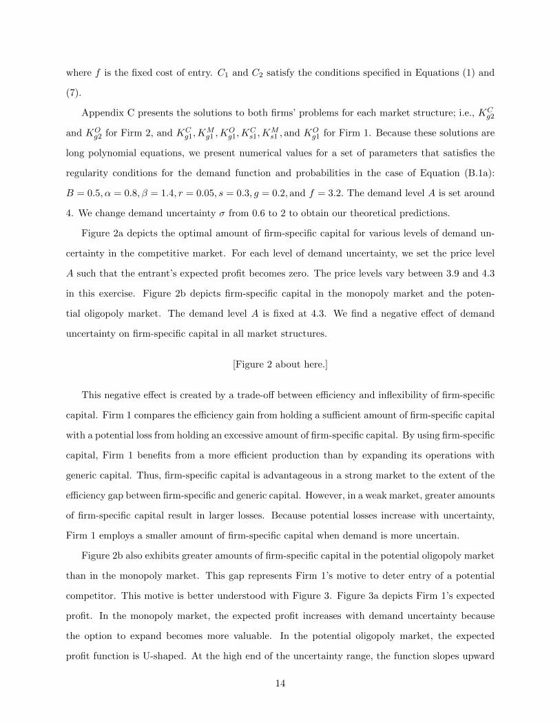
Figure 2a depicts the optimal amount of firm-specific capital for various levels of demand un-

certainty in the competitive market. For each level of demand uncertainty, we set the price level

A such that the entrant’s expected profit becomes zero. The price levels vary between 3.9 and 4.3

in this exercise. Figure 2b depicts firm-specific capital in the monopoly market and the poten-

tial oligopoly market. The demand level A is fixed at 4.3. We find a negative effect of demand

uncertainty on firm-specific capital in all market structures.

[Figure 2 about here.]

This negative effect is created by a trade-off between efficiency and inflexibility of firm-specific

capital. Firm 1 compares the efficiency gain from holding a sufficient amount of firm-specific capital

with a potential loss from holding an excessive amount of firm-specific capital. By using firm-specific

capital, Firm 1 benefits from a more efficient production than by expanding its operations with

generic capital. Thus, firm-specific capital is advantageous in a strong market to the extent of the

efficiency gap between firm-specific and generic capital. However, in a weak market, greater amounts

of firm-specific capital result in larger losses. Because potential losses increase with uncertainty,

Firm 1 employs a smaller amount of firm-specific capital when demand is more uncertain.

Figure 2b also exhibits greater amounts of firm-specific capital in the potential oligopoly market

than in the monopoly market. This gap represents Firm 1’s motive to deter entry of a potential

competitor. This motive is better understood with Figure 3. Figure 3a depicts Firm 1’s expected

profit. In the monopoly market, the expected profit increases with demand uncertainty because

the option to expand becomes more valuable. In the potential oligopoly market, the expected

profit function is U-shaped. At the high end of the uncertainty range, the function slopes upward

14

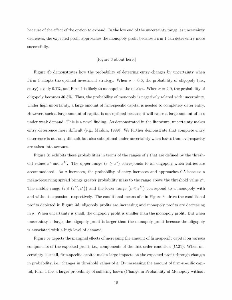
because of the effect of the option to expand. In the low end of the uncertainty range, as uncertainty

decreases, the expected profit approaches the monopoly profit because Firm 1 can deter entry more

successfully.

[Figure 3 about here.]

Figure 3b demonstrates how the probability of deterring entry changes by uncertainty when

Firm 1 adopts the optimal investment strategy. When σ = 0.6, the probability of oligopoly (i.e.,

entry) is only 0.1%, and Firm 1 is likely to monopolize the market. When σ = 2.0, the probability of

oligopoly becomes 36.3%. Thus, the probability of monopoly is negatively related with uncertainty.

Under high uncertainty, a large amount of firm-specific capital is needed to completely deter entry.

However, such a large amount of capital is not optimal because it will cause a large amount of loss

under weak demand. This is a novel finding. As demonstrated in the literature, uncertainty makes

entry deterrence more difficult (e.g., Maskin, 1999). We further demonstrate that complete entry

deterrence is not only difficult but also suboptimal under uncertainty when losses from overcapacity

are taken into account.

Figure 3c exhibits these probabilities in terms of the ranges of ε that are defined by the thresh-

old values ε∗ and εM . The upper range (ε ≥ ε∗) corresponds to an oligopoly when entries are

accommodated. As σ increases, the probability of entry increases and approaches 0.5 because a

mean-preserving spread brings greater probability mass to the range above the threshold value ε∗.

The middle range(ε ∈

(εM , ε∗

))and the lower range

(ε ≤ εM

)correspond to a monopoly with

and without expansion, respectively. The conditional means of ε in Figure 3c drive the conditional

profits depicted in Figure 3d; oligopoly profits are increasing and monopoly profits are decreasing

in σ. When uncertainty is small, the oligopoly profit is smaller than the monopoly profit. But when

uncertainty is large, the oligopoly profit is larger than the monopoly profit because the oligopoly

is associated with a high level of demand.

Figure 3e depicts the marginal effects of increasing the amount of firm-specific capital on various

components of the expected profit; i.e., components of the first order condition (C.21). When un-

certainty is small, firm-specific capital makes large impacts on the expected profit through changes

in probability, i.e., changes in threshold values of ε. By increasing the amount of firm-specific capi-

tal, Firm 1 has a larger probability of suffering losses (Change in Probability of Monopoly without

15

Expansion) and a smaller probability of earning profits (Change in Probability of Monopoly with

Expansion and of Oligopoly). On the other hand, a larger amount of efficient capital increases the

monopoly profit with expansion. Firm 1 chooses the amount of firm-specific capital so that these

effects balance out. When uncertainty is large, altering threshold values produces smaller impacts

on the probabilities. Instead, larger capital investment causes greater losses when demand is weak

(Change in Monopoly Profit without Expansion).

The degree of market concentration can also be plotted against the optimal amount of firm-

specific capital. Figure 4 plots the probability of monopoly, which is a measure of the degree of

market concentration in the model. The figure exhibits a positive relationship between firm-specific

capital and market concentration.

[Figure 4 about here.]

Figures 5 depicts distributions of Firm 1’s realized profits for different values of demand un-

certainty ε based on 5,000 simulations. Figures 5a is for the monopoly market and 5b is for the

potential oligopoly market. Note that the profit in our single-period production model represents

periodic profits as well as the total firm value. When demand uncertainty is small, both distribu-

tions are relatively symmetric and similar to each other. However, when demand uncertainty is

large, then the monopoly profit distribution exhibits positive skewness. This positive skewness is

a result of exercising the expansion option; the firm earns profits from high demand while limiting

losses from weak demand. In contrast, the distribution in the potential oligopoly market is bi-modal

and narrower than in the monopoly case. When demand is high, the second firm enters the market

and eliminates Firm 1’s opportunities to earn high profits. The downward shift of profits forms the

second peak around the value of 3 in profits.

[Figure 5 about here.]

Figure 6 plots relative volatility of profits against relative volatility of demand (σ) for three

market structures. The smallest volatility is normalized to unity. Note that the correlation coef-

ficient between demand shocks and the firm value is one because the demand is the sole source of

uncertainty in this economy. Thus, as Aguerrevere (2009) defines, the elasticity of the firm value

16

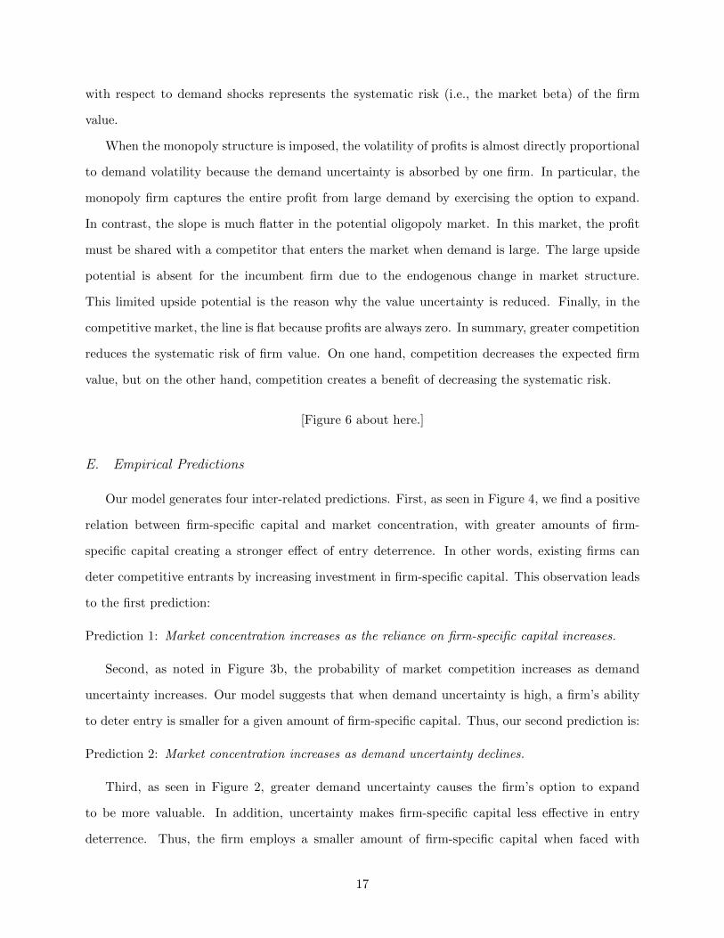
with respect to demand shocks represents the systematic risk (i.e., the market beta) of the firm

value.

When the monopoly structure is imposed, the volatility of profits is almost directly proportional

to demand volatility because the demand uncertainty is absorbed by one firm. In particular, the

monopoly firm captures the entire profit from large demand by exercising the option to expand.

In contrast, the slope is much flatter in the potential oligopoly market. In this market, the profit

must be shared with a competitor that enters the market when demand is large. The large upside

potential is absent for the incumbent firm due to the endogenous change in market structure.

This limited upside potential is the reason why the value uncertainty is reduced. Finally, in the

competitive market, the line is flat because profits are always zero. In summary, greater competition

reduces the systematic risk of firm value. On one hand, competition decreases the expected firm

value, but on the other hand, competition creates a benefit of decreasing the systematic risk.

[Figure 6 about here.]

E. Empirical Predictions

Our model generates four inter-related predictions. First, as seen in Figure 4, we find a positive

relation between firm-specific capital and market concentration, with greater amounts of firm-

specific capital creating a stronger effect of entry deterrence. In other words, existing firms can

deter competitive entrants by increasing investment in firm-specific capital. This observation leads

to the first prediction:

Prediction 1: Market concentration increases as the reliance on firm-specific capital increases.

Second, as noted in Figure 3b, the probability of market competition increases as demand

uncertainty increases. Our model suggests that when demand uncertainty is high, a firm’s ability

to deter entry is smaller for a given amount of firm-specific capital. Thus, our second prediction is:

Prediction 2: Market concentration increases as demand uncertainty declines.

Third, as seen in Figure 2, greater demand uncertainty causes the firm’s option to expand

to be more valuable. In addition, uncertainty makes firm-specific capital less effective in entry

deterrence. Thus, the firm employs a smaller amount of firm-specific capital when faced with

17

greater uncertainty. This observation leads to the third prediction:

Prediction 3: The amount of firm-specific capital utilized by firms is greater when demand uncer-

tainty is smaller.

Finally, from Figure 6, we obtain the last prediction:

Prediction 4: The volatility of firm value is less than directly proportional to the demand volatility

and the slope is steeper in a more concentrated market.

Our predictions concerning the interaction of competition and firm-specific capital were gen-

erated from a stylized two-period model. Thus, in order to empirically test these predictions, we

must adjust the stylized predictions to reflect a multi-period world. For example, the model does

not differentiate between a stock or flow measure of firm-specific capital investment. However, em-

pirically testing the predictions requires that we carefully consider the application of the model to

whether the various predictions apply to a stock or flow measurement of firm-specific investment.

II. Empirical Analysis

In this section, we present the formal empirical analysis of the model’s predictions using a

sample of public firms listed on NYSE, AMEX, and NASDAQ that have balance sheet and income

statement data available on the Compustat annual and quarterly accounting databases and monthly

stock returns reported on the Center for Research in Security Prices (CRSP) database. The sample

comprises firms with two-digit SIC numbers between 01 and 87, excluding real estate investment

trusts (REITs) and other public real estate firms, hotels and lodging, and investment holding

companies.

We restrict our analysis to firms with information recorded in the Compustat dataset over the

period 1984 to 2012 that have positive total assets (TA), property, plant and equipment (PPE),

net sales (Sales), and real estate data reported on the balance sheet.16 Our final sample consists of

11,708 firms belonging to 65 two-digit SIC code industries. Table I shows the frequency distribution

of firms and industries over the sample period. The sample contains an average of 3,993 firms per

year, ranging from 2,874 firms in 2012 to 5,627 firms in 1997.

In the theoretical model, we characterize firm-specific capital as (1) taking time to build, (2)

18

being fixed in size, (3) determining the production capacity, and (4) improving operational efficiency.

Thus, in order to test the model’s predictions we use owned corporate real estate as a proxy

for firm-specific capital. Corporate real estate assets include factories, warehouses, offices, and

retail facilities. Investing in real estate requires a significant amount of time. Real estate largely

determines production capacity, and it is difficult to adjust its size once developed. Owned real

estate that is tailored for a firm improves production efficiency (e.g., a factory designed for a

particular production process). We also consider long-term leased real estate as equivalent to

owned real estate (e.g., a single-tenant warehouse that is designed specifically for the tenant firm).

By contrast, short-term rental spaces are considered to be generic capital.

We construct the firm-specific capital measure using the Compustat PPE account, which in-

cludes buildings, machinery and equipment, capitalized leases, land and improvements, construc-

tion in progress, natural resources, and other assets. Following the literature, we measure firm-

specific capital by adding buildings, land and improvements, and construction in progress in PPE

(RE Asset1 ). Then we construct a normalized measure of firm-specific capital STC1 by taking

its ratio to PPE. For the empirical analysis that follows, we use STC1 as the primary measure of

firm-specific capital.17

We measure industry concentration using the Herfindahl-Hirschman Index (HHI) computed on

the basis of net sales.18 Again, industry classifications are based on two-digit SICs, with industry

concentrations computed every year using the annual net sales from Compustat.19

In the theoretical model, the industry-wide demand shock is the sole source of uncertainty and

affects the revenue and profits of both the incumbent firm and the entrants. To construct a proxy for

the demand uncertainty, we use the year-on-year quarterly net sales growth from the Compustat

data series. The sales growth is primarily driven by demand shocks rather than supply shocks

because a demand shock changes price and quantity in the same direction whereas a supply shock

changes price and quantity in the opposite directions. We first compute the time-series variance of

the industry mean quarterly sales growth rate. The variance is measured on a rolling basis using 20

and 40-quarter look-back windows. Because this variance measure is biased due to the time-varying

number of observations in an industry, we make a statistical adjustment as detailed in Appendix D

to remove the effect of the number of observations. We use the standard deviation as the volatility

measure.

19

The realized volatility at the time of production is suitable for studying the effect of volatility on

HHI because the contemporaneous level of uncertainty affects firms’ entry decisions. However, this

realized measure is not the best to study the effect of volatility on corporate investments because

firms make their investment decisions on the basis of forecasts of the future demand uncertainty

that will affect their production. In the theoretical model, this timing gap is not an issue because

the demand uncertainty is constant over time. In our empirical analysis, we mimic firms’ forecasts

of the industry sales volatility by estimating an ARIMA(1,1,0) model on a 20-quarter rolling basis.20

In addition, we compute the volatility of firm value to test Prediction 4. Because the theoretical

model is a two-period model, firms’ profits are equivalent to the firm value. In the empirical test,

periodic profits are not a good measure because profit growth is highly correlated with sales growth,

which we use for demand uncertainty. Moreover, the gap between sales volatility and profit volatility

is primarily determined by the operating leverage (i.e., the amount of fixed costs in production).

Thus, we use the variance of quarterly changes in firm value based on the monthly CRSP data

series.

A. Descriptive Statistics

Table II presents the industry level descriptive statistics for the 29-year period from 1984 to 2012.

The average industry contains 69 firms and has an HHI of 0.19 - the corresponding median values

are 27 firms and an HHI of 0.14. The average level of concentration among the 65 industries varies

considerably from 0.02, which is characteristic of a very competitive industry, to 0.83, indicating a

highly concentrated industry - we impose a cutoff of three firms minimum per industry. The most

competitive industry in our sample consists of 534 firms.

Also, average firm size (whether measured by market value, sales, or total assets in 2012 U.S.

dollars) increases with industry concentration. The distribution of firm sizes in our sample is

positively skewed with a mean and a median total assets per firm of $615 million and $64 million,

respectively. Understandably, our sample is dominated by relatively small firms mostly operating

in competitive industries. As expected, leverage and industry concentration are also positively

related for good reasons. As noted in the introduction, the average amount of firm-specific capital

owned by firms in our sample is 27% of PPE. The average annual rent expense for our sample is

roughly $2.3 million, which capitalized at a reasonable rate of return to estimate the value of the

20

associated real estate space, indicates a relatively small use of generic capital assets as compared

to the average stock of firm-specific capital assets owned by these firms.

The bottom section of Table II presents the summary statistics of our measures of sales volatility

and firm value volatility computed on the rolling 20- and 40-quarter basis. The adjusted variance

of sales growth sometimes exhibits negative values because of the adjustment outlined in Appendix

D. However, this does not affect our results because the relative volatilities are what matters.

B. Results

B.1. Predictions 1 and 2

Prediction 1 concerns a causal relationship that the use of firm-specific capital increases industry

concentration (the entry deterrence effect). Prediction 2 indicates that demand uncertainty is a

confounding factor for the causal relationship because demand uncertainty negatively affects both

industry concentration and the investment in firm-specific capital. To test these predictions, we

estimate via ordinary least squares (OLS) the following panel regression model with year fixed

effects:

HHIit = α+ β × STC1it + γ × V OLit + yt + εit. (25)

where HHIit is the Herfindahl-Hirschman Index for industry i in year t and represents our proxy for

market concentration; STC1it represents our proxy for firm-specific capital; and V OLit represents

our proxy for the industry demand uncertainty.21

Firm-specific capital determines the production capacity and thus, the current level of firm-

specific capital is our primary measure. However, it can take several years until we observe the

effect of firm-specific capital on market concentration. To estimate the effect of past values of

firm-specific capital, we also estimate Equation (25) by decomposing STC1it into STC1i,t−3 +

∆STC1i,t−2 + ∆STC1i,t−1 + ∆STC1i,t, where ∆STC1i,t represents the change in firm-specific

capital between t − 1 and t. Thus, the β coefficient on the single current variable equals the

weighted average of the coefficients on the decomposed terms.

Regarding the demand uncertainty, the current level is also our primary measure because the

entry decision of a competitor is based on the current level of demand uncertainty. However,

previous forecasts may affect the market concentration if the entry decision was made several years

21

before production on the basis of volatility forecasts. Thus, we also include the 1, 2, and 3-year

forecast errors of our ARIMA(1,1,0) model.

Table III reports the results, all of which are consistent with the predictions. When only

STC1it is included (column 1), the estimated coefficient is 0.20 and statistically significant at

the 1% level. When STC1it is decomposed (column 2), we see that firm-specific capital that

was in place 3-years before production makes the largest impact on market concentration (0.25).

The impact monotonically decreases as the timing of investment becomes closer to production.

However, all coefficients are positive and statistically significant at least at the 5% level. Thus,

market concentration increases with several years of lags as the reliance on firm-specific capital

increases.

[Table III about here.]

Columns 3 and 4 report the test results on Prediction 2 when the 20-quarter rolling volatility

measure is used. The 40-quarter rolling volatility gives consistent results. The estimated coefficient

on the current sales volatility is −0.28 and −0.22 for specifications with and without past forecast

errors, respectively. These coefficients are both statistically significant at the 1% level but coeffi-

cients on the past forecast errors are not statistically significant. Thus, the demand volatility at

the time of production negatively affects market concentration.

These results are robust when we include both firm-specific capital and demand uncertainty

(columns 5 and 6): Market concentration is positively affected by firm-specific capital, especially by

the 3-year old stock, after controlling for the negative effect of demand uncertainty. These results

strongly support Predictions 1 and 2. The coefficients imply that, on average, a one standard

deviation increase in firm-specific capital (from 27% to 39%) increases the average HHI by 0.024

points (from 0.187 to 0.211). A one standard deviation increase in demand uncertainty (from 3.9

% to 13.9%) decreases the average HHI by 0.033 points (from 0.187 to 0.154).

In addition to the average relation, we also investigate the temporal variation in the effect of

firm-specific capital by estimating the following regression that allows for time-varying betas:

HHIit = α+ βt × STC1it + yt + εit. (26)

22

Figure 7 plots the yearly estimated coefficients. We note that in all years, we obtain a positive

coefficient, which is consistent with Prediction 1. Although cycles are observed, the year-specific

coefficient appears stationary. Interestingly, the coefficient is larger during the recession periods of

the early 1990’s, the early 2000’s, and the late 2000’s.

[Figure 7 about here.]

Similarly, for Prediction 2, we estimate the following model with time-varying beta:

HHIit = α+ βt × V OLit + yt + εit. (27)

Figure 8 plots the yearly estimated coefficients. The estimated coefficient is negative for 26 years

during the 36-year sample period when we use 20-quarter volatility. The coefficient is negative for

25 years during the 32-year period when we use 40-quarter volatility. The mean coefficient is −0.23

and −0.30 for the 20- and 40-quarter measures, respectively. These mean values are consistent with

the estimated coefficient from the constant-coefficient model.

[Figure 8 about here.]

B.2. Prediction 3

We now turn to the model’s prediction concerning the negative relation between the investment

in firm-specific capital and demand uncertainty. We note the timing gap between the initial in-

vestment and the demand uncertainty in the production phase. Thus, we use the ARIMA(1,1,0)

volatility forecasts in the following panel regression model with year fixed effects:

STC1it = α+ β × Et [V OLi,t+q] + yt + εit, (28)

where Et [V OLi,t+q] is the q-quarter ahead forecast of industry i’s level of sales volatility. We

compute the 20- and 40-quarter rolling volatility measures adjusted for the time-varying sample

size as described in Appendix D. Then we construct the 4, 8, and 12-quarter ahead forecasts.

Table IV reports the estimation result. Consistent with the theoretical prediction, the estimated

coefficients are negative and statistically significant at the 10% level or higher in all specifications.

23

For the 40-quarter rolling volatility measure (columns 4, 5, and 6), the estimated coefficients are

−0.0956, −0.0677, and −0.0481 when 4-, 8-, and 12-quarter ahead forecasts are used, respectively.

The effect of uncertainty is strongest when the 4-quarter forecasting horizon is used. Thus, firms

employ a smaller amount of firm-specific capital if they expect greater demand uncertainty for the

next year. The effects are economically significant because a one percentage point change in the

ratio requires a large change in capital investment that increases the total PPE by more than one

percent after depreciation.

[Table IV about here.]

In addition to the average impact of demand uncertainty on the use of firm-specific capital, we

also investigate the time variation in the parameter coefficient by estimating the following regression

that allows for time-varying betas:

STC1it = α+ βt × Et [V OLi,t+q] + yt + εit. (29)

Figure 9 depicts the estimation result using the 8-quarter ahead forecasts of demand volatility.22

The estimated coefficient is negative for 17 years in the 29-year period when we use 20-quarter

volatility, and for 19 years in the 27-year period when we use 40-quarter volatility. Interestingly,

the coefficients are positive during recessions in the early 1990’s and early and late 2000’s especially

when 20-quarter rolling volatility is used.

[Figure 9 about here.]

B.3. Prediction 4

Table V reports the result of the OLS estimation of panel regression model:

V OLvalueit = α1 + (β1 + β2HHIit)V OLsalesit + LDt{α2 + (β3 + β4HHIit)V OL

salesit }+ εit, (30)

where V OLvalueit is industry i’s firm value volatility at time t and LDt is a dummy variable that

represents the low demand state. We use three measures of LDt: the NBER recession periods,

periods of low growth in aggregate sales, and periods of low growth in individual industry sales.

24

Our model predicts that the coefficient β1 is positive and smaller than one and β2 is positive. In

addition we test Aguerrevere’s (2009) predictions that β4 and β2 +β4 are negative and that β1 +β3

and β1 + β2 + β3 + β4 are positive.

[Table V about here.]

Columns (1) and (2) report the results when we impose α2 = β3 = β4 = 0. When β2 = 0

is further imposed (column (1)), the estimated value of β1 is 0.31, which represents the average

slope for various concentration levels in both demand states. This estimate is consistent with

our model’s prediction. When the restriction on β2 is relaxed in column (2), the coefficient on

the interaction term is positive and statistically significant. The estimated slopes are 0.13 for

a perfectly competitive market (β2) and 0.78 for a monopoly market (β1 + β2). The estimated

coefficients confirm that the firm value risk is greater in a more concentrated market.

In columns (3), (4), and (5), we report the results when we condition on the low demand state.

The main effects of β1 and β2 are positive and statistically significant at the 1 % level. The estimate

for β4 is positive when the NBER period is used, but is negative when low sales growth measures

are used. In particular, the coefficient is statistically significant when we use the aggregate sales

growth. Although this negative coefficient is consistent with Aguerrevere’s (2009) model, the sum

of β2 and β4 is still positive. Thus, we find that the firm value is riskier in a more concentrated

market regardless of demand levels. One possible explanation for this result is that the U.S. market

since 1984 has been in a sufficiently high demand state where the option to expand has a large

value.

III. Conclusion

This study provides a better understanding for why firms own firm-specific capital as opposed

to leasing more generic capital. We also investigate how the market structure and the firm value

risk are endogenously determined by firm-specific investments. We build a model that captures

realistic features of corporate investments to study the interaction between firm-specific capital

and product market competition under uncertainty. In our model, firms choose investment in firm-

specific capital after taking into account its effect on the product market competition and thus on

25

the firm value. Our four predictions and strong empirical support reveal important interactions

among demand uncertainty, firm-specific capital, market competition, and the systematic risk of

firms.

The key insights from our analysis are that market competition is negatively related to the

use of firm-specific capital investment due to its entry deterrence effect. However, our analysis

shows that demand uncertainty increases the costs associated with firm-specific investments creating

opportunities for entrants. Our empirical findings support the causal entry deterrence effect of firm-

specific capital after controlling for the confounding effect of demand volatility. Our second key

insight is that market competition results in lower firm risk.

Our findings have implications on anti-trust policies. Our model predictions show that a pos-

itive relation between uncertainty and competition implies that a current risky economic environ-

ment naturally enhances market competition. Moreover, the positive relation between firm-specific

capital investments and market concentration implies that anti-trust policies may have unwanted

consequences on investments in various forms of firm-specific capital such as real estate, equipment,

R&D, and employee training. As a result, recent Department of Justice antitrust actions in the

telecommunications and pharmaceutical industries could result in significantly lower future research

and development spending.

26

References

Aguerrevere, Felipe L., 2003, Equilibrium investment strategies and output price behavior: A real-

options approach, Review of Financial Studies 16, 1239–1272.

, 2009, Real options, product market competition, and asset returns, The Journal of Finance

64, 957–983.

Allen, Beth, 1993, Capacity precommitment as an entry barrier for price-setting firms, International

Journal of Industrial Organization 11, 63 – 72.

, Raymond Deneckere, Tom Faith, and Dan Kovenock, 2000, Capacity precommitment as

a barrier to entry: A bertrand-edgeworth approach, Economic Theory 15, 501–530.

Bain, Joe S., 1954, Economies of scale, concentration, and the condition of entry in twenty manu-

facturing industries, The American Economic Review 44, 15–39.

Basu, Kaushik, and Nirvikar Singh, 1990, Entry-deterrence in stackelberg perfect equilibria, Inter-

national Economic Review 31, pp. 61–71.

Berk, Jonathan B., Richard C. Green, and Vasant Naik, 1999, Optimal investment, growth options,

and security returns, The Journal of Finance 54, 1553–1607.

Brander, James A., and Tracy R. Lewis, 1986, Oligopoly and financial structure: The limited

liability effect, The American Economic Review 76, 956–970.

Bulow, Jeremy, John Geanakoplos, and Paul Klemperer, 1985, Holding idle capacity to deter entry,

The Economic Journal 95, 178–182.

Carlson, Murray, Adlai Fisher, and Ron Giammarino, 2004, Corporate investment and asset price

dynamics: Implications for the cross-section of returns, The Journal of Finance 59, 2577–2603.

Caves, R. E., and M. E. Porter, 1977, From entry barriers to mobility barriers: Conjectural decisions

and contrived deterrence to new competition, The Quarterly Journal of Economics 91, 241–262.

Chevalier, Judith A., 1995, Do lbo supermarkets charge more? an empirical analysis of the effects

of lbos on supermarket pricing, The Journal of Finance 50, 1095–1112.

27

Cooper, Ilan, 2006, Asset pricing implications of nonconvex adjustment costs and irreversibility of

investment, The Journal of Finance 61, 139–170.

Dixit, Avinash, 1979, A Model of Duopoly Suggesting a Theory of Entry Barriers, Bell Journal of

Economics 10, 20–32.

, 1980, The role of investment in entry-deterrence, The Economic Journal 90, 95–106.

Dixit, Avinash K, and Robert S Pindyck, 1994, Investment under uncertainty (Princeton University

Press).

Eaton, B. Curtis, and Richard G. Lipsey, 1980, Exit barriers are entry barriers: The durability of

capital as a barrier to entry, The Bell Journal of Economics 11, 721–729.

Ellison, Glenn, and Sara Fisher Ellison, 2011, Strategic entry deterrence and the behavior of phar-

maceutical incumbents prior to patent expiration, American Economic Journal: Microeconomics

3, 1–36.

Fama, Eugene F, and Merton H Miller, 1972, The Theory of Finance (Dryden Press, Hinsdale, IL).

Fresard, Laurent, 2010, Financial strength and product market behavior: The real effects of cor-

porate cash holdings, The Journal of Finance 65, 1097–1122.

Gersbach, Hans, and Armin Schmutzler, 2012, Product markets and industry-specific training, The

RAND Journal of Economics 43, 475–491.

Glazer, Jacob, 1994, The strategic effects of long-term debt in imperfect competition, Journal of

Economic Theory 62, 428 – 443.

He, Hua, and Robert S. Pindyck, 1992, Investments in flexible production capacity, Journal of

Economic Dynamics and Control 16, 575 – 599.

Hoberg, Gerard, Gordon Phillips, and Nagpurnanand Prabhala, 2014, Product market threats,

payouts, and financial flexibility, The Journal of Finance 69, 293–324.

Igami, Mitsuru, and Nathan Yang, 2014, Cannibalization and preemptive entry in heterogeneous

markets, SSRN Working Paper 2271803.

28

Kovenock, Dan, and Gordon Phillips, 1995, Capital structure and product-market rivalry: How do

we reconcile theory and evidence?, The American Economic Review 85, 403–408.

Leary, Mark T, and Michael R Roberts, 2014, Do peer firms affect corporate financial policy?, The

Journal of Finance 69, 139–178.

Lyandres, Evgeny, 2006, Capital structure and interaction among firms in output markets: Theory

and evidence, The Journal of Business 79, 2381–2421.

MacKay, Peter, and Gordon M. Phillips, 2005, How does industry affect firm financial structure?,

Review of Financial Studies 18, 1433–1466.

Maksimovic, Vojislav, 1988, Capital structure in repeated oligopolies, The RAND Journal of Eco-

nomics 19, 389–407.

Maskin, Eric S., 1999, Uncertainty and entry deterrence, Economic Theory 14, pp. 429–437.

Pindyck, Robert S., 1988, Irreversible investment, capacity choice, and the value of the firm, The

American Economic Review 78, pp. 969–985.

Smiley, Robert, 1988, Empirical evidence on strategic entry deterrence, International Journal of

Industrial Organization 6, 167 – 180.

Spence, A. Michael, 1977, Entry, capacity, investment and oligopolistic pricing, The Bell Journal

of Economics 8, 534–544.

Spulber, Daniel F., 1981, Capacity, output, and sequential entry, The American Economic Review

71, 503–514.

Wenders, John T., 1971, Excess capacity as a barrier to entry, The Journal of Industrial Economics

20, 14–19.

29

Notes

1See Fama and Miller (1972) and the references therein for a complete discussion of the devel-

opment of the ‘market value rule’ governing management decision making.

2Although our model is predicated on the observation that capital investments can be firm-

specific or generic, Gersbach and Schmutzler (2012) derive a model that allows for strategic in-

vestments in labor that produces similar insights. In their model, labor expenses associated with

training serves as a firm-specific investment that affects the firm’s product market by deterring

potential competitors from entering the market.

3Estimates are that over 500 automobile manufacturers entered the U.S. market between 1902

and 1910. (Source: “The Automobile Industry, 1900-1909” accessed on June 1, 2014 at http:

//web.bryant.edu/~ehu/h364/materials/cars/cars_10.htm)

4Source: “History of the Rouge” accessed on June 1, 2014 at http://www.thehenryford.org/

rouge/historyofrouge.aspx

5See Igami and Yang (2014).

6http://www.businessweek.com/articles/2013-04-04/apples-campus-2-shapes-up-as-an-

investor-relations-nightmare

7Both models introduce an option to expand, but Aguerrevere considers a repeated Cournot

competition among existing firms and we consider a Stackelberg-type competition between an

incumbent and new entrants.

8The capital in the model obviously includes but is not limited to real estate. For example,

human capital and research and development may also be considered as firm-specific capital.

9Source: http://www.federalreserve.gov/releases/z1/20110310/

10Dixit and Pindyck (1994) note that real estate investments may provide firms with options to

grow production.

11This is the simplest form of multi-period models to analyze long-term commitments. Extending

the production period will not change our result.

12Thus, for ease of exposition we refer to the firm in the monopoly case as Firm 1 to note that

it is the first firm to enter the market.

13This option to expand is a deviation from the Stackelberg model.

30

14He and Pindyck (1992) make the same assumption about the cost associated to generic capital

since it can interchangeably be used to produce either of two products whereas firm-specific capital

is product-specific in their model.

15Technically, the Leibniz integral rule is applied to conditional expectations to derive partial

derivatives of the expected profit with respect to firm-specific capital.

16Prior to 1984, PPE accounts were reported net of depreciations. Compustat switched to a

cost basis reporting with accrued depreciation contra accounts from 1984 onward. For consistency

purposes, we restrict our analyze to this period. However, reported tests based on the 40-year

period from 1973 to 2012 show similar results.

17We could also use capital investment as a measure of firm-specific capital because, in the

theoretical model, capital investment is equivalent to the stock of capital. Our current stock

measure is relevant as a proxy for capacity.

18The HHI of an industry is the sum of the squares of the individual firms’ net sales to total

industry net sales. The higher the number of firms in an industry is, the smaller the resulting

industry’s HHI will be. The HHI is based on net sale because gross sales figures are not available

on Compustat. Our industry concentration measure does not account the effect of imports from

non-US listed firms. But since it omits exports by US firms, the net effect should be smaller.

19We also present industry concentrations based on total assets in Table (2).

20The positive autocorrelations of our volatility measure almost completely disappear when we

take the first difference. Thus, we estimate a simple AR(1) model for volatility changes.

21HHIit is bounded between 0 and 1, with monopoly industries having a value of 1 and perfectly

competitive industries having a value of 0. STC1it is also bounded between 0 and 1 because it is

the ratio to total PPE.

22The results with other forecast horizons are almost identical.

31

Appendix A Proof of Proposition 1

Without loss of generality, consider the 2-firm Cournot equilibrium represented by Equations

(13) and (14). When ε = ε∗, Firm 2’s profit is zero:

Π2 = P(Ks1,K

Eg1 (Ks1, ε

∗) ,KEg2 (Ks1, ε

∗) , ε∗)×Kg2 − C2

(KEg2 (Ks1, ε

∗))

= 0 (A.1)

We rewrite Equation (A.1) by using Firm 2’s FOC:

Π2 =−∂P(Ks1,K

Eg1 (Ks1, ε

∗) ,KEg2 (Ks1, ε

∗) , ε∗)

∂KEg2

× KEg2

2(Ks1, ε

∗)

+ C ′2(KEg2 (Ks1, ε

∗))×Kg2 (Ks1, ε

∗)− C2

(KEg2 (Ks1, ε

∗))

= 0 (A.2)

By totally differentiating Equation (A.2), we obtain

− ∂2P

∂KEg2

2 KEg2

2 ×

(dKs1 +

∂KEg1

∂Ks1dKs1 +

∂KEg1

∂ε∗dε∗ +

∂KEg2

∂Ks1dKs1 +

∂KEg2

∂ε∗dε∗ + dε∗

)

− 2∂P

∂KEg2

KEg2 ×

(∂KE

g2

∂Ks1dKs1 +

∂KEg2

∂ε∗dε∗

)+ C ′′2K

Eg2 ×

(∂KE

g2

∂Ks1dKs1 +

∂KEg2

∂ε∗dε∗

)

+ C ′2 ×

(∂KE

g2

∂Ks1dKs1 +

∂KEg2

∂ε∗dε∗

)− C ′2 ×

(∂KE

g2

∂Ks1dKs1 +

∂KEg2

∂ε∗dε∗

)= 0. (A.3)

By assuming an affine demand function, the first term is eliminated (∂2P/∂KE

g22

= 0). The last

two terms cancel out. By rearranging the equation, we obtain:

dε∗

dKs1= −

(∂KE

g2

∂ε

∗)−1(∂KE

g2

∂Ks1

). (A.4)

Since Firm 2 chooses a larger amount of capital for a greater demand and a smaller amount of Firm

1’s firm-specific capital, ∂KEg2

/∂ε∗ > 0 and ∂KE

g2

/∂Ks1 < 0. As a result, we derive Equation (15)

in Proposition 1:

dε∗

dKs1> 0. (A.5)

�

32

Appendix B Variations in Firm 1’s problem under potential

oligopoly

Variation 1: If εM < εE < ε∗,

maxKs1

E [Π1(Ks1,Kg1,Kg2, ε)]

≡ E[ΠO

1 (Ks1,KEg1,K

Eg2, ε) |ε ≥ ε∗(Ks1)

]Pr (ε ≥ ε∗(Ks1))

+ E[ΠM

1 (Ks1,KMg1 , ε)

∣∣ε∗(Ks1) > ε > εM (Ks1)]Pr(ε∗(Ks1) > ε > εM (Ks1)

)+ E

[ΠM

1 (Ks1, 0, ε)∣∣ε ≤ εM (Ks1)

]Pr(ε ≤ εM (Ks1)

). (B.1a)

Variation 2: If εM < ε∗ < εE ,Equation (16)

Variation 3: If ε∗ < εM < εE ,

maxKs1

E [Π1(Ks1,Kg1,Kg2, ε)]

≡ E[ΠO

1 (Ks1,KEg1,K

Eg2, ε)

∣∣ε > εE(Ks1)]Pr(ε > εE(Ks1)

)+ E

[ΠO

1 (Ks1, 0,KEg2, ε)

∣∣ε∗(Ks1) ≤ ε ≤ εE(Ks1)]Pr(ε∗(Ks1) ≤ ε ≤ εE(Ks1)

)+ E

[ΠM

1 (Ks1, 0, ε) |ε < ε∗(Ks1)]Pr (ε < ε∗(Ks1)) , (B.1b)

33

Appendix C Solution of the model

A Firms’ Decision for the second period

A.1 Firm 1

At t1, Firm 1 solves the problem specified in Equation (3), taking Ks1, Kg2, and ε̄ as given.

Since the objective function is quadratic, SOC is readily satisfied. From FOC and the sign condition

on Kg1, the optimal choice of Kg1 is:23

Monopoly:KMg1 =

A− g − (2B + α)Ks1 + ε̄

2B + βif ε̄ > g −A+ (2B + α)Ks1 ≡ εM

0 otherwise.

(C.1)

Oligopoly:KOg1 =

A− g − (2B + α)Ks1 −BKg2 + ε̄

2B + βif ε̄ > g −A+ (2B + α)Ks1 +BKg2 ≡ εO

0 otherwise.

(C.2)

Competitive:KCg1 =

A− g + ε̄− αKs1

βif ε̄ > g −A+ αKs1 ≡ εC

0 otherwise.

(C.3)

A.2 Firm 2

At t1, Firm 2 solves the problem specified in Equation (9), taking Ks1, Kg1, and ε̄ as given. Since

the objective function is quadratic, SOC is readily satisfied. From FOC and the entry condition

34

(10), the optimal choice of Kg2 is

Oligopoly:KOg2 =

A− g −B(Ks1 +Kg1) + ε̄

2B + β

if ε̄ ≥ g −A+B(Ks1 +Kg1)

+√

2(2B + β)(1 + r)f

0 otherwise.

(C.4)

Competitive:KCg2 =

A− g + ε̄

βif ε̄ ≥ g −A+

√2β(1 + r)f

0 otherwise.

(C.5)

B Cournot Nash Equilibrium in the second period

When both firms employ positive amounts of generic capital, the Cournot Nash equilibrium

levels of generic capital, Equations (13) and (14), are expressed as:24

KEg1 = L− (1−M)Ks1, (C.6)

KEg2 = L−NKs1, (C.7)

where

L ≡ A− g + ε̄

3B + β> 0,

M ≡ (β − α)(2B + β)

(3B + β)(B + β)∈ (0, 1)

N ≡ B(β − α)

(3B + β)(B + β)> 0.

Firm 2’s entry condition (10) gives the threshold value of demand shock ε∗:

ε∗(Ks1) ≡ g −A+

√2(3B + β)2(1 + r)f

2B + β+B(β − α)

B + βKs1. (C.8)

We confirm the entry deterrence effect (15); i.e., a larger firm-specific capital of Firm 1 makes it

less unlikely for Firm 2 to enter the market. We can also rewrite Firm 1’s expansion condition

35

(C.2) for this Cournot equilibrium:

ε̄ > g −A+

(3B + β − (β − α)(2B + β)

B + β

)Ks1 ≡ εE(Ks1). (C.9)

C Initial choice of firm-specific capital

At t0, Firm 1 solves the problems specified in Equations (5), (16), and (20). In this appendix,

we solve for the optimal choice of firm-specific capital for each market structure.

C.1 Monopoly Market

In the monopoly market, Firm 1’s problem is:

maxKs1

E[ΠM

1 (Ks1,Kg1, ε)]

= E[ΠM

1 (Ks1,KMg1 , ε)

∣∣ε̄ > εM (Ks1)]Pr(ε̄ > εM (Ks1))

+ E[ΠM

1 (Ks1, 0, ε)∣∣ε̄ ≤ εM (Ks1)

]Pr(ε̄ ≤ εM (Ks1)), (C.10a)

ΠM1 (Ks1, 0, ε) = −(1 + r)2f + εKs1 + (A− s)Ks1 −

(B +

α

2

)K2s1, (C.10b)

ΠM1 (Ks1,K

Mg1 , ε) = RM + SMε2 + TMε+ UMεKs1 + VMKs1 +WMK2

s1, (C.10c)

RM ≡ −(1 + r)2f +(A− g)2

2(2B + β), (C.10d)

SM ≡ 1

2(2B + β), (C.10e)

TM ≡ A− g2B + β

, (C.10f)

UM ≡ β − α2B + β

(C.10g)

VM ≡ A(β − α) + g(2B + α)

2B + β− s, (C.10h)

WM ≡ −α2− B(β − α)2

(2B + β)2+α(2B + α)

2B + β− β(2B + α)2

2(2B + β)2. (C.10i)

36

The first-order condition is:

dE[ΠM

1 (Ks1,Kg1, ε)]

dKs1

=dE[ΠM

1 (Ks1,KMg1 , ε)

∣∣ε̄ > εM (Ks1)]

dKs1× Pr

(ε̄ > εM (Ks1)

)+ E

[ΠM

1 (Ks1,KMg1 , ε)

∣∣ε̄ > εM (Ks1)]×dPr

(ε̄ > εM (Ks1)

)dKs1

+dE[ΠM

1 (Ks1, 0, ε)∣∣ε̄ ≤ εM (Ks1)

]dKs1

× Pr(ε̄ ≤ εM (Ks1)

)+ E

[ΠM

1 (Ks1, 0, ε)∣∣ε̄ ≤ εM (Ks1)

]×dPr

(ε̄ ≤ εM (Ks1)

)dKs1

= 0. (C.11)

The specific expression for each of eight elements is as follows.

Pr(ε̄ > εM (Ks1)

)=

√3σ − εM

2√

3σ=

1

2+A− g2√

3σ− 2B + α

2√

3σKs1, (C.12)

dPr(ε̄ > εM (Ks1)

)dKs1

= −2B + α

2√

3σ, (C.13)

Pr(ε̄ ≤ εM (Ks1)

)=

1

2+−A+ g

2√

3σ+

2B + α

2√

3σKs1, (C.14)

dPr(ε̄ ≤ εM (Ks1)

)dKs1

=2B + α

2√

3σ, (C.15)

E[ΠM

1 (Ks1,KMg1 , ε)

∣∣ε̄ > εM (Ks1)]

=

∫ √3σεM (Ks1)

(RM + SMε2 + TMε+ UMεKs1 + VMKs1 +WMK2

s1

) 1

2√

3σdε̄

=

(RM + VMKs1 +WMK2

s1

) (√3σ − εM

)2√

3σ+

(TM + UMKs1

) (3σ2 − εM

2)

4√

3σ

+SM

(3√

3σ3 − εM3)

6√

3σ, (C.16)

E[ΠM

1 (Ks1, 0, ε)∣∣ε̄ ≤ εM (Ks1)

]=

∫ εM (Ks1)

−√3σ

(−(1 + r)2f + εKs1 + (A− s)Ks1 −

(B +

α

2

)K2s1

) 1

2√

3σdε̄

=

[−(1 + r)2f + (A− s)Ks1 −

(B + α

2

)K2s1

] (εM +

√3σ)

2√

3σ+Ks1

(εM

2 − 3σ2)

4√

3σ. (C.17)

37

By using Leibniz rule of integration,

dE[ΠM

1 (Ks1,KMg1 , ε)

∣∣ε̄ > εM (Ks1)]

dKs1

=

(VM + 2WMKs1

) (√3σ − εM

)2√

3σ+UM

(3σ2 − εM

2)

4√

3σ

− (2B + α)

2√

3σ

(RM + SM εM

2+ TMεM + UMεMKs1 + VMKs1 +WMK2

s1

), (C.18)

dE[ΠM

1 (Ks1, 0, ε)∣∣ε̄ ≤ εM (Ks1)

]dKs1

=[A− s− (2B + α)Ks1]

(εM +

√3σ)

2√

3σ+εM

2 − 3σ2

4√

3σ

+(2B + α)

2√

3σ

[−(1 + r)2f + εMKs1 + (A− s)Ks1 −

(B +

α

2

)K2s1

]. (C.19)

The first order condition (C.11) is a cubic function of Ks1. The solution needs to satisfy non-

negativity conditions on quantity and price and regularity conditions on probabilities. The existence

and uniqueness of the solution depends on specific parameter values. In our numerical exercise, a

unique solution exists after applying regularity conditions.

38

C.2 Potential Oligopoly Market

In our numerical analysis, we focus on the first variation (εM < εE < ε∗, ) of Firm 1’s problem

(B.1a) as a reasonable case:

maxKs1

E[ΠO

1 (Ks1,Kg1,Kg2, ε)]

≡ E[ΠO

1 (Ks1,KEg1,K

Eg2, ε) |ε ≥ ε∗(Ks1)

]Pr (ε ≥ ε∗(Ks1))

+ E[ΠM

1 (Ks1,KMg1 , ε)

∣∣ε∗(Ks1) > ε > εM (Ks1)]

(C.20a)

× Pr(ε∗(Ks1) > ε > εM (Ks1)

)+ E

[ΠM

1 (Ks1, 0, ε)∣∣ε ≤ εM (Ks1)

]Pr(ε ≤ εM (Ks1)

), (C.20b)

ΠO1 (Ks1,K

Eg1,K

Eg2, ε) = RO + SOε2 + TOε+ UOεKs1 + V OKs1 +WOK2

s1, (C.20c)

RO ≡ −(1 + r)2f +(A− g)2(2B + β)

2(3B + β)2, (C.20d)

SO ≡ 2B + β

2(3B + β)2, (C.20e)

TO ≡ (A− g)(2B + β)

(3B + β)2, (C.20f)

UO ≡ BN + β − α3B + β

(C.20g)

V O ≡ g − s+(A− g)(BN + β − α)

3B + β, (C.20h)

WO ≡ BMN + (β − α)(M − 1

2)− M2

2(2B + β). (C.20i)

39

The first-order condition is:

dE[ΠO

1 (Ks1,KEg1,K

Eg2, ε)

]dKs1

=dE[ΠO

1 (Ks1,KEg1,K

Eg2, ε) |ε̄ ≥ ε∗(Ks1)

]dKs1

× Pr (ε̄ ≥ ε∗(Ks1))

+ E[ΠO

1 (Ks1,KEg1,K

Eg2, ε) |ε̄ ≥ ε∗(Ks1)

]× dPr (ε̄ ≥ ε∗(Ks1))

dKs1

+dE[ΠM

1 (Ks1,KMg1 , ε)

∣∣εM (Ks1) < ε̄ < ε∗(Ks1)]

dKs1× Pr

(εM (Ks1) < ε̄ < ε∗(Ks1)

)+ E

[ΠM

1 (Ks1,KMg1 , ε)

∣∣εM (Ks1) < ε̄ < ε∗(Ks1)]×dPr

(εM (Ks1) < ε̄ < ε∗(Ks1)

)dKs1

+dE[ΠM

1 (Ks1, 0, ε)∣∣ε̄ ≤ εM (Ks1)

]dKs1

× Pr(ε̄ ≤ εM (Ks1)

)+ E

[ΠM

1 (Ks1, 0, ε)∣∣ε̄ ≤ εM (Ks1)

]×dPr

(ε̄ ≤ εM (Ks1)

)dKs1

= 0. (C.21)

40

The specific expression for each of twelve elements is as follows.

Pr (ε̄ ≥ ε∗(Ks1))

=

√3σ − ε∗

2√

3σ=

1

2+

1

2√

3σ

(A− g −

√2(3B + β)2(1 + r)f

2B + β

)− 1

2√

3σ

B(β − α)

(B + β)Ks1, (C.22)

dPr (ε̄ ≥ ε∗(Ks1))

dKs1= − 1

2√

3σ

B(β − α)

(B + β), (C.23)

Pr(εM (Ks1) < ε̄ < ε∗(Ks1)

)=ε∗ − εM

2√

3σ=

1

2√

3σ

√2(3B + β)2(1 + r)f

2B + β− 1

2√

3σ

(2B + β)(B + α)

(B + β)Ks1, (C.24)

dPr(εM (Ks1) < ε̄ < ε∗(Ks1)

)dKs1

= − 1

2√

3σ

(2B + β)(B + α)

(B + β)(C.25)

Pr(ε̄ ≤ εM (Ks1)

)=

1

2− A− g

2√

3σ+

2B + α

2√

3σKs1, (C.26)

dPr (ε̄ ≤ ε∗(Ks1))

dKs1=

2B + α

2√

3σ, (C.27)

E[ΠO

1 (Ks1,KEg1,K

Eg2, ε) |ε̄ ≥ ε∗(Ks1)

]=

∫ √3σε∗(Ks1)

(RO + SOε2 + TOε+ UOεKs1 + V OKs1 +WOK2

s1

) 1

2√

3σdε̄

=

(RO + V OKs1 +WOK2

s1

) (√3σ − ε∗

)2√

3σ+

(TO + UOKs1

) (3σ2 − ε∗ 2

)4√

3σ

+SO(3√

3σ3 − ε∗ 3)

6√

3σ, (C.28)

E[ΠM

1 (Ks1,KMg1 , ε)

∣∣εM (Ks1) < ε̄ < ε∗(Ks1)]

=

∫ ε∗(Ks1)

εM (Ks1)

(RM + SMε2 + TMε+ UMεKs1 + VMKs1 +WMK2

s1

) 1

2√

3σdε̄

=

(RM + VMKs1 +WMK2

s1

) (ε∗ − εM

)2√

3σ+

(TM + UMKs1

) (ε∗ 2 − εM

2)

4√

3σ

+SM

(ε∗ 3 − εM

3)

6√

3σ, (C.29)

E[ΠM

1 (Ks1, 0, ε)∣∣ε̄ < εM (Ks1)

]=

[−(1 + r)2f + (A− s)Ks1 −

(B + α

2

)K2s1

] (εM +

√3σ)

2√

3σ+Ks1

(εM

2 − 3σ2)

4√

3σ. (C.30)

41

By using Leibniz rule of integration,

dE[ΠO

1 (Ks1,KEg1,K

Eg2, ε)

∣∣ε̄ ≥ εM (Ks1)]

dKs1

=

(V O + 2WOKs1

) (√3σ − ε∗

)2√

3σ+UO

(3σ2 − ε∗ 2

)4√

3σ

− (B(β − α))

2√

3σ(B + β)

(RO + SO ε∗ 2 + TOε∗ + UOε∗Ks1 + V OKs1 +WOK2

s1

), (C.31)

dE[ΠM

1 (Ks1,KMg1 , ε)

∣∣εM (Ks1 < ε̄ < ε∗(Ks1)]

dKs1

=

(VM + 2WMKs1

) (ε∗ − εM

)2√

3σ+UM

(ε∗ 2 − εM

2)

4√

3σ

+(B(β − α))

2√

3σ(B + β)

(RM + SM ε∗ 2 + TMε∗ + UMε∗Ks1 + VMKs1 +WMK2

s1

)− (2B + α)

2√

3σ

(RM + SM εM

2+ TMεM + UMεMKs1 + VMKs1 +WMK2

s1

), (C.32)

dE[ΠM

1 (Ks1, 0, ε)∣∣ε̄ < εM (Ks1)

]dKs1

=[A− s− (2B + α)Ks1]

(εM +

√3σ)

2√

3σ+εM

2 − 3σ2

4√

3σ

+(2B + α)

2√

3σ

[−(1 + r)2f + εMKs1 + (A− s)Ks1 −

(B +

α

2

)K2s1

]. (C.33)

The first order condition (C.21) is also a cubic function of Ks1.

42

C.3 Competitive Market

In the competitive market, Firm 1’s problem is:

maxKs1

E[ΠC

1 (Ks1,Kg1, ε)]

= E[ΠC

1 (Ks1,KCg1, ε)

∣∣ε > εC(Ks1)]Pr(ε > εC(Ks1))

+ E[ΠC

1 (Ks1, 0, ε)∣∣ε ≤ εC(Ks1)

]Pr(ε ≤ εC(Ks1)), (C.34a)

ΠC1 (Ks1, 0, ε) = −(1 + r)2f + εKs1 + (A− s)Ks1 −

α

2K2s1, (C.34b)

ΠC1 (Ks1,K

Cg1, ε) = RC + SCε2 + TCε+ UCεKs1 + V CKs1 +WCK2

s1, (C.34c)

RC ≡ −(1 + r)2f +(A− g)2

2β, (C.34d)

SC ≡ 1

2β, (C.34e)

TC ≡ A− gβ

, (C.34f)

UC ≡ 1− α

β(C.34g)

V C ≡ A− s− α(A− g)

β, (C.34h)

WC ≡ −α(β − α)

2β. (C.34i)

The first-order condition is

dE[ΠC

1 (Ks1,Kg1, ε)]

dKs1

=dE[ΠC

1 (Ks1,KCg1, ε)

∣∣ε > εC(Ks1)]

dKs1× Pr

(ε > εC(Ks1)

)+ E

[ΠC

1 (Ks1,KCg1, ε)

∣∣ε > εC(Ks1)]×dPr

(ε > εC(Ks1)

)dKs1

+dE[ΠC

1 (Ks1,KCg1, ε)

∣∣ε ≤ εC(Ks1)]

dKs1× Pr

(ε ≤ εC(Ks1)

)+ E

[ΠC

1 (Ks1,KCg1, ε)

∣∣ε ≤ εC(Ks1)]×dPr

(ε ≤ εC(Ks1)

)dKs1

= 0. (C.35)

43

For each element of Equation (C.35), the specific expression is as follows.

Pr(ε > εC(Ks1)

)=

√3σ − εC

2√

3σ=

1

2+A− g2√

3σ− α

2√

3σKs1, (C.36)

dPr(ε > εC(Ks1)

)dKs1

= − α

2√

3σ, (C.37)

E[ΠC

1 (Ks1,KCg1, ε)

∣∣ε > εC(Ks1)]

=

∫ √3σεC(Ks1)

(RC + SCε2 + TCε+ UCεKs1 + V CKs1 +WCK2

s1

) 1

2√

3σdε

=RC + V CKs1 +WCK2

s1

2+

3σ(TC + UCKs1

4√

3+σ2

2

− (RC + V CKs1 +WCK2s1)(αKs1 −A+ g)

2√

3σ

− (TCε+ UCεKs1)(αKs1 −A+ g)2

4√

3σ

− SC(αKs1 −A+ g)3

6√

3σ. (C.38)

E[ΠC

1 (Ks1,KCg1, ε)

∣∣ε ≤ εC(Ks1)]

=

∫ εC(Ks1)

−√3σ

(−(1 + r)2f + εKs1 + (A− s)Ks1 −

α

2K2s1

) 1

2√

3σdε

=

(−(1 + r)2f + (A− s)Ks1 −

αK2s1

2

)(αKs1 −A+ g)

2

+(αKs1 −A+ g)2Ks1

3√

3σ

+−(1 + r)2f + (A− s)Ks1 −

αK2s1

2

2

− 3σ

4√

3Ks1. (C.39)

44

By using Leibniz rule of integration,

dE[ΠC

1 (Ks1,KCg1, ε)

∣∣ε > εC(Ks1)]

dKs1

=V C

2+WCKs1 +

3σUC

4√

3−(V C + 2WCKs1

)εC

2√

3σ−UC

(εC)2

4√

3σ

− α

2√

3σ

(RC + SCε2 + TCε+ UCεKs1 + V CKs1 +WCK2

s1

). (C.40)

dE[ΠC

1 (Ks1,KCg1, ε)

∣∣ε ≤ εC(Ks1)]

dKs1

=(A− s− αKs1) ε

C

2√

3σ+

(εC)2

4√

3σ+

(A− s− αKs1)

2− 3σ

4√

3

+α

2√

3σ

(−(1 + r)2f + εCKs1 + (A− s)Ks1 −

α

2K2s1

). (C.41)

The first order condition (C.35) is also a cubic function of Ks1.

45

Appendix D Adjusted measure of industry sales volatility

We use the following method to estimate the industry demand volatility. A measure of demand

volatility is the time-series variance of the mean sales growth rates. However, the variance of sample

mean depends on the sample size (i.e., the number of firms in an industry), which varies by industry

and changes over time in the Compustat data. Thus, we remove the effect of the sample size on

our measure of demand volatility by the following method.

The sales growth rate xit for firm i in quarter t can be decomposed into the industry common

factor and the firm-specific factor: xit = ct + fi, where ct is the latent industry common factor

and fi is the firm specific disturbance. We assume homoskedasticity: ct ∼ N(C, σ2c ) and fi ∼

i.i.d.N(0, σ2f ), where σ2c is the constant time-series variance of ct and σ2f is the constant cross-

sectional variance of fi. Since fi is independent random variable, cov[ct, fi] = 0. At time t, there

are nt observations of firms.

We can compute the empirical average of xit for each t:

x̄t ≡1

nt

nt∑i=1

xit =1

nt

(ntct +

nt∑i=1

fit

)= ct +

1

nt

nt∑i=1

fit. (D.1)

An unbiased estimator of ct is the mean sales growth rate x̄t because

E [ct] = E

[x̄t −

1

nt

nt∑i=1

fit

]= E [x̄t] . (D.2)

For each t, we can also estimate cross-sectional variance σ2f by s2t = 1nt−1

∑nti=1 (xit − x̄t)2, which

depends on the sample size nt. The time-series variance of the mean sales growth rate is:

vart [x̄t] = vart

[ct +

1

nt

nt∑i=1

fit

]= Et

(ct +1

nt

nt∑i=1

fit − C

)2 = σ2c + Et

( 1

nt

nt∑i=1

fit

)2 ,(D.3)

where Et is the expectation operator over time. In the last equality, we also assume that cov (ct, nt) =

0. If nt = n (constant), Equation (D.3) becomes

vart [x̄t] = σ2c +1

n2Et

n∑i=1

n∑j=1

fitfjt

= σ2c +1

n2

n∑i=1

Et[f2it]

= σ2c +σ2fn. (D.4)

46

Then, an unbiased estimator of σ2c is vart [x̄t] − s2

n , assuming s2t = s2 (constant). However, if nt

changes over time, we need to evaluate Et

[1n2t

(∑nt

i=1 fit)2]. An approximation is 1

T

∑Tt=1

s2tnt

.

In our empirical tests, for each t, we compute the adjusted rolling volatility over the length of

Tr:

σ̄c,t =

[1

Tr

t∑u=t−Tr

{(x̄u −

1

Tr

∑t

v=t−Trx̄v

)2

− s2unu

}] 12

(D.5)

47

Year Nb. Firms Nb. Industries Year Nb. Firms Nb. Industries

1984 2,978 59 1999 5,355 651985 3,233 60 2000 5,206 641986 3,658 61 2001 4,721 631987 3,809 61 2002 4,224 611988 3,746 62 2003 3,893 621989 3,644 61 2004 3,522 631990 3,582 62 2005 3,782 631991 3,629 61 2006 4,003 631992 3,423 61 2007 3,872 641993 3,289 61 2008 3,577 631994 4,372 62 2009 3,376 641995 4,929 63 2010 3,320 641996 5,567 63 2011 3,092 641997 5,627 63 2012 2,874 631998 5,481 64

Table I: Number of Firms and Industries. The total sample spanning 29 years from 1984 to 2012comprises 11,708 firms belonging to 65 industries according to their 2-digit SIC numbers.

48

Vari

abl

esD

escr

ipti

on

Mea

nM

edia

nS

td.

Dev

.M

in.

Max.

Fir

ms

Nu

mb

erof

Fir

ms

per

ind

ust

ry69

27110

3534

HH

I(N

etS

ale

s)In

du

stry

Con

centr

atio

nH

erfi

nd

ahl

bas

edon

Net

Sal

es0.

187

0.14

20.1

50

0.0

17

0.8

25

HH

I(T

ota

lA

sset

s)In

du

stry

Con

centr

atio

nH

erfi

nd

ahl

bas

edon

Tot

alA

sset

0.19

30.

157

0.1

43

0.0

17

0.7

37

Fir

ms

Nu

mb

erof

Fir

ms

per

ind

ust

ry69

27110

3534

MV

Tot

alM

arke

tV

alu

eof

all

Fir

ms

$195

,374

$50,

141

$349

,077

$349

$1,6

75,8

34

TA

Tot

alA

sset

s$6

14,9

40$6

4,22

6$1

,977,1

51

$707

$14,7

77,5

44

Sale

sT

otal

Net

Sal

es$2

21,6

07$6

9,68

5$3

36,6

56

$698

$1,6

39,0

86

LT

Deb

tL

ong-

Ter

mD

ebt

$77,

902

$11,

609

$207

,778

$79

$1,4

10,9

21

EB

ITD

AE

arn

ings

Bef

ore

Inte

rest

and

Dep

reci

atio

n$2

7,79

0$5

,684

$49,4

21

-$14

$278,6

68

Net

Inco

me

An

nu

alN

etIn

com

e$8

,623

$2,2

19$1

6,2

27

-$33

$88,4

30

Ren

tE

xpen

ses

An

nu

alR

enta

lE

xp

ense

s$2

,336

$779

$3,6

15

$1

$21,1

94

PP

EG

ross

Pro

per

ties

Pla

nts

and

Equ

ipm

ent

$77,

492

$20,

897

$141,0

51

$153

$668,6

79

RE

Ass

ets1

Bu

ild

ings

,C

onst

ruct

ion

inP

rogr

ess,

and

Lan

dan

dIm

pro

vem

ents

$12,

952

$2,9

05$2

4,7

45

$57

$113,7

46

ST

RE

1R

EA

sset

s1to

PP

E27

.43%

26.2

6%11.7

2%

7.1

1%

62.8

8%

Vola

tili

tyS

ale

sA

dju

sted

20-q

uar

ter

roll

ing

stan

dar

dd

evia

-ti

onof

sale

sgr

owth

0.03

920.

0410

0.0

997

-1.1

038

1.2

393

Ad

just

ed40

-qu

arte

rro

llin

gst

and

ard

dev

ia-

tion

ofsa

les

grow

th0.

0492

0.05

150.0

797

-0.8

578

0.9

996

Vola

titl

iyF

irm

Valu

eA

dju

sted

20-q

uar

ter

roll

ing

stan

dar

dd

evia

-ti

onof

firm

valu

egr

owth

0.13

150.

1245

0.1

137

-0.2

668

1.0

864

Ad

just

ed40

-qu

arte

rro

llin

gst

and

ard

dev

ia-

tion

offirm

valu

egr

owth

0.14

170.

1319

0.0

948

-0.1

639

1.0

430

Tab

leII

:In

du

stry

-Lev

elD

escr

ipti

veS

tati

stic

sfo

rth

e29

-yea

rP

erio

dfr

om19

84to

2012

.D

olla

rA

mou

nts

inT

hou

san

ds

2012

Doll

ar.

49

(1)

(2)

(3)

(4)

(5)

(6)

VA

RIA

BL

ES

Mod

elM

od

elM

od

elM

od

elM

od

elM

od

el

Str

ateg

icca

pit

al0.

2027

***

0.2

015***

(0.0

174)

(0.0

184)

Str

ateg

icca

pit

al(3

year

sb

efor

e)0.

2545

***

0.2

322***

(0.0

176)

(0.0

172)

Ch

ange

inst

rate

gic

cap

ital

(3ye

ars

bef

ore)

0.19

19**

*0.1

841***

(0.0

378)

(0.0

364)

Ch

ange

inst

rate

gic

cap

ital

(2ye

ars

bef

ore)

0.15

26**

*0.1

274***

(0.0

402)

(0.0

381)

Ch

ange

inst

rate

gic

cap

ital

(pre

vio

us

year

)0.

0691

**0.0

566*

(0.0

347)

(0.0

326)

sale

svol

atil

ity

(20-

qu

arte

r)-0

.219

7***

-0.2

777*

**-0

.1862***

-0.2

350***

(0.0

476)

(0.0

497)

(0.0

498)

(0.0

447)

4-qtr

.fo

reca

ster

ror

(20-

qtr

.)0.

0367

-0.0

036

(0.0

768)

(0.0

694)

8-qtr

.fo

reca

ster

ror

(20-

qtr

.)0.

0270

0.0

513

(0.0

457)

(0.0

465)

12-q

tr.

fore

cast

erro

r(2

0-qtr

.)-0

.022

40.0

166

(0.0

308)

(0.0

303)

Con

stan

t0.

1164

***

0.08

82**

*0.

1871

***

0.16

76**

*0.1

427***

0.0

900***

(0.0

091)

(0.0

099)

(0.0

177)

(0.0

084)

(0.0

116)

(0.0

097)

Yea

rf.

e.Y

esY

esY

esY

esY

esY

es

Ob

serv

atio

ns

7,08

86,

216

8,69

96,

723

7,0

72

6,1

43

Ad

just

edR

-squ

ared

0.03

300.

0513

0.01

900.

0202

0.0

430

0.0

656

Rob

ust

stan

dar

der

rors

inp

aren

thes

es**

*p<

0.01

,**

p<

0.05

,*

p<

0.1

Tab

leII

I:T

est

ofP

red

icti

ons

1an

d2.

Th

ista

ble

rep

orts

the

resu

ltof

the

OL

Ses

tim

atio

nof

the

pan

elre

gre

ssio

nm

od

el(E

qu

ati

on

(25))

wit

hye

arfi

xed

effec

ts.

Th

ed

epen

den

tva

riab

leis

the

Her

fin

dah

l-H

irsc

hm

anIn

dex

for

ind

ust

ries

by

the

2-d

igit

SIC

class

ifica

tion

.T

he

exp

lan

ator

yva

riab

les

are

stra

tegi

cre

ales

tate

and

dem

and

un

cert

ainty

.W

hit

e’s

het

eros

ked

asti

city

-con

sist

ent

stan

dard

erro

rsare

als

ore

por

ted

.

50

(1)

(2)

(3)

(4)

(5)

(6)

VA

RIA

BL

ES

Mod

elM

od

elM

od

elM

od

elM

od

elM

od

el

4-qtr

.ah

ead

fore

cast

ofsa

les

vola

tili

ty(2

0-qtr

)-0

.060

2**

(0.0

289)

8-qtr

.ah

ead

fore

cast

ofsa

les

vola

tili

ty(2

0-qtr

)-0

.040

9*(0

.021

3)12

-qtr

.ah

ead

fore

cast

ofsa

les

vola

tili

ty(2

0-qtr

)-0

.029

0*(0

.016

8)4-

qtr

.ah

ead

fore

cast

ofsa

les

vola

tili

ty(4

0-qtr

)-0

.095

6***

(0.0

275)

8-qtr

.ah

ead

fore

cast

ofsa

les

vola

tili

ty(4

0-qtr

)-0

.0677***

(0.0

235)

12-q

tr.

ahea

dfo

reca

stof

sale

svo

lati

lity

(40-

qtr

)-0

.0481**

(0.0

202)

Con

stan

t0.

2977

***

0.29

71**

*0.

2967

***

0.28

32***

0.2

820***

0.2

811***

(0.0

077)

(0.0

076)

(0.0

076)

(0.0

107)

(0.0

107)

(0.0

106)

Yea

rf.

e.Y

esY

esY

esY

esY

esY

es

Ob

serv

atio

ns

6,98

96,

989

6,98

96,

141

6,1

41

6,1

41

Ad

just

edR

-squ

ared

0.01

070.

0102

0.00

980.

0086

0.0

078

0.0

072

Rob

ust

stan

dar

der

rors

inp

aren

thes

es**

*p<

0.01

,**

p<

0.05

,*

p<

0.1

Tab

leIV

:T

est

ofP

red

icti

on3.

Th

ista

ble

rep

orts

the

resu

ltof

the

OL

Ses

tim

atio

nof

the

pan

elre

gres

sion

mod

el(2

8)

wit

hye

ar

fixed

effec

ts.

Th

ed

epen

den

tva

riab

leis

the

ind

ust

ry-a

vera

gest

rate

gic

real

esta

teb

ased

onth

e2-

dig

itS

ICcl

ass

ifica

tion

.T

he

exp

lan

ato

ryva

riab

leis

the

4,8,

and

12-q

uar

ter

ahea

dfo

reca

sts

ofin

du

stry

sale

sgr

owth

vola

tili

ty.

Th

esa

les

grow

thvola

tili

tyis

mea

sure

don

the

bas

isof

20-q

uar

ter

and

40-q

uar

ter

roll

ing

esti

mat

ion

.F

orec

asts

are

bas

edon

anA

RIM

A(1

,1,0

)m

od

elth

at

ises

tim

ate

dw

ith

the

pre

vio

us

20qu

arte

rob

serv

atio

ns.

Wh

ite’

sh

eter

oske

das

tici

ty-c

onsi

sten

tst

and

ard

erro

rsar

eal

sore

por

ted

.

51

(1) (2) (3) (4) (5)VARIABLES Model Model Model Model Model

(β1) Sales volatility 0.3071*** 0.1300*** 0.2173*** 0.1568*** 0.1619***(0.0277) (0.0343) (0.0382) (0.0548) (0.0539)

(β3) Sales volatility 0.0264× NBER recession (0.0898)

(β3) Sales volatility 0.1000× Aggregate low growth (0.0681)

(β3) Sales volatility 0.1229*× Industry low growth (0.0675)

(β2) Sales volatility × H.H.I. 0.6518*** 0.5912*** 0.9613*** 0.7918***(0.1719) (0.1920) (0.2900) (0.2717)

(β4) Sales volatility × H.H.I. 0.2249× NBER recession (0.4657)

(β4) Sales volatility × H.H.I. -0.6338*× Aggregate low growth (0.3498)

(β4) Sales volatility × H.H.I. -0.3838× Industry low growth (0.3331)

(α2) NBER recession 0.0102*(0.0054)

(α2) Aggregate low growth 0.0162***(0.0033)

(α2) Industry low growth -0.0045(0.0034)

(α1) Constant 0.1223*** 0.1258*** 0.1248*** 0.1201*** 0.1281***(0.0047) (0.0046) (0.0018) (0.0023) (0.0025)

Year f.e. Yes Yes No No No

Observations 6,989 6,989 6,989 6,989 6,989Adjusted R-squared 0.1423 0.1575 0.0882 0.0972 0.0872

Robust standard errors in parentheses*** p<0.01, ** p<0.05, * p<0.1

Table V: Test of Prediction 4. This table reports the result of the OLS estimation of regressionequation (30). The dependent variable is the volatility of the average corporate value growth ratesfor each industry with the 2-digit SIC classification. The explanatory variables are the industrysales volatility and the interaction terms of the sales volatility and the Herfindahl-Hirschman Index.The low demand variables are also used as a conditioning variable. The volatility is measured onthe basis of 40-quarter rolling estimation and adjusted for the number of observation as outlinedin Appendix D. White’s heteroskedasticity-consistent standard errors are also reported.

52

Figure 1: Time line

53

(a) Competitive market

(b) Monopoly and potential oligopoly markets

Figure 2: Strategic capital and demand uncertainty. The demand uncertainty σ is on the horizontalaxis. For a competitive market, the price level A is adjusted for each value of σ so that anentrant earns zero profit. Parameter values are: B = 0.5, α = 0.8, β = 1.4, r = 0.05, s = 0.3, g =0.2, and f = 7. For monopoly and potential oligopoly markets, parameter values are: A = 4.3, B =0.5, α = 0.8, β = 1.4, r = 0.05, s = 0.3, g = 0.2, f = 3.2.

54

(a) The expected profit of Firm 1

(b) Probabilities of entry (c) Conditional values of ε

(d) Conditional profits of Firm 1 (e) Marginal effects on Firm 1’s expected profit

Figure 3: Comparative statics in a potential oligopoly market. The demand uncertainty σ is onthe horizontal axis. Parameter values are: A = 4.3, B = 0.5, α = 0.8, β = 1.4, r = 0.05, s = 0.3, g =0.2, and f = 3.2.

55

Figure 4: Strategic capital and market structure. The amount of strategic capital is on the hori-zontal axis. A = 4.3, B = 0.5, α = 0.8, β = 1.4, r = 0.05, s = 0.3, g = 0.2, and f = 3.2.

56

(a) Monopoly

(b) Potential oligopoly

Figure 5: Distribution of Firm 1’s realized profits for different values of σ. Parameter values are:A = 4.3, B = 0.5, α = 0.8, β = 1.4, r = 0.05, s = 0.3, g = 0.2, and f = 3.2.

57

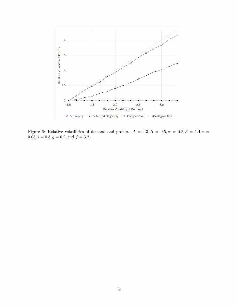
Figure 6: Relative volatilities of demand and profits. A = 4.3, B = 0.5, α = 0.8, β = 1.4, r =0.05, s = 0.3, g = 0.2, and f = 3.2.

58

Figure 7: Relation between the Herfindahl-Hirschman Index and strategic real estate. This figuredepicts the OLS estimation result of a regression equation (26), which corresponds to Prediction 1.White’s heteroskedasticity-consistent standard errors are also reported.

59

(a) 20-quarter rolling volatility

(b) 40-quarter rolling volatility

Figure 8: Relation between the Herfindahl-Hirschman Index and the industry volatility. This figuredepicts the OLS estimation result of a regression equation (27), which corresponds to Prediction 2.White’s heteroskedasticity-consistent standard errors are also reported.

60

(a) 20-quarter rolling volatility

(b) 40-quarter rolling volatility

Figure 9: Relation between strategic capital and the demand uncertainty. This figure depicts theOLS estimation result of a regression equation (29), which corresponds to Prediction 3. The 8-quarter ahead volatility forecast is used. White’s heteroskedasticity-consistent standard errors arealso reported.

61